StarDICE I: sensor calibration bench and absolute photometric calibration of a Sony IMX411 sensor

Abstract

Context. The Hubble diagram of type-Ia supernovae (SNe-Ia) provides cosmological constraints on the nature of dark energy with an accuracy limited by the flux calibration of currently available spectrophotometric standards. This motivates new developments to improve the link between existing astrophysical flux standards and laboratory standards.

Aims. The StarDICE experiment aims at establishing a 5-stage metrology chain from NIST photodiodes to stars, with a targeted accuracy of $1\text{\,}\mathrm{m}\mathrm{m}\mathrm{a}\mathrm{g}$ in $griz$ colors. We present the first two stages, resulting in the calibration transfer from NIST photodiodes to a demonstration $150\text{\,}\mathrm{M}\mathrm{p}\mathrm{i}\mathrm{x}\mathrm{e}\mathrm{l}$ CMOS sensor (Sony IMX411ALR as implemented in the QHY411M camera by QHYCCD). As a side-product, we provide full characterization of this camera which we believe of potential interest in astronomical imaging and photometry and specifically discuss its use in the context of gravitational wave optical follow-up.

Methods. A fully automated spectrophotometric bench is built to perform the calibration transfer. The sensor readout electronics is studied using thousands of flat-field images from which we derive stability, high resolution photon transfer curves and estimates of the individual pixel gain. The sensor quantum efficiency is then measured relative to a NIST-calibrated photodiode, in a well defined monochromatic light-beam from $375$ to $1078\text{\,}\mathrm{nm}$. Last, flat-field scans at 16 different wavelengths are used to build maps of the sensor response, fully characterizing the sensor for absolute photometric measurements.

Results. We demonstrate statistical uncertainty on quantum efficiency below $0.001\text{\,}\mathrm{e}^{-}\mathrm{/}\gamma$ between $387\text{\,}\mathrm{n}\mathrm{m}$ and $950\text{\,}\mathrm{n}\mathrm{m}$, the range being limited by the sensitivity decline of the tested sensor in the infrared. Systematic uncertainties in the bench optics are controlled at the level of $1\text{\times}{10}^{-3}\text{\,}\mathrm{e}^{-}\mathrm{/}\gamma$. Linearity issues are detected at the level of $5\text{\times}{10}^{-3}\text{\,}\mathrm{e}^{-}\mathrm{/}\gamma$ for the tested camera and require further developments to fully correct. Uncertainty in the overall normalization of the QE curve (without relevance for the cosmology, but relevant to evaluate the performance of the camera itself) is 1%. Regarding the camera we demonstrate stability in steady state conditions at the level of $32.5\text{\,}\mathrm{p}\mathrm{p}\mathrm{m}$. Homogeneity in the response is below $1\text{\,}\mathrm{\char 37\relax}$ RMS across the entire sensor area. Quantum efficiency stays above $50\text{\,}\mathrm{\char 37\relax}$ in most of the visible range, peaking well above $80\text{\,}\mathrm{\char 37\relax}$ between $440\text{\,}\mathrm{n}\mathrm{m}$ and $570\text{\,}\mathrm{n}\mathrm{m}$. Differential non-linearities at the level of $1\text{\,}\mathrm{\char 37\relax}$ are detected. A simple 2-parameter model is proposed to mitigate the effect and found to adequately correct the shape of the PTC on half the numerical scale. No significant deviations from integral linearity were detected in our limited test. Static and dynamical correlations between pixels are low, making the device likely suitable for galaxy shape measurements.

1 Introduction

The calibration of wide-field optical surveys is a subject of active research, driven by requirements from the use of type Ia supernovae to measure the evolution of luminosity distance with redshift (the Hubble diagram), one of the main probes of dark energy. Essentially, this measurement involves the comparison of the apparent fluxes of supernovae at different redshifts. Errors in the differential flux calibration between the bluer photometric bands, in which the low redshift events are observed, and the redder bands, in which high redshift events fall, translate directly into a systematic error in the Hubble diagram. In recent studies, the contribution of the calibration uncertainty to the total uncertainty on the dark energy equation of state parameter has been brought down to a level comparable to the statistical uncertainty (Betoule et al., 2014; Scolnic et al., 2018; Jones et al., 2019). The next generation of instruments, in particular the Vera C Rubin observatory, requires a substantial step-forward in terms of photometric accuracy to benefit from the one-order-of-magnitude increase in the available statistics.

StarDICE is one of the experiments aiming at establishing a metrology chain between laboratory flux references (silicon photodiodes calibrated by NIST) and stars from the CALSPEC library of spectrophotometric standards (Bohlin et al., 2020). As supernova surveys are calibrated relative to these standard stars, establishing this chain with sufficient accuracy essentially solves the calibration issue of the Hubble diagram.

With dark currents of the order of $100\text{\,}\mathrm{fA}$ however, the reference photodiodes cannot be used reliably to measure irradiances fainter than $1\text{\times}{10}^{-11}\text{\,}\mathrm{W}\mathrm{/}\mathrm{c}\mathrm{m}\mathrm{{}^{2}}$ and intermediate steps are required to bridge the remaining gap leading to the irradiance of mag 13 stars of the order of $1\text{\times}{10}^{-19}\text{\,}\mathrm{W}\mathrm{/}\mathrm{n}\mathrm{m}\mathrm{/}\mathrm{c}\mathrm{m}\mathrm{{}^{2}}$. Experiments vary in the way they achieve and control the flux reduction between the calibration reference and the target instrument. Examples of proposed strategies are diffusion on a screen (Stubbs et al., 2007, 2010; Tonry et al., 2012; Marshall et al., 2013; Ferguson et al., 2020), and diffusion in a sphere of short light pulses (Coughlin et al., 2018). The most advanced experiment to date (Lombardo et al., 2017; Küsters, 2019; Küsters et al., 2020) uses a combination of diffusion in integrating spheres together with extremely sensitive calibrated photodiodes (Küsters et al., 2022).

The StarDICE proposal consists of a five-stage chain depicted in Fig. 1, which relies on the near-field calibration of an ultra-faint (less than $1\text{\,}\mathrm{\SIUnitSymbolMicro W}$ of optical power) and stable light source which in turn serves as a distant ($\sim 100\text{\,}\mathrm{m}$) in-situ calibration reference for a small astronomical telescope. To achieve this task, sensitive calibrated devices, either cooled CMOS or CCDs, are required to rapidly and accurately map the radiant intensity of this artificial star at short distance ($\sim 20\text{\,}\mathrm{c}\mathrm{m}$). The present paper, the first in a series describing the chain, details the setup of a spectrophotometric test bench built to transfer the NIST photodiode calibration to the nearby calibration sensor with the required $\sim 0.1\text{\,}\mathrm{\char 37\relax}$ accuracy, and demonstrating the first two steps from the chain.

The choice of a suitable sensor deserves some discussion. Since the early 2000s, many applications of image sensors have gradually shifted from charged coupled devices (CCD) to complementary metal oxide semiconductor image sensors (CMOS image sensors or CIS). In the field of astronomy, however, the important characteristics are quantum efficiency (especially in the near infrared), uniformity, and linearity in the response (provided simple corrections such as flat-fielding), and sensitive area. In the case of these characteristics, the field has been well served by the developments in CCD technology such as infrared sensitive ultra-thick substrates, multi-layer coatings, 4-side buttable sensors, and increase in the number of output amplifiers. A recent example is given by the Teledyne e2v CCD250-82 sensor developed for the camera of the Vera Rubin Observatory (Juramy et al., 2014; O’Connor et al., 2016), which combines all these recent developments. As a consequence, professional astronomy experiments still mainly rely on CCDs. Nevertheless, the last decade has seen increased availability of QE-boosting technologies such as backside illumination (BSI) in CIS, improvements in the performance and arrangement of column-parallel ADCs allowing larger area and 3-side buttable sensors. Specific applications are already making use of the advantages of CIS such as the ability to address subsets of individual pixels as in the TAOS-II project (Huang et al., 2021), which uses the Teledyne CIS113 (Wang et al., 2020) with deported ADCs. Another useful characteristic of CIS is the achievement of high frame rates coupled with low readout noise ($\lesssim$$1\text{\,}\mathrm{e}^{-}$), thanks to highly parallel readout. This feature has important potential applications in high-resolution ground-based astronomy which requires short exposure times ($\sim 10\text{\,}\mathrm{ms}$) to freeze the speckle pattern caused by atmospheric turbulence.

In this first study we characterize a camera equipped with the recently available $150\text{\,}\mathrm{M}\mathrm{p}\mathrm{i}\mathrm{x}\mathrm{e}\mathrm{l}$ IMX411ALR Sony CMOS sensor as implemented in the QHY411M camera. With a large $53\text{\times}40\text{\,}\mathrm{mm}$ sensitive area, low dark current without the need of extensive cooling and negligible read-out noise, this sensor appears very convenient for the direct mapping of low irradiance we are pursuing.

The interest in this camera also extends well beyond the StarDICE experiment. The sampling of the large area by small $3.76\text{\,}\mathrm{\SIUnitSymbolMicro m}$ side pixels makes the sensor well suited for wide-field 1m-class telescopes. This kind of instrument is particularly useful in the follow-up of gravitational waves and neutrino events or as survey instrument for the serendipitous discovery of optical transients such as supernovae or kilonovae. This field of research requires a monitoring of multiple sources, rapidly fading and poorly localized ($>1\text{\,}\deg\mathrm{{}^{2}}$ Abbott et al. 2018). The Global Rapid Advanced Network Devoted to Multi-messenger Addicts (GRANDMA, Antier et al. 2020; Aivazyan et al. 2022) needs telescopes with photometric performance similar to the Zwicky Transient Facility (Bellm et al., 2018) (which has a magnitude limit of 21 for $30\text{\,}\mathrm{s}$ exposures in $r$ band) at a significantly lower cost to be replicated at different sites. It is particularly interesting to obtain high efficiency in the near infrared band since it allows the imaging of the peak of the red kilonova component even if the blue is too weak to be detected by 1m-class telescopes and alert the sensitive spectrographs (Metzger, 2019; Andreoni et al., 2019; Abbott et al., 2017). The unknown feature here is the absolute quantum efficiency of the camera over the required wavelength range. A secondary aim of the paper is therefore to study the camera and measure its quantum efficiency as a reference for the GRANDMA collaboration or other potential applications in astronomy.

The rest of the paper is organised as follows. Section 2 provides a detailed description of the instrumental setup. Section 3 gives an overview of the measurement campaign and describes in detail the measurement process. The main results and associated uncertainties are discussed in Section 4. The results are summarized and discussed in section 5.

Figure 1: Metrology chain of the StarDICE experiment, with light detectors in the left column and light sources in the right column. Each arrow represents a step in the chain and the label gives the order of magnitude of the beam intensity, irradiance or spectral irradiance depending if the beam is contained or extended and monochromatic or not. The steps in gray are conducted at NIST (Houston, 2008) and result in a silicon photodiode calibrated against an electrical substitution cryogenic radiometer. The two steps in red are covered in this paper and provide calibrated sensors with a much lower dark current than the photodiode. The rest of the chain leading to astrophysical standards will be the subject of forthcoming papers.

2 Description of the sensor calibration bench

The StarDICE sensor calibration bench is designed to calibrate CCD or CMOS cameras relative to a flux standard established by NIST(Houston, 2008). The light illumination system has been designed to provide both flat-fielding and mono-chromatic local illumination capabilities in order to fully map the camera quantum efficiency and readout gain.

The camera tested in this study is a QHY411M equipped with a back-illuminated monochrome CMOS sensor IMX411ALR. The sensor illuminated area consists of $10\,654\text{\times}14\,206\text{\,}\mathrm{p}\mathrm{i}\mathrm{x}\mathrm{e}\mathrm{l}\mathrm{s}$ ($151.3\text{\,}\mathrm{M}\mathrm{p}\mathrm{i}\mathrm{x}\mathrm{e}\mathrm{l}\mathrm{s}$) with a pixel width of $3.76\text{\,}\mathrm{\SIUnitSymbolMicro m}$ and a saturation capacity around $80\text{\,}\mathrm{k}\mathrm{e}^{-}$. The sensor has a rolling electronic shutter and its ADC array allows 16 bit readout of the pixel array at a maximum frame rate of $2\text{\,}\mathrm{i}\mathrm{m}\mathrm{a}\mathrm{g}\mathrm{e}\mathrm{/}\mathrm{s}$, with adjustable gain. The camera thermoelectrically cools the sensor down to $-45\text{\,}\mathrm{\SIUnitSymbolCelsius}$ (adjustable) and the generated heat is extracted by a closed-loop circulation of water at $16\text{\,}\mathrm{\SIUnitSymbolCelsius}$. The QHY411 camera is connected to the control computer through a USB3 interface, and commands are sent through a python wrapper on top of the QHY SDK. The data were acquired in exposure mode, not in video mode, which we did not manage to get working with from Linux. The tunable electronic bias and amplifier gain of the camera were kept fixed to their respective values of $100$ and $60$, which delivered a gain on the order of $1.2\text{\,}\mathrm{e}^{-}\mathrm{/}\mathrm{A}\mathrm{D}\mathrm{U}$, effectively mapping the sensor dynamics over the 16 bits.

The test camera is mounted on a two-axis linear stage in an optical test bench where it can intercept either a wavelength tunable f/10 monochromatic light beam or a flat-field illumination beam. Other light sensors, in particular a NIST calibrated Hamamatsu S2281 photodiode, are mounted in the same plane and can in turn intercept the same beams. A sketch description of the setup is given in Figure 2.

Intercalibration between detectors is obtained by taking the ratio of their response to illumination by the same monochromatic light-beam. Measurements of the detector uniformity and photon transfer curves (PTC) are obtained from flat-field exposures in the second beam.

Figure 2: Sketch of the optics of the StarDICE sensor calibration bench. The characteristics of the optical elements are given in Table 1. The light provided by the integrating sphere IS1 is filtered by the SP-DK240 monochromator and focused in a plane where the reference (S2281) and target (IMX411) sensors can be positioned thanks to a motorized XY-stage. An aperture stop (Baffle) is used to clean the focused beam from stray light. The half-reflecting plate redirects half of the light beam on a time-stability monitoring camera (IMX174). The linear stage can alternatively bring the sensors in direct view of the second sphere (IS2) providing flat-field illumination.

2.1 Monochromatic beam

The monochromatic light beam is obtained by imaging the horizontal output slit of an integrating sphere (IS1) on the vertical entrance slit of a Czerny-Turner monochromator (SP-DK240) using a relay of two 90° off-axis parabolic mirrors (M1 and M2). The output slit of the monochromator is then imaged on an aperture stop in front of the detector plane by a second relay (M3 and M4). The focal length of the monochromator is $240\text{\,}\mathrm{mm}$ and its turret hosts three $68\text{\times}68\text{\,}\mathrm{mm}$ gratings, accepting input beams with a recommended minimal f-number of 3.9. The diameter and focal length of the off-axis parabolic mirrors (OAP) are given in Table 1. The first relay shapes an $f/4$ input beam which is then extended to $f/12$ by the second relay. The use of mirrors makes the position of the focus point and image shape conveniently achromatic.

Table 1: Diameter and focal length of the OAP mirrors.

Element	diameter	focal length
	[mm (in)]	[mm (in)]
M1	$12.7(1/2)$	$25.4(1)$
M2	$25.4(1)$	$50.8(2)$
M3	$25.4(1)$	$25.4(1)$
M4	$50.8(2)$	$76.2(3)$

Illumination in IS1 is provided by an electronic board in the $3\text{\,}\mathrm{i}\mathrm{n}\mathrm{c}\mathrm{h}$ port featuring 48 LEDs at different central wavelengths. The flux level of each LED is tunable by software. Typically only one is shining at any given time to minimize pollution of the output beam by out-of-band light. A switchable Ar-Hg arc lamp (not shown in Fig. 2) is fitted to the remaining port of the sphere, and is used to determine the wavelength calibration and resolution of the monochromator.

Our target wavelength resolution is of the order of $2\text{\,}\mathrm{nm}$, with gratings of $1200\text{\,}\mathrm{g}\mathrm{/}\mathrm{m}\mathrm{m}$ and a Ebert angle of $18.7\text{\,}\mathrm{\SIUnitSymbolDegree}$. The theoretical dispersion relation therefore varies between $2.92\text{\,}\mathrm{n}\mathrm{m}\mathrm{/}\mathrm{m}\mathrm{m}$ and $3.47\text{\,}\mathrm{n}\mathrm{m}\mathrm{/}\mathrm{m}\mathrm{m}$ over the wavelength range $1100$–$300\text{\,}\mathrm{nm}$. A slit width of $635\text{\,}\mathrm{\SIUnitSymbolMicro m}$ delivers a full width at half maximum (FWHM) ranging between $1.86\text{\,}\mathrm{n}\mathrm{m}$ and $2.2\text{\,}\mathrm{n}\mathrm{m}$. We keep both slits at this fixed width across the entire range to avoid changing the image position and the wavelength calibration. The vertical extent of the image is set by the opening of IS1 output slits which is set around $500\text{\,}\mathrm{\SIUnitSymbolMicro m}$. In this setting, the spatial extent of the image is about $2\text{\times}3\text{\,}\mathrm{mm}$ in the sensor plane. Due to the relatively low wavelength resolution it is necessary to build a full forward model of the measured spectrum of the Hg-Ar calibration arc lamp to derive accurate wavelength calibration from unresolved doublets or triplets of the lamp. The observed spectrum is modeled as a series of lines of adjustable amplitude convolved with a triangular wavelength response whose width is allowed to vary linearly with wavelength. The wavelength calibration is adjusted as a second order polynomial of the wavelength. The background light is developed on a 13-knots B-spline. The model provides a fairly good description of the spectral lamp data as illustrated in Fig. 3 for the two gratings in use. The wavelength correction curves shown in the third row of the figure are applied to all subsequent measurements and bring the uncertainty on the wavelength calibration well below $1\text{\,}\mathrm{nm}$.

Figure 3: Wavelength calibration model for the monochromatic calibration beam. Results for the blue-optimized grating in use for wavelength shorter than $650\text{\,}\mathrm{nm}$ are presented in the left column, results for the infrared-optimized grating are presented in the right column. Top row: Observed spectrum of the Hg-Ar arc lamp (black dots) and best-fit model (red curve). Second row: Difference in the observed spectrum and the best-fit model. Third row: Wavelength calibration component of the best fit model, that is the quantity to be added to the monochromator set wavelength ($\lambda^{M}$) to match the theoretical wavelength of the observed lines ($\lambda$). Last row: Residuals to the wavelength calibration, that is difference in measured and theoretical line wavelength in the air remaining after wavelength calibration for the brightest lines in the lamp spectrum. The RMS in the difference is respectively $0.17\text{\,}\mathrm{n}\mathrm{m}$ and $0.16\text{\,}\mathrm{n}\mathrm{m}$ for the blue and red gratings.

The 50%-reflective beam splitter inserted after the last mirror redirects a fraction of the flux on a CMOS IMX174LLJ sensor which monitors the time stability of the illumination for a given wavelength.

To further clean the main beam from stray light and make the image extension on the detector perfectly stable, the light is focused on a fixed aperture stop slightly smaller than the image, behind which the slowly diverging beam reaches the detectors.

Finally, a shutter at the entrance of the monochromator is used to shut the beam off during measurements of the ambient and stray light level.

2.2 Flat-field illumination beam

The flat-field light beam is provided by a second integrating sphere (IS2) whose 1” output port shines directly on the detectors. The light is provided by 16 LEDs in a $2\text{\,}\mathrm{i}\mathrm{n}\mathrm{c}\mathrm{h}\mathrm{e}\mathrm{s}$ port without wavelength filtering, so that the spectrum of the light emitted out of the sphere corresponds roughly to the narrow spectrum of the shining LED. A measurement of the output spectrum for each of the 16 independent channels is given in Figure 4. The central wavelength ($\bar{\lambda}$) and spectral width (FWHM), together with the wavelength of the flux maxima ($\lambda_{peak}$) in all channels are provided in Table 2.

The intensity of the current flowing in each LED can be tuned independently by software. The integrated surface brightness in the sphere is monitored by a photodiode inserted in the last $1\text{\,}\mathrm{i}\mathrm{n}\mathrm{c}\mathrm{h}$ port of the sphere. Over the full extent of the large IMX411 sensor, the illumination varies by $2.4\text{\,}\%$ peak to valley, according to the mapping of the beam reconstructed from the images taken during the uniformity scan (see Sect. 4.4).

Figure 4: Normalized spectra of the 16 channels of the flat-field light source on a log scale. The UV LED displays some amount of fluorescence light, otherwise the wavelength range of each channel is quite narrow with respect to the typical width of broadband filters.

Table 2: Central wavelength and spectral width in the flat-field light source.

Channel	$\lambda_{peak}$	$\bar{\lambda}$	FWHM
	[nm]	[nm]	[nm]
0	370	381.4	8
1	390	392.4	10
2	418	421.3	11
3	470	473.2	19
4	505	509.8	25
5	521	526.7	30
6	593	591.2	15
7	656	653.6	19
8	688	686.2	19
9	720	716.9	23
10	763	759.9	24
11	811	804.6	27
12	852	843.4	28
13	915	915.3	52
14	942	952.2	42
15	958	956.3	16

3 Dataset

Throughout this study we performed 5 different kinds of measurements:

1. Dark current and readout noise measurements: the sensor is protected from any illumination by an aluminum front cover.

2. Stability measurements: the camera is kept fixed in front of the flat-field beam, at fixed illumination level and fixed exposure time. This experiment is conducted at 4 different (stabilized) temperatures to study temperature dependence.

3. Photon transfer curve and linearity measurements: Same configuration as dataset 2 except that the illumination level is varied by changing either the source brightness or the exposure time. The sensor temperature is kept fixed at $0\text{\,}\mathrm{\SIUnitSymbolCelsius}$ for this measurement and all the remaining ones.

4. Uniformity measurements: hardware configuration similar to dataset 2 except that the position of the sensor is varied, scanning the flat-field beam.

5. Quantum efficiency measurements: interleaved measurements of the brightness of the monochromatic beam with the camera and the reference photodiode. The measurement is repeated scanning every nanometer in wavelength.

We details the specifics of each measurement in the following, except for the dark current measurement which is straightforward.

3.1 Stability measurements

A Large series of images were obtained with the camera roughly aligned on the center of the flat-field beam to test the readout electronics. The fluctuation of the illumination during a sequence at a given flux level can be estimated from measurements with the monitoring photodiode installed in IS2. The fluctuations in the illumination typically drop below $10^{-4}$ RMS, after a warm-up period of $1000\text{\,}\mathrm{s}$ as is shown in Fig. 5.

Figure 5: Top: Evolution of the photocurrent delivered by the monitoring photodiode in the flat-field light source (IS2) with respect to its average over the entire period. Bottom: Relative RMS of the photocurrent computed over 500 successive samples.

The stability measurement is performed around $510\text{\,}\mathrm{nm}$ using LED channel 4. A stabilized current of $10\text{\,}\mathrm{mA}$ is established in the LED and the thermoelectric cooling system of the sensor is set to a target temperature. This was repeated at 4 set points between $-5$ and $10\text{\,}\mathrm{\SIUnitSymbolCelsius}$. The exposure time is set to $500\text{\,}\mathrm{ms}$ which results in an average pixel charge of $36\text{\,}\mathrm{k}\mathrm{e}^{-}$. A first batch of $I=100$ exposures are taken to wait for the cooling and stabilization of the system temperature. The stability measurement is performed on a subsequent batch of $I=100$ exposures. Denoting $q_{p,i}$ the count measured in pixel $p$ in image number $i$, all images containing the same number of pixels $P$, the following statistics can be gathered on the fly for each batch of images:

$$M_{p} = \frac{1}{I}\sum_{i}q_{p,i}$$ (1)

$$V_{p}^{\delta} = \frac{1}{I}\sum_{i}q_{p,i}q_{p+\delta,i}$$ (2)

$$m_{i} = \frac{1}{P}\sum_{p}q_{p,i}$$ (3)

As described in appendix A, the readout gain can be reconstructed from the relation between the temporal mean of individual pixels $M_{p}$ and the mean of the squares $V_{p}^{0}$, while the mean of individual images $m_{i}$ tracks fluctuations in the illumination level.

The individual images are not stored in this approach. Although the absence of storage prevents the use of robust statistics, it is preferred in this study due to the very large size of individual images. Inter pixel products ($V_{p}^{\delta}$ for $\delta>0$) can be stored to study inter-pixel covariances. This is however not needed for the stability study. We keep track of the cooling power of the sensor at the end of image $i$ and $I_{phd}(t)$ the photocurrent delivered by the photodiode during the sequence.

3.2 Photon Transfer Curve and linearity measurements

The measurement of the PTC is similar to that of the stability except that the sensor temperature is now kept fixed at $0\text{\,}\mathrm{\SIUnitSymbolCelsius}$, and the exposure time and LED current are varied. Below, we combine data from 6 different sets whose characteristics are given in Table 3. Sets 1–3 are dedicated to a fine measurement of the gain and linearity on the first third of the scale $<15\text{\,}\mathrm{k}\mathrm{e}^{-}$ which covers the entire dynamic range of the QE measurement. To mitigate potential deviations from Poissonian statistics due to the brighter-fatter effect (see below), the statistics $M_{p}$ and $V_{p}$ are computed on binned pixels, and divided by the number of pixels in the bins to lie on the same ADU scale as the non-binned statistics. Sets 4–6 sample the full scale without binning.

Outside of the sensor calibration bench, we also gathered two supplemental datasets using a simpler illumination source to enable experimental study of correlations between neighboring pixels as a signature for inter-pixel capacitance or brighter-fatter effects (dataset A), and mapping of the individual pixel gain using a large number of images (dataset B and C). In this configuration, the camera was capped with a 3D-printed hollow cone holding a simple $450\text{\,}\mathrm{nm}$ LED behind a diffusive screen. Switching to an external illumination source allowed to free the bench for the calibration of another camera during these time-consuming measurements. The illumination stability with this alternate source is however one order of magnitude worse than what is achieved on the bench. Therefore we do not rely on these supplemental datasets for our baseline determination of the gain. For study A, in addition to the statistics presented in the previous section, we also gather $V_{p}^{01}$ and $V_{p}^{10}$, the mean of the cross-products between immediately neighboring pixels along a line and along a column.

Table 3: Parameter range for the photon transfer curve and linearity datasets

Set	$I$	$\tau_{exp}$	$I_{led}$	Binning	Statistics
		[s]	[mA]
1	10	0.3	10.0 – 49.8	$6\times 6$	$V^{0}$
2	100	0.01 – 1.0	0.0 – 20.0	$6\times 6$	$V^{0}$
3	10	0.01 – 0.3	0.0 – 49.0	$6\times 6$	$V^{0}$
4	100	0.01 – 1.0	0.0 – 40.0	$1\times 1$	$V^{0}$
5	100	0.01 – 3.0	50.0	$1\times 1$	$V^{0}$
6	100	0.01 – 1.0	50.0	$1\times 1$	$V^{0}$
A	300	10	0, 4	$1\times 1$	$V^{0}V^{01}V^{10}$
B	$3000$	10	0, 1, 2, 3, 4	$1\times 1$	$V^{0}$
C	$3000$	10	0, 1, 2, 3, 4	$1\times 1$	$V^{0}$

3.3 Uniformity measurements

The measurement of the uniformity of the camera response is similar to that of the stability, but the camera is moved through 25 positions in a $5\times 5$ grid spanning a square of 60mm side with 15mm resolution in the flat-field beam. The goal is to disentangle variations in the camera response from spatial variations of the illumination. The measurement is only carried at a sensor temperature of $0\text{\,}\mathrm{\SIUnitSymbolCelsius}$ but is repeated for the sixteen LEDs to look for wavelength dependencies. All LEDs are operated at a stabilized current of $10\text{\,}\mathrm{m}\mathrm{A}$ where they deliver of the order of $60\text{\,}\mathrm{k}\mathrm{e}^{-}\mathrm{/}\mathrm{s}$ in a single camera pixel. The exposure time is set to $0.3\text{\,}\mathrm{s}$ so that none of the pixels saturate.

3.4 Quantum efficiency measurements

The quantum efficiency measurement is performed in the range $375$–$1078\text{\,}\mathrm{nm}$, turning on each of the 26 relevant LEDs, one at a time. After turning on one LED, the camera is set to intercept the monochromatic beam, and the corresponding wavelength range is scanned with a $1\text{\,}\mathrm{nm}$ step size. For each wavelength, two successive camera exposures are taken, one with the beam shutter (S) closed and a second with the beam shutter opened. Simultaneously the same exposures are obtained on the monitoring sensor. Once the wavelength range is exhausted, the reference photodiode is brought to intercept the monochromatic beam, and a similar scan is performed using the monitoring sensor and the photodiode. The quantum efficiency estimate is built from these 4 measurements as:

$$QE(\lambda)=\frac{\Phi G}{\tau_{exp}}\frac{e\epsilon_{NIST}(\lambda)}{I_{NIST}}\frac{M_{N}}{M_{C}}$$ (4)

where $\Phi$ is the measured ADU count in the camera, $G$ is the camera gain estimate in $\mathrm{e}^{-}\mathrm{/}\mathrm{A}\mathrm{D}\mathrm{U}$, $\tau_{exp}$ is the exposure time in seconds, $\epsilon_{NIST}$ is the quantum efficiency of the reference sensor in $\mathrm{e}^{-}\mathrm{/}\gamma$, $I_{NIST}$ is the photocurrent delivered by the reference sensor in ampere, $e$ is the elementary charge in coulomb, and $\frac{M_{N}}{M_{C}}$ is the ratio of the count rate in the monitoring sensor during the reference photodiode and camera exposures. We further detail the computation of the different terms in what follows.

3.4.1 Photodiode operations

Our reference sensor is a Hamamatsu S2281 photodiode, with a circular photosensitive area of $1\text{\,}{\mathrm{cm}}^{2}$ ($5.65\text{\,}\mathrm{mm}$ radius). The measurement of its quantum efficiency curve $\epsilon_{NIST}(\lambda)$ performed at NIST (Houston, 2008) along with associated uncertainties is recalled in Figure 6.

Originally built with a non-cooled camera in mind the heat generated by the focal plane cooling slightly exceeded the heat dissipation capability of the sensor calibration bench enclosure resulting in a nominal operation temperature in the range $26.4\text{\,}\mathrm{\SIUnitSymbolCelsius}26.6\text{\,}\mathrm{\SIUnitSymbolCelsius}$. This temperature is slightly larger than the target $23\text{\,}\mathrm{\SIUnitSymbolCelsius}$ temperature at which the reference NIST sensor was calibrated. This introduces a systematic uncertainty in the infrared region due to the change of the photodiode quantum efficiency with temperature. According to Houston (2008, Fig 9.1) the change is only important beyond $1000\text{\,}\mathrm{nm}$ where it amounts to $0.2\text{\,}\%\mathrm{/}\mathrm{\SIUnitSymbolCelsius}$.

Centering of the photodiode in the monochromatic light beam is performed by scanning in x and y at constant illumination past the edges of the photodiode sensitive area. The photodiode is then moved back to the barycenter of the resulting flux map.

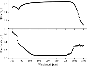
Figure 6: Top: Quantum efficiency curve of our reference Hamamatsu S2281 photodiode as measured by the NIST. Bottom: Quoted relative uncertainty on the quantum uncertainty at the $95\text{\,}\mathrm{\char 37\relax}$ level ($2\sigma$).

The flux level of the monochromatic beam was designed to be relatively low in order to avoid saturation of CCD cameras in relatively long exposures (larger than $1\text{\,}\mathrm{s}$), allowing its use to calibrate cameras with mechanical shutters while minimizing exposure time uncertainties. As a consequence, sensitive readings of the photocurrent required us to select a large feedback resistance in the transimpedance amplifier and limited bandwidth. The photocurrent out of the photodiode is sampled at $7.8\text{\,}\mathrm{Hz}$ by a Keithley 6514 picoammeter. At any given wavelength the photocurrent is sampled for $30\text{\,}\mathrm{s}$, starting $10\text{\,}\mathrm{s}$ before the opening of the monochromatic beam shutter. The shutter is left open for $10\text{\,}\mathrm{s}$ and closed again for the end of the operation. The average shape of the photocurrent reading is plotted in Fig. 7. We construct 3 numerical averages $I_{0}$, $I_{1}$ and $I_{2}$ of the readings before, during and after the light exposure, avoiding the transition regions. We construct the photocurrent estimate as $I_{NIST}=I_{1}-(I_{0}+I_{2})/2$, and estimate uncertainties on $I_{NIST}$ from the standard deviation of the samples in each of the quantities as: $\sigma_{I_{NIST}}^{2}=\sigma_{I_{1}}^{2}+\frac{\sigma_{I_{0}}^{2}+\sigma_{I_{2}}^{2}}{4}$.

Figure 7: Average shape of the photocurrent reading in the NIST-calibrated sensor. The shaded regions corresponds to readings selected to build the photocurrent estimate.

3.4.2 Camera operations during quantum efficiency measurements

We apply the same settings for the quantum efficiency measurement as for the PTC measurement, so that we can assume the readout gain to be identical. In normal mode, we select $2s$ exposures for both the “dark” and “open” exposures.

The estimate of the camera count $\Phi$ at each wavelength is built in several steps. First we compute the centroid of the slit image in the camera by building a stack of all images from a complete wavelength scan. The stack is built as the sum of all open images minus the sum of all dark images. Second, we perform the photometry of all images in circular apertures centered on the computed centroid with physical radii of $2$, $5.65$ and $6\text{\,}\mathrm{mm}$. The second radius matches exactly the physical size of the NIST photodiode, and is very significantly larger than the slit image FWHM of $2.9\text{\,}\mathrm{mm}$. This aperture minimizes systematic errors from small amount of light diffused at large angles (see the discussion in Sect. 4.5). The flux in an aperture of radius $r$ is denoted $\Phi_{r}$. We also gather the sum of all pixels in the image $T$ and compute a background light proxy as $B=T-\Phi_{6}$.

The large apertures, required to match the physical size of the reference sensor, makes the photometry very sensitive to background contamination. We use the “dark” exposures to refine our background estimate as follows. For a given aperture $r$, we adjust a linear relation between $B$ and $\Phi_{r}$ on all the “dark” images in the sequence as $\Phi_{r}=\alpha B+\beta$. An illustration of the fit is given in Fig. 8.

Figure 8: Top: Instrumental flux in $5.65\text{\,}\mathrm{mm}$ apertures measured in “dark” images as a function of the background light proxy build from the never exposed region of the sensor. The best-fit linear relation (solid black line) gives an estimate of background contribution in exposed images. Bottom: Residuals to the best fit relation. The measured rms gives the level of the background subtraction noise which is the dominant noise contribution in our QE measurement.

We then use the best fit parameters to build the background corrected aperture flux as $\bar{\Phi}_{r}=\Phi_{r}-\alpha B-\beta$. Doing so, the uncertainties on background subtraction are typically of the order of $70\text{\,}\mathrm{k}\mathrm{A}\mathrm{D}\mathrm{U}$ for the full $5.65\text{\,}\mathrm{mm}$ aperture and drops down to $15\text{\,}\mathrm{k}\mathrm{A}\mathrm{D}\mathrm{U}$ for the smaller $2\text{\,}\mathrm{mm}$ aperture where it compares more favorably to the photon noise (see the results section for a more detailed discussion of the various noise contributions).

3.4.3 Monitoring sensor

Lastly, we use an IMX174 sensor to monitor changes in illumination while switching between target and reference sensor. When the camera faces the beam, the exposures of the monitoring sensor are synchronized with the camera exposures and the resulting photometry delivers the quantity $M_{c}$ in Eq. (4). With the photodiode in the beam, the monitoring sensor continuously acquires $2\text{\,}\mathrm{s}$ exposures. Images corresponding to opening and closing of the shutter are discarded, and the photometry of the three fully exposed images is averaged to deliver the quantity $M_{N}$ in Eq. (4).

In both case, photometry is performed similar to what was described for the target sensor: we gather photometry in several apertures centered on the centroid of the slit images, and build a background estimator from “dark” images. The only difference is that we are not constrained to match the aperture size of the NIST photodiode for this monitoring measurement, the only important point being that $M_{N}$ and $M_{c}$ are derived from the same aperture so that the ratio of the two corresponds to the variation of the illumination. Therefore we select a much smaller aperture ($1\text{\,}\mathrm{m}\mathrm{m}$) closer to the extent of the image, to optimize the signal to noise ratio.

4 Results

4.1 Sensor cosmetics and inter-pixel capacitance

The sensor cosmetics is studied on a stack of 3000 dark frames with 10s exposures with a stabilized sensor temperature of $0\text{\,}\mathrm{\SIUnitSymbolCelsius}$. The fractions of pixels displaying a level of dark current in excess of $1$, $10$, $100$ and $1000\text{\,}\mathrm{e}^{-}\mathrm{/}\mathrm{s}$ are respectively $5.00\text{\times}{10}^{-4}$, $3.69\text{\times}{10}^{-5}$, $4.11\text{\times}{10}^{-6}$ and $2.08\text{\times}{10}^{-7}$.

We can take advantage of the hot pixels to get a handle on the pattern of the inter-pixel capacitance (IPC, Moore et al. 2004; Finger et al. 2006), which is found to be significant only between two adjacent pixels in a column, with a correlation coefficient of $3.69\pm 0.01\cdot 10^{-3}$. The effect is not symmetric. Pixels with even line numbers are only coupled to the pixel in the following line (respectively odd-parity pixels are coupled to the preceding pixels). The effect on photon statistics is thus half what the correlation constant would suggest. The measured $3\times 3$ correlation pattern between neighboring pixels as seen by pixels with even-parity coordinates is presented in Fig. 9.

Figure 9: Coupling coefficients between neighboring pixels attributed to interpixel capacitance (IPC). The asymmetry of the effect imposes to distinguish between even and odd column and line numbers. In the figure the pattern is presented as it would appear for a central pixel with even line and column coordinates. A pixel with odd line coordinates is instead mostly correlated with the pixel immediately above.

4.2 Stability of the photometric response

The stability of the camera response in time and temperature is obtained from the stability dataset described in Sect. 3.1. A small trend with sensor temperature is detectable in the camera response. Fig. 10 displays the measured response at 4 different stabilized temperatures between $-5$ and $10\text{\,}\mathrm{\SIUnitSymbolCelsius}$. The measurements are well described by a simple linear trend, with a relative slope of $0.027\text{\,}\%\mathrm{/}\mathrm{\SIUnitSymbolCelsius}$. The gain estimate derived from the same dataset is in contrast extremely stable, and compatible with no gain change at the $2\cdot 10^{-4}$ level over the $15\text{\,}\mathrm{\SIUnitSymbolCelsius}$ spanned by the test data. This result suggests that the observed temperature trend is dominated by a change in the sensor quantum efficiency. The test, conceived as a check of the gain stability, was performed at a single wavelength. It would be interesting to repeat the same measurement at different wavelength, especially in the infrared where the strongest temperature dependence is expected.

The result shows that sub-mmag photometric stability is easily achievable even without stringent control of the environment, in particular when operating at a steady framerate. Here, the RMS of the camera average in the second batches of stability exposures (that is, the batch starting after 100 stabilization exposures) is $3.26\text{\times}{10}^{-5}$ on average. This is even lower than the RMS of the monitoring photodiode readings ($\sim 10^{-4}$ see Fig. 5), so that we cannot distinguish between fluctuations in the camera response or in the illumination. The quoted number can be used as an upper bound on the camera response fluctuation in stable conditions.

Figure 10: Relative change in camera response (black circle) and gain (blue squares) with sensor temperature. The black line is a linear fit to the change in camera response.

4.3 Study of the readout electronics

The shape of the relation between the variance and the expectation of the pixel readout across a large range of illumination levels, usually called the photon transfer curve, is a well-documented tool to study the gain of the readout chain of CCD sensors. It was recently extended to the study of the dynamical electrostatic effect, coined as brighter-fatter effect, affecting thick deep-depleted CCD sensors (see Astier et al. 2019 for the modification of the PTC shape and reference therein for a description of the effect).

As a large number of pixels share the exact same readout chain, CCD studies typically rely on statistics built from a large number of pixels and a small number of images. Different levels of spatial averaging are relevant in the study of CIS: averaging over the entire focal plane gives the best handle over features shared by the entire ADC array, such as reference voltages, averaging over individual columns is expected to show defects specific to a single ADC pipeline. Measuring the gain for individual pixels through this technique is however challenging and requires very large statistics. Around $30\,000$ images are required to reach percent accuracy on the individual pixel gain. We present limited but promising efforts in this direction in the next section. As no information is available to us regarding the structure of the sensor readout chain we only assume that it follows a standard column parallel structure.

We propose various models for the statistics $M_{p}$ and $V^{0}_{p}$ and $m_{i}$ in appendix A. In the case where perfect linearity of the pixel response to illumination can be assumed, and where the photo-conversion is a perfect Poisson process (independent conversion events with constant probability), the readout chain is described by 3 parameters: its gain $G$ in $\mathrm{e}^{-}\mathrm{/}\mathrm{A}\mathrm{D}\mathrm{U}$, the readout noise $\sigma$ and the readout bias $b$, which can be inferred from fitting relation (17) to the empirical statistics. Deviations from the linearity or Poissonian hypothesis will appear as deviations from the straight line in the plot. Disentangling between the different effects requires additional data, either direct linearity measurements or extensive study of the correlation between neighboring pixels.

A simple step to mitigate the effect of correlations between neighboring pixels (either from IPC or brighter-fatter) is to compute statistics on pixels made artificially bigger by binning. We first present the study of the average transfer curve of the sensor, obtained by binning pixel counts in $6\times 6$ square superpixels, on the first third of the digital scale which widely encompasses the dynamic range over which the quantum efficiency measurements has been performed. We then present the measurements of the PTC on non-binned statistics over the full-scale as well as direct check of the integral linearity, and nearest neighbors covariances. Those three measurements combined hints toward a consistent picture with good integral linearity and measurable deviation from the Poisson hypothesis. At this stage, however, we cannot provide a complete model satisfactorily describing this dataset. Therefore, we rely on the measurement in binned pixels to infer our baseline value for the camera gain. Finally, we present our measurements of the readout gain uniformity.

4.3.1 Photon transfer curve in $6\times 6$ superpixels

Figure 11: Top: Photon transfer curve for the IMX411 sensor obtained from statistics build from $6\times 6$ binned superpixels over the first third of the scale. The 3 colors corresponds to 3 independent datasets obtained with different illumination, exposure time and number of images (see Table 3). The black solid line presents the linear relation from Eq. (17) using the best fit gain value. Middle: Residuals to the linear model. The dashed black lines figure 1% variations of the integral gain. Bottom: Residuals to the full model, including the effect of a 512-bit periodical DNL with 0.65 ADU of amplitude, and provision for curvature of the PTC due to residual influence of brighter-fatter effect in the binned superpixels.

For each $M_{p}$ and $V_{p}$ in datasets 1–3, we compute the mean variance $V$ of all the $N_{\mu}$ superpixels sharing the same $M_{p}=\mu$ value as follows:

$$V(\mu)=\frac{1}{N_{\mu}}\sum_{\{p,M_{p}=\mu\}}V_{p}-\Delta^{2}(\mu-b)^{2}\,,$$ (5)

where the $\Delta$ term corrects the statistics for the effect of small illumination fluctuations during the measurement (see appendix A.2 for details). This procedure allows us to recover the full resolution of the PTC shape, while a simple averaging over the focal plane would smear the features due to non uniformity in the illumination level. The result is presented in Figure 11. All three datasets are presented on the same plot, and present a rather consistent picture.

The most striking feature is a periodic differential non linearity (DNL) very consistent in all datasets, likely corresponding to a fix bit width error. As striking as it appears on the PTC the DNL likely has little practical consequences. However, it complicates the analysis of the PTC as statistics obtained with slightly different illumination are no longer directly comparable and a simple model for the shape does not describe the data.

When fitting independently a simple linear relation to the three datasets, we recover an average gain value of $1.274\pm 0.0016\text{\,}\mathrm{e}^{-}\mathrm{/}\mathrm{A}\mathrm{D}\mathrm{U}$, where the quoted uncertainty is the RMS between the three datasets. The middle panel in Figure 11 shows the residuals to this simple model for the three datasets. Fitting instead for the approximate shape of the PTC in presence of BF proposed in (Astier et al., 2019, Eq. 16), gives a significantly different average value of $1.2636\pm 0.0023\text{\,}\mathrm{e}^{-}\mathrm{/}\mathrm{A}\mathrm{D}\mathrm{U}$, a $4-\sigma$ difference, with a moderate preference for a non zero curvature of the binned PTC: $a_{00}=-5\pm 2\cdot 10^{-7}$. The recovered values for the curvature are not very consistent between the three datasets, and they change when the top of the scale is cut differently (e.g. at $15\text{\,}\mathrm{k}\mathrm{A}\mathrm{D}\mathrm{U}$) as can be expected from the poor quality of the fit.

A rough model of the DNL can be attempted to improve the fit consistency and enable comparison between statistics at different focal plane locations more easily, alleviating the need for matched illumination levels. In appendix A.3, we present the tools to numerically compute the relevant statistics with arbitrary digital boundaries. We model the DNL as a sine function with a period of 512 bits, that is to say, we assume that the digital scale admits boundaries between codes $D_{n}=n+A_{DNL}\cos\left(\frac{2\pi}{512}(n-\phi_{DNL})\right)$. Not knowing the details of the architecture of the ADC array, little more than that can be done, but this ad-hoc model may be a good-enough description of the reality for the need of the present study. Fitting for $A_{DNL}$ and $\phi_{DNL}$ along with the readout gain and noise delivers a fairly comprehensive description of datasets 1 and 3, although distinctive features remain visible in the residuals as shown in the bottom panel of Fig. 11. The best fit values are $A_{DNL}=0.651\pm 0.006$\mathrm{A}\mathrm{D}\mathrm{U}$$ and $\phi_{DNL}=44.4\pm 0.2$. The corresponding reduced chi-squared for the two datasets are $1.41$ and $1.22$. Interestingly, dataset 2 which is obtained from a much higher number of consecutive frames (see table 3) is at odds with the other two datasets with way less satisfactory fit quality of $\chi^{2}/{d.o.f.}=2.39$. The reasons behind this disagreement are for the moment not understood. However the problem is unlikely to affect the gain determination as all three datasets now deliver a very consistent gain value $G=1.273\pm 0.0008$\mathrm{e}^{-}\mathrm{/}\mathrm{A}\mathrm{D}\mathrm{U}$$, where again the quoted uncertainty is the RMS of the 3 fits. The improved modeling, however, does not entirely solve the inconsistency between the datasets when allowing for curvature. The mean and RMS of the recovered curvature now settles at $a_{00}=-1.6\pm 1.3\cdot 10^{-7}$, compatible with zero and resulting in a slightly lower mean gain value of $G=1.269\pm 0.0035$\mathrm{e}^{-}\mathrm{/}\mathrm{A}\mathrm{D}\mathrm{U}$$. We adopt this last value and its uncertainty as our baseline determination of the readout gain. Due to the binning, this value is not affected by the IPC.

4.3.2 Distinguishing between non linearity and other effects in the full scale PTC

Figure 12: Top: Photon transfer curve for the IMX411 sensor obtained from statistics build from individual physical pixels over the full scale. The 3 colors corresponds to 3 independent datasets obtained with different illumination level and exposure times (see Table 3). The black solid line presents the linear relation from Eq. (17) using the best fit gain value. Middle: Residuals to the linear model. The dashed black lines figure 1% variations of the integral gain. Bottom: Residuals to the full model, including the effect of a 512-bit periodical DNL with 0.65 ADU of amplitude, and provision for curvature of the PTC due to influence of brighter-fatter-like effect in the physical pixels.

The PTC measured directly on individual pixels and over the full scale is presented in Figure 12. The model including both brighter-fatter and 512-bit periodic non-linearity is a rather poor fit of the data, mainly because other differential features show up beyond the 512 bit-periodic feature. The best-fit parameters are however fairly compatible with those previously obtained: $G=$1.273\pm 0.007\text{\,}\mathrm{e}^{-}\mathrm{/}\mathrm{A}\mathrm{D}\mathrm{U}$$, $A_{DNL}=$0.665\pm 0.016\text{\,}\mathrm{A}\mathrm{D}\mathrm{U}$$, and $\phi_{DNL}=49.2\pm 1.7$. The uncertainty on the PTC curvature remains high: $a_{00}=-4.0\pm 1.9\cdot 10^{-7}$, because of the remaining features. We have not attempted to build a comprehensive model of the remaining features at this stage, but reckon that the general shape of the PTC points toward significant non null curvature. Correcting the recovered gain value from the expected influence of the IPC measured on hot pixels (see sect 4.1), brings the gain estimate on the full statistics even closer to the value recovered in binned statistics.

Both classical non linearity and brighter-fatter effect could cause the observed curvature of the PTC. Behavior similar to the brighter-fatter has been previously reported in CMOS (Greffe et al., 2021) and CMOS NIR detectors (Plazas et al., 2018), with a proposed physical mechanism, shrinkage of the depletion region (Plazas et al., 2017), paralleling the mechanism observed in CCDs. Disentangling between classical non linearity or brighter-fatter effect necessitates either direct linearity measurements or detection of the characteristic correlation between neighboring pixels introduced by the electrostatic influence. We present both measurements in Figures 13 and 14.

The dataset specifically taken to study correlations (A in Table 3) provides moderate evidence for the presence of positive correlations between the nearest neighbors in a line ($C_{01}$) and in a column ($C_{10}$), in excess of what would be expected from measured IPC alone. The resulting curves are shown in Figure 13. The shape does not readily comply with expectations for BF-induced correlations and we don’t have at this stage a compelling model for the measured shape. The most obvious caveat in the data-set is the need to subtract for the contribution of quite large illumination fluctuations ($\Delta\sim 10^{-3}$). This is done using the RMS of the mean of all images in the sequence to build an estimate of the illumination fluctuation (see appendix A.2). We note that the proposed technique would allow investigation of the correlations at larger distances $C_{ij}$, however adequate hardware to perform the required comparatively heavy computations in real time would be required.

Figure 13: Measured covariances between the nearest neighbors in a line ($C_{01}$) and in a column ($C_{10}$) as a function of pixel readout. The dashed lines figure the corresponding expected covariances from the measured IPC. The black dashed line figures the first-order shape of the correlation expected for an amplitude of the correlation factor corresponding to $\frac{-a_{00}}{2}$, with $a_{00}$ the best fit value from the PTC.

Figure 14: Direct linearity check performed by interlacing measurements at increasing exposure time and increasing brightness. Dot intensity encodes the exposure time. Top: Average illumination level in the camera as a function of the modeled illumination intensity in the flat-field source. Bottom: Difference between measured camera level and the modeled flat-field source intensity. The dashed black lines figure variation of the integral gain by $\pm 0.1\%$.

The flat-field illumination source was built with the idea of providing a direct linearity measurement, but at this stage the linearity of the illumination has not yet been calibrated. The gathered dataset still allows limited investigation of the linearity by interlacing variations of the illumination (through variation of the LED intensity), with variations of the exposure time, and solving for illumination level at a given LED intensity. Doing so gives the linearity check presented in Fig. 14, which does not detect significant integral non-linearities in the chain up to $55\,000\text{\,}\mathrm{A}\mathrm{D}\mathrm{U}$ ($70\text{\,}\mathrm{k}\mathrm{e}^{-}$).

We therefore conclude that the curvature observed in the PTC is not attributable to classical non-linearity and is at least qualitatively compatible with expectations from a small brighter-fatter effect.

4.3.3 Uniformity of the readout gain

Determination of the individual pixel gains using this technique requires a very large number of images, but is in principle achievable. We made an attempt to test the concept with the high statistics datasets denoted (B) and (C) in Table 3. The result is presented in the left panel in Fig. 15. The main visible feature in the recovered gain map is the imprint of the differential non-linearity due to the smooth change in illumination level in the flat-field images. Simply correcting the measured variance using the ad-hoc model from Fig. 11, gives the per-pixel mean-over-variance map presented on the right-panel. Residual features in the corrected map show that the applied correction is not fully adequate across the focal plane, but at least qualitatively describe the phenomenon. The corrected map has an RMS of $1.7\%$, dominated by statistical noise. Binning the map by $120\times 120$ pixel to suppress the statistical noise brings the RMS down to $1.0\%$, with residual artifacts from the DNL dominating the spatial features. Therefore we conclude that we can set an upper bound of $1\%$RMS on spatial variations of the effective gain value across the focal plane. In addition the average gain in the region illuminated in the quantum efficiency measurement differs from the focal-plane average by $0.0008\text{\,}\mathrm{e}^{-}\mathrm{/}\mathrm{A}\mathrm{D}\mathrm{U}$. Therefore, we stick to the baseline gain value to interpret our quantum efficiency measurement.

Figure 15: Left: Uncorrected map of the individual pixel gain obtained from 12000 images at 4 different illumination levels. The circular features arise from a periodic differential non linearity imprinted on the gain estimate due to a center-to-edge gradient in the illumination pattern. Right: Same as before but correcting the measured empirical variance for the prediction of the non-linearity model adjusted in Fig. 11.

4.4 Uniformity of the camera response

The camera response (i.e. the product of the quantum efficiency and the readout gain) has been mapped at the 16 wavelengths delivered by the flat-field light source. Given that the spatial extent of the IMX411 sensor is larger than the area over which the flat-field beam can be considered uniform, we resorted to iteratively solve for the intensity of the illumination pattern and the camera response map. The 25 images in a single wavelength dataset are thus interpreted as the product of the illumination pattern $B(\@vec{x})$ at this wavelength with the camera response map $M(\@vec{x})$ for 25 known central positions $x_{i}$ of the camera. Image $i$ therefore follows the equation:

$$I_{i}(\@vec{x})=B(\@vec{x}+\@vec{x}_{i})\times M(\@vec{x})\,.$$ (6)

The illumination pattern over the full area is developed on a cardinal bicubic B-spline basis with $10\times 10$ nodes. A first estimate of the illumination pattern $B^{0}$ is obtained assuming a uniform camera response $M^{0}=1$, and this $B^{0}$ is used to solve for a first map of the camera response $M^{1}$. The procedure is iterated once and quickly converges. The model is an accurate description of the dataset except for projective features such as defects on the camera window.

Figure 16: Map of the transmission uniformity for the 16 different flat-field channels, corresponding to different illumination wavelength from UV to near infrared. The scale of the map is relative to the average response over the entire sensor area. The black contour figures the region in which the high-resolution quantum efficiency curve measurement has been performed.

The resulting camera response maps are shown in Figure 16. All demonstrate uniformity in the response at the level of $4\%$ peak-to-peak ($<1\%$ RMS), with the position selected for the QE measurement being in general slightly below the average. The pattern shows some evolution with wavelength, however, the evolution appears slow enough to be corrected by filter-dependent flat-fielding, with an accuracy dependent on the chosen photometric system.

4.5 Quantum efficiency curve

Our quantum efficiency measurement is obtained from Eq. (4) using the baseline gain estimate of $1.269\text{\,}\mathrm{e}^{-}\mathrm{/}\mathrm{A}\mathrm{D}\mathrm{U}$ obtained in Sect. 4.3.1. The measurement was performed three times and then the optical configuration was varied to look for systematic errors. The 3 independent measurements are presented in Fig. 17.

Figure 17: Top: Quantum efficiency curve of the QHY411M camera (window included). Three independent measurements at the same location are superimposed. The solid black line correspond to a smooth B-spline fit to the data. Middle: Residuals to the B-spline fit. The three colors correspond to the three independent measurements. Bottom: Breakout of the noise in the quantum efficiency measurement according to the origin of the contribution from the four different terms in Eq. (4). The plot also presents the quadratic sum of the four contributions (solid black line) and the RMS of the 3 independent measurements recalled from the middle panel (dotted black line).

The largest systematic uncertainties affecting the overall scale of the curve are i) the uncertainties in the gain determination and ii) the $1$% calibration uncertainty of the picoammeter reading the photocurrent of the NIST reference sensor. Those uncertainties affect the overall scale of the curve which therefore peaks at $0.84\pm 0.01\text{\,}\mathrm{e}^{-}\mathrm{/}\mathrm{A}\mathrm{D}\mathrm{U}$ for the measured position. The quantum efficiency stays above $80\%$ in the range $440\text{\,}\mathrm{nm}570\text{\,}\mathrm{nm}$, above $50\%$ in the range $387\text{\,}\mathrm{nm}650\text{\,}\mathrm{nm}$ and above $20\%$ all the way up to $790\text{\,}\mathrm{n}\mathrm{m}$.

The breakout of the noise contribution from the various components in Eq. (4) to the statistical uncertainty is presented in the bottom panel of Figure 17, along with the RMS of 3 measurements. The quadratic sum of the contributions nicely lines up with the observed RMS of the measurements. The uncertainty is dominated by background noise in the IMX411 sensor because a very large aperture, matching exactly the spatial extent of the NIST sensor, is used in order to minimize aperture correction systematics. The statistical uncertainty on a single measurement with nm resolution is smaller than $0.001\text{\,}\mathrm{e}^{-}\mathrm{/}\gamma$ over the majority of the range and smaller $0.01\text{\,}\mathrm{e}^{-}\mathrm{/}\gamma$ everywhere.

Systematic uncertainties associated with the NIST calibration of the reference photodiode are subdominant at this stage. We looked at two other potential sources for systematic chromatic uncertainties. First, a wavelength-dependent error would arise if the sensitive area of the reference sensor and of the photometric aperture in the camera were not perfectly matched, because the position and the shape of the projected slit image changes slightly with wavelength. We tested this possibility by stopping down the physical aperture in front of the sensor by a factor of 2 in radius. This reduces the spatial extent of the illuminated area on the sensor in all directions and makes the measurement less sensitive to alignment issues. The difference between the baseline and the stopped down measurement is presented on the left panel in Fig. 18. It suggests that the aperture mismatch systematics are controlled at the $0.001\text{\,}\mathrm{e}^{-}\mathrm{/}\gamma$ level.

Figure 18: Left: Difference between the baseline and stopped down measurement of the IMX411 quantum efficiency curve. Right: Difference between two quantum efficiency measurements using 4s and 2s exposures.

Finally, we looked at the potential impact of the non linearities on the QE measurement. Non linearities may affect the measurement because the illumination level is not constant across all wavelengths. We tested this by doubling the camera exposure time and redoing the same measurement. The difference between the two measurements is presented on the right panel in Fig. 18. The observed difference reaches $0.005\text{\,}\mathrm{e}^{-}\mathrm{/}\gamma$ peak-to-peak, dominating the chromatic uncertainty budget. In principle the effect of non-linearities could be corrected but this correction was not attempted at this stage. A specific measurement of the sensor integral linearity and exposure time involving a precisely pulsed light source is planned for the upgrade.

5 Conclusion

The StarDICE sensor calibration bench presented above delivers quantum efficiency measurements with statistical uncertainties below ${10}^{-3}\text{\,}\mathrm{e}^{-}\mathrm{/}\gamma$ in the range $387\text{\,}\mathrm{nm}950\text{\,}\mathrm{nm}$ ($<{10}^{-2}\text{\,}\mathrm{e}^{-}\mathrm{/}\gamma$ in the range $375\text{\,}\mathrm{nm}1078\text{\,}\mathrm{nm}$) and low systematic uncertainties ($\sim{10}^{-3}\text{\,}\mathrm{e}^{-}\mathrm{/}\gamma$) in quantum efficiency ratios between different wavelengths, which is the metric relevant for the measurement of type-Ia supernovae colors. The measurement is sensitive to sensor non-linearities due to the change in illumination intensity as a function of wavelength in the monochromatic beam. A dedicated measurement of the sensor linearity is therefore required to reach the requirements of StarDICE and the addition of a tunable pulsed light source to the bench is planned for this purpose. The systematic uncertainty on the gray-scale is currently dominated by the calibration uncertainty of the picoammeter providing the photocurrent of the reference photodiode.

The sensor calibration bench has been used for the calibration of the quantum efficiency of a QHY411M camera hosting the $150\text{\,}\mathrm{M}\mathrm{p}\mathrm{i}\mathrm{x}\mathrm{e}\mathrm{l}\mathrm{s}$ IMX411ALR sensor from Sony. The camera was found to provide excellent response stability ($<0.0033\text{\,}\%$ RMS in stable conditions). Quantum efficiency is above 80% in the range $440\text{\,}\mathrm{nm}570\text{\,}\mathrm{nm}$, above $50\text{\,}\%$ on most of the visible range, above $20\text{\,}\%$ all the way up to $790\text{\,}\mathrm{nm}$ and close to $10\text{\,}\%$ at $900\text{\,}\mathrm{n}\mathrm{m}$. This translates to an average quantum efficiency in each of the photometric bands of the $ugrizy$ system of respectively $47\text{\,}\mathrm{\char 37\relax}$, $79\text{\,}\mathrm{\char 37\relax}$, $59\text{\,}\mathrm{\char 37\relax}$, $27\text{\,}\mathrm{\char 37\relax}$, $10\text{\,}\mathrm{\char 37\relax}$ and $2\text{\,}\mathrm{\char 37\relax}$. The uniformity of the sensor response is at or below the $1\text{\,}\%$ RMS level for all tested wavelengths. The sensor cosmetics is also excellent. Degradation of the images from electrostatic influence between pixels is expected to be negligible for most use cases given the small measured size of the linear IPC and brighter-fatter effect. This is especially appreciable for $3.76\text{\,}\mathrm{\SIUnitSymbolMicro m}$ pixel side. The only adverse effect found at this stage is a rather large periodical differential non-linearity, despite apparently good integral linearity. Such effects, commonly affecting ADCs, can require correction in applications sensitive to differential linearity, typically those measuring fluctuations around a variable level (see e.g. Planck Collaboration et al. 2020 for a successful account of a posteriori corrections for ADC non-linearities in the context of the measurement of CMB fluctuations). A two-parameter periodic alteration of the scale is sufficient to mitigate the effect on the PTC up to $\sim 20\text{\,}\mathrm{k}\mathrm{e}^{-}$. More complex alteration would be required to describe the entire scale, which was not attempted. Also our integral linearity test relies on the accuracy of the rolling shutter timing, which we did not control. We suggest that applications sensitive to linearity may want to envision adequate mapping of the scale.

We conclude that the sensor is very well suited for many astronomical applications in the visible range. For the GRANDMA experiment, this applies to the search of the optical counterparts of transitory events with poor localization from gravitational wave or neutrino detections which can be conducted in band $g$ and $r$. The characterization of transients through their strong color evolution will however require separated follow-up. Given the relatively low QE of the camera ($27\text{\,}\%$) in the $i$ band) longer exposures would be required to reach adequate sensitivity for hunting kilonovae, necessitating trade-off with survey size. Additionally, we note that the relatively high QE in the $u$-band ($47\text{\,}\%$) could be useful to capture the earliest light of kilonovae in a particularly important band for enabling model selection, provided that the source is detected early enough.

The goal of the StarDICE experiment to control calibration systematic uncertainties from $375\text{\,}\mathrm{nm}$ to $1050\text{\,}\mathrm{nm}$ at the $0.1\text{\,}\%$ level appears difficult to reach in this first measurement due to the low quantum efficiency beyond $900\text{\,}\mathrm{nm}$. The StarDICE calibration sensor bench is therefore being upgraded to increase the flux of the input light-source in the infrared and to calibrate a $40\text{\,}\mathrm{\SIUnitSymbolMicro m}$ deep-depleted CCD sensor more sensitive at these wavelengths. Other ongoing improvements include custom dust-protective housing for the reference sensor, heat and temperature management, upgrade of opto-mechanical parts to ease the alignment of the optics, improved calibration of the reference sensor photocurrent reading and dedicated measurement of the sensor linearity.

Acknowledgements

The authors thank the QHY company for providing the camera tested in this study and for kindly answering our questions. Warm thanks are also addressed to Pierre Astier and Pierre Antilogus for thoughtful discussions and comments on DNL issues, and to Parker Fragelius and Elana Urbach for their help in improving the text. This work received support from the Programme National Cosmology et Galaxies (PNCG) of CNRS/INSU with INP and IN2P3, co-funded by CEA and CNES and from the DIM ACAV program of the Île-de-France region.

Appendix A Statistical model of the photon transfer curve

A.1 Simplest model, perfect illumination, perfect linearity

Let’s first consider an oversimplified model, where we assume independence between successive images, a simple model of white Gaussian readout noise, perfect linearity of the readout chain and ignore potential electrodynamics effects such as the so-called brighter-fatter effect strongly affecting the shape of the PTC in thick deep-depleted CCDs.

The ADU counts in pixel $p\in[1,\cdots,P]$ and image $i\in[1,\cdots,I]$ is then:

$$q_{p,i}=\frac{N_{p,i}+n_{p,i}}{G_{p}}+b_{p}$$ (7)

where $N_{p,i}\sim\mathcal{P}(\bar{N}_{p,i})$ is the number of photoelectron converted and stored in pixel $p$ expected to follow a Poisson distribution, $G_{p}$ is the effective gain of the readout for the pixel (in $\mathrm{e}^{-}\mathrm{/}\mathrm{A}\mathrm{D}\mathrm{U}$), $n_{p,i}\sim\mathcal{N}(0,\sigma_{p}^{2})$ is the noise in the readout expressed in $e^{-}$, and $b_{p}$ is the tunable bias of the readout electronic in $\mathrm{A}\mathrm{D}\mathrm{U}$. The statistics defined in equations (1-3) have the following properties:

$$\operatorname{\mathbb{E}}[M_{p}] = \frac{1}{IG_{p}}\sum_{i}\bar{N}_{p,i}+b_{p}$$ (8)

$$\operatorname{var}[M_{p}] = \frac{1}{I^{2}G^{2}_{p}}\sum_{i}\bar{N}_{p,i}+\frac{\sigma_{p}^{2}}{G^{2}I}$$ (9)

$$\operatorname{\mathbb{E}}[M_{p}^{2}] = \operatorname{\mathbb{E}}[M_{p}]^{2}+\operatorname{var}[M_{p}]$$ (10)

$$\operatorname{\mathbb{E}}[V_{p}^{0}] = \frac{1}{I}\sum_{i}\operatorname{var}[q_{p,i}]+\operatorname{\mathbb{E}}[q_{p,i}]^{2}$$ (11)

$$= \frac{\sigma_{p}^{2}}{G_{p}^{2}}+\frac{\sum_{i}\bar{N}_{pi}}{IG_{p}^{2}}+\frac{\sum_{i}\left(\frac{\bar{N}_{p,i}}{G_{p}}+b_{p}\right)^{2}}{I}$$ (12)

Under perfect stability of the illumination conditions, that is $\bar{N}_{p,i}=\bar{N}_{p}$, the above simplify as:

$$\operatorname{\mathbb{E}}[M_{p}] = \frac{\bar{N}_{p}}{G_{p}}+b_{p}$$ (13)

$$\operatorname{var}[M_{p}] = \frac{\bar{N}_{p}}{IG_{p}^{2}}+\frac{\sigma_{p}^{2}}{IG_{p}^{2}}$$ (14)

$$\operatorname{\mathbb{E}}[V_{p}^{0}-M_{p}^{2}] = \frac{\sigma_{p}^{2}}{G_{p}^{2}}+\frac{\bar{N}_{p}}{G_{p}^{2}}$$ (15)

$$\operatorname{\mathbb{E}}[V_{p}^{0}-M_{p}^{2}]=\frac{I-1}{I}\left(\frac{\operatorname{\mathbb{E}}[M_{p}]-b}{G_{p}}+\frac{\sigma_{p}^{2}}{G_{p}^{2}}\right)$$ (17)

In this simple model, the slope of the relation between the two observables $V^{0}_{p}-M_{p}^{2}$ and $M_{p}$ gives a direct estimate of the effective readout gain, while the intercept is a measurement of the read noise.

The uncertainty on the determination of $G$ scales as $2/\sqrt{I}$, which indicates that a determination of $G_{p}$ at $1$% would require of the order of $3\cdot 10^{4}$ images.

A.2 Accommodating illumination variations

The model can easily be extended to accommodate small fluctuations of the illumination. Let us write $\bar{N}_{p,i}=\bar{N}_{p}(1+\Delta_{i})$ where we take by definition $\sum_{i\in I}\Delta_{i}=0$. Denoting $\Delta^{2}=\frac{\sum\Delta_{i}^{2}}{I}$, the expectation of $V^{0}_{p}$ is modified as:

$$\operatorname{\mathbb{E}}[V^{0}_{p}]=\frac{\bar{N}_{p}}{G_{p}^{2}}+\left(\frac{\bar{N}_{p}}{G_{p}}+b_{p}\right)^{2}+\frac{\sigma_{p}^{2}}{G_{p}^{2}}+\Delta^{2}\frac{\bar{N}_{p}^{2}}{G_{p}^{2}}$$ (18)

and therefore the relation becomes:

$$\operatorname{\mathbb{E}}[V_{p}-M_{p}^{2}]=\frac{I-1}{I}\left(\frac{\operatorname{\mathbb{E}}[M_{p}]-b_{p}}{G_{p}}+\frac{\sigma_{p}^{2}}{G_{p}^{2}}\right)+\Delta^{2}(\operatorname{\mathbb{E}}[M_{p}]-b_{p})^{2}$$ (19)

Close to the full-well $(\operatorname{\mathbb{E}}[M_{p}-b_{p}]\sim 5\cdot 10^{5})$, illumination fluctuations of the order of $10^{-4}$ would contribute a bias of the order of $0.5\text{\,}\%$, which may deserve some compensation to investigate non-linearity at this level of accuracy. As fluctuations of this order of magnitude are occasionally observed, we choose to estimate $\Delta$ from the empirical variance of the third observable $m_{i}$. Specifically denoting $m=\frac{1}{N}\sum_{i}m_{i}$, $v=\frac{1}{N}\sum_{i}m_{i}^{2}$, $\bar{N}=\frac{1}{P}\sum\frac{\bar{N}_{p}}{G_{p}}$, $B=\frac{1}{P}\sum b_{p}$, $\sigma^{2}=\frac{1}{P}\sum\frac{\sigma_{p}^{2}}{G_{p}}$, and $G=\frac{\sum\bar{N}_{p}/G_{p}}{\sum\bar{N}_{p}/G_{p}^{2}}$ we have that:

$$\operatorname{\mathbb{E}}[v-m^{2}]=\frac{I-1}{I}\left(\frac{\bar{N}}{PG}+\frac{\sigma^{2}}{P}\right)+\Delta^{2}\bar{N}^{2}$$ (20)

and we form:

$$\hat{\Delta}^{2}=\frac{v-m^{2}-(I-1)\sigma^{2}/(PI)}{(m-B)^{2}}$$ (21)

The estimate $\hat{\Delta}$ is used to subtract the contribution to Eq. (20) from reported statistics.

A.3 Probability mass function of pixels with variable bit size

The most striking feature of the readout chain we tested is a periodical differential non-linearity, well reproducible across the focal plane. Although the details of the readout chain are not known to us, this could be interpreted as inaccurate bit widths affecting, e.g. a shared ramp in a ramp-compare ADC scheme. We suggest to handle such effects by numerical computation of the probability mass function for the pixel value. Let us denote $B$ the resolution of the ADC. We then define for $n\in{1,\cdots,2^{B}-1}$, $D_{n}=\sum_{k=0}^{Nbits-1}(1+\delta_{k})(2^{k}\land n)$ the successive values generated by the ramp DAC, where $\land$ denote the binary and operator, and $\delta_{k}$ is the small error on the size of the $k^{th}$ DAC bit. Furthermore we pose $D_{0}=-\infty$ and $D_{2^{B}}=\infty$. The probability mass function for the value of the pixel $P(p=n)$ (dropping indices for clarity) is 0 for $n<0$ and $n\geq 2^{B}$ and:

$$P(p=n) =P\left(D_{n}\leq\frac{N}{G}+n<D_{n+1}\right)$$ (22)

$$=\sum_{k=0}^{\infty}P(N=k)P\left(D_{n}-\frac{k}{G}<n<D_{n+1}-\frac{k}{G}\right)$$ (23)

$$=\sum_{k=0}^{\infty}\frac{\bar{N}^{k}e^{-\bar{N}}}{k!}\frac{1}{2}\left[\operatorname{erf}\left(\frac{D_{n+1}-\frac{k}{G}-b}{\sqrt{2}\sigma}\right)-\operatorname{erf}\left(\frac{D_{n}-\frac{k}{G}-b}{\sqrt{2}\sigma}\right)\right]$$ (24)

from which we obtain the expectation and variance of the pixel value for a given illumination. In practice, the above can be truncated into the product of finite matrices $P=R(G,b,\sigma,\delta)\otimes Q(\bar{N})$. We apply the truncation $Q_{k}(\bar{N})=\frac{\bar{N}^{k}e^{-\bar{N}}}{k!}$ for $\mathrm{min}(0,\bar{N}-5\sqrt{\bar{N}})\leq k<\bar{N}+5\sqrt{\bar{N}}+4$ and $0$ elsewhere. Similarly zeroing $R_{n,k}$ for $|n-\frac{k}{G}-b|>6\sigma$ adequately speed up the computation. We provide a python code using sparse matrix algebra to compute the probability mass function of the pixels with arbitrary digital boundaries and the observable statistics.

A.4 Brighter-fatter effect

Effects like the brighter-fatter could alter the above statistics. As the probability of having a photon converted in a given pixel depends on the charge already accumulated in the pixel, $q_{p,i}$ is no longer Poisson distributed. A first order model of the pdf can be built assuming that the shrinkage of the pixel area (or for what matters of the depletion region in CIS) is proportional to the fluctuation of the charge above the mean, with proportionality constant $a$.

$$I_{k}(t)=I\left(1+a(\operatorname{\mathbb{E}}[N(t)]-k)\right)$$ (25)

For the integration the effect needs to saturate in some way, as the equation above would lead to non physical values. The saturation of the tested sensor ensure that $k\lessapprox$70\text{\,}\mathrm{k}\mathrm{e}^{-}$$, so that the equation will remain well behaved on the useful range for the anticipated value of the proportionality constant $a\sim 10^{-7}$. Let us denote $P_{k}(t)=P(N(t)=k)$ the probability of counting $k$ electrons in the pixel at time $t$. Counting events obeys the following conditional probabilities:

$$P\left[N(t+h)=k+1|N(t)=k\right] = hI_{k}(t)+o(h)$$ (26)

$$P\left[N(t+h)=k+1|N(t)=k+1\right] = 1-hI_{k+1}(t)+o(h)$$ (27)

from which we deduce the differential equation verified by $P_{k}(t)$:

$$\dot{P}_{0} = -I_{0}P_{0}$$ (28)

$$\dot{P}_{k} = I_{k-1}P_{k-1}-I_{k}P_{k}\quad\forall k,0<k<K$$ (29)

$$\dot{P}_{K} = I_{K-1}P_{K-1}$$ (30)

A numerical integration of the system shows that all this is very well approximated by a Gaussian distribution with appropriate variance given by (Astier et al. 2019, Eq. 16). As a shortcut, the Gaussian approximation with modified variance is used in place of the Poisson distribution to compute matrix $Q$ in equation (22) when brighter-fatter effect is taken into account in the PTC model.

References

- Abbott et al. (2018) Abbott, B. P., Abbott, R., Abbott, T. D., Abernathy, M. R., & others. 2018, Living Reviews in Relativity, 21, 3
- Abbott et al. (2017) Abbott, B. P., Abbott, R., Abbott, T. D., et al. 2017, ApJ, 848, L12
- Aivazyan et al. (2022) Aivazyan, V., Almualla, M., Antier, S., et al. 2022, MNRAS, 515, 6007
- Andreoni et al. (2019) Andreoni, I., Anand, S., Bianco, F. B., et al. 2019, PASP, 131, 068004
- Antier et al. (2020) Antier, S., Agayeva, S., Almualla, M., et al. 2020, MNRAS, 497, 5518
- Astier et al. (2019) Astier, P., Antilogus, P., Juramy, C., et al. 2019, A&A, 629, A36
- Bellm et al. (2018) Bellm, E. C., Kulkarni, S. R., Graham, M. J., et al. 2018, Publications of the Astronomical Society of the Pacific, 131, 018002
- Betoule et al. (2014) Betoule, M., Kessler, R., Guy, J., et al. 2014, A&A, 568, A22
- Bohlin et al. (2020) Bohlin, R. C., Hubeny, I., & Rauch, T. 2020, AJ, 160, 21
- Coughlin et al. (2018) Coughlin, M. W., Deustua, S., Guyonnet, A., et al. 2018, in Society of Photo-Optical Instrumentation Engineers (SPIE) Conference Series, Vol. 10704, Observatory Operations: Strategies, Processes, and Systems VII, 1070420
- Ferguson et al. (2020) Ferguson, P. S., Barba, L., DePoy, D. L., et al. 2020, in Society of Photo-Optical Instrumentation Engineers (SPIE) Conference Series, Vol. 11447, Society of Photo-Optical Instrumentation Engineers (SPIE) Conference Series, 114475U
- Finger et al. (2006) Finger, G., Beletic, J. W., Dorn, R., et al. 2006, in Astrophysics and Space Science Library, Vol. 336, Astrophysics and Space Science Library, ed. J. E. Beletic, J. W. Beletic, & P. Amico, 477
- Greffe et al. (2021) Greffe, T., Smith, R., Sherman, M., et al. 2021, arXiv e-prints, arXiv:2112.01691
- Houston (2008) Houston, J. M. 2008, NIST Special Publication, 250, 41
- Huang et al. (2021) Huang, C.-K., Lehner, M. J., Granados Contreras, A. P., et al. 2021, PASP, 133, 034503
- Jones et al. (2019) Jones, D. O., Scolnic, D. M., Foley, R. J., et al. 2019, ApJ, 881, 19
- Juramy et al. (2014) Juramy, C., Antilogus, P., Bailly, P., et al. 2014, in Society of Photo-Optical Instrumentation Engineers (SPIE) Conference Series, Vol. 9154, High Energy, Optical, and Infrared Detectors for Astronomy VI, ed. A. D. Holland & J. Beletic, 91541P
- Küsters et al. (2020) Küsters, D., Bastian-Querner, B., Aldering, G., et al. 2020, in Society of Photo-Optical Instrumentation Engineers (SPIE) Conference Series, Vol. 11447, Society of Photo-Optical Instrumentation Engineers (SPIE) Conference Series, 1144771
- Küsters et al. (2022) Küsters, D., Bastian-Querner, B., Aldering, G., et al. 2022, in Ground-based and Airborne Instrumentation for Astronomy IX, ed. C. J. Evans, J. J. Bryant, & K. Motohara, Vol. 12184, International Society for Optics and Photonics (SPIE), 121847V
- Küsters (2019) Küsters, D. 2019, PhD thesis, Humboldt-Universität zu Berlin, Mathematisch-Naturwissenschaftliche Fakultät
- Lombardo et al. (2017) Lombardo, S., Küsters, D., Kowalski, M., et al. 2017, A&A, 607, A113
- Marshall et al. (2013) Marshall, J. L., Rheault, J.-P., DePoy, D. L., et al. 2013, arXiv e-prints, arXiv:1302.5720
- Metzger (2019) Metzger, B. D. 2019, Living Reviews in Relativity, 23, 1
- Moore et al. (2004) Moore, A. C., Ninkov, Z., & Forrest, W. J. 2004, in Society of Photo-Optical Instrumentation Engineers (SPIE) Conference Series, Vol. 5167, Focal Plane Arrays for Space Telescopes, ed. T. J. Grycewicz & C. R. McCreight, 204–215
- O’Connor et al. (2016) O’Connor, P., Antilogus, P., Doherty, P., et al. 2016, in Society of Photo-Optical Instrumentation Engineers (SPIE) Conference Series, Vol. 9915, High Energy, Optical, and Infrared Detectors for Astronomy VII, ed. A. D. Holland & J. Beletic, 99150X
- Pace (2021) Pace, F. 2021, PhD thesis, thèse de doctorat dirigée par Magnan, Pierre Photonique et Systèmes Optoélectronique Toulouse, ISAE 2021
- Planck Collaboration et al. (2020) Planck Collaboration, Akrami, Y., Argüeso, F., et al. 2020, A&A, 641, A2
- Plazas et al. (2018) Plazas, A. A., Shapiro, C., Smith, R., Huff, E., & Rhodes, J. 2018, PASP, 130, 065004
- Plazas et al. (2017) Plazas, A. A., Shapiro, C., Smith, R., Rhodes, J., & Huff, E. 2017, Journal of Instrumentation, 12, C04009
- Scolnic et al. (2018) Scolnic, D. M., Jones, D. O., Rest, A., et al. 2018, ApJ, 859, 101
- Stubbs et al. (2010) Stubbs, C. W., Doherty, P., Cramer, C., et al. 2010, ApJS, 191, 376
- Stubbs et al. (2007) Stubbs, C. W., Slater, S. K., Brown, Y. J., et al. 2007, in Astronomical Society of the Pacific Conference Series, Vol. 364, The Future of Photometric, Spectrophotometric and Polarimetric Standardization, ed. C. Sterken, 373
- Tonry et al. (2012) Tonry, J. L., Stubbs, C. W., Lykke, K. R., et al. 2012, ApJ, 750, 99
- Wang et al. (2020) Wang, S.-Y., Ling, H.-H., Wang, B.-J., et al. 2020, in X-Ray, Optical, and Infrared Detectors for Astronomy IX, ed. A. D. Holland & J. Beletic, Vol. 11454, International Society for Optics and Photonics (SPIE), 520 – 528