A signature of quantumness in pure decoherence control

Abstract

We study a decoherence reduction scheme that involves an intermediate measurement on the qubit in an equal superposition basis, in the general framework of all qubit-environment interactions that lead to qubit pure decoherence. We show under what circumstances the scheme always leads to a gain of coherence on average, regardless of the time at which the measurement is performed, demonstrating its wide range of applicability. Furthermore, we find that observing an average loss of coherence is a highly quantum effect, resulting from non-commutation of different terms in the Hamiltonian. We show the diversity of behavior of coherence as effected by the application of the scheme, which is skewed towards gain rather than loss, on a variant of the spin-boson model that does not fulfill the commutation condition.

I Introduction

The results of Ref. [1] show that if an excitonic qubit confined in a quantum dot interacting with a bath of phonons undergoes a procedure where the qubit is initialized in a superposition state, decoheres for a time which is longer than the few-picosecond time-scale of the phonon-induced decoherence [2, 3, 4, 5, 6, 7], and then is measured in the equal-superposition basis of qubit pointer states, the post-measurement decoherence is, on average, smaller than the standard decoherence (the decoherence one would observe if no measurement was performed). The fact that the decoherence observed is different is reasonably easy to understand. The exciton-phonon interaction leads to entanglement being formed for all thermal-equilibrium phonon states at finite temperatures [8, 9]. Since for pure-decoherence the generation of entanglement is equivalent to the generation of quantum discord [10], a measurement on one subsystem will result in a discernible change of the state of the other subsystem and this change qualitatively depends on the measurement outcome [11, 12, 13]. Why the effect should on average be advantageous for retaining qubit coherence is not so obvious and we will explore it here in the general framework of all interactions that lead to qubit pure decoherence due to an interaction with some environment.

In the following we will answer the questions: What are the conditions on the system for the procedure to counter the decoherence on average? Is qubit-environment entanglement necessary? What does average coherence loss signify?

The answers to these questions are important both from a utilitarian point of view as well as from a purely theoretical standpoint. On one hand, testing a simple procedure which entails only straightforward operations and measurements performed solely on the qubit which can reduce decoherence is important, especially understanding the conditions of its applicability. From the theory side, it is important to understand where the quantum nature of the environment is crucial, because these are the situations when the classical description of noise will yield wrong results.

We study pure decoherence, because this is the broadest level of considerations which allows to draw definite conclusions, while still encompassing a large number of qualitatively different environments. This includes decoherence which is the result of entanglement [14, 9, 15] as well as sources of noise which do not require the establishment of quantum correlations [16, 17], Markovian and non-Markovian [17, 18, 19, 20, 21] processes, as well as pure and mixed initial environmental states. It is also the dominating decohrence mechanism for many state of the art solid state qubit realizations [22, 23, 24, 25, 26, 27, 28, 29, 30, 31, 32, 33, 34] and as such, methods for pure decoherence control are of contemporary relevance.

We find that qubit-environment entanglement is in fact not necessary for the operation of the scheme. It relies on the memory of the environment which is affected by the joint evolution with the qubit and on the transfer of information about the qubit into the environment which is the outcome of the qubit being measured. Similarly as in the case of the spin echo [35], the properties of the operators which determine the evolution of the environment in the presence of the pointer states of the qubit are critical. If these operators commute, application of the decoherence control procedure will never yield loss of coherence. Similarly, if the operators commute with the initial state of the environment (but not necessarily with each other), then the coherence will be increased or remain the same (depending on the time when the measurement is applied).

We test our findings on the same system as in ref. [1] which is an asymmetric variant of solid-state realizations of the spin-boson model, but we find that if the interval between initialization and the measurement is small, the average outcome of the procedure can be negative. This is because the unitary operators responsible for the evolution of the environment do not commute. At large delay times only an increase in mean coherence is possible because the environment is sufficiently large that the bosonic creation and annihilation operators behave as if they would commute and the non-classical phases that are the effect of the lack of commutation, cancel out. The effect is in agreement with the notion that with growing system size one should expect more classical behavior. This behavior is not observed for small environments, as we demonstrate using an analogous qubit-environment system with a discrete spectrum of few bosonic modes.

Average loss of coherence is therefore a signature of observable quantum behavior of the environment under the influence of the qubit. Its occurrence is only possible when specific terms in the Hamiltonian, which are observables on the environment, do not commute. It corresponds to the same situations when entanglement with the environment can be observed by operations and measurements on the qubit [36, 9, 37], when the spin echo is not a good way of countering decoherence [35], and when different measurement outcomes lead to a different degree of coherence of the teleported state in repeated noisy teleportation [38], e. g.  in a quantum network scenario [39].

The paper is organized as follows. In Sec. II we specify the class of Hamiltonians under study and describe the decoherence reduction scheme in detail. In Sec. III we present our findings for this class of Hamiltonians, including the upper and lower bounds on average coherence gain and the study of conditions that guarantee that the gain is positive. Sec. IV contains results for a system that can support coherence loss with emphasis on effects connected with the size of the environment. Sec. V concludes the article.

II Scheme for decoherence reduction

II.1 Pure decoherence

We are investigating a general class of qubit-environment Hamiltonians that lead to pure decoherence [40, 19, 41, 42]. Such Hamiltonians can always be written in the form

$$\hat{H}=\sum_{i=0,1}\varepsilon_{i}|i\rangle\langle i|+\hat{H}_{E}+\sum_{i=0,1}|i\rangle\langle i|\otimes\hat{V}_{i},$$ (1)

where the first term describes the free evolution of the qubit, with $\varepsilon_{i}$ denoting the energies of the qubit pointer states $|0\rangle$ and $|1\rangle$, $\hat{H}_{E}$ is the free Hamiltonian of the environment, and the last term describes their interaction. The environmental operators $\hat{V}_{i}$ are responsible for the effect that the qubit in pointer state $|i\rangle$ has on the environment. This conditional effect of the qubit on the environment is the source of pure decoherence, which for pure states is interpreted as the result of information about the state of the qubit leaking into the environment [43].

Any Hamiltonian of the form (1) yields a qubit-environment evolution operator which can be written in the form ($\hbar=1$)

$$\hat{U}(t)=\sum_{i=0,1}e^{-i\varepsilon_{i}t}|i\rangle\langle i|\otimes\hat{w}_{i}(t),$$ (2)

where the conditional operators acting on the environment are given by

$$\hat{w}_{i}(t)=e^{-i\left(\hat{H}_{E}+\hat{V}_{i}\right)t}.$$ (3)

II.2 The Scheme

The protocol described in Ref. [1], used to decrease phonon-induced decoherence of exciton qubits by decoherence itself, involves first preparing the environment by a controlled decoherence process on the qubit before the actual undesirable decoherence process takes place. To this end, the qubit is prepared in an equal superposition of its pointer states (to maximize the effect that the qubit has on the environment), $|+\rangle=\frac{1}{\sqrt{2}}(|0\rangle+|1\rangle)$, and then it evolves in the presence of the environment for time $\tau$. At time $\tau$ the qubit is measured in the equal-superposition basis, $|\pm\rangle$, yielding a product of one of the two qubit states and a corresponding new state of the environment. The qubit can now be transformed to the desired initial state and the post-measurement decoherence, which is still governed by the same exciton-phonon Hamiltonian, is affected by the new “initial” state of the environment. In Ref. [1] it has been shown that on average (over the measurement outcomes), the pure decoherence observed post-measurement is smaller or equal to the decoherence which is usually obtained for an environment initially at thermal equilibrium if the preparation time $\tau$ is long enough to allow a steady state to be reached.

We will be studying exactly the same protocol, but in a general pure decoherence scenario in order to understand the range of applicability of the scheme of Ref. [1], as well as the origins of the effect (why negative effects were not observed).

The preparation of the environment starts with the enviornment in state $\hat{R}(0)$ and qubit in state $|+\rangle$, so at time $\tau$ the qubit-environment density matrix obtained using the evolution operators (2) is given by

$$\hat{\sigma}(\tau)=\frac{1}{2}\left(\begin{matrix}\hat{R}_{00}(\tau)&e^{-i\Delta\varepsilon\tau}\hat{R}_{01}(\tau)\\ e^{i\Delta\varepsilon\tau}\hat{R}_{10}(\tau)&\hat{R}_{11}(\tau)\end{matrix}\right),$$ (4)

where $\Delta\varepsilon=\varepsilon_{0}-\varepsilon_{1}$ and the matrices responsible for the degrees of freedom of the environment are given by

$$\hat{R}_{ij}(\tau)=\hat{w}_{i}(\tau)\hat{R}(0)\hat{w}_{j}^{\dagger}(\tau),$$ (5)

$i,j=0,1$. In eq. (4) the matrix form pertains to the qubit subsystem, while the environmental degrees of freedom are taken into account by the $\hat{R}_{ij}(\tau)$ matrices. This notation is particularly convenient for qubit-environment systems undergoing pure decoherence, since the qubit is the system of interest and there is a large asymmetry in its size as compared to the environment, which is of arbitrary dimension.

For one, it makes tracing out environmental degrees of freedom to obtain the state of the qubit particularly straightforward, since the partial trace conserves the matrix form of eq. (4). Hence, the density matrix of the qubit $\hat{\rho}(\tau)=\mathrm{Tr}_{\mathrm{E}}\hat{\sigma}(\tau)$ does not display any evolution of its diagonal elements, since the matrices $\hat{R}_{00}(\tau)$ and $\hat{R}_{11}(\tau)$ are density matrices (with unit trace), while the off-diagonal elements evolve according to

$$\hat{\rho}_{01}(\tau)=\langle 0|\hat{\rho}(\tau)|1\rangle=\frac{1}{2}e^{-i\Delta\varepsilon\tau}\mathrm{Tr}\hat{R}_{01}(\tau).$$ (6)

If the qubit did undergo decoherence due to the interaction with the environment, so $|\hat{\rho}_{01}(\tau)|\neq 1$, then the qubit-environment density matrix (4) cannot be written in product form and some correlations between the two subsystems must have been formed. For pure initial states, these correlations must be entanglement [43], but for mixed states both classical and quantum correlations can be the source of decoherence, depending on the nature of the interaction (1) and the initial state of the environment, $\hat{R}(0)$. The if and only if condition of separability is given by [8]

$$\left[\hat{R}(0),\hat{w}_{0}^{\dagger}(\tau)\hat{w}_{1}(\tau)\right]=0.$$ (7)

Regardless of the nature of the decoherence, the effect of the measurement on the qubit in the $|\pm\rangle=\frac{1}{\sqrt{2}}\left(|0\rangle\pm|1\rangle\right)$ basis is described in the same way, and the post measurement qubit-environment state is given by

$$\sigma_{\pm}(\tau)=|\pm\rangle\langle\pm|\otimes\hat{R}_{\pm}(\tau),$$ (8)

where the index $\pm$ distinguishes between the two measurement outcomes. The unnormalized post-measurement state of the environment is given by

$$\tilde{R}_{\pm}(\tau) = \frac{1}{4}\left[\hat{R}_{00}(\tau)+\hat{R}_{11}(\tau)\right.$$

$$\left.{\pm}\left(e^{-i\Delta\varepsilon\tau}\hat{R}_{01}(\tau)+e^{i\Delta\varepsilon\tau}\hat{R}_{10}(\tau)\right)\right].$$

The probabilities of obtaining each measurement outcome are

$$p_{\pm}(\tau)=\mathrm{Tr}\tilde{R}_{\pm}(\tau),$$ (10)

and the normalized post-measurement density matrices of the environment are given by $\hat{R}_{\pm}(\tau)=\tilde{R}_{\pm}(\tau)/p_{\pm}(\tau)$.

It is now relevant to note that although the post-measurement state is of product form, so it does not contain any correlations, neither quantum nor classical, the new state of the environment now contains information about the pre-measurement state of the qubit. This manifests itself by the phase factors in the second line of eq. (II.2) which are the outcome of the free evolution of the qubit. Incidentally, if the initial qubit state was not an equal superposition state, this would also be visible in the post-measurement state of the environment, which would contain a different mixture of the four components in the matrix.

Now that the environment has been prepared, it is time to prepare the initial state of the qubit, $|\psi\rangle=\alpha|0\rangle+\beta|1\rangle$, yielding the qubit-environment state

$$\sigma^{\prime}_{\pm}(\tau)=|\psi\rangle\langle\psi|\otimes\hat{R}_{\pm}(\tau),$$ (11)

depending on the measurement outcome.

The post-measurement evolution is governed by the same Hamiltonian (1), but as a function of the post-measurement time $t$ and with a new initial state given by eq. (11). Hence, the $t$ evolution mirrors the evolution in eq. (4), but in the now $t$-dependent environmental matrices (5), the initial state of the environment, $\hat{R}(0)$, is now replaced by $\hat{R}_{+}(\tau)$ for measurement outcome $|+\rangle$ and by $\hat{R}_{-}(\tau)$ for measurement outcome $|-\rangle$, and the qubit state can be any superposition of pointer states. The full system density matrix at time $t$ is given by

$$\hat{\sigma}_{\pm}(\tau,t)=\left(\begin{matrix}|\alpha|^{2}\hat{R}_{00}^{\pm}(\tau,t)&\alpha\beta^{*}e^{-i\Delta\varepsilon t}\hat{R}_{01}^{\pm}(\tau,t)\\ \alpha^{*}\beta e^{i\Delta\varepsilon t}\hat{R}_{10}^{\pm}(\tau,t)&|\beta|^{2}\hat{R}_{11}^{\pm}(\tau,t)\end{matrix}\right),$$ (12)

where

$$\hat{R}_{ij}^{\pm}(\tau,t)=\hat{w}_{i}(t)\hat{R}_{\pm}(\tau)\hat{w}_{j}^{\dagger}(t).$$ (13)

As before, the qubit decoherence resulting from the joint QE evolution given by eq. (12) is pure dephasing, so tracing out of the environmental degrees of freedom leaves the qubit occupations constant, while the coherences evolve according to

$$\rho_{\pm}^{01}(\tau,t)=\alpha\beta^{*}e^{-i\Delta\varepsilon t}\mathrm{Tr}\hat{R}_{01}^{\pm}(\tau,t).$$ (14)

III Gain of coherence

To quantify how the application of the scheme can help preserve qubit coherence we will be studying the degree of coherence defined as the absolute value of the off-diagonal element of the density matrix of the qubit divided by its initial value

$$D_{\pm}(\tau,t)=|\rho_{\pm}^{01}(\tau,t)|/|\alpha\beta|=\left|\mathrm{Tr}\hat{R}_{01}^{\pm}(\tau,t)\right|.$$ (15)

This quantity differs depending on the measurement outcome and may also be used to quantify the amount of coherence present in the qubit when no decoherence-reduction scheme was applied (standard decoherence) by simply setting the initial decoherence time $\tau$ to zero,

$$D(t)=D_{+}(0,t)=D_{-}(0,t).$$ (16)

It is often convenient to study the degree of coherence relative to the amount of coherence that would be present at time $t$ with the environmental state given by $\hat{R}(0)$,

$$g_{\pm}(\tau,t)=D_{\pm}(\tau,t)-D(t).$$ (17)

We will call this quantity the coherence gain following Ref. [1]. Positive values of the gain mean that coherence at time $t$ is grater than for standard decoherence, but situations when this quantity is negative are also possible (and common).

As the most interesting effect found in Ref. [1] and the one we wish to explore is the fact that asymptotic gains of coherence for the exciton-phonon system are non-negative on average, we will also be using coherence gain averaged over the two measurement outcomes,

$$g_{av}(\tau,t)=p_{+}(\tau)g_{+}(\tau,t)+p_{-}(\tau)g_{-}(\tau,t).$$ (18)

Using eqs (II.2), (10), and (13) it is straightforward to find the explicit formulas for the above quantities. Especially relevant are

$$p_{\pm}(\tau)D_{\pm}(\tau,t)=\left|A(\tau,t)\pm B(\tau,t)\right|,$$ (19)

where

$$A(\tau,t) = \frac{1}{4}\mathrm{Tr}\left[\hat{w}_{0}(t)\left(\hat{R}_{00}(\tau)+\hat{R}_{11}(\tau)\right)\hat{w}_{1}^{\dagger}(t))\right],$$ (20a)

$$B(\tau,t) = \frac{1}{4}\mathrm{Tr}\left[\hat{w}_{0}(t)\left(e^{-i\Delta\varepsilon\tau}\hat{R}_{01}(\tau)+e^{i\Delta\varepsilon\tau}\hat{R}_{10}(\tau)\right)\hat{w}_{1}^{\dagger}(t))\right].$$

This is because one can write the average gain of coherence as

$$g_{av}(\tau,t)=D_{av}(\tau,t)-D(t),$$ (21)

where the average degree of coherence is given by

$$D_{av}(\tau,t)=p_{+}(\tau)D_{+}(\tau,t)+p_{-}(\tau)D_{-}(\tau,t).$$ (22)

This form, together with eqs (19) and (20a), allows to analyze the possibility for $g_{av}(\tau,t)$ to have negative values on a more general level, due to the evident symmetry between the terms in eq. (22), which results in the following inequality

$$D_{av}(\tau,t)\geq 2\max\{|A(\tau,t)|,|B(\tau,t)|\}.$$ (23)

This means that the study of the occurrence of negative values in the evolution of $g_{av}(\tau,t)$ can be reduced to the comparison of the greater of the functions $|A(\tau,t)|$ and $|B(\tau,t)|$ and the degree of coherence in the standard evolution, $D(t)$.

Equality in (23) is realized when the phases of $A(\tau,t)$ and $B(\tau,t)$ align, meaning that $e^{i\phi_{A}(\tau,t)}=\pm e^{i\phi_{B}(\tau,t)}$ in

$$A(\tau,t) = e^{i\phi_{A}(\tau,t)}|A(\tau,t)|,$$ (24a)

$$B(\tau,t) = e^{i\phi_{B}(\tau,t)}|B(\tau,t)|.$$ (24b)

Incidentally the maximum average degree of coherence is limited by

$$D_{av}(\tau,t)\leq 2\sqrt{|A(\tau,t)|^{2}+|B(\tau,t)|^{2}}.$$ (25)

Equality is obtained when $e^{i\phi_{A}(\tau,t)}=\pm ie^{i\phi_{B}(\tau,t)}$.

III.1 Fast free qubit evolution

A reasonable assumption in the study of qubit decoherence is that the energy difference between the qubit states is much larger than the energy scales responsible for the interaction with the environment, which means that the free evolution of the qubit is much faster than any evolution resulting from the decoherence process. This means that the phase factors $e^{\pm i\Delta\varepsilon\tau}$ in eq. (LABEL:czescib) drive the $\tau$-dependence in the average gain and degree of coherence, while the rest of the $\tau$-dependence and $t$-dependence in eqs (20a), (LABEL:czescib), and (16) are comparatively slow. In this situation, one can assume that the fast evolution yields all possible values of the phase factor while all other factors remain constant. This means that the minimum and maximum values of the average quantities corresponding to a given preparation time $\tau$ and decoherence time $t$ will be realized and one can limit the study to the envelope functions of the average gain and degree of coherence.

The conditions for the envelope functions of the gain of coherence can be written as

$$\sin\left(\phi_{B}(\tau,t)-\phi_{A}(\tau,t)\right) = 0,$$ (26a)

$$\cos\left(\phi_{B}(\tau,t)-\phi_{A}(\tau,t)\right) = 0,$$ (26b)

where the first guarantees equality in eq. (23) and the second in eq. (25). As the quantity $A(\tau,t)$ has no dependence on the free qubit evolution, we will be taking into account only the evolution of $B(\tau,t)$, which is explicitly given in eq. (LABEL:czescib), to find the fast $\tau$-dependence of $\phi_{B}(\tau,t)$.

We define the components in eq. (LABEL:czescib) as

$$B_{ij}(\tau,t)=\frac{1}{4}\mathrm{Tr}\left[\hat{w}_{0}(t)\hat{R}_{ij}(\tau)\hat{w}_{1}^{\dagger}(t))\right]$$ (27)

and their internal phases $\exp[i\phi_{ij}(\tau,t)]=B_{ij}(\tau,t)/|B_{ij}(\tau,t)|$. Using this notation, we get conditions equivalent to (26) in the form

$$B_{+}\sin\left[\left(\phi_{+}\right)-\phi_{A}\right]\cos\left[\left(\phi_{-}\right)-\Delta\varepsilon\tau\right]$$ (28a)

$$+B_{-}\sin\left[\left(\phi_{-}\right)-\Delta\varepsilon\tau\right] = 0,$$

$$B_{+}\cos\left[\left(\phi_{+}\right)-\phi_{A}\right]\cos\left[\left(\phi_{-}\right)-\Delta\varepsilon\tau\right] = 0.$$ (28b)

Here, we have suppressed the explicit time dependence in all factors except for the $\Delta\varepsilon\tau$ dependence for conciseness. We also denoted the sum and difference of the $B_{ij}$ terms, $B_{\pm}=B_{10}\pm B_{01}$, and of the intrinsic phases in $B_{ij}$, $\phi_{\pm}=\phi_{10}\pm\phi_{01}$.

Although the conditions (28) are always applicable, they are primarily useful in the situation under study. Eq. (28a) signifies when the lower bound of the average degree of coherence (and hence, coherence gain) is reached. Even though it has two terms, it is obvious that the function on the left hand side must cross zero during its evolution with $\Delta\varepsilon\tau$. The same is true for eq. (28b), which is responsible for the average degree and gain of coherence reaching its upper bound. Hence, for all times $\tau$ and $t$ there exist phase values, which guarantee equality in inequalities (23) and (25), so the functions on their right sides are in fact the envelope functions and not just arbitrary bounds.

III.2 Commutation relations that guarantee coherence gain

For pure decoherence, a special class of Hamiltonians is distinguished by the fact that the conditional evolution operators of the environment (3) commute at all times,

$$\left[\hat{w}_{0}(t),\hat{w}_{1}(t^{\prime})\right]=0.$$ (29)

The simplest situation when eq. (29) is fulfilled is when all environmental terms in the full Hamiltonian (1) commute with each other, meaning that

$$\left[\hat{V}_{0},\hat{V}_{1}\right]=\left[\hat{V}_{0},\hat{H}_{E}\right]=\left[\hat{V}_{1},\hat{H}_{E}\right]=0,$$ (30)

but this is not the only one.

Note that commuting environmental operators are a sign of certain type of classicality, as there is no equivalent of non-commutation for observables in classical physics. Hence, such environments lead to decoherence that will behave differently than in the situation when the commutation criterion (29) is not fulfilled. For example, even though in this case decoherence can be accompanied by the generation of qubit-environment entanglement [8], schemes for the detection of this type of entanglement by operations and measurements on the qubit alone will not work [36, 9]. Entanglement means that decoherence is accompanied by the transfer of information about the qubit state into the environment [44], but for commuting environmental operators this information would have to be read out directly from the state of the environment, as it does not manifest itself due to back-action in the evolution of the qubit.

For the scheme under study, commutation (29) guarantees that for all times $t$ and $\tau$, the quantity defined in eq. (20a) has no $\tau$ dependence and is proportial to the standard decoherence,

$$A(\tau,t)=\frac{1}{2}\mathrm{Tr}\left[\hat{w}_{0}(t)\hat{R}(0)\hat{w}_{1}^{\dagger}(t)\right].$$ (31)

This means that the average degree of coherence is alwas greater or equal to the degree at time $t$ when the scheme was not applied, $D_{av}(\tau,t)\geq D(t)$ and consequently the gain in coherence is always non-negative (coherence on average is always increased by the application of the scheme), $g_{av}(\tau,t)\geq 0$.

This situation is optimal when using the scheme to counter decoherence, as in the worst-case scenario, no effect will be obtained, but as we will show in the example in the following section, the fast oscillations of the $\tau$-dependent phase factor in the quantity of eq. (LABEL:czescib) lead to fast oscillations in the average coherence gain as a function of preparation time $\tau$, so that most values of $\tau$ yield an actual gain.

Note that for commuting environmental evolution operators, the other term which enters the average degree of coherence (LABEL:czescib) also takes a simpler form,

$$B(\tau,t) = \frac{1}{4}\{e^{-i\Delta\varepsilon\tau}\mathrm{Tr}\left[\hat{w}_{0}(t+\tau)\hat{R}(0)\hat{w}_{1}^{\dagger}(t+\tau))\right]$$

$$+e^{i\Delta\varepsilon\tau}\mathrm{Tr}\left[\hat{w}_{0}(t-\tau)\hat{R}(0)\hat{w}_{1}^{\dagger}(t-\tau))\right]\}.$$

Now, the term is constructed from terms which are easily interpreted as decoherence factors corresponding to a later time and an earlier time, shifted by the preparation time $\tau$.

It is relevant to note here that the commutation of environmental evolution operators is not the only situation when $g_{av}(\tau,t)\geq 0$ for all times $\tau$ and $t$ and the operation of the scheme for decoherence control works optimally. Another situation is when both operators commute with the initial state of the environment

$$\left[\hat{w}_{0}(t),\hat{R}(0)\right]=\left[\hat{w}_{1}(t),\hat{R}(0)\right]=0,$$ (33)

so that

$$\hat{R}_{00}(\tau)=\hat{R}_{11}(\tau)=\hat{R}(0).$$ (34)

This does not necessarily require the commutation of the evolution operators (29) and may be the consequence of the form of the state of the environment, as in the case of an infinite-temperature density matrix which commutes with any operators. Incidentally, contrarily to the situation when commutation criterion (29) is fulfilled, criterion (33) being met directly implies that there is no entanglement generated between the qubit and the environment during the initial evolution till time $\tau$.

IV Charge qubit and phonon environment

In the following section, we will study the average gain of coherence with special attention given to situations when negative values can be observed. We follow Ref. [1] and study an excitonic quantum dot qubit interacting with phonons, but we will take into account two variants: Firstly we consider a bath of bulk phonons as in Ref. [1], but we show that for small times negative gains are observed even though there is a continuous spectrum of phonons. Secondly we restrict the number of phonon modes to a relatively small number, to study finite environment effects.

We choose this example of a qubit-environment system precisely because of its versatility. Although the exciton-phonon Hamiltonian is closely related to the spin-boson model [45, 46, 20, 47, 21], its environmental evolution operators $\hat{w}_{i}(t)$ do not commute, yielding an additional non-classical phase factor on top of decoherence concurring with the spin-boson model decoherence. For bulk phonons initially at thermal equilibrium, this phase factor averages out to zero (on faster time scales than the decoherence takes place), but if only a limited number of phonon modes is taken into account, the cancellation does not take place. This results in a multitude of different scenarios that can be taken into account, which lead to comparable results in case of standard decoherence, but have a qualitative impact on the effects observed in the decoherence control protocol under study.

For the excitonic qubit [2, 4, 48] the $|0\rangle$ state means that the dot is empty, while the $|1\rangle$ state means that there is an exciton in its ground state in the quantum dot. Hence, phonons couple only to the $|1\rangle$ qubit state and the interaction is naturally asymmetric. The Hamiltonian of the system is given by eq. (1) with the eigenenergies correponding to the pointer states $\varepsilon_{0}=0$ and $\varepsilon_{1}=\varepsilon$, where $\varepsilon$ is the excitonic ground state energy. The free Hamiltonian of the environment is given by $\hat{H}_{E}=\sum_{\pmb{k}}\omega_{\pmb{k}}\hat{b}_{\pmb{k}}^{\dagger}\hat{b}_{\pmb{k}}$, where $\hat{b}_{\pmb{k}}^{\dagger}$ and $\hat{b}_{\pmb{k}}$ are phonon creation and annihilation operators in mode $\pmb{k}$ and $\omega_{\pmb{k}}$ are the corresponding energies. The environmental operators in the interaction term are given by $\hat{V}_{0}=0$ (phonons do not interact with the exciton when it’s not there) and $\hat{V}_{1}=\sum_{\pmb{k}}(f_{\pmb{k}}^{*}\hat{b}_{\pmb{k}}+f_{\pmb{k}}\hat{b}_{\pmb{k}}^{\dagger})$.

Figure 1: Degree of coherence as a function of the delay time $\tau$ at long $t$ for two temperatures: 34 $K$ and 70 $K$. Left panel shows envelopes of the evolution (solid lines - maximum coherence, dashed lines - minimum coherence) and degree of standard decoherence (dotted lines). Right panel shows explicit fast oscillations: solid lines correspond to the $|+\rangle$ measurement outcome, dashed lines - $|-\rangle$ measurement outcome.

The Hamiltonian is very similar to the spin-boson model, with the exception of being asymmetric with respect to qubit pointer states, whereas in the spin-boson model both the qubit and the interaction terms are proportional to the $\hat{\sigma}_{z}$ Pauli operator. The consequence of this is that the exciton-phonon interaction has many of the traits characteristic for the spin-boson model which make it so fundamental for the study of decoherence, such as being non-Markovian, entangling at finite temperatures [14, 9], and displaying qubit decoherence to a non-zero value for super-Ohmic distributions of coupling constants [49, 3, 45]. The important difference is that, contrary to the spin-boson model, the conditional evolution operators of the environment $\hat{w}_{i}(t)$ do not commute.

The Hamiltonian under study can be diagonalized exactly using the Weyl operator method and the explicit forms of the $\hat{w}_{i}(t)$ operators which enter the evolution operator (2) can be found following Refs [50, 9] regardless of the form of the coupling constants $f_{\pmb{k}}$. These are given by

$$\hat{w}_{0}(t) = \bigotimes_{\bm{k}}e^{-i\omega_{\bm{k}}\hat{b}_{\bm{k}}^{\dagger}\hat{b}_{\bm{k}}t},$$ (35a)

$$\hat{w}_{1}(t) = e^{-i\sum_{\bm{k}}\frac{|f_{\pmb{k}}(t)|^{2}}{\omega^{2}_{\pmb{k}}}\sin\omega_{\pmb{k}}t}\bigotimes_{\bm{k}}e^{\frac{f_{\pmb{k}}(t)}{\omega_{\pmb{k}}}b_{\pmb{k}}^{\dagger}-\frac{f_{\pmb{k}}^{*}(t)}{\omega_{\pmb{k}}}b_{\pmb{k}}}\hat{w}_{0}(t),$$

where the time-dependent coupling constants are given by

$$f_{\pmb{k}}(t)=f_{\pmb{k}}\left(e^{-i\omega_{\pmb{k}}t}-1\right).$$ (36)

In the operator (LABEL:w1), we have omitted a trivial oscillating phase term, which shifts the excitonic energy difference by a constant term of $\sum_{\bm{k}}\frac{|f_{\pmb{k}}(t)|^{2}}{\omega^{2}_{\pmb{k}}}$. We include this term directly in said energy difference, so that $\Delta\varepsilon=\varepsilon-\sum_{\bm{k}}\frac{|f_{\pmb{k}}(t)|^{2}}{\omega^{2}_{\pmb{k}}}$, but it is relevant to note that this shift is very small.

IV.1 Continuous phonon spectrum

For an exciton confined in a quantum dot interacting with bulk phonons, the interaction is dominated by the deformation potential coupling [3, 51] and the coupling constants are given by

$$f_{\pmb{k}}=(\sigma_{e}-\sigma_{h})\sqrt{\frac{\pmb{k}}{2\varrho V_{N}c}}\int_{-\infty}^{\infty}d^{3}\pmb{r}\psi^{*}(\pmb{r})e^{-i\pmb{k}\cdot\pmb{r}}\psi(\pmb{r}).$$ (37)

Here, $\sigma_{e/h}$ are deformation potential constants for electrons and holes, respectively, $\varrho$ is the crystal density, $V_{N}$ is the phonon normalization volume, $c$ is the longitudinal speed of sound (we assume linear dispersion), and $\psi(\pmb{r})$ is the excitonic wave function. In the following, we will be using material parameters corresponding to small, self-assembled GaAs quantum dots. The wave function is modeled by an anisotropic Gaussian of $l_{\perp}=4$ nm width in the $xy$ plain and $l_{z}=1$ nm in the $z$ direction. The difference of deformation potential constants is given by $\sigma_{e}-\sigma_{h}=9$ eV, while $\varrho=5360$ kg/m³ and $c=5100$ m/s. The difference in qubit pointer state energies is taken to be $\Delta\varepsilon=1$ eV.

Figure 2: The average gain of coherence $g_{av}^{\prime}$ as a function of the delay time at long $t$ for two temperatures: 34 K (blue, solid lines) and 70 K (dashed, orange lines). Top panel presents envelopes of $g_{av}^{\prime}$ with the inset showing the area, in which $g_{av}^{\prime}$ reaches global minimum. Bottom panel shows full evolution around $\tau=4$ ps.

The left panel of Fig. 1 shows the maximum and minimum values of the degree of coherence at long $t=20$ ps as a function of the delay time $\tau$ as compared to the standard degree of coherence (dotted, constant line). The gain (or loss) stabilizes at a given level after the delay time is longer than a few picoseconds. This threshold value corresponds to the time after initialization when the maximal dephasing is reached. In the right panel of the same figure, the full dynamics are shown. The oscillations arise from the interplay of the terms which depend on the coherent evolution of the qubit in the pre-measurement phase (LABEL:czescib). For long enought times (here, above $\sim 3.5$ ps) the minima (maxima) for the measurement outcome $|+\rangle$ ($|-\rangle$) correspond to the situation when $\Delta\varepsilon/=(2j+1)\pi$ (points of minimal gain) and the maxima (minima) to $\Delta\varepsilon/=2\pi j$ (point of maximal gain), where $j$ is a natural number. A higly relevant point is $\Delta\varepsilon/=(j+1/2)\pi$ for which the gain in coherence is equal for both measurement outcomes (point of equal gain). Interestingly the gain at this point is not much different than that at the point of maximal gain and at some temperatures may even by slightly larger (see the $34$ K curves).

(a) $\tau_{MIN/MAX}\approx 4$ ps.

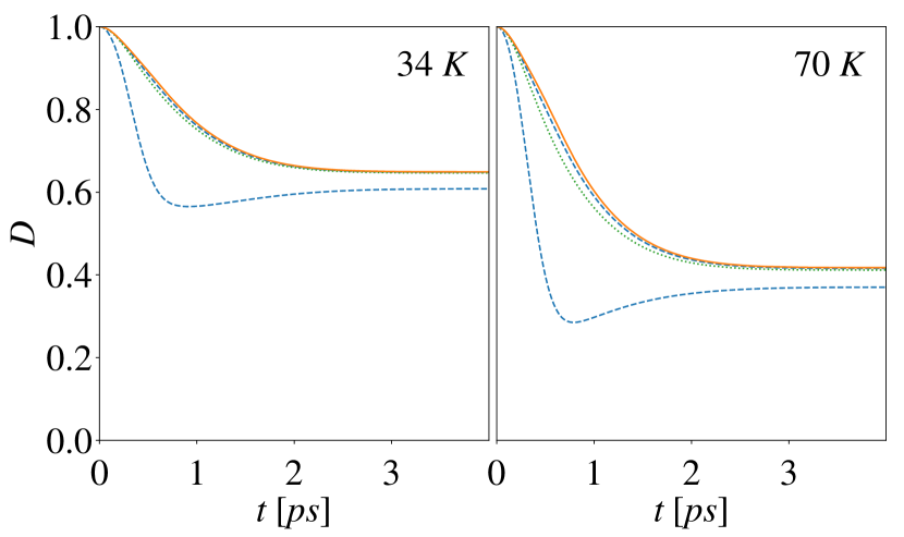
(b) $\tau_{MIN/MAX}\approx 0.42$ ps.

Figure 3: Degree of coherence as a function of time elapsed from the measurement $t$ at $T=34$ K (left plots) and $T=70$ K (right plots) for long delay times $\tau\approx 4$ ps (top panels) and $\tau\approx 0.42$ ps (bottom panels). Dashed lines correspond to points of maximal and minimal gain, while solid lines correspond to points of equal gain. Dotted lines are standard decoherence curves.

Fig. 2 shows the corresponding average gain of coherence (18) normalized by coherence which would be left in the system at time $t$ during the stnadard decoherence process, $g_{av}^{\prime}(\tau,t)=g_{av}(\tau,t)/(1-D(t))$, yielding a percentage of coherence gained. This is plotted at a long decoherence time $t=20$ ns, so all phonon-induced processes on the qubit have been finalized. In case of the system under study, the reservoir is super-Ohmic, which leads to $1-D(t)$ being fixed at a finite value; only at infinite temperature can complete decohrence be obtained [49, 52, 53, 45].

Figure 4: Function $G(k)$ for continuous phonon spectrum and the 19 phonon modes chosen in the discretization. Bars corresponding to each mode $k_{i}$ have width $\Delta k$.

The top panel of Fig. 2 again shows the envelope functions of $g_{av}^{\prime}(\tau,t)$ (the fast oscillations resulting from the large value of $\Delta\varepsilon$ are shown in the bottom panel for large delay times, around $\tau=4$ ps) at two temperatures. A saturation of the curves can be observed around $3.5$ ps, which corresponds well to the time-scales at which charge carrier-phonon processes occur in such systems. At later times the minimum value of the coherence gain is zero, because the non-classical phase factors are effectively zero and the expectation values of the environmental operators are no longer affected by their lack of commutation. The inset shows the short-time evolution when the minimum envelope curves are both below zero due to the non-classical phase factors which are relevant at such times. Note, that for very short times, both the minimum and maximum curves are below zero, so a loss of coherence is seen regardless of the fast oscillations between these curves.

To give the full picture of the phenomenon under study in Fig. 3 we present the degree of coherence as a function of time that elapsed from the intermediate measurement, $t$. In the upper panels, the curves correspond to $\tau\approx 4$ ps, which is well beyond the phonon relaxation times. The actual delay times for the three curves correspond to the points of maximal, minimal, and equal gain, which are closest to $4$ ps. Since the envelope functions change slowly in comparison to the oscillatory behavior driven by the energy difference between the qubit states, these curves can be freely compared. The time evolutions of the decoherence strongly resemble standard evolution (dotted lines) with the exception of a maximum/minimum which is present at $t\approx\tau$. This can be understood with the help of eq. (III.2) which holds for commuting operators $\hat{w}_{i}$, where decoherence is cancelled in one of the terms at $t=\tau$, yielding an extreme effect (either positive or negative, depending on the measurement outcome) on the degree of coherence.

The bottom panels show plots corresponding to the top panels, but at short delay times $\tau\approx 0.42$ corresponding to the minimum values in the inset of Fig. 2. The time evolutions are qualitatively different, firstly because the curves corresponding to the points of maximum and equal gain are almost identical to the standard decoherence decay, and the only distinct evolutions are the ones for the point of minimum gain (which are here always related to a loss). Furthermore, only these curves display any distinct behavior at $t=\tau$, which is a minimum, much less distinct than in the case of the evolutions corresponding to long delay times $\tau$.

IV.2 Discrete phonon spectrum

In this subsection we focus on a situation, in which the quantum dot interacts with a finite number of phonon modes, corresponding to the situation when the phonons are confined to a small structure and cannot be treated as those propagating within a bulk crystal [51]. To obtain qubit evolutions of a similar magnitude and occuring on similar time-scales as in the previous section, we will not model a specific medium for the phonons, but instead artificially “quantize” the phonon spectrum in terms of the phonon wave number, $k=|\pmb{k}|$.

This procedure is illustrated in Fig. 4, where the continuous line shows the $k$-dependence of $G(k)$, which is defined by the equation $H=\sum_{\pmb{k}}|\frac{f_{\pmb{k}}}{\omega_{\pmb{k}}}|^{2}=\int_{0}^{\infty}G(k)$ using the parameters from the previous subsection (IV.1) and is explicitly given by

$$G(k) = \frac{NV}{(2\pi)^{2}}\frac{(\sigma_{e}-\sigma_{h})^{2}}{2\rho c^{3}}k\int_{0}^{\pi}\,d\Theta sin\Theta$$ (38)

$$\times\exp[-\frac{1}{2}(l_{z}^{2}k^{2}\cos^{2}\Theta+l_{\perp}^{2}k^{2}\sin^{2}\Theta)].$$

Here the integration over the azimuthal angle has been performed and only the integration over the polar angle remains. We then choose $19$ equally spaced values of the wave number $k_{i}$ with $i=0,1,\dots,18$, where $k_{1}$ corresponds to the maximum of $G(k)$ and $\Delta k=k_{i+1}-k_{i}=2/3k_{1}=0.1282$ nm^-1, which means that the $k=0$ mode is taken into account with $G(k=0)=0$. We can now find $H_{i}=|\frac{f_{k_{i}}}{\omega_{k_{i}}}|^{2}=G(k_{i})\Delta k$ and the corresponding values of the coupling constants $f_{k_{i}}=\omega_{k_{i}}\sqrt{H_{i}}$ which enter eqs (35). This allows for all of the relevant quantities for the scheme under study to be found after replacing the integration over the wave vector $\pmb{k}$ with a summation over wave numbers $k_{i}$. In fact, only the particular values of $H_{i}$ and the corresponding energies $\omega_{k_{i}}$, with $\omega_{k_{i}}=ck_{i}$ under linear dispersion, are necessary to find the evolution of the degree of coherence both for standard decoherence and when the decoherence reduction scheme is used. Note that $H/\sum_{i}H_{i}=1.0176$ so that the bars in fig. 4 represent the function very well.

Figure 5: Envelope functions of the average gain of coherence: dependence on delay time $\tau$ at long $t=20$ ps for selected discrete sets of phonon wave numbers $k$. Environment with a single phonon mode: a) $k=k_{1}$ and b) $k=k_{10}$. More environmental modes: c) two phonon modes, $k_{0}$ and $k_{1}$, c) eleven phonon modes $k_{i}$, $i=0,\dots,10$.

Fig. 5 shows the $\tau$-dependence of the average gain of coherence for $t=20$ ps analogous to Fig. 2, but for a choice of wave numbers out of the 19 specified in Fig. 4 and described above. The coupling strengths are always adjusted, so that $\sum_{i}H_{i}=H$. When only a few phonon modes are taken into account (a,b,c), the evolution is highly periodic and the minima of the coherence gain display large negative values (especially in comparison with all that is observed in the case of the continuous spectrum). The recurring negativity is due to the fact that the effective cancellation of the non-commutativity of the operators (35) is connected with the interplay of many phonon modes when the spectrum approaches continuum. Note that this effect is obtained already for 10 phonon modes, as seen in fig. 5 (d). For smaller systems such cancellation cannot occur and the non-classical phases which lead to negative values of the coherence gain are much larger.

The top panels contain evolutions resulting from an interaction with only a single phonon mode, $k=k_{1}$ (a) and $k=k_{10}$ (b). Due to the adjustment of the coupling strength, they both interact similarly with the qubit and one can observe a change of periodicity of the evolution which is the result of the different energies of the two phonon modes, $\omega_{k_{i}}$. Qualitatively, the evolution is very similar, displaying two maxima of different magnitude and a minimum in each period. The differences are strongly visible in the gain and loss which can be achieved in the two cases. The reason for these differences lies in the arbitrary choice of the constant time $t$. Since both evolutions are periodic, but with a different periodicity, the interplays of times $t$ and $\tau$ are different in the two cases, yielding one evolution which is more favorable and has a high maximum gain, and one which is much worse in terms of coherence gain and a lot of the time leads to loss.

Adding a second phonon mode as in fig. 5 (c) leads to an expectedly more complicated evolution with three maxima an two minima in a single period, whereas the initial evolution is still dominated by the $k_{1}$ mode. With each additional mode this trend continues simultaneously extending the period of the evolution. Already at 10 modes (d), the losses of coherence become negligible in comparison to the situation when only a few modes are present and the tendency toward decoherence stabilizing at a finite value is demonstrated. This value is similar as in in the continuous spectrum case, Fig. 2, but a strong maximum characteristic for few-mode evolutions is still present. At 19 phonon modes, the evolution is of the same character as in fig. 5 (d).

V Conclusion

We have generalized the scheme for the reduction of decoherence introduced for a charge qubit interacting with a phononic bath [1] to the case of all qubit-environment interactions that lead to pure decoherence of the qubit. In this framework, we have shown that the scheme will always result in gain of coherence on average (over two outcomes of the qubit measurement which is the core of the scheme) if a mixture of environmental states $1/2[\hat{R}_{00}(\tau)+\hat{R}_{11}(\tau)]$ leads to the same decoherence curves as the initial environmental state $\hat{R}(0)$. The density matrices $\hat{R}_{ii}(\tau)$ correspond to environmental states which would be obtained from the initial state $\hat{R}(0)$ if the environment interacted with the qubit in state $|i\rangle$ for time $\tau$.

Such a situation is most commonly encountered when the operators that govern the evolution of the environment conditional on the pointer state of the qubit $|i\rangle$, commute. This is usually the outcome of commutation between different parts of the Hamiltonian, responsible for the distinguishability of qubit states by the environment. Another possibility is when the conditional environmental evolution operators do not commute with each other, but do commute with the initial state of the environment. For mixed states, this does not exclude decoherence, even though it excludes the formation of qubit-environment entanglement [8]. An example here is the infinite-temperature density matrix, which commutes with any evolution operator, and typically yields the strongest decoherence.

We observe this type of behavior in our example of a charge qubit coupled to an environment of phonons only for a continuous phonon spectrum and at long times, both the time of measurement and the time elapsed afterwards. At finite temperatures, this system does not fulfill any of the commutation relations specified in the previous paragraph, but nevertheless displays only gain of coherence and no loss. This is because at long times the non-trivial phase oscillations, which are the outcome of the lack of commutations, cancel out due to large-system effects. Hence, there are more situations where loss of coherence is unlikely, which are typically connected with more classical properties of the environment.

Situations when loss of coherence is observed are of more fundamental interest since they are only possible when the conditional evolution operators of the environment, and consequently observables which correspond to different parts of the Hamiltonian, do not commute. Hence, negative average gain of coherence is a witness of quantumness of the Hamiltonian and of the evolution of the environment, even though it does not have to be accompanied by qubit-environment entanglement at time $\tau$ [when $\hat{R}_{00}(\tau)=\hat{R}_{11}(\tau)<\hat{R}(0)$].

We observe very small losses of coherence at small times for the continuous spectrum example, but it is very common for a small and discrete number of phonon modes. Although for examples chosen in such a way that the same mode dominates the spectrum in the continuous and discrete case, observed losses of coherence are small and gain is more probable, we were able to find situations when the gain is predominantly negative.

Overall, we have shown that the scheme for pure decoherence control is of much wider usage than only for phonon-induced decoherence, as it is able to slow or reduce decoherence for a large class of interactions that lead to pure decoherence. In other cases (when loss of coherence on average is possible at certain measurement times $\tau$), it can still be used for decoherence control if time of measurement can be controlled with some reliability.

Code avaliability

All code used to generate plots in Sec. IV is available at https://github.com/brzepkowski/coherence_gain.

References

- Roszak et al. [2015] K. Roszak, R. Filip, and T. Novotný, Decoherence control by quantum decoherence itself., Scientific Reports 5, 9796 (2015).
- Borri et al. [2001] P. Borri, W. Langbein, S. Schneider, U. Woggon, R. L. Sellin, D. Ouyang, and D. Bimberg, Ultralong dephasing time in ingaas quantum dots, Phys. Rev. Lett. 87, 157401 (2001).
- Krummheuer et al. [2002] B. Krummheuer, V. M. Axt, and T. Kuhn, Theory of pure dephasing and the resulting absorption line shape in semiconductor quantum dots, Phys. Rev. B 65, 195313 (2002).
- Vagov et al. [2004] A. Vagov, V. M. Axt, T. Kuhn, W. Langbein, P. Borri, and U. Woggon, Nonmonotonous temperature dependence of the initial decoherence in quantum dots, Phys. Rev. B 70, 201305 (2004).
- Vagov et al. [2006] A. Vagov, M. D. Croitoru, V. M. Axt, T. Kuhn, and F. M. Peeters, High pulse area undamping of rabi oscillations in quantum dots coupled to phonons, physica status solidi (b) 243, 2233 (2006) .
- Mermillod et al. [2016] Q. Mermillod, D. Wigger, V. Delmonte, D. E. Reiter, C. Schneider, M. Kamp, S. Höfling, W. Langbein, T. Kuhn, G. Nogues, and J. Kasprzak, Dynamics of excitons in individual inas quantum dots revealed in four-wave mixing spectroscopy, Optica 3, 377 (2016).
- Wigger et al. [2018] D. Wigger, C. Schneider, S. Gerhardt, M. Kamp, S. Höfling, T. Kuhn, and J. Kasprzak, Rabi oscillations of a quantum dot exciton coupled to acoustic phonons: coherence and population readout, Optica 5, 1442 (2018).
- Roszak and Cywiński [2015] K. Roszak and L. Cywiński, Characterization and measurement of qubit-environment-entanglement generation during pure dephasing, Phys. Rev. A 92, 032310 (2015).
- Rzepkowski and Roszak [2021] B. Rzepkowski and K. Roszak, A scheme for direct detection of qubit–environment entanglement generated during qubit pure dephasing, Quantum Information Processing 20, 1 (2021).
- Roszak and Cywiński [2018] K. Roszak and L. Cywiński, Equivalence of qubit-environment entanglement and discord generation via pure dephasing interactions and the resulting consequences, Phys. Rev. A 97, 012306 (2018).
- Ollivier and Zurek [2002] H. Ollivier and W. H. Zurek, Quantum Discord: A Measure of the Quantumness of Correlations, Physical Review Letters 88, 017901 (2002) .
- Modi et al. [2012] K. Modi, A. Brodutch, H. Cable, T. Paterek, and V. Vedral, The classical-quantum boundary for correlations: Discord and related measures, Reviews of Modern Physics 84, 1655 (2012).
- Modi [2014] K. Modi, A pedagogical overview of quantum discord, Open Systems & Information Dynamics 21, 1440006 (2014).
- Salamon and Roszak [2017] T. Salamon and K. Roszak, Entanglement generation between a charge qubit and its bosonic environment during pure dephasing: Dependence on the environment size, Phys. Rev. A 96, 032333 (2017).
- Strzałka et al. [2020] M. Strzałka, D. Kwiatkowski, L. Cywiński, and K. Roszak, Qubit-environment negativity versus fidelity of conditional environmental states for a nitrogen-vacancy-center spin qubit interacting with a nuclear environment, Phys. Rev. A 102, 042602 (2020).
- Pernice and Strunz [2011] A. Pernice and W. T. Strunz, Decoherence and the nature of system-environment correlations, Phys. Rev. A 84, 062121 (2011).
- Lo Franco et al. [2012] R. Lo Franco, B. Bellomo, E. Andersson, and G. Compagno, Revival of quantum correlations without system-environment back-action, Phys. Rev. A 85, 032318 (2012).
- Szańkowski et al. [2017] P. Szańkowski, G. Ramon, J. Krzywda, D. Kwiatkowski, and L. Cywiński, Environmental noise spectroscopy with qubits subjected to dynamical decoupling, Journal of Physics: Condensed Matter 29, 333001 (2017).
- Chen et al. [2018] H.-B. Chen, C. Gneiting, P.-Y. Lo, Y.-N. Chen, and F. Nori, Simulating open quantum systems with hamiltonian ensembles and the nonclassicality of the dynamics, Phys. Rev. Lett. 120, 030403 (2018).
- Wenderoth et al. [2021] S. Wenderoth, H.-P. Breuer, and M. Thoss, Non-markovian effects in the spin-boson model at zero temperature, Phys. Rev. A 104, 012213 (2021).
- Chruściński et al. [2022] D. Chruściński, S. Hesabi, and D. Lonigro, On markovianity and classicality in multilevel spin-boson models (2022), arXiv:2210.06199 [quant-ph] .
- Cywiński et al. [2009] Ł. Cywiński, W. M. Witzel, and S. Das Sarma, Pure quantum dephasing of a solid-state electron spin qubit in a large nuclear spin bath coupled by long-range hyperfine-mediated interactions, Phys. Rev. B 79, 245314 (2009).
- Paladino et al. [2014] E. Paladino, Y. M. Galperin, G. Falci, and B. L. Altshuler, 1/f noise: Implications for solid-state quantum information, Rev. Mod. Phys. 86, 361 (2014).
- Wu et al. [2018] Y. Wu, L.-P. Yang, M. Gong, Y. Zheng, H. Deng, Z. Yan, Y. Zhao, K. Huang, A. D. Castellano, W. J. Munro, et al., An efficient and compact switch for quantum circuits, npj Quantum Information 4, 1 (2018).
- Touzard et al. [2019] S. Touzard, A. Kou, N. E. Frattini, V. V. Sivak, S. Puri, A. Grimm, L. Frunzio, S. Shankar, and M. H. Devoret, Gated conditional displacement readout of superconducting qubits, Phys. Rev. Lett. 122, 080502 (2019).
- Campagne-Ibarcq et al. [2020] P. Campagne-Ibarcq, A. Eickbusch, S. Touzard, E. Zalys-Geller, N. E. Frattini, V. V. Sivak, P. Reinhold, S. Puri, S. Shankar, R. J. Schoelkopf, et al., Quantum error correction of a qubit encoded in grid states of an oscillator, Nature 584, 368 (2020).
- Wood et al. [2018] A. A. Wood, E. Lilette, Y. Y. Fein, N. Tomek, L. P. McGuinness, L. C. L. Hollenberg, R. E. Scholten, and A. M. Martin, Quantum measurement of a rapidly rotating spin qubit in diamond, Science Advances 4, 368 (2018).
- Tchebotareva et al. [2019] A. Tchebotareva, S. L. N. Hermans, P. C. Humphreys, D. Voigt, P. J. Harmsma, L. K. Cheng, A. L. Verlaan, N. Dijkhuizen, W. de Jong, A. Dréau, and R. Hanson, Entanglement between a diamond spin qubit and a photonic time-bin qubit at telecom wavelength, Phys. Rev. Lett. 123, 063601 (2019).
- Wang et al. [2020] X. Wang, Y. Xiao, C. Liu, E. Lee-Wong, N. J. McLaughlin, H. Wang, M. Wu, H. Wang, E. E. Fullerton, and C. R. Du, Electrical control of coherent spin rotation of a single-spin qubit, npj Quantum Information 6, 1 (2020).
- Watzinger et al. [2018] H. Watzinger, J. Kukučka, L. Vukušić, F. Gao, T. Wang, F. Schäffler, J.-J. Zhang, and G. Katsaros, A germanium hole spin qubit, Nature communications 9, 1 (2018).
- Hendrickx et al. [2020] N. Hendrickx, W. Lawrie, L. Petit, A. Sammak, G. Scappucci, and M. Veldhorst, A single-hole spin qubit, Nature communications 11, 1 (2020).
- Miao et al. [2020] K. C. Miao, J. P. Blanton, C. P. Anderson, A. Bourassa, A. L. Crook, G. Wolfowicz, H. Abe, T. Ohshima, and D. D. Awschalom, Universal coherence protection in a solid-state spin qubit, Science 369, 1493 (2020).
- Madzik et al. [2021] M. T. Madzik, A. Laucht, F. E. Hudson, A. M. Jakob, B. C. Johnson, D. N. Jamieson, K. M. Itoh, A. S. Dzurak, and A. Morello, Conditional quantum operation of two exchange-coupled single-donor spin qubits in a mos-compatible silicon device, Nature communications 12, 1 (2021).
- Fricke et al. [2021] L. Fricke, S. J. Hile, L. Kranz, Y. Chung, Y. He, P. Pakkiam, M. G. House, J. G. Keizer, and M. Y. Simmons, Coherent control of a donor-molecule electron spin qubit in silicon, Nature communications 12, 1 (2021).
- Roszak and Cywiński [2021] K. Roszak and L. Cywiński, Qubit-environment-entanglement generation and the spin echo, Phys. Rev. A 103, 032208 (2021).
- Roszak et al. [2019] K. Roszak, D. Kwiatkowski, and L. Cywiński, How to detect qubit-environment entanglement generated during qubit dephasing, Phys. Rev. A 100, 022318 (2019).
- Strzałka and Roszak [2021] M. Strzałka and K. Roszak, Detection of entanglement during pure dephasing evolutions for systems and environments of any size, Phys. Rev. A 104, 042411 (2021).
- Harlender and Roszak [2022] T. Harlender and K. Roszak, Transfer and teleportation of system-environment entanglement, Phys. Rev. A 105, 012407 (2022).
- Roszak and Korbicz [2022] K. Roszak and J. K. Korbicz, Purifying teleportation (2022), arXiv:2208.13545 [quant-ph] .
- Roszak [2018] K. Roszak, Criteria for system-environment entanglement generation for systems of any size in pure-dephasing evolutions, Phys. Rev. A 98, 052344 (2018).
- Chen et al. [2019] H.-B. Chen, P.-Y. Lo, C. Gneiting, J. Bae, Y.-N. Chen, and F. Nori, Quantifying the nonclassicality of pure dephasing, Nature Comm. 10, 3794 (2019).
- Popovic et al. [2021] M. Popovic, M. T. Mitchison, and J. Goold, Thermodynamics of decoherence (2021), arXiv:2107.14216 [quant-ph] .
- Zurek [2003] W. H. Zurek, Decoherence, einselection, and the quantum origins of the classical, Rev. Mod. Phys. 75, 715 (2003).
- Roszak and Korbicz [2019] K. Roszak and J. K. Korbicz, Entanglement and objectivity in pure dephasing models, Phys. Rev. A 100, 062127 (2019).
- Tuziemski et al. [2019] J. Tuziemski, A. Lampo, M. Lewenstein, and J. K. Korbicz, Reexamination of the decoherence of spin registers, Phys. Rev. A 99, 022122 (2019).
- Lambert et al. [2019] N. Lambert, S. Ahmed, M. Cirio, and F. Nori, Modelling the ultra-strongly coupled spin-boson model with unphysical modes, Nature communications 10, 1 (2019).
- Miessen et al. [2021] A. Miessen, P. J. Ollitrault, and I. Tavernelli, Quantum algorithms for quantum dynamics: A performance study on the spin-boson model, Phys. Rev. Research 3, 043212 (2021).
- Michaelis de Vasconcellos et al. [2010] S. Michaelis de Vasconcellos, S. Gordon, M. Bichler, T. Meier, and A. Zrenner, Coherent control of a single exciton qubit by optoelectronic manipulation, Nature Photonics 4, 545 (2010).
- Leggett et al. [1987] A. J. Leggett, S. Chakravarty, A. T. Dorsey, M. P. A. Fisher, A. Garg, and W. Zwerger, Dynamics of the dissipative two-state system, Rev. Mod. Phys. 59, 1 (1987).
- Roszak and Machnikowski [2006] K. Roszak and P. Machnikowski, “which path” decoherence in quantum dot experiments, Physics Letters A 351, 251 (2006).
- Mahan [2000] G. D. Mahan, Many-Particle Physics (Kluwer, New York, 2000).
- An and Zhang [2007] J.-H. An and W.-M. Zhang, Non-markovian entanglement dynamics of noisy continuous-variable quantum channels, Phys. Rev. A 76, 042127 (2007).
- Hu and Fan [2012] M.-L. Hu and H. Fan, Quantum-memory-assisted entropic uncertainty principle, teleportation, and entanglement witness in structured reservoirs, Phys. Rev. A 86, 032338 (2012).