Next-to-leading-power kinematic corrections to DVCS:
a scalar target

Abstract

Using the recent results on the contributions of descendants of the leading twist operators to the operator product expansion of two electromagnetic currents we derive explicit expressions for the kinematic finite-$t$ and target mass corrections to the DVCS helicity amplitudes to the $1/Q^{4}$ power accuracy. The cancellation of IR divergences for kinematic corrections is demonstrated to all powers in the leading order of perturbation theory. We also argue that target mass corrections in the coherent DVCS from nuclei are small and do not invalidate the factorization theorem.

1 Introduction

A three-dimensional “tomographic” imaging of the proton and light nuclei is an active research topic and a major science goal for the planned Electron-Ion Collider (EIC) AbdulKhalek:2021gbh ; AbdulKhalek:2022erw . Studies of the deeply-virtual Compton scattering (DVCS) play an important role in this undertaking. This reaction gives access to the generalized parton distributions (GPDs) Muller:1994ses ; Ji:1996nm ; Radyushkin:1997ki that encode the information on the transverse position of quarks and gluons in the proton in dependence on their longitudinal momentum. This process will be measured with very high precision and in a broad kinematic range. The QCD description of the DVCS is based on collinear factorization with GPDs as nonperturbative inputs and coefficient functions (CFs) which can be calculated order by order in perturbation theory. At leading power, the complete next-to-leading-order (NLO) results are available since many years Ji:1998xh ; Belitsky:1999hf ; Belitsky:1998gc ; Noritzsch:2003un , and the work is ongoing to extend this description to NNLO Kumericki:2006xx ; Kumericki:2007sa ; Braun:2017cih ; Braun:2020yib ; Braun:2021grd ; Gao:2021iqq ; Braun:2022byg ; VanThurenhout:2022hgd ; Braun:2022bpn .

Beyond the leading twist, power-suppressed contributions $\sim(\sqrt{-t}/Q)^{k}$ and $\sim(m/Q)^{k}$ where $t$ is the invariant momentum transfer and $m$ is the target mass, have to be taken into account. The spatial position of partons is Fourier conjugate to the momentum transfer to the nucleon in the scattering process. Hence the resolving power of DVCS is directly limited by the range of the invariant moment transfer $t$ available in the analysis. For the stated goal of the three-dimensional imaging, theoretical control over power corrections $(\sqrt{-t}/Q)^{k}$ is therefore of paramount importance. Another pressing issue is to clarify whether target mass corrections do not invalidate QCD factorization for coherent DVCS on nuclei CLAS:2017udk ; CLAS:2021ovm .

An intuitive way to understand the meaning and importance of kinematic power corrections is the following Braun:2014paa . The leading-twist approximation in DVCS is intrinsically ambiguous since the four-momenta of the initial and final photons and protons do not lie in one plane. Hence the distinction of longitudinal and transverse directions is convention-dependent. In the Bjorken high-energy limit this is the $1/Q$ effect. The freedom to redefine large “plus” parton momenta by adding smaller transverse components has two consequences. First, the relation of the skewness parameter $\xi$ with the Bjorken variable $x_{B}$ may involve power suppressed contributions. Second, such a redefinition generally leads to excitation of the subleading photon helicity-flip amplitudes Braun:2014sta ; Braun:2014paa . This convention-dependence should be viewed as a theoretical uncertainty and is numerically rather large, see Guo:2021gru for a detailed study.

At the present time, the kinematic power corrections to DVCS are known to the twist-four accuracy, i.e. up to terms $\sim t/Q^{2}$ and $\sim m^{2}/Q^{2}$ Braun:2014sta . A typical size of these corrections is of order 10% for asymmetries, but they can be as large as 100% for the cross section in certain kinematics. These corrections can significantly impact the extraction of GPDs from data and have to be taken into account Defurne:2015kxq ; Defurne:2017paw . The formalism of Refs. Braun:2012bg ; Braun:2014sta was used in the most recent study by the JLAB Hall A collaboration JeffersonLabHallA:2022pnx . This publication presents the first experimental extraction of all four helicity-conserving Compton Form Factors (CFFs) of the nucleon as a function of $x_{B}$, while systematically including higher-twist helicity flip amplitudes in the kinematic approximation. It is argued that helicity-flip amplitudes contribute to producing a good fit of the cross section and most importantly to providing realistic uncertainties on the helicity-conserving CFFs. The helicity-conserving contribution alone overshoots the data at 180 degrees scattering angle, which is then compensated by helicity-flip contributions .

Our aim is to develop an approach that would allow one to calculate and possibly resum the corrections $\sim(\sqrt{-t}/Q)^{k}$ and $\sim(m/Q)^{k}$ to all powers. On a more formal level, the task can be formulated as follows. Let $\mathcal{O}^{\mu_{1}\ldots\mu_{N}}$ be local twist-two operators. The matrix elements of these operators define the GPD moments. The kinematic contributions we are considering here receive contributions of higher-twist descendants of the twist-two operators, of the type

$$\partial_{\mu_{1}}\mathcal{O}^{\mu_{1}\mu_{2}\ldots\mu_{N}},\qquad\partial_{\mu_{1}}\partial_{\mu_{2}}\mathcal{O}^{\mu_{1}\mu_{2}\mu_{3}\ldots\mu_{N}},\qquad\partial^{2}\mathcal{O}^{\mu_{1}\ldots\mu_{N}},\quad\text{etc.},$$ (1)

where $\partial_{\mu}$ is a total derivative. The problem is that matrix elements of the first two operators in (1) (and similar ones with more derivatives) vanish for on-mass-shell partons. Hence the usual method to calculate the OPE coefficients functions for these operators — evaluate both sides of the OPE on free quarks — is not applicable. The technique developed in Braun:2011zr ; Braun:2011dg ; Braun:2012bg ; Braun:2012hq is based on considering instead quark-antiquark-gluon matrix elements and using symmetry properties of the corresponding renormalization group equations. Unfortunately this approach becomes too unwieldy beyond twist four.

In Ref. Braun:2020zjm we suggested a different technique based on the conformal field theory (CFT) methods. In a conformal theory, the coefficients with which the descendant operators enter the OPE are completely determined by the leading-twist contributions that can be obtained by considering forward matrix elements Ferrara:1971vh ; Ferrara:1971zy ; Ferrara:1973yt . For QCD, this means that kinematic corrections to DVCS amplitudes are unambiguously determined by DIS coefficient functions. Of course, QCD is not a conformal theory. However, one can consider a modified theory, QCD in non-integer $d=4-2\epsilon$ space-time dimensions and fine-tune the strong coupling $\alpha_{s}$ to nullify the $\beta$-function (Wilson-Fisher fixed point Wilson:1973jj ). This restores the scale and conformal invariance of the correlation functions of gauge-invariant operators Braun:2018mxm . Observables calculated in the four-dimensional and critical QCD differ beyond leading order by terms proportional to the QCD $\beta$ function. Such terms can be calculated and added, at least in principle Braun:2020yib , while there are no corrections at the tree level.

The OPE for the product of two conserved vector currents in a generic CFT was constructed in Ref. Braun:2020zjm . The expansion for the product of two scalar currents was originally obtained in Ref. Ferrara:1971vh in a different form. A simple representation for the coefficient functions obtained in Braun:2020zjm is well-suited for studies of high-energy scattering in QCD (possible applications beyond DVCS include the studies of $t$-channel processes like $\gamma^{\ast}\gamma\to\pi\pi$, see Lorce:2022tiq ).

In this work we use this result to calculate the finite-$t$ and target mass corrections to the helicity amplitudes in DVCS on a scalar target to the next-to-leading power accuracy and the leading order in the strong coupling. Schematically,

$$\mathcal{A}^{++} \sim 1+\frac{1}{Q^{2}}+\frac{1}{Q^{4}}\,,$$

$$\mathcal{A}^{0+} \sim\frac{1}{Q}+\frac{1}{Q^{3}}\,,$$

$$\mathcal{A}^{-+} \sim\frac{1}{Q^{2}}+\frac{1}{Q^{4}}\,,$$ (2)

where $\mathcal{A}^{++}$, $\mathcal{A}^{0+}$ and $\mathcal{A}^{-+}$ are the helicity-conserving, helicity-flip and double-helicity-flip amplitudes, respectively, in a particular reference frame Braun:2012bg . Precise definitions are given in the text. An extension to higher powers is straightforward but unlikely to be relevant for phenomenology, so that we do not work out explicit expressions.

In Section 2 we carry out the first part of this program. Namely, we rewrite the OPE obtained in Ref. Braun:2020zjm in terms of the nonlocal light-ray operators. To this end we develop a certain technique which relies heavily on the representation theory of $\mathrm{SU}(1,1)$ group. The light-ray OPE in Eq. (2.2.3) presents the final result for this part.

Matrix elements of light-ray operators are defined in terms of the GPDs. Thus the Fourier transformation of the expression obtained in Section 2 yields helicity amplitudes for the DVCS on a chosen target. This calculation is described in Section 3. It is straightforward but proves to be very cumbersome. We find that individual contributions contain infrared (IR) singularities that cancel in the sum to all orders in the power expansion. We also find that the singularities of the coefficient functions at the kinematic point $x=\xi$ do not become stronger to all powers, so that the collinear factorization is not endangered. We work our explicit expressions for the kinematic power corrections to the accuracy indicated in Eq. (2) and show that target mass corrections are not enhanced for nuclear targets. Taking into account these corrections removes the frame dependence of the leading-twist approximation and restores the electromagnetic gauge invariance of the Compton amplitude up to $1/Q^{5}$ effects. The final Section 4 contains a short numerical study, our conclusions and outlook. Some more technical details are given in the Appendices.

2 Light-ray operator product expansion

Our starting expression in this paper is the result of Ref. Braun:2020zjm for the OPE of two electromagnetic currents taking into account contributions of leading-twist operators and their higher-twist descendants, cf. Eq. (1)

$$\mathrm{T}\{j^{\mu}(x_{1})j^{\nu}(x_{2})\} =\frac{1}{i\pi^{2}}\!\!\sum_{N>0,\text{even}}\!\frac{\rho_{N}}{N\!+\!1}\int_{0}^{1}\!du\,(u\bar{u})^{N}\Biggl{\{}\frac{1}{(-x_{12}^{2}+i0)^{2}}\Biggl{[}(N+1)g^{\mu\nu}\biggl{(}1-\frac{1}{4}\frac{u\bar{u}}{N+1}{x_{12}^{2}}\partial^{2}\biggr{)}$$

$$\quad+\frac{1}{2N}x_{12}^{2}\big{(}\partial_{1}^{\mu}\partial_{2}^{\nu}-\partial_{1}^{\nu}\partial_{2}^{\mu}\big{)}+\left(1-\frac{u\bar{u}}{N}\frac{x_{12}^{2}\partial^{2}}{4}\right)\left(\frac{\bar{u}}{u}x_{21}^{\mu}\partial_{1}^{\nu}+\frac{u}{\bar{u}}x_{12}^{\nu}\partial_{2}^{\mu}\right)$$

$$\quad-\frac{u\bar{u}}{N(N\!+\!1)}\frac{x_{12}^{2}\partial^{2}}{4}\Big{(}x_{21}^{\nu}\partial_{1}^{\mu}\!+\!x_{12}^{\mu}\partial_{2}^{\nu}\Big{)}-\frac{x_{12}^{\mu}x_{12}^{\nu}}{N\!+\!1}u\bar{u}\partial^{2}\biggl{(}\!1-\frac{u\bar{u}}{N\!+\!2}\frac{x_{12}^{2}\partial^{2}}{4}\biggr{)}\Biggr{]}\mathcal{O}^{(0)}_{N}\!(x_{21}^{u})$$

$$\quad-\frac{1}{(-x_{12}^{2}+i0)}\Biggl{[}-\frac{1}{4}N(\bar{u}-u)\,g^{\mu\nu}-\frac{\bar{u}-u}{4(N+1)}\big{(}x_{21}^{\nu}\partial_{1}^{\mu}+x_{12}^{\mu}\partial_{2}^{\nu}\big{)}$$

$$\quad+\frac{1}{2}\Big{(}\bar{u}\,x_{21}^{\mu}\partial_{1}^{\nu}-u\,x_{12}^{\nu}\partial_{2}^{\mu}\Big{)}+\frac{N}{2(N+2)(N-1)}\Big{(}x_{21}^{\nu}\partial_{1}^{\mu}-x_{12}^{\mu}\partial_{2}^{\nu}\Big{)}$$

$$\quad+\frac{1}{4}\frac{N(N^{2}+N+2)}{(N+1)(N+2)(N-1)}\left(\frac{u}{\bar{u}}x_{12}^{\nu}\partial_{2}^{\mu}-\frac{\bar{u}}{u}x_{21}^{\mu}\partial_{1}^{\nu}\right)$$

$$\quad+\frac{x_{12}^{\mu}x_{12}^{\nu}}{(-x_{12}^{2}+i0)}(\bar{u}-u)\frac{N}{N+1}\left(1-\frac{1}{2}\frac{u\bar{u}}{N+2}x_{12}^{2}\partial^{2}\right)\Biggr{]}\,\mathcal{O}^{(1)}_{N}(x_{21}^{u})$$ (3)

$$\quad-\frac{x_{12}^{\mu}x_{12}^{\nu}}{(-x_{12}^{2}+i0)}\!\left[\frac{N^{2}+N+2}{4(N+1)(N+2)}\!-\!\frac{u\bar{u}N(N-1)}{(N+1)(N+2)}\right]\mathcal{O}_{N}^{(2)}(x_{21}^{u})\Biggl{\}}\,+\ldots,$$

where

$$\rho_{N} =i^{N-1}\frac{(2N+1)!}{(N-1)!N!\,N!}\,,$$ (4)

$$\bar{u}=1-u\,,\qquad x_{12}=x_{1}-x_{2}\,,\qquad x_{21}^{u}=\bar{u}x_{2}+ux_{1}\,,\qquad\partial_{1}^{\mu}=\frac{\partial}{\partial x_{1}^{\mu}}\,,\qquad\partial_{2}^{\mu}=\frac{\partial}{\partial x_{2}^{\mu}}$$ (5)

and a derivative without a subscript $1,2$ stands for

$$\partial^{\mu}\mathcal{O}_{N}^{(k)}(y)=\frac{\partial}{\partial y_{\mu}}\mathcal{O}_{N}^{(k)}(y)\,.$$ (6)

For a generic hadronic matrix element between states with different momenta

$$\langle p^{\prime}|\partial^{\mu}\mathcal{O}_{N}^{(k)}(y)|p\rangle=i\Delta^{\mu}\langle p^{\prime}|\mathcal{O}_{N}^{(k)}(y)|p\rangle\,,\qquad\Delta^{\mu}=(p^{\prime}-p)^{\mu}\,,$$ (7)

so that in what follows we will often replace $\partial^{\mu}\mapsto i\Delta^{\mu}$, $\partial^{2}\mapsto-\Delta^{2}$ already on the operator level.

The operators $\mathcal{O}^{(k)}_{N}$ are defined as

$$\mathcal{O}^{(0)}_{N}(y) =x_{12,\mu_{1}}\cdots x_{12,\mu_{N}}\mathcal{O}_{N}^{\mu_{1}\ldots\mu_{N}}(y)\,,$$

$$\mathcal{O}^{(1)}_{N}(y) =x_{12,\mu_{2}}\cdots x_{12,\mu_{N}}\frac{\partial}{\partial y^{\mu_{1}}}\mathcal{O}_{N}^{\mu_{1}\ldots\mu_{N}}(y)\,,$$

$$\mathcal{O}^{(2)}_{N}(y) =x_{12,\mu_{3}}\cdots x_{12,\mu_{N}}\frac{\partial}{\partial y^{\mu_{1}}}\frac{\partial}{\partial y^{\mu_{2}}}\mathcal{O}_{N}^{\mu_{1}\ldots\mu_{N}}(y)\,,$$ (8)

where $\mathcal{O}_{N}^{\mu_{1}\ldots\mu_{N}}$ are multiplicatively renormalizable leading-twist operators with spin $N$ normalized as

$$\mathcal{O}_{N}^{\mu_{1}\ldots\mu_{N}}(0)=i^{N-1}\bar{q}(0)\gamma^{\{\mu_{1}}D^{\mu_{2}}\ldots D^{\mu_{N}\}}q(0)+\,\text{total~{}derivatives}\,.$$ (9)

Here $\{\ldots\}$ denotes symmetrization and trace subtraction for all enclosed Lorentz indices. In what follows we will use the notation $[\ldots]_{lt}$ for the leading-twist part of an operator, e.g.,

$$\big{[}\bar{q}(0)\gamma^{\mu_{1}}D^{\mu_{2}}\ldots D^{\mu_{N}}q(0)\big{]}_{lt}=\bar{q}(0)\gamma^{\{\mu_{1}}D^{\mu_{2}}\ldots D^{\mu_{N}\}}q(0)\,.$$ (10)

In the accepted normalization

$$n_{\mu_{1}}\ldots n_{\mu_{N}}\mathcal{O}_{N}^{\mu_{1}\ldots\mu_{N}}(y)=\frac{\Gamma(3/2)\Gamma(N)}{\Gamma(N+1/2)}\left(\frac{i\partial_{+}}{{4}}\right)^{N-1}\bar{q}(y)\gamma_{+}C_{N-1}^{3/2}\left(\tfrac{\stackrel{{\scriptstyle\rightarrow}}{{D}}_{+}-\stackrel{{\scriptstyle\leftarrow}}{{D}}_{+}}{\stackrel{{\scriptstyle\rightarrow}}{{D}}_{+}+\stackrel{{\scriptstyle\leftarrow}}{{D}}_{+}}\right)q(y)\,,$$ (11)

where $n^{\mu}$ is an arbitrary light-like vector, $n^{2}=0$, $D_{+}=D^{\mu}n_{\mu}$, etc. The expression in Eq. (2) satisfies exact electromagnetic Ward identities

$$\partial_{1}^{\mu}\mathrm{T}\{j^{\mu}(x_{1})j^{\nu}(x_{2})\}=\partial_{2}^{\nu}\mathrm{T}\{j^{\mu}(x_{1})j^{\nu}(x_{2})\}=0$$ (12)

up to, possibly, polynomials in $x_{12}^{2}$ which give rise to delta-function terms after Fourier transform to the momentum space. The OPE in this form is term-by term translation invariant (cf. a discussion in  Braun:2011zr ; Braun:2011dg )

$$\langle p^{\prime}|\mathrm{T}\{j^{\mu}(x_{1}+y)j^{\nu}(x_{2}+y)\}|p\rangle =e^{i(\Delta\cdot y)}\langle p^{\prime}|\mathrm{T}\{j^{\mu}(x_{1})j^{\nu}(x_{2})\}|p\rangle\,,$$ (13)

so that without loss of generality one can make a specific choice, e.g., consider $\mathrm{T}\{j^{\mu}(x)j^{\nu}(0)\}$ or $\mathrm{T}\{j^{\mu}(0)j^{\nu}(-x)\}$ to simplify the algebra.

2.1 Twist expansion

The conformal OPE in (2) involves leading-twist operators integrated with a certain weight function over their position on the straight line connecting the electromagnetic currents. Since the separation $x_{12}$ is not light-like, $x_{12}^{2}\not{=}0$, this integration upsets the twist expansion. Indeed, expanding $\mathcal{O}_{N}^{(0)}(x_{21}^{u})$, e.g., around the middle point $x_{21}^{\scriptscriptstyle u=1/2}=x^{+}=\frac{1}{2}(x_{1}+x_{2})$ one obtains local operators of the form

$$x_{12}^{\nu_{1}}\ldots x_{12}^{\nu_{k}}\,x_{12}^{\mu_{1}}\ldots x_{12}^{\mu_{N}}\partial_{\nu_{1}}\ldots\partial_{\nu_{k}}\bar{q}(x^{+})\gamma_{\{\mu_{1}}D_{\mu_{2}}\ldots D_{\mu_{N}\}}q(x^{+})\,,$$ (14)

where not all traces are subtracted. As the first step, we need to rewrite (2) in terms of the leading twist operators

$$\big{[}\partial_{\nu_{1}}\ldots\partial_{\nu_{k}}\bar{q}\gamma_{\mu_{1}}D_{\mu_{2}}\ldots D_{\mu_{N}}q\big{]}_{lt}=\partial_{\{\nu_{1}}\ldots\partial_{\nu_{k}}\bar{q}\gamma_{\mu_{1}}D_{\mu_{2}}\ldots D_{\mu_{N}\}}q\,.$$ (15)

This can be done retaining the structure of the conformal OPE using the technique of Refs. Balitsky:1987bk ; Balitsky:1990ck .

For simplicity, take $x_{1}=x$, $x_{2}=0$ so that $x_{21}^{u}=ux$. The leading twist projection of a function $f(x)$ satisfies the Laplace equation, $\partial_{x}^{2}[f(x)]_{lt}=0$, with the boundary condition $[f(x)]_{lt}=f(x)$ at $x^{2}=0$. The solution can be written as an expansion in powers of the deviation from the light cone Balitsky:1987bk

$$[f(x)]_{lt} =f(x)-\frac{1}{4}x^{2}\int_{0}^{1}\frac{dt}{t}\partial_{x}^{2}f(tx)+\frac{1}{32}x^{4}\int_{0}^{1}\frac{dt}{t}\frac{\bar{t}}{t}\partial_{x}^{4}f(tx)+\mathcal{O}(x^{6})\,.$$ (16)

The inverse relation reads

$$f(x) =[f(x)]_{lt}+\frac{1}{4}x^{2}\int_{0}^{1}\frac{dt}{t}[\partial_{x}^{2}f(tx)]_{lt}+\frac{1}{32}x^{4}\int_{0}^{1}dt\,\frac{\bar{t}}{t^{3}}[\partial_{x}^{4}\,f(tx)]_{lt}+\mathcal{O}(x^{6})\,.$$ (17)

Replacing $f(x)$ by $\mathcal{O}_{N}^{(0)}(ux)$ one obtains

$$\mathcal{O}^{(0)}_{N}(ux) =[\mathcal{O}^{(0)}_{N}(ux)]_{lt}+\frac{x^{2}}{4}\!\int_{0}^{1}\!\frac{dt}{t}\Big{[}\partial_{x}^{2}e^{iut\Delta x}t^{N}\mathcal{O}^{(0)}_{N}(0)\Big{]}_{lt}+\frac{x^{4}}{32}\!\int_{0}^{1}\!\frac{\bar{t}\,dt}{t^{3}}\partial_{x}^{4}\Big{[}e^{iut\Delta x}t^{N}\mathcal{O}^{(0)}_{N}(0)\Big{]}\!+\mathcal{O}(x^{6})$$

$$=[\mathcal{O}^{(0)}_{N}(ux)]_{lt}-\frac{x^{2}}{4}\int_{0}^{1}\frac{dt}{t}t^{N}\Big{[}u^{2}t^{2}\Delta^{2}[\mathcal{O}^{(0)}_{N}]_{lt}(utx)-2utN[\mathcal{O}^{(1)}_{N}]_{lt}(utx)\Big{]}$$

$$\quad+\frac{x^{4}}{32}\int_{0}^{1}\!dt\,\frac{\bar{t}}{t^{3}}t^{N}\biggl{\{}u^{4}t^{4}\Delta^{4}[\mathcal{O}^{(0)}_{N}(utx)]_{lt}-4Nu^{3}t^{3}\Delta^{2}[\mathcal{O}^{(1)}_{N}(utx)]_{lt}$$

$$\quad+4N(N-1)u^{2}t^{2}[\mathcal{O}^{(2)}_{N}(utx)]_{lt}\biggr{\}}+\mathcal{O}(x^{6})\,,$$ (18)

where taking the matrix element $\langle p^{\prime}|\ldots|p\rangle$ is tacitly assumed hence $(p^{\prime}-p)^{\mu}=\Delta^{\mu}\Leftrightarrow-i\partial^{\mu}$, and we used that $\partial_{x}^{2}\mathcal{O}^{(0)}_{N}(0)=0$ because ${\cal O}_{N}^{\mu_{1}\cdots\mu_{N}}(y)$ is a traceless operator, see (2). Substituting this expansion in (2) one finds that the $t$-integration can in most cases be taken easily so that, e.g.,

$$\int_{0}^{1}du\,(u\bar{u})^{N}\mathcal{O}^{(0)}_{N}(ux) =\int_{0}^{1}du\,(u\bar{u})^{N}[\mathcal{O}^{(0)}_{N}(ux)]_{lt}-\frac{x^{2}\Delta^{2}}{4}\frac{1}{N+1}\int_{0}^{1}du\,(u\bar{u})^{N+1}[\mathcal{O}_{N}^{(0)}(ux)]_{lt}$$

$$\quad+\frac{x^{2}}{2}\frac{N}{(N+1)}\int_{0}^{1}du\,u^{N}\bar{u}^{N+1}[\mathcal{O}_{N}^{(1)}(ux)]_{lt}+\ldots\,.$$ (19)

In the similar manner one obtains

$$\mathcal{O}^{(1)}_{N}(ux) =[\mathcal{O}^{(1)}_{N}(ux)]_{lt}-\frac{x^{2}}{4}\!\int_{0}^{1}\frac{dt}{t}t^{N-1}\Big{[}u^{2}t^{2}\Delta^{2}[\mathcal{O}^{(1)}_{N}]_{lt}(utx)-2ut(N\!-\!1)[\mathcal{O}^{(2)}_{N}]_{lt}(utx)\Big{]}+\mathcal{O}(x^{4}),$$

$$\mathcal{O}^{(2)}_{N}(ux) =[\mathcal{O}^{(2)}_{N}(ux)]_{lt}+\mathcal{O}(x^{2}).$$ (20)

This accuracy is sufficient since the omitted terms only give rise to polynomials in $x^{2}$ in the OPE and can all be neglected.

2.2 Light-ray operator representation

2.2.1 Methods

The next step is to rewrite the answer in terms of nonlocal light-ray operators

$$\mathscr{O}(z_{1},z_{2})=\frac{1}{2}\Big{[}\bar{q}(z_{1}x)\not{x}[z_{1}x,z_{2}x]q(z_{2}x)-\bar{q}(z_{2}x)\not{x}[z_{2}x,z_{1}x]q(z_{1}x)\Big{]}_{lt},$$ (21)

where $z_{1},z_{2}$ are real numbers, $[z_{1}n,z_{2}n]$ is the Wilson line, and the nonlocal quark-antiquark operators on the r.h.s. are understood as generating functions for renormalized leading–twist local operators. This representation is advantageous since the matrix elements of light-ray operators are expressed directly in terms of GPDs. It will allow us to calculate power corrections to the DVCS helicity amplitudes (Compton form factors) directly, bypassing the nontrivial problem of analytic continuation from the set of moments (matrix elements of local operators). In this section we derive the light-ray operator representation for $\mathrm{T}\{j^{\mu}(x)j^{\nu}(0)\}$, i.e. we set $x_{1}=x$, $x_{2}=0$ that results in some simplifications.

The expansion of the light-ray operator (21) over the local operators (2), (11) reads Braun:2011zr

$$\mathscr{O}(z_{1},z_{2}) =\sum_{\begin{subarray}{c}N>0,\\ \text{even}\end{subarray}}\rho_{N}z_{12}^{N-1}\,\int_{0}^{1}du\,(u\bar{u})^{N}\big{[}\mathcal{O}^{(0)}_{N}(z_{21}^{u}x)\big{]}_{lt},$$ (22)

where the coefficients $\rho_{N}$ are defined in (4). The leading contribution $\sim g_{\mu\nu}/x_{12}^{4}$ in the first line in Eq. (2) has exactly this form, so that it can be readily written in terms of $\mathscr{O}(1,0)$ (for $x_{1}=x$, $x_{2}=0$). A generic contribution to the OPE has the form

$$\sum_{\begin{subarray}{c}N>0,\\ \text{even}\end{subarray}}\rho_{N}f(N)\,\int_{0}^{1}du\,(u\bar{u})^{N}g(u)\big{[}\mathcal{O}^{(k)}_{N}(ux)\big{]}_{lt},$$ (23)

and the task is to rewrite such expressions as certain integrals of light-lay operators. For example,

$$\sum_{\begin{subarray}{c}N>0,\\ \text{even}\end{subarray}}\rho_{N}\frac{1}{N+1}\,\int_{0}^{1}du\,(u\bar{u})^{N}\frac{u}{\bar{u}}\big{[}\mathcal{O}^{(0)}_{N}(ux)\big{]}_{lt}=\int_{0}^{1}\!dv\,\mathscr{O}(1,v)\,.$$ (24)

This relation can be easily verified using (22) and performing one integration.

For a certain class of functions, the necessary expressions can be worked out using conformal symmetry. The expression in Eq. (22) can equivalently be rewritten as Braun:2011dg

$$\mathscr{O}(z_{1},z_{2}) =\sum_{\begin{subarray}{c}N>0,\\ \text{even}\end{subarray}}^{\infty}\sum_{k=0}^{\infty}\omega_{Nk}(S_{+}^{(1,1)})^{k}z_{12}^{N-1}{\big{[}(x\partial)^{k}\mathcal{O}_{N}^{(0)}(0)\big{]}_{lt}},$$ (25)

where

$$\omega_{Nk} =\frac{\rho_{N}}{k!}\frac{\Gamma(N+1)\Gamma(N+1)}{\Gamma(2N+2+k)}$$ (26)

and $S_{+}^{(j_{1},j_{2})}$ is one of the generators of the $\mathrm{SL}(2,\mathrm{R})$ group (a collinear subgroup of conformal transformations Braun:2003rp )

$$S_{-}^{(j_{1},j_{2})} =-\partial_{z_{1}}-\partial_{z_{2}}\,,$$

$$S_{0}^{(j_{1},j_{2})} =z_{1}\partial_{z_{1}}+z_{2}\partial_{z_{2}}+j_{1}+j_{2},$$

$$S_{+}^{(j_{1},j_{2})} =z^{2}_{1}\partial_{z_{1}}+z^{2}_{2}\partial_{z_{2}}+2j_{1}z_{1}+2j_{2}z_{2}.$$ (27)

Here $j_{k}$ (conformal spins) specify the irreducible representation of the $\mathrm{SL}(2,\mathrm{R})$ group $T^{(j_{k})}$ MR3469700 . The operators in (27) act on the tensor product $T^{(j_{1})}\otimes T^{(j_{2})}$.

Let $\mathrm{H}$ be an $\mathrm{SL}(2,\mathrm{R})$-invariant operator acting on field coordinates (i.e., it commutes with the symmetry generators). It can be written in the form

$$\mathrm{H}\phi(z_{1},z_{2}) =\int_{0}^{1}\!d\alpha\!\int_{0}^{\bar{\alpha}}\!\!d\beta\,h(\tau)\phi(z_{12}^{\alpha},z_{21}^{\beta})\,,\qquad\tau=\frac{\alpha\beta}{\bar{\alpha}\bar{\beta}}\,.$$ (28)

Translation-invariant polynomials $z_{12}^{k}$ are eigenfunctions of any invariant operator, and the weight function (kernel) $h(\tau)$ is uniquely determined by its spectrum

$$\mathrm{H}z_{12}^{N-1} =h_{N}z_{12}^{N-1}=z_{12}^{N-1}\int_{0}^{1}\!d\alpha\!\int_{0}^{\bar{\alpha}}\!\!d\beta\,h(\tau)(1-\alpha-\beta)^{N-1}\,.$$ (29)

If $h_{N}$ satisfies the so-called reciprocity relation Dokshitzer:2005bf ; Basso:2006nk ; Alday:2015eya ; Alday:2015ewa , $h_{N}=h_{-N-1}$, finding the corresponding kernel $h(\tau)$ is usually not difficult, e.g.,

$$h_{N}=\frac{1}{N(N+1)} \implies h(\tau)=1\,,$$

$$h_{N}=\frac{1}{N^{2}(N+1)^{2}} \implies h(\tau)=-\ln\bar{\tau}\,.$$ (30)

Applying the invariant operator (28) to Eq. (25) one obtains

$$\mathrm{H}\mathscr{O}(z_{1},z_{2}) =\sum_{\begin{subarray}{c}N>0,\\ \text{even}\end{subarray}}^{\infty}\sum_{k=0}^{\infty}\omega_{Nk}(S_{+}^{(1,1)})^{k}h_{N}z_{12}^{N-1}\big{[}(x\partial)^{k}\mathcal{O}_{N}^{(0)}(0)\big{]}_{lt},$$ (31)

or, going back to the representation in (22)

$$\sum_{\begin{subarray}{c}N>0,\\ \text{even}\end{subarray}}\rho_{N}h_{N}z_{12}^{N-1}\,\int_{0}^{1}du\,(u\bar{u})^{N}\big{[}\mathcal{O}^{(0)}_{N}(z_{21}^{u}x)\big{]}_{lt} =\int_{0}^{1}\!d\alpha\!\int_{0}^{\bar{\alpha}}\!\!d\beta\,h(\tau)\,\mathscr{O}(z^{\alpha}_{12},z^{\beta}_{21})\,.$$ (32)

This relation allows one to derive a light-ray operator representation for the sum in Eq. (23) if $g(u)=1$ in (23) and $f(N)$ satisfies the reciprocity relation $f(N)=f(-N-1)$.

Other cases can be treated similarly, but the derivation becomes more involved. One new element is that instead of invariant operators $\mathrm{H}:\,T^{(1)}\otimes T^{(1)}\mapsto T^{(1)}\otimes T^{(1)}$ which commute with the $S_{k}^{(1,1)}$ generators, $\mathrm{H}\,S_{k}^{(1,1)}=S_{k}^{(1,1)}\mathrm{H}$, one needs to consider intertwining operators between different representations, e.g. $\widetilde{\mathrm{H}}:\,T^{(1)}\otimes T^{(1)}\mapsto T^{(\frac{3}{2})}\otimes T^{(\frac{1}{2})}$, such that $\widetilde{\mathrm{H}}\,S_{k}^{(1,1)}=S_{k}^{(\frac{3}{2},\frac{1}{2})}\widetilde{\mathrm{H}}$. Another issue is that known light-ray operator representations involving $\mathcal{O}^{(1)}_{N}$ and $\mathcal{O}^{(2)}_{N}$ are more complicated as compared to (22):

$$\sum_{\begin{subarray}{c}N>0\\ \text{even}\end{subarray}}\rho_{N}N^{2}z_{12}^{N-1}\int_{0}^{1}\!du\,(u\bar{u})^{N}\Big{[}\mathcal{O}_{N}^{(1)}(z_{21}^{u}x)\Big{]}_{lt} =\left(S_{0}^{(1,1)}-1\right)(i\Delta\partial_{x})\mathscr{O}(z_{1},z_{2})+\frac{1}{2}S_{+}^{(1,1)}\Delta^{2}\mathscr{O}(z_{1},z_{2})\,,$$ (33)

and

$$\sum_{\begin{subarray}{c}N>0\\ \text{even}\end{subarray}}\rho_{N}N^{2}\int_{0}^{1}\!du\,(u\bar{u})^{N}\left\{(N-1)^{2}\big{[}\mathcal{O}_{N}^{(2)}(z_{21}^{u}x)\big{]}_{lt}+\Delta^{2}S_{+}^{(1,1)}\int_{0}^{1}dtt^{2N+1}\big{[}\mathcal{O}_{N}^{(1)}(tz_{21}^{u}x)\big{]}_{lt}\right\}z_{12}^{N-1}\\ =\left\{\big{(}S_{0}^{(1,1)}-2\big{)}(i\Delta\partial_{x})+\frac{1}{2}\Delta^{2}S_{+}^{(1,1)}\right\}\left\{\big{(}S_{0}^{(1,1)}-1\big{)}(i\Delta\partial_{x})+\frac{1}{2}\Delta^{2}S_{+}^{(1,1)}\right\}\mathscr{O}(z_{1},z_{2}).$$ (34)

These relations can be obtained following the technique of Ref. Braun:2011dg , see appendix A.

2.2.2 Example

To demonstrate how it works, consider terms $\sim g_{\mu\nu}$ in the OPE (2)

$$\mathrm{T}\{j^{\mu}(x)j^{\nu}(0)\} =\frac{g^{\mu\nu}/i\pi^{2}}{(-x^{2}+i0)^{2}}\!\!\sum_{\begin{subarray}{c}N>0\\ \text{even}\end{subarray}}\!\frac{\rho_{N}}{N\!+\!1}\int_{0}^{1}\!du\,(u\bar{u})^{N}\biggl{\{}(N+1)\biggl{(}1+\frac{1}{4}\frac{u\bar{u}}{N+1}{x^{2}}\Delta^{2}\biggr{)}\mathcal{O}^{(0)}_{N}\!(ux)$$

$$\quad-\frac{1}{4}x^{2}N(\bar{u}-u)\,\mathcal{O}^{(1)}_{N}(ux)\biggl{\}}\,+\ldots,$$ (35)

where we replaced $\partial^{2}\mapsto-\Delta^{2}$. The ellipses stand for the other existing Lorentz structures.

At the first step we use Eq. (2.1) to rewrite the most singular $1/x^{4}$ contributions in terms of the leading-twist operators,

$$\int_{0}^{1}du\,(u\bar{u})^{N}\mathcal{O}^{(0)}_{N}(ux) =\int_{0}^{1}du\,(u\bar{u})^{N}[\mathcal{O}^{(0)}_{N}(ux)]_{lt}-\frac{x^{2}\Delta^{2}}{4}\frac{1}{N+1}\int_{0}^{1}du\,(u\bar{u})^{N+1}[\mathcal{O}_{N}^{(0)}(ux)]_{lt}$$

$$\quad+\frac{x^{2}}{2}\frac{N}{(N+1)}\int_{0}^{1}du\,u^{N}\bar{u}^{N+1}[\mathcal{O}_{N}^{(1)}(ux)]_{lt}+\ldots$$ (36)

In all other contributions one can simply replace $\mathcal{O}_{N}^{(k)}$ by $[\mathcal{O}_{N}^{(k)}]_{lt}$ to the required accuracy. The second term on the r.h.s. of Eq. (36) (the term $\sim\Delta^{2}$) cancels against the corresponding contribution in (2.2.2). Adding together the two terms $\sim\mathcal{O}_{N}^{(1)}$ one gets

$$\mathrm{T}\{j^{\mu}(x)j^{\nu}(0)\} =\frac{g_{\mu\nu}/(i\pi^{2})}{(-x^{2}+i0)^{2}}\biggl{\{}\mathscr{O}(1,0)+\frac{x^{2}}{4}\sum_{\begin{subarray}{c}N>0\\ \text{even}\end{subarray}}\rho_{N}\frac{N}{N+1}\int_{0}^{1}\!du\,(u\bar{u})^{N}\mathcal{O}_{N}^{(1)}(ux)\biggr{\}}+\ldots\,,$$ (37)

where we used (22) to rewrite the leading contribution in terms of the light-ray operator.

The next step is to make use of the identity (33). The sum in (37) differs from that in (33) by the factor $1/(N(N+1))$ which can be emulated by the application of the $\mathrm{SL}(2,\mathrm{R})$-invariant operator $\mathcal{H}_{+}:\,T^{(1)}\otimes T^{(1)}\mapsto T^{(1)}\otimes T^{(1)}$, cf. Eqs. (28), (30):

$$\mathcal{H}_{+}f(z_{1},z_{2}) =\int_{0}^{1}d\alpha\int_{0}^{\bar{\alpha}}d\beta\,f(z_{12}^{\alpha},z_{21}^{\beta})\,.$$ (38)

Thus we get

$$\sum_{\begin{subarray}{c}N>0\\ \text{even}\end{subarray}}\rho_{N}\frac{N}{N+1}z_{12}^{N-1}\int du(u\bar{u})^{N}\Big{[}\mathcal{O}_{N}^{(1)}(z_{21}^{u}x)\Big{]}_{lt}=\\ =\left(S_{0}^{(1,1)}-1\right)\mathcal{H}_{+}(i\Delta\partial_{x})\mathscr{O}_{+}(z_{1},z_{2})+\frac{1}{2}S_{+}^{(1,1)}\mathcal{H}_{+}\Delta^{2}\mathscr{O}_{+}(z_{1},z_{2})\,,$$ (39)

where we used that $[S^{(1,1)}_{\alpha},\mathcal{H}_{+}]=0$.

We need the r.h.s. of Eq. (39) for $z_{1}=1$, $z_{2}=0$. In this case one can replace,

$$S_{+}^{(1,1)}\mapsto\mathcal{S}=z_{12}^{-1}\partial_{1}z_{12}^{2}, S_{0}^{(1,1)}\mapsto\mathcal{S}=z_{12}^{-1}\partial_{1}z_{12}^{2}.$$ (40)

The operator $\mathcal{S}$ is an invariant operator with eigenvalues $N+1$ which intertwines the representations of the $\mathrm{SL}(2,\mathrm{R})$ group: $\mathcal{S}:T^{(1)}\otimes T^{(1)}\mapsto T^{(3/2)}\otimes T^{(1/2)}$. Thus the product $\mathcal{S}\mathcal{H}_{+}$ is also an invariant operator $T^{(1)}\otimes T^{(1)}\mapsto T^{(3/2)}\otimes T^{(1/2)}$ with the eigenvalues $(N+1)\times 1/(N(N+1))=1/N$ using (29). Any such operator can be written in the form (cf. (28))

$$\mathcal{S}\mathcal{H}_{+}f(z_{1},z_{2}) =\int_{0}^{1}\!d\alpha\!\int_{0}^{\bar{\alpha}}\!\!d\beta\,\frac{\beta}{\bar{\beta}}w(\tau)\phi(z_{12}^{\alpha},z_{21}^{\beta})\,,\qquad\tau=\frac{\alpha\beta}{\bar{\alpha}\bar{\beta}}\,,$$ (41)

where the kernel $w(\tau)$ is uniquely determined by the spectrum. In the case under consideration

$$\int_{0}^{1}\!d\alpha\!\int_{0}^{\bar{\alpha}}\!\!d\beta\,\frac{\beta}{\bar{\beta}}w(\tau)(1-\alpha-\beta)^{N-1}=\frac{1}{N}\qquad\Rightarrow\qquad w(\tau)=\delta(\tau)\,.$$ (42)

Thus

$$\mathcal{S}\mathcal{H}_{+}f(z_{1},z_{2})=\int_{0}^{1}d\beta\,f(z_{1},z_{21}^{\beta})\,.$$ (43)

Collecting everything, we obtain the desired representation

$$\mathrm{T}\{j^{\mu}(x)j^{\nu}(0)\} =\frac{g_{\mu\nu}/(i\pi^{2})}{(-x^{2}+i0)^{2}}\biggl{\{}\mathscr{O}(1,0)-\frac{x^{2}}{4}\int_{0}^{1}\!d\alpha\!\int_{0}^{\bar{\alpha}}\!d\beta\,(i\Delta\partial_{x})\mathscr{O}(\bar{\alpha},\beta)$$

$$\quad+\frac{x^{2}}{4}\Big{(}(i\Delta\partial_{x})+\frac{1}{2}\Delta^{2}\Big{)}\int_{0}^{1}d\beta\,\mathscr{O}(1,\beta)\biggr{\}}+\ldots\,.$$ (44)

2.2.3 Result

The other terms in (2) can be treated along the similar lines. Introducing the notations

$$\mathscr{O}_{1}(z_{1},z_{2})=(i\Delta\partial_{x})\mathscr{O}(z_{1},z_{2})\,, \mathscr{O}_{2}(z_{1},z_{2})=\Big{(}(i\Delta\partial_{x})+\frac{1}{2}\Delta^{2}\Big{)}\mathscr{O}(z_{1},z_{2})\,,$$ (45)

we obtain the final result as follows:

$$\mathrm{T}\{j^{\mu}(x)j^{\nu}(0)\}=$$

$$={\frac{1}{i\pi^{2}}}\Biggl{\{}\frac{1}{x^{4}}\Biggl{[}g^{\mu\nu}\mathscr{O}(1,0)-x^{\mu}\partial^{\nu}\int_{0}^{1}\!du\,\mathscr{O}(\bar{u},0)-x^{\nu}(\partial^{\mu}-i\Delta^{\mu})\int_{0}^{1}\!dv\,\mathscr{O}(1,v)\Biggl{]}$$

$$\quad+\frac{1}{x^{2}}\left[\frac{i}{2}\big{(}\Delta^{\nu}\partial^{\mu}-\Delta^{\mu}\partial^{\nu}\big{)}\int_{0}^{1}\!\!du\!\int_{0}^{\bar{u}}\!\!\!dv\,\mathscr{O}(\bar{u},v)-\frac{\Delta^{2}}{4}x^{\mu}\partial^{\nu}\int_{0}^{1}\!\!du\,u\!\int_{0}^{\bar{u}}\!\!dv\,\mathscr{O}(\bar{u},v)\right]$$

$$\quad+\frac{\Delta^{2}}{2}\frac{x^{\mu}x^{\nu}}{x^{4}}\int_{0}^{1}\!\!du\,\bar{u}\!\int_{0}^{\bar{u}}\!\!dv\,\mathscr{O}(\bar{u},v)+\frac{1}{4x^{2}}{g^{\mu\nu}}\left[-\int_{0}^{1}\!\!du\!\int_{0}^{\bar{u}}\!\!\!dv\,\mathscr{O}_{1}(\bar{u},v)+\int_{0}^{1}\!\!dv\,\mathscr{O}_{2}(1,v)\right]$$

$$\quad-\frac{1}{4x^{2}}(x^{\nu}\partial^{\mu}+x^{\mu}\partial^{\nu}-ix^{\mu}\Delta^{\nu})\int_{0}^{1}\!\!du\!\int_{0}^{\bar{u}}\!\!\!dv\,\left(\ln\bar{\tau}\,\mathscr{O}_{1}(\bar{u},v)+\frac{v}{\bar{v}}\,\mathscr{O}_{2}(\bar{u},v)\right)$$

$$\quad-\frac{1}{2x^{2}}{(x^{\nu}\partial^{\mu}-x^{\mu}\partial^{\nu}+ix^{\mu}\Delta^{\nu})}\int_{0}^{1}\!\!du\!\int_{0}^{\bar{u}}\!\!\!dv\,\frac{\tau}{\bar{\tau}}\left(-\mathscr{O}_{1}(\bar{u},v)+\frac{\bar{u}}{u}\,\mathscr{O}_{2}(\bar{u},v)\right)$$

$$\quad-\frac{1}{4x^{2}}{x^{\nu}(\partial^{\mu}-i\Delta^{\mu})}\left[\int_{0}^{1}\!\!du\!\int_{0}^{\bar{u}}\!\!\!dv\,\frac{v}{\bar{v}}\left[-2\left(1+\frac{2\tau}{\bar{\tau}}\right)\,\mathscr{O}_{1}(\bar{u},v)+\frac{v}{\bar{v}}\mathscr{O}_{2}(\bar{u},v)\right]+\int_{0}^{1}\!\!dv\frac{v}{\bar{v}}\mathscr{O}_{2}(1,v)\right]$$

$$\quad-\frac{1}{2x^{2}}x^{\mu}\partial^{\nu}\int_{0}^{1}\!\!du\!\int_{0}^{\bar{u}}\!\!\!dv\,\biggl{[}(\ln\bar{u}+u)\,\mathscr{O}_{1}(\bar{u},v)+\bar{u}\,\mathscr{O}_{2}(\bar{u},v)-\frac{1}{2}\left(1+\frac{4\tau}{\bar{\tau}}\right)\mathscr{O}_{2}(\bar{u},v)\biggr{]}$$

$$\quad-\frac{x^{\mu}x^{\nu}}{x^{4}}\int_{0}^{1}\!\!du\!\int_{0}^{\bar{u}}\!\!\!dv\,\left[(\ln\bar{\tau}+\ln\bar{u}+u)\,\mathscr{O}_{1}(\bar{u},v)+\left(\frac{v}{\bar{v}}+\bar{u}\right)\,\mathscr{O}_{2}(\bar{u},v)\right]$$

$$\quad-\frac{x^{\mu}x^{\nu}}{4x^{2}}\Big{[}(i\Delta\partial)+\frac{1}{2}\Delta^{2}\Big{]}\int_{0}^{1}\!\!du\!\int_{0}^{\bar{u}}\!\!\!dv\,\frac{v}{\bar{v}}\left(\frac{2}{\bar{\tau}}-1\right)\mathscr{O}_{1}(\bar{u},v)$$

$$\quad+\frac{x^{\mu}x^{\nu}}{2x^{2}}\Big{[}(i\Delta\partial)+\frac{1}{4}\Delta^{2}\Big{]}\int_{0}^{1}\!\!du\!\int_{0}^{\bar{u}}\!\!\!dv\,\left(\ln\bar{\tau}+\frac{2\tau}{\bar{\tau}}\right)\mathscr{O}_{1}(\bar{u},v)\Biggr{\}},$$ (46)

where $\partial_{\mu}=\partial/\partial x^{\mu}$.

This expression is derived from (2) without any approximations so that it satisfies the Ward identity (12) and the translation invariance relation (13). The latter becomes hidden, however: it is only valid in the sum of all terms and not easy to check explicitly. We did not find a simple way to obtain a light-ray operator representation for the general case $\mathrm{T}\{j^{\mu}(x_{1})j^{\nu}(x_{2})\}$. This restriction, however, poses no issues for the application which we pursue next.

3 Helicity amplitudes

3.1 Kinematics and notations

3.1.1 Helicity decomposition of the Compton tensor

The hadronic part of the DVCS amplitude is given by the matrix element of the time-ordered product of two electromagnetic currents

$$j^{\rm em}_{\mu}(x)=\bar{q}(x)\gamma_{\mu}\mathrm{Q}\,q(x)\,,$$ (47)

where $q=\{u,d,\ldots\}$ is the quark field and $\mathrm{Q}$ is the diagonal matrix of quark charges

$$\mathrm{Q}=e\,\begin{pmatrix}e_{u}&0&0\\ 0&e_{d}&0\\ \vdots&\vdots&\ddots\end{pmatrix}, e=\sqrt{4\pi\alpha}.$$ (48)

Using translation invariance (13) one can write the DVCS amplitude as

$$\mathcal{A}_{\mu\nu}=i\int d^{4}x\,e^{-iqx}\langle p^{\prime}|T\{j^{\rm em}_{\mu}(x)j^{\rm em}_{\nu}(0)\}|p\rangle\,,$$ (49)

or, equivalently,

$$\mathcal{A}_{\mu\nu}=i\int d^{4}x\,e^{iq^{\prime}x}\langle p^{\prime}|T\{j^{\rm em}_{\nu}(x)j^{\rm em}_{\mu}(0)\}|p\rangle\,,$$ (50)

where $q$ and $q^{\prime}$ are the ingoing (virtual) and outgoing (real) photon momenta, respectively:

$$q^{2}=-Q^{2}, q^{\prime 2}=0\,.$$ (51)

The representation in (50) proves to be more convenient for our purposes as it leads to much simpler Fourier integrals in the $q^{\prime 2}\to 0$ limit.

The DVCS amplitude $\mathcal{A}_{\mu\nu}$ can be written in terms of several scalar functions. We will use the decomposition suggested in Ref. Braun:2012bg :

$$\mathcal{A}^{\mu\nu}= -g^{\mu\nu}_{\perp}\,\mathcal{A}^{(0)}+\frac{1}{\sqrt{-q^{2}}}\left(q^{\mu}-{q^{\prime}}^{\mu}\frac{q^{2}}{(qq^{\prime})}\right)P_{\perp}^{\nu}\mathcal{A}^{(1)}+\frac{1}{2}\left(P_{\perp}^{\mu}P_{\perp}^{\nu}-\widetilde{P}_{\perp}^{\mu}\widetilde{P}_{\perp}^{\nu}\right)\mathcal{A}^{(2)}+q^{\prime}_{\nu}\mathcal{A}_{\mu}^{(3)}\,,$$ (52)

where

$$g_{\mu\nu}^{\perp}=g_{\mu\nu}-\frac{q_{\mu}q^{\prime}_{\nu}+q^{\prime}_{\mu}q_{\nu}}{(qq^{\prime})}+{q^{\prime}_{\mu}}q^{\prime}_{\nu}\frac{q^{2}}{(qq^{\prime})^{2}}\,, \epsilon_{\mu\nu}^{\perp}=\frac{1}{(qq^{\prime})}\epsilon_{\mu\nu\alpha\beta}{q^{\alpha}q^{\prime\beta}}\,,$$ (53)

and

$$P^{\mu}=\frac{1}{2}(p+p^{\prime})^{\mu}\,, P_{\perp}^{\mu}=g_{\perp}^{\mu\nu}P_{\nu}\,, \widetilde{P}_{\perp}^{\mu}=\epsilon_{\perp}^{\mu\nu}P_{\nu}\,.$$ (54)

In the frame of reference where the two photon momenta are used to define the longitudinal plane (in four dimensions), one can define the longitudinal $\varepsilon^{0}_{\mu}$ and transverse $\varepsilon^{\pm}_{\mu}$ photon polarization vectors

$$\varepsilon^{0}_{\mu}=-\left(q_{\mu}-q^{\prime}_{\mu}{q^{2}}/{(q\cdot q^{\prime})}\right)/{\sqrt{-q^{2}}}\,, {\varepsilon^{\pm}_{\mu}=(P^{\perp}_{\mu}\pm i\widetilde{P}^{\perp}_{\mu})/{(\sqrt{2}|P_{\perp}|)}}\,,$$ (55)

where $|P_{\perp}|=\sqrt{-P_{\perp}^{2}}$, and rewrite (52) as

$$\mathcal{A}^{\mu\nu}=\varepsilon_{\mu}^{+}\varepsilon_{\nu}^{-}\mathcal{A}^{++}+\varepsilon_{\mu}^{-}\varepsilon_{\nu}^{+}\mathcal{A}^{--}+\varepsilon_{\mu}^{0}\varepsilon_{\nu}^{-}\mathcal{A}^{0+}+\varepsilon_{\nu}^{0}\varepsilon_{\nu}^{+}\mathcal{A}^{0-}+\varepsilon_{\mu}^{+}\varepsilon_{\nu}^{+}\mathcal{A}^{+-}+\varepsilon_{\mu}^{-}\varepsilon_{\nu}^{-}\mathcal{A}^{-+},$$ (56)

where

$$\mathcal{A}^{\pm\pm}=\mathcal{A}^{(0)}, \mathcal{A}^{0\pm}=-\frac{|P_{\perp}|}{\sqrt{2}}\mathcal{A}^{(1)}, \mathcal{A}^{\pm\mp}=\frac{|P_{\perp}|^{2}}{2}\mathcal{A}^{(2)}.$$ (57)

One sees that the invariant functions $\mathcal{A}^{(0)}$ and $\mathcal{A}^{(2)}$ have the physical meaning of helicity-conserving and helicity-flip scattering amplitudes of transversely polarized photons respectively, in this frame. The amplitude $\mathcal{A}^{(1)}$ corresponds to the contribution of the longitudinally polarized virtual photon in the initial state. The amplitude $\mathcal{A}_{\mu}^{(3)}$ does not contribute to physical observables. The invariant functions $\mathcal{A}^{(k)}$ alias the helicity amplitudes $\mathcal{A}^{\pm\pm}$, $\mathcal{A}^{0\pm}$, $\mathcal{A}^{\pm\mp}$ can easily be related to, e.g., the Belitsky-Müller-Ji (BMJ) Compton form factors Belitsky:2012ch as described in detail in Ref. Braun:2014sta .

The momentum transfer to the target in this frame is, by construction, purely longitudinal

$$\Delta=p^{\prime}-p=q-q^{\prime}, t=\Delta^{2}, g_{\mu\nu}^{\perp}\Delta^{\nu}=0$$ (58)

and the (space-like) vector $P_{\perp}^{\mu}$ has a meaning of the transverse momentum of the target, which is the same before and after the collision,

$$P_{\perp}^{2}=-|P_{\perp}^{2}|=m^{2}\frac{t_{\mathrm{m}in}-t}{t_{\mathrm{m}in}}\,.$$ (59)

Here $m$ is the target mass and $t_{\mathrm{m}in}<0$ is the smallest kinematically allowed invariant momentum transfer

$$t_{\mathrm{m}in}=-\frac{4\xi^{2}m^{2}}{1-\xi^{2}}, \xi\leq\xi_{\text{max}}=\frac{1}{\sqrt{1-4m^{2}/t}},$$ or (60)

where $\xi$ is the asymmetry (skewness) parameter that we define with respect to the projection on the photon momentum in the final state, $p_{+}=p^{\mu}q^{\prime}_{\mu}$,

$$\xi =\frac{p_{+}-p^{\prime}_{+}}{p_{+}+p^{\prime}_{+}}=\frac{x_{B}(1+t/Q^{2})}{2-x_{B}(1-t/Q^{2})}\,,\qquad x_{B}=\frac{Q^{2}}{2pq}\,.$$ (61)

Different helicity amplitudes can be separated using projection operators:

$$\Pi^{(0)}_{\mu\nu}=P_{\mu}^{\perp}P_{\nu}^{\perp}+\widetilde{P}^{\perp}_{\mu}\widetilde{P}^{\perp}_{\nu}\,, \Pi^{(1)}_{\mu\nu}=q^{\prime}_{\mu}P_{\nu}^{\perp}\,, \Pi^{(2)}_{\mu\nu}=P_{\mu}^{\perp}P_{\nu}^{\perp}-\widetilde{P}^{\perp}_{\mu}\widetilde{P}^{\perp}_{\nu}\,,$$ (62)

so that

$$\Pi^{(0)}_{\mu\nu}\mathcal{A}_{\mu\nu}=-2P_{\perp}^{2}\,\mathcal{A}_{0}\,, \Pi^{(1)}_{\mu\nu}\mathcal{A}_{\mu\nu}=\frac{(qq^{\prime})}{\sqrt{-q^{2}}}P_{\perp}^{2}\,\mathcal{A}_{1}\,, \Pi^{(2)}_{\mu\nu}\mathcal{A}_{\mu\nu}=P_{\perp}^{4}\,\mathcal{A}_{2}\,.$$ (63)

Neglecting “genuine” higher-twist contributions due to quark-gluon correlations, the amplitudes $\mathcal{A}^{(k)}$ can be written as a convolution of the generalized parton distributions $H_{q}(x,\xi,t)$ and the coefficient functions $T^{(k)}(u,Q^{2},t)$

$$\mathcal{A}^{(k)} =T^{(k)}\otimes{H}~{}\overset{\text{def}}{=}~{}\sum_{q}e_{q}^{2}\int_{-1}^{1}\frac{dx}{2\xi}T^{(k)}\left(\frac{\xi+x-i\epsilon}{2(\xi-i\epsilon)},Q^{2},t\right)\,H_{q}(x,\xi,t)\,.$$ (64)

Note that within our conventions $P_{\perp}^{\mu}$ (54) is the only existing transverse four-vector so that it can only be dotted onto itself. As a consequence, the power expansion of the coefficient functions $T^{(k)}\left(z,Q^{2},t\right)$ can conveniently be organized in terms of the two expansion parameters

$$\frac{t}{(qq^{\prime})}\qquad\text{and}\qquad\frac{|\xi P_{\perp}|^{2}}{(qq^{\prime})},$$ (65)

where $(qq^{\prime})=-(Q^{2}+t)/2$. In this way the dependence of power corrections on the mass of the target enters only through the dependence on $t_{\mathrm{m}in}$:

$$|\xi P_{\perp}|^{2}=\frac{1-\xi^{2}}{4}(t_{\mathrm{m}in}-t)=-\xi^{2}m^{2}-\frac{1-\xi^{2}}{4}t\,.$$ (66)

In what follows we will discuss the general structure of this expansion and derive explicit expressions for the first few terms.

3.1.2 Generalized parton distributions

The GPD $H_{q}(x,\xi,t)$ is defined as a matrix element of the leading-twist light-ray operator

$$\langle p^{\prime}|\mathcal{O}_{q}(z_{1}n,z_{2}n)|p\rangle=2P_{+}\int_{-1}^{1}dx\,e^{-iP_{+}[z_{1}(\xi-x)+z_{2}(x+\xi)]}H_{q}(x,\xi,t)\,,$$ (67)

where

$$\mathcal{O}_{q}(z_{1}n,z_{2}n)=\frac{1}{2}\Big{(}\bar{q}(z_{1}n)\gamma_{+}q(z_{2}n)-\bar{q}(z_{2}n)\gamma_{+}q(z_{1}n)\Big{)}\,.$$ (68)

Wilson lines between the quarks are implied, and the “plus” projection is defined with respect to an arbitrary light-like vector $P_{+}=P_{\mu}n^{\mu}$, $n^{2}=0$. In what follows we omit the flavor index, $\mathcal{O}_{q}\to\mathcal{O}$.

On intermediate steps of the calculation, a particular version of the so-called double distribution (DD) representation Radyushkin:1997ki ; Radyushkin:1998bz for this matrix element proves to be more convenient, see Ref. Braun:2012bg :

$$\langle p^{\prime}|\mathcal{O}(z_{1}n,z_{2}n)|p\rangle=\frac{2i}{z_{12}}\int_{-1}^{1}d\beta\int^{1-|\beta|}_{-1+|\beta|}d\alpha\,e^{-i(\ell_{z_{1}z_{2}}n)}\Phi(\beta,\alpha,t)\,,$$ (69)

where

$$\ell_{z_{1}z_{2}}^{\mu}=-z_{1}\Delta^{\mu}+(z_{2}-z_{1})\Big{[}\beta P^{\mu}-\frac{1}{2}(\alpha+1)\Delta^{\mu}\Big{]}.$$ (70)

The DD $\Phi(\beta,\alpha,t)$ is symmetric under reflection $(\beta,\alpha)\mapsto(-\beta,-\alpha)$,

$$\Phi(\beta,\alpha,t) =\Phi(-\beta,-\alpha,t)\,$$ (71)

and can be represented as a total derivative Teryaev:2001qm

$$\Phi(\beta,\alpha,t) =\partial_{\beta}f(\beta,\alpha,t)+\partial_{\alpha}g(\beta,\alpha,t)\,.$$ (72)

As a consequence, the first moments of $\Phi(\beta,\alpha,t)$ vanish:

$$\iint d\beta\,d\alpha\,\Phi(\beta,\alpha,t)~{}=~{}\iint d\beta\,d\alpha\,\alpha\,\Phi(\beta,\alpha,t)~{}=~{}\iint d\beta\,d\alpha\,\beta\,\Phi(\beta,\alpha,t)~{}=~{}0\,,$$ (73)

where the integration regions are the same as in (69). This, in turn, guarantees that the r.h.s. of Eq. (69) vanishes at $z_{1}\to z_{2}$.

The DD $\Phi(\beta,\alpha,t)$ and the GPD $H(x,\xi,t)$ are related as Braun:2012bg

$$\partial_{x}H(x,\xi,t) =\iint d\beta\,d\alpha\,\delta(x-\beta-\xi\alpha)\,\Phi(\beta,\alpha,t)\,.$$ (74)

Staying with the DD representation, our results for power corrections to helicity amplitudes are given by a sum of terms of the following type

$$I_{-1}(Y) =\iint d\beta\,d\alpha\,\Phi(\beta,\alpha)\,Y(F),$$

$$I_{k}(Y) =\iint d\beta\,d\alpha\,\Phi(\beta,\alpha)\,\beta\,(\beta\partial_{F})^{k}Y(F),\qquad k=0,1,\ldots$$ (75)

where $Y(F)$ are certain functions of the variable

$$F=\frac{1}{2}\left(\frac{\beta}{\xi}+\alpha+1\right)\,, F\,\delta(x-\beta-\xi\alpha)=\frac{x+\xi}{2\xi}\delta(x-\beta-\xi\alpha)\,.$$ (76)

These integrals can be rewritten in terms of the GPD $H(x,\xi,t)$:

$$I_{-1}(Y) =-\int_{-1}^{1}\frac{dx}{2\xi}\,Y^{\prime}\left(\frac{x+\xi}{2\xi}\right)\,H(x,\xi)~{}=~{}-Y^{\prime}\otimes H\,,\qquad Y^{\prime}(z)=\frac{d}{dz}Y(z)\,,$$

$$I_{k}(Y) =-(-2D_{\xi})^{k+1}\int_{-1}^{1}\frac{dx}{2\xi}\,Y\left(\frac{x+\xi}{2\xi}\right)\,H(x,\xi)~{}=~{}-(-2D_{\xi})^{k+1}\big{(}Y\otimes H\big{)}\,,$$ (77)

where

$$D_{\xi}\equiv\xi^{2}\partial_{\xi}\,.$$ (78)

In this way all our results can be rewritten in the GPD representation which appears to be more suitable in applications.

Last but not least, the OPE for the product of two electromagnetic currents in Eq.(2.2.3) is written in terms of the leading-twist projection of the nonlocal quark-antiquark operator at a non-light-like separation $x^{2}\neq 0$ (21) implying

$$\langle p^{\prime}|\mathscr{O}(z_{1},z_{2})|p\rangle=\frac{2i}{z_{12}}\int_{-1}^{1}d\beta\int^{1-|\beta|}_{-1+|\beta|}d\alpha\,\big{[}e^{-i(\ell_{z_{1}z_{2}}x)}\big{]}_{lt}\Phi(\beta,\alpha,t)\,,$$ (79)

which involves the leading-twist projection of the exponential function Balitsky:1987bk ; Balitsky:1990ck . The definition of this function and some useful representations are presented in appendix C.

The following scalar products are useful in the calculation:

$$q^{\prime}\cdot\ell_{z_{1}z_{2}} =-(qq^{\prime})\big{[}z_{1}-z_{12}F\big{]},\qquad(\Delta\cdot\ell_{z_{1}z_{2}})=-\Delta^{2}\left(z_{1}-z_{12}F+z_{12}\frac{\beta}{\xi}\right),$$

$$\ell^{2}_{z_{1}z_{2}} =-z^{2}_{12}\beta^{2}|P_{\perp}|^{2}+\Delta^{2}\left(z_{1}-z_{12}F\right)\left(z_{1}-z_{12}F+z_{12}\frac{\beta}{\xi}\right),$$ (80)

where $F$ is the variable defined in (76).

3.2 Helicity-flip amplitude $\mathcal{A}^{(2)}$

The remaining calculation is in principle straightforward but rather cumbersome because for $q^{\prime 2}=0$ several individual contributions to the OPE (2.2.3) suffer from infrared (IR) singularities. When necessary, we use finite $|q^{\prime 2}|\ll Q^{2}$ as the regulator. We will find that all IR-divergent terms cancel in the sum so that the real photon limit can be taken at the end. The helicity-flip amplitude $\mathcal{A}^{(2)}$ proves to be the simplest. We choose this case for illustration.

Application of the projection operator (62) $\mathcal{A}_{2}=\Pi^{(2)}_{\mu\nu}\mathcal{A}^{\mu\nu}/P_{\perp}^{4}$ eliminates all contributions $\sim g_{\mu\nu},\Delta_{\mu},\Delta_{\nu}$ and antisymmetric terms $\mu\leftrightarrow\nu$. In addition, terms with $x_{\mu}\partial_{\nu}$ or $x_{\nu}\partial_{\mu}$ can be rewritten using integration by parts, e.g.,

$$\int d^{4}x\,e^{-iqx}\frac{1}{[-x^{2}+i0]}x_{\mu}\partial_{\nu}f(x) \mapsto-\int d^{4}x\,e^{-iqx}\frac{2x_{\mu}x_{\nu}}{[-x^{2}+i0]^{2}}f(x)\,,$$ (81)

with the $g_{\mu\nu}$ and $\sim q_{\nu}$ contributions dropped thanks to the projector. The general expression in (2.2.3) thus simplifies to

$$\mathcal{A}^{(2)} =\frac{\Pi^{(2)}_{\mu\nu}}{\pi^{2}P_{\perp}^{4}}\int d^{4}x\,e^{+iq^{\prime}x}\Biggl{\{}-4\frac{x^{\mu}x^{\nu}}{x^{6}}\biggl{[}\int_{0}^{1}du\,\langle p^{\prime}|\mathscr{O}(\bar{u}x,0)|p\rangle+\int_{0}^{1}dv\,\langle p^{\prime}|\mathscr{O}(x,vx)|p\rangle\biggl{]}$$

$$\quad-\frac{x^{\mu}x^{\nu}}{x^{4}}(i\Delta\partial_{x})\int_{0}^{1}\!\!du\!\int_{0}^{\bar{u}}\!\!\!dv\,\left(2\ln\bar{\tau}+2\ln\bar{u}+\frac{3}{2}+\frac{1}{2}\frac{v^{2}}{\bar{v}^{2}}+\frac{v}{\bar{v}}-\frac{2\tau}{\bar{\tau}}\frac{1}{\bar{v}}+\frac{1}{2}\frac{v}{\bar{v}}\delta(u)\right)\langle p^{\prime}|\mathscr{O}(\bar{u},v)|p\rangle$$

$$\quad-\frac{\Delta^{2}}{2}\frac{x^{\mu}x^{\nu}}{x^{4}}\int_{0}^{1}\!\!du\!\int_{0}^{\bar{u}}\!\!\!dv\,\left(2\frac{v}{\bar{v}}+\frac{1}{2}-\frac{2\tau}{\bar{\tau}}+\frac{1}{2}\frac{v^{2}}{\bar{v}^{2}}+\frac{1}{2}\frac{v}{\bar{v}}\delta(u)\right)\langle p^{\prime}|\mathscr{O}(\bar{u},v)|p\rangle$$

$$\quad-\frac{1}{4}\frac{x^{\mu}x^{\nu}}{x^{2}}\Big{(}(i\Delta\partial_{x})+\frac{1}{2}\Delta^{2}\Big{)}(i\Delta\partial_{x})\int_{0}^{1}\!\!du\!\int_{0}^{\bar{u}}\!\!\!dv\,\frac{v}{\bar{v}}\left(\frac{2}{\bar{\tau}}-1\right)\langle p^{\prime}|\mathscr{O}(\bar{u},v)|p\rangle$$

$$\quad+\frac{1}{2}\frac{x^{\mu}x^{\nu}}{x^{2}}\Big{(}(i\Delta\partial_{x})+\frac{1}{4}\Delta^{2}\Big{)}(i\Delta\partial_{x})\int_{0}^{1}\!\!du\!\int_{0}^{\bar{u}}\!\!\!dv\,\Big{(}\ln\bar{\tau}+\frac{2\tau}{\bar{\tau}}\Big{)}\langle p^{\prime}|\mathscr{O}(\bar{u},v)|p\rangle\Biggr{\}}.$$ (82)

In the general case the matrix elements (79) will involve

$$\ell_{\bar{u},v}^{\mu}=-\bar{u}\Delta^{\mu}-(\bar{u}-v)[\beta P^{\mu}-\tfrac{1}{2}(\alpha+1)\Delta^{\mu}]\,,$$ (83)

and the projection will produce factors

$$\Pi^{(2)}_{\mu\nu}\ell^{\mu}_{\bar{u},v}\ell^{\nu}_{\bar{u},v}=(\bar{u}-v)^{2}\beta^{2}P_{\perp}^{4}\,.$$ (84)

3.2.1 Leading-power contribution $1/Q^{2}$

This contribution arises from the most singular terms $1/x^{6}$ in Eq. (82) and is already $1/Q^{2}$ suppressed in comparison to the helicity-conserving amplitude $\mathcal{A}^{(0)}$. Using

$$\Pi^{(2)}_{\mu\nu}i\int d^{4}x\,e^{iq^{\prime}x}\frac{x^{\mu}x^{\nu}}{(-x^{2}+i0)^{3}}[e^{-i\ell x}]_{lt} =\frac{1}{2}\pi^{2}\Pi^{(2)}_{\ell\ell}\frac{1}{[-2(q^{\prime}\ell)]},$$ (85)

one obtains

$$\mathcal{A}_{2}^{1/Q^{2}} =-2\iint d\beta\,d\alpha\,\Phi(\beta,\alpha)\,\beta^{2}\biggl{[}\int_{0}^{1}du\,\bar{u}\frac{1}{(q^{\prime}\ell_{\bar{u},0})}+\int_{0}^{1}dv\,\bar{v}\frac{1}{(q^{\prime}\ell_{1,v})}\biggr{]}$$

$$=\frac{2}{(qq^{\prime})}\iint d\beta\,d\alpha\,\Phi(\beta,\alpha)\,\beta^{2}\biggl{[}\int_{0}^{1}du\,\bar{u}\frac{1}{\bar{u}(1-F)}+\int_{0}^{1}dv\,\bar{v}\frac{1}{1-\bar{v}F}\biggr{]}$$

$$=\frac{2}{(qq^{\prime})}\iint d\beta\,d\alpha\,\Phi(\beta,\alpha)\,\beta^{2}\partial_{F}\biggl{[}\frac{1-2F}{1-F}\ln F\biggr{]},$$ (86)

where we used that $F\mapsto 1-F$ under reflection $(\alpha,\beta)\mapsto(-\alpha,-\beta)$. Since $\Phi(\beta,\alpha)=\Phi(-\beta,-\alpha)$, only the symmetric terms in $F\leftrightarrow 1-F$ have to be kept under the integral.

As the final step, using Eq. (77) the result can be rewritten in terms of the GPD

$$\mathcal{A}_{2}^{1/Q^{2}} =-\frac{8}{(qq^{\prime})}D_{\xi}^{2}\int_{-1}^{1}\frac{dx}{2\xi}\,\frac{2x}{x-\xi}\ln\left(\frac{x+\xi}{2\xi}\right)\,H(x,\xi,t)$$

$$=\frac{16}{Q^{2}+t}\xi^{3}\partial_{\xi}^{2}\int_{-1}^{1}\!dx\,\frac{x}{x-\xi}\ln\left(\frac{x+\xi}{2\xi}\right)H(x,\xi,t)\,.$$ (87)

This expression agrees with (Braun:2012bg, , Eq.(120)) up to a factor two. Note that the expansion naturally goes in powers of $(qq^{\prime})=-(Q^{2}+t)/2$, hence we leave it in this form.

3.2.2 Next-to-leading-power contribution $1/Q^{4}$

The $1/Q^{4}$ contribution is due to the terms $1/x^{4}$ in the second and the third line in Eq. (82). This calculation is equally simple. Consider the term $\sim(i\Delta\partial)$ first. To this end we need a Fourier integral

$$\Pi^{(2)}_{\mu\nu}\,i\int d^{4}x\,e^{iq^{\prime}x}\frac{x^{\mu}x^{\nu}}{(-x^{2}+i0)^{2}}(i\Delta\cdot\partial_{x})[e^{-i\ell x}]_{lt} =8\pi^{2}(q^{\prime}\cdot\Delta)\frac{\ell^{2}\Pi^{(2)}_{\ell\ell}}{[-2(q^{\prime}\ell)]^{3}}-4\pi^{2}(\ell\cdot\Delta)\frac{\Pi^{(2)}_{\ell\ell}}{[-2(q^{\prime}\ell)]^{2}}.$$ (88)

Changing variables

$$v=\bar{u}w\,, \ell_{\bar{u},v}=\bar{u}\ell_{1,w}\,, \int_{0}^{1}\!\!du\!\int_{0}^{\bar{u}}\!\!\!dv=\int_{0}^{1}\!\!dw\!\int_{0}^{1}\!\!\!du\,\bar{u}\,,$$ (89)

makes the $u$-integration trivial, so that we get

$$\mathcal{A}_{2}^{1/Q^{4}} \ni-\frac{1}{(qq^{\prime})^{2}}\iint d\beta\,d\alpha\,\Phi(\beta,\alpha)\,\beta^{2}\int_{0}^{1}\!dw\,\frac{\bar{w}}{w}\Big{(}1+\frac{\ln\bar{w}}{w}\Big{)}\biggl{[}\frac{(\ell_{1,w}\cdot\Delta)}{(1-\bar{w}F)^{2}}-\frac{\ell_{1,w}^{2}}{(1-\bar{w}F)^{3}}\biggr{]}.$$ (90)

A higher power of $(1-\bar{w}F)$ in the denominator of the second term is not a reason for worrying, because

$$\ell^{2}_{1,w} =\bar{w}^{2}\beta^{2}P_{\perp}^{2}+t(1-\bar{w}F)(1-\bar{w}F+\bar{w}\beta/\xi)$$ (91)

so that in this term either $1/(1-\bar{w}F)^{3}\mapsto 1/(1-\bar{w}F)^{2}$, or an extra $\bar{w}^{2}$ factor arises, which softens the behavior of the integral at $F\to 1$ equivalent to $x\to\xi$ seen from (76). As the result, this contribution does not have a stronger singularity at $x\to\xi$ as compared to the leading $1/Q^{2}$ term. One obtains after a little algebra,

$$\mathcal{A}_{2}^{1/{Q^{4}}}\! \!\ni\frac{-1}{(qq^{\prime})^{2}}\iint d\beta\,d\alpha\,\Phi(\beta,\alpha)\,\beta\left(\frac{P_{\perp}^{2}}{2}(\beta\partial_{F})^{3}+\frac{3}{2}\frac{t}{\xi}(\beta\partial_{F})^{2}+2t(\beta\partial_{F})\!\right)\!\biggl{[}\frac{\operatorname{Li}_{2}(F)-\operatorname{Li}_{2}(1)}{1-F}+\ln F\biggr{]}.$$ (92)

The term $\sim\Delta^{2}$ in the third line in Eq. (82) is treated similarly, using

$$\Pi^{(2)}_{\mu\nu}i\int d^{4}x\,e^{iq^{\prime}x}\frac{x^{\mu}x^{\nu}}{(-x^{2}+i0)^{2}}[e^{-i\ell x}]_{lt}=-4\pi^{2}\Pi^{(2)}_{\ell\ell}\frac{1}{[-2(q^{\prime}\ell)]^{2}}.$$ (93)

One obtains

$$\mathcal{A}_{2}^{1/Q^{4}} \ni-\frac{\Delta^{2}}{(qq^{\prime})^{2}}\iint d\beta\,d\alpha\,\Phi(\beta,\alpha)\beta^{2}\partial_{F}\biggl{[}\frac{\operatorname{Li}_{2}(F)-\operatorname{Li}_{2}(1)}{1-F}+\frac{1}{2}\frac{\ln F}{1-F}\biggr{]}.$$ (94)

Adding (92) and (94), and using the integrals in (77) we get

$$\mathcal{A}_{2}^{1/Q^{4}} =\frac{8}{(qq^{\prime})^{2}}\left(P_{\perp}^{2}D_{\xi}^{4}-\frac{3}{2}\frac{\Delta^{2}}{\xi}D_{\xi}^{3}+\frac{3}{2}\Delta^{2}D_{\xi}^{2}\right)\int_{-1}^{1}\frac{dx}{2\xi}\,\biggl{\{}\frac{2\xi}{\xi-x}\Big{[}\operatorname{Li}_{2}\left(\frac{x\!+\!\xi}{2\xi}\right)-\zeta_{2}\Big{]}+\ln\left(\frac{x\!+\!\xi}{2\xi}\right)\biggr{\}}$$

$$\quad\times H(x,\xi,t)+\frac{2\Delta^{2}}{(qq^{\prime})^{2}}D_{\xi}^{2}\int_{-1}^{1}\frac{dx}{2\xi}\,\biggl{[}\frac{2x}{\xi-x}\ln\left(\frac{x\!+\!\xi}{2\xi}\right)\biggr{]}H(x,\xi,t)\,.$$ (95)

3.2.3 Next-to-next-to-leading-power contribution $1/Q^{6}$ and beyond

These contributions arise from terms $1/x^{2}$ in the last two lines in Eq. (82) and are beyond our target accuracy (2). In what follows we sketch their calculation, nevertheless, in order to reveal what appears to be a general pattern of the complications that arise beyond the next-to-leading power.

Start with the terms $\sim\Delta^{2}(i\Delta\partial_{x})$ that are somewhat simpler. The relevant Fourier integral reads

$$i^{2}\Delta^{\xi}\!\int\!d^{4}x\,e^{iq^{\prime}x}\frac{x^{\mu}x^{\nu}}{(-x^{2}\!+\!i0)}\partial_{\xi}[e^{-i\ell x}]_{lt}=32\pi^{2}(\Delta\cdot\ell)\frac{\Pi^{(2)}_{\ell\ell}}{A^{3}}-96\pi^{2}(\Delta\cdot q^{\prime})\Pi^{(2)}_{\ell\ell}\biggl{\{}\frac{\ell^{2}}{A^{4}}\biggl{(}\ln\frac{A}{A+\ell^{2}}+\ln\frac{A}{q^{\prime 2}}\biggr{)}\\ -\frac{\ell^{2}}{(A+\ell^{2})^{3}}\biggl{[}\frac{11}{6}\frac{1}{A}+\frac{17}{2}\frac{\ell^{2}}{A^{2}}+10\frac{\ell^{4}}{A^{3}}+\frac{11}{3}\frac{\ell^{6}}{A^{4}}\biggr{]}\biggr{\}}+\mathcal{O}(q^{\prime 2}),$$ (96)

where we use a shorthand notation $A=-2(q^{\prime}\ell)$. There are two major differences with what we had before. First, this integral is IR divergent in the $q^{\prime 2}\to 0$ limit so that we keep finite $q^{\prime 2}$ in the last term in the first line as a regulator. Second, there is a factor $1/(A+\ell^{2})^{3}=1/(q^{\prime}-\ell)^{6}$ and also a logarithmic term $\ln\frac{A}{A+\ell^{2}}$ that did not appear previously. Since $A=\mathcal{O}(Q^{2})$ and $\ell^{2}=\mathcal{O}(\Delta^{2},\xi^{2}P_{\perp}^{2})$, the expansion $1/(A+\ell^{2})^{3}=1/A^{3}-3\ell^{3}/A^{4}+\ldots$ generates a series of power corrections to all powers. This is in contrast to Fourier integrals that we have seen above in $\frac{x_{\mu}x_{\nu}}{x^{6}}$ and $\frac{x_{\mu}x_{\nu}}{x^{4}}$ contributions, which only produce terms with a given power suppression $1/Q^{2}$ and $1/Q^{4}$, respectively. Note that the IR divergent contribution $\sim\ln\frac{A}{q^{\prime 2}}$ multiplies $(\Delta q^{\prime})/A^{4}=\mathcal{O}(1/Q^{6})$ and does not appear in higher powers.

Using (96) and changing variables (89) it is possible to do the $u$-integration explicitly. One finds that the IR-divergent terms $\sim\ln q^{\prime 2}$ cancel thanks to

$$\int_{0}^{1}\!\!du\,\biggl{\{}\left[\frac{v}{\bar{v}}\left(\frac{2}{\bar{\tau}}-1\right)\right]-\left[\ln\bar{\tau}+\frac{2\tau}{\bar{\tau}}\right]\biggr{\}}_{v=\bar{u}w}=0\,,$$ (97)

and one obtains

$$\mathcal{A}_{2}^{1/Q^{6}} \ni-\frac{3\Delta^{2}}{2(qq^{\prime})^{3}}\iint d\beta\,d\alpha\,\Phi(\beta,\alpha)\,\beta^{2}\int_{0}^{1}\!\!dw\,\frac{\bar{w}\ell^{2}_{1,w}}{(1-\bar{w}F)^{4}}\biggl{\{}\left(\frac{1}{\bar{w}}+\frac{1}{w}\ln\bar{w}\right)+\mathcal{O}\biggl{(}\frac{\ell^{2}_{1,w}}{(qq^{\prime})(1-\bar{w}F)}\biggr{)}\biggr{\}}.$$ (98)

The terms $\sim(i\Delta\partial_{x})^{2}$ can be treated in the same manner. The relevant Fourier integral has similar structure as in (96), but is somewhat more cumbersome. The IR-divergent contributions $\sim\ln q^{\prime 2}$ cancel also in this case, thanks to another identity

$$\int_{0}^{1}\!\!du\,\bar{u}\biggl{\{}\left[\frac{v}{\bar{v}}\left(\frac{2}{\bar{\tau}}-1\right)\right]-2\left[\ln\bar{\tau}+\frac{2\tau}{\bar{\tau}}\right]\biggr{\}}_{v=\bar{u}w}=0\,.$$ (99)

We obtain

$$\mathcal{A}_{2}^{1/Q^{6}} \ni\frac{12}{(qq^{\prime})^{3}}\iint d\beta\,d\alpha\,\Phi(\beta,\alpha)\,\beta^{2}\int_{0}^{1}\!\!dw\,\frac{\bar{w}\ell^{4}_{1,w}}{(1-\bar{w}F)^{5}}\biggl{\{}\left(\frac{1}{w^{2}}\ln\bar{w}+\frac{1}{w}+\frac{2}{3\bar{w}}-\frac{1}{6}\right)$$

$$\quad+\mathcal{O}\biggl{(}\frac{\ell^{2}_{1,w}}{(qq^{\prime})(1-\bar{w}F)}\biggr{)}\biggr{\}}.$$ (100)

One can show that each term in the expansion of the integrands in (98) and (100) in powers of $\ell^{2}/(qq^{\prime})$ is $\mathcal{O}(w^{1})$ at $w\to 0$, so that the remaining integrals are convergent order by order in the power expansion. Closed expressions for the integrands (to all powers) can be obtained, but are rather unwieldy.

The remaining calculation is straightforward. As already mentioned above, terms with increasing powers of $\ell^{2}_{1,w}/(1-\bar{w}F)$ do not give rise to stronger singularities at $x\to\xi$ because either the additional factors of $1/(1-\bar{w}F)$ is cancelled in the ratio, or a $\bar{w}^{2}$-factor appears which smoothens the behavior of the integral at $F\to 1$, see Eq. (91). Thus collinear factorization is not endangered.

3.3 Results

The calculation of $\mathcal{A}^{(1)}$ proves to be of similar complexity, whereas $\mathcal{A}^{(0)}$ is more involved. The general scheme of the calculation remains the same, but the cancellation of $\ln q^{\prime 2}$ contributions in $1/Q^{4}$ corrections in the latter case is more tricky as the expansion of Fourier integrals at $q^{\prime 2}\to 0$ sometimes leads to logarithmic divergences at $u\to 1$ (in notation of the previous sections). This divergent contribution has to be isolated and treated separately. In addition, power divergences $\sim 1/q^{\prime 2}$ appear in the contributions of the last two lines in Eq. (2.2.3), but cancel in the sum. The final expressions for all helicity amplitudes in the DVCS limit $q^{\prime 2}=0$ are finite.

We obtain

$$\mathcal{A}_{0} =2\left(1+\frac{t}{4(qq^{\prime})}\right)\,(T_{0}\otimes H)$$

$$\quad-\frac{t}{(qq^{\prime})}\,(T_{1}\otimes H)+\frac{2}{(qq^{\prime})}\left(\frac{t}{\xi}+2|P_{\perp}|^{2}D_{\xi}\right)D_{\xi}\,(T_{3}\otimes H)$$

$$\quad+\frac{1}{2}\frac{t^{2}}{(qq^{\prime})^{2}}\,(\widetilde{T}_{1}\otimes H)+\frac{4t}{(qq^{\prime})^{2}}\left(\frac{t}{\xi}+2|P_{\perp}|^{2}D_{\xi}\right)D_{\xi}(T_{2}\otimes H)$$

$$\quad+\frac{2}{(qq^{\prime})^{2}}\left(\left(\frac{t}{\xi}+2|P_{\perp}|^{2}D_{\xi}\right)^{2}-2|P_{\perp}|^{4}D_{\xi}^{2}\right)D_{\xi}^{2}\,(T_{5}\otimes H)\,,$$ (101a)

$$\mathcal{A}_{1} =-\frac{4Q}{(qq^{\prime})}D_{\xi}(T_{1}\otimes H)$$

$$\quad+\frac{8Q}{(q^{\prime}q)^{2}}\left(\frac{t}{\xi}+|P_{\perp}|^{2}D_{\xi}\right)D_{\xi}^{2}(T_{2}\otimes H)-\frac{4Qt}{(q^{\prime}q)^{2}}D_{\xi}(T_{3}\otimes H)\,,$$ (101b)

$$\mathcal{A}_{2} =-\frac{8}{(qq^{\prime})}\left(1+\frac{t}{4(qq^{\prime})}\right)D_{\xi}^{2}\,(\widetilde{T}_{1}\otimes H)$$

$$\quad+\frac{4}{(qq^{\prime})^{2}}\left(3t-3\frac{t}{\xi}D_{\xi}-2|P_{\perp}|^{2}D_{\xi}^{2}\right)D_{\xi}^{2}\,(T_{2}\otimes H)\,.$$ (101c)

Here $D_{\xi}=\xi^{2}\partial_{\xi}$ (78) and the convolution $\otimes$ is defined in Eq. (64). The same expressions are valid for a pseudoscalar target (pion) as well, up to an overall isospin factor, cf. Braun:2012bg .

The CFs that we encounter to NNLO power accuracy are

$$T_{0}(u) =\frac{1}{1-u}\,,$$

$$T_{1}(u) =-\frac{1}{u}\ln(1-u)\,,$$

$$\widetilde{T}_{1}(u) =\frac{1-2u}{u}\ln(1-u)\,,$$

$$T_{2}(u) =\frac{\operatorname{Li}_{2}(u)-\operatorname{Li}_{2}(1)}{1-u}-\ln(1-u)\,,$$

$$T_{3}(u) =\frac{\operatorname{Li}_{2}(u)-\operatorname{Li}_{2}(1)}{1-u}-\frac{\ln(1-u)}{2u}=T_{2}(u)-\frac{1}{2}\widetilde{T}_{1}(u)\,,$$

$$T_{5}(u) =\left(\frac{7}{2}-\frac{1}{2u}\right)\ln(1-u)-\left(\frac{3}{1-u}-2\right)\Big{(}\operatorname{Li}_{2}(u)-\operatorname{Li}_{2}(1)\Big{)}.$$ (102)

They are analytic functions of $u$ with a cut from $1$ to $\infty$. Functions of higher transcendentality appear on intermediate steps of the calculation but cancel in the final expressions. The convolution integral (64) contains the CFs on the upper side of the cut: $T(u)\mapsto T(u+i\epsilon)$ for $x>\xi$. One finds

$$\text{Im}T_{0}(u+i\epsilon) =\pi\delta(1-u)\,,$$

$$\text{Im}T_{1}(u+i\epsilon) =\frac{\pi}{u}\,\theta(u-1)\,,$$

$$\text{Im}\widetilde{T}_{1}(u+i\epsilon) =\pi\frac{2u-1}{u}\,\theta(u-1)\,,$$

$$\text{Im}T_{2}(u+i\epsilon) =\pi\left(\frac{\ln u}{1-u}+1\right)\,\theta(u-1)\,,$$

$$\text{Im}T_{3}(u+i\epsilon) =\pi\left(\frac{\ln u}{1-u}+\frac{1}{2u}\right)\,\theta(u-1)\,,$$

$$\text{Im}T_{5}(u+i\epsilon) =\pi\left[\Big{(}2-\frac{3}{1-u}\Big{)}\ln u+\frac{1}{2u}-\frac{7}{2}\right]\,\theta(u-1)\,.$$ (103)

In certain applications, e.g. Lorce:2022tiq , the expressions for the helicity amplitudes in the DD representation can be more useful, see Appendix D.

Note that factors of $|P_{\perp}|^{2}$ in (101) always enter in combination with the second power of the derivative, $D^{2}_{\xi}$, which can be traced to the $\beta^{2}$ factor in the expression for $\ell_{z_{1}z_{2}}^{2}=-z_{12}^{2}\beta^{2}|P_{\perp}|^{2}+\ldots$ (80). Since $D_{\xi}=\mathcal{O}(\xi)$, the expansion is organized in powers of $\xi^{2}|P_{\perp}|^{2}/(qq^{\prime})\propto\xi^{2}m^{2}/Q^{2}+\mathcal{O}(t/Q^{2})$ as indicated in Eqs. (65), (66). For nuclear targets effectively $m\mapsto Am$ and $\xi\mapsto\xi/A$ so that the target mass corrections are not enhanced as compared to the nucleon.

Note also that the convolutions $\widetilde{T}_{1}\otimes H$, $T_{2}\otimes H$ and $T_{5}\otimes H$ contain contributions $\mathcal{O}(1/\xi)$ in the small-$\xi$ limit. These contributions, however, either cancel in the sum of all terms or are annihilated by applications of $D_{\xi}$, so that the power corrections have the same small-$\xi$ behavior as the leading terms.

4 Numerical estimates and discussion

A detailed study of the numerical impact of kinematic power corrections goes beyond the tasks of this paper. This calculation has to be done at the level of cross sections, taking into account finite-$t$ and target mass effects to kinematic (e.g. phase space) factors Belitsky:2010jw ; Belitsky:2012ch and including the interference with the Bethe-Heitler process. Besides, such a complete analysis is probably not warranted for the study case of a scalar target.

In this Section we follow Ref. Braun:2012bg and present numerical estimates for the kinematic power corrections to the imaginary parts of the helicity amplitudes (101). To this end we use a model for the GPD $H(x,\xi,t)$ corresponding to the $N=1$ ansatz from Ref. Radyushkin:2011dh . It is based on the so-called single-DD description which is defined by the “gauge-fixing” condition

$$\alpha f(\beta,\alpha,t)=\beta g(\beta,\alpha,t)\,,$$

imposed on the DDs $f$ and $g$ in (72), see Ref. Radyushkin:2011dh for more details. It is assumed that the DD $f$ takes a factorized form

$$f(\beta,\alpha,t)=q(\beta,t)h(\beta,\alpha)\,.$$ (104)

Here $q(x,t=0)$ is a (quark) parton distribution which we take as

$$q(x,t)=\theta(x)\,x^{-a(t)}(1-x)^{3}e^{Bt}$$ (105)

and

$$h(\beta,\alpha)=\frac{3}{4}\frac{(1-|\beta|)^{2}-\alpha^{2}}{(1-|\beta|)^{3}}.$$ (106)

The function $h(\beta,\alpha)$ satisfies the normalization condition $\int_{-1+|\beta|}^{1-|\beta|}d\alpha\,h(\beta,\alpha)=1$. Note that we use $q(x)\sim(1-x)^{3}$ which is characteristic for the proton target, because this is the case that is most interesting phenomenologically. For the pion one usually assumes $q(x)\sim(1-x)^{1\div 2}$.

In realistic models, see e.g. Ref. Goloskokov:2006hr , the $t$-dependence of the DD is often included through the corresponding dependence of the valence quark Regge trajectory $a(t)=0.48+0.9\,\text{GeV}^{-2}t$. This dependence interferes with the finite-$t$ power corrections that are subject of this work, so that we do not take it into account in what follows and, for simplicity, set $a=1/2$. The overall multiplicative $e^{Bt}$ factor cancels out in the ratios that will be considered.

The imaginary parts of the helicity amplitudes involve $H(x,\xi,t)$ in the region $x\geq\xi$ only. In this region one obtains a compact expression Radyushkin:2011dh

$$H(x,\xi,t)\Big{|}_{x\geq\xi}=\frac{3x}{4\xi}\int_{\beta_{1}}^{\beta_{2}}\frac{d\beta}{\beta^{1+a(t)}}\biggl{[}\bar{\beta}^{2}-\left(\frac{x-\beta}{\xi}\right)^{2}\biggr{]}e^{Bt},$$ (107)

where $\beta_{1}=(x-\xi)/(1-\xi)$ and $\beta_{2}=(x+\xi)/(1+\xi)$.

Kinematic power corrections modify the helicity-conserving amplitude $\mathcal{A}^{++}=\mathcal{A}_{0}$ and simultaneously give rise to helicity-flip contributions. In order to quantify both effects we write the invariant functions $\mathcal{A}_{k}$ as power series in $1/(qq^{\prime})$ with ${\cal A}_{k}^{(p)}\sim 1/(qq^{\prime})^{p}$

$$\mathcal{A}_{0} =\mathcal{A}_{0}^{(0)}+\mathcal{A}_{0}^{(1)}+\mathcal{A}_{0}^{(2)}+\ldots,$$

$$\mathcal{A}_{1} =\mathcal{A}_{1}^{(1)}+\mathcal{A}_{1}^{(2)}+\ldots,$$

$$\mathcal{A}_{2} =\mathcal{A}_{2}^{(1)}+\mathcal{A}_{2}^{(2)}+\ldots,$$ (108)

and plot in Fig. 1 the ratios of the imaginary parts of the helicity amplitudes, see Eq. (57):

$$R_{0} =\frac{\text{Im}\mathcal{A}_{0}}{\text{Im}\mathcal{A}^{(0)}_{0}}-1 \sim~{} \frac{r_{0}^{(1)}}{(qq^{\prime})}+\frac{r_{0}^{(2)}}{(qq^{\prime})^{2}}+\ldots\,,$$

$$R_{1} =-\frac{|P_{\perp}|}{\sqrt{2}}\frac{\text{Im}\mathcal{A}_{1}}{\text{Im}\mathcal{A}^{(0)}_{0}} \sim~{} \frac{Qr_{1}^{(1)}}{(qq^{\prime})}+\frac{Qr_{1}^{(2)}}{(qq^{\prime})^{2}}+\ldots\,,$$

$$R_{2} =\frac{1}{2}|P_{\perp}|^{2}\frac{\text{Im}\mathcal{A}_{2}}{\text{Im}\mathcal{A}^{(0)}_{0}} \sim~{} \frac{r_{2}^{(1)}}{(qq^{\prime})}+\frac{r_{2}^{(2)}}{(qq^{\prime})^{2}}+\ldots\,,$$ (109)

normalized to the leading-twist contribution $\text{Im}\mathcal{A}_{0}^{(0)}=\pi H(\xi,\xi)$.

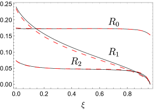
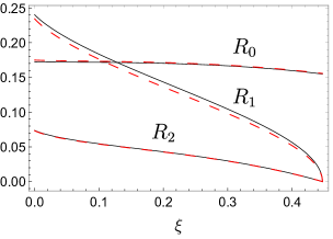
Figure 1: The ratios $R_{k}$ (109) of the imaginary parts of the helicity amplitudes taking into account leading kinematic power corrections (black solid curves) and the complete results (101) to $1/(qq^{\prime})^{2}$ accuracy (red dashed curves) as functions of the skewedness parameter for $Q^{2}=5$ GeV² and $t=-1$ GeV². The left panel: $m=0.14$ GeV; the right panel: $m=1$ GeV.

The calculation is done for $Q^{2}=5$ GeV², $t=-1$ GeV² and two values of the the target mass: $m=0.14$ GeV (pion) with $m=1$ GeV (nucleon), see Appendix E for details. The results are presented on the left and the right panel in Fig. 1, respectively. The leading power contributions to the ratios $R_{k}(\xi)$ are shown by solid black curves and the complete results to the $1/(qq^{\prime})^{2}$ accuracy by red dashes.

One sees that the contribution of subleading power corrections is small for all amplitudes. This is especially so for $R_{0}$ and $R_{2}$ where the difference between solid and dashed curves is within the line thickness. The smallness of the $1/(qq^{\prime})^{2}$ corrections in these two cases is due to strong cancellations between the several relevant contributions in the corresponding expressions in (101). This cancellation apparently persists for a rather large class of the GPD models. Note, however, that the smallness of corrections only holds if the expansion is organized in powers of the scalar product $1/|(qq^{\prime})|\sim 1/(Q^{2}+t)$ instead of $1/Q^{2}$. For the chosen values $Q^{2}=5$ GeV² and $t=-1$ GeV this is a 25% effect.

The power correction to the leading, helicity-conserving amplitude $R_{0}$ depends very weakly on $\xi$ whereas $R_{1}$ and $R_{2}$ vanish at the kinematically maximum allowed value of the skewedness parameter $\xi=\xi_{\mathrm{m}ax}$ (60) owing to the $|P_{\perp}|$ factors in their definition. The value of $\xi_{\mathrm{m}ax}$ depends strongly on the target mass, which explains the difference of the plots on the left (small mass) and right (large mass) panels. At small values of $\xi$ there is practically no difference, since, as already mentioned earlier, the target mass corrections enter through the combination $\xi^{2}m^{2}$ and become irrelevant at large energies.

5 Conclusions

Using the recent results Braun:2020zjm on the contributions of descendants of the leading twist operators to the operator product expansion of two electromagnetic currents in conformal QCD, we have presented a calculation of finite-$t$ and target mass corrections to DVCS on scalar targets to the next-to-leading power accuracy. Our main result of phenomenological relevance is that the next-to-leading corrections are small if the expansion is reorganized in powers of $1/(Q^{2}+t)$ instead of $1/Q^{2}$. The calculation can be extended to higher powers. In particular we find that IR divergences in kinematic corrections cancel to all powers to our present accuracy, in the leading order of perturbation theory. We also argue that target mass corrections in the coherent DVCS from nuclei at large energies are small and do not invalidate the factorization theorem.

A generalization of these results to DVCS on spin-1/2 targets (nucleon) should be straightforward, but more tedious. Also kinematic corrections to double-DVCS (with two virtual photons) can be obtained. A more ambitious project would be to calculate kinematic corrections to the contribution of gluon GPD, that requires going over to next-to-leading order in the strong coupling.

Appendix A Derivation of Eqs. (33), (34)

We start from the identities

$$\left[iP^{\alpha\dot{\alpha}},\partial_{\alpha}\bar{\partial}_{\dot{\alpha}}\partial_{+}^{k}\mathcal{O}^{(0)}_{N}\right] =N^{2}\partial_{+}^{k}\mathcal{O}^{(1)}_{N}+\frac{1}{4}k(2N+k+1)\left[iP^{\alpha\dot{\alpha}},\left[iP_{\alpha\dot{\alpha}},\partial_{+}^{k-1}\mathcal{O}^{(0)}_{N}\right]\right],$$ (110a)

$$\left[iP^{\alpha\dot{\alpha}},\partial_{\alpha}\bar{\partial}_{\dot{\alpha}}\partial_{+}^{k}\mathcal{O}^{(1)}_{N}\right] =(N-1)^{2}\partial_{+}^{k}\mathcal{O}^{(2)}_{N}+\frac{1}{4}k(2N+k-1)\left[iP^{\alpha\dot{\alpha}},\left[iP_{\alpha\dot{\alpha}},\partial_{+}^{k-1}\mathcal{O}^{(1)}_{N}\right]\right],$$ (110b)

where $P$ is the momentum operator and we use the two-component spinor notations as defined in Ref. Braun:2011dg , e.g. $P_{\alpha\dot{\alpha}}=P_{\mu}(\sigma^{\mu})_{\alpha\dot{\alpha}}$, $n_{\alpha\dot{\alpha}}=\lambda_{\alpha}\bar{\lambda}_{\dot{\alpha}}$, $\partial_{\alpha}\equiv\frac{\partial}{\partial\lambda^{\alpha}}$, etc. In the matrix elements one can replace $P\mapsto\Delta$ in (110).

Multiplying both sides of (110a) by $\omega_{Nk}(S_{+}^{(1,1)})^{k}z_{12}^{N-1}$ and summing over $N$ and $k$ one obtains

$$\sum_{N,k}\rho_{N}N^{2}z_{12}^{N-1}\int_{0}^{1}du(u\bar{u})^{N}\mathcal{O}^{(1)}_{N}(nz_{21}^{u})=\left(i\left(\Delta^{\alpha\dot{\alpha}}\partial_{\alpha}\partial_{\dot{\alpha}}\right)+\frac{1}{2}\Delta^{2}S_{+}^{(1,1)}\right)\mathscr{O}_{+}(z_{1},z_{2}),$$ (111)

where $\rho_{N}$ and $\omega_{Nk}$ are defined in (4) and (26), respectively, and $\mathscr{O}_{+}(z_{1},z_{2})$ is the light-ray operator for light-like separations,

$$\mathscr{O}_{+}(z_{1},z_{2})=\mathscr{O}(z_{1},z_{2})|_{x\to n}, \mathscr{O}(z_{1},z_{2})=\Pi(x,\lambda)\mathscr{O}_{+}(z_{1},z_{2})\,.$$ (112)

Here $\Pi(x,\lambda)$ is the leading-twist projector, see Ref. (Braun:2011dg, , Eq.(5.26)). Deriving (111) we take into account that $k(2N+k+1)\omega_{Nk}=\omega_{Nk-1}$ and

$$\omega_{Nk}(S_{+}^{(1,1)})^{k}z_{12}^{N-1}=\rho_{N}\int_{0}^{1}du(u\bar{u})^{N}(z_{21}^{u})^{k}.$$ (113)

Finally, applying the leading-twist projector to the both sides of (111) and taking into account that

$$\Pi(x,\lambda)\frac{\partial}{\partial\lambda^{\alpha}}\frac{\partial}{\partial\bar{\lambda}^{\dot{\alpha}}}\mathscr{O}_{+}(z_{1},z_{2})=\frac{1}{2}\partial_{\alpha\dot{\alpha}}\left(S_{0}^{(1,1)}-1\right)\Pi(x,\lambda)\mathscr{O}_{+}(z_{1},z_{2})$$ (114)

one ends up with the relation in Eq. (33).

To derive (34) we start with (110b), multiply both sides by $N^{2}\omega_{Nk}(S_{+}^{(1,1)})^{k}z_{12}^{N-1}$, and sum over $N$ and $k$. After some algebra one obtains

$$\sum_{N}\rho_{N}N^{2}\int_{0}^{1}\!du\,(u\bar{u})^{N}\left\{(N-1)^{2}\mathcal{O}^{(2)}_{N}(nz_{21}^{u})+\Delta^{2}S_{+}^{(1,1)}\int_{0}^{1}\!dt\,t^{2N+1}\mathcal{O}^{(1)}_{N}(ntz_{21}^{u})\right\}z_{12}^{N}\\ =\left(i\left(\Delta^{\alpha\dot{\alpha}}\partial_{\alpha}\partial_{\dot{\alpha}}\right)+\frac{1}{2}\Delta^{2}S_{+}^{(1,1)}\right)\sum_{N}\rho_{N}N^{2}z_{12}^{N-1}\int_{0}^{1}\!du\,(u\bar{u})^{N}\mathcal{O}^{(1)}_{N}(nz_{21}^{u})\,.$$ (115)

Applying the projector $\Pi(x,\lambda)$ to both sides one gets

$$\sum_{N}\rho_{N}N^{2}\int_{0}^{1}\!du\,(u\bar{u})^{N}\left\{(N-1)^{2}[\mathcal{O}^{(2)}_{N}(xz_{21}^{u})]_{lt}+\Delta^{2}S_{+}^{(1,1)}\int_{0}^{1}\!dt\,t^{2N+1}[\mathcal{O}^{(1)}_{N}(ntz_{21}^{u})]_{lt}\right\}z_{12}^{N}\\ =\left\{\big{(}S_{0}^{(1,1)}-2\big{)}(i\Delta\partial_{x})+\frac{1}{2}\Delta^{2}S_{+}^{(1,1)}\right\}\Pi(x,\lambda)\sum_{N}\rho_{N}N^{2}z_{12}^{N-1}\int_{0}^{1}\!du\,(u\bar{u})^{N}\mathcal{O}^{(1)}_{N}(nz_{21}^{u}).$$ (116)

Note the change from $S_{0}^{(1,1)}-1$ in (114) to $S_{0}^{(1,1)}-2$ in the above equation. It happens because the spin of the operator $\mathcal{O}^{(1)}_{N}$ is $N-1$, see definitions in (2). Finally, replacing the last sum in (116) by (33) one arrives at Eq. (34).

Appendix B Light-ray OPE: terms $\tfrac{x^{\mu}x^{\nu}}{x^{4}}[\mathscr{O}^{(1)}_{N}]_{lt}$

Here we illustrate our techniques on another example, the contributions $\sim\tfrac{x^{\mu}x^{\nu}}{x^{4}}\,[\mathscr{O}^{(1)}_{N}]_{lt}$. There are two such terms: one is explicit in line seven (second to the last) of Eq. (2) and another one arises from the second term in the second line of Eq. (2) when $\mathscr{O}^{(0)}_{N}$ is rewritten using (18) in terms of the leading-twist operators. In the sum one obtains

$$-\frac{x^{\mu}x^{\nu}}{x^{4}}\sum_{N>0,\text{even}}\biggl{[}\frac{\rho_{N}N}{(N+1)}\biggr{]}\int_{0}^{1}\!du\,(u\bar{u})^{N}\biggl{\{}\biggl{[}\frac{1}{N}-\frac{\bar{u}}{N+1}+B(N,\bar{u})\biggr{]}+\frac{\bar{u}-u}{N+1}\biggr{\}}[\mathscr{O}^{(1)}_{N}(ux)]_{lt}$$

$$=-\frac{x^{\mu}x^{\nu}}{x^{4}}\sum_{N>0,\text{even}}\biggl{[}\frac{\rho_{N}N}{(N+1)}\biggr{]}\int_{0}^{1}\!du\,(u\bar{u})^{N}\biggl{\{}\frac{1}{N}-\frac{u}{N+1}+B(N,\bar{u})\biggr{\}}[\mathscr{O}^{(1)}_{N}(ux)]_{lt},$$ (117)

where

$$B(N,\bar{u})=\bar{u}^{-N}\int_{0}^{\bar{u}}\frac{dv}{\bar{v}}v^{N+1}.$$ (118)

In this case it is convenient to write $\mathscr{O}^{(1)}_{N}(ux)$ as a formal Taylor series,

$$\mathscr{O}^{(1)}_{N}(ux)\mapsto\sum_{k}\frac{d_{N}}{k!}u^{k}(i\Delta x)^{k},$$ (119)

which allows one to get rid on an unpleasant integral in $B(N,\bar{u})$. One obtains

$$\int_{0}^{1}\!du\,(u\bar{u})^{N}\biggl{\{}\frac{1}{N}-\frac{u}{N+1}+B(N,\bar{u})\biggr{\}}u^{k}=\frac{\Gamma(N+1)\Gamma(N+k+1)}{\Gamma(2N+k+2)}\biggl{\{}\frac{1}{N(N+1)}+\frac{1}{N+k+1}\biggr{\}},$$ (120)

so that we get

$$-\frac{x^{\mu}x^{\nu}}{x^{4}}\sum_{N,k}\frac{d_{N}}{k!}(i\Delta x)^{k}\rho_{N}N^{2}\frac{\Gamma(N+1)\Gamma(N+k+1)}{\Gamma(2N+k+2)}\biggl{\{}\frac{1}{N^{2}(N+1)^{2}}+\frac{1}{N(N+1)}\frac{1}{N+k+1}\biggr{\}}.$$ (121)

Now we can employ the operator identity (33) where we set $z_{1}=z$, $z_{2}=0$. Using (119) it becomes

$$\sum_{N,k}\frac{d_{N}}{k!}(i\Delta x)^{k}\rho_{N}N^{2}z^{N+k-1}\frac{\Gamma(N+1)\Gamma(N+k+1)}{\Gamma(2N+k+2)}\\ =\Big{(}z\partial_{z}+1\Big{)}(i\Delta\partial_{x})\mathscr{O}(z,0)+\frac{1}{2}\Big{(}z^{2}\partial_{z}+2z\Big{)}\Delta^{2}\mathscr{O}(z,0)\,.$$ (122)

As explained in the text, extra factors $1/(N(N+1))^{k}$ can be emulated by application of the invariant operator $\mathcal{H}_{+}:T^{(1)}\otimes T^{(1)}\mapsto T^{(1)}\otimes T^{(1)}$:

$$[\mathcal{H}_{+}f](z_{1},z_{2}) =\int_{0}^{1}\!d\alpha\!\int_{0}^{\bar{\alpha}}\!d\beta\,f(z_{12}^{\alpha},z_{21}^{\beta})\,,$$

$$[\mathcal{H}^{2}_{+}f](z_{1},z_{2}) =-\int_{0}^{1}\!d\alpha\!\int_{0}^{\bar{\alpha}}\!d\beta\,\ln(\bar{\tau})\,f(z_{12}^{\alpha},z_{21}^{\beta})\,,\qquad\tau=\frac{\alpha\beta}{\bar{\alpha}\bar{\beta}}\,,$$ (123)

The remaining factor $1/(N+k+1)$ can be eliminated by rescaling of the quark-antiquark separation. To see this, replace $z\to tz$ in Eq. (122) and integrate

$$\int_{0}^{1}\!dt\,t\bigg{\{}\Big{(}z\partial_{z}+1\Big{)}(i\Delta\partial_{x})\mathscr{O}(tz,0)+\frac{1}{2}t\Big{(}z^{2}\partial_{z}+2z\Big{)}\Delta^{2}\mathscr{O}(tz,0)\biggr{\}}=$$ (124)

$$= \int_{0}^{1}\!dt\,t\biggl{\{}\sum_{N,k}\frac{d_{N}}{k!}(i\Delta x)^{k}\rho_{N}N^{2}(tz)^{N+k-1}\frac{\Gamma(N+1)\Gamma(N+k+1)}{\Gamma(2N+k+2)}\biggr{\}}$$

$$= \sum_{N,k}\frac{d_{N}}{k!}(i\Delta x)^{k}\rho_{N}N^{2}z^{N+k-1}\frac{\Gamma(N+1)\Gamma(N+k+1)}{\Gamma(2N+k+2)}\frac{1}{N+k+1}\,.$$

Thus we get the contribution of the structure $\tfrac{x^{\mu}x^{\nu}}{x^{4}}[\mathscr{O}^{(1)}_{N}]_{lt}$,

$$\ldots =-\frac{x^{\mu}x^{\nu}}{x^{4}}\bigg{\{}\Big{(}\mathcal{S}-1\Big{)}\mathcal{H}_{+}^{2}(i\Delta\partial_{x})\mathscr{O}(z,0)+\frac{1}{2}\Delta^{2}\mathcal{S}\mathcal{H}_{+}^{2}\mathscr{O}(z,0)\biggr{\}}\biggr{|}_{z=1}$$

$$\quad-\frac{x^{\mu}x^{\nu}}{x^{4}}\int_{0}^{1}\!dt\,t\,\bigg{\{}(i\Delta\partial_{x})[\Big{(}\mathcal{S}-1\Big{)}\mathcal{H}_{+}\mathscr{O}](tz,0)+\frac{1}{2}\Delta^{2}t[\mathcal{S}\mathcal{H}_{+}\mathscr{O}](tz,0)\biggr{\}}\biggr{|}_{z=1},$$ (125)

where $\mathcal{S}:\,T^{(1)}\otimes T^{(1)}\mapsto T^{(\frac{3}{2})}\otimes T^{(\frac{1}{2})}$ is the invariant operator introduced in Eq. (40). Following the argumentation in section 2.2.2, we obtain

$$[\mathcal{S}\mathcal{H}_{+}f](z_{1},z_{2}) =\int_{0}^{1}\!d\beta\,f(z_{1},z_{21}^{\beta})\,,$$

$$[\mathcal{S}\mathcal{H}_{+}^{2}f](z_{1},z_{2}) =\int_{0}^{1}\!d\alpha\!\int_{0}^{\bar{\alpha}}\!d\beta\,\frac{\beta}{\bar{\beta}}f(z_{12}^{\alpha},z_{21}^{\beta})\,,$$ (126)

where from

$$\int_{0}^{1}\!dt\,t\,\Big{[}\mathcal{S}\,\mathcal{H}_{+}f\Big{]}(tz,0) =\int_{0}^{1}\!d\alpha\,\int_{0}^{\bar{\alpha}}\!d\beta f(\bar{\alpha}z,\beta z)\,,$$

$$\int_{0}^{1}\!dt\,t^{2}\,\Big{[}\mathcal{S}\,\mathcal{H}_{+}f\Big{]}(tz,0) =\int_{0}^{1}\!d\alpha\,\bar{\alpha}\!\int_{0}^{\bar{\alpha}}\!d\beta f(\bar{\alpha}z,\beta z)\,,$$

$$\int_{0}^{1}\!dt\,t\,\Big{[}\mathcal{H}_{+}f\Big{]}(tz,0) =-\int_{0}^{1}\!d\alpha\int_{0}^{\bar{\alpha}}\!d\beta\,\ln\bar{\alpha}\,f(\bar{\alpha}z,\beta z)\,.$$ (127)

Collecting everything, we end up with the desired expression

$$-\frac{x^{\mu}x^{\nu}}{x^{4}}\int_{0}^{1}\!d\alpha\int_{0}^{\bar{\alpha}}\!d\beta\biggl{\{}\left(\frac{\beta}{\bar{\beta}}+\ln\bar{\tau}+1+\ln\bar{\alpha}\right)(i\Delta\partial_{x})\mathscr{O}(\bar{\alpha},\beta)+\left(\frac{\beta}{\bar{\beta}}+\bar{\alpha}\right)\frac{1}{2}\Delta^{2}\mathscr{O}(\bar{\alpha},\beta)\biggr{\}}.$$ (128)

Appendix C Leading-twist exponential function

The leading-twist projection of the nonlocal quark-antiquark operator (21) satisfies Laplace equation $\partial_{x}^{2}\mathscr{O}(z_{1},z_{2})=0$ Balitsky:1987bk , see section 2.2, so that the expression on the r.h.s. of (79) must satisfy the same equation. Hence

$$\partial_{x}^{2}\big{[}e^{-i\ell x}\big{]}_{lt}=\partial_{\ell}^{2}\big{[}e^{-i\ell x}\big{]}_{lt}=0\,$$ (129)

with the boundary condition that a usual exponential function is recovered if $x^{2}=0$ or $\ell^{2}=0$. The solution can be written as a power series Balitsky:1987bk

$$[e^{-i\ell x}]_{lt} =e^{-i\ell x}+\sum_{n=1}^{\infty}\int_{0}^{1}\!dt\,(\tfrac{1}{4}x^{2}\ell^{2})^{n}\frac{t^{n}\,\bar{t}^{n-1}}{(n-1)!\,n!}e^{-it\ell x},$$ (130)

where in most applications only the first few terms are needed, cf. (16). Nevertheless, a closed expression summing all powers can be derived Balitsky:1990ck

$$[e^{-i(\ell x)}]_{lt} =e^{-\frac{i}{2}(\ell x)}\left[\cos\left(\frac{1}{2}r(\ell x)\right)-\frac{i}{r}\sin\left(\frac{1}{2}r(\ell x)\right)\right],$$ (131)

where

$$r=\sqrt{1-\frac{\ell^{2}x^{2}}{(x\cdot\ell)^{2}}}\,.$$ (132)

Note that the expansion of (131) only involves even powers of $r$, so that there is no cut at $r=0$.

The Fourier transform of $[e^{-i(\ell x)}]_{lt}$ can be written in closed form as well,

$$i\int\frac{d^{4}x}{\pi^{2}}\,\frac{e^{iq^{\prime}x}[e^{-i\ell x}]_{lt}}{[-x^{2}+i0]^{p}} =\frac{\Gamma(2-p)}{2^{2p-3}\Gamma(p)}\biggl{[}\left(1-\frac{(q^{\prime}\ell)}{s_{2}}\right)(s_{1}-s_{2})^{p-2}+\left(1+\frac{(q^{\prime}\ell)}{s_{2}}\right)(s_{1}+s_{2})^{p-2}\biggr{]},$$ (133)

with

$$s_{1}=(q^{\prime}\ell)-q^{\prime 2}\,, s_{2}=\sqrt{(q^{\prime}\ell)^{2}-\ell^{2}q^{\prime 2}}$$ (134)

Appendix D Helicity amplitudes in the DD representation

In this Appendix we present the expressions for the helicity amplitudes in the DD representation:

$$\mathcal{A}_{0} =\!\iint\!d\alpha d\beta\Phi(\beta,\alpha,t)\Biggl{\{}\!\left(2+\frac{t}{2(qq^{\prime})}\right)\ln(1-F)+\frac{1}{(qq^{\prime})}\left(t\operatorname{Li}_{2}(F)+\beta\left(\frac{t}{\xi}\!-{|P_{\perp}|^{2}}(\beta\partial_{F})\right)T_{3}(F)\right)$$

$$\quad+\frac{t^{2}}{(qq^{\prime})^{2}}\left(\frac{1}{2}\operatorname{Li}_{2}(F)-(1-F)\ln(1-F)\right)+\frac{2t}{(qq^{\prime})^{2}}\beta\left(\frac{t}{\xi}-|P_{\perp}|^{2}(\beta\partial_{F})\right)T_{2}(F)$$

$$\quad+\frac{\beta}{(qq^{\prime})^{2}}\left(-\frac{t^{2}}{2\xi^{2}}+t|P_{\perp}|^{2}\left(1+\frac{1}{\xi}(\beta\partial_{F})\right)-\frac{|P_{\perp}|^{4}}{4}(\beta\partial_{F})^{2}\right)(\beta\partial_{F})T_{5}(F)\Biggr{\}},$$

$$\mathcal{A}_{1} =-\frac{2Q}{(qq^{\prime})}\iint d\alpha d\beta\Phi(\beta,\alpha,t)\,\beta\Biggl{\{}T_{1}(F)+\frac{1}{(qq^{\prime})}\biggl{(}tT_{3}(F)+\left(\frac{t}{\xi}-\frac{|P_{\perp}|^{2}}{2}(\beta\partial_{F})\right)(\beta\partial_{F})T_{2}(F)\biggr{)}\Biggr{\}},$$

$$\mathcal{A}_{2} =\frac{1}{(qq^{\prime})}\iint d\alpha d\beta\Phi(\beta,\alpha,t)\,\beta(\beta\partial_{F})\Biggl{\{}2\left(1+\frac{t}{4(qq^{\prime})}\right)\widetilde{T}_{1}(F)$$

$$\quad-\frac{1}{(qq^{\prime})}\left(3t+\frac{3t}{2\xi}(\beta\partial_{F})-\frac{|P_{\perp}^{2}|}{2}(\beta\partial_{F})^{2}\right)T_{2}(F)\Biggr{\}},$$ (135)

where $F=\tfrac{1}{2}(\tfrac{\beta}{\xi}+\alpha+1)$ (76) and the functions $T_{i}(F)$, $\widetilde{T}_{1}(F)$ are defined in (102).

Appendix E Numerics

The expressions (101) for the amplitudes $\mathcal{A}_{k}$, $k=0,1,2$ contain derivatives with respect to $\xi$ up to the fourth order. There are strong cancellations between the terms with different powers of $D_{\xi}$ in (101). This leads to a loss of accuracy in numerical calculations. In order to avoid this problem it is preferably to bring the expressions for the amplitudes into the form

$$\text{Im}\,\mathcal{A}=\int dx\,F(x,\xi,t),$$ (136)

where the integrand $F$ receive contributions from terms with different powers of $D_{\xi}$. In order to do it we rescale $x\to x\xi$ in (64) and write the convolution of the coefficient function and the GPD (107) in the form:

$$J(\eta) =\int_{1}^{\eta}dxV(x)\int_{\frac{x-1}{\eta-1}}^{\frac{x+1}{\eta+1}}\frac{d\beta}{\beta^{1+a(t)}}\biggl{[}\bar{\beta}^{2}-({x-\beta\eta})^{2}\biggr{]}\,,$$ (137)

where $\eta=1/\xi$ and

$$V(x)=\frac{3}{8}x\,\text{Im}\,T\left(\frac{1+x}{2}\right)\,.$$ (138)

Since $D_{\xi}=-\partial_{\eta}$ we need to evaluate derivatives of $J(\eta)$ with respect to $\eta$. Taking the derivative of (137) one find that all boundary terms vanish and the final expression takes the form:

$$\partial_{\eta}J(\eta)=2\int_{1}^{\eta}dxV(x)\int_{\frac{x-1}{\eta-1}}^{\frac{x+1}{\eta+1}}\frac{d\beta}{\beta^{a(t)}}(x-\beta\eta)=2\int_{1}^{\eta}dxV(x)\left(xT_{a}(x,\eta)-\eta T_{a-1}(x,\eta)\right)\,,$$ (139)

where

$$T_{a}(x,\eta) =\int_{\frac{x-1}{\eta-1}}^{\frac{x+1}{\eta+1}}\frac{d\beta}{\beta^{a(t)}}=\frac{1}{1-a}\left(\left(\frac{x+1}{\eta+1}\right)^{1-a}-\left(\frac{x-1}{\eta-1}\right)^{1-a}\right)\,.$$ (140)

Similarly, one finds

$$\partial_{\eta}^{k}J(\eta)=2\int_{1}^{\eta}dxV(x)\partial_{\eta}^{k-1}\left(xT_{a}(x,\eta)-\eta T_{a-1}(x,\eta)\right)+\delta_{k4}\frac{8V(\eta)}{(\eta^{2}-1)^{2}}\,,$$ (141)

for $k=1,2,3,4$. It allows one to write the amplitudes in the form (136) and avoid the problem with accuracy.

References

- (1) R. Abdul Khalek et al., Science Requirements and Detector Concepts for the Electron-Ion Collider: EIC Yellow Report, 2103.05419.
- (2) R. Abdul Khalek et al., Snowmass 2021 White Paper: Electron Ion Collider for High Energy Physics, in 2022 Snowmass Summer Study, 3, 2022. 2203.13199.
- (3) D. Müller, D. Robaschik, B. Geyer, F. M. Dittes and J. Hořejši, Wave functions, evolution equations and evolution kernels from light ray operators of QCD, Fortsch. Phys. 42 (1994) 101–141, [hep-ph/9812448].
- (4) X.-D. Ji, Deeply virtual Compton scattering, Phys. Rev. D 55 (1997) 7114–7125, [hep-ph/9609381].
- (5) A. V. Radyushkin, Nonforward parton distributions, Phys. Rev. D 56 (1997) 5524–5557, [hep-ph/9704207].
- (6) X.-D. Ji and J. Osborne, One loop corrections and all order factorization in deeply virtual Compton scattering, Phys. Rev. D 58 (1998) 094018, [hep-ph/9801260].
- (7) A. V. Belitsky, A. Freund and D. Müller, Evolution kernels of skewed parton distributions: Method and two loop results, Nucl. Phys. B 574 (2000) 347–406, [hep-ph/9912379].
- (8) A. V. Belitsky and D. Müller, Broken conformal invariance and spectrum of anomalous dimensions in QCD, Nucl. Phys. B 537 (1999) 397–442, [hep-ph/9804379].
- (9) J. D. Noritzsch, Heavy quarks in deeply virtual Compton scattering, Phys. Rev. D 69 (2004) 094016, [hep-ph/0312137].
- (10) K. Kumericki, D. Müller, K. Passek-Kumericki and A. Schäfer, Deeply virtual Compton scattering beyond next-to-leading order: the flavor singlet case, Phys. Lett. B 648 (2007) 186–194, [hep-ph/0605237].
- (11) K. Kumericki, D. Müller and K. Passek-Kumericki, Towards a fitting procedure for deeply virtual Compton scattering at next-to-leading order and beyond, Nucl. Phys. B 794 (2008) 244–323, [hep-ph/0703179].
- (12) V. M. Braun, A. N. Manashov, S. Moch and M. Strohmaier, Three-loop evolution equation for flavor-nonsinglet operators in off-forward kinematics, JHEP 06 (2017) 037, [1703.09532].
- (13) V. M. Braun, A. N. Manashov, S. Moch and J. Schoenleber, Two-loop coefficient function for DVCS: vector contributions, JHEP 09 (2020) 117, [2007.06348].
- (14) V. M. Braun, A. N. Manashov, S. Moch and J. Schoenleber, Axial-vector contributions in two-photon reactions: Pion transition form factor and deeply-virtual Compton scattering at NNLO in QCD, Phys. Rev. D 104 (2021) 094007, [2106.01437].
- (15) J. Gao, T. Huber, Y. Ji and Y.-M. Wang, Next-to-Next-to-Leading-Order QCD Prediction for the Photon-Pion Form Factor, Phys. Rev. Lett. 128 (2022) 062003, [2106.01390].
- (16) V. M. Braun, K. G. Chetyrkin and A. N. Manashov, NNLO anomalous dimension matrix for twist-two flavor-singlet operators, Phys. Lett. B 834 (2022) 137409, [2205.08228].
- (17) S. Van Thurenhout and S. Moch, Off-forward anomalous dimensions in the leading- limit, 6, 2022. 2206.04517.
- (18) V. M. Braun, Y. Ji and J. Schoenleber, Deeply Virtual Compton Scattering at Next-to-Next-to-Leading Order, Phys. Rev. Lett. 129 (2022) 172001, [2207.06818].
- (19) CLAS collaboration, M. Hattawy et al., First Exclusive Measurement of Deeply Virtual Compton Scattering off 4He: Toward the 3D Tomography of Nuclei, Phys. Rev. Lett. 119 (2017) 202004, [1707.03361].
- (20) CLAS collaboration, R. Dupré et al., Measurement of deeply virtual Compton scattering off with the CEBAF Large Acceptance Spectrometer at Jefferson Lab, Phys. Rev. C 104 (2021) 025203, [2102.07419].
- (21) V. M. Braun, A. N. Manashov, D. Müller and B. Pirnay, Resolving kinematic ambiguities in QCD predictions for Deeply Virtual Compton Scattering, PoS DIS2014 (2014) 225, [1407.0815].
- (22) V. M. Braun, A. N. Manashov, D. Müller and B. M. Pirnay, Deeply Virtual Compton Scattering to the twist-four accuracy: Impact of finite- and target mass corrections, Phys. Rev. D 89 (2014) 074022, [1401.7621].
- (23) Y. Guo, X. Ji and K. Shiells, Higher-order kinematical effects in deeply virtual Compton scattering, JHEP 12 (2021) 103, [2109.10373].
- (24) Jefferson Lab Hall A collaboration, M. Defurne et al., E00-110 experiment at Jefferson Lab Hall A: Deeply virtual Compton scattering off the proton at 6 GeV, Phys. Rev. C 92 (2015) 055202, [1504.05453].
- (25) M. Defurne et al., A glimpse of gluons through deeply virtual compton scattering on the proton, Nature Commun. 8 (2017) 1408, [1703.09442].
- (26) V. Braun, A. Manashov and B. Pirnay, Finite-t and target mass corrections to DVCS on a scalar target, Phys. Rev. D 86 (2012) 014003, [1205.3332].
- (27) Jefferson Lab Hall A collaboration, F. Georges et al., Deeply virtual Compton scattering cross section at high Bjorken , 2201.03714.
- (28) V. Braun and A. Manashov, Kinematic power corrections in off-forward hard reactions, Phys. Rev. Lett. 107 (2011) 202001, [1108.2394].
- (29) V. Braun and A. Manashov, Operator product expansion in QCD in off-forward kinematics: Separation of kinematic and dynamical contributions, JHEP 01 (2012) 085, [1111.6765].
- (30) V. Braun, A. Manashov and B. Pirnay, Finite-t and target mass corrections to deeply virtual Compton scattering, Phys. Rev. Lett. 109 (2012) 242001, [1209.2559].
- (31) V. M. Braun, Y. Ji and A. N. Manashov, Two-photon processes in conformal QCD: Resummation of the descendants of leading-twist operators, JHEP 51 (2021) 51, [2011.04533].
- (32) S. Ferrara, A. Grillo and R. Gatto, Manifestly conformal covariant operator-product expansion, Lett. Nuovo Cim. 2S2 (1971) 1363–1369.
- (33) S. Ferrara, R. Gatto and A. Grillo, Conformal invariance on the light cone and canonical dimensions, Nucl. Phys. B 34 (1971) 349–366.
- (34) S. Ferrara, A. Grillo and R. Gatto, Tensor representations of conformal algebra and conformally covariant operator product expansion, Annals Phys. 76 (1973) 161–188.
- (35) K. Wilson and J. B. Kogut, The Renormalization group and the epsilon expansion, Phys. Rept. 12 (1974) 75–199.
- (36) V. Braun, A. Manashov, S. Moch and M. Strohmaier, Conformal symmetry of QCD in -dimensions, Phys. Lett. B 793 (2019) 78–84, [1810.04993].
- (37) C. Lorcé, B. Pire and Q.-T. Song, Kinematical higher-twist corrections in , 2209.11140.
- (38) I. I. Balitsky and V. M. Braun, Evolution Equations for QCD String Operators, Nucl. Phys. B 311 (1989) 541–584.
- (39) I. I. Balitsky and V. M. Braun, The Nonlocal operator expansion for inclusive particle production in e+ e- annihilation, Nucl. Phys. B 361 (1991) 93–140.
- (40) V. M. Braun, G. P. Korchemsky and D. Müller, The Uses of conformal symmetry in QCD, Prog. Part. Nucl. Phys. 51 (2003) 311–398, [hep-ph/0306057].
- (41) I. M. Gel’fand, M. I. Graev and N. Y. Vilenkin, Generalized functions. Vol. 5. AMS Chelsea Publishing, Providence, RI, 2016.
- (42) V. Braun, A. Manashov and J. Rohrwild, Renormalization of Twist-Four Operators in QCD, Nucl. Phys. B 826 (2010) 235–293, [0908.1684].
- (43) Y. L. Dokshitzer, G. Marchesini and G. P. Salam, Revisiting parton evolution and the large-x limit, Phys. Lett. B 634 (2006) 504–507, [hep-ph/0511302].
- (44) B. Basso and G. P. Korchemsky, Anomalous dimensions of high-spin operators beyond the leading order, Nucl. Phys. B 775 (2007) 1–30, [hep-th/0612247].
- (45) L. F. Alday, A. Bissi and T. Lukowski, Large spin systematics in CFT, JHEP 11 (2015) 101, [1502.07707].
- (46) L. F. Alday and A. Zhiboedov, An Algebraic Approach to the Analytic Bootstrap, JHEP 04 (2017) 157, [1510.08091].
- (47) A. V. Belitsky, D. Müller and Y. Ji, Compton scattering: from deeply virtual to quasi-real, Nucl. Phys. B 878 (2014) 214–268, [1212.6674].
- (48) A. V. Radyushkin, Symmetries and structure of skewed and double distributions, Phys. Lett. B 449 (1999) 81–88, [hep-ph/9810466].
- (49) O. V. Teryaev, Crossing and radon tomography for generalized parton distributions, Phys. Lett. B 510 (2001) 125–132, [hep-ph/0102303].
- (50) A. V. Belitsky and D. Müller, Exclusive electroproduction revisited: treating kinematical effects, Phys. Rev. D 82 (2010) 074010, [1005.5209].
- (51) A. V. Radyushkin, Generalized Parton Distributions and Their Singularities, Phys. Rev. D 83 (2011) 076006, [1101.2165].
- (52) S. V. Goloskokov and P. Kroll, The Longitudinal cross-section of vector meson electroproduction, Eur. Phys. J. C 50 (2007) 829–842, [hep-ph/0611290].