Electron dynamics in planar radio frequency magnetron plasmas:
I. The mechanism of Hall heating and the $\boldsymbol{\mu}$-mode

The electron dynamics and the mechanisms of power absorption in radio-frequency (RF) driven, magnetically enhanced capacitively coupled plasmas (MECCPs) at low pressure are investigated. The device in focus is a geometrically asymmetric cylindrical magnetron with a radially nonuniform magnetic field in axial direction and an electric field in radial direction. The dynamics is studied analytically using the cold plasma model and a single-particle formalism, and numerically with the inhouse energy and charge conserving particle-in-cell/Monte Carlo collisions code ECCOPIC1S-M. It is found that the dynamics differs significantly from that of an unmagnetized reference discharge. In the magnetized region in front of the powered electrode, an enhanced electric field arises during sheath expansion and a reversed electric field during sheath collapse. Both fields are needed to ensure discharge sustaining electron transport against the confining effect of the magnetic field. The corresponding azimuthal $\mathbf{E}\!\times\!\mathbf{B}$-drift can accelerate electrons into the inelastic energy range which gives rise to a new mechanism of RF power dissipation. It is related to the Hall current and is different in nature from Ohmic heating, as which it has been classified in previous literature. The new heating is expected to be dominant in many magnetized capacitively coupled discharges. It is proposed to term it the “$\mu$-mode” to separate it from other heating modes.

I Introduction

An externally applied magnetic field allows to sustain gas discharges at lower pressures and at higher plasma densities than otherwise possible lieberman_2005 . Magnetically enhanced plasmas play a major role in advanced surface processing technologies such as thin film deposition, plasma etching, or ion implantation thornton_1978 ; chapman_1980 ; LinHinsonClassSandstrom1984 ; depla_2008 ; manos_1989 . They are often termed “partially” or “weakly” magnetized, referring to the fact that – at typical magnetic flux densities $B$ of up to $100\,\mathrm{mT}$ – only electrons are magnetized, while ions are not. (A particle is called magnetized when its gyration radius $r_{\mathrm{L}}$ is smaller than other length scales like the reactor size $L$, the scale length of the magnetic field $l$, and the mean free path $\lambda$, and its gyration frequency $\omega_{\mathrm{c}}$ larger that than other relevant frequencies like the modulation frequency $\omega_{\mathrm{RF}}$ or the collision frequency $\nu$ HagelaarOudini2011 .) In this study, we focus on radio-frequency (RF) driven magnetrons thornton_1981 ; Piel2017 , or, more generally, on magnetically enhanced capacitively coupled plasmas (MECCPs), where a radio-frequency voltage drives an electrical current across the magnetic field kushner_2003 .

In order to optimize and control such discharges, it is crucial to understand how exactly magnetized electrons acquire and utilize their power. The aspect of “utilization” is obvious: Magnetization can confine energetic electrons to an active region which they can leave only by collisional interaction (classical transport) or by scattering at instability-induced fluctuations of the electric field (anomalous transport). This improves utilization of the electron energy. In some discharge configurations such as planar magnetrons, the electron drift orbits are closed within the reactor, so that the effective system size becomes infinite Rossnagel2020 .

The processes which enable the electrons to acquire energy are more difficult to address. In a fluid view, electron heating, as the phenomenon is called, requires an electron current $\boldsymbol{j}_{\mathrm{e}}$in the direction of the electric field $\boldsymbol{E}$: The power dissipation, i.e., the energy flow from the electromagnetic field to the electrons, is equal to $P_{\mathrm{e}}=\boldsymbol{j}_{\mathrm{e}}\!\cdot\!\boldsymbol{E}$. The mechanisms underlying the transport of electrons in magnetized plasmas are diverse and notoriously complicated BoeufSmolyakov2018 ; Kaganovichetal2020 .Equally complicated are the mechanisms of electron heating in MECCPs. Note that the fluid picture itself may be physically insufficient and should be supplemented by kinetic analysis: Only those electrons whose kinetic energies are above the inelastic thresholds of chemical reactions can create useful new particles and radiation. Low-energy electrons do not have this chance and merely take part in transport processes. This consideration would motivate to distinguish between electron heating in general and electron energization in particular anders_2014 .

To get oriented, it helps to first consider the power absorption in non-magnetized CCPs. Traditionally, Ohmic heating was assumed: The electrical field parallel to the electron flux was taken to arise from Ohmic resistance, i.e., from the need to overcome electron inertia and the momentum loss connected to elastic collisions with the neutral background particles lieberman_2005 . This process can already be captured within the Drude model. (We use standard notation:$m_{\mathrm{e}}$ is the electron mass, $e$ the electron charge, $n_{\mathrm{e}}$ the electron density, $\omega_{\mathrm{RF}}$ the frequency of the applied voltage, and $\nu_{\mathrm{e}}=v_{\mathrm{the}}/\lambda_{\mathrm{e}}$ the electron neutral collision frequency, where $\lambda_{\mathrm{e}}$ is the mean free path and $v_{\mathrm{the}}=\sqrt{8T_{\mathrm{e}}/\pi m_{\mathrm{e}}}$ the thermal speed; $T_{\mathrm{e}}$ is the electron temperature.) In the frequency domain, the plasma conductivity is the complex $\underline{\sigma}_{\mathrm{e}}=e^{2}n_{\mathrm{e}}/(i\omega_{\mathrm{RF}}+\nu_{\mathrm{e}})m_{\mathrm{e}}$. The electron current is $\underline{\boldsymbol{j}}_{\mathrm{e}}=\underline{\sigma}_{\mathrm{e}}\underline{\boldsymbol{E}}$, and the phase-averaged dissipated power, understood to be converted into electron thermal energy, reads:

$$\bar{P}_{\Omega}=\frac{1}{4}\left(\underline{\boldsymbol{j}}_{\mathrm{e}}\!\cdot\!\underline{\boldsymbol{E}}^{*}+\underline{\boldsymbol{j}}_{\mathrm{e}}^{*}\!\cdot\!\underline{\boldsymbol{E}}\right)=\frac{e^{2}n_{\mathrm{e}}\nu_{\mathrm{e}}}{2m_{\mathrm{e}}\left(\nu_{\mathrm{e}}^{2}+\omega_{\mathrm{RF}}^{2}\right)}\,\underline{\boldsymbol{E}}\!\cdot\!\underline{\boldsymbol{E}}^{*}.$$ (1)

Kinetic theory gives insight into the underlying mechanism. Assuming that the electric field is not too strong – $e\lambda_{\mathrm{e}}|\boldsymbol{E}|\ll T_{\mathrm{e}}$, so that the energy increment between collisions is small –, Ohmic heating is a diffusion process in energy space. The corresponding diffusion constant is proportional to the square of the effective electric field and, provided that the elastic collision frequency is smaller than the radio frequency, proportional to the pressure $p$ tsendin_2011 ; kudryavtsev_2010 .At low gas pressure, however, the concept of Ohmic heating loses its explanatory power.An alternative mechanism, termed “stochastic heating”, was proposed by Godyak Godyak1972 ; LiebermanGodyak1998 . The modulated plasma sheath, specifically the electron edge, was treated as an oscillating, specularly reflecting “hard wall”. As a consequence, if an electron of velocity $v$ collides with the edge moving at speed $u_{\mathrm{s}}$, then the electron velocity after the collision is $2u_{\mathrm{s}}-v$. Under the assumption that the oscillation of the electron edge and the trajectories of the individual electrons are not correlated – which explains the term ”stochastic heating” –, this process leads, on average, to an increase in kinetic energy. (It is evident that the stated assumption is problematic, and recent treatments seek to avoid it. However, the name stuck.)Further investigations have shown that, for typical plasma conditions, stochastic heating cannot really be of a collision-free nature. Rather, it must be of a ”hybrid” type in that it requires an additional dissipative mechanism in the plasma bulk, for example elastic electron-neutral collisions, even if these are only implicitely accounted for Kaganovich1996 ; Lafleur2015 .

It was also found that not only the moving sheath edge, but also the momentarily quasineutral zone behind it contributes to the power dissipation via the ambipolar field GozadinosTurnerVender2001 ; SchulzeDonkoDerzsiKorolovSchuengel2015 . The concept of “pressure heating” is based on the assumption that sheath heating is caused by the periodic but temporally asymmetric compression and decompression of the electron fluid near the sheath GozadinosTurnerVender2001 ; Turner2009 . Reference Lafleur2014 argued that stochastic heating and pressure heating stem from the same physical mechanism; they differ only in the spatial region where the electron heating is assumed to occur. For a finite net power absorption, the sheath expansion must not be a “mirror image” of the collapse, so that the dissipation integral $\oint\boldsymbol{j}_{\mathrm{e}}\!\cdot\!\mathrm{d}\boldsymbol{E}$ is unequal to zero Turner2009 ; SchulzeDonkoLafleurWilczekBrinkmann2018 .

Additional electron heating mechanisms which can be linked to sheath physics are caused by the action of a reversed electric field during sheath collapse (“field reversal heating”) sato_1990 ; vender_1992 ; tochikubo_1992 ; schulze_2008 ; eremin_2015 and the self-excitation of the plasma series resonance (PSR) through sheath-related nonlinearities in asymmetric discharges (“nonlinear electron resonance heating” NERH) czarnetzki_2006 ; mussenbrock_2008 ; lieberman_2008 ; donko_2009 ; wilczek_2016 ; wilczek_2018 .Lastly, it was found that also secondary electrons, predominantly of the ion-induced $\gamma$-type, can significantly contribute to the electron heating process and even enable a transition of the discharge into the $\gamma$-mode belenguer_1990 ; godyak_1992 . Of course, all listed processes are simultaneously present and may act in synergy Brinkmann2015 .

The literature on the subject shows that all heating mechanisms present in unmagnetized capacitive plasmas can also be seen in their magnetized counterparts, albeit in modified form. An early study by Lieberman, Lichtenberg, and Savas stated that both Ohmic and stochastic heating would be enhanced by a magnetic field, but via different physical mechanisms LiebermanLichtenbergSavas1991 . The increased Ohmic heating was related to a magnetically modified conductivity tensor. Stochastic heating would increase because magnetized electrons can collide multiple times with the sheath during an expansion phase, at each collision picking up additional energy. Both heating processes were argued to scale positively with the magnetic field strength,so that their ratio was predicted to stay constant. Another early study found increased levels of sheath heating under the resonance condition $\omega=2\,\omega_{\mathrm{ce}}$ OkunoOhtsuFujita1994 . This effect, which requires unusually small magnetic fields, was revisited in Zhang2021 and Patil2022 , where it acquired a new name “electron bounce-cyclotron resonance heating”. Later research came to different results. Using experiments, particle-in-cell/Monte Carlo collisions simulations, or analytical models, references HutchinsonTurnerDoyleHopkins1995 ; TurnerHutchinsonDoyleHopkins1996 ; KrimkeUrbassek1995 claimed that even weak magnetic fields could make Ohmic heating prevail over other heating mechanisms. More recent work has argued similarly BarnatMillerPaterson2008 ; YouHaiParkKimKimSeongShinLeeParkLeeChang2011 ; ZhengWangGrotjohnSchuelkeFan2019 .

Also the other mechanisms were seen in magnetized plasmas. NERH was investigated for different values of the magnetic flux density in RF driven planar magnetron plasmas oberberg_2019 ; joshi_2018 . Electric field reversal was also observed and connected with the inhibited electron transport due to the magnetic field yeom_1989 ; krimke_1994 ; kushner_2003 ; WangWenHartmannDonkoDerzsiWangSongWangSchulze2020 . Influence of ambipolar field heating was seen in WangWenHartmannDonkoDerzsiWangSongWangSchulze2020 . Also secondary electron emission can play a role. Kushner concluded that if the magnetic field is oriented parallel to the electrode, heating by secondary electrons (of the $\gamma$-type) is most effective when their gyroradius is comparable to the elastic mean free path kushner_2003 .Other research, however, indicated that a presence of secondaries is not always important for discharge sustainment zheng_2021 .

As stated above, all electron heating mechanisms present in unmagnetized capacitive plasmas are also active in MECCPs, albeit in modified form. But does this also apply vice versa? Can all electron heating processes in MECCPs be understood in terms of their counterparts in unmagnetized CCPs? We do not believe this is the case. Instead, we believe that the dominant heating in MECCPs is ”truly magnetic” but has not been recognized as such. In particular, we believe that the term “Hall-enhanced Ohmic heating” ZhengWangGrotjohnSchuelkeFan2019 is a misnomer, and that the underlying phenomenon has little in common with the process of Ohmic heating, provided that term is used in the original sense. We propose to call it “Hall heating” or, with reference to the role of the magnetic field, the $\mu$-mode. In this study we will outline our arguments and support them with analysis and simulation. Specifically, we will contrast the characteristics of a magnetized discharge with a nominal field strength of $B=5\,\mathrm{mT}$ with an unmagnetized reference case of the same geometry. (If necessary, we mark the magnetized and unmagnetized case with (M) and (U), respectively.)

This publication is the first of three companion papers aimed at improving the understanding of the electron dynamics in magnetized radio frequency discharges operated at low pressures. It emphasizes the kinetic nature of the electron heating in such discharges and demonstrates that the dominant Hall heating is a new mechanism that directly leads to efficient ionization. To focus on the electron transport across the magnetic field lines, we study a long cylindrical magnetron in axisymmetric approximation. The second work eremin_2021 computationally studies a planar RF magnetron in realistic geometry with electron motion along the magnetic field.

Finally, the third publication berger_2021 presents experimental observations obtained in a planar RF magnetron and interprets them with help of the newly gained knowledge about the electron dynamics in such devices.

II The device under study and its operation regime

Our research focuses on a cylindrical magnetron with pronounced geometrical asymmetry. Fig. 1 provides a schematic and defines the reference directions of the currents and voltages. The powered inner electrode $\mathrm{E}$ has a radius of $R_{\mathrm{E}}=1\,\mathrm{cm}$, the grounded outer electrode $\mathrm{G}$a radius of $R_{\mathrm{G}}=6.5\,\mathrm{cm}$, with $R_{\mathrm{C}}=(R_{\mathrm{E}}+R_{\mathrm{G}})/2$. The electrode area ratio is $A_{\mathrm{E}}/A_{\mathrm{G}}=0.154$. Invariance in the axial and azimuthal directions is assumed. The first assumption makes the discharge infinitely long. (For evaluation purposes, we use a nominal height of $H=10\,\mathrm{cm}$.) The second assumption reflects that symmetry breaking plasma instabilities are generally not significant for the rather weak magnetic fields ($B\leq 10$ mT) considered in this study panjan_2019 ; lucken_2020 ; Xu_2021 . In the radial direction the magnetic field and the plasma characteristics are nonuniform.The device is operated in argon at a pressure of $p=0.5\,\mathrm{Pa}$ and a temperature of $T=300\,\mathrm{K}$. A sinusoidal RF voltage with an amplitude of $\hat{V}=300\,\mathrm{V}$ and a frequency of $f=13.56\,\mathrm{MHz}$ is connected via a large blocking capacitor, over which a self bias of $\bar{V}_{\mathrm{G}}=-161\,\mathrm{V}$ drops. The sheath before the powered electrode has a phase-averaged thickness of $\bar{s}_{\mathrm{E}}\approx 0.32\,\mathrm{cm}$; it develops a large voltage $\bar{V}_{\mathrm{E}}=200\,\mathrm{V}$ that accelerates the impacting ions to high energies. This, in turn, yields a high flux of secondary electrons which are also energized in the sheath. Analogous processes at electrode $\mathrm{G}$ are less effective, there $\bar{s}_{\mathrm{G}}\approx 0.14\,\mathrm{cm}$ and $\bar{V}_{\mathrm{G}}=20\,\mathrm{V}$. The magnetic field $\boldsymbol{B}=B_{z}(r)\boldsymbol{e}_{z}$ is a 1d model of a planar magnetron field oberberg_2019 ; oberberg_2018 ; oberberg_2020 ; berger_2021 . (Clearly, the model field is not curl-free. However, the validity of our analysis is not affected.) Following the logic of reference trieschmann_2013 , we adopt the axial profile of the radial magnetic fieldcomponent directly above the racetrack from eremin_2021 , see Fig. 1. An analytical form is as follows, where $B_{i}=\{-1.46,21.98,-0.90,9.92\}\,{\rm mT}$ and $\lambda_{i}=\{35.4,81.2,127.3,173.4\}\,\mathrm{m}^{-1}$:

$$B_{z}(r)=\sum\limits_{i=1}^{4}B_{i}\exp(-\lambda_{i}r).$$ (2)

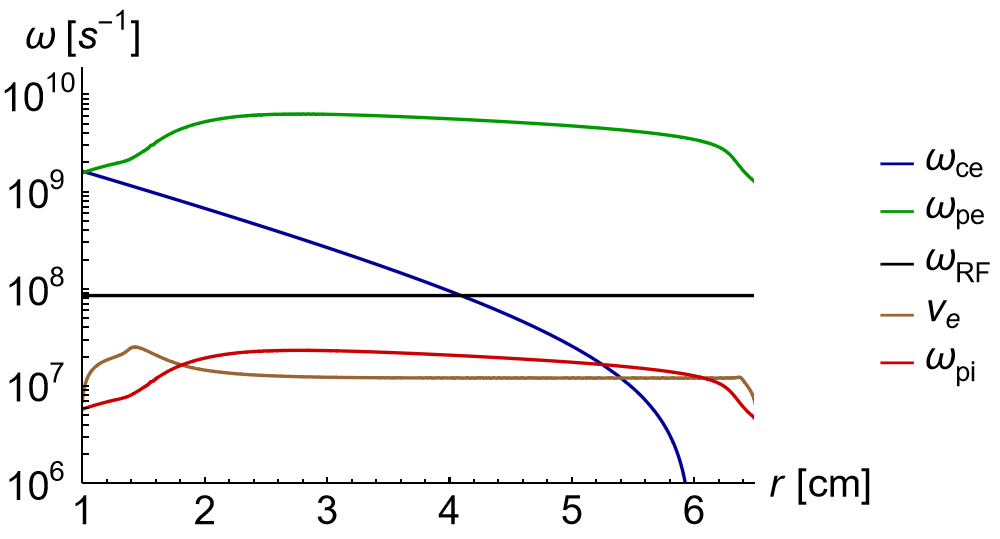
Figure 2: Characteristic frequencies of the cylindrical magnetron, evaluated for the magnetized case. Blue: electron gyrofrequency $\omega_{\mathrm{ce}}$, green: electron plasma frequency $\omega_{\mathrm{pe}}$, black: radio frequency $\omega_{\mathrm{RF}}$,brown: electron collision frequency $\nu_{\mathrm{e}}$, red: ion plasma frequency $\omega_{\mathrm{pi}}$.

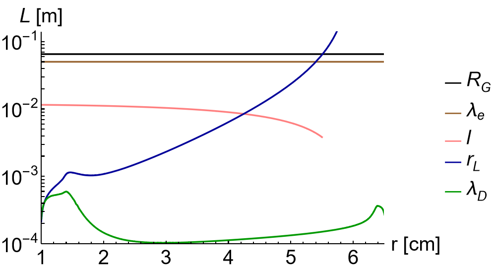
Figure 3: Characteristic length scales of the cylindrical magnetron, evaluated for the magnetized case. Blue: electron gyroradius $r_{\mathrm{L}}$, black: chamber radius $R_{\mathrm{G}}$, pink: field gradient scale $l=|B_{z}/\partial B_{z}/\partial r|$, brown: electron mean free path $\lambda_{\mathrm{e}}$, green: Debye length $\lambda_{\mathrm{D}}$.

Figs. 2 and 3 show the frequency and length scales of the discharge. In the magnetized region, the electron gyro frequency and the plasma frequency are comparable, $\omega_{\mathrm{ce}}\approx\omega_{\mathrm{pe}}\approx 10^{9}\,\mathrm{s}^{-1}$, while the radio frequency and the collision rate are smaller, $\omega_{\mathrm{RF}}\approx 10^{8}\,\mathrm{s}^{-1}$ and $\nu_{\mathrm{e}}\approx 10^{7}\,\mathrm{s}^{-1}$. Likewise, the gyroradius and the Debye length are the smallest scales, $r_{\mathrm{L}}\approx\lambda_{\mathrm{D}}\approx 5\!\times\!10^{-4}\,\mathrm{m}$, the gradient scale is larger, $l\approx 5\!\times\!10^{-3}\,\mathrm{m}$; and the mean free path even more, $\lambda_{\mathrm{e}}\approx 5\!\times\!10^{-2}\,\mathrm{m}$. The electron thermal speed and the $E\!\times\!B$ drift speed are similar, $v_{\mathrm{the}}\approx v_{E\times B}\approx 10^{6}\,\mathrm{m/s}$. The ions are not affected by the magnetic field. (Data from the simulations below.)

III Analysis based on the cold plasma model

A first insight into the discharge dynamics is obtained by considering the cold plasma model, also known as the Drude model lieberman_2005 . We adopt the cylindrical geometry as discussed above. The electron plasma frequency $\omega_{\mathrm{pe}}(r)$ and the electron gyro frequency $\omega_{\mathrm{ce}}(r)$ depend on $r$;the elastic electron collision frequency $\nu_{\mathrm{e}}$ is constant. The equations of continuity and motion for the charge density $\rho(r,t)$ and for the non-vanishing components $j_{r}(r,t)$ and $j_{\theta}(r,t)$ of the electric current density are

$$\frac{\partial\rho}{\partial t}+\frac{1}{r}\frac{\partial}{\partial r}\left(rj_{r}\right)=0,$$ (3)

$$\frac{\partial j_{r}}{\partial t}=\varepsilon_{0}\omega_{\mathrm{pe}}^{2}E_{r}-\omega_{\mathrm{ce}}j_{\theta}-\nu_{\mathrm{e}}j_{r},$$ (4)

$$\frac{\partial j_{\theta}}{\partial t}=\omega_{\mathrm{ce}}j_{r}-\nu_{\mathrm{e}}j_{\theta}.$$ (5)

The electric field $\boldsymbol{E}=E_{r}(r,t)\boldsymbol{e}_{r}$, derived from a potential $\Phi(r,t)$, follows Poisson’s equation

$$\varepsilon_{0}\frac{1}{r}\frac{\partial}{\partial r}\left(rE_{r}\right)=-\varepsilon_{0}\frac{1}{r}\frac{\partial}{\partial r}\left(r\frac{\partial\Phi}{\partial r}\right)=\rho.$$ (6)

As a consequence of the equations, the sum of the particle current and the displacement current is divergence-free. This allows to define the current through the discharge as

$$I(t)=2\pi rH\left(j_{r}+\varepsilon_{0}\frac{\partial E_{r}}{\partial t}\right).$$ (7)

If the time-evolution is harmonic with frequency $\omega$ (which is in this context not necessarily the applied radio frequency $\omega_{\mathrm{RF}}$), the complex currents $\underline{j}_{r}$ and $\underline{j}_{\theta}$ can be expressed as follows.The expressions after the tilde hold in the limiting case $\nu=0$, $\omega\ll\omega_{\mathrm{ce}}$:

$$\underline{j}_{r}=-\frac{(i\omega+\nu_{\mathrm{e}})\varepsilon_{0}\omega_{\mathrm{pe}}^{2}}{\omega^{2}-\omega_{\mathrm{ce}}^{2}-\nu_{\mathrm{e}}^{2}-2i\nu_{\mathrm{e}}\omega}\underline{E}_{r}\sim\frac{i\omega\varepsilon_{0}\omega_{\mathrm{pe}}^{2}}{\omega_{\mathrm{ce}}^{2}}\underline{E}_{r}=en_{\mathrm{e}}\frac{i\omega\underline{E}_{r}}{\omega_{\mathrm{ce}}B_{z}},$$ (8)

$$\underline{j}_{\theta}=-\frac{\omega_{\mathrm{ce}}\varepsilon_{0}\omega_{\mathrm{pe}}^{2}}{\omega^{2}-\omega_{\mathrm{ce}}^{2}-\nu_{\mathrm{e}}^{2}-2i\nu_{\mathrm{e}}\omega}\underline{E}_{r}\sim\frac{\varepsilon_{0}\omega_{\mathrm{pe}}^{2}}{\omega_{\mathrm{ce}}}\underline{E}_{r}=en_{\mathrm{e}}\frac{\underline{E}_{r}}{B_{z}}.$$ (9)

The relation of the discharge current to the electric field can be written as

$$\underline{I}=2\pi rH\,i\omega\varepsilon_{0}\varepsilon_{\mathrm{p}}\underline{E}_{r},$$ (10)

where the relative dielectric constant of the plasma is

$$\varepsilon_{\mathrm{p}}=1-\frac{\omega_{\mathrm{pe}}^{2}(\omega-i\nu_{\mathrm{e}})}{\omega\left(\omega^{2}-\omega_{\mathrm{ce}}^{2}-\nu_{\mathrm{e}}^{2}-2i\nu_{\mathrm{e}}\omega\right)}\approx-\frac{\omega_{\mathrm{pe}}^{2}(\omega-i\nu_{\mathrm{e}})}{\omega\left(\omega^{2}-\omega_{\mathrm{ce}}^{2}-\nu_{\mathrm{e}}^{2}-2i\nu_{\mathrm{e}}\omega\right)}.$$ (11)

The local resonance condition $\varepsilon_{\mathrm{p}}=0$ (with full form) leads to a current-free resonance at the upper hybrid frequency $\omega_{\mathrm{uh}}=\sqrt{\omega_{\mathrm{pe}}^{2}+\omega_{\mathrm{ce}}^{2}}$, often termed ”plasma parallel resonance” wilczek_2018 . If the approximate form of $\varepsilon_{\mathrm{p}}$ is used, this fast local phenomenon is excluded and only the slower global behavior remains in the description. Solving (7) for the electric field in terms of the global current $I$ and integrating over the bulk – from $R_{\mathrm{E}}+\bar{s}_{\mathrm{E}}$ to $R_{\mathrm{G}}-\bar{s}_{\mathrm{G}}$ – yields the voltage drop over the bulk. Added to this is the capacitive voltage drop over the sheaths. We evaluate the model for the unmagnetized reference case (U) and the magnetized case (M)described in sections VI and VII below. For a compact notation, we introduce the inverse capacitances of the two sheaths and the inertia coefficient (”inductance”) of the bulk:

$$C_{\mathrm{E}}^{-1}=\int_{R_{\mathrm{E}}}^{R_{\mathrm{E}}+\bar{s}_{\mathrm{E}}}\frac{1}{2\pi rH\varepsilon_{0}}\,\mathrm{d}r\;\;=1.32\times 10^{11}\,\mathrm{V/As}\,\mathrm{(U)}\;\;\mathrm{or}\;\;5.00\times 10^{10}\,\mathrm{V/As}\,\mathrm{(M)},$$ (12)

$$C_{\mathrm{G}}^{-1}=\int_{R_{\mathrm{G}}-\bar{s}_{\mathrm{G}}}^{R_{\mathrm{G}}}\frac{1}{2\pi rH\varepsilon_{0}}\,\mathrm{d}r\;\;=1.63\times 10^{10}\,\mathrm{V/As}\,\mathrm{(U)}\;\;\mathrm{or}\;\;3.90\times 10^{9}\,\mathrm{V/As}\,\mathrm{(M)},$$ (13)

$$L_{\mathrm{B}}=\int_{R_{\mathrm{E}}+\bar{s}_{\mathrm{E}}}^{R_{\mathrm{G}}+\bar{s}_{\mathrm{G}}}\frac{1}{2\pi rH\varepsilon_{0}\omega_{\mathrm{pe}}^{2}(r)}\,\mathrm{d}r\;\;=1.01\times 10^{-7}\,\mathrm{V/As}\,\mathrm{(U)}\;\;\mathrm{or}\;\;1.66\times 10^{-8}\,\mathrm{Vs/A}\,\mathrm{(M)}.$$ (14)

In the magnetized case there is an additional coefficient, formally an inverse ”capacitance”.

Physically, this capacitive behavior can be understood as follows: The magnetized electrons in the bulk experience $\boldsymbol{E}\!\times\!\boldsymbol{B}$ drift, so that their kinetic energy density is $m_{\mathrm{e}}\left({E_{r}}/{B_{z}}\right)^{2}n_{\mathrm{e}}/2$. The energy density of an electric field is $\varepsilon_{0}\varepsilon_{\mathrm{r}}E_{r}^{2}/2$. Formally equating the two yields a ”relative permittivity” of $\varepsilon_{\mathrm{r}}=\omega_{\mathrm{pe}}^{2}/\omega_{\mathrm{ce}}^{2}$. Applying the formula to the series connection of an infinite number of infinitely thin capacitors leads to

$$C_{\mathrm{B}}^{-1}=\int_{R_{\mathrm{E}}+\bar{s}_{\mathrm{E}}}^{R_{\mathrm{G}}+\bar{s}_{\mathrm{G}}}\frac{\omega_{\mathrm{ce}}^{2}(r)}{2\pi rH\varepsilon_{0}\omega_{\mathrm{pe}}^{2}(r)}\,\mathrm{d}r\;\;=0\,\mathrm{V/As}\,\mathrm{(U)}\;\;\mathrm{or}\;\;9.64\times 10^{9}\,\mathrm{V/As}\,\mathrm{(M)}.$$ (15)

The impedance of the discharge is then

$$Z(\omega)=\frac{C_{\mathrm{E}}^{-1}}{i\omega}+\frac{C_{\mathrm{G}}^{-1}}{i\omega}+(i\omega+\nu_{\mathrm{e}})L_{\mathrm{B}}+\frac{C_{\mathrm{B}}^{-1}}{(i\omega+\nu_{\mathrm{e}})}.$$ (16)

At the frequency $\omega_{\mathrm{RF}}=2\pi\times 13.56\,\mathrm{MHz}$, the overall impedance is dominated by the sheathsand acts as a lossy capacitor, $Z(\omega_{\mathrm{RF}})=\left(1.22-1726\,\mathrm{i}\right)\,\mathrm{V/A}\,\mathrm{(U)}\;\mathrm{or}\;\left(15.9-742\,\mathrm{i}\right)\,\mathrm{V/A}$  (M). This implies that the system response is nearly quasistatic: The discharge state is controlled by the momentary value $V_{\mathrm{RF}}(t)$, and the discharge current reflects the derivative $\mathrm{d}V_{\mathrm{RF}}/\mathrm{d}t$. Superimposed on this, however, can be an excitation of the plasma series resonance (PSR). Its frequency is obtained by setting the impedance $Z(\omega)$ equal to zero and solving for $\omega$:

$$\omega_{\mathrm{PSR}}=\sqrt{\left(C_{\mathrm{E}}^{-1}+C_{\mathrm{G}}^{-1}+C_{\mathrm{B}}^{-1}\right)/{L_{\mathrm{B}}}}\;\;=1.21\times 10^{9}\,\mathrm{s}^{-1}\,\mathrm{(U)}\;\;\mathrm{or}\;\;1.96\times 10^{9}\,\mathrm{s}^{-1}\,\mathrm{(M)}.$$ (17)

In the unmagnetized case, the ratio of the PSR frequency to the radio frequency is about 14; in the magnetized case, the ratio is roughly 23. This shift can be understood in elementary terms by assuming also uniform plasma density and uniform magnetic flux density profiles.Eq. (17) then states $\omega_{\mathrm{PSR}}\mathrm{(M)}=\sqrt{\omega_{\mathrm{PSR}}^{2}\mathrm{(U)}+\omega_{\mathrm{ce}}^{2}}$, where $\omega_{\mathrm{PSR}}\mathrm{(U)}=\sqrt{(\bar{s}_{\mathrm{E}}+\bar{s}_{\mathrm{G}})/d}\;\omega_{\mathrm{pe}}$ Qiu2001 .The resonances are weakly damped with $\beta=6.0\times 10^{6}\,\mathrm{s}^{-1}\,\mathrm{(U)}\;\;\mathrm{or}\;\;7.0\times 10^{6}\,\mathrm{s}^{-1}\,\mathrm{(M)}$.

IV Single-particle picture

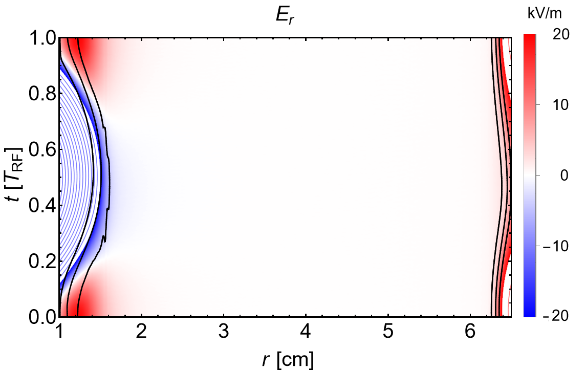
Figure 24: Spatio-temporally resolved electric field $E_{r}(r,t)$ for the magnetized magnetron discharge. The color shading is scaled to resolve the weak fields in the temporarily quasi-neutral regions; the additional contour lines have a separation of $\Delta E=20\,\mathrm{kV/m}$.

An alternative picture can be established by analyzing the motion of individual electrons. We assume a magnetic field $\boldsymbol{B}=B_{z}(r)\,\boldsymbol{e}_{z}$ and an RF modulated electric field $\boldsymbol{E}=E_{r}(r,t)\,\boldsymbol{e}_{r}$. For our numerical trajectory example, we take the magnetic field (2) and the electrical field from the simulations below, see Fig. 24. (The results of this section can thus be compared directly with the simulation outcome.) The motion along the magnetic field lines is simple: The coordinate $z$ moves uniformly in time, the velocity $v_{z}$ is constant:

$$\frac{\mathrm{d}z}{\mathrm{d}t}=v_{z},$$ (18)

$$\frac{\mathrm{d}v_{z}}{\mathrm{d}t}=0.$$ (19)

Consequently, also the kinetic energy of the motion along the magnetic field is constant:

$$\frac{\mathrm{d}\epsilon_{\parallel}}{\mathrm{d}t}\equiv\frac{\mathrm{d}\epsilon_{z}}{\mathrm{d}t}\equiv\frac{\mathrm{d}}{\mathrm{d}t}\left(\frac{1}{2}m_{\mathrm{e}}v_{z}^{2}\right)=0.$$ (20)

The motion in the $r$-$\theta$-plane is governed by the Lorentz force and the inertial pseudo-forces, with the former typically dominating the latter by an order of magnitude:

$$\frac{\mathrm{d}r}{\mathrm{d}t}=v_{r},$$ (21)

$$\frac{\mathrm{d}\theta}{\mathrm{d}t}=\frac{v_{\theta}}{r},$$ (22)

$$\frac{\mathrm{d}v_{r}}{\mathrm{d}t}=-\frac{e}{m_{\mathrm{e}}}(E_{r}+v_{\theta}B_{z})+\frac{v_{\theta}^{2}}{r},$$ (23)

$$\frac{\mathrm{d}v_{\theta}}{\mathrm{d}t}=\frac{e}{m_{\mathrm{e}}}v_{r}B_{z}-\frac{v_{r}v_{\theta}}{r}.$$ (24)

The kinetic energy in the $r$-$\theta$-plane is modulated by the power influx from the electric field. As expected, the Lorentz force and the inertial force do not contribute:

$$\frac{\mathrm{d}\epsilon_{\perp}}{\mathrm{d}t}\equiv\frac{\mathrm{d}}{\mathrm{d}t}\left(\epsilon_{r}+\epsilon_{\theta}\right)\equiv\frac{\mathrm{d}}{\mathrm{d}t}\left(\frac{1}{2}m_{\mathrm{e}}v_{r}^{2}+\frac{1}{2}m_{\mathrm{e}}v_{\theta}^{2}\right)=-ev_{r}E_{r}.$$ (25)

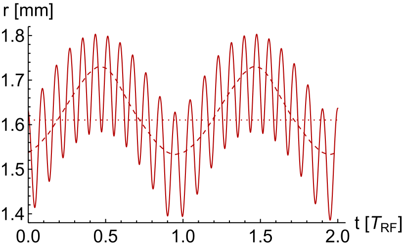
Figure 5: Solid red: Radial coordinate $r(t)$ of the sample trajectory followed over two RF periods. Dotted red: Reference radius $\hat{r}$. Dashed red: Position of the guiding center $\hat{r}-\hat{v}_{E\times B}(t)/\bar{\Omega}$.

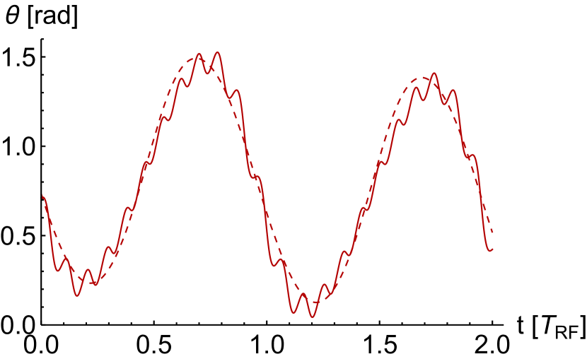
Figure 6: Solid red: Azimuthal coordinate $\theta(t)$ of the sample trajectory followed over two RF periods. Dashed red: Position of the guiding center $\hat{\theta}$.

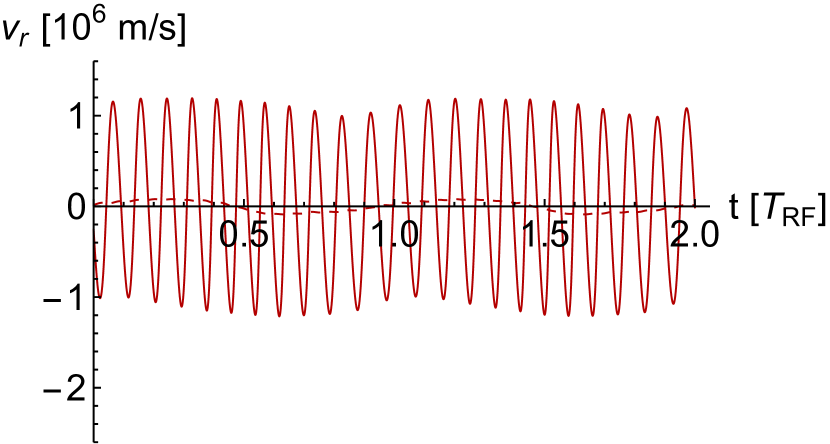
Figure 7: Solid red: Radial velocity $v_{r}$ of the sample trajectory recorded over two RF periods. Dashed red: Drift velocity due to polarization drift.

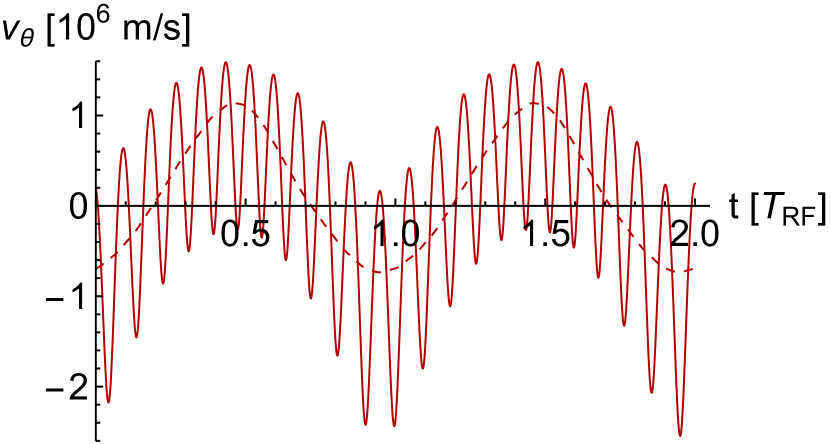
Figure 8: Solid red: Azimuthal Velocity $v_{\theta}$ of the sample trajectory recorded over two RF periods. Dashed red: Drift velocity due to $\boldsymbol{E}\!\times\!\boldsymbol{B}$ drift.

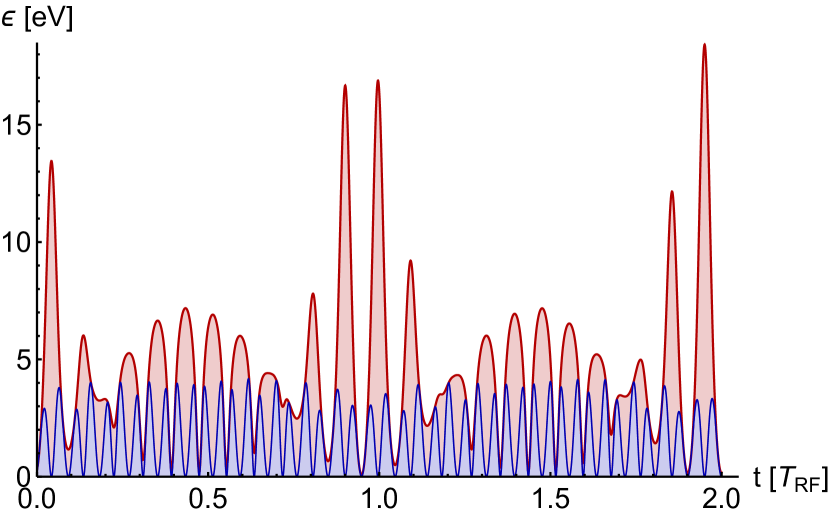
Figure 9: Kinetic particle energy in radial direction (blue) and in azimuthal direction (red) of the sample trajectory over two RF periods. The second curve shows constructive and destructive interference of gyro motion and drift.

A numerical integration of the cross-sectional equations of motion can easily be carried out. For a medium-energy particle in the strongly magnetized zone, Fig. 4 diplays the trajectory in the cross-sectional $r$-$\theta$-plane over a single RF period and over a stretch of 25 RF periods. It clearly shows a superposition of gyromotion and drift. Figs. 5 and 6 display the evolution of the coordinates $r(t)$ and $\theta(t)$ over two RF periods, respectively, while Figs. 7 and 8 show the velocities $v_{r}(t)$ and $v_{\theta}(t)$. Fig. 9 shows the corresponding kinetic energies.

It is instructive to compare the numerically calculated trajectories above with approximate solutions constructed by means of perturbation analysis. We apply a technique based on a series expansion in the ratio of the gyroradius to the discharge scale, $\eta=r_{\mathrm{L}}/|r-R_{\mathrm{E}}|\approx 0.1$. For a qualitative picture, it suffices to evaluate the power series up to the leading order in $\eta$. (Appendix A provides more mathematical details and formulates also higher order terms.) We start by noting that there is, due to the cylindrical symmetry, a strict constant of motion, the canonical momentum $p_{\theta}=rm_{\mathrm{e}}v_{\theta}-reA_{\theta}(r)$, where $A_{\theta}$ is the $\theta$-component of the magnetic vector potential $\mathbf{A}$. It can be used to define the temporally constant reference radius $\hat{r}$ of an electron trajectory via the relation $p_{\theta}\stackrel{{\scriptstyle!}}{{=}}-\hat{r}\,eA_{\theta}(\hat{r})$. In the numerical example, $\hat{r}=16.1\,\mathrm{mm}$.We use the circumflex also to denote the constant magnetic flux density $\hat{B}=B_{z}(\hat{r})=5.4\,\mathrm{mT}$ at the reference radius $\hat{r}$. The corresponding gyrofrequency is $\hat{\Omega}=e\hat{B}/m_{\mathrm{e}}=9.5\times 10^{8}\,\mathrm{s}^{-1}$.The temporally varying electric field strength at the reference point is termed $\hat{E}(t)=E_{r}(\hat{r},t)$;the corresponding drift speed is $\hat{v}_{E\times B}(t)=\hat{E}(t)/\hat{B}$. An approximate solution of the equations of motion can then be expressed as follows. Note the correspondence of (28) and (29) with (8) and (9) under the assumptions $\nu_{\mathrm{e}}\to 0$, $\omega\ll\omega_{\mathrm{ce}}$, and $\hat{\rho}\to 0$:

$$r=\hat{r}-\frac{\hat{v}_{E\times B}}{\hat{\Omega}}+\hat{\rho}\cos\bigl{(}\hat{\Omega}\,t+\hat{\phi}\bigr{)},$$ (26)

$$\theta=\hat{\theta}+\frac{\hat{\rho}}{\hat{r}}\sin\bigl{(}\hat{\Omega}\,t+\hat{\phi}\bigr{)},$$ (27)

$$v_{r}=-\frac{1}{\hat{\Omega}}\frac{\mathrm{d}\hat{v}_{E\times B}}{\mathrm{d}t}-\hat{\Omega}\,\hat{\rho}\,\sin\bigl{(}\hat{\Omega}\,t+\hat{\phi}\bigr{)},$$ (28)

$$v_{\theta}=-\hat{v}_{E\times B}(t)+\hat{\Omega}\,\hat{\rho}\,\cos\bigl{(}\hat{\Omega}\,t+\hat{\phi}\bigr{)}.$$ (29)

The gyroradius $\hat{\rho}$ is an adiabatic constant, i.e., independent of time, while the gyrophase offset $\hat{\phi}$ and the azimuth offset $\hat{\theta}$ exhibit a slow evolution. In the next order approximation, this is described as follows, with the prime indicating the derivative with respect to $\hat{r}$:

$$\frac{\mathrm{d}\hat{\phi}}{\mathrm{d}t}=\frac{3}{2}\left(\frac{1}{\hat{r}}-\frac{\hat{B}^{\prime}}{\hat{B}}\right)\hat{v}_{E\times B}+\frac{\hat{E}^{\prime}}{2B},$$ (30)

$$\frac{\mathrm{d}\hat{\theta}}{\mathrm{d}t}=-\frac{1}{\hat{r}}\hat{v}_{E\times B}.$$ (31)

The kinetic energy of the electron can be calculated as

$$\epsilon\approx\frac{1}{2} m_{\mathrm{e}}\hat{\Omega}^{2}\hat{\rho}^{2}+\frac{1}{2}m_{\mathrm{e}}\left(\hat{v}_{E\times B}(t)^{2}+\frac{1}{\hat{\Omega}^{2}}\left(\frac{\mathrm{d}\hat{v}_{E\times B}}{\mathrm{d}t}\right)^{2}\right)$$ (32)

$$+m_{\mathrm{e}}\hat{\Omega}\hat{\rho}\left(-\cos\bigl{(}\hat{\Omega}\,t+\hat{\phi}\bigr{)}\hat{v}_{E\times B}(t)+\sin\bigl{(}\hat{\Omega}\,t+\hat{\phi}\bigr{)}\frac{1}{\hat{\Omega}}\frac{\mathrm{d}\hat{v}_{E\times B}}{\mathrm{d}t}\right)+\frac{1}{2}m_{\mathrm{e}}v_{z}^{2}.$$

Obviously, the electron dynamics can be described as the superposition of a large-scale drift of the guiding center – first terms in (26) - (29) – and a small-scale gyromotion (last terms). The guiding center trajectories have a banana-like shape, which can be explained physically: The force $\boldsymbol{F}=-e\hat{E}\boldsymbol{e}_{r}$ perpendicular to $\boldsymbol{B}$ modulates the energy of the gyrating electron;it grows when the electron moves in the direction of $\boldsymbol{F}$ and decreases when it moves otherwise. The net effect is a drift $\boldsymbol{v}_{\mathrm{d}}=-\hat{v}_{E\times B}(t)\boldsymbol{e}_{\theta}$. The resulting shift in the azimuthal position $r\Delta\theta$ is of the order of $v_{E\times B}/\omega_{\mathrm{RF}}$. In contrast, the motion in the radial direction is of second order: Because the drift $\boldsymbol{v}_{\mathrm{d}}$ is RF modulated, it causes an acceleration that acts as a pseudo-force.The corresponding drift is known as the polarization drift lieberman_2005 , it has a phase shift of 90° and is an order of magnitude smaller than the $E\!\times\!B$ drift. The corresponding shift $\Delta\boldsymbol{r}_{\mathrm{p}}$ in the radial position is proportional to the electric field:

$$\boldsymbol{v}_{\mathrm{p}}=-m_{e}\frac{\mathrm{d}\hat{v}_{E\times B}}{\mathrm{d}t}\boldsymbol{e}_{\theta}\!\times\!\frac{\hat{\boldsymbol{B}}}{e\hat{B}^{2}}=-\frac{1}{\hat{\Omega}}\frac{\mathrm{d}\hat{v}_{E\times B}}{\mathrm{d}t}\,\boldsymbol{e}_{r},$$ (33)

$$\Delta\boldsymbol{r}_{\mathrm{p}}=-\frac{\hat{v}_{E\times B}}{\hat{\Omega}}\,\boldsymbol{e}_{r}=-\frac{m_{\mathrm{e}}\hat{E}}{e\hat{B}^{2}}\,\boldsymbol{e}_{r}.$$ (34)

The ratio $\Delta r_{\mathrm{p}}/r\Delta\theta$ thus scales as $\omega_{\mathrm{RF}}/\omega_{\mathrm{ce}}\ll 1$. The banana shape results from the curvature of the azimuthal coordinate lines. The trajectories somewhat resemble the banana-shaped trajectories of the guiding center of trapped particles in tokamaks, although the underlying drift mechanisms are of a different nature wesson_2011 . Note that the azimuthal drift velocity and the gyro speed are comparable. The azimuthal kinetic energy $\epsilon_{r}$ therefore shows destructive and constructive interference; values of nearly $20\,\mathrm{eV}$ can be reached, see Fig. 9.

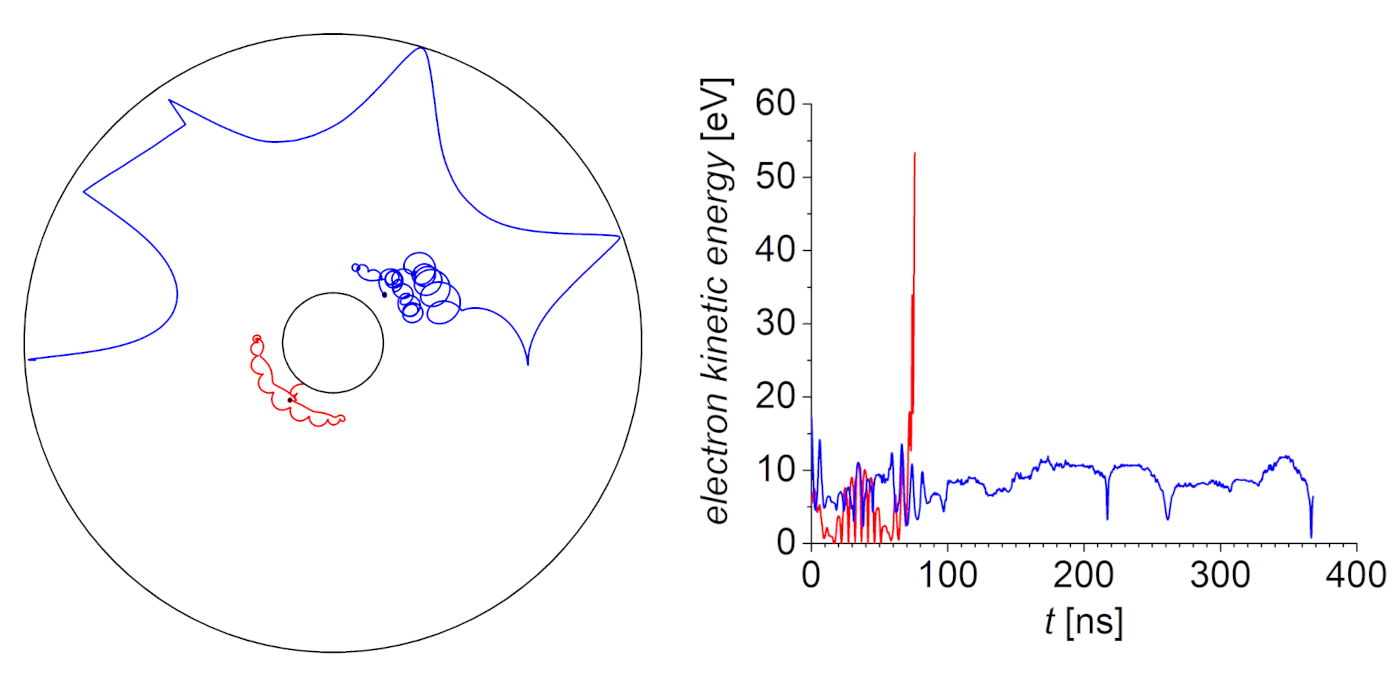
Figure 10: Orbits (left) and kinetic energies (right) of two typical electrons with a similar initial radial location but different initial velocities (see description in the text).

The approximate solution gives only a qualitative picture. Due to the strong non-uniformity of particularly the electric field at the sheath edge, finite Larmor radius effects play a role. In addition, the motion is strongly influenced by collisions. Fig. 10 (left) shows the orbits of two electrons taken from the self-consistent simulation described in section VII below.Both electrons start near the electrode (marked by black circles) during sheath collapse. The first electron (red) is initially trapped by the magnetic field. It experiences a modulated electric field, which is positive from $t=0\,\mathrm{ns}$ to $t=15\,\mathrm{ns}$, negative from $t=15\,\mathrm{ns}$ to $t=57\,\mathrm{ns}$,and then positive again. The corresponding azimuthal $\boldsymbol{E}\!\times\boldsymbol{B}$-drift results in a banana-like trajectory of the guiding center, the width of which is determined by the polarization drift.Fig. 10 (right) shows that the kinetic energy is also modulated. At $t=73\,\mathrm{ns}$ and $t=74\,\mathrm{ns}$,the electron undergoes elastic collisions which change its orbit and cause it to go to the electrode during the next phase. The other electron (blue) also remains initially trapped close to the electrode, despite collisions at $t=30\,\mathrm{ns}$ and $t=70\,\mathrm{ns}$. Between the elastic collisions, it experiences a strong electric field of changing polarity and changes its energy accordingly. A final collision at $t=100\,\mathrm{ns}$ scatters the particle near the grounded electrode where the magnetic field is weak. There it follows an orbit with a very large gyroradius and is repeatedly reflected by the potential of the grounded sheath.

V Kinetic description and velocity moments

For a complete picture of the processes in the discharge, the dynamics of the particles (including collisions and wall interactions) must be coupled to the evolution of the fields. In the low pressure regime of magnetrons, kinetic and non-local phenomena are expected, and a kinetic approach is to be adopted. The particle sector is described by a collection of Boltzmann equations for the distribution functions $f_{s}=f_{s}(r,v_{r},v_{\theta},v_{z},t)$, with $s=1\dots N_{\mathrm{s}}$. (Our specific calculations use $s\in\{\mathrm{e},\mathrm{i}\}$.) For the streaming term on the left, the equations of motion (18) are used, while the term on the right describes the action of collisions:

$$\frac{\partial f_{s}}{\partial t}+v_{r}\frac{\partial f_{s}}{\partial r}+\left(\frac{q_{s}}{m_{s}}\bigl{(}E_{r}+v_{\theta}B_{z}\bigr{)}+\frac{v_{\theta}^{2}}{r}\right)\frac{\partial f_{s}}{\partial v_{r}}-\left(\frac{q_{s}}{m_{s}}v_{r}B_{z}+\frac{v_{\theta}v_{r}}{r}\right)\frac{\partial f_{s}}{\partial v_{\theta}}=C(f_{s}).$$ (35)

Because of the small dimensions of the discharge and the relatively small electron density, the electrostatic approximation can be adopted. The radial electric field $E_{r}$ is the gradient of the electrostatic potential, $E_{r}=-\partial\Phi/\partial r$, and Poisson’s equation can be written as

$$-\varepsilon_{0}\frac{1}{r}\frac{\partial}{\partial r}r\frac{\partial\Phi}{\partial r}=\sum_{s=1}^{N_{\mathrm{s}}}q_{s}\int f_{s}\,\mathrm{d}v_{r}\,\mathrm{d}v_{\theta}\,\mathrm{d}v_{z}.$$ (36)

A direct solution of these equations with current computational resources is cumbersome. We thus employ ECCOPIC1S-M, a specialized member of our own ECCOPIC (Energy- and Charge-COnserving PIC) suite of GPU-parallelized energy and charge conserving particle-in-cell/ Monte Carlo collisions (PIC/MCC) codes Eremin2022 . ECCOPIC1S-M is an electrostatic 1d3v code for magnetized low pressure discharges in Cartesian, cylindrical, or spherical geometry. It contains several innovations over standard PIC/MCC. The particle positions and potentialvalues are found self-consistently during a time step, using the Crank-Nicolson method inherent to energy-conserving PIC/MCC schemes chen_2011 . The algorithm relaxes the criterion for the onset of the finite grid instability which causes numerical heating in conventional PIC/MCC if the cell size is greater than the Debye length Barnes2021 . The accuracy of the orbit integration is controlled by an adaptive sub-stepping technique. An external network with voltage source and blocking capacitor is fully integrated. The collisions are evaluated with the null collision method vahedi_1995 modified for GPUs mertmann_2011 ; the cross sections are adopted from Phelps phelps_1999 ; phelps_1994 .As the plasma density is low, Coulomb collisions are neglected. The ion-induced secondary electron emission coefficient was assumed to be $\gamma=0.1$ and the sticking coefficient $s=1$. For details on the implemented algorithms, see chen_2011 ; markidis_2011 ; Eremin2022 , for verification of the code family ECCOPIC and benchmarking, see turner_2013 ; charoy_2019 ; villafana_2021 .

The primary results of a PIC/MCC run are the electric potential values on the grid and the particle positions as functions of time. Single particle trajectories can be recorded as well. More insight into the dynamics can be obtained by reconstructing the velocity moments of the phase-space distribution function $f$. Defined abstractly as integrals over velocity space, they are realized in the simulation code as sums over all particles in the respective grid cells. To reduce noise, an average is taken over 1000 RF periods after convergence has been reached.Focusing on the electrons and suppressing the index $\mathrm{e}$, we list the electron density

$$n(r,t)=\int f(r,v_{r},v_{\theta},v_{z},t)\,\mathrm{d}^{3}v,$$ (37)

the mean electron velocities in the directions $r$ and $\theta$,

$$u_{r}(r,t)=\frac{1}{n}\int v_{r}f(r,v_{r},v_{\theta},v_{z},t)\,\mathrm{d}^{3}v,$$ (38)

$$u_{\theta}(r,t)=\frac{1}{n}\int v_{\theta}f(r,v_{r},v_{\theta},v_{z},t)\,\mathrm{d}^{3}v,$$ (39)

and the non-vanishing elements of the pressure tensor,

$$p_{rr}(r,t)=\int m(v_{r}-u_{r})(v_{r}-u_{r})f(r,v_{r},v_{\theta},v_{z},t)\,\mathrm{d}^{3}v,$$ (40)

$$p_{r\theta}(r,t)=\int m(v_{r}-u_{r})(v_{\theta}-u_{\theta})f(r,v_{r},v_{\theta},v_{z},t)\,\mathrm{d}^{3}v,$$ (41)

$$p_{\theta\theta}(r,t)=\int m(v_{\theta}-u_{\theta})(v_{\theta}-u_{\theta})f(r,v_{r},v_{\theta},v_{z},t)\,\mathrm{d}^{3}v,$$ (42)

$$p_{zz}(r,t)=\int mv_{z}v_{z}f(r,v_{r},v_{\theta},v_{z},t)\,\mathrm{d}^{3}v.$$ (43)

Furthermore, we define the following moments of the collision integral,

$$S=\int C(f_{s})\,\mathrm{d}^{3}v,$$ (44)

$$F_{r}=\int mv_{r}\,C(f_{s})\,\mathrm{d}^{3}v,$$ (45)

$$F_{\theta}=\int mv_{\theta}\,C(f_{s})\,\mathrm{d}^{3}v.$$ (46)

Multiplying the kinetic equation with $1$, $mv_{r}$ and $mv_{\theta}$ and integrating over velocity space yields the particle balance and the momentum balances in the directions of $r$ and $\theta$:

$$\frac{\partial n}{\partial t}+\frac{1}{r}\frac{\partial}{\partial r}\left(rnu_{r}\right)=S,$$ (47)

$$\frac{\partial}{\partial t}(mnu_{r})+\frac{1}{r}\frac{\partial}{\partial r}\left(r\left(mnu_{r}^{2}+p_{rr}\right)\right)-\frac{1}{r}\left(p_{\theta\theta}+mnu_{\theta}^{2}\right)=-en\left(E_{r}+u_{\theta}B_{z}\right)+F_{r},$$ (48)

$$\frac{\partial}{\partial t}(mnu_{\theta})+\frac{1}{r^{2}}\frac{\partial}{\partial r}\left(r^{2}\left(mnu_{r}u_{\theta}+p_{r\theta}\right)\right)=enu_{r}B_{z}+F_{\theta}.$$ (49)

VI PIC/MCC results: Reference case without magnetic field

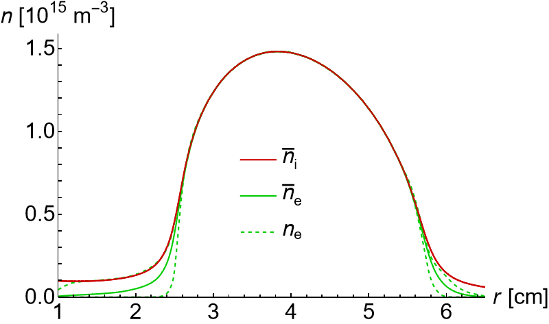
Figure 11: RF period-averaged ion density $\bar{n}_{\mathrm{i}}(r)$ (solid red) and electron density $\bar{n}_{\mathrm{e}}(r)$ (solid green) of the unmagnetized reference discharge. The dashed green lines denote electron densities $n_{\mathrm{e}}(r,t)$ at the sheath minimum (t = 0) and maximum (t = TRF/2), respectively.

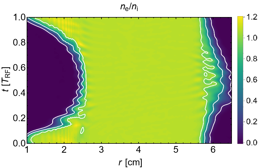
Figure 12: Spatio-temporally resolved ratio of the electron density $n_{\mathrm{e}}(r,t)$ to the ion density $n_{\mathrm{i}}(r,t)$for the unmagnetized reference discharge. The plasma-sheath transition is indicated by the white contours $n_{\mathrm{e}}/n_{\mathrm{i}}=0.1,0.5,0.9$ (from inside to outside) which will be used also in other figures.

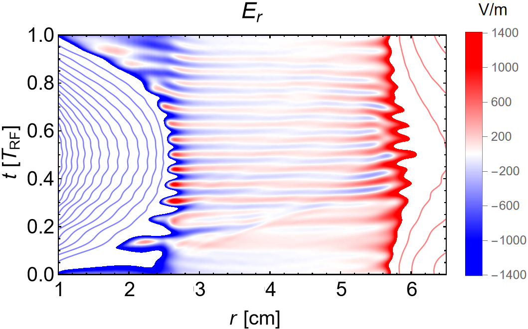
Figure 13: Spatio-temporally resolved electric field $E_{r}(r,t)$ for the unmagnetized reference discharge. The color shading is scaled to resolve the weak fields in the plasma; the additional contour lines have a separation of $\Delta E=5000\,\mathrm{V/m}$.

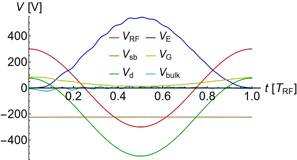
Figure 14: Phase-resolved curves of the applied source voltage $V_{\mathrm{RF}}(t)$, the self bias voltage $V_{\mathrm{sb}}(t)$, the total discharge voltage $V_{\mathrm{d}}(t)$, the sheath voltages $V_{\mathrm{E}}(t)$ and $V_{\mathrm{G}}(t)$, and the voltage drop $V_{\mathrm{bulk}}(t)$ over the plasma bulk for the unmagnetized reference case.

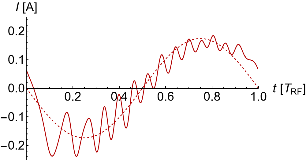
Figure 15: Discharge current $I(t)$ of the unmagnetized case (solid) in comparison with the discharge current of the corresponding Drude model (dashed).

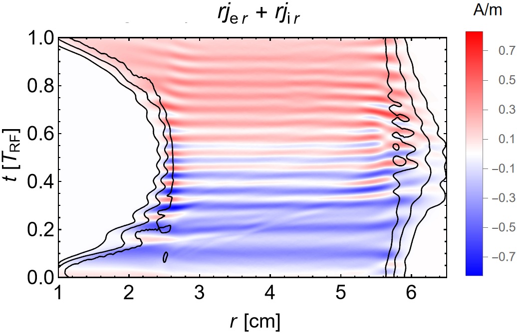
Figure 16: Radially weighted particle current $rj_{r}(r,t)$ of the unmagnetized reference discharge.

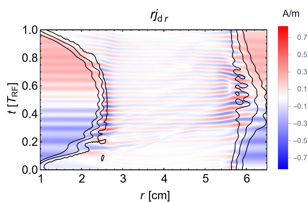
Figure 17: Radially weighted displacement current $rj_{\mathrm{d}r}(r,t)$ of the unmagnetized reference discharge.

For reference, let us first consider the simpler unmagnetized case. It follows the logic of all RF-driven capacitive discharges: The plasma self-organizes into the quasineutral bulk and two electron-depleted sheaths in front of the driven and grounded electrodes, respectively. Fig. 11 shows the phase-averaged densities of the electrons $\bar{n}_{\mathrm{e}}(r)$ and the ions $\bar{n}_{\mathrm{i}}(r)$ and theelectron densities $n_{\mathrm{e}}(r,t)$ at $t=0$ and $t=T_{\mathrm{RF}}/2$. The peak density is $n=1.5\!\times\!10^{15}\,\mathrm{m}^{-3}$. Fig. 12 provides a map of the ratio $n_{\mathrm{e}}(r,t)/\bar{n}_{\mathrm{i}}(r)$, Fig. 13 a map of the electric field $E_{r}(r,t)$. The electrons can follow the electric field, their plasma frequency $\omega_{\mathrm{pe}}=2.2\!\times\!10^{9}\,\mathrm{s}^{-1}$ (center) or $\omega_{\mathrm{pe}}=6.5\!\times\!10^{8}\,\mathrm{s}^{-1}$ (electrode sheath) is larger than the radio frequency $\omega_{\mathrm{RF}}=8.5\!\times\!10^{7}\,\mathrm{s}^{-1}$. The ions, in contrast, are almost unmodulated and react only on the phase-averaged field;their plasma frequency is $\omega_{\mathrm{pi}}=8.0\!\times\!10^{6}\,\mathrm{s}^{-1}$ (center) or $\omega_{\mathrm{pi}}=2.4\!\times\!10^{6}\,\mathrm{s}^{-1}$ (electrode sheath). Fig. 14 shows the applied voltage, the discharge and sheaths voltages, and the bias voltage. The RF current $I(t)$ that flows through the discharge – see Fig. 15 – is spatially constant, it is the sum of the (small) ion current, the electron current, and the displacement current. Figs. 16 and 17 show spatio-temporally resolved maps of the components of this current. The factor $2\pi r$ reflects the cylindrical symmetry of the device, $H$ is its nominal height:

$$I(t)=2\pi rHj(r,t)=2\pi rH\left(en_{\mathrm{i}}u_{\mathrm{i}}-en_{\mathrm{e}}u_{\mathrm{e}}+\varepsilon_{0}\frac{\partial E_{r}}{\partial t}\right).$$ (50)

Due to the cylindrical device geometry, the current densities at the driven and the grounded electrode scale like $j_{\mathrm{E}}\!:\!j_{\mathrm{G}}=R_{\mathrm{G}}\!:\!R_{\mathrm{E}}=6.5\!:\!1$. This makes the discharge strongly asymmetric; the inner sheath is much wider ($\bar{s}_{\mathrm{E}}=1.1\,\mathrm{cm}$) than the grounded outer sheath ($\bar{s}_{\mathrm{G}}=0.56\,\mathrm{cm}$). To understand the electric behavior of the discharge, it is useful to consult a simplified model which analyzes the evolution of the charges in the driven and grounded sheath,

$$Q_{E}=H\int_{R_{\mathrm{E}}}^{R_{\mathrm{C}}}e(n_{\mathrm{i}}-n_{\mathrm{e}})\,2\pi r\,\mathrm{d}r,$$ (51)

$$Q_{\mathrm{G}}=H\int_{R_{\mathrm{C}}}^{R_{\mathrm{G}}}e(n_{\mathrm{i}}-n_{\mathrm{e}})\,2\pi r\,\mathrm{d}r.$$ (52)

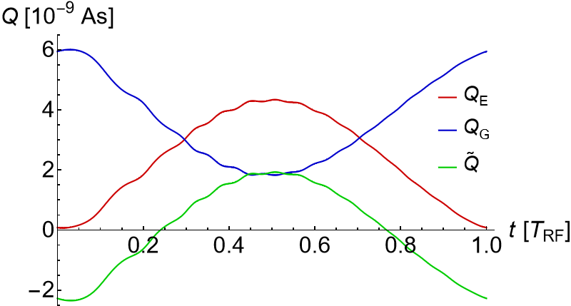
Figure 18: Charges of the electrode sheath $Q_{\mathrm{E}}(t)$ and the ground sheath $Q_{\mathrm{G}}(t)$ together with the average-free integral $\tilde{Q}(t)$ of the current $I(t)$ for the unmagnetized reference case.

The RF current modulates the charges of the two sheaths. Neglecting small terms related to charge carrier losses to the electrodes, we write as follows, where the charge quantity $\tilde{Q}(t)$ is the phase-average-free integral of $-I(t)$, see Fig. 18:

$$\frac{\mathrm{d}Q_{\mathrm{E}}}{\mathrm{d}t}=-\frac{\mathrm{d}Q_{\mathrm{G}}}{\mathrm{d}t}=-I(t)=\frac{\mathrm{d}\tilde{Q}}{\mathrm{d}t}.$$ (53)

The voltage drop over the discharge $V(t)$ is equal to the sum of the applied RF voltage $V_{\mathrm{RF}}(t)$ and the nearly constant self-bias $V_{\mathrm{sb}}=-224\,\mathrm{V}$. Assuming that the sheath voltages $V_{\mathrm{E}}$ and $V_{\mathrm{G}}$ are functions of $Q_{\mathrm{E}}$ and $Q_{\mathrm{G}}$, respectively (Fig. 19), and neglecting all other electric fields, a voltage balance can be formulated. Here, the offset charges $\bar{Q}_{\mathrm{E}}$, $\bar{Q}_{\mathrm{G}}$ and the self bias $V_{\mathrm{sb}}$are constants which self-adjust so that the floating condition holds:

$$-V_{\mathrm{E}}\left(\bar{Q}_{\mathrm{E}}+\tilde{Q}(t)\right)+V_{\mathrm{G}}\left(\bar{Q}_{\mathrm{G}}-\tilde{Q}(t)\right)-V_{\mathrm{sb}}=V_{\mathrm{RF}}\cos(\omega t).$$ (54)

This quasistatic model explains much of the electrical behavior: The sheath voltages and the bias voltage are determined by the voltage $V_{\mathrm{RF}}(t)$. The periodic charging and discharging of the sheaths gives rise to the discharge current $I(t)$. However, the model over-idealizes: Its predicts that the charges and voltages are exact functions of the RF voltage $V_{\mathrm{RF}}(t)$,and that the discharge current $I(t)$, being a derivative of $\tilde{Q}(t)$, has an exact 90° phase shift. This would imply zero net heating. (See the appendix of SchulzeDonkoLafleurWilczekBrinkmann2018 for details on this argument.)

In reality, and in the results of the PIC/MCC simulation, the current-voltage phase angle is not exactly 90° but very close to it,

$$\cos\varphi=\frac{1}{T}\int_{0}^{T}IV\,\mathrm{d}t\Bigg{/}\sqrt{\frac{1}{T}\int_{0}^{T}I^{2}\,\mathrm{d}t\,\frac{1}{T}\int_{0}^{T}V^{2}\,\mathrm{d}t}=0.0439=\cos 87.5\text{\textdegree},$$ (55)

and the phase-averaged dissipation is not zero but

$$\bar{P}=\ \frac{1}{T}\int_{0}^{T}IV\,\mathrm{d}t=1.22\,\mathrm{W}.$$ (56)

Responsible for the non-vanishing heating are, in fact, the small “other electric fields” that were neglected in the voltage balance (54). These small fields are needed to locally drive the current density $j(r,t)$ which corresponds to the globally determined discharge current $I(t)$. (They are also not well represented in the cold plasma model whose predictions of $\phi=89.96$° for the phase angle and $\bar{P}=0.018\,\mathrm{W}$ for the Ohmically dissipated power are unrealistic. However, the cold plasma model explains well the current oscillations related to the PSR;the predicted value of $\omega_{\mathrm{PSR}}=1.29\,\times\,10^{9}\,\mathrm{s}^{-1}$ agrees with the outcome of the simulations.) In the vicinity of the sheaths, where the local plasma frequency $\omega_{\mathrm{pe}}(r)$ is close to $\omega_{\mathrm{PSR}}$,also Langmuir oscillations occur Wilczek2020 ; see the phase-resolved maps of the electric field $E_{r}(r,t)$,the particle current $j_{r}(r,t)$, and the displacement current $j_{\mathrm{d}}(r,t)$. The hallmark of Langmuir oscillations is a 180° degree phase shift between $j_{r}$ and $j_{\mathrm{d}}$.

Of the power $\bar{P}=1.22\,\mathrm{W}$ provided by the RF source, $\bar{P}_{\mathrm{i}}=0.91\,\mathrm{W}$ are absorbed by the ions and $\bar{P}_{\mathrm{e}}=0.31\,\mathrm{W}$ by the electrons. The energy transfer to the ions takes place in the sheaths and can be described in terms of the period-averaged field $\bar{E}_{r}$. The energy exchange between the electric field and the electrons, however, is a complex spatio-temporal phenomenon, involving both the RF modulation and the self-excited PSR. Insight is gained from a velocity moment analysis of the kinetic equation surendra_1993 ; SchulzeDonkoLafleurWilczekBrinkmann2018 . We solve the momentum balance (48) for the electric field which then can be separated into the inertia field, the pressure field,and the collisional field:

$$E_{r} =-\frac{1}{en}\left(\frac{\partial}{\partial t}(mnu_{r})+\frac{1}{r}\frac{\partial}{\partial r}\left(rmnu_{r}^{2}\right)-\frac{mnu_{\theta}^{2}}{r}\right)-\frac{1}{ren}\left(\frac{\partial}{\partial r}\left(rp_{rr}\right)-p_{\theta\theta}\right)+\frac{\dot{\pi}_{r}}{en}$$ (57)

$$\equiv E_{\mathrm{i}r}+E_{\mathrm{p}r}+E_{\mathrm{c}r}.$$

Multiplying by $rj_{r}=-renu_{r}$, we establish the mechanical energy balance and obtain a split of the radially weighted electron power dissipation $rP_{\mathrm{e}r}$, see Fig. 20,

$$rP_{\mathrm{e}r}=rj_{e}E_{r}= \;rmu_{r}\left(\frac{\partial}{\partial t}(nu_{r})+\frac{1}{r}\frac{\partial}{\partial r}\left(rnu_{r}^{2}\right)-\frac{nu_{\theta}u_{\theta}}{r}\right)+u_{r}\left(\frac{\partial}{\partial r}\left(rp_{rr}\right)-r\frac{p_{\theta\theta}}{r}\right)-ru_{r}\dot{\pi}_{r}$$

$$\equiv \;rP_{\mathrm{i}r}+rP_{\mathrm{p}r}+rP_{\mathrm{c}r}.$$ (58)

There is almost no electron heating in the plasma bulk; virtually all RF power is absorbed in the temporarily quasineutral sections of the sheaths. All the heating processes discussed in section I are present, but are of different importance. “Classical” Ohmic heating is weak: The collisional term $rP_{\mathrm{c}}$ contributes only 25 % to $rP_{\mathrm{e}}$, not surprising at the small gas pressure of only $p=0.5\,\mathrm{Pa}$. The inertia term $rP_{\mathrm{i}}$ can be momentarily large but is small on average.(This reflects that inertia forces are often non-dissipative: Electrons accelerated during one half phase of PSR osillations can be decelerated in the other and feed their energy back.) The main contribution is thus embodied in the pressure term $P_{\mathrm{p}r}$.

A kinetic analysis can refine this picture. Immediately after sheath collapse, in the interval $t=0.02\,T_{\mathrm{RF}}$ to $t=0.14\,T_{\mathrm{RF}}$, the electrode sheath expands with a speed of $u_{\mathrm{s}}\approx 2\times 10^{6}\,\mathrm{m/s}$, This high speed arises from a synergy of the RF modulation and the PSR oscillation excited at the moment of sheath collapse czarnetzki_2006 . The fast moving sheath reflects the incoming electrons according to $v\to 2u_{\mathrm{s}}-v$. A group of energetic electrons forms, which, further accelerated by the ambipolar field of the presheath, propagate beam-like towards the grounded electrode. This can be seen in Fig. 21 which displays the radially weighted, spatio-temporally resolved profile of the ionization term. Before the grounded electrode, the energetic beam is stopped by the ambipolar field and by the retreating sheath, giving rise to a negative power density. However, before reaching that region, some of them have lost their directed energy already by collisions in the bulk, so that even if the rest is fully decelerated by the opposite sheath, the period-averaged energy transfer rate is positive. In the second half of the RF period, the sheaths switch roles, but with less effect on the heating process, since the sheath before the grounded electrode is less strongly modulated. Another source of temporal asymmetry can be attributed to different electron temperatures during sheath expansion and collapse, also resulting in a positive period-averaged power absorption SchulzeDonkoDerzsiKorolovSchuengel2015 ; SchulzeDonkoLafleurWilczekBrinkmann2018 . Heating is therefore substantial in two situations: When there is a violent acceleration of a significant fraction of particles at the sheath edge, or at the sheath-presheath boundary where a significant temporally asymmetric ambipolar field is present SchulzeDonkoDerzsiKorolovSchuengel2015 .

VII Case with magnetic field

We now turn to the more complex magnetized case. (Fig. 1 gives a true-to-scale schematic.)Also this discharge self-organizes into a quasineutral bulk and two electron-depleted sheaths in front of the driven and grounded electrodes, respectively. Its plasma density, however,is $7.5$ times higher, the peak density is $n_{\mathrm{max}}=1.24\!\times\!10^{16}\,\mathrm{m}^{-1}$. The sheaths are thinner by nearly a factor of four, $\bar{s}_{\mathrm{E}}=0.32\,\mathrm{cm}$ and $\bar{s}_{\mathrm{G}}=0.14\,\mathrm{cm}$. Fig. 22 shows the phase-averaged densities $\bar{n}_{\mathrm{i}}(r)$ and $\bar{n}_{\mathrm{e}}(r)$ along with snapshots of $n_{\mathrm{e}}(r,t)$ at the phases $t=0$ and $t=T_{\mathrm{RF}}/2$.

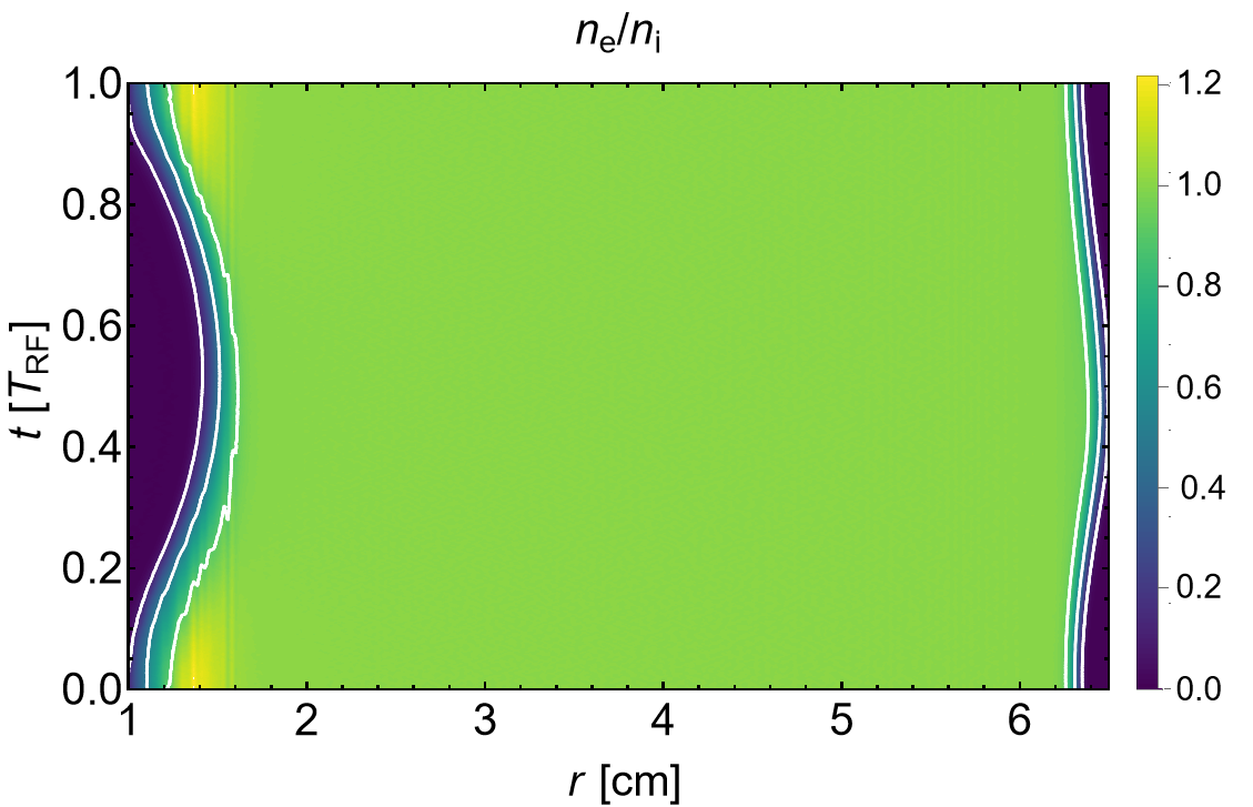
Figure 23: Spatio-temporally resolved ratio of the electron density $n_{\mathrm{e}}(r,t)$ to the ion density $n_{\mathrm{i}}(r,t)$for the magnetized discharge. The plasma-sheath transition is indicated by the white contours $n_{\mathrm{e}}/n_{\mathrm{i}}=0.9,0.5,0.1$ (from inside to outside) which will be used also in other figures.

Fig. 23 provides a map of the ratio $n_{\mathrm{e}}(r,t)/\bar{n}_{\mathrm{i}}(r)$, Fig. 24 a map of the electric field $E_{r}(r,t)$. Again, the electrons can follow the field, their plasma frequency is $\omega_{\mathrm{pe}}=5.7\!\times\!10^{9}\,\mathrm{s}^{-1}$ (center) or $\omega_{\mathrm{pe}}=2.2\!\times\!10^{9}\,\mathrm{s}^{-1}$ (electrode sheath), while the ion component is essentially unmodulated, $\omega_{\mathrm{pi}}=2.1\!\times\!10^{7}\,\mathrm{s}^{-1}$ (center) or $\omega_{\mathrm{pi}}=8.1\!\times\!10^{6}\,\mathrm{s}^{-1}$ (electrode sheath).

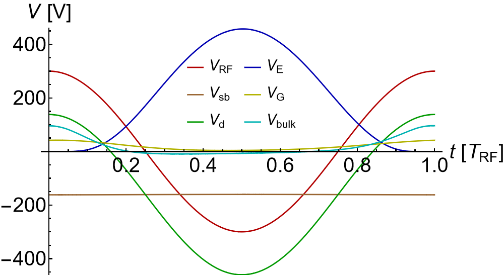
Figure 25: Phase-resolved curves of the applied source voltage $V_{\mathrm{RF}}(t)$, the self bias voltage $V_{\mathrm{sb}}(t)$, the total discharge voltage $V_{\mathrm{d}}(t)$, the sheath voltages $V_{\mathrm{E}}(t)$ and $V_{\mathrm{G}}(t)$, and the voltage drop $V_{\mathrm{bulk}}(t)$ over the plasma bulk for the magnetized case.

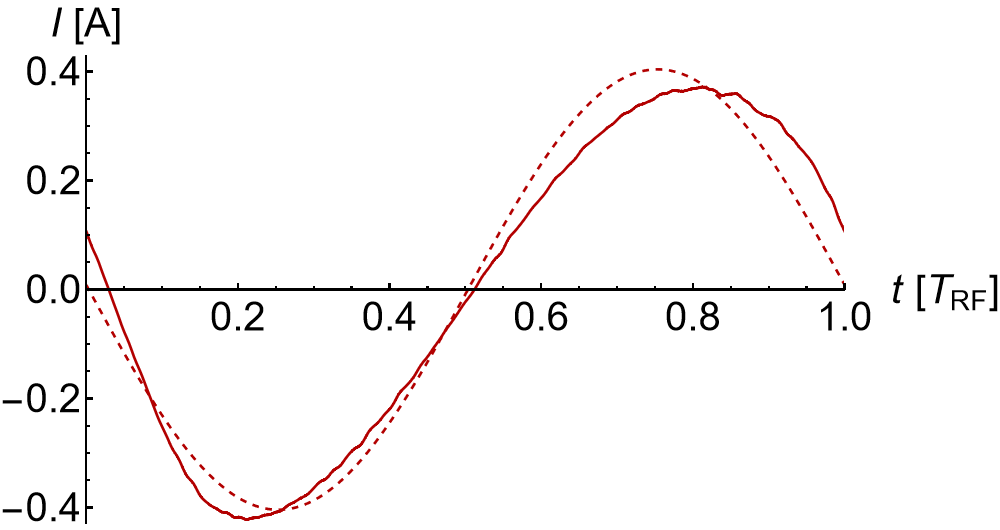
Figure 26: Discharge current $I(t)$ of the magnetized case (solid) in comparison with the discharge current of the corresponding Drude model (dashed).

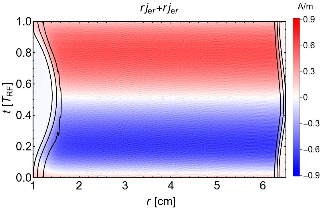
Figure 27: Radially weighted particle current $rj_{r}(r,t)$ in the magnetized case.

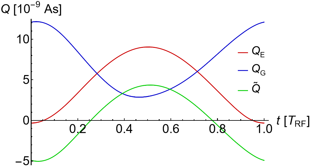
Figure 30: Charges of the electrode sheath $Q_{\mathrm{E}}(t)$ and the ground sheath $Q_{\mathrm{G}}(t)$ together with the average-free integral $\tilde{Q}(t)$ of the current $I(t)$ for the magnetized case.

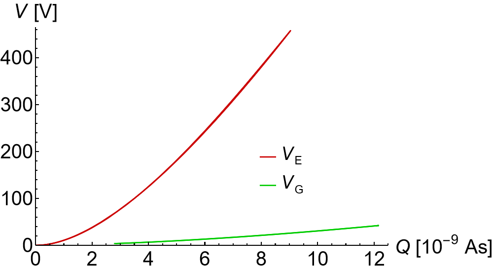
Figure 31: Charge-voltage curves $V_{\mathrm{E}}(Q)$ of the electrode sheath and $V_{\mathrm{G}}(Q)$ of the grounded sheath of the magnetized case.

Fig. 25 shows the voltages. At first glance, not much has changed compared to the reference.The applied voltage $V_{\mathrm{RF}}(t)$ is the same. The discharge voltage $V_{\mathrm{d}}(t)$, the sheath voltages $V_{\mathrm{E}}(t)$ and $V_{\mathrm{G}}(t)$, and the self bias $V_{\mathrm{sb}}(t)$ are similar. The bulk voltage $V_{\mathrm{b}}(t)$ remains small.Obviously, the discharge is capacitive as well, and the quasi-static analysis (54) still applies. In fact, it is now even more applicable: Because of the higher value of $\omega_{\mathrm{PSR}}$, the PSR is no longer excited by the sheath nonlinearities, and the total current $I(t)=2\pi Hrj(r,t)$ is better captured by the quasi-static model or the Drude model, Fig. 26. As shown in Figs. 27 and 28,it is carried by the electrons in the bulk and flows as displacement current in the sheaths. (Due to the absence of PSR oscillations, there is almost no displacement current in the bulk.)In contrast to the unmagnetized case, there is now also an azimuthal current $j_{\theta}$, see Fig. 29. The waveforms of the sheath charges are similar to those of the unmagnetized case, Fig. 30. They are, however, larger by a factor of 2. This ratio, which reflects the higher plasma densityand the thinner sheaths of the magnetized case, is also visible in the amplitude of the current and in the form of the charge voltage relations $V_{\mathrm{E}}(Q)$ and $V_{\mathrm{G}}(Q)$ shown in Fig. 31.

The simulation determines the current-voltage phase angle to $\cos\varphi=\cos 83.5\text{\textdegree}=0.113$ and the dissipated RF power to $\bar{P}=6.76\,\mathrm{W}$. (The Drude model, with $\cos\varphi=\cos 88.8\text{\textdegree}=0.021$ and $\bar{P}=1.30\,\mathrm{W}$ is far off.) $\bar{P}_{\mathrm{i}}=3.98\,\mathrm{W}$ is taken by the ions, $\bar{P}_{\mathrm{e}}=2.78\,\mathrm{W}$ by the electrons. The power input ratio matches the density ratio, $n_{\mathrm{max}}\mathrm{(M)}/n_{\mathrm{max}}\mathrm{(U)}\approx\bar{P}_{\mathrm{e}}\mathrm{(M)}/\bar{P}_{\mathrm{e}}\mathrm{(U)}\approx 8$. The plasma density of the magnetized case is higher because the heating is more efficient. We will demonstrate that it also has a very different physical character.

As in the unmagnetized reference case, the heating mechanism is related to the electric field in the ambipolar zone which is neglected in the quasi-static analysis and which is only poorly represented by the Drude model, see Fig. 24. Its individual components can be analyzed by solving the radial momentum balance (48) with respect to the electric field:

$$\!\!\!\!\!E_{r} =-\frac{1}{en}\!\left(\frac{\partial}{\partial t}(mnu_{r})+\frac{1}{r}\frac{\partial}{\partial r}(rmnu_{r}^{2})-\frac{mnu_{\theta}^{2}}{r}\right)-\frac{1}{ren}\!\left(\frac{\partial}{\partial r}\left(rp_{rr}\right)-p_{\theta\theta}\!\right)-u_{\theta}B_{z}+\frac{F_{r}}{en}$$

$$\equiv E_{\mathrm{i}}+E_{\mathrm{p}}+E_{\mathrm{H}}+E_{\mathrm{c}}.$$ (59)

The terms on the right can be obtained from the simulation. Two contributions dominate, the pressure field $E_{\mathrm{p}}$ and the Hall field $E_{\mathrm{H}}$. The pressure field appears at the electron edges of both sheaths and points outward, i.e., is negative around $s_{\mathrm{E}}(t)$ and positive around $s_{\mathrm{G}}(t)$. As in the unmagnetized case, it acts as an indicator of the beginning depletion field with which the electrons are roughly in Boltzmann equilibrium. The Hall field $E_{\mathrm{H}}$ reflects the Lorentz force and appears only in the magnetized zone. It has a 180° phase shift with respectto the electron edge $s_{\mathrm{E}}$. This can be explained in terms of the single-particle picture above: As (34) shows, a positive (reversed) field is needed to move electrons to smaller values of $r$ and a negative one to push them in the opposite direction.) There is thus a positive interference between $E_{\mathrm{p}}$ and $E_{\mathrm{H}}$ at the time of the sheath maximum and a cancellation around time of the the sheath minimum. However, as $E_{\mathrm{H}}$ is also active where quasineutrality holds, a strong positive field appears during the sheath minimum in the zone $1\,{\rm cm}\leq r\leq 2\,{\rm cm}$. The other electric field terms on the right of (VII) – reflecting the influence of electron inertia and collisions – are much smaller (see WangWenHartmannDonkoDerzsiWangSongWangSchulze2020 ). The dominance of the pressure field and the Hall field can also be detected in Fig. 32 which displays a phase-resolved map of the radiallyweighted electron power input $rP_{\mathrm{e}}=rj_{\mathrm{e}r}E_{r}$. Its individual constituents, defined on the basis of the electrical field analysis (VII), are displayed in Fig. 34:

$$\!\!\!\!\!rP_{r} =mu_{r}\!\left(r\frac{\partial}{\partial t}(nu_{r})+\frac{\partial}{\partial r}\left(rnu_{r}^{2}\right)-nu_{\theta}^{2}\right)+u_{r}\left(\frac{\partial}{\partial r}\left(rp_{rr}\right)-p_{\theta\theta}\right)-rj_{r}u_{\theta}B_{z}-ru_{r}\dot{\pi}_{r}$$

$$\equiv rP_{\mathrm{i}r}+rP_{\mathrm{p}r}+rP_{\mathrm{H}}+rP_{\mathrm{c}r}$$ (60)

The pressure term $P_{\mathrm{p}r}$ appears only in the thin transition zones around the electron edges; its value is positive when the sheaths are expanding and negative when they are retracting.The phase average is close to zero. The Hall term $P_{\mathrm{H}}$ is only active in the magnetized region, it is negative just after the sheath collapse and positive just before. The other contributions to the power balance are essentially negligible.

The Hall contribution $P_{\mathrm{H}}$ does not correspond to true power dissipation, as magnetic fields do not do any work and cannot contribute to heating. Instead, the term represents a flow of mechanical energy conducted from radial to azimuthal degrees of freedom and back.This view is supported by the following equation which is obtained by multiplying the azimuthal momentum balance (49) with $u_{\theta}$:

$$renu_{\theta}u_{r}B_{z} =u_{\theta}\!\left(r\frac{\partial}{\partial t}(mnu_{\theta})+\frac{1}{r}\frac{\partial}{\partial r}\left(r^{2}mnu_{r}u_{\theta}\right)\right)+u_{\theta}\frac{1}{r}\frac{\partial}{\partial r}\left(r^{2}p_{r\theta}\right)-ru_{\theta}\dot{\pi}_{\theta}$$ (61)

$$=rP_{\mathrm{i}\theta}+rP_{\mathrm{p}\theta}+rP_{\mathrm{c}\theta}$$

The term on the left is the negative of $P_{\mathrm{H}}$; it acts as power source for the azimuthal motion. Fig. 34 shows the three contributions on the right. To begin with the least important one: The term $P_{\mathrm{p}\theta}$ reflects the shear component of the pressure tensor and is linked to the collisionless effect of gyroviscosity: Radial transport of the axial momentum component caused by electron gyration hazeltine_2004 . Physically, and by numerical value, it is rather insignificant. The term $P_{\mathrm{i}\theta}$ is associated with electron inertia and reflects the periodic acceleration and deceleration of the electrons related to the $\boldsymbol{E}\!\times\!\boldsymbol{B}$ drift. During the field growth before the sheath collapse, energy is transferred to the electrons; after the collapse, is transferred back. This energizing mechanism is collisionless; it was already captured in the single-particle view. It generates a strong electron beam in the azimuthal direction, with a velocity that may exceed the thermal velocity significantly. (Even if the drift speed $v_{E\times B}$ is not larger than the thermal velocity but comparable to it, the kinetic energy can be up to four times larger than the thermal energy alone when the gyro motion and the drift have the same direction.)A sizable number of electrons close to the powered electrode can therefore reach energies in the inelastic range, so that they can participate directly in excitation or ionization processes. This is seen in the term $P_{\mathrm{c}\theta}$ and in the ionisation rate shown in Fig. 35. The confining effect of the magnetic field prevents the electrons from being ejected from the magnetized zone, allowing them to experience large electric fields over a long period of time. Note that the number of energetic electrons in such a zone is increased by the production of new electrons via the ionization process. Such electrons experience the same strong electric field and thus gain the same large $\mathbf{E}\!\times\!\mathbf{B}$ azimuthal drift velocity resulting in a large total kinetic energy. Under a sufficiently large ionization probability during a time interval when an electron feels a large electric field close to the powered electrode, this might significantly enhance the ionization efficiency by creating an ionization avalanche.

The findings are supported by the graphs of Fig. 36, which illustrate the electron velocity distribution in the $(v_{r},v_{\theta})$ plane of the velocity space for different phases of the RF cycle. The electrons were sampled from a segment close to the powered electrode, $1\,{\rm cm}\leq r\leq 2\,{\rm cm}$, where most of the energetic electrons are produced. (Secondary electrons are not shown.) The velocity range is the interval $[-v_{\mathrm{max}},v_{\mathrm{max}}]$, $v_{\mathrm{max}}=4.2\times 10^{6}\,{\rm m/s}$ corresponds to $50\,{\rm eV}$. The boundary between the elastic and inelastic energy range is shown as a magenta circle. At $t=0$, all electrons experience a strong positive (“reversed”) electric field which generates a fast $\boldsymbol{E}\!\times\!\boldsymbol{B}$ drift in the negative $\theta$ direction (Fig. 36a). A substantial fraction of electrons is pushed beyond the inelastic energy threshold. When the powered electrode sheath expands – we chose the moment $t=0.25\,T_{\mathrm{RF}}$ –, the electric field at the sheath edge changes polarity and the $\boldsymbol{E}\!\times\!\boldsymbol{B}$ drift becomes small for the electrons close to the expanding sheath edge. The corresponding distribution of energetic electrons becomes symmetric in $v_{\theta}$ (Fig. 36b). Finally, at $t=0.5\,T_{\mathrm{RF}}$, when the powered sheath is maximal, electrons at the sheath edge experience a strong negative electric field. The fast $\boldsymbol{E}\!\times\!\boldsymbol{B}$ drift in the positive $\theta$ direction generates a large number of energetic electrons. Electrons closer to the bulk experience only a weak electric field, so their distribution, which dominates the low-energy part, is symmetric. The slight asymmetry of the energetic tail with respect to $v_{r}$ (Fig. 36b) can be attributed to magnetized stochastic heating LiebermanLichtenbergSavas1991 . The effects is much weaker than Hall heating.

The described mechanisms are also seen in Fig. 37 which shows the phase-resolved electron energy probability functions (EEPFs) in the three directions extracted from the simulation. (In each case, the full EEPF was integrated over the other directions.) The azimuthal $\mathrm{EEPF}_{\theta}$shows the most pronounced modulation. Its energetic phases are at $t=0$ and $t=T_{\mathrm{RF}}/2$, clearly related to the maxima of the $\boldsymbol{E}\!\times\!\boldsymbol{B}$-drift during sheath collapse and sheath expansion. The radial $\mathrm{EEPF}_{r}$ is less modulated; the magnetized sheath heating (as proposed in LiebermanLichtenbergSavas1991 ) and the isotropizing effect of collisions are relatively weak. The axial $\mathrm{EEPF}_{z}$, finally, stays nearly constant, it is only influenced by the collisions.

VIII Summary and conclusions

In this study, we investigated the electron dynamics and the mechanisms of power absorption in a radio-frequency-driven, magnetically-enhanced capacitively-coupled plasma (MECCP). The device in focus was a cylindrical magnetron with a radially nonuniform magnetic field in axial direction and an electric field in radial direction. The applied voltage was $V_{\mathrm{RF}}=300\,\mathrm{V}$, the gas argon at a pressure of $p=0.5\,\mathrm{Pa}$. An unmagnetized discharge of the same geometryand operation conditions was used for comparison. The dynamics was studied analytically with the cold plasma model and a single-particle formalism, and numerically with the inhouse energy and charge conserving PIC/MCC code ECCOPIC1S-M.

The reference discharge showed the well-known mechanisms of pressure heating, NERH, and, to a lesser extent, Ohmic heating, all acting mainly in the vicinity of the powered sheath. The magnetized CCP, in contrast, operates by means of a significantly more efficient power absorption mechanism, which we named ”Hall heating”. It is caused by the discharge’s need to ensure the electron current continuity against the inhibitory effect of the magnetic field. A single-particle study emphasized the role of polarization drift in cross-field transport. The required strong electric field has a phase shift of 180° compared to the electron edge $s_{\mathrm{E}}$;it is negative when the sheath width is maximal and positive (reversed) when it is minimal. The corresponding strong azimuthal $\mathbf{E}\!\times\!\mathbf{B}$-drift then constitutes the ”Hall heating” as such. It is by a factor $\omega_{\mathrm{ce}}/\omega_{\mathrm{RF}}$ larger than the polarisation drift and can accelerate a relatively large number of electrons into the inelastic energy range. These electrons – which are drawn not only from the vicinity of the electron edge but also from momentarily quasineutral regions – can either directly participate in inelastic processes such as impact ionization or convert their kinetic energy into random motion through elastic collisions. Hall heating is different from the heating mechanism proposed by Lieberman, Lichtenberg, and Savas LiebermanLichtenbergSavas1991 , as it does not rely on multiple collisions with the expanding sheath. It also differs from Ohmic heating; since it is not a matter of a diffusion process in energy space. It is something entirely new. We propose to call it the “$\mu$-mode”, to separate it from other heating modes in gas discharges. Contribution of this mechanism to the production of energetic electrons participating in the ionization processes can be significantly enhanced due to the fact that the electrons created in the ionization will be energized by the same mechanism via gaining a strong azimuthal $\mathbf{E}\!\times\!\mathbf{B}$ drift, which may result in a ionization avalanche.A companion study eremin_2021 will investigate the newly described mechanism in a more realistic planar magnetron geometry and focus also on the electron motion along the magnetic field. A second companion study berger_2021 will present experimental observations obtained in a planar RF magnetron and interpret them with help of the newly gained knowledge.

IX Acknowledgments

The authors gratefully acknowledge support by DFG (German Research Foundation) within the framework of the Sonderforschungsbereich SFB-TR 87 and the project ”Plasmabasierte Prozessführung von reaktiven Sputterprozessen” No. 417888799.

Appendix A Approximate solution of the equations of motion

The electron motion in the cross-sectional $r$-$\theta$ plane under the influence of a static magnetic field $\boldsymbol{B}=B_{z}(r)\boldsymbol{e}_{z}$ and a dynamic electric field $\boldsymbol{E}=E_{r}(r,t)\boldsymbol{e}_{r}$ can be viewed as an interplay between gyrorotation and drift. For a dimensionless notation, we employ the length scale $L$ of the system and the time scale $T$ of the applied RF modulation and write the fields and the particle coordinates as

$$E_{r}(r,t)=\frac{1}{\eta}\frac{m_{\mathrm{e}}L}{e\,T^{2}}\tilde{E}\!\left(r/L,t/T\right),$$ (62)

$$B_{z}(r)=\frac{1}{\eta}\frac{m_{\mathrm{e}}}{e\,T}\tilde{B}\!\left(r/L\right),$$ (63)

$$r(t)=L\tilde{r}(t/T),$$ (64)

$$\theta(t)=\tilde{\theta}(t/T),$$ (65)

$$v_{r}(t)=\frac{L}{T}\tilde{v}_{r}(t/T),$$ (66)

$$v_{\theta}(t)=\frac{L}{T}\tilde{v}_{\theta}(t/T).$$ (67)

The quantity $\eta\approx 0.1$ (in the magnetized region) is a dimensionless smallness parameter. The adopted scaling causes the gyromotion to be fast compared to the RF frequency,

$$\omega_{\mathrm{ce}}=\frac{eB_{z}}{m_{\mathrm{e}}}=\frac{1}{\eta}\frac{1}{T}\tilde{B}\sim\frac{1}{\eta T},$$ (68)

and the $E\!\times\!B$ drift comparable to the thermal speed which is of order $L/T$,

$$v_{E\times B}=\frac{E_{r}}{B_{z}}=\frac{\tilde{E}}{\tilde{B}}\frac{L}{T}\sim\frac{L}{T}.$$ (69)

Switching to dimensionless space and time coordinates, $r\to L\tilde{r}$ and $t\to T\tilde{t}$, and then dropping the tilde, we formulate the equations of motion as

$$\frac{\mathrm{d}r}{\mathrm{d}t}=v_{r},$$ (70)

$$\frac{\mathrm{d}v_{r}}{\mathrm{d}t}=-\frac{1}{\eta}\bigl{(}E(r,t)+B(r)v_{\theta}\bigr{)}+\frac{v_{\theta}^{2}}{r},$$ (71)

$$\frac{\mathrm{d}\theta}{\mathrm{d}t}=\frac{v_{\theta}}{r},$$ (72)

$$\frac{\mathrm{d}v_{\theta}}{\mathrm{d}t}=\frac{1}{\eta}B(r)v_{r}-\frac{v_{\theta}v_{r}}{r}.$$ (73)

We introduce the flux function $\Psi(r)$ which is related to the vector potential $A_{\theta}$,

$$\Psi(r)=\int_{0}^{r}B(r^{\prime})\,r^{\prime}\mathrm{d}r^{\prime}=rA_{\theta}(r),$$ (74)

and express the magnetic field as

$$B(r)=\frac{1}{r}\frac{\partial\Psi}{\partial r}.$$ (75)

Owing to the cylindrical symmetry of the configuration, there is an exact constant of motion, the canonical momentum $p_{\theta}$ in $\theta$ direction. It is used to define a reference radius $\hat{r}$:

$$p_{\theta}=rv_{\theta}-\frac{1}{\eta}\Psi(r)\stackrel{{\scriptstyle\displaystyle!}}{{=}}-\frac{1}{\eta}\Psi(\hat{r}).$$ (76)

The electric and magnetic fields at the reference radius $\hat{r}$ are also denoted by a circumflex; the spatial derivatives with an additional prime:

$$\hat{E}(t)=E\left(\hat{r},t\right),$$ (77)

$$\hat{B}=B\left(\hat{r}\right),$$ (78)

$$\hat{E}^{\prime}(t)=\frac{\partial E}{\partial r}\left(\hat{r},t\right),$$ (79)

$$\hat{B}^{\prime}=\frac{\partial B}{\partial r}\left(\hat{r}\right),$$ (80)

Equation (76) can be used to eliminate the variable $v_{\theta}$ via

$$v_{\theta}=\frac{\Psi(r)-\Psi(\hat{r})}{\eta\hskip 1.42262ptr}.$$ (81)

The remaining equations are then

$$\frac{\mathrm{d}r}{\mathrm{d}t}=v_{r},$$ (82)

$$\frac{\mathrm{d}\theta}{\mathrm{d}t}=\frac{\Psi(r)-\Psi(\hat{r})}{\eta\hskip 1.42262ptr^{2}},$$ (83)

$$\frac{\mathrm{d}v_{r}}{\mathrm{d}t}=-\frac{E(r,t)}{\eta}+\frac{(\Psi(r)-\Psi(\hat{r}))^{2}}{\eta^{2}r^{3}}-\frac{(\Psi(r)-\Psi(\hat{r}))\Psi^{\prime}(r)}{\eta^{2}r^{2}}.$$ (84)

To account for the time scale disparity, we distinguish between the fast gyroscale $t_{\mathrm{f}}=\eta t$ and the slower RF scale $t_{\mathrm{s}}=t$. Splitting the time derivative accordingly, we obtain:

$$\frac{1}{\eta}\frac{\mathrm{\partial}r}{\mathrm{\partial}t_{\mathrm{f}}}+\frac{\mathrm{\partial}r}{\mathrm{\partial}t_{\mathrm{s}}}=v_{r},$$ (85)

$$\frac{1}{\eta}\frac{\mathrm{\partial}\theta}{\mathrm{\partial}t_{\mathrm{f}}}+\frac{\mathrm{\partial}\theta}{\mathrm{\partial}t_{\mathrm{s}}}=\frac{\Psi(r)-\Psi(\hat{r})}{\eta\hskip 1.42262ptr^{2}},$$ (86)

$$\frac{1}{\eta}\frac{\mathrm{\partial}v_{r}}{\mathrm{\partial}t_{\mathrm{f}}}+\frac{\mathrm{\partial}v_{r}}{\mathrm{\partial}t_{\mathrm{s}}}=-\frac{E(r,t_{\mathrm{s}})}{\eta}+\frac{(\Psi(r)-\Psi(\hat{r}))^{2}}{\eta^{2}r^{3}}-\frac{(\Psi(r)-\Psi(\hat{r}))\Psi^{\prime}(r)}{\eta^{2}r^{2}}.$$ (87)

We now make a power series ansatz in $\eta$, displaying only those terms that are actually used. Note that the leading order of $r$ is fixed to be the reference radius $\hat{r}$:

$$r(t_{\mathrm{f}},t_{\mathrm{s}})=\hat{r}+\eta\,r^{(1)}(t_{\mathrm{f}},t_{\mathrm{s}})+\eta^{2}\,r^{(2)}(t_{\mathrm{f}},t_{\mathrm{s}})+\ldots,$$ (88)

$$\theta(t_{\mathrm{f}},t_{\mathrm{s}})=\theta^{(0)}(t_{\mathrm{f}},t_{\mathrm{s}})+\eta\,\theta^{(1)}(t_{\mathrm{f}},t_{\mathrm{s}})+\ldots,$$ (89)

$$v_{r}(t_{\mathrm{f}},t_{\mathrm{s}})=v_{r}^{(0)}(t_{\mathrm{f}},t_{\mathrm{s}})+\eta\,v_{r}^{(1)}(t_{\mathrm{f}},t_{\mathrm{s}})+\ldots.$$ (90)

Expanding the equations of motion into a Taylor series in the smallness parameter $\eta$ and sorting for powers gives a hierarchy of equations. In leading order, they are:

$$\frac{\partial r^{(1)}}{\partial t_{\mathrm{f}}}-v_{r}^{(0)}=0,$$ (91)

$$\frac{\partial\theta^{(0)}}{\partial t_{\mathrm{f}}}=0,$$ (92)

$$\frac{\partial v_{r}^{(0)}}{\partial t_{\mathrm{f}}}+\hat{B}^{2}r^{(1)}=-\hat{E}(t_{\mathrm{s}}).$$ (93)

This system can readily be solved. The integration constants $\rho$, $\hat{\phi}$, and $\hat{\theta}$ may still depend on the slow time $t_{\mathrm{s}}$ (which we suppress in the notation for brevity):

$$r^{(1)}(t_{\mathrm{f}},t_{\mathrm{s}})=\rho\cos\bigl{(}\hat{B}t_{\mathrm{f}}+\hat{\phi}\bigr{)}-\frac{\hat{E}}{\hat{B}^{2}},$$ (94)

$$\theta^{(0)}(t_{\mathrm{f}},t_{\mathrm{s}})=\hat{\theta},$$ (95)

$$v_{r}^{(0)}(t_{\mathrm{f}},t_{\mathrm{s}})=-\hat{B}\rho\cos\bigl{(}\hat{B}t_{\mathrm{f}}+\hat{\phi}\bigr{)}.$$ (96)

The dynamical equations of the next order appear as inhomogeneous differential equations for the quantities $r^{(2)}$, $\theta^{(1)}$, and $v_{r}^{(1)}$. Note that the homogeneous part is formally identical to the equations of the leading order:

$$\frac{\partial r^{(2)}}{\partial t_{\mathrm{f}}}-v_{r}^{(1)}=\frac{1}{\hat{B}^{2}}\frac{\partial\hat{E}}{\partial t_{\mathrm{s}}}-\cos\bigl{(}\hat{B}t_{\mathrm{f}}+\hat{\phi}\bigr{)}\frac{\partial\rho}{\partial t_{\mathrm{s}}}+\rho\sin\bigl{(}\hat{B}t_{\mathrm{f}}+\hat{\phi}\bigr{)}\frac{\partial\phi}{\partial t_{\mathrm{s}}},$$ (97)

$$\frac{\partial\theta^{(1)}}{\partial t_{\mathrm{f}}}=-\frac{\partial\hat{\theta}}{\partial t_{\mathrm{s}}}+\frac{\hat{B}}{\hat{r}}\rho(t_{\mathrm{s}})\cos\bigl{(}\hat{B}t_{\mathrm{f}}+\hat{\phi}\bigr{)}-\frac{\hat{E}}{\hat{r}\hat{B}},$$ (98)

$$\frac{\partial v_{r}^{(1)}}{\partial t_{\mathrm{f}}}+\hat{B}^{2}r^{(2)}=\frac{\hat{E}\hat{E}^{\prime}}{\hat{B}^{2}}+\frac{3}{2}\left(\frac{1}{\hat{r}}-\frac{\hat{B}^{\prime}}{\hat{B}}\right)\frac{\hat{E}^{2}}{\hat{B}^{2}}+\left(3\left(\frac{\hat{B}^{\prime}}{B}-\frac{1}{\hat{r}}\right)\hat{E}-\hat{E}^{\prime}\right)\rho\cos\bigl{(}\hat{B}t_{\mathrm{f}}+\hat{\phi}\bigr{)}$$ (99)

$$\hskip 85.35826pt+\left(\frac{3\hat{B}^{2}}{4\hat{r}}-\frac{3\hat{B}\hat{B}^{\prime}}{4}\right)\rho^{2}+\left(\frac{3\hat{B}^{2}}{4\hat{r}}-\frac{3\hat{B}\hat{B}^{\prime}}{4}\right)\rho^{2}\cos\left(2\bigl{(}\hat{B}t_{\mathrm{f}}+\hat{\phi}\bigr{)}\right)$$

$$\hskip 85.35826pt+\hat{B}\left(\sin\bigl{(}\hat{B}t_{\mathrm{f}}+\hat{\phi}\bigr{)}\frac{\partial\rho}{\partial t_{\mathrm{s}}}+\rho\cos\bigl{(}\hat{B}t_{\mathrm{f}}+\hat{\phi}\bigr{)}\frac{\partial\hat{\phi}}{\partial t_{\mathrm{s}}}\right).$$

When solving these equations, care must be taken to avoid terms that linearly diverge in $t_{\mathrm{f}}$.This poses consistency conditions on the inhomogeneous terms on the right, which can be solved for the evolution equations for the integration constants $\rho$, $\hat{\phi}$, and $\hat{\theta}$ in the time $t_{\mathrm{s}}$. It turns out that $\rho$ is a constant altogether. (This fact is related to the adiabatic constancy of the magnetic moment $\mu=v_{\perp}^{2}/2B$ which is valid for drift theories under general conditions.) The angles $\hat{\phi}$, and $\hat{\theta}_{0}$, in contrast, exhibit slow drifts:

$$\frac{\partial\rho}{\partial t_{\mathrm{s}}}=0,$$ (100)

$$\frac{\partial\hat{\phi}}{\partial t_{\mathrm{s}}}=\frac{3}{2}\left(\frac{1}{\hat{B}\hat{r}}-\frac{\hat{B}^{\prime}}{\hat{B}^{2}}\right)\hat{E}+\frac{1}{2\hat{B}}\hat{E}^{\prime},$$ (101)

$$\frac{\partial\hat{\theta}}{\partial t_{\mathrm{s}}}=-\frac{\hat{E}}{\hat{B}\hat{r}}.$$ (102)

Under this condition, the next order quantities can be calculated as

$$r^{(2)}(t_{\mathrm{f}},t_{\mathrm{s}})= \frac{\hat{E}\hat{E}^{\prime}}{\hat{B}^{4}}-\frac{3\hat{B}^{\prime}\hat{E}^{2}}{2\hat{B}^{5}}+\frac{3\hat{E}^{2}}{2\hat{B}^{4}\hat{r}}+\left(\frac{3\hat{B}^{\prime}\hat{E}}{4\hat{B}^{3}}-\frac{\hat{E}^{\prime}}{4\hat{B}^{2}}-\frac{3\hat{E}}{4\hat{B}^{2}\hat{r}}\right)\rho\cos\bigl{(}\hat{B}t_{\mathrm{f}}+\hat{\phi}\bigr{)}$$ (103)

$$+\left(-\frac{3\hat{B}^{\prime}}{4\hat{B}}+\frac{3}{4\hat{r}}+\left(\frac{\hat{B}^{\prime}}{4\hat{B}}-\frac{1}{4\hat{r}}\right)\rho^{2}\cos\left(2\bigl{(}\hat{B}t_{\mathrm{f}}+\hat{\phi}\bigr{)}\right)\right)$$

$$+\rho_{a}\cos\bigl{(}\hat{B}t_{\mathrm{f}}+\phi\bigr{)}+\rho_{b}\sin\bigl{(}\hat{B}t_{\mathrm{f}}+\hat{\phi}\bigr{)},$$

$$\theta^{(1)}(t_{\mathrm{f}},t_{\mathrm{s}})= \frac{1}{\hat{r}}\rho\sin\bigl{(}\hat{B}t_{\mathrm{f}}+\hat{\phi}\bigr{)}+\hat{\theta}_{1},$$ (104)

$$v_{r}^{(1)}(t_{\mathrm{f}},t_{\mathrm{s}})= -\frac{1}{\hat{B}^{2}}\frac{\partial\hat{E}}{\partial t_{\mathrm{s}}}+\left(\frac{3\hat{B}^{\prime}\hat{E}}{4\hat{B}^{2}}-\frac{\hat{E}^{\prime}}{4\hat{B}}-\frac{3\hat{E}}{4\hat{B}\hat{r}}\right)\rho\sin\bigl{(}\hat{B}t_{\mathrm{f}}+\hat{\phi}\bigr{)}$$ (105)

$$+\left(\frac{\hat{B}}{2\bar{r}}-\frac{\hat{B}^{\prime}}{2}\right)\rho^{2}\sin\left(2\bigl{(}\hat{B}t_{\mathrm{f}}+\hat{\phi}\bigr{)}\right)$$

$$+\hat{B}\left(\rho_{b}\cos\bigl{(}\hat{B}t_{\mathrm{f}}+\hat{\phi}\bigr{)}-\rho_{a}\sin\bigl{(}\hat{B}t_{\mathrm{f}}+\hat{\phi}\bigr{)}\right).$$

Using rule (81), the first two orders of the azimuth velocity $v_{\theta}$ can be reconstructed as

$$v_{\theta}^{(0)}(t_{\mathrm{f}},t_{\mathrm{s}})= -\frac{\hat{E}}{\hat{B}}+\hat{B}\rho\cos\bigl{(}\hat{B}t_{\mathrm{f}}+\hat{\phi}\bigr{)},$$ (106)

$$v_{\theta}^{(1)}(t_{\mathrm{f}},t_{\mathrm{s}})= \frac{\hat{E}\hat{E}^{\prime}}{\hat{B}^{3}}-\frac{\hat{B}^{\prime}\hat{E}^{2}}{\hat{B}^{4}}+\frac{\hat{E}^{2}}{\hat{B}^{3}\hat{r}}+\left(-\frac{\hat{B}^{\prime}\hat{E}}{4\hat{B}^{2}}-\frac{\hat{E}^{\prime}}{4\hat{B}}+\frac{\hat{E}}{4\hat{B}\hat{r}}\right)\rho\cos\bigl{(}\hat{B}t_{\mathrm{f}}+\hat{\phi}\bigr{)}$$ (107)

$$+\rho^{2}\left(-\frac{\hat{B}^{\prime}}{2}+\frac{\hat{B}}{2\hat{r}}+\left(\frac{\hat{B}^{\prime}}{2}-\frac{\hat{B}}{2\hat{r}}\right)\cos\left(2\bigl{(}\hat{B}t_{\mathrm{f}}+\hat{\phi}\bigr{)}\right)\right)$$

$$+\hat{B}\left(\rho_{a}\cos\bigl{(}\hat{B}t_{\mathrm{f}}+\hat{\phi}\bigr{)}+\rho_{b}\sin\bigl{(}\hat{B}t_{\mathrm{f}}+\hat{\phi}\bigr{)}\right).$$

In order to construct the most economical representation possible for the electron trajectory, we proceed as follows. First, we note that the leading order of the expansion can absorb the homogeneous part of the higher order by redefinition of the integration constants $\rho$, $\hat{\phi}$, and $\hat{\theta}$.Second, we restrict ourselves to contributions of first order in either gyromotion or drift. This leads to the form:

$$r(t_{\mathrm{f}},t_{\mathrm{s}})=\hat{r}+\eta\,\biggl{(}\rho\cos\bigl{(}\hat{B}t_{\mathrm{f}}+\hat{\phi}\bigr{)}-\frac{\hat{E}}{\hat{B}^{2}}\biggr{)},$$ (108)

$$\theta(t_{\mathrm{f}},t_{\mathrm{s}})=\hat{\theta}+\eta\,\frac{1}{\hat{r}}\rho\sin\bigl{(}\hat{B}t_{\mathrm{f}}+\hat{\phi}\bigr{)},$$ (109)

$$v_{r}(t_{\mathrm{f}},t_{\mathrm{s}})=-\hat{B}\rho\cos\bigl{(}\hat{B}t_{\mathrm{f}}+\hat{\phi}\bigr{)}-\eta\frac{1}{\hat{B}^{2}}\frac{\partial\hat{E}}{\partial t_{\mathrm{s}}},$$ (110)

$$v_{\theta}(t_{\mathrm{f}},t_{\mathrm{s}})=-\frac{\hat{E}}{\hat{B}}+\hat{B}\rho\cos\bigl{(}\hat{B}t_{\mathrm{f}}+\hat{\phi}\bigr{)}.$$ (111)

For the integration constants, we have the slow drift

$$\frac{\partial\hat{\phi}}{\partial t_{\mathrm{s}}}=\frac{3}{2}\left(\frac{1}{B\hat{r}}-\frac{B^{\prime}}{B^{2}}\right)\hat{E}+\frac{1}{2B}\hat{E}^{\prime},$$ (112)

$$\frac{\partial\hat{\theta}}{\partial t_{\mathrm{s}}}=-\frac{\hat{E}}{\hat{B}\hat{r}}.$$ (113)

Lastly, we remove the two-timescale formalism and the normalization to obtain the desired approximation of the electron trajectories:

$$r(t)=\hat{r}-\frac{m_{\mathrm{e}}\hat{E}}{e\hat{B}_{r}^{2}}+\rho\cos\biggl{(}\frac{e\hat{B}}{m_{\mathrm{e}}}t+\hat{\phi}\biggr{)},$$ (114)

$$\theta(t)=\hat{\theta}+\frac{\rho}{\hat{r}}\sin\biggl{(}\frac{e\hat{B}}{m_{\mathrm{e}}}t+\hat{\phi}\biggr{)},$$ (115)

$$v_{r}(t)=-\frac{m_{\mathrm{e}}}{e\hat{B}^{2}}\frac{\partial\hat{E}}{\partial t_{\mathrm{s}}}-\frac{e\hat{B}}{m_{\mathrm{e}}}\rho\cos\biggl{(}\frac{e\hat{B}}{m_{\mathrm{e}}}t+\hat{\phi}\biggr{)},$$ (116)

$$v_{\theta}(t)=-\frac{\hat{E}}{\hat{B}}+\frac{e\hat{B}}{m_{\mathrm{e}}}\rho\cos\biggl{(}\frac{e\hat{B}}{m_{\mathrm{e}}}t+\hat{\phi}\biggr{)}.$$ (117)

The parameters $\hat{r}$ and $\rho$ are constants; the parameters $\hat{\phi}$ and $\hat{\theta}$ follow drift equations:

$$\frac{\partial\hat{\phi}}{\partial t}=\frac{3}{2}\left(\frac{1}{\hat{B}\hat{r}}-\frac{\hat{B}^{\prime}}{\hat{B}^{2}}\right)\hat{E}+\frac{1}{2\hat{B}}\hat{E}^{\prime},$$ (118)

$$\frac{\partial\hat{\theta}}{\partial t}=-\frac{\hat{E}}{\hat{B}\hat{r}}.$$ (119)

By introducing the reference gyrofrequency $\hat{\Omega}=e\hat{B}/m_{\mathrm{e}}$, the drift velocity $\hat{v}_{E\times B}=\hat{E}/\hat{B}$, and its spatial derivative $\hat{v}^{\prime}_{E\times B}=\hat{E}/\hat{B}^{\prime}$, the representation of a trajectory can be written

$$r(t)=\hat{r}-\frac{\hat{v}_{E\times B}}{\hat{\Omega}}+\rho\cos\bigl{(}\hat{\Omega}t+\hat{\phi}\bigr{)},$$ (120)

$$\theta(t)=\hat{\theta}+\frac{\rho}{\hat{r}}\sin\bigl{(}\hat{\Omega}t+\hat{\phi}\bigr{)},$$ (121)

$$v_{r}(t)=-\frac{1}{\hat{\Omega}}\frac{\mathrm{d}\hat{v}_{E\times B}}{\mathrm{d}t}-\hat{\Omega}\rho\cos\bigl{(}\hat{\Omega}t+\hat{\phi}\bigr{)},$$ (122)

$$v_{\theta}(t)=-\hat{v}_{E\times B}+\hat{\Omega}\rho\cos\bigl{(}\hat{\Omega}+\hat{\phi}\bigr{)},$$ (123)

and the drift equations for the integration constants read:

$$\frac{\partial\hat{\phi}}{\partial t}=\frac{3}{2}\left(\frac{1}{\hat{r}}-\frac{\hat{B}^{\prime}}{\hat{B}}\right)\hat{v}_{E\times B}+\frac{1}{2}\hat{v}^{\prime}_{E\times B},$$ (124)

$$\frac{\partial\hat{\theta}}{\partial t}=-\frac{\hat{v}_{E\times B}}{\hat{r}}.$$ (125)

Figure 1: The cylindrical magnetron considered in this study. The discharge is driven by an RF voltage source through a blocking capacitor at the inner electrode, the outer electrode is grounded.The respective radii are $R_{\mathrm{E}}=1\,\mathrm{cm}$ and $R_{\mathrm{G}}=6.5\,\mathrm{cm}$. Due to the large geometrical asymmetry, the plasma sheath at the powered electrode is larger than the sheath at the grounded electrode. The magnetic field $B_{z}(r)$ is axially oriented and is nonuniform in the radial direction (see inset). The arrows indicate the sign conventions for the voltages and currents.

Figure 4: Trajectory of a magnetized electron in the cross-sectional plane, showing the superposition of small scale gyration and large scale drift. Top part: Trajectory recorded over one RF period; the blue dots have $1\,\mathrm{ns}$ separation. Bottom part: Trajectory followed over 25 RF periods.

Figure 19: Charge-voltage relation $V_{\mathrm{E}}(Q)$ of the electrode sheath and $V_{\mathrm{G}}(Q)$ the ground sheath for the unmagnetized reference case.

Figure 20: The radially weighted spatio-temporally resolved total power transfer $rP_{\mathrm{e}r}$ from the electric field to electrons in the radial direction and its constituents ($P_{\mathrm{p}r}$, $P_{\mathrm{c}r}$, $P_{\mathrm{i}r}$) from Eq.(VI) for the unmagnetized reference discharge.

Figure 21: The radially weighted, spatio-temporally resolved profile of the ionization term for the unmagnetized reference discharge.

Figure 22: RF Period-averaged ion density $\bar{n}_{\mathrm{i}}(r)$ (solid red) and electron density $\bar{n}_{\mathrm{e}}(r)$ (solid green) of the magnetized discharge. The dashed green lines represent the electron densities $n_{\mathrm{e}}(r,t)$ at the moments of electrode sheath minimum ($t=0$) and maximum ($t=T_{\mathrm{RF}}/2$), respectively.

Figure 28: Radially weighted displacement current for the magnetized case.

Figure 29: Azimuthal electron current density $j_{\mathrm{e}\theta}(r,t)$ for the magnetized case.

Figure 32: The radially weighted spatio-temporally resolved electron power absorption.

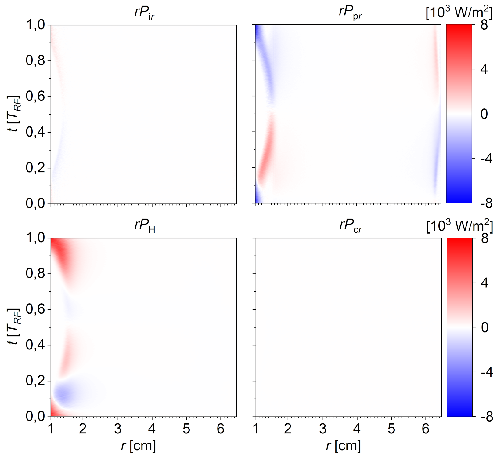
Figure 33: The radially weighted spatio-temporally resolved constituents from (60) of the power dissipation.

Figure 34: The spatio-temporally resolved Hall power and its constitutents.

Figure 35: Radially weighted ionization rate $rS_{\mathrm{e}}$ for the magnetized discharge.

Figure 36: Distribution of electrons in the $(v_{r},v_{\theta})$ plane of the velocity space sampled at different phases of the sheath evolution. The magenta circle indicates boundary of the inelastic energy range and corresponds to the $11.5$ eV argon excitation level.

Figure 37: Phase-resolved electron distribution in different directions for the magnetized case.Secondary electrons are not displayed.

REFERENCES

- (1) M. Lieberman and A. Lichtenberg, Principles of Plasma Discharges and Materials Processing. Wiley, 2nd ed. ed., 2005.
- (2) J. Thornton and A. Penfold, Thin Film Processes, ed L. Vossen and K. Kern. Academic, 1978.
- (3) B. Chapman, Glow Discharge Processes. Wiley, 1980.
- (4) I. Lin, D. Hinson, W. Class, and R. Sandstrom, “Low-energy high flux reactive ion etching by RF magnetron plasma,” Appl. Phys. Lett., vol. 44, p. 185, 1984.
- (5) D. Depla and S. Mahieu, Reactive Sputter Deposition. Springer, 2008.
- (6) D. Manos and D. Flamm, Plasma Etching – an Introduction. Academic, 1989.
- (7) G. Hagelaar and N. Oudini, “Plasma transport across magnetic field lines in low-temperature plasma sources,” Plasma Phys. Control. Fusion, vol. 53, p. 124032, 2011.
- (8) J. Thornton, “Planar magnetron sputtering,” Thin Solid Films, vol. 80, p. l, 1981.
- (9) A. Piel, Plasma Physics. Springer, 2017.
- (10) M. Kushner, “Modeling of magnetically enhanced capacitively coupled plasma sources: Ar discharges,” J. Appl. Phys., vol. 94, p. 1436, 2003.
- (11) S. Rossnagel, “Magnetron sputtering,” J. Vac. Sci. Technol. A, vol. 38, p. 060805, 2020.
- (12) J.-P. Boeuf and A. Smolyakov, “Preface to special topic: Modern issues and applications of E x B plasmas,” Phys. Plasmas, vol. 25, p. 061001, 2018.
- (13) I. Kaganovich et al., “Physics of E x B discharges relevant to plasma propulsion and similar technologies,” Phys. Plasmas, vol. 27, p. 120601, 2020.
- (14) A. Anders, “Localized heating of electrons in ionization zones: Going beyond the penning-thornton paradigm in magnetron sputtering,” Appl. Phys. Lett., vol. 105, p. 244104, 2014.
- (15) L. Tsendin, “Analytical approaches to glow discharge problems,” Plasma Sources Sci. Technol., vol. 20, p. 055011, 2011.
- (16) A. Kudryavtsev, A. Smirnov, and L. Tsendin, Physics of Glow Discharge (in Russian). Lan’, 2010.
- (17) V. Godyak, “The statistical heating of electrons by oscillating boundaries of the plasma,” Sov. Phys.-Tech. Phys., vol. 16, p. 1073, 1972.
- (18) M. Lieberman and V. Godyak, “From Fermi acceleration to collisionless discharge heating,” IEEE Trans. Plasma Sci., vol. 26, p. 955, 1998.
- (19) I. Kaganovich, V. Kolobov, and L. Tsendin, “Stochastic electron heating in bounded radio-frequency plasmas,” Appl. Phys. Lett., vol. 69, p. 3818, 1996.
- (20) T. Lafleur and P. Chabert, “Is collisionless heating in capacitively coupled plasmas really collisionless?,” Plasma Sources Sci. Technol., vol. 24, p. 044002, 2015.
- (21) G. Gozadinos, M. Turner, and D. Vender, “Collisionless electron heating by capacitive RF sheaths,” Phys. Rev. Lett., vol. 87, p. 135004, 2001.
- (22) J. Schulze, Z. Donkó, A. Derzsi, I. Korolov, and E. Schuengel, “The effect of ambipolar electric fields on the electron heating in capacitive RF plasmas,” Plasma Sources Sci. Technol., vol. 24, p. 015019, 2015.
- (23) M. Turner, “Collisionless heating in radio-frequency discharges: a review,” J. Phys. D: Appl. Phys., vol. 42, p. 194008, 2009.
- (24) T. Lafleur, P. Chabert, M. Turner, and J. Booth, “Equivalence of the hard-wall and kinetic-fluid models of collisionless electron heating in capacitively coupled discharges,” Plasma Sources Sci. Technol., vol. 23, p. 015016, 2014.
- (25) J. Schulze, Z. Donkó, T. Lafleur, S. Wilczek, and R. Brinkmann, “Spatio-temporal analysis of the electron power absorption in electropositive capacitive RF plasmas based on moments of the Boltzmann equation,” Plasma Sources Sci. Technol., vol. 27, p. 055010, 2018.
- (26) A. Sato and M. Lieberman, “Electron-beam probe measurements of electric fields in RF discharges,” J. Appl. Phys., vol. 68, p. 6117, 1990.
- (27) D. Vender and R. Boswell, “Electron-sheath interaction in capacitive radio-frequency plasmas,” J. Vac. Sci. Technol. A, vol. 10, p. 1331, 1992.
- (28) F. Tochikubo, T. Makabe, S. Kakuta, and A. Suzuki, “Study of the structure of radio frequency glow discharges in and by spatiotemporal optical emission spectroscopy,” J. Appl. Phys., vol. 71, p. 2143, 1992.
- (29) J. Schulze, Z. Donkó, B. Heil, D. Luggenhölscher, T. Mussenbrock, R. Brinkmann, and U. Czarnetzki, “Electric field reversals in the sheath region of capacitively coupled radio frequency discharges at different pressures,” J. Phys. D: Appl. Phys., vol. 41, p. 105214, 2008.
- (30) D. Eremin, T. Hemke, and T. Mussenbrock, “Nonlocal behavior of the excitation rate in highly collisional RF discharges,” Plasma Sources Sci. Technol., vol. 24, p. 044004, 2015.
- (31) U. Czarnetzki, T. Mussenbrock, and R. Brinkmann, “Self-excitation of the plasma series resonance in radio-frequency discharges: An analytical description,” Phys. Plasmas, vol. 13, p. 123503, 2006.
- (32) T. Mussenbrock, R. Brinkmann, M. Lieberman, A. Lichtenberg, and E. Kawamura, “Enhancement of Ohmic and stochastic heating by resonance effects in capacitive radio frequency discharges: a theoretical approach,” Phys. Rev. Lett., vol. 101, p. 085004, 2008.
- (33) M. Lieberman, A. Lichtenberg, E. Kawamura, T. Mussenbrock, and R. Brinkmann, “The effects of nonlinear series resonance on Ohmic and stochastic heating in capacitive discharges,” Phys. Plasmas, vol. 15, p. 063505, 2008.
- (34) Z. Donkó, J. Schulze, U. Czarnetzki, and D. Luggenhölscher, “Self-excited nonlinear plasma series resonance oscillations in geometrically symmetric capacitively coupled radio frequency discharges,” Appl. Phys. Lett., vol. 94, p. 131501, 2009.
- (35) S. Wilczek, J. Trieschmann, D. Eremin, R. Brinkmann, J. Schulze, E. Schüngel, A. Derzsi, I. Korolov, P. Hartmann, Z. Dónko, and T. Mussenbrock, “Kinetic interpretation of resonance phenomena in low pressure capacitively coupled radio frequency plasmas,” Phys. Plasmas, vol. 23, p. 063514, 2016.
- (36) S. Wilczek, J. Trieschmann, J. Schulze, Z. Donkó, R. Brinkmann, and T. Mussenbrock, “Disparity between current and voltage driven capacitively coupled radio frequency discharges,” Plasma Sources Sci. Technol., vol. 27, p. 125010, 2018.
- (37) P. Belenguer and J. Boeuf, “Transition between different regimes of RF glow discharges,” Phys. Rev. A, vol. 41, p. 4447, 1990.
- (38) V. Godyak, R. Piejak, and B. Alexandrovich, “Measurements of electron energy distribution in low-pressure RF discharges,” Plasma Sources Sci. Technol., vol. 1, p. 36, 1992.
- (39) R. Brinkmann, “Electron heating in capacitively coupled rf plasmas: a unified scenario,” Plasma Sources Sci. Technol., vol. 25, p. 25, 2016.
- (40) M. Lieberman, A. Lichtenberg, and S. Savas, “Model of magnetically enhanced, capacitive RF discharges,” IEEE Trans. Plasma Sci., vol. 1, p. 189, 1991.
- (41) Y. Okuno, Y. Ohtsu, and H. Fujita, “Electron acceleration resonant with sheath motion in a low-pressure radio frequency discharge,” Appl. Phys. Lett., vol. 64, p. 1623, 1994.
- (42) Q.-Z. Zhang, J.-Y. Sun, W.-Q. Lu, J. Schulze, Y.-Q. Guo, and Y.-N. Wang, “Resonant sheath heating in weakly magnetized capacitively coupled plasmas due to electron-cyclotron motion,” Phys. Rev. E, vol. 104, p. 045209, 2021.
- (43) S. Patil, S. Sharma, S. Sengupta, A. Sen, and I. Kaganovich, “Electron bounce-cyclotron resonance in capacitive discharges at low magnetic fields,” Phys. Rev. Research, vol. 4, p. 013059, 2022.
- (44) D. Hutchinson, M. Turner, R. Doyle, , and M. Hopkins, “The effects of a small transverse magnetic field upon a capacitively coupled RF discharge,” IEEE Trans. Plasma Sci., vol. 23, p. 636, 1995.
- (45) M. Turner, D. Hutchinson, R. Doyle, and M. Hopkins, “Heating mode transition induced by a magnetic field in a capacitive RF discharge,” Phys. Rev. Letters, vol. 76, p. 2069, 1996.
- (46) R. Krimke and H. Urbassek, “Influence of plasma extraction on a cylindrical low-pressure rf discharge: a PIC-MC study,” IEEE Trans. Plasma Sci., vol. 23, p. 103, 1995.
- (47) E. Barnat, P. Miller, and A. Paterson, “RF discharge under the influence of a transverse magnetic field,” Plasma Sources Sci. Technol., vol. 17, p. 045005, 2008.
- (48) S. You, T. Hai, M. Park, D. Kim, J. Kim, D. Seong, Y. Shin, S. Lee, G. Park, J. Lee, and H. Chang, “Role of transverse magnetic field in the capacitive discharge,” Thin Solid Films, vol. 519, p. 6981, 2011.
- (49) B. Zheng, K. Wang, T. Grotjohn, T. Schuelke, and Q. Fan, “Enhancement of Ohmic heating by Hall current in magnetized capacitively coupled discharges,” Plasma Sources Sci. Technol., vol. 28, p. 09LT03, 2019.
- (50) M. Oberberg, D. Engel, B. Berger, C. Wölfel, D. Eremin, J. Lunze, R. Brinkmann, P. Awakowicz, and J. Schulze, “Magnetic control of non-linear electron resonance heating in a capacitively coupled radio frequency discharge,” Plasma Sources Sci. Technol., vol. 28, p. 115021, 2019.
- (51) J. Joshi, S. Binwal, S. Karkari, and S. Kumar, “Electron series resonance in a magnetized 13.56 Mhz symmetric capacitive coupled discharge,” J. Appl. Phys., vol. 123, p. 113301, 2018.
- (52) M. Kushner, “Cylindrical magnetron discharges: II. the formation of dc bias in rf-driven discharge sources,” J. Appl. Phys., vol. 65, p. 3825, 1989.
- (53) R. Krimke, H. Urbassek, D. Korzec, and J. Engemann, “PIC/MC simulation of a strongly asymmetric low-pressure RF discharge,” J. Phys. D: Appl. Phys., vol. 27, p. 1653, 1994.
- (54) L. Wang, D.-Q. Wen, P. Hartmann, Z. Donkó, A. Derzsi, X.-F. Wang, Y.-H. Song, Y.-N. Wang, and J. Schulze, “Electron power absorption dynamics in magnetized capacitively coupled radio frequency oxygen discharges,” Plasma Sources Sci. Technol., vol. 29, p. 105004, 2020.
- (55) B. Zheng, Y. Fu, K. Wang, T. Schuelke, and Q. Fan, “Electron dynamics in radio frequency magnetron sputtering argon discharges with a dielectric target,” Plasma Sources Sci. Technol., vol. 30, p. 035019, 2021.
- (56) D. Eremin, B. Berger, D. Engel, J. Kallähn, K. Köhn, D. Krüger, L. Xu, M. Oberberg, C. Wölfel, J. Lunze, P. Awakowicz, J. Schulze, and R. Brinkmann, “Electron dynamics in planar radio frequency magnetron plasmas: II. Heating and energization mechanisms studied via a 2d3v particle-in-cell/Monte Carlo code,” Manuscript submitted for publication.
- (57) B. Berger, D. Eremin, M. Oberberg, D. Engel, C. Wölfel, Q.-Z. Zhang, P. Awakowicz, J. Lunze, R. Brinkmann, and J. Schulze, “Electron dynamics in planar radio frequency magnetron plasmas: III. Power absorption dynamics in capacitively coupled radio-frequency magnetrons with a conducting target,” Manuscript submitted for publication.
- (58) M. Panjan, “Self-organizing plasma behavior in rf magnetron sputtering discharges,” J. Appl. Phys., vol. 125, p. 203303, 2019.
- (59) R. Lucken, A. Tavant, A. Bourdon, M. Lieberman, and P. Chabert, “Saturation of the magnetic confinement in weakly ionized plasma,” Plasma Sources Sci. Technol., vol. 29, p. 065014, 2020.
- (60) L. Xu, D. Eremin, and R. P. Brinkmann, “Direct evidence of gradient drift instability being the origin of a rotating spoke in a crossed field plasma,” Plasma Sources Science and Technology, vol. 30, p. 075013, jul 2021.
- (61) M. Oberberg, J. Kallähn, P. Awakowicz, and J. Schulze, “Experimental investigations of the magnetic asymmetry effect in capacitively coupled radio frequency plasmas,” Plasma Sources Sci. Technol., vol. 27, p. 105018, 2018.
- (62) M. Oberberg, B. Berger, M. Buschheue, D. Engel, C. Woelfel, D. Eremin, J. Lunze, R. Brinkmann, P. Awakowicz, and J. Schulze, “The magnetic asymmetry effect in geometrically asymmetric capacitively coupled radio frequency discharges operated in Ar/O2,” Plasma Sources Sci. Technol., vol. 29, p. 075013, 2020.
- (63) J. Trieschmann, M. Shihab, D. Szeremley, A. Elgendy, S. Gallian, D. Eremin, R. Brinkmann, and T. Mussenbrock, “Ion energy distribution functions behind the sheaths of magnetized and non-magnetized radio frequency discharges,” J. Phys. D: Appl. Phys., vol. 46, p. 084016, 2013.
- (64) W. Qiu, Electron Series Resonance Plasma Discharges: Unmagnetized and Magnetized. PhD thesis, University of California, Berkeley, 2001.
- (65) J. Wesson, Tokamaks. Oxford University Press, 4th ed., 2011.
- (66) D. Eremin, “An energy- and charge-conserving electrostatic implicit particle-in-cell algorithm for simulations of collisional bounded plasmas,” J. Comput. Phys, vol. 452, p. 110934, 2022.
- (67) G. Chen, L. Chacón, and D. Barnes, “An energy- and charge-conserving, implicit, electrostatic particle-in-cell algorithm,” J. Comput. Phys., vol. 230, p. 7018, 2011.
- (68) D. Barnes and L. Chacón, “Finite spatial-grid effects in energy-conserving particle-in-cell algorithms,” Comput. Phys. Commun., vol. 258, p. 107560, 2021.
- (69) V. Vahedi and M. Surendra, “A Monte Carlo collision model for the particle-in-cell method: applications to argon and oxygen discharges,” Comput. Phys. Commun., vol. 87, p. 179, 1995.
- (70) P. Mertmann, D. Eremin, T. Mussenbrock, R. Brinkmann, and P. Awakowicz, “Fine-sorting one-dimensional particle-in-cell algorithm with Monte Carlo collisions on a graphics processing unit,” Comp. Phys. Comm., vol. 182, p. 2161, 2011.
- (71) A. Phelps and Z. Petrović, “Cold-cathode discharges and breakdown in argon: surface and gas phase production of secondary electrons,” Plasma Sources Sci. Technol., vol. 8, p. R21, 1999.
- (72) A. Phelps, “The application of scattering cross sections to ion flux models in discharge sheaths,” J. Appl. Phys., vol. 76, p. 747, 1994.
- (73) S. Markidis and G. Lapenta, “The energy conserving particle-in-cell method,” J. Comput. Phys., vol. 230, p. 7037, 2011.
- (74) M. Turner, A. Derzsi, Z. Donkó, D. Eremin, S. Kelly, T. Lafleur, and T. Mussenbrock, “Simulation benchmarks for low-pressure plasmas: Capacitive discharges,” Phys. Plasmas, vol. 20, p. 013507, 2013.
- (75) T. Charoy, J. Boeuf, A. Bourdon, J. Carlsson, P. Chabert, B. Cuenot, D. Eremin, L. Garrigues, K. Hara, I. Kaganovich, A. Powis, A. Smolyakov, D. Sydorenko, A. Tavant, O. Vermorel, and W. Villafana, “2d axial-azimuthal particle-in-cell benchmark for low-temperature partially magnetized plasmas,” Plasma Sources Sci. Technol., vol. 28, p. 105010, 2019.
- (76) W. Villafana, F. Petronio, A. Denig, M. Jimenez, D. Eremin, L. Garrigues, F. Taccogna, A. Alvarez-Laguna, J. Boeuf, A. Bourdon, P. Chabert, T. Charoy, B. Cuenot, K. Hara, F. Pechereau, A. Smolyakov, D. Sydorenko, A. Tavant, and O. Vermorel, “2d radial-azimuthal particle-in-cell benchmark for discharges,” Plasma Sources Sci. Technol., vol. 30, p. 075002, 2021.
- (77) S. Wilczek, J. Schulze, R. P. Brinkmann, Z. Donkó, J. Trieschmann, and T. Mussenbrock, “Electron dynamics in low pressure capacitively coupled radio frequency discharges,” Journal of Applied Physics, vol. 127, no. 18, p. 181101, 2020.
- (78) M. Surendra and M. Dalvie, “Moment analysis of RF parallel-plate-discharge simulations using the particle-in-cell with Monte Carlo collisions technique,” Phys. Rev. E, vol. 48, p. 3914, 1993.
- (79) R. Hazeltine and F. Waelbroeck, The Framework Of Plasma Physics. Westview Press, 2004.