Regularized Rényi divergence minimization through Bregman proximal gradient algorithms

Abstract

We study the variational inference problem of minimizing a regularized Rényi divergence over an exponential family, and propose a relaxed moment-matching algorithm, which includes a proximal-like step. Using the information-geometric link between Bregman divergences and the Kullback-Leibler divergence, this algorithm is shown to be equivalent to a Bregman proximal gradient algorithm. This novel perspective allows us to exploit the geometry of our approximate model while using stochastic black-box updates. We use this point of view to prove strong convergence guarantees including monotonic decrease of the objective, convergence to a stationary point or to the minimizer, and geometric convergence rates. These new theoretical insights lead to a versatile, robust, and competitive method, as illustrated by numerical experiments.

Keywords. Variational inference, Rényi divergence, Kullback-Leibler divergence, Exponential family, Bregman proximal gradient algorithm.

MSC2020 Subject Classification. 62F15, 62F30, 62B11, 90C26, 90C30.

1 Introduction

1.1 Variational inference

Probability distributions of interest in statistical problems are often intractable. In Bayesian statistics for instance, the targeted posterior distributions often cannot be obtained in closed-form due to intractable normalization constants. The construction of efficient approximating distributions is thus a core issue in these cases. Variational inference (VI) methods aim at finding good approximations by minimizing a divergence to the target over a family of parametric distributions [17, 101]. Such procedures can be summarized by the choice of approximating densities, the choice of divergence, and the algorithm used to solve the resulting optimization problem. As an example, the standard VI algorithm uses mean-field approximating densities and minimizes the exclusive Kullback-Leibler (KL) divergence [17]. Assuming that the complete conditionals of the true model are in an exponential family, the optimal mean-field approximation can then be found by a deterministic coordinate-ascent algorithm [52].

The research on VI methods has been very active in the last years (see [101] for a review). Majorization techniques have been proposed to cope with large scale models not satisfying conjugacy hypotheses [71, 102, 54]. Another approach in such challenging context is to run stochastic gradient descent, which leads to the so-called black-box VI methods [94, 66, 50, 7, 35]. Black-box methods allow a broad choice of divergence, like the $\alpha$-divergences [50, 35, 33] and Rényi divergences [89, 66], which are generalizations of the KL divergence depending on a scalar parameter $\alpha>0$. This parameter can be chosen in order to enforce a mode-seeking or a mass-covering behavior in the approximations. On the contrary, the exclusive KL divergence tends to produce approximations that under-estimate the variance of the target [76, 17].

VI algorithms have also benefited from advances in information geometry, a field that studies statistical models through a differential-geometric lens. Among other results from this field, it has been shown that the Fisher information matrix can play the role of a metric tensor such that the square of the induced Riemannian distance is locally equivalent to the KL divergence [2]. Another useful insight when exponential families are considered is the relation between the KL divergence, Bregman divergences, and dual geometry [4, 82]. These ideas can be leveraged by using the natural gradient [3], which amounts to a preconditioning of the standard gradient by the inverse Fisher information matrix. In the VI algorithms investigated in [53, 49, 52, 67], the standard gradient of the evidence lower bound is thus adjusted to take into account the Riemannian geometry of the approximating distributions, leading to simpler updates and improved behavior.

Despite those advances, there are still shortcomings in the development and understanding of VI algorithms, and as such, we identify below two main limitations.

First, to the best of our knowledge, there are still few links between black-box VI algorithms and natural gradient VI algorithms in the literature. On the one hand, the former methods allow to tackle a broad range of targets using various divergence measures but are usually restricted to the use of standard stochastic gradients. On the other hand, the latter methods use the more efficient and robust natural gradients, but are often limited to certain class of divergence, target, and approximating family. In this direction, let us however mention that information-geometric procedures have been deployed along black-box updates in [59, 58, 56], but these works remain restricted to the minimization of the exclusive KL divergence. One can also mention [90] where the minimization of an $\alpha$-divergence over a mean-field family is studied using the Fisher Riemannian geometry.

Second, convergence studies of VI schemes are mostly empirical for black-box VI schemes [94, 66, 50, 7, 35], and the same arises for schemes based on natural gradients [53, 49, 52, 67]. Indeed, the considered optimization problems are non-convex, making the algorithms hard to analyze (see however [33] for a study in a convex setting). This is in stark contrast with MCMC methods, which can be used alternatively to VI, or optimization procedures, upon which many VI methods are based. MCMC methods based on Langevin diffusion are guaranteed to asymptotically produce samples from the target but also benefit from non-asymptotic convergence guarantees [97, 38, 69]. These results hold under log-concavity assumptions on the target and leverage the technology of Wasserstein gradient flows [5]. Recent works in VI have employed such techniques to prove convergence to the minimizer of the exclusive KL divergence, in the case of a mean-field approximating family [99] or a Gaussian approximating family [65], under the same type of hypotheses. Note that both aforementioned schemes require the gradients of the logarithm of the target to be implemented exactly, which may be costly or even impossible in a black-box setting [88]. On the other hand, convergence results in the optimization literature include monotonic decrease of the objective, which has been proven for some VI schemes, but also convergence to a minimizer, or a stationary point for non-convex problems, and rates of convergence, even for composite objectives with one non-differentiable term [11].

1.2 Contributions and outline

In this paper, we propose a novel VI algorithm that links black-box VI methods and VI methods based on natural gradients, while benefiting from solid convergence guarantees. Our algorithm minimizes a versatile composite objective, which is the sum of a Rényi divergence between the target and an exponential family, and a possible regularization term.

In order to solve the minimization problem, we introduce the so-called proximal relaxed moment-matching algorithm, whose iterations are composed of a relaxed moment-matching step, followed by a proximal-like step. A sampling-based implementation using only evaluations of the target unnormalized density is also provided to cover the black-box setting. The convergence of our new algorithm is then studied using the theory of Bregman proximal gradient algorithms. In particular, it exploits an equivalence relationship between Bregman divergences and the KL divergence arising when doing VI within the space of exponential families.

Bregman proximal gradient algorithms [12, 13, 93, 79, 80] are recent optimization methods arising from the generalization of the powerful proximal minimization schemes from the Euclidean setting [28]. Bregman-based algorithms allow to choose a Bregman divergence that tailors the intrinsic geometry of an optimization problem, more suitably than the standard Euclidean one [13, 93]. Note that stochastic methods have also been generalized in this fashion [47, 98]. Also related are proximal methods on perspective functions [29, 40], where divergences (typically, $\phi$-divergence) are directly processed through their proximity operator on the Euclidean metric.

We show in this paper that the connection between VI algorithms and proximal optimization algorithms written in Bregman geometry yields many theoretical and practical insights. To summarize, our main contributions are the following:

• We propose a deterministic VI algorithm for an exponential approximating family. We show that our method can be written as a Bregman proximal gradient algorithm whose Bregman divergence is induced by the KL divergence, and exploits per se the geometry of the approximating family. We propose a stochastic implementation for our method. We show that it can be seen as a stochastic Bregman proximal gradient algorithm in the same geometry, thus bridging the gap between information-geometric and black-box VI methods.

• Our deterministic algorithm is shown to achieve a monotonic decrease of the composite objective, with its fixed points being stationary points of the objective function. Convergence to these stationary points is established. We show that this scheme achieves a geometric convergence rate to the global minimizer, guaranteed to exist and to be unique, in the case when the Rényi divergence identifies with the inclusive KL divergence or when the target belongs to the considered approximating family. We also show that the stochastic implementation recovers the deterministic one in the large sample limit, thus demonstrating the well-posedness of the proposed sampling-based implementation.

• We explain through a simple counter-example how the convergence of equivalent schemes written in the Euclidean geometry may fail. This theoretical insight is backed by numerical studies highlighting the superior performance and robustness of our scheme over its Euclidean counterpart.

• Our algorithm generalizes many existing moment-matching algorithms. We show through numerical experiments in the Gaussian case how our additional parameters allow to create mass-covering or mode-seeking approximations and compensate high approximation errors.

• Our framework allows a possibly non-smooth regularization term that is handled in our algorithm through a proximal update. This allows in particular to use our algorithms to compute generalized information projections. We explicit the proximal operators of two regularizers that promote the good conditioning of the covariance matrix or the sparsity of the means of the approximating densities.

The paper is organized as follows. In Section 2, we recall basic facts about Rényi divergences and exponential families, before presenting the optimization problem we propose to solve. Then, in Section 3, we outline our algorithm, before providing an alternative black-box implementation for it. In Section 4, we show how these algorithms can be interpreted as Bregman proximal gradient algorithms in the geometry induced by the KL divergence, and state our working assumptions. Theoretical analysis is provided in Section 5. Finally, numerical experiments with Gaussian proposals are presented in Section 6. We discuss our results and possible future research lines in Section 7.

The supplementary material contains four appendices. The proofs of our results are deferred to Appendices A and B, while the computations of the proximal operators are conducted in Appendix C. Additional numerical experiments are presented in Appendix D.

1.3 Notation

The discrete set $\{n_{1},n_{1}+1,\ldots,n_{2}\}$ defined for $n_{1},n_{2}\in\mathbb{N}$, $n_{1}<n_{2}$ is denoted by $\llbracket n_{1},n_{2}\rrbracket$. Throughout this work, $\mathcal{H}$ is a real Hilbert space of finite dimension $n$ with scalar product $\langle\cdot,\cdot\rangle$ and norm $\|\cdot\|$. We denote by $B(\theta,R)$ the closed ball centered at $\theta\in\mathcal{H}$ with radius $R>0$. The interior of a set $C$ is denoted by $\operatorname*{int}C$. The set of non-negative real numbers if denotes by $\mathbb{R}_{+}$ and the set of positive real numbers by $\mathbb{R}_{++}$. Similarly, we denote by $\mathbb{R}_{-}$ and $\mathbb{R}_{--}$ the sets of non-positive and negative real numbers, respectively. Consider the set of matrices of $\mathbb{R}^{d\times d}$. Then, the set of symmetric matrices is denoted by $\mathcal{S}^{d}$, the set of positive semidefinite matrices is denoted by $\mathcal{S}_{+}^{d}$, and the set of positive definite matrices is denoted by $\mathcal{S}_{++}^{d}$. The identity matrix is denoted by $I$, $\det(\cdot)$ denotes the determinant operator on matrices and $\|\cdot\|_{F}$ the Frobenius norm. We use Landau’s notation, i.e. for some functions $f,g:\mathcal{H}\rightarrow\mathbb{R}$, we write $f(\upsilon)=o(g(\upsilon))$ if $f$ is such that, for any $\epsilon>0$, there exists $\upsilon_{0}$ with $\|\upsilon_{0}\|$ small enough such that $|f(\upsilon)|\leq\epsilon|g(\upsilon)|$ for any $\upsilon\in B(0,\|\upsilon_{0}\|)$. Convex analysis notations are those from [11]. In particular, we denote by $\Gamma_{0}(\mathcal{H})$ the set of proper convex lower-semicontinuous functions from $\mathcal{H}$ to $\mathbb{R}\cup\{+\infty\}$. The domain of a function $f:\mathcal{H}\rightarrow[-\infty,+\infty]$ is $\operatorname*{dom}f:=\{\theta\in\mathcal{H},\,f(\theta)<+\infty\}.$ The indicator function function $\iota_{C}$ of a set $C\subset\mathcal{H}$ is defined for every $\theta\in\mathcal{H}$ by

$$\iota_{C}(\theta)=\begin{cases}0&\text{ if }\theta\in C,\\ +\infty&\text{ else}.\end{cases}$$

We adopt measure theory notations following [26]. In particular, the Borel algebra of a set $\mathcal{X}$ is denoted by $\mathcal{B}(\mathcal{X})$. $\mathcal{M}(\mathcal{X})$ is the set of measures on $(\mathcal{X},\mathcal{B}(\mathcal{X}))$, and $\mathcal{P}(\mathcal{X})$ is the set of probability measures on $(\mathcal{X},\mathcal{B}(\mathcal{X}))$. Given $m_{1},m_{2}\in\mathcal{M}(\mathcal{X})$, we write $m_{1}\ll m_{2}$ when $m_{1}$ is absolutely continuous with respect to $m_{2}$. For a given $m\in\mathcal{M}(\mathcal{X})$ and a measurable function $h:\mathcal{X}\rightarrow\mathcal{H}$, we denote by $m(h)$ the vector of $\mathcal{H}$ defined by $(m(h))_{i}=\int_{\mathcal{X}}h_{i}(x)m(dx)$ for $i\in\llbracket 1,n\rrbracket$. Finally, $\mathcal{N}(\cdot\,;\mu,\Sigma)$ denotes the density of a Gaussian probability measure with mean $\mu\in\mathbb{R}^{d}$ and covariance $\Sigma\in\mathcal{S}_{++}^{d}$.

2 Problem of interest

We propose to reformulate the problem of approximating a target $\pi$ by a parametric distribution $q_{\theta}$ as a variational minimization problem. In this context, the optimal parameters $\theta$ are defined to minimize a divergence to the target. Specifically, we focus here on the case when $q_{\theta}$ lies in an exponential family, and we propose to optimize its parameters $\theta$ through the minimization of a Rényi divergence between $\pi$ and $q_{\theta}$ with a regularization term. In this section, we first recall important definitions regarding Rényi divergences (including the Kullback-Leibler divergence as a special case) and exponential families. We then introduce our variational inference (VI) problem.

Let $(\mathcal{X},\mathcal{B}(\mathcal{X}))$ be a measurable space. Let us consider a measure $\nu\in\mathcal{M}(\mathcal{X})$, with the sets $\mathcal{M}(\mathcal{X},\nu):=\{m\in\mathcal{M}(\mathcal{X}),\,m\ll\nu\}$ and $\mathcal{P}(\mathcal{X},\nu):=\{p\in\mathcal{P}(\mathcal{X}),\,p\ll\nu\}$. We are interested in approximating the target probability distribution $\pi\in\mathcal{P}(\mathcal{X},\nu)$.

2.1 Rényi and Kullback-Leibler divergences

Rényi divergences [89] and Kullback-Leibler (KL) divergence [64] are widely used in statistics as discrepancy measures between probability distributions. To define them, let us consider two probability densities $p_{1},p_{2}\in\mathcal{P}(\mathcal{X},\nu)$. We can then define the Rényi and KL divergences between $p_{1}$ and $p_{2}$ as follows.

Definition 1.

The Rényi divergence with parameter $\alpha>0$, $\alpha\neq 1$, between $p_{1}$ and $p_{2}$ is defined by

$$RD_{\alpha}(p_{1},p_{2})=\frac{1}{\alpha-1}\log\left(\int p_{1}(x)^{\alpha}p_{2}(x)^{1-\alpha}\nu(dx)\right).$$

When the above integral is not well-defined, then $RD_{\alpha}(p_{1},p_{2})=+\infty$.

Definition 2.

The KL divergence between $p_{1}$ and $p_{2}$ is defined by

$$KL(p_{1},p_{2})=\int\log\left(\frac{p_{1}(x)}{p_{2}(x)}\right)p_{1}(x)\nu(dx).$$

When the above integral is not well-defined, then $KL(p_{1},p_{2})=+\infty$.

The KL divergence is a limiting case of Rényi divergence [95], since

$$\lim_{\alpha\rightarrow 1,\,\alpha\leq 1}RD_{\alpha}(p_{1},p_{2})=KL(p_{1},p_{2}).$$

Note that the same result also holds by taking the limit from above $\alpha=1$ under some additional conditions [95].

Let us recall the important following property, that explains the term divergence:

Proposition 1 ([95]).

For any $\alpha>0$, $\alpha\neq 1$,

$$RD_{\alpha}(p_{1},p_{2})\geq 0,\text{ and }RD_{\alpha}(p_{1},p_{2})=0\text{ if and only if }p_{1}=p_{2}.$$

Moreover,

$$KL(p_{1},p_{2})\geq 0,\text{ and }KL(p_{1},p_{2})=0\text{ if and only if }p_{1}=p_{2}.$$

2.2 Exponential families

In this work, we propose to approximate the target $\pi\in\mathcal{P}(\mathcal{X},\nu)$ by a parametric distribution taken from an exponential family [19, 9].

Definition 3.

Let $\Gamma:\mathcal{X}\rightarrow\mathcal{H}$ be a Borel-measurable function. The exponential family with base measure $\nu$ and sufficient statistics $\Gamma$ is the family $\mathcal{Q}=\{q_{\theta}\in\mathcal{P}(\mathcal{X},\nu),\,\theta\in\Theta\}$ such that

$$q_{\theta}(x)=\exp\left(\langle\theta,\Gamma(x)\rangle-A(\theta)\right),\,\forall x\in\mathcal{X},$$ (1)

with $A$ being the log-partition function, such that $\Theta=\operatorname*{dom}A\subset\mathcal{H}$, and which reads:

$$A(\theta)=\log\left(\int\exp\left(\langle\theta,\Gamma(x)\rangle\right)\nu(dx)\right),\,\forall\theta\in\Theta.$$ (2)

In the following, for the sake of conciseness, we will say that some family $\mathcal{Q}$ is an exponential family, without stating explicitly the base measure and the sufficient statistics $\mathcal{Q}$ is associated to.

Remark 1.

We work here with parameters in the finite-dimensional Hilbert space $\mathcal{H}$, which is slightly more general than considering parameters in $\mathbb{R}^{n}$. This allows to consider vectors, matrices, or Cartesian products in a unified way. In particular, when symmetric matrices are considered, we work directly with $\mathcal{S}^{d}$ rather than with its vectorized counterpart $\mathbb{R}^{d(d+1)/2}$.

The goal of our approximation method is thus to find $\theta\in\Theta$ such that $q_{\theta}$ is an optimal approximation of $\pi$, in a sense that remains to be precised. Before going further, let us provide an important example of an exponential family.

Example 1.

Let $d\geq 1$. Consider the family of Gaussian distributions with mean $\mu\in\mathbb{R}^{d}$ and covariance $\Sigma\in\mathcal{S}^{d}_{++}$. This is an exponential family [9], with sufficient statistics $\Gamma:x\longmapsto\left(x,xx^{\top}\right)^{\top}$ and Lebesgue base measure that we denote by $\mathcal{G}$ in the following. Its corresponding parameters are $\theta=(\theta_{1},\theta_{2})^{\top}$ with $\theta_{1}=\Sigma^{-1}\mu$, and $\theta_{2}=-\frac{1}{2}\Sigma^{-1}$, while $A(\theta)=\frac{d}{2}\log(2\pi)-\frac{1}{4}\theta_{1}^{\top}\theta_{2}^{-1}\theta_{1}-\frac{1}{2}\operatorname*{log\,det}(-2\theta_{2})$. The domain of $A$ is $\Theta=\mathbb{R}^{d}\times\left(-\mathcal{S}^{d}_{++}\right)$, which is included in $\mathcal{H}=\mathbb{R}^{d}\times\mathcal{S}^{d}$. The scalar product of $\mathcal{H}$ is taken as the sum of the scalar product of $\mathbb{R}^{d}$ and the one of $\mathcal{S}^{d}$. Under such parametrization, for any $x\in\mathbb{R}^{d}$ and $\theta\in\Theta$,

$$q_{\theta}(x) =\exp\left(\langle\theta_{1},x\rangle+\langle\theta_{2},xx^{\top}\rangle-A(\theta)\right)$$

$$=\exp\left(\mu^{\top}\Sigma^{-1}x-\frac{1}{2}x^{\top}\Sigma^{-1}x-\frac{1}{2}\mu^{\top}\Sigma^{-1}\mu-\frac{1}{2}\log((2\pi)^{d}\det(\Sigma))\right)$$

$$=\mathcal{N}(x;\mu,\Sigma).$$

Exponential families recover many other continuous distributions, such as the inverse Gaussian and Wishart distributions, among others. Discrete distributions can also be put under the form (1) when $\nu$ is chosen as a discrete measure. Exponential families benefit from a rich geometric structure [2, 82] and have been used as approximating families in many contexts such as VI algorithms [49, 52, 17, 67], expectation-propagation schemes [91], or adaptive importance sampling (AIS) procedures [1].

2.3 Proposed approximation approach

We seek to approximate $\pi$ by a parametric distribution $q_{\theta}$ from an exponential family $\mathcal{Q}$ with base measure $\nu$, such that the domain $\Theta\subset\mathcal{H}$ is non-empty. To measure the quality of our approximations, we define the following family of functions $f_{\pi}^{(\alpha)}$ for $\alpha>0$:

$$f_{\pi}^{(\alpha)}(\theta):=\begin{cases}RD_{\alpha}(\pi,q_{\theta}),&\text{ if }\alpha\neq 1,\\ KL(\pi,q_{\theta}),&\text{ if }\alpha=1,\end{cases}\,\forall\theta\in\Theta.$$ (3)

Consider now a regularizing term $r$, which promotes desirable properties on the sought parameters $\theta$. We now define our objective function for some $\alpha>0$:

$$F_{\pi}^{(\alpha)}(\theta):=f_{\pi}^{(\alpha)}(\theta)+r(\theta),\,\forall\theta\in\Theta.$$ (4)

We propose to resolve our approximation problem by minimizing (4) over an exponential family $\mathcal{Q}$, i.e., by considering the following optimization problem:

$$\operatorname*{minimize}_{\theta\in\Theta}\,F_{\pi}^{(\alpha)}(\theta). P_{\pi}^{(\alpha)}$$ ()

Problem ($P_{\pi}^{(\alpha)}$) consists in minimizing $F_{\pi}^{(\alpha)}$, which is the sum of the Rényi divergence $RD_{\alpha}(\pi,\cdot)$ and a regularizing function $r$. This allows to capture or generalize many settings.

Minimizing the KL divergence leads to a particular behavior that may be undesirable in practice. For instance, minimizing $KL(\pi,\cdot)$ induces a mass-covering behavior while minimizing $KL(\cdot,\pi)$ induces a mode-fitting behavior [76, 17]. In contrast, working with a Rényi divergence as a discrepancy measure allows to generalize KL divergence [63, 91, 37, 24], recovered when $\alpha=1$ while allowing to choose the right value of $\alpha$ [66], hence fine-tuning the algorithm’s behavior for the application at hand. Moreover, the Rényi divergence with parameter $\alpha$ can be monotonically transformed [95] into the corresponding $\alpha$-divergence [75, 50, 33], including in particular the Hellinger distance [23] and the $\chi^{2}$ divergence [35, 1].

Adding a regularization term gives even more possibilities. When $r$ is null or an indicator function, then Problem ($P_{\pi}^{(\alpha)}$) relates to the computation of the so-called reverse information projection [31, 39, 32] when $\alpha=1$, which has later been generalized in [68] for $\alpha\neq 1$. A similar setting is used in sparse precision matrix estimation, relying on the KL divergence and a sparsity-inducing regularizer [100, 8]. The problem of computing Bayesian core-sets has also been formulated as a KL minimization problem over a set of sparse parameters [22]. Let us also cite [92], that performs VI with an added graph regularization term, used to enforce special geometric structure. Finally, the minimization of problems composed of a divergence and an additional term is at the core of the generalized view on variational inference proposed in [60].

3 A proximal relaxed moment-matching algorithm

In this section, we detail our proposed algorithm and its behavior, and discuss its connections with existing works. Our algorithm solves Problem ($P_{\pi}^{(\alpha)}$) by adapting the parameters $\theta$ iteratively. Each iteration is composed of two steps: (i) a relaxed moment-matching step, and (ii) a proximal step, both described in Section 3.1. Then, we provide a black-box implementation of our method based on non-linear importance sampling in Section 3.2. Finally, we discuss in Section 3.3 how our method generalizes existing moment-matching algorithms.

3.1 A proximal relaxed moment-matching algorithm

In order to state our algorithm, we first introduce the notion of geometric average between our target $\pi$ and the parametric density $q_{\theta}$.

Definition 4.

Consider $\theta\in\Theta$ and $\alpha>0$. We introduce, whenever it is well-defined, the geometric average with parameter $\alpha$ between $\pi$ and $q_{\theta}$, denoted by $\pi_{\theta}^{(\alpha)}$, which is the probability distribution of $\mathcal{P}(\mathcal{X},\nu)$ defined by

$$\pi_{\theta}^{(\alpha)}(x)=\frac{1}{\int\pi(y)^{\alpha}q_{\theta}(y)^{1-\alpha}\nu(dy)}\left(\pi(x)^{\alpha}q_{\theta}(x)^{1-\alpha}\right),\,\forall x\in\mathcal{X}.$$ (5)

Probability densities akin to $\pi_{\theta}^{(\alpha)}$ have been used for instance in annealing importance sampling [81], in sequential Monte-Carlo schemes [77], or in adaptive importance sampling [20]. The integral in (5) is well-defined if $\alpha\leq 1$ and the supports of $\pi$ and $q_{\theta}$ have non-empty intersection. Since $\pi$ and every $q_{\theta}\in\mathcal{Q}$ are absolutely continuous with respect to $\nu$, and $q_{\theta}(x)>0$ for every $x\in\mathcal{X}$, the latter condition is always satisfied within the setting of our study.

Remark 2.

If one does not have access to $\pi$ but only to an unnormalized density $\tilde{\pi}$ such that $\pi(x)=\frac{1}{Z_{\pi}}\tilde{\pi}(x)$, the geometric average between $\pi$ and $q_{\theta}$ can be still computed using

$$\pi_{\theta}^{(\alpha)}(x)=\frac{1}{\int\tilde{\pi}(y)^{\alpha}q_{\theta}(y)^{1-\alpha}\nu(dy)}\left(\tilde{\pi}(x)^{\alpha}q_{\theta}(x)^{1-\alpha}\right),\,\forall x\in\mathcal{X}.$$

We are now ready to introduce our proximal relaxed moment-matching algorithm, described in Algorithm 1. At iteration $k$, the first step, Eq. (6) can be viewed as a relaxed form of a moment-matching step, with relaxation step-size $\tau_{k+1}$ chosen such that $\tau_{k+1}\in(0,1]$. The parameter $\alpha$ arises from the Rényi divergence $f_{\pi}^{(\alpha)}$. The second step, Eq. (7), is a so-called proximal step on the regularization term $r$ (see Section 4.1) that involves again the step-size $\tau_{k+1}$.

Choose the step-sizes $\{\tau_{k}\}_{k\in\mathbb{N}}$, such that $\tau_{k}\in(0,1]$ for any $k\in\mathbb{N}$.

Set the Rényi parameter $\alpha>0$.

Initialize the algorithm with $\theta_{0}\in\operatorname*{int}\Theta$.

for $k=0,...$ do

       Compute $\theta_{k+\frac{1}{2}}$ such that

$$q_{\theta_{k+\frac{1}{2}}}(\Gamma)=\tau_{k+1}\pi_{\theta_{k}}^{(\alpha)}(\Gamma)+(1-\tau_{k+1})q_{\theta_{k}}(\Gamma).$$ (6)

       Update $\theta_{k+1}$ following

$$\theta_{k+1}=\operatorname*{arg\,min}_{\theta^{\prime}\in\Theta}\left(r(\theta^{\prime})+\frac{1}{\tau_{k+1}}KL(q_{\theta_{k+\frac{1}{2}}},q_{\theta^{\prime}})\right).$$ (7)

end for

Algorithm 1 Proposed proximal relaxed matching algorithm

The following example explicits the relaxed moment-matching step of Algorithm 1 when the exponential family is Gaussian.

Example 2.

In the case when $\mathcal{Q}=\mathcal{G}$, the first and second order moments $q_{\theta}(\Gamma)=(q_{\theta}(x),q_{\theta}(xx^{\top}))^{\top}$ are the sufficient statistics of the distribution. The update (6) reads in this case

$$\begin{cases}q_{\theta_{k+\frac{1}{2}}}(x)&=\tau_{k+1}\pi_{\theta_{k}}^{(\alpha)}(x)+(1-\tau_{k+1})q_{\theta_{k}}(x),\\ q_{\theta_{k+\frac{1}{2}}}(xx^{\top})&=\tau_{k+1}\pi_{\theta_{k}}^{(\alpha)}(xx^{\top})+(1-\tau_{k+1})q_{\theta_{k}}(xx^{\top}).\end{cases}$$ (8)

This shows that (6) consists in matching the first and second order moments of the new distribution $q_{\theta_{k+\frac{1}{2}}}$ with a convex combination between the moments of $\pi_{\theta_{k}}^{(\alpha)}$ and those of the previous distribution $q_{\theta_{k}}$. We recall that, for $q_{\theta}\in\mathcal{G}$, $q_{\theta}(x)=\mu$ and $q_{\theta}(xx^{\top})=\Sigma+\mu\mu^{\top}$. Thus, we can further write that (8) is equivalent to

$$\begin{cases}\mu_{k+\frac{1}{2}}&=\tau_{k+1}\pi_{\theta_{k}}^{(\alpha)}(x)+(1-\tau_{k+1})\mu_{k},\\ \Sigma_{k+\frac{1}{2}}&=\tau_{k+1}\pi_{\theta_{k}}^{(\alpha)}(xx^{\top})+(1-\tau_{k+1})\left(\Sigma_{k}+\mu_{k}\mu_{k}^{\top}\right)-\mu_{k+\frac{1}{2}}\mu_{k+\frac{1}{2}}^{\top}.\end{cases}$$

We now give an example in order to illustrate the second step of Algorithm 1. This example is rather general and links Eq. (7) with reverse information projections [31, 39, 32]. A list of comprehensive examples of this step is provided in Appendix C.

Example 3.

The proximal step (7) encompasses the notion of projection if the function $r$ is the indicator $\iota_{C}$ of a non-empty closed convex set $C\subset\mathcal{H}$ [11, Example 12.25]. We obtain in this case

$$\theta_{k+1}=\operatorname*{arg\,min}_{\theta^{\prime}\in\Theta\cap C}KL(q_{\theta_{k+\frac{1}{2}}},q_{\theta^{\prime}}).$$

We recognize that in this case, (7) is the reversed information projection of $q_{\theta_{k+\frac{1}{2}}}$ on the set $\{q_{\theta}\in\mathcal{Q},\,\theta\in C\cap\Theta\}$, as described in [32, Section 3] for instance.

3.2 A black-box implementation based on non-linear importance sampling

Implementing directly Algorithm 1 might not be possible in practice. In many situations, $\pi_{\theta}^{(\alpha)}(\Gamma)$ cannot be expressed analytically, and must be approximated. We thus propose a stochastic implementation of Algorithm 1 based on non-linear importance sampling. This new scheme only requires that samples distributed following $q_{\theta}$ are available for any $\theta\in\Theta$, and that an unnormalized version of $\pi$ can be evaluated. This means that there exists $\tilde{\pi}\in\mathcal{M}(\mathcal{X},\nu)$ and $Z_{\pi}>0$ such that for any $x\in\mathcal{X}$, $\pi(x)=\frac{1}{Z_{\pi}}\tilde{\pi}(x)$ with $\tilde{\pi}(x)$ being easy to compute.

This setting is standard in importance sampling as well as in black-box VI [85] for instance. The proposed stochastic form of Algorithm 1 is motivated by the following alternative form of $\pi_{\theta}^{(\alpha)}(\Gamma)$:

$$\pi_{\theta}^{(\alpha)}(\Gamma)=\frac{1}{\int\left(\frac{\tilde{\pi}(y)}{q_{\theta}(y)}\right)^{\alpha}q_{\theta}(y)\nu(dy)}\int\left(\frac{\tilde{\pi}(x)}{q_{\theta}(x)}\right)^{\alpha}\Gamma(x)q_{\theta}(x)\nu(dx).$$ (9)

We see here that both integrals in Eq. (9) are expectations with respect to $q_{\theta}$, with the ratios $\left(\frac{\tilde{\pi}(x)}{q_{\theta}(x)}\right)^{\alpha}$ evoking exponentiated importance weights. Therefore, our approximate implementation of Algorithm 1 consists in approximating these integrals with weighted samples from $q_{\theta}$, which yields Algorithm 2.

Choose the step-sizes $\{\tau_{k}\}_{k\in\mathbb{N}}$, such that $\tau_{k}\in(0,1]$ for any $k\in\mathbb{N}$.

Choose the sample sizes $\{N_{k}\}_{k\in\mathbb{N}}$, such that $N_{k}\in\mathbb{N}\setminus\{0\}$ for any $k\in\mathbb{N}$.

Set the Rényi parameter $\alpha>0$.

Initialize the algorithm with $\theta_{0}\in\operatorname*{int}\Theta$.

for $k=0,...$ do

       Sample $x_{l}\sim q_{\theta_{k}}$ for $l\in\llbracket 1,N_{k+1}\rrbracket$.

       For every $l\in\llbracket 1,N_{k+1}\rrbracket$, compute the non-linear importance weight $w_{l}^{(\alpha)}$ and their normalized counterpart $\bar{w}_{l}^{(\alpha)}$ through

$$w_{l}^{(\alpha)}=\left(\frac{\tilde{\pi}(x_{l})}{q_{\theta_{k}}(x_{l})}\right)^{\alpha},\quad\bar{w}_{l}^{(\alpha)}=\frac{w_{l}^{(\alpha)}}{\sum_{l=1}^{N_{k+1}}w_{l}^{(\alpha)}}.$$ (10)

       Compute $\theta_{k+\frac{1}{2}}$ such that

$$q_{\theta_{k+\frac{1}{2}}}(\Gamma)=\tau_{k+1}\left(\sum_{l=1}^{N_{k+1}}\bar{w}_{l}^{(\alpha)}\Gamma(x_{l})\right)+(1-\tau_{k+1})q_{\theta_{k}}(\Gamma).$$ (11)

       Update $\theta_{k+1}$ following

$$\theta_{k+1}=\operatorname*{arg\,min}_{\theta^{\prime}\in\Theta}\left(r(\theta^{\prime})+\frac{1}{\tau_{k+1}}KL(q_{\theta_{k+\frac{1}{2}}},q_{\theta^{\prime}})\right).$$ (12)

end for

Algorithm 2 Proposed Monte Carlo proximal relaxed moment-matching algorithm

Algorithms 1 and 2 are both written assuming that the proximal step can be computed exactly. Examples of such computations are provided in Appendix C. However, it may not be the case, depending on $r$ and $\mathcal{Q}$. Still, the minimization step in (12) is easier to solve than Problem ($P_{\pi}^{(\alpha)}$) since we deal with the KL divergence rather than the Rényi divergence (see Proposition 9 to see why this case leads to better properties) and the target is now $q_{\theta_{k+\frac{1}{2}}}\in\mathcal{Q}$. This property can be exploited by using specialized optimization subroutines to approximate this step. Specific cases have been investigated in the literature. For instance, the proximal algorithm proposed in [15] can be used in the case of Gaussian densities with fixed mean. A graphical lasso solver such as [100, 8] can also be employed for computation of this step for Gaussian densities with fixed mean and $\ell_{1}$ regularizer. When $r=\iota_{C}$, the substep of Eq. (12) reduces to a reversed information projection, as discussed in Example 3. Note that in this case, Problem ($P_{\pi}^{(\alpha)}$) reads

$$\operatorname*{minimize}_{\theta\in\Theta\cap C}RD_{\alpha}(\pi,q_{\theta}).$$ (13)

When $\alpha\in(0,1)$, the skew-symetry property of the Rényi divergence [95, Proposition 2] makes this problem equivalent to the following one:

$$\operatorname*{minimize}_{\theta\in\Theta\cap C}RD_{\alpha}(q_{\theta},\pi).$$ (14)

This shows that Algorithm 1 allows to compute the Rényi information projections described in Eq. (13)-(14) using a sequence of reversed information projections, that may be more easily available. Rényi information projections have been studied for instance in [68], where possible applications are discussed.

3.3 Comparison with existing moment-matching algorithms

Let us now discuss the main features of our algorithms, and their positioning with respect to existing moment-matching algorithms. First, note that a strict moment-matching update of $\theta_{k+1}$,

$$q_{\theta_{k+1}}(\Gamma)=\pi(\Gamma),$$ (15)

is recovered in Algorithm 1 when $\tau_{k+1}=1$, $\alpha=1$ and $r\equiv 0$. Therefore, each update of Algorithm 1 can be viewed as a generalized version of the strict moment-matching update of Eq. (15) with supplementary degrees of freedom, hence its name.

Many algorithms in statistics resort to moment-matching updates. In AIS, the AMIS scheme [30, 70] and the M-PMC scheme [24] rely on such updates. The idea of moment-matching updates with $\tau>0$ as in (6) can also be found in many contexts, such as VI [58], covariance learning in adaptive importance sampling [41] or in the cross-entropy method [63], although $\pi$ is not used directly in the latter. However, all the aforementioned works consider KL-based updates, that is with $\alpha=1$ and no regularization term (i.e., $r\equiv 0$).

Moment-matching updates are often approximated through AIS, as we do in Algorithm 2. Importance sampling estimation of $\pi(\Gamma)$ or $\pi_{\theta}^{(\alpha)}(\Gamma)$ is for instance used in the AMIS scheme of [30, 70, 42] for adaptive importance sampling, where proposals are constructed by matching the moments of the target. AMIS is recovered when $\alpha=1,\tau_{k}\equiv 1$ and $r\equiv 0$. However, note that in AMIS, all the past samples are used at each iteration and re-weighted (interpreting that samples are simulated in a multiple IS setting [43]), which is not the case here. In that respect, the APIS algorithm [72] bears some similarity, since it performs adaptation via moment matching with only the samples at each given iteration. Let us also mention the algorithm in [58], where deterministic and stochastic updates are combined to exploit the structure of the target.

When $\alpha=1$, the weights of Algorithm 2 reduce to standard importance sampling weights, with $q_{\theta_{k}}$ as a proposal distribution. However, for $\alpha\neq 1$, then each weight comes from a non-linear transformation applied to the standard importance sampling weights. A particular type of non-linearity has been studied in [61], where cropped weights have been shown to decrease the variance of the estimator. Some related methodologies for a non-linear transformation of the importance weights can be found in [55, 96, 62] (see also [73] for a review). Note that similarly to cropping the weights, raising them at a power $\alpha\leq 1$, is also a concave transformation of the weights, which may make the estimators more robusts too (see [62, Lemma 1] for a bias-variance tradeoff). This is confirmed by our numerical experiments in Section 6. Note that in our case, this transformation comes naturally from the fact that we minimize a Rényi divergence.

In a different context, moment-matching updates have been used in [46] to construct a path between two exponential distributions by averaging their moments, corresponding to $\alpha=1$. Similarly, geometric paths using distributions similar to $\pi_{\theta}^{(\alpha)}$ have been used in [81, 77], corresponding to $\tau_{k}\equiv 0$. This means that our updates in Algorithm 1 use both techniques simultaneously. This is linked to the more general paths between probability distributions proposed in [21], or to the q-paths of [74]. Actually, moment-matching and geometric averages both are barycenters between $\pi$ and $q_{\theta}$ in the sense of the inclusive or exclusive KL divergence [46], indicating that Eq. (6) may have a similar interpretation.

Finally, note that our algorithm only requires evaluations of $\tilde{\pi}$. This is in contrast with existing sampling methods based on Langevin diffusion [38, 97, 69] or the recent VI schemes of [99, 65] where it is assumed that $\pi\propto\exp(-U)$ for some potential $U$ whose gradient $\nabla U$ is evaluated during the algorithmic steps. Using only $\tilde{\pi}$ can be advantageous as the computations of $\nabla U$ can be costly or even impossible, as explained in [88].

4 Geometric interpretation as a Bregman proximal gradient scheme

Let us show now that Algorithm 1 can be interpreted as a special case of a Bregman proximal gradient algorithm [13, 93]. This perspective will be a key element of our convergence analysis in Section 5. We show hereafter that Algorithms 1 and 2 lie within this framework and detail our working assumptions. The proofs are deferred to the supplementary material in Appendix A. Then, we discuss how our algorithms relate with natural gradient methods and black-box schemes.

4.1 Geometric interpretation as a Bregman proximal gradient scheme

In this section, we first recall some notions about Bregman proximal optimization schemes (more details can be found in [12, 13, 93]). We then identify the Bregman geometry leading to our algorithms. Finally, we show the equivalence between Algorithm 1 and a Bregman proximal gradient algorithm within this particular geometry under some assumptions that we also explain here.

An essential tool of our analysis is the notion of Bregman divergence, that generalizes the standard Euclidean distance. The Bregman divergence paradigm allows to propose new optimization algorithms by relying on other geometries, with the aim to yield better convergence results and/or simpler updates for a given problem. Each Bregman divergence is constructed from a function satisfying the so-called Legendre property.

Definition 5.

A Legendre function is a function $B\in\Gamma_{0}(\mathcal{H})$ that is strictly convex on the interior of its domain $\operatorname*{int}\operatorname*{dom}B$, and essentially smooth. $B$ is essentially smooth if it is differentiable on $\operatorname*{int}\operatorname*{dom}B$ and such that $||\nabla B(\theta_{k})||\xrightarrow[k\rightarrow+\infty]{}+\infty$ for every sequence $\{\theta_{k}\}_{k\in\mathbb{N}}$ converging to a boundary point of $\operatorname*{dom}B$ with $\theta_{k}\in\operatorname*{int}\operatorname*{dom}B$ for every $k\in\mathbb{N}$.

Given a Legendre function $B$, we define the Bregman divergence $d_{B}$ as

$$d_{B}(\theta,\theta^{\prime}):=B(\theta)-B(\theta^{\prime})-\langle\nabla B(\theta^{\prime}),\theta-\theta^{\prime}\rangle,\,\forall(\theta,\theta^{\prime})\in(\operatorname*{dom}B)\times(\operatorname*{int}\operatorname*{dom}B).$$

We now define the notion of conjugate function (sometimes called the Fenchel conjugate) [11], which allows to state some useful properties of Legendre functions.

Definition 6.

The conjugate of a function $f:\mathcal{H}\rightarrow[-\infty,+\infty]$ is the function $f^{*}:\mathcal{H}\rightarrow[-\infty,+\infty]$ such that

$$f^{*}(\theta)=\sup_{\theta^{\prime}\in\mathcal{H}}\langle\theta^{\prime},\theta\rangle-f(\theta^{\prime}).$$

Proposition 2 (Section 2.2 in [93]).

Let $B$ be a Legendre function. Then we have that

1. $\nabla B$ is a bijection from $\operatorname*{int}\operatorname*{dom}B$ to $\operatorname*{int}\operatorname*{dom}B^{*}$, and $(\nabla B)^{-1}=\nabla B^{*}$,

2. $\operatorname*{dom}\partial B=\operatorname*{int}\operatorname*{dom}B$ and $\partial B(\theta)=\{\nabla B(\theta)\}$, $\forall\theta\in\operatorname*{int}\operatorname*{dom}B$.

Finally, $B$ is a Legendre function if and only if $B^{*}$ is a Legendre function.

The Bregman divergence $d_{B}(\theta,\theta^{\prime})$ measures the gap between the value of the function $B$ and its linear approximation at $\theta^{\prime}$, when both are evaluated at $\theta$. $B$ is strictly convex, meaning that its curve is strictly above its tangent linear approximations. Thus, $d_{B}$ satisfies the following distance-like property. Note however that $d_{B}$ is not symmetric nor does it satisfy the triangular inequality in general.

Proposition 3 (Section 2.2 in [93]).

Consider a Legendre function $B$ with the associated Bregman divergence $d_{B}$. Then, for every $\theta\in\operatorname*{dom}B$, $\theta^{\prime}\in\operatorname*{int}\operatorname*{dom}B$,

$$d_{B}(\theta,\theta^{\prime})\geq 0,$$

$$d_{B}(\theta,\theta^{\prime})=0\text{ if and only if }\theta=\theta^{\prime}.$$

Each choice for the Legendre function $B$ yields a specific divergence $d_{B}$. In particular, Bregman divergences generalize the Euclidean norm, since the latter is recovered for $B(\theta)=\frac{1}{2}\|\theta\|^{2}$ [13]. Given these notions, we can now explicit the geometry that will be useful to provide a new interpretation of our Algorithm 1. The following proposition shows that the log-partition function defined in (2) is a natural choice to generate a Bregman divergence.

We first make an assumption ensuring that the choice of $\mathcal{Q}$, given the target $\pi$, makes the function $f_{\pi}^{(\alpha)}$ well-posed.

Assumption 1.

The exponential family $\mathcal{Q}$ and the target $\pi$ are such that

• $\operatorname*{int}\Theta\neq\emptyset$ and $\operatorname*{int}\Theta\subset\operatorname*{dom}f_{\pi}^{(\alpha)}$,

• $\mathcal{Q}$ is minimal and steep (following the definitions of [9, Chapter 8]).

Minimality implies in particular that for each distribution in $\mathcal{Q}$, there is a unique vector $\theta$ that parametrizes it. Most exponential families are steep. In particular, if $\Theta$ is open (in this case, $\mathcal{Q}$ is called regular), then $\mathcal{Q}$ is steep [9, Theorem 8.2]. Note that when $\alpha\in(0,1)$, then $\operatorname*{dom}f_{\pi}^{(\alpha)}=\Theta$ so that Assumption 1 (i) holds. Indeed, $q_{\theta}(x)>0$ for every $x\in\mathcal{X}$ and, in particular, $q_{\theta}(x)$ is positive as soon as $\pi(x)>0$. This means that the quantity in the logarithm is positive. When $\alpha=1$, we have

$$KL(\pi,q_{\theta})=\int\log(\pi(x))\pi(x)\nu(dx)-\langle\theta,\pi(\Gamma)\rangle+A(\theta),\,\forall\theta\in\Theta.$$

Thus $\operatorname*{dom}f_{\pi}^{(\alpha)}=\Theta$, and Assumption 1 (i) holds if $\int\log(\pi(x))\pi(x)\nu(dx)$ and $\pi(\Gamma)$ are finite. However, Assumption 1 (i) may not be satisfied when $\alpha>1$.

Proposition 4.

Under Assumption 1 (i), the log-partition $A$, defined in Eq. (2), is proper, lower semicontinuous and strictly convex. In addition, all the partial derivatives of $A$ exist on $\operatorname*{int}\Theta$. In particular, its gradient reads

$$\nabla A(\theta)=q_{\theta}(\Gamma),\,\forall\theta\in\operatorname*{int}\Theta.$$ (16)

If Assumption 1 (i)-(ii) is satisfied, then the log-partition function is a Legendre function.

Proof.

See Appendix A.1 ∎

The Bregman divergence induced by the Legendre function $A$ admits a statistical interpretation that has been well-studied in the information geometry community [4, 82]. Indeed, the KL divergence between two distributions from $\mathcal{Q}$ is equivalent to the Bregman divergence $d_{A}$ between their parameters, as we recall in the next proposition.

Proposition 5 ([82]).

Consider $\theta,\theta^{\prime}\in\operatorname*{int}\Theta$ and $A$ the log-partition function defined in (2). Then,

$$KL(q_{\theta},q_{\theta^{\prime}})=d_{A}(\theta^{\prime},\theta).$$

This proposition links the KL divergence with the notion of Bregman divergence, which is also central to many new algorithms in optimization. We now exploit this connection to analyze Algorithm 1 as an optimization algorithm written with the divergence $d_{A}$. We first give an intermediate proposition that shows the differentiability of $f_{\pi}^{(\alpha)}$, and thus properly justifies the use of the gradients of $f_{\pi}^{(\alpha)}$ in our following study.

Proposition 6.

Let $\alpha>0$. The map $f_{\pi}^{(\alpha)}$ is of class $\mathcal{C}^{2}$ on $\operatorname*{int}\Theta\cap\operatorname*{dom}f_{\pi}^{(\alpha)}$. In particular, for any $\theta\in\operatorname*{int}\Theta\cap\operatorname*{dom}f_{\pi}^{(\alpha)}$,

$$\nabla f_{\pi}^{(\alpha)}(\theta)=\begin{cases}q_{\theta}(\Gamma)-\pi(\Gamma)&\text{ if }\alpha=1,\\ q_{\theta}(\Gamma)-\pi_{\theta}^{(\alpha)}(\Gamma)&\text{ if }\alpha\neq 1.\end{cases}$$

Similarly, for any $\theta\in\operatorname*{int}\Theta\cap\operatorname*{dom}f_{\pi}^{(\alpha)}$,

$$\nabla^{2}f_{\pi}^{(\alpha)}(\theta)=\begin{cases}\nabla^{2}A(\theta)&\text{ if }\alpha=1,\\ \nabla^{2}A(\theta)+(\alpha-1)\left(\pi_{\theta}^{(\alpha)}(\Gamma\Gamma^{\top})-\pi_{\theta}^{(\alpha)}(\Gamma)(\pi_{\theta}^{(\alpha)}(\Gamma))^{\top}\right)&\text{ if }\alpha\neq 1.\end{cases}$$

Proof.

See Appendix A.2 ∎

We now give the definitions of the gradient descent operator for $f_{\pi}^{(\alpha)}$, of the proximal operator for $r$, and of the proximal gradient operator for $F_{\pi}^{(\alpha)}=f_{\pi}^{(\alpha)}+r$, all within the Bregman metric induced by the log-partition function $A$. Interested readers can go to [12, 93] for a study of iterative schemes relying on these operators in a general setting.

Definition 7.

Consider a positive step-size $\tau>0$.

• The Bregman proximal operator of $\tau r$ is defined as

  $$\text{prox}_{\tau r}^{A}(\theta):=\operatorname*{arg\,min}_{\theta^{\prime}\in\operatorname*{dom}A}\left(r(\theta^{\prime})+\frac{1}{\tau}d_{A}(\theta^{\prime},\theta)\right),\,\forall\theta\in\operatorname*{int}\operatorname*{dom}A.$$

• When $\nabla A(\theta)-\tau\nabla f_{\pi}^{(\alpha)}(\theta)\in\operatorname*{dom}\nabla A^{*}$ for every $\theta\in\operatorname*{int}\operatorname*{dom}A$, the Bregman gradient descent operator of $\tau f_{\pi}^{(\alpha)}$ is well-defined and reads

  $$\gamma_{\tau f_{\pi}^{(\alpha)}}^{A}(\theta):=\nabla A^{*}\left(\nabla A(\theta)-\tau\nabla f_{\pi}^{(\alpha)}(\theta)\right),\,\forall\theta\in\operatorname*{int}\operatorname*{dom}A.$$

• The Bregman proximal gradient operator of $\tau F_{\pi}^{(\alpha)}$ is defined by

  $$T_{\tau F_{\pi}^{(\alpha)}}^{A}(\theta):=\operatorname*{arg\,min}_{\theta^{\prime}\in\operatorname*{dom}A}\left(r(\theta^{\prime})+\langle\nabla f_{\pi}^{(\alpha)}(\theta),\theta^{\prime}-\theta\rangle+\frac{1}{\tau}d_{A}(\theta^{\prime},\theta)\right),\,\forall\theta\in\operatorname*{int}\operatorname*{dom}A.$$

Next, we show that Algorithm 1 is a Bregman proximal gradient algorithm relying on the divergence $d_{A}$ and that it is well-posed, which brings useful links between statistics, Bregman divergences, and optimization. To do so, let us introduce technical assumptions under which the operators $\gamma_{\tau f_{\pi}^{(\alpha)}}^{A}$ and $\text{prox}_{\tau r}^{A}$ from Definition 7 are well-defined, single-valued, and mapping the set $\operatorname*{int}\Theta$ to itself.

Assumption 2.

For any $\theta\in\operatorname*{int}\operatorname*{dom}A$, $\pi_{\theta}^{(\alpha)}(\Gamma)\in\operatorname*{int}\operatorname*{dom}A^{*}$. Equivalently, there exists $\theta^{(\alpha)}\in\operatorname*{int}\Theta$ such that $\pi_{\theta}^{(\alpha)}(\Gamma)=q_{\theta^{(\alpha)}}(\Gamma)$.

In the case where $\alpha=1$ and $\mathcal{Q}=\mathcal{G}$, Assumption 2 is equivalent to the target $\pi$ having finite first and second order moments.

Assumption 3.

The regularizer $r$ is in $\Gamma_{0}(\mathcal{H})$, is bounded from below, and is such that $\operatorname*{int}\Theta\cap\operatorname*{dom}r\neq\emptyset$.

This assumption is standard in the Bregman optimization literature [12], and allows in particular non-smooth regularizers. For instance, Assumption 3 is satisfied by the $\ell_{1}$ norm often used to enforce sparsity [48, Section 3.4], or by indicator functions of non-empty closed convex sets, to impose constraints on the parameters.

We now show how Assumptions 1, 2, and 3 ensure the well-posedness of the operators introduced in Definition 7. We also define the stationary points of $F_{\pi}^{(\alpha)}$ and show that they coincide with the fixed points of the operators of Definition 7.

Definition 8.

Under Assumption 3, we introduce for $\alpha>0$ the set of stationary points of $F_{\pi}^{(\alpha)}$ as

$$S_{\pi}^{(\alpha)}:=\{\theta\in\operatorname*{int}\Theta\cap\operatorname*{dom}f_{\pi}^{(\alpha)},\,0\in\nabla f_{\pi}^{(\alpha)}(\theta)+\partial r(\theta)\}.$$

Remark 3.

Points in $S_{\pi}^{(\alpha)}$ are stationary points of $F_{\pi}^{(\alpha)}$ in the sense of the limiting subdifferential $\partial_{L}$ [84, Chapter 6], which generalizes the subdifferential to non-convex functions. In particular, for $f\in\Gamma_{0}(\mathcal{H})$, $\partial_{L}f=\partial f$ [84, Proposition 6.17]. For every $\theta\in\operatorname*{int}\Theta\cap\operatorname*{dom}f_{\pi}^{(\alpha)}$, $\partial_{L}F_{\pi}^{(\alpha)}=\nabla f_{\pi}^{(\alpha)}+\partial r$, by convexity of $r$, differentiability of $f_{\pi}^{(\alpha)}$, and [84, Proposition 6.17], meaning that $\theta\in S_{\pi}^{(\alpha)}$ if and only if $0\in\partial_{L}F_{\pi}^{(\alpha)}(\theta)$. This notion of stationary point is for instance used in [18].

Proposition 7.

  

• Under Assumptions 1 and 2, if $\tau\in(0,1]$, the operator $\gamma_{\tau f_{\pi}^{(\alpha)}}^{A}$ is well-defined on $\operatorname*{int}\Theta$ and $\gamma_{\tau f_{\pi}^{(\alpha)}}^{A}(\theta)\in\operatorname*{int}\Theta$ for every $\theta\in\operatorname*{int}\Theta$.

• Under Assumptions 1 and 3, the domain of $\text{prox}_{\tau r}^{A}$ is $\operatorname*{int}\Theta$. On $\operatorname*{int}\Theta$, $\text{prox}_{\tau r}^{A}$ is single-valued, and $\text{prox}_{\tau r}^{A}(\theta)\in\operatorname*{int}\Theta$ for every $\theta\in\operatorname*{int}\Theta$.

• If Assumptions 1, 2, and 3 are satisfied, and $\tau\in(0,1]$, $T_{\tau F_{\pi}^{(\alpha)}}^{A}=\text{prox}_{\tau r}^{A}\circ\gamma_{\tau f_{\pi}^{(\alpha)}}^{A}$, and a point $\theta\in\operatorname*{int}\Theta$ is a fixed point of $T^{A}_{\tau F_{\pi}^{(\alpha)}}$ if and only if it is a stationary point of $F_{\pi}^{(\alpha)}$.

Proof.

See Appendix A.3 ∎

We now state our main proposition, that provides an optimization-based interpretation for our Algorithm 1. Specifically, we show that Algorithm 1 consists first in a Bregman gradient descent step on $f_{\pi}^{(\alpha)}$ and then in a Bregman proximal step on the regularization function $r$, both within the Bregman geometry induced by log-partition function $A$.

Proposition 8.

Consider a sequence $\{\theta_{k}\}_{k\in\mathbb{N}}$ generated by Algorithm 1 starting from $\theta_{0}\in\operatorname*{int}\Theta$. Under Assumptions 1, 2, and 3, for every $k\in\mathbb{N}$, $\theta_{k},\theta_{k+\frac{1}{2}}\in\operatorname*{int}\Theta$, and we can define equivalently the updates (6) and (7) as

$$\theta_{k+\frac{1}{2}} =\gamma_{\tau_{k+1}f_{\pi}^{(\alpha)}}^{A}(\theta_{k}),$$ (17)

$$\theta_{k+1} =\text{prox}_{\tau_{k+1}r}^{A}\left(\theta_{k+\frac{1}{2}}\right).$$ (18)

Furthermore,

$$\theta_{k+1}=T^{A}_{\tau_{k+1}F_{\pi}^{(\alpha)}}(\theta_{k}).$$ (19)

Proof.

See Appendix A.4 ∎

Remark 4.

Contrary to Algorithm 1, each iteration $k\in\mathbb{N}$ of Algorithm 2 resorts to an approximation of $\pi_{\theta_{k}}^{(\alpha)}(\Gamma)$. Recall from Proposition 6 that this quantity appears in $\nabla f_{\pi}^{(\alpha)}(\theta_{k})=q_{\theta_{k}}(\Gamma)-\pi_{\theta_{k}}^{(\alpha)}(\Gamma)$. Therefore, Algorithm 2 uses a noisy approximation of $\nabla f_{\pi}^{(\alpha)}(\Gamma)$, that we denote by $\tilde{G}_{\pi}^{(\alpha)}(\theta_{k})$. Following the result of Proposition 8, which shows that Algorithm 1 is a Bregman proximal gradient algorithm, we can interpret Algorithm 2 as a stochastic Bregman proximal gradient algorithm [98], where

$$\theta_{k+1}=\text{prox}_{\tau_{k+1}r}^{A}\left(\nabla A^{*}\left(\nabla A(\theta_{k})-\tau_{k+1}\tilde{G}_{\pi}^{(\alpha)}(\theta_{k})\right)\right).$$

Note however that we do not guarantee here the well-posedness of this stochastic step.

4.2 Comparison with existing gradient descent algorithms

In the previous section, we interpret Algorithms 1 and 2 under the framework of Bregman proximal gradient algorithms. Let us use this perspective to explain the links between our algorithms, natural gradients methods, and black-box VI algorithms.

4.2.1 Comparison with information-geometric gradient descent algorithms

Proposition 8 shows that Algorithm 1 can be interpreted as a Bregman proximal gradient algorithm, whose geometry is given by the KL divergence between distributions of the approximating family. A Bregman proximal gradient algorithm within the KL divergence was also presented in [59], but the goal was to minimize a KL divergence without regularization. Moreover, the analysis in [59] relies on tight assumptions that may not be verified (see our counter-example in Section 5.1). The use of a proximal splitting scheme in the work of [59] was initially motivated by the assumption that the target is the product of conjugate and a non-conjugate term, the latter being linearized in their algorithm. Moreover, the link between moment-matching steps and KL minimization is well-known in the literature [24, 30], while the interpretation of the KL divergence as a Bregman divergence in the case of an exponential family is for instance presented in [82].

Methods using the so-called natural gradients also exploit the geometry of their statistical models [3, 53, 49, 52, 67], as the gradients are multiplied by the inverse of the Fisher information matrix of the statistical model. This pre-conditioned gradient is the steepest descent direction in the Riemannian manifold whose metric tensor is the Fisher information matrix [3]. In the previously mentioned works, turning to natural gradients is shown to improve algorithms performance.

Bregman gradient descent shares close ties with natural gradient methods as shown in [86]. More explicitly, for exponential families, a Bregman gradient descent step in the variable $\theta$ is equivalent to a natural gradient descent step in the variable $\nabla A(\theta)$, with the metric tensor being $\nabla^{2}A^{*}$ instead of $\nabla^{2}A$, the latter being equal to the Fisher information matrix [2]. Bregman gradient descent can also be interpreted as mirror descent algorithms (see [14] for instance). In the statistics literature, mirror descent algorithms have been used for instance to minimize the KL divergence in [6], but also $\alpha$-divergences in [33].

However, while natural gradient methods in variational inference are often restricted to minimizing the KL divergence, our methods allow to consider Rényi divergences with a possible regularization term. This creates more flexibility in the choice of the divergence since $\alpha$ can be tuned. The additional regularization term allows to enforce features on the sought parameters $\theta$, such as sparsity for better compressibility/interpretability, which is usually done with non-smooth regularizer [48]. The Rényi divergence is handled with a Bregman gradient step which writes as a relaxed moment-matching step, while adding a non-smooth regularizer simply translates in a Bregman proximal step in Algorithm 1.

Note that Algorithm 2 is a black-box implementation of Algorithm 1. This setting allows to consider targets which can only be evaluated up to a multiplicative constant. On the contrary, the previously mentioned natural gradients methods are often restricted to conjugacy hypotheses linking the target and the proposals.

4.2.2 Comparison with the variational Rényi bound algorithm of [66]

Algorithm 2 works in the black-box setting, meaning that samples from $q_{\theta}$ are available for any $\theta\in\Theta$ and that $\pi=\frac{1}{Z_{\pi}}\tilde{\pi}$, where $Z_{\pi}$ is unknown and $\tilde{\pi}(x)$ can be evaluated for any $x\in\mathcal{X}$. However, most of the black-box VI algorithms use standard gradients, meaning that they are implicitly written in the Euclidean metric. In this section, we compare our Algorithms 1 and 2 with the method of [66], which also addresses the minimization of $\theta\longmapsto RD_{\alpha}(q_{\theta},\pi)$ through stochastic gradient descent in the black-box setting. Namely, we show that the method in [66] can be seen as an Euclidean counterpart of Algorithm 2 when $r\equiv 0$, while our method leverages information-geometric ideas.

In [66], an alternative objective that does not involve the unknown normalization constant $Z_{\pi}$ is constructed from $\theta\longmapsto RD_{\alpha}(q_{\theta},\pi)$. It is called the variational Rényi bound and plays a role akin to the evidence lower bound for KL divergence minimization. This objective is then minimized using a stochastic gradient descent algorithm using samples from the proposals. We now explicit this algorithm when an exponential family is used for the proposals. Consider in the following $\alpha\in(0,1)$, and $\theta\in\operatorname*{int}\Theta$. Then,

$$RD_{1-\alpha}(q_{\theta},\pi) =\frac{1-\alpha}{\alpha}RD_{\alpha}(\pi,q_{\theta})$$

$$=-\frac{1}{\alpha}\log\left(\int\pi(x)^{\alpha}q_{\theta}(x)^{1-\alpha}\nu(dx)\right)$$

$$=-\frac{1}{\alpha}\log\left(\int\tilde{\pi}(x)^{\alpha}q_{\theta}(x)^{1-\alpha}\nu(dx)\right)+\log Z_{\pi},$$

where the first equality comes from [95, Proposition 2]. Therefore, minimizing $\theta\longmapsto RD_{1-\alpha}(q_{\theta},\pi)$ is equivalent to maximizing

$$\mathcal{L}_{\pi}^{(\alpha)}(\theta):=\frac{1}{\alpha}\log\left(\int\tilde{\pi}(x)^{\alpha}q_{\theta}(x)^{1-\alpha}\nu(dx)\right).$$ (20)

Note that, as pointed in [66, Theorem 1], $\mathcal{L}_{\pi}^{(\alpha)}(\theta)\xrightarrow[\alpha\rightarrow 1]{}\log Z_{\pi}$, and $\mathcal{L}_{\pi}^{(\alpha)}\leq\log Z_{\pi}$ for $\alpha\leq 1$, meaning that the marginal likelihood is recovered for $\alpha=1$.

Now, following computations very similar to those of Proposition 6, we obtain

$$\nabla\mathcal{L}_{\pi}^{(\alpha)}(\theta) =\frac{1-\alpha}{\alpha}\left(\pi_{\theta}^{(\alpha)}(\Gamma)-q_{\theta}(\Gamma)\right)$$

$$=-\frac{1-\alpha}{\alpha}\nabla f_{\pi}^{(\alpha)}.$$

Therefore, the gradient ascent algorithm to maximize $\mathcal{L}_{\pi}^{(\alpha)}$ on $\Theta$ reads

$$\theta_{k+1} =\theta_{k}+\tau_{k+1}\nabla\mathcal{L}_{\pi}^{(\alpha)}(\theta_{k})$$

$$=\theta_{k}-\tau_{k+1}\nabla f_{\pi}^{(\alpha)}(\theta_{k}).$$

where the factor $\frac{1-\alpha}{\alpha}$ is absorbed by the step-size.

Hence, the exact implementation of the VRB algorithm appears as an Euclidean analogue of Algorithm 1. In the black-box setting, the quantities $\pi_{\theta}^{(\alpha)}(\Gamma)$ are approximated at iteration $k\in\mathbb{N}$ using samples from $q_{\theta_{k}}$, as it is done for Algorithm 2, leading to Algorithm 3.

Choose the step-sizes $\{\tau_{k}\}_{k\in\mathbb{N}}$, such that $\tau_{k}>0$ for any $k\in\mathbb{N}$.

Choose the sample sizes $\{N_{k}\}_{k\in\mathbb{N}}$, such that $N_{k}\in\mathbb{N}\setminus\{0\}$ for any $k\in\mathbb{N}$.

Set the Rényi parameter $\alpha>0$.

Initialize the algorithm with $\theta_{0}\in\operatorname*{int}\Theta$.

for $k=0,...$ do

       Sample $x_{l}\sim q_{\theta_{k}}$ for $l\in\llbracket 1,N_{k+1}\rrbracket$.

       Compute the weights $\{\bar{w}_{l}^{(\alpha)}\}_{l=1}^{N_{k+1}}$ as in Algorithm 2.

      

      Compute $\theta_{k+1}$ such that

$$\theta_{k+1}=\theta_{k}+\tau_{k+1}\left(\sum_{l=1}^{N_{k+1}}\bar{w}_{l}^{(\alpha)}\Gamma(x_{l})-q_{\theta_{k}}(\Gamma)\right).$$ (21)

end for

Algorithm 3 Variational Rényi bound algorithm on $\mathcal{Q}$

5 Convergence analysis

In this section, we analyze the convergence of Algorithm 1. We rely on its interpretation as a Bregman proximal gradient algorithm from Section 4.1. We explain in Section 5.1 in which sense the Bregman geometry induced by the KL divergence is well-adapted to handle Problem ($P_{\pi}^{(\alpha)}$). Convergence results are given in Section 5.2 and are compared with existing results in Section 5.3. The proofs can be found in Appendices A-B.

5.1 Properties of Problem ($P_{\pi}^{(\alpha)}$)

We start by introducing the notions of relative smoothness and relative strong convexity, which generalize the Euclidean notions of smoothness and strong convexity to the Bregman setting. In the Euclidean setting, having an objective function that satisfies these two notions is desirable to construct efficient algorithms. When these properties are not satisfied, this may indicate that the Euclidean metric is not the best metric to handle the problem and encourages a switch to more adapted Bregman divergences.

Definition 9.

Consider a Legendre function $B$ and a differentiable function $f$.

• We say that $f$ is $L$-relatively smooth with respect to $B$ if there exists $L\geq 0$ such that

  $$f(\theta)-f(\theta^{\prime})-\langle\nabla f(\theta^{\prime}),\theta-\theta^{\prime}\rangle\leq Ld_{B}(\theta,\theta^{\prime}),\,\forall(\theta,\theta^{\prime})\in(\operatorname*{dom}B)\times(\operatorname*{int}\operatorname*{dom}B).$$

• Similarly, we say that $f$ is $\rho$-relatively strongly convex with respect to $B$ is there exists $\rho\geq 0$ such that

  $$\rho d_{B}(\theta,\theta^{\prime})\leq f(\theta)-f(\theta^{\prime})-\langle\nabla f(\theta^{\prime}),\theta-\theta^{\prime}\rangle,\,\forall(\theta,\theta^{\prime})\in(\operatorname*{dom}B)\times(\operatorname*{int}\operatorname*{dom}B).$$

These properties give indications about the relation between $f$ and its tangent approximation at $\theta^{\prime}$, defined by $\theta\longmapsto f(\theta^{\prime})+\langle\nabla f(\theta^{\prime}),\theta-\theta^{\prime}\rangle+Ld_{B}(\theta,\theta^{\prime})$, where $L$ can be changed for $\rho$. This tangent approximation majorizes $f$ in the case of relative smoothness, while it minorizes $f$ in the case of relative strong convexity, as illustrated in Fig. 1. In both cases, $f$ and its tangent approximation coincide at $\theta^{\prime}$.

In the Euclidean case $B(\cdot)=\frac{1}{2}\|\cdot\|^{2}$, the relative smoothness property is equivalent to the standard smoothness property, i.e. the Lipschitz continuity of the gradient, and relative strong convexity is equivalent to the strong convexity property [13, 47]. Note also that relative strong convexity implies convexity (which corresponds to $\rho=0$ in the above). We explain now the interplay between the parameter $\alpha$ of the Rényi divergence and the above notions.

Proposition 9.

Let Assumption 1 be satisfied. The function $f_{\pi}^{(\alpha)}$, defined in (3), is $1$-relatively smooth with respect to $A$, defined in (2), when $\alpha\in(0,1]$. Similarly, the function $f_{\pi}^{(\alpha)}$ is $1$-relatively strongly convex with respect to $A$ when $\alpha\in[1,+\infty)$.

Proof.

See Appendix A.5 ∎

In Proposition 9, the case $\alpha=1$ plays a special role, as it is the only value for which we have both relative smoothness and relative strong convexity. Indeed, $f_{\pi}^{(1)}(\theta)=KL(\pi,q_{\theta})$ and $d_{A}(\theta,\theta^{\prime})=KL(q_{\theta^{\prime}},q_{\theta})$, which gives the intuition that $f_{\pi}^{(1)}$ and $d_{A}$ are functions with similar mathematical behaviors, leading to improved properties.

We now give a result about the existence of minimizers to Problem ($P_{\pi}^{(\alpha)}$). Again, this result highlights different behaviors depending on the value of $\alpha$ (i.e., if it is lower, equal or higher than one).

Proposition 10.

Let $\alpha>0$.

• Under Assumptions 1 and 3, the objective function $F_{\pi}^{(\alpha)}$ is proper (i.e., with nonempty domain), lower semicontinuous, and bounded from below, that is

  $$-\infty<\vartheta_{\pi}^{(\alpha)}:=\inf_{\theta\in\Theta}F_{\pi}^{(\alpha)}(\theta).$$

• If $\alpha\geq 1$ and Assumptions 1, 2, and 3 are satisfied, then $F_{\pi}^{(\alpha)}$ is coercive and there exists $\theta_{*}\in\Theta$ such that $F_{\pi}^{(\alpha)}(\theta_{*})=\vartheta_{\pi}^{(\alpha)}$. Further, it is unique and in $\operatorname*{int}\Theta$.

Proof.

See Appendix A.6 ∎

We now introduce an elementary one-dimensional exponential family that we use to illustrate the notions of relative smoothness and strong convexity. We will also use this family to construct counter-examples to various claims.

Example 4.

The family of one-dimensional centered Gaussian distributions with variance $\sigma^{2}$ is an exponential family. We denote this family by $\mathcal{G}^{1}_{0}$ in the following. It is an exponential family with parameter $\theta=-\frac{1}{2\sigma^{2}}$ and sufficient statistics $\Gamma(x)=x^{2}$. Its log-partition function is $A(\theta)=\frac{1}{2}\log(2\pi)-\frac{1}{2}\log(-2\theta)$, whose domain is $\Theta=\mathbb{R}_{--}$.

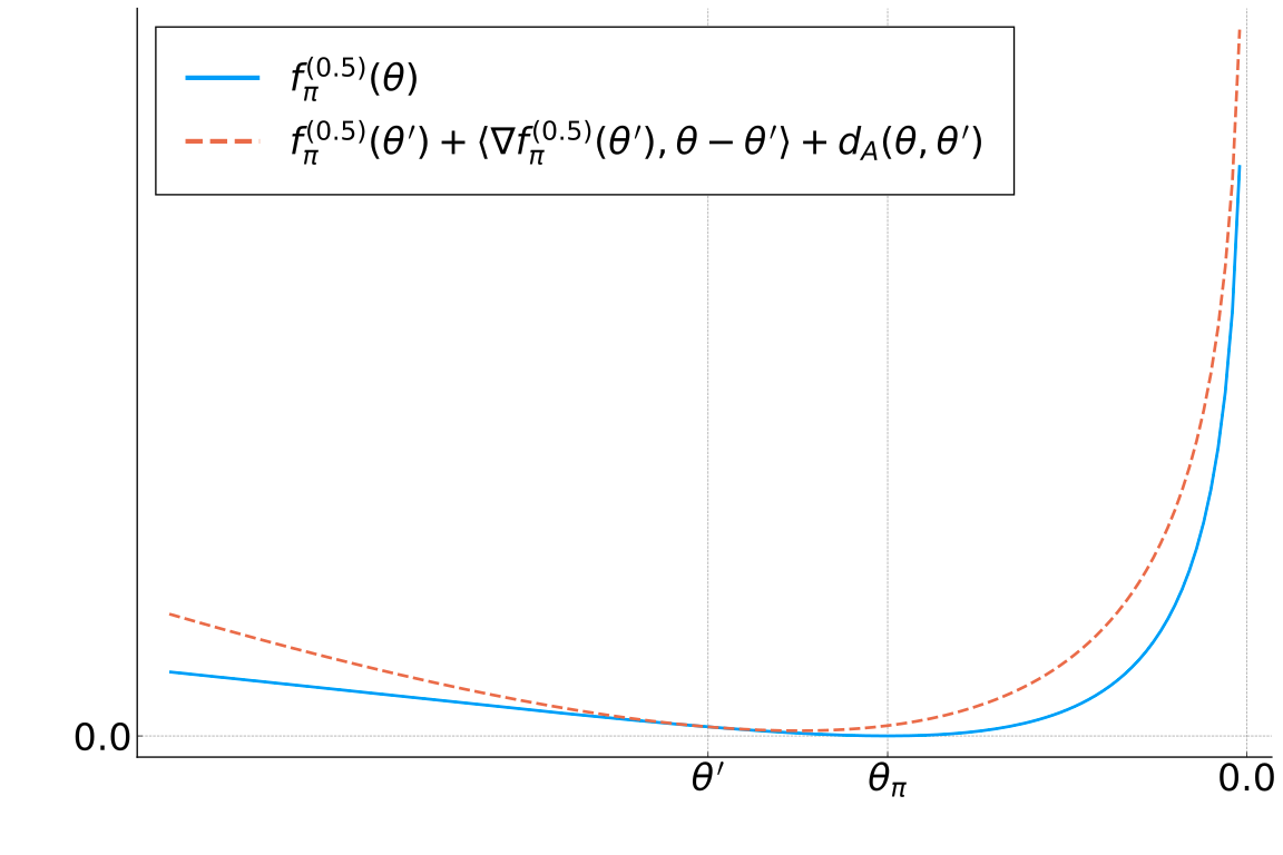
(a) Relative smoothness illustrated in the case $\alpha=0.5$

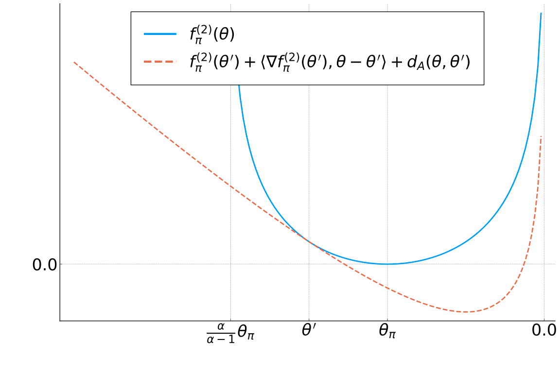
(b) Relative strong convexity shown in the case $\alpha=2$

Figure 1: Plots of $f_{\pi}^{(\alpha)}$ and the tangent approximations described in Definition 9, obtained by choosing $\mathcal{Q}=\mathcal{G}_{0}^{1}$ and $\pi\in\mathcal{G}_{0}^{1}$ equal to some $q_{\theta_{\pi}}$.

Figure 1 illustrates the results of Proposition 9 when the exponential family is the family of centered one-dimensional Gaussians $\mathcal{G}_{0}^{1}$ and the target as well belongs to this family. One can see that, when $\alpha\leq 1$, relative smoothness is satisfied and $f_{\pi}^{(\alpha)}$ is above its tangent approximation. On the contrary, $\alpha\geq 1$ yields relative strong convexity, ensuring that $f_{\pi}^{(\alpha)}$ is above its tangent approximation.

We now give a result about potential failures of the Euclidean smoothness of $f_{\pi}^{(\alpha)}$. This suggests that the Euclidean metric is not well-suited to minimize $f_{\pi}^{(\alpha)}$.

Proposition 11.

There exist targets $\pi$ and exponential families $\mathcal{Q}$ such that the gradient of $f_{\pi}^{(\alpha)}$ is not Lipschitz on $\operatorname*{dom}f_{\pi}^{(\alpha)}$, for $\alpha>0$.

Proof.

See Appendix A.7 ∎

Remark 5.

The complete proof is in Appendix A. Let us exhibit counter-examples built by using $\mathcal{Q}=\mathcal{G}^{1}_{0}$ and targets $q_{\theta_{\pi}}\in\mathcal{G}^{1}_{0}$. Recall that $(f_{\pi}^{(\alpha)})^{\prime}$ is Lipschitz continuous on its domain if and only if $(f_{\pi}^{(\alpha)})^{\prime\prime}$ is bounded on its domain. In our setting, we have

$$\operatorname*{dom}f_{\pi}^{(\alpha)}=\begin{cases}\Theta&\text{ if }\alpha\leq 1,\\ (\frac{\alpha}{\alpha-1}\theta_{\pi},0)&\text{ if }\alpha>1,\end{cases}$$

and $|(f_{\pi}^{(\alpha)})^{\prime\prime}(\theta)|\rightarrow+\infty$ when $\theta\rightarrow 0$, and also when $\theta\rightarrow\frac{\alpha}{\alpha-1}\theta_{\pi}$ for the case $\alpha>1$.

The counter-example used in the proof of Proposition 11 illustrates why choosing to work in the Bregman geometry induced by $A$ can be beneficial. Indeed, when $\alpha\in(0,1]$, we have relative smoothness from Proposition 9, while Euclidean smoothness fails. In this case, Euclidean smoothness might be recovered if we restricted $f_{\pi}^{(\alpha)}$ to some set of the form $[\epsilon,+\infty)$. However, this would create a risk of excluding the target value $\theta_{\pi}$ by choosing $\epsilon$ too large.

This counter-example is also a case where Assumption 1 (i) fails for $\alpha>1$ since $\operatorname*{dom}f_{\pi}^{(\alpha)}$ is strictly included in $\Theta$. One could also restrict the search to a smaller set, but the upper bound of $\operatorname*{dom}f_{\pi}^{(\alpha)}$ would depend on the target true parameters. This prevents from restricting the admissible values of $\theta$ in a meaningful way without tight knowledge on the target. Note also that the family $\mathcal{G}_{0}^{1}$ has a log-partition function $A$ that is not strongly convex. Finally the family $\mathcal{G}_{0}^{1}$ also allows us to show that, even for a log-concave target $\pi\in\mathcal{G}_{0}^{1}$, the objective function $f_{\pi}^{(\alpha)}$ might not be convex, as illustrated in Figure 2.

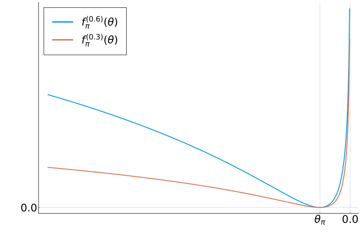
Figure 2: Plots of $f_{\pi}^{(\alpha)}$ for two values of $\alpha\in(0,1)$, obtained following the setting described in the proof of Proposition 11.

Figure 2 shows a situation where the function $f_{\pi}^{(\alpha)}$ is not convex, but has a unique stationary point, which is the global minimizer. We show now that this situation is implied by having $\pi=q_{\theta_{\pi}}$ for some $\theta_{\pi}\in\operatorname*{int}\Theta$. In this case, it is also possible to derive further results.

Proposition 12.

Suppose that Assumption 1 and verified and that there exists $\theta_{\pi}\in\operatorname*{int}\Theta$ with $\pi=q_{\theta_{\pi}}$. Then Assumption 2 is verified, and the function $f_{\pi}^{(\alpha)}$ has a unique minimizer, which is $\theta_{\pi}$ and which is also its only stationary point. Moreover, $\vartheta_{\pi}^{(\alpha)}=f_{\pi}^{(\alpha)}(\theta_{\pi})=0$.

Proof.

See Appendix A.8 ∎

Proposition 12 shows that when $r\equiv 0$ and $\pi=q_{\theta_{\pi}}$ with $\theta_{\pi}\in\operatorname*{int}\Theta$, the stationary point of Problem ($P_{\pi}^{(\alpha)}$) is unique and equal to the global minimizer of this problem. The next proposition investigate the behavior of $f_{\pi}^{(\alpha)}$ around its minimizer $\theta_{\pi}$.

Proposition 13.

Consider $\theta\in\operatorname*{int}\Theta$ in a neighborhood of $\theta_{\pi}$ of the form $B(\theta_{\pi},\upsilon)$ for some $\upsilon>0$. Then, for any $\alpha>0,\alpha\neq 1$, we have that

1. $f_{\pi}^{(\alpha)}$ has a quadratic behavior in the neighborhood of $\theta_{\pi}$, i.e. $f_{\pi}^{(\alpha)}(\theta)=\frac{\alpha}{2}\|\theta-\theta_{\pi}\|^{2}_{\nabla^{2}A(\theta_{\pi})}+o(\upsilon^{2})$,

2. $f_{\pi}^{(\alpha)}$ satisfies a Polyak-Łojasiewicz inequality around $\theta_{\pi}$: $f_{\pi}^{(\alpha)}(\theta)\leq\frac{1}{2\alpha}\|\nabla f_{\pi}^{(\alpha)}(\theta)\|^{2}_{\nabla^{2}A^{*}(\nabla A(\theta_{\pi}))}+o(\upsilon^{2})$.

Proof.

See Appendix A.9 ∎

Proposition 13 shows that, in the neighborhood of its minimizer, function $f_{\pi}^{(\alpha)}$ has a quadratic behavior, hence generalizing a known result in the case $\alpha=1$ [2]. It also shows that $f_{\pi}^{(\alpha)}$ satisfies a type of Polyak-Łojasiewicz inequality around the point $\theta_{\pi}$. This type of condition has been used to prove geometric rates of convergence to minimizers for a variety of optimization algorithm, while being weaker than strong convexity [57].

5.2 Convergence analysis of Algorithm 1 and Algorithm 2

We are now ready to present our convergence results for Algorithm 1. We give a first set of results for values of $\alpha$ in $(0,1]$, and then stronger results when $\alpha=1$. Results for $\alpha\in(0,1]$ only exploit the relative smoothness, while the results for $\alpha=1$ rely on the relative smoothness and the relative strong convexity of $f_{\pi}^{(1)}$.

We now give our convergence results for Algorithm 1 for $\alpha\in(0,1]$.

Proposition 14.

Consider a sequence $\{\theta_{k}\}_{k\in\mathbb{N}}$ generated by Algorithm 1 from $\theta_{0}\in\operatorname*{int}\Theta$, with $\alpha\in(0,1]$ and a sequence of step-sizes $\{\tau_{k}\}_{k\in\mathbb{N}}$ such that $\tau_{k}\in(0,1]$. Under Assumptions 1, 2, and 3,

1. the sequence $\{F_{\pi}^{(\alpha)}(\theta_{k})\}_{k\in\mathbb{N}}$ is non-increasing,

2. if $F_{\pi}^{(\alpha)}(\theta_{K+1})=F_{\pi}^{(\alpha)}(\theta_{K})$ for some $K\in\mathbb{N}$, then $\theta_{k}=\theta_{K}$ for every $k\geq K$ and $\theta_{K}$ is a stationary point of $F_{\pi}^{(\alpha)}$,

3. $\sum_{k\geq 0}KL(q_{\theta_{k}},q_{\theta_{k+1}})<+\infty$,

4. let $K\in\mathbb{N}$ the first iterate such that $d_{A}(\theta_{K},\theta_{K+1})\leq\varepsilon$ for some $\varepsilon>0$. Then $K$ is at most equal to $\frac{1}{\varepsilon}\left(F_{\pi}^{(\alpha)}(\theta_{0})-\vartheta_{\pi}^{(\alpha)}\right)$.

5. if in addition, there exists a non-empty compact set $C\subset\operatorname*{int}\Theta$ such that $\theta_{k}\in C$ for every $k\in\mathbb{N}$ and $r$ is continuous on $C$, and a scalar $\epsilon>0$ such that $\tau_{k}\in[\epsilon,1]$ for every $k\in\mathbb{N}$, then every converging subsequence of $\{\theta_{k}\}_{k\in\mathbb{N}}$ converges to a point in $S_{\pi}^{(\alpha)}$.

Proof.

See Appendix B.1 ∎

The additional assumption used for Prop. 14(v) is satisfied for instance if $r=\iota_{C}$, for a compact $C\subset\operatorname*{int}\Theta$. The continuity assumption on $r$ is also satisfied by the $\ell_{1}$ norm. In this case, $r$ is also coercive, ensuring that the iterates stay in a compact set. However, this does not ensure that the iterates do not approach the boundary of $\Theta$. Note that when $S_{\pi}^{(\alpha)}=\{\theta_{s}\}$ for some $\theta_{s}\in\operatorname*{int}\Theta$, Prop. 14(v) implies that $\theta_{k}\xrightarrow[k\rightarrow+\infty]{}\theta_{s}$.

We now refine the result of Proposition 14 in the case $\alpha=1$. In this case, the function $f_{\pi}^{(\alpha)}$ is also relatively strongly convex and coercive, two properties that are used to give stronger results, including rates of convergence to the global minimizer.

Proposition 15.

Consider a sequence $\{\theta_{k}\}_{k\in\mathbb{N}}$ generated by Algorithm 1 from $\theta_{0}\in\operatorname*{int}\Theta$, with $\alpha=1$ and a sequence of step-sizes $\{\tau_{k}\}_{k\in\mathbb{N}}$ such that $\tau_{k}\in[\epsilon,1]$ for some $\epsilon>0$. Consider the point $\theta_{*}$ defined in Proposition 10. Under Assumptions 1, 2, and 3,

1. the sequence $\{KL(q_{\theta_{k}},q_{\theta_{*}})\}_{k\in\mathbb{N}}$ is non-increasing and

   $$KL(q_{\theta_{k}},q_{\theta_{*}})\leq(1-\epsilon)^{k}KL(q_{\theta_{0}},q_{\theta_{*}}),\quad\forall k\in\mathbb{N},$$

2. we have that $F_{\pi}^{(1)}(\theta_{k})\xrightarrow[k\rightarrow+\infty]{}F_{\pi}^{(1)}(\theta_{*})=\vartheta_{\pi}^{(1)}$ and that

   $$F_{\pi}^{(1)}(\theta_{k})-F_{\pi}^{(1)}(\theta_{*})\leq\frac{(1-\epsilon)^{k}}{\epsilon}KL(q_{\theta_{0}},q_{\theta_{*}}),\quad\forall k\in\mathbb{N},$$

3. the iterates converge to the solution, $\theta_{k}\xrightarrow[k\rightarrow+\infty]{}\theta_{*}$.

Proof.

See Appendix B.2 ∎

Remark 6.

We can see in the above that if $\epsilon=1$, then $KL(q_{\theta_{1}},q_{\theta_{*}})=0$, meaning that $\theta_{1}=\theta_{*}$ and that the optimal value is reached in one iteration. This is because of the particular structure of the Bregman gradient operator when $\alpha,\tau=1$. Indeed, under Assumption 2, there exists $\theta^{(1)}\in\operatorname*{int}\Theta$ such that $\pi(\Gamma)=q_{\theta^{(1)}}(\Gamma)$, so for every $\theta\in\operatorname*{int}\Theta$, $\gamma_{f_{\pi}^{(1)}}^{A}(\theta)=\theta^{(1)}$ (using Eq. (6) and Proposition 8) and $\theta_{1}=\text{prox}_{r}^{A}(\theta^{(1)})$. So $\text{prox}_{r}^{A}(\theta^{(1)})=\theta_{*}$. Note that this phenomenon does not happen for Algorithm 2, where $\pi(\Gamma)$ is approximated, or when the proximal step is not computed exactly.

We now present a specialized result for the case $\alpha\in(0,1)$, $r\equiv 0$, under the assumption that $\pi=q_{\theta_{\pi}}$ for some $\theta_{\pi}\in\operatorname*{int}\Theta$. In this case, we are able to derive convergence results that are similar to the case $\alpha=1$.

Proposition 16.

Consider a sequence $\{\theta_{k}\}_{k\in\mathbb{N}}$ generated by Algorithm 1 from $\theta_{0}\in\operatorname*{int}\Theta$, with $\alpha\in(0,1)$ and a sequence of step-sizes $\{\tau_{k}\}_{k\in\mathbb{N}}$ such that $\tau_{k}\in[\epsilon,1]$ for some $\epsilon>0$. Assume that the iterates stay in a non-empty compact set $C\subset\operatorname*{int}\Theta$, that $r\equiv 0$, that there exists $\theta_{\pi}\in\operatorname*{int}\Theta$ such that $\pi=q_{\theta_{\pi}}$, and that Assumption 1 is satisfied. Then,

1. $RD_{\alpha}(\pi,q_{\theta_{k}})\xrightarrow[k\rightarrow+\infty]{}0$ and there exist constants $C>0$ and $\delta\in(0,1)$ such that

   $$RD_{\alpha}(\pi,q_{\theta_{k}})\leq C(1-\alpha\delta\epsilon)^{k}RD_{\alpha}(\pi,q_{\theta_{0}}),\quad\forall k\in\mathbb{N},$$

2. $\theta_{k}\xrightarrow[k\rightarrow+\infty]{}\theta_{\pi}$.

Proof.

See Appendix B.3 ∎

Remark 7.

Due to the skew-symetry of $RD_{\alpha}$ for $\alpha\in(0,1)$ [95, Proposition 2], we have, under the same hypotheses, that $RD_{1-\alpha}(q_{\theta_{k}},\pi)\xrightarrow[k\rightarrow+\infty]{}0$ with the same rate of convergence. Note also that Proposition 16 can be extended, in a straightforward manner, to the case when $r=\iota_{C}$ with $C$ such that $\theta_{\pi}\in\operatorname*{int}C$ and Assumption 3 is satisfied.

We now address the link between Algorithms 1 and 2. In particular, we show that the former is the limit of the latter when the number of samples goes to infinity.

Proposition 17.

Assume that Assumptions 1, 2, and 3 are satisfied. Consider a sequence $\{(\hat{\theta}_{k},\hat{\theta}_{k+\frac{1}{2}})\}_{k\in\mathbb{N}}$ generated by Algorithm 2 and a sequence $\{(\theta_{k},\theta_{k+\frac{1}{2}})\}_{k\in\mathbb{N}}$ generated by Algorithm 1 such that the two algorithms use the same settings and $\theta_{0}=\hat{\theta}_{0}$.

Assume either that $r\equiv 0$ and that Algorithm 2 generates iterates $\{\hat{\theta}_{k}\}_{k\in\mathbb{N}}$ that belong to $\operatorname*{int}\Theta$ with probability one, or that there exists a non-empty compact set $C\subset\operatorname*{int}\Theta$ such that the iterates $\{\theta_{k}\}_{k\in\mathbb{N}},\{\hat{\theta}_{k}\}_{k\in\mathbb{N}}$ belong to $C$ and the iterate $\{\theta_{k+\frac{1}{2}}\}_{k\in\mathbb{N}},\{\hat{\theta}_{k+\frac{1}{2}}\}_{k\in\mathbb{N}}$ belong to $\operatorname*{int}\Theta$ with probability one. If $N_{k}\rightarrow+\infty$ for every $k\in\llbracket 1,K\rrbracket$, then

$$\hat{\theta}_{k}\rightarrow\theta_{k}\text{ almost surely}$$

for every $k\in\llbracket 1,K\rrbracket$.

Proof.

See Appendix B.4 ∎

Note that this result is independent of the behavior of $\{\theta_{k}\}_{k\in\mathbb{N}}$. In the case $r\not\equiv 0$, the additional assumption on the iterates is satisfied for instance if $r=\iota_{C}$, for a compact $C\subset\operatorname*{int}\Theta$.

5.3 Discussion

Proposition 14 implies a monotonic decrease of $F_{\pi}^{(\alpha)}$ along iterations of Algorithm 1. This kind of result appears in many statistical procedures [37, 24, 33, 34]. Note that these works encompass more general approximating families than our study, but do not consider our additional regularization term $r$. In our setting, we are moreover able to give novel and more precise results on the convergence of the sequence of iterates. The result of Proposition 14 (iii), which is a type of finite length property of the sequence of iterates, is not common for a statistical procedure, to our knowledge. This result can be used to practically assess the convergence of our algorithms as the condition $KL(q_{\theta_{k}},q_{\theta_{k+1}})\leq\varepsilon$ can be employed as a stopping criterion in Algorithms 1 and 2. Proposition 14 (iv) provides estimates on the number of iterations needed to reach a certain level of stationarity between iterates, while Proposition 14 (v) establishes convergence to the set of stationary points.

We are also able to show the linear geometric rate of convergence to the global minimizer of Problem ($P_{\pi}^{(\alpha)}$) when $\alpha=1$ in Proposition 15 and when $\pi\in\mathcal{Q}$ and $r\equiv 0$ for $\alpha<1$ in Proposition 16. Note that the result for $\alpha=1$ is established under minimal assumptions on $\pi$ as we only need $\pi(\Gamma)$ to be well-defined (see Assumption 2). In comparison, similar rates of convergence are established in the case of the objective function $KL(\cdot,\pi)$ in [65, 99] under strong log-concavity and log-smoothness assumptions on $\pi$. We are not aware of any VI algorithm achieving geometric rates such as ours in the case of the Rényi divergence. Let us however mention that, in the context of sampling algorithms, a geometric convergence of the probability distribution of the samples to the minimizer of $RD_{\alpha}(\cdot,\pi)$ for $\alpha\geq 1$ is proven in [97] under log-smoothness assumption on the target and a weaker version of log-concavity. It is difficult to compare the assumption $\pi\in\mathcal{Q}$ with log-concavity or log-smoothness assumptions, as some exponential families might have multi-modal members or can be written over a discrete space $\mathcal{X}$.

More generally, we avoided in our analysis any assumption that would not be satisfied by the one-dimensional Gaussian target described in Example 4. Therefore, we are facing a situation where $\nabla f_{\pi}^{(\alpha)}$ is not Lipschitz, $A$ is not strongly convex, and $\operatorname*{dom}A$ is not closed, which contrasts with common assumptions from the literature on optimization schemes based on Bregman divergences [13, 93, 18, 44, 47] or in the statistical literature [1, 59, 66]. Note that the Euclidean smoothness of $KL(\cdot,\pi)$ is proven for instance in [36, 65] under log-smoothness assumption on the target. However, when Euclidean smoothness is not satisfied and a standard gradient descent method is used, tuning the step-size, or learning rate, cannot be done using the Lipschitz constant of the gradients. In Section 6, we compare the VRB method of [66], which can be seen as an Euclidean counterpart to our Algorithm 2 (see Section 4.2.2). We show that the lack of information about the Lipschitz constant creates instabilities and poor performance, in contrast to our proposed method where the step-sizes can be chosen following the results presented in Propositions 14 and 15.

Finally, Proposition 17 connects Algorithm 1, which is deterministic, and Algorithm 2, based on stochastic sampling, by showing that the former is a limit version of the latter when the number of samples grows to infinity. This result is similar to [37, Proposition 5.1] although the considered approximating families are not the same and we here consider $\alpha\neq 1,r\not\equiv 0$. As in the moment-matching scheme of [70, Theorem 3.2], we require all the sample sizes to converge to infinity, but our result allows to consider a broader situation with $\alpha\neq 1$ and the use of a proximal step. Unlike ours, the convergence results of the stochastic schemes in [65, 99] do not require sample size going to infinity, which might be explained since our estimators of $\pi_{\theta}^{(\alpha)}(\Gamma)$ are only asymptotically unbiased, which is not the case in the schemes of [99, 65], based on Wasserstein gradients flows.

Our convergence analysis is restricted to $\alpha\in(0,1]$, which is also the case in [34], considering the minimization of the $\alpha$-divergence $D_{\alpha}$ over wider families. The convergence proof techniques used in this work actually share some common points with ours. In particular, because of the $1$-relative smoothness of $f_{\pi}^{(\alpha)}$ with respect to $A$, we have from Definition 9 that

$$f_{\pi}^{(\alpha)}(\theta)-f_{\pi}^{(\alpha)}(\theta^{\prime})\leq\langle q_{\theta^{\prime}}(\Gamma)-\pi_{\theta^{\prime}}^{(\alpha)}(\Gamma),\theta-\theta^{\prime}\rangle+KL(q_{\theta^{\prime}},q_{\theta}).$$ (22)

This is to be compared with [34, Proposition 1], which, in our setting, woud read

$$\Psi_{\pi}^{(\alpha)}(\theta)-\Psi_{\pi}^{(\alpha)}(\theta^{\prime})\leq-\frac{1}{\alpha}\int\pi(x)^{\alpha}q_{\theta^{\prime}}(x)^{1-\alpha}\log\left(\frac{q_{\theta}(x)}{q_{\theta^{\prime}}(x)}\right)\nu(dx).$$ (23)

Note that here, $q_{\theta},q_{\theta^{\prime}}$ are not necessarily from an exponential family and that we used $\Psi_{\pi}^{(\alpha)}(\theta)=D_{\alpha}(\pi,q_{\theta})$, while $D_{\alpha}(q_{\theta},\pi)$ was considered in [34] (this does not affect the results as $D_{\alpha}(\pi,q_{\theta})=D_{1-\alpha}(q_{\theta},\pi)$ for $\alpha\in[0,1]$). When $q_{\theta}$ and $q_{\theta^{\prime}}$ are in an exponential family $\mathcal{Q}$, Eq. (23) can be further rewritten as

$$\Psi_{\pi}^{(\alpha)}(\theta)-\Psi_{\pi}^{(\alpha)}(\theta^{\prime})\leq\frac{Z_{\pi_{\theta^{\prime}}^{(\alpha)}}}{\alpha}\left(\langle q_{\theta^{\prime}}(\Gamma)-\pi_{\theta^{\prime}}^{(\alpha)}(\Gamma),\theta-\theta^{\prime}\rangle+KL(q_{\theta^{\prime}},q_{\theta})\right),$$ (24)

with $Z_{\pi_{\theta^{\prime}}^{(\alpha)}}=\int\pi(x)^{\alpha}q_{\theta^{\prime}}(x)^{1-\alpha}\nu(dx)$. We recognize now that the right-hand side of Eq. (24) is equal to the one of (22) up to a positive multiplicative constant. Even if the result of [34, Proposition 1] is derived directly without using Bregman divergences, our analysis gives a geometric interpretation to it. Moreover, our interpretation allows to use the modern Bregman proximal gradient machinery, allowing to prove convergence results that are more precise while including the additional regularization term $r$. Indeed, the convergence result in [34] only shows a monotonic decrease of the objective without regularization, although in wider variational families.

In another context, it is often not straightforward to choose the most adapted statistical divergence for a given application. Indeed, there are many types of statistical divergences that are indexed by a scalar parameter, for some value of which the KL divergence is recovered [27]. There exist some comparative studies [45], but they are restricted to particular contexts. The notions of relative smoothness and relative strong convexity allow us to show that the KL divergence can be used to construct tangent majorizations or minorization of the Rényi divergences, which seems to be a new insight and may help guide the choice of a divergence.

6 Numerical experiments

In this section, we investigate the performance of our methods through numerical simulations in a black-box setting and compare them with existing algorithms. We focus our study on Algorithm 2, that we call the relaxed moment-matching (RMM) algorithm when $r\equiv 0$ and the proximal relaxed moment-matching (PRMM) otherwise. We also consider VRB algorithm from [66], whose implementation for an exponential family is described in Algorithm 3. It is shown in Section 4.2.2 that the VRB algorithm can be interpreted as an Euclidean version of our novel RMM algorithm. However, when $\alpha\in(0,1]$, $f_{\pi}^{(\alpha)}$ is not smooth relatively to the Euclidean distance (see Proposition 11) while it is smooth relatively to the Bregman divergence $d_{A}$ (see Proposition 9). Therefore, the comparison between the RMM and PRMM algorithms with the VRB method might allow to assess the use of the Bregman divergence instead of the Euclidean distance on a numerical basis. We also use this comparison to assess the role of the regularizer, which is a feature of our approach, but not of [66].

Additional numerical experiments are presented in Appendix D. In particular, the influence of the parameters $\alpha$ and $\tau$ and of the regularizer $r$ is studied in Appendix D.1 using a Gaussian toy example. In Appendix D.2, we provide additional comparison between the RMM and the VRB algorithms. We now turn to a Bayesian regression task, which allows us to compare the RMM, PRMM and VRB algorithms on a realistic problem and understand better the interest of using the Bregman geometry. We also use this example to show how our PRMM algorithm allows to compensate for a misspecified prior by adding a regularizer.

We consider a problem of non-linear regression, where we try to infer a regression vector $\beta\in\mathbb{R}^{d+1}$ from $J$ measurements $y\in\mathbb{R}^{J}$, $X\in\mathbb{R}^{J\times d}$ under Gaussian noise. The non-linearity mimics the effect of a neural network with one single hidden layer,

$$\Phi_{\beta}(x)=\phi\left(\sum_{i=1}^{d}\beta_{i}x_{i}+\beta_{0}\right),\,\forall x\in\mathbb{R}^{d},$$

where $\beta=(\beta_{i})_{0\leq i\leq d+1}\in\mathbb{R}^{d+1}$ is the regression vector, with the component $\beta_{0}$ playing the role of the bias. The function $\phi$ is the activation function and is taken here as the sigmoid function

$$\phi(s)=\frac{1}{1+e^{-s}},\,\forall s\in\mathbb{R}.$$

Given a ground truth vector $\overline{\beta}\in\mathbb{R}^{d+1}$, and a feature set $X$, we assume, for every $j\in\{1,\ldots,J\}$,

$$y_{j}\sim\mathcal{N}\left(y_{j};\Phi_{\overline{\beta}}(X_{j}),\sigma^{2}\right),$$

with $X_{j,:}$ the $j$-th line of $X$, and $X_{j}=X_{j,:}^{\top}\in\mathbb{R}^{d}$. Assuming i.i.d. realizations, this leads to the likelihood expression for a given $\beta\in\mathbb{R}^{d+1}$,

$$p(y|\beta)=\prod_{j=1}^{J}\mathcal{N}\left(y_{j};\Phi_{\beta}(X_{j}),\sigma^{2}\right).$$

Our goal is to explore the posterior distribution on $\beta$,

$$p(\beta|y)=\frac{p(y|\beta)p(\beta)}{p(y)},$$

where knowledge on the regression vector $\beta$ is encoded in a prior density $p(\beta)$. In the following, we drop the dependence on the data, so that our target reads

$$\pi(\beta):=p(\beta|y)\text{ and }\tilde{\pi}(\beta):=p(\beta|y)p(\beta).$$

The RMM, PRMM, and VRB algorithm are tested on synthetic data. First, a regression vector $\overline{\beta}$ is sampled from a spike-and-slab distribution

$$p_{0}(\beta)=\mathcal{N}(\beta_{0};0.0,1.0)\prod_{i=1}^{d}\left(\rho\delta_{0}(\beta_{i})+(1-\rho)\mathcal{N}(\beta_{i};0.0,1.0)\right).$$

which places a non-zero probability on $\beta_{i}$ being zero, for $i\in\llbracket 1,d\rrbracket$. This type of distribution is called a Gaussian-zero model in [83] and is linked with Bernoulli-Gaussian models. Regression vectors are sampled until we find $\bar{\beta}\sim p_{0}$ with at least one zero and one non-zero component.

Then, for every $j\in\llbracket 1,J\rrbracket$, we sample vectors $X_{j}$ uniformly in the square $[-s,s]^{d}$ and draw the observation $y_{j}$ as stated before. Test data $y^{\text{test}}\in\mathbb{R}^{J_{test}}$ and $X\in\mathbb{R}^{J_{test}\times d}$ are also generated in this manner. We consider a Gaussian prior on $\beta$, $p(\beta)=\mathcal{N}(\beta;0,I)$.

Since $\overline{\beta}$ is not sampled from the prior $p(\beta)$, there is a mismatch between the data we feed the algorithms and the posterior model. In the following, we show that the choice of a suitable regularizer in our VI method can allow to cope with this issue.

We run experiments using the VRB and RMM algorithms, as well as the PRMM algorithm, using the family of Gaussian densities with diagonal covariance matrix, whose parametrization is detailed in Appendix C. For the PRMM algorith, we use the regularizer

$$r(\theta)=\eta\|\theta_{1}\|_{1},$$

with $\eta\geq 0$. This can be understood as the Lagrangian relaxation [51] with multiplier $\eta\geq 0$ of the constraint

$$\sum_{i=1}^{d}\|\theta_{1}\|_{1}\leq c,$$

for $c\geq 0$ such that the constrained set is non empty.

Our $\ell_{1}$-like regularizer enforces sparsity on all the components of the mean $\mu$, except the component $\mu_{0}$. The aim is to mimic the sparse structure of $\overline{\beta}$ that was simulated from $p_{0}$. The computation of the corresponding Bregman proximal operator for this choice of $r$ is detailed in Appendix C.

The algorithms are run for $K=100$ iterations, with a constant number of samples $N=500$. Two values of $\alpha$ are tested, namely, $\alpha=1.0$ and $\alpha=0.5$. The VRB algorithm is run with $\tau=10^{-3}$ while the PRMM algorithm is run with $\tau=10^{-1}$. These choices correspond to the most favorable step-size for each algorithm, as indicated by our experiments in Appendix D. The algorithms are run $10^{3}$ times. We choose $\eta=1.0$ in the following. In the subsequent experiments, we set $d=5$, $J=100$, $J^{\text{test}}=50$, $\sigma^{2}=0.5$, and $s=5.0$.

In order to asses the performance of the algorithm, we track the variational Rényi bound, defined Eq. (20), that is estimated at each iteration $k\in\mathbb{N}$ through

$$\mathcal{L}_{\pi}^{(\alpha)}(\theta_{k})\approx\frac{1}{\alpha}\log\left(\frac{1}{N_{k+1}}\sum_{l=1}^{N_{k+1}}w_{l}^{(\alpha)}\right).$$ (25)

We also consider the F1 score that each algorithm achieves in the prediction of the zeros of the true regression vector $\overline{\beta}$. It is computed at each iteration $k\in\mathbb{N}$, by seeing how the zeros of $\mu_{k}$ match those of $\overline{\beta}$.

Additionally, since we provide not only a pointwise estimate of $\overline{\beta}$, but an approximation of the full target $\pi$, we also test the quality of the distributional approximation by sampling a regression vector $\beta$ from the final proposal $q_{\theta_{K}}$. This is done by computing

$$\text{MSE}^{\text{test}}(\beta):=\sum_{j=1}^{J^{\text{test}}}\left(y_{j}^{\text{test}}-\Phi_{\beta}(X_{j}^{\text{test}})\right)^{2}.$$

By sampling $N^{\text{test}}_{\beta}$ vectors $\beta\sim q_{\theta_{K}}$ and analyzing the distribution of the values $\{\text{MSE}^{\text{test}}(\beta_{l})\}_{l=1}^{N^{\text{test}}_{\beta}}$, we can get a sense of the quality of the approximated density $q_{\theta_{K}}$ in terms of both location and scale. At each run, the final distribution $q_{\theta_{K}}$ is tested by sampling $N^{\text{test}}_{\beta}=100$ values of $\beta$ to assess the test error.

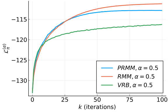
(a) $\alpha=0.5$

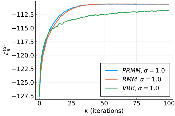
(b) $\alpha=1.0$

Figure 3: Approximated Rényi bound, averaged over $10^{3}$ runs with $N=500$ samples per iteration.

Figure 3 shows the increase of the approximated variational Rényi bound described in Eq. (25). As discussed in Section 4.2.2, an increase in the Rényi bound $\mathcal{L}_{\pi}^{(\alpha)}(\theta)$ shows a decrease in the Rényi divergence $RD_{\alpha}(\pi,q_{\theta})$, so these plots show that the three method decrease the Rényi divergence. However, our methods are able to reach higher values at a faster rate than the VRB method, illustrating the improvement coming from using the Bregman geometry rather than the Euclidean one.

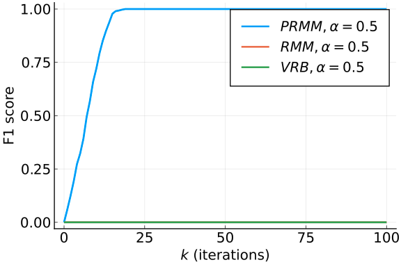
(a) $\alpha=0.5$

(b) $\alpha=1.0$

Figure 4: F1 score in the prediction of the zeros of $\overline{\beta}$ by the zeros of $\{\mu_{k}\}_{k=0}^{K}$, averaged over $10^{3}$ runs with $500$ samples per iteration.

Figure 4 shows the F1 score achieved by each algorithm in the retrieval of the zeros of the true regression vector. The RMM and VRB algorithms are not able to recover any zeros, which is to be expected since they do not include any sparsity-inducing mechanisms. However, the PRMM algorithm is able to recover in this example the zero components of the regression vector in a few number of iterations and in most of the runs. Note also that it does not create false positives neither. This illustrates that adding a regularizer in the VI method itself can enforce sparsity although the prior of our model did not enforce it.

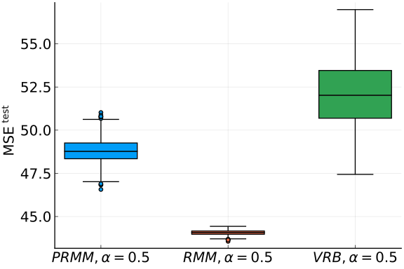
(a) $\alpha=0.5$

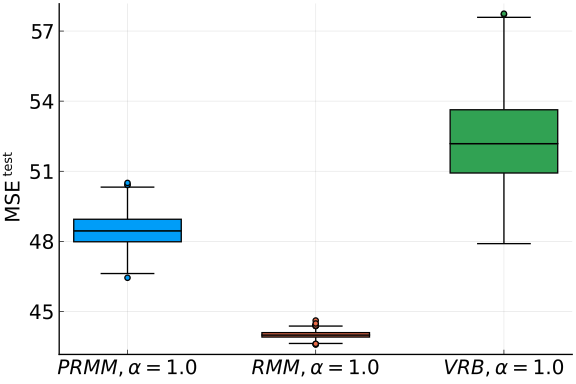
(b) $\alpha=1.0$

Figure 5: Box plots of the values $\text{MSE}^{\text{test}}$, showing the reconstruction errors on the test data.

The box plots of Fig. 5 assess the quality of the variational approximation of the posterior obtained by each method, by evaluating how regression vectors sampled from the approximations are able to reconstruct the test data. We see that the PRMM and RMM algorithms yields reconstruction errors that are less spread and at a lower level than the ones coming from the VRB algorithm. This is in accordance with the plots of Fig. 3. This shows the higher performance coming from using a more adapted geometry. Note that errors are more spread for the PRMM algorithm than for the RMM algorithm. This may be due to the proximal step, which creates bigger eigenvalues for the covariance matrix (see Appendix C for details).

In this section, we observed that the RMM and PRMM are able to obtain better performance than the VRB algorithm in terms of Rényi bound and reconstruction errors, while recovering all the correct zeros of the regression vector using a regularizer. This shows the interest of using the geometry induced by the KL divergence and additional regularizer terms.

7 Conclusion and perspectives

We introduced in this work the proximal relaxed moment-matching algorithm, which is a novel VI algorithm minimizing the sum of a Rényi divergence and a regularizing function over an exponential family. We provided a black-box implementation which allows to bridge the gap between information-geometric VI methods and black-box VI algorithms, while generalizing several existing moment-matching algorithms. We also rewrote our algorithm as a Bregman proximal gradient algorithm whose Bregman divergence is equivalent to the Kullback-Leibler divergence.

Using this novel perspective, we established strong convergence guarantees for our exact algorithm. For $\alpha\in(0,1]$, we established the monotonic decrease of the objective function, a finite-length property of the sequence of iterates, and subsequential convergence to a stationary point. In the particular case $\alpha=1$, we also established the geometric convergence of the iterates towards the optimal parameters. We also exhibited a simple counter-example for which the corresponding Euclidean schemes may fail to converge, showing the necessity of resorting to an adapted geometry. These findings are backed by numerical results showing the versatility of our methods compared to more restricted moment-matching updates. Indeed, our parameters allow to tune the algorithms speed and robustness but also the features of the approximating densities. Comparison of our algorithms with their Euclidean counterparts also showed their robustness and good performance.

This confirmed the benefits of using a regularized Rényi divergence and the underlying geometry of exponential families, but also opened several research avenues.

First, although we proved the convergence of Algorithm 1, work remains to be done to establish the convergence of Algorithm 2. In particular, it would be interesting to understand the interplay between $\alpha$, the step-sizes $\{\tau_{k}\}_{k\in\mathbb{N}}$ and the sample sizes $\{N_{k}\}_{k\in\mathbb{N}}$. Approximation errors can arise for a too low sample size, or when the proximal step is computed with limited precision. Analyzing the algorithm stability with error propagation quantification in such cases is another interesting challenge. Then, another venue of improvement would be the use of more complex optimization schemes, such as block updates or accelerated schemes. Variance reduction techniques as used in some black-box VI algorithms could also be used to improve our Algorithms. Finally, studying optimization schemes over mixtures of distributions from an exponential family could be a natural extension in order to tackle multimodal targets. Similarly, extending our analysis to values $\alpha>1$ would allow to use the $\chi^{2}$ divergence, which plays an important role for the analysis of importance sampling schemes.

Funding

T.G. and E.C. acknowledge support from the ERC Starting Grant MAJORIS ERC-2019-STG-850925. The work of V. E. is supported by the Agence Nationale de la Recherche of France under PISCES (ANR-17-CE40-0031-01), the Leverhulme Research Fellowship (RF-2021-593), and by ARL/ARO under grant W911NF-22-1-0235.

Supplementary material (Appendices A-D)

Appendices A and B contain the proofs of our theoretical results. Appendix C contains the computations of two Bregman proximal operators. Appendix D includes additional numerical experiments.

Appendix A Results about $F_{\pi}^{(\alpha)}$

A.1 Proof of Proposition 4

Proof of Proposition 4.

The domain of $A$ is non-empty by Assumption 1. Also, since $\int\exp(\langle\theta,\Gamma(x)\rangle)\nu(dx)>0$ for any $\theta\in\Theta$, we have that $A(\theta)>-\infty$ for every $\theta$ in its domain, so $A$ is proper. The set $\Theta=\operatorname*{dom}A$ is convex, and the function $A$ is lower semi-continuous on $\mathcal{H}$ and strictly convex on $\Theta$ by [19, Theorem 1.13]. The derivability property comes from [19, Theorem 2.2], and the expression of the gradient follows from simple computations.

Because of the steepness assumption on $\mathcal{Q}$, $A$ is steep. With the differentiability properties of the above, this means that $A$ is essentially smooth, showing that $A$ is Legendre. ∎

A.2 Proof of Proposition 6

Proof of Proposition 6.

For the case $\alpha=1$, note that $f_{\pi}^{(1)}$ can be written as

$$f_{\pi}^{(1)}(\theta)=\int\log(\pi(x))\pi(x)\nu(dx)-\langle\theta,\pi(\Gamma)\rangle+A(\theta),\quad\forall\theta\in\Theta\cap\operatorname*{dom}f_{\pi}^{(\alpha)},$$ (26)

where $\Theta=\operatorname*{dom}A$, and $A$ defined in Eq. (2). The results come from the properties of $A$, given Proposition 4.

We now turn to the case $\alpha\neq 1$. For every $\theta\in\Theta$, it is possible to decompose $f_{\pi}^{(\alpha)}$ as in

$$f_{\pi}^{(\alpha)}(\theta)=A(\theta)+\frac{1}{\alpha-1}\log\left(\int\pi(x)^{\alpha}\exp(\langle\theta,\Gamma(x)\rangle)^{1-\alpha}\nu(dx)\right).$$

where the functions $\tilde{h}$ and $\tilde{p}$ defined such that $\tilde{h}(\theta)=\int\pi(x)^{\alpha}\exp(\langle\theta,\Gamma(x)\rangle)^{1-\alpha}\nu(dx)$ and $\tilde{p}(x,\theta)=\pi(x)^{\alpha}\exp(\langle\theta,\Gamma(x)\rangle)^{1-\alpha}$ for any $\theta\in\operatorname*{int}\Theta\cap\operatorname*{dom}f_{\pi}^{(\alpha)}$ and $x\in\mathcal{X}$.

For any $\theta\in\operatorname*{int}\Theta\cap\operatorname*{dom}f_{\pi}^{(\alpha)}$, $x\longmapsto\tilde{p}(x,\theta)$ is integrable. Since $\theta\longmapsto\tilde{p}(x,\theta)$ is continuous on $\operatorname*{int}\Theta$, we also have that $(x,\theta)\longmapsto\tilde{p}(x,\theta)$ is measurable on $\mathcal{X}\times\operatorname*{int}\Theta$. Furthermore, for any $x\in\mathcal{X}$, $\theta\longmapsto\tilde{p}(x,\theta)$ admits continuous partial derivatives of first and second order on $\operatorname*{int}\Theta$. Finally, for any $x\in\mathcal{X}$, the partial derivatives of first and second order of $\theta\longmapsto\tilde{p}(x,\theta)$ are continuous on $\operatorname*{int}\Theta$, so the functions

$$\theta\longmapsto\int_{\mathcal{X}}\left|\frac{\partial\tilde{p}}{\partial\theta_{i}}(x,\theta)\right|\nu(dx),\quad \theta\longmapsto\int_{\mathcal{X}}\left|\frac{\partial^{2}\tilde{p}}{\partial\theta_{i}\partial\theta_{j}}(x,\theta)\right|\nu(dx),$$

are locally integrable for any $1\leq i,j\leq n$.

Therefore, at any $\theta\in\operatorname*{int}\Theta$, the partial derivatives of $\tilde{h}$ of first and second order exist, are continuous and can be obtained by derivating under the integral sign. Since $\tilde{h}(\theta)>0$ for all $\theta\in\Theta\cap\operatorname*{dom}f_{\pi}^{(\alpha)}$, and $f_{\pi}^{(\alpha)}=A+\frac{1}{\alpha-1}\log\circ\tilde{h}$, these results with those of Proposition 4 about $A$ give the following. On $\operatorname*{int}\Theta\cap\operatorname*{dom}f_{\pi}^{(\alpha)}$, the map $f_{\pi}^{(\alpha)}$ admits continuous first and second order partial derivatives that can be obtained by differentiating under the integral sign.

We now turn to the explicit derivation of the gradient $\nabla f_{\pi}^{(\alpha)}$ and the Hessian $\nabla^{2}f_{\pi}^{(\alpha)}$, whose components are respectively the first and second order partial derivatives. Consider $\theta\in\operatorname*{int}\Theta\cap\operatorname*{dom}f_{\pi}^{(\alpha)}$. For $i\in\llbracket 1,n\rrbracket$, we first compute

$$\frac{\partial\tilde{h}}{\partial\theta_{i}}(\theta)=(1-\alpha)\int\Gamma_{i}(x)\pi(x)^{\alpha}q_{\theta}(x)^{1-\alpha}\nu(dx).$$

From there, we obtain

$$\frac{\partial f_{\pi}^{(\alpha)}}{\partial\theta_{i}}(\theta)=\frac{\partial A}{\partial\theta_{i}}(\theta)-\frac{\int\Gamma_{i}(x)\pi(x)^{\alpha}\exp(\langle\theta,\Gamma(x)\rangle)^{1-\alpha}\nu(dx)}{\int\pi(x)^{\alpha}\exp(\langle\theta,\Gamma(x)\rangle)^{1-\alpha}\nu(dx)}.$$ (27)

Since $q_{\theta}(x)=\exp(\langle\theta,\Gamma(x)\rangle)\exp(-A(\theta))$, we finally obtain that

$$\frac{\partial f_{\pi}^{(\alpha)}}{\partial\theta_{i}}(\theta)=\frac{\partial A}{\partial\theta_{i}}(\theta)-\pi_{\theta}^{(\alpha)}(\Gamma_{i}).$$

Because $\left(\nabla f_{\pi}^{(\alpha)}(\theta)\right)_{i}=\frac{\partial f_{\pi}^{(\alpha)}(\theta)}{\partial\theta_{i}}$, this concludes the computations about the gradient of $f_{\pi}^{(\alpha)}$.

Before computing the second order partial derivatives, we introduce another intermediate quantity. Denote $\tilde{g}_{i}:\theta\longmapsto\int\Gamma_{i}(x)\pi(x)^{\alpha}\exp(\langle\theta,\Gamma(x)\rangle)^{1-\alpha}\nu(dx)$ for $i\in\llbracket 1,n\rrbracket$. In fact, $\tilde{g}_{i}(\theta)=\frac{1}{1-\alpha}\frac{\partial\tilde{h}}{\partial\theta_{i}}(\theta)$, and from Eq. (27), we have

$$\frac{\partial f_{\pi}^{(\alpha)}}{\partial\theta_{i}}(\theta)=\frac{\partial A}{\partial\theta_{i}}(\theta)-\frac{\tilde{g}_{i}(\theta)}{\tilde{h}(\theta)}.$$

We also compute for any $j\in\llbracket 1,n\rrbracket$

$$\frac{\partial\tilde{g}_{i}}{\partial\theta_{j}}(\theta)=(1-\alpha)\int\Gamma_{j}(x)\Gamma_{i}(x)\pi(x)^{\alpha}\exp(\langle\theta,\Gamma(x)\rangle)^{1-\alpha}\nu(dx).$$

Using those intermediate results, we obtain for $i,j\in\llbracket 1,n\rrbracket$ that

$$\frac{\partial^{2}f_{\pi}^{(\alpha)}}{\partial\theta_{j}\partial\theta_{i}}(\theta) =\frac{\partial^{2}A}{\partial\theta_{j}\partial\theta_{j}}(\theta)-\frac{1}{\tilde{h}(\theta)^{2}}\left(\frac{\partial\tilde{g}_{i}}{\partial\theta_{j}}(\theta)\tilde{h}(\theta)-\tilde{g}_{i}(\theta)\frac{\partial\tilde{h}}{\partial\theta_{j}}(\theta)\right)$$

$$=\frac{\partial^{2}A}{\partial\theta_{j}\partial\theta_{j}}(\theta)+(\alpha-1)\left(\frac{\int\Gamma_{i}(x)\Gamma_{j}(x)\pi(x)^{\alpha}q_{\theta}(x)^{1-\alpha}\nu(dx)}{\tilde{h}(\theta)}-\frac{\tilde{g}_{i}(\theta)\tilde{g}_{j}(\theta)}{\tilde{h}(\theta)^{2}}\right)$$

$$=\frac{\partial^{2}A}{\partial\theta_{j}\partial\theta_{j}}(\theta)+(\alpha-1)\left(\pi_{\theta}^{(\alpha)}(\Gamma_{i}\Gamma_{j})-\pi_{\theta}^{(\alpha)}(\Gamma_{i})\pi_{\theta}^{(\alpha)}(\Gamma_{j})\right).$$

We conclude about the Hessian by using that $(\nabla^{2}f_{\pi}^{(\alpha)}(\theta))_{i,j}=\frac{\partial^{2}f_{\pi}^{(\alpha)}}{\partial\theta_{j},\partial\theta_{i}}(\theta)$.

∎

A.3 Proof of Proposition 7

Proof of Proposition 7.

  

(i) Since $A$ is Legendre, $A^{*}$ is also Legendre from Proposition 2, so in particular $\operatorname*{dom}A^{*}$ is convex. This implies that $\operatorname*{int}\operatorname*{dom}A^{*}$ is convex. Consider $\theta\in\operatorname*{int}\Theta$, then $q_{\theta}(\Gamma)=\nabla A(\theta)\in\operatorname*{int}\operatorname*{dom}A^{*}$. Since by assumption, $\pi_{\theta}^{(\alpha)}(\Gamma)\in\operatorname*{int}\operatorname*{dom}A^{*}$ and the step-size $\tau\in(0,1]$, then

$$\nabla A(\theta)-\tau\nabla f_{\pi}^{(\alpha)}=\tau\pi_{\theta}^{(\alpha)}(\Gamma)+(1-\tau)q_{\theta}(\Gamma)\in\operatorname*{int}\operatorname*{dom}A^{*}.$$

This shows the well-posedness of $\gamma_{\tau f_{\pi}^{(\alpha)}}^{A}$. Using results from Proposition 2, this also implies that $\gamma_{\tau f_{\pi}^{(\alpha)}}^{A}\in\operatorname*{dom}\nabla A=\operatorname*{int}\Theta$.

(ii) We conclude about the proximal operator with [12, Proposition 3.21 (vi)], which ensures that $\operatorname*{dom}\text{prox}_{\tau r}^{A}=\operatorname*{int}\Theta$, with [12, Proposition 3.23 (v)] which ensures that $\operatorname*{ran}\text{prox}_{\tau_{k+1}r}^{A}\subset\operatorname*{int}\operatorname*{dom}A$, and with [12, Proposition 3.22 (2)(d)], showing that $\text{prox}_{\tau r}^{A}$ is single-valued.

(iii) The third point comes from [44, Lemma 3]. ∎

A.4 Proof of Proposition 8

Proof of Proposition 8.

   Every operation is well-defined because of Proposition 7. We now show the equivalence between the moment-matching step (6) and its reformulation (17). From Assumption 1, and Proposition 6, $f_{\pi}^{(\alpha)}$ is differentiable on $\operatorname*{int}\Theta$ and its gradient is $\nabla f_{\pi}^{(\alpha)}(\theta)=q_{\theta}(\Gamma)-\pi_{\theta}^{(\alpha)}(\Gamma)$. Using that $\nabla A(\theta)=q_{\theta}(\Gamma)$ from Proposition 4 and that $(\nabla A)^{-1}=\nabla A^{*}$ from Proposition 2, it comes that (6) reads

$$\theta_{k+\frac{1}{2}} =\nabla A^{*}\left(\tau_{k+1}\pi_{\theta_{k}}^{(\alpha)}(\Gamma)+(1-\tau_{k+1})q_{\theta_{k}}(\Gamma)\right)$$

$$=\nabla A^{*}\left(q_{\theta_{k}}(\Gamma)-\tau_{k+1}(q_{\theta_{k}}(\Gamma)-\pi_{\theta_{k}}^{(\alpha)}(\Gamma))\right)$$

$$=\nabla A^{*}\left(\nabla A(\theta_{k})-\tau_{k+1}\nabla f_{\pi}^{(\alpha)}(\theta_{k})\right),$$

which shows the result.

Equation (18) is straightforward, and comes from the equivalence between $d_{A}$ and the $KL$ divergence stated in Proposition 5. Finally, Eq. (19) comes from the two previous points and Proposition 7 (iii). ∎

A.5 Proof of Proposition 9

Proof of Proposition 9.

We prove relative smoothness and relative strong convexity by using the alternative characterizations given in [47, Proposition 2.2] and [47, Proposition 2.3]. $f_{\pi}^{(\alpha)}$ and $A$ are twice differentiable on $\operatorname*{int}\Theta$, so thanks to these results, $f_{\pi}^{(\alpha)}$ is $L$-relatively smooth with respect to $A$ if and only if $\nabla^{2}f_{\pi}^{(\alpha}\preccurlyeq L\nabla^{2}A$, on $\operatorname*{int}\Theta$, and it is $\rho$-relatively strongly convex with respect to $A$ if and only if $\rho\nabla^{2}A\preccurlyeq\nabla^{2}f_{\pi}^{(\alpha}$ on $\operatorname*{int}\Theta$.

We first cover the case $\alpha=1$. In this case, we have that for every $\theta\in\operatorname*{int}\Theta$, $\nabla^{2}f_{\pi}^{(1)}(\theta)=\nabla^{2}A(\theta)$ from Proposition 6. Therefore, the functions $f_{\pi}^{(1)}-A$ and $A-f_{\pi}^{(1)}$ have null Hessian on $\operatorname*{int}\Theta$, showing that they are convex, hence the result.

Now, consider $\alpha\neq 1$, then, under Assumption 1, we recall from Proposition 6 that

$$\nabla^{2}f_{\pi}^{(\alpha)}(\theta)=\nabla^{2}A(\theta)+(\alpha-1)\left(\pi_{\theta}^{(\alpha)}(\Gamma\Gamma^{\top})-\pi_{\theta}^{(\alpha)}(\Gamma)(\pi_{\theta}^{(\alpha)}(\Gamma))^{\top}\right),\,\forall\theta\in\operatorname*{int}\Theta.$$

Consider $\theta\in\operatorname*{int}\Theta$, we show now that $\pi_{\theta}^{(\alpha)}(\Gamma\Gamma^{\top})-\pi_{\theta}^{(\alpha)}(\Gamma)(\pi_{\theta}^{(\alpha)}(\Gamma))^{\top}$ is positive semidefinite. Consider a vector $\xi\in\mathbb{R}^{d}$, then

$$\langle\xi,\pi_{\theta}^{(\alpha)}(\Gamma\Gamma^{\top}),\xi\rangle =\int\langle\xi,\Gamma(x)\Gamma(x)^{\top}\xi\rangle\pi_{\theta}^{(\alpha)}(x)\nu(dx)$$

$$=\int(\langle\Gamma(x),\xi\rangle)^{2}\pi_{\theta}^{(\alpha)}(x)\nu(dx)$$

$$\geq\left(\int\langle\Gamma(x),\xi\rangle\pi_{\theta}^{(\alpha)}(x)\nu(dx)\right)^{2}$$

$$=\left(\langle\xi,\pi_{\theta}^{(\alpha)}(\Gamma)\rangle\right)^{2}$$

$$=\langle\xi,\pi_{\theta}^{(\alpha)}(\Gamma)\pi_{\theta}^{(\alpha)}(\Gamma)^{\top}\xi\rangle,$$

where we used Jensen inequality to show the inequality. This shows that

$$\langle\xi,\left(\pi_{\theta}^{(\alpha)}(\Gamma\Gamma^{\top})-\pi_{\theta}^{(\alpha)}(\Gamma)\pi_{\theta}^{(\alpha)}(\Gamma)^{\top}\right)\xi\rangle\geq 0,\,\forall\xi\in\mathbb{R}^{d}.$$

Therefore, for every $\theta\in\operatorname*{int}\Theta$,

$$\nabla^{2}(f_{\pi}^{(\alpha)}-A)(\theta)=(\alpha-1)\left(\pi_{\theta}^{(\alpha)}(\Gamma\Gamma^{\top})-\pi_{\theta}^{(\alpha)}(\Gamma)(\pi_{\theta}^{(\alpha)}(\Gamma))^{\top}\right)$$

is positive semidefinite if $\alpha\geq 1$, and

$$\nabla^{2}(A-f_{\pi}^{(\alpha)})(\theta)=(1-\alpha)\left(\pi_{\theta}^{(\alpha)}(\Gamma\Gamma^{\top})-\pi_{\theta}^{(\alpha)}(\Gamma)(\pi_{\theta}^{(\alpha)}(\Gamma))^{\top}\right)$$

is positive semidefinite if $\alpha\leq 1$. This shows that $f_{\pi}^{(\alpha)}-A$ is convex if $\alpha\geq 1$ and $A-f_{\pi}^{(\alpha)}$ is convex if $\alpha\leq 1$, giving the results using the characterizations from [47, Proposition 2.2] and [47, Proposition 2.3]. ∎

A.6 Proof of Proposition 10

Proof of Proposition 10.

Consider $\alpha>0$.

(i) $F_{\pi}^{(\alpha)}$ is proper because $f_{\pi}^{(\alpha)}$ is non-negative from Proposition 1, takes finite values for some $\theta\in\Theta$ by Assumption 1, and because $r$ is proper by Assumption 3. The fact that the infimum of ($P_{\pi}^{(\alpha)}$) is not equal to $-\infty$ comes from the non-negativity of $f_{\pi}^{(\alpha)}$ and the fact that $r$ is bounded from below from Assumption 3.

We now prove the lower semicontinuity. When $\alpha=1$, we recall from Eq. (26) that

$$f_{\pi}^{(1)}(\theta)=H(\pi)-\langle\theta,\pi(\Gamma)\rangle+A(\theta),\,\forall\theta\in\Theta,$$ (28)

where $H(\pi)=\int\log(\pi(x))\pi(x)\nu(dx)$. Because $A$ is lower semicontinuous on $\Theta$ from Proposition 4, so is $f_{\pi}^{(1)}$.

Now consider $\alpha\neq 1$. For every $\theta\in\Theta$, it is possible to decompose $f_{\pi}^{(\alpha)}$ as in

$$f_{\pi}^{(\alpha)}(\theta)=A(\theta)+\frac{1}{\alpha-1}\log\left(\tilde{h}(\theta)\right),$$

where the function $\tilde{h}$ is such that

$$\tilde{h}(\theta)=\int\pi(x)^{\alpha}\exp(\langle\theta,\Gamma(x)\rangle)^{1-\alpha}\nu(dx).$$

The function $\tilde{h}$ is lower semicontinuous due to Fatou’s lemma [25, Lemma 18.13] and takes values in $\mathbb{R}_{++}$, thus $\frac{1}{\alpha-1}\log\circ\tilde{h}$ is lower semicontinuous.

(ii) We now turn to the second point, concerning values $\alpha\geq 1$. In the particular case $\alpha=1$, consider again the decomposition given in Eq. (28). Because of Assumption 2, $\pi(\Gamma)\in\operatorname*{int}\operatorname*{dom}A^{*}$. Thanks to [10, Fact 2.11] and Proposition 4, this ensures that $f_{\pi}^{(1)}$ is coercive. Because of Assumption 1 which ensures the well-posedness of $f_{\pi}^{(\alpha)}$, we have from [95] that

$$f_{\pi}^{(1)}(\theta)\leq f_{\pi}^{(\alpha)}(\theta),\,\forall\theta\in\operatorname*{int}\Theta.$$

This ensures that $f_{\pi}^{(\alpha)}$ is coercive for $\alpha>1$. The regularizer $r$ is bounded from below thanks to Assumption 3, so $F_{\pi}^{(\alpha)}$ is also coercive for $\alpha\geq 1$.

We have proven that $F_{\pi}^{(\alpha)}$ is lower-continuous and coercive, so there exists $\theta_{*}\in\operatorname*{dom}\Theta$ such that $F_{\pi}^{(\alpha)}(\theta_{*})=\vartheta_{\pi}^{(\alpha)}$. We now use the optimality conditions that $\theta_{*}$ satisfies to show that $\theta_{*}\in\operatorname*{int}\Theta$. In particular, we have from [11, Theorem 16.2] that

$$0\in\partial F_{\pi}^{(\alpha)}(\theta_{*}).$$ (29)

When $\alpha=1$, we can split the subdifferential of $F_{\pi}^{(\alpha)}$ as $\partial F_{\pi}^{(1)}(\theta_{*})=\pi(\Gamma)+\partial A(\theta_{*})+\partial r(\theta_{*})$. This comes from the decomposition (26), Assumption 3 and the convexity and properness of $\theta\longmapsto-\langle\theta,\pi(\Gamma)\rangle$, $A$ and $r$ (see [11, Corollary 16.38]). By the same arguments, when $\alpha>1$, $\partial F_{\pi}^{(\alpha)}(\theta_{*})=\partial\left(\frac{1}{\alpha-1}\log\circ h_{\pi}^{(\alpha)}\right)(\theta_{*})+\partial A(\theta_{*})+\partial r(\theta_{*})$

Assume by contradiction that $\theta_{*}$ belongs to the boundary of $\Theta$. Then $\partial A(\theta_{*})=\emptyset$, because of Proposition 2, so Eq. (29) implies that $0\in\emptyset$. This shows that $\theta_{*}\in\operatorname*{int}\Theta$.

Finally, since $A$ is strictly convex on $\operatorname*{int}\Theta$ (Proposition 4), so is $F_{\pi}^{(1)}$, so such $\theta_{*}$ is unique. ∎

A.7 Proof of Proposition 11

Proof of Proposition 11.

Consider the family of one-dimensional centered Gaussian distributions with variance $\sigma^{2}$, that we denote by $\mathcal{G}^{1}_{0}$ in the following. It is an exponential family, with parameter $\theta=-\frac{1}{2\sigma^{2}}$, sufficient statistics $\Gamma(x)=x^{2}$ and log-partition function $A(\theta)=\frac{1}{2}\log(2\pi)-\frac{1}{2}\log(-2\theta)$, whose domain is $\Theta=\mathbb{R}_{--}$.

We show that $f_{\pi}^{(\alpha)}$ is not smooth for $\alpha>0$ by showing that $(f_{\pi}^{(\alpha)})^{\prime\prime}$ is unbounded on $\Theta$. This prevents the existence of any $L>0$ such that

$$\|(f_{\pi}^{(\alpha)})^{\prime}(\theta)-(f_{\pi}^{(\alpha)})^{\prime}(\theta^{\prime})\|\leq L\|\theta-\theta^{\prime}\|,\,\forall\theta,\theta^{\prime}\in\Theta.$$

Consider first the case $\alpha=1$. From Proposition 6, $(f_{\pi}^{(\alpha)})^{\prime\prime}$ is independent of the choice of the target $\pi$, and is equal to

$$(f_{\pi}^{(\alpha)})^{\prime\prime}(\theta)=A^{\prime\prime}(\theta)=\frac{1}{2\theta^{2}}.$$ (30)

Now, for $\alpha\neq 1$, we have from Proposition 6 that

$$(f_{\pi}^{(\alpha)})^{\prime\prime}(\theta)=A^{\prime\prime}(\theta)+(\alpha-1)\left(\pi_{\theta}^{(\alpha)}(\Gamma^{2})-\left(\pi_{\theta}^{(\alpha)}(\Gamma)\right)^{2}\right).$$

Consider a target $\pi\in\mathcal{G}_{0}^{1}$, meaning that there exists $\theta_{\pi}\in\Theta$ such that $\pi=q_{\theta_{\pi}}$. We can compute that $\pi_{\theta}^{(\alpha)}=q_{\alpha\theta_{\pi}+(1-\alpha)\theta}$, assuming that $\theta$ is such that $\alpha\theta_{\pi}+(1-\alpha)\theta\in\Theta$. This condition is always satisfied when $\alpha\leq 1$, but when $\alpha>1$, it is equivalent to having $\theta>\frac{\alpha}{\alpha-1}\theta_{\pi}$. In the case $\alpha>1$, $f_{\pi}^{(\alpha)}$ is not even defined outside of $(\frac{\alpha}{\alpha-1}\theta_{\pi},0)$, showing that $\operatorname*{dom}f_{\pi}^{(\alpha)}=(0,\frac{\alpha}{\alpha-1}\theta_{\pi})$ for $\alpha>1$. In the following, we consider $\theta\in\operatorname*{dom}f_{\pi}^{(\alpha)}$. Then we compute

$$(f_{\pi}^{(\alpha)})^{\prime\prime}(\theta)=\frac{1}{2\theta^{2}}+(\alpha-1)\left(\int x^{4}q_{\alpha\theta_{\pi}+(1-\alpha)\theta}(x)dx-\left(\int x^{2}q_{\alpha\theta_{\pi}+(1-\alpha)\theta}(x)dx\right)^{2}\right).$$

To do so, we recall the following formulas

$$\int x^{4}\exp(-bx^{2})dx =\frac{3\sqrt{\pi}}{4b^{5/2}}, \int x^{2}\exp(-bx^{2})dx =\frac{\sqrt{\pi}}{2b^{3/2}},$$

and we note that $A(\theta)=\log\left(\sqrt{-\frac{\pi}{\theta}}\right)$.

We first compute

$$\int x^{4}q_{\alpha\theta_{\pi}+(1-\alpha)\theta}(x)dx =\exp(-A(\alpha\theta_{\pi}+(1-\alpha)\theta))\int x^{4}\exp((\alpha\theta_{\pi}+(1-\alpha)\theta)x^{2})dx$$

$$=\exp(A(\alpha\theta_{\pi}+(1-\alpha)\theta))^{-1}\int x^{4}\exp(-((\alpha-1)\theta-\alpha\theta_{\pi})x^{2})dx$$

$$=\left(\frac{\pi}{(\alpha-1)\theta-\alpha\theta_{\pi}}\right)^{-1/2}\frac{3\sqrt{\pi}}{4((\alpha-1)\theta-\alpha\theta_{\pi})^{5/2}}$$

$$=\frac{3}{4((\alpha-1)\theta-\alpha\theta_{\pi})^{2}},$$

and then

$$\int x^{2}q_{\alpha\theta_{\pi}+(1-\alpha)\theta}(x)dx =\exp(-A(\alpha\theta_{\pi}+(1-\alpha)\theta))\int x^{2}\exp((\alpha\theta_{\pi}+(1-\alpha)\theta)x^{2})dx$$

$$=\exp(A(\alpha\theta_{\pi}+(1-\alpha)\theta))^{-1}\int x^{2}\exp(-((\alpha-1)\theta-\alpha\theta_{\pi})x^{2})dx$$

$$=\left(\frac{\pi}{(\alpha-1)\theta-\alpha\theta_{\pi}}\right)^{-1/2}\frac{\sqrt{\pi}}{2((\alpha-1)\theta-\alpha\theta_{\pi})^{3/2}}$$

$$=\frac{1}{2((\alpha-1)\theta-\alpha\theta_{\pi})}.$$

These calculations yield

$$(f_{\pi}^{(\alpha)})^{\prime\prime}(\theta)=\frac{1}{2\theta^{2}}+\frac{\alpha-1}{2((\alpha-1)\theta-\alpha\theta_{\pi})^{2}}.$$ (31)

Equations (30) and (31) show that the absolute value of $\nabla^{2}f_{\pi}^{(\alpha)}$ goes to $+\infty$ when $\theta$ approaches $0$ or $\frac{\alpha}{\alpha-1}\theta_{\pi}$, which is in $\Theta$ if and only if $\alpha>1$. ∎

A.8 Proof of Proposition 12

Proof of Proposition 12.

Since $\pi=q_{\theta_{\pi}}$, we write for any $x\in\mathcal{X}$ that

$$\pi_{\theta}^{(\alpha)}(x) \propto q_{\theta_{\pi}}(x)^{\alpha}q_{\theta}(x)^{1-\alpha}$$

$$\propto\exp\langle\alpha\theta_{\pi},\Gamma(x)\rangle)\exp(\langle(1-\alpha)\theta,\Gamma(x)\rangle),$$

$$\propto\exp(\langle\alpha\theta_{\pi}+(1-\alpha)\theta,\Gamma(x)\rangle)$$

$$\propto q_{\alpha\theta_{\pi}+(1-\alpha)\theta}(x).$$

Since $\Theta$ is convex (from Proposition 4) and $\theta_{\pi},\theta\in\operatorname*{int}\Theta$, $\alpha\theta_{\pi}+(1-\alpha)\theta\in\operatorname*{int}\Theta$. Therefore, $\pi_{\theta}^{(\alpha)}(\Gamma)=\nabla A(\alpha\theta_{\pi}+(1-\alpha)\theta)\in\operatorname*{int}\operatorname*{dom}A^{*}$, since $A$ is Legendre and $\alpha\theta_{\pi}+(1-\alpha)\theta\in\operatorname*{int}\operatorname*{dom}A$, showing that Assumption 2 is satisfied.

Recall that $RD_{\alpha}(\pi,q_{\theta})\geq 0$, and it is equal to zero if and only if $\pi=q_{\theta}$. In our case, this means that $f_{\pi}^{(\alpha)}(\theta)=0$ if and only if $\theta=\theta_{\pi}$. Since $\mathcal{Q}$ is minimal by assumption, this shows the existence and unicity of the minimizer of $f_{\pi}^{(\alpha)}$.

Consider now a stationary point of $f_{\pi}^{(\alpha)}$, i.e. $\theta\in\operatorname*{int}\Theta$ such that $\nabla f_{\pi}^{(\alpha)}(\theta)=0$. This implies that

$$q_{\theta}(\Gamma)=\pi_{\theta}^{(\alpha)}(\Gamma),$$ (32)

due to the characterization given in Proposition 6. Under our assumptions, Eq. (32) now reads

$$\nabla A(\theta)=\nabla A(\alpha\theta_{\pi}+(1-\alpha)\theta),$$

which is equivalent to having $\theta=\theta_{\pi}$ by inverting $\nabla A$ on both sides. Hence we have shown that $\nabla f_{\pi}^{(\alpha)}(\theta)=0$ if and only $\theta=\theta_{\pi}$, showing the existence and unicity of the stationary point of $f_{\pi}^{(\alpha)}$. ∎

A.9 Proof of Proposition 13

Proof of Proposition 13.

Under our Assumptions on $\pi$, we can compute

$$f_{\pi}^{(\alpha)}(\theta)=\frac{1}{1-\alpha}\left(\alpha A(\theta_{\pi})+(1-\alpha)A(\theta)-A(\alpha\theta_{\pi}+(1-\alpha)\theta)\right),\,\forall\theta\in\operatorname*{int}\Theta$$ (33)

Consider in the following $\theta,\theta^{\prime}\in\operatorname*{int}\Theta$, with $\theta,\theta^{\prime}\in B(\theta_{\pi},\upsilon)$.

(i) We can compute

$$A(\alpha\theta_{\pi}+(1-\alpha)\theta) =A(\theta_{\pi}+(1-\alpha)(\theta-\theta_{\pi})$$

$$=A(\theta_{\pi})+(1-\alpha)\langle\nabla A(\theta_{\pi}),\theta-\theta_{\pi}\rangle+\frac{(1-\alpha)^{2}}{2}\|\theta-\theta_{\pi}\|_{\nabla^{2}A(\theta_{\pi})}+o(\upsilon^{2}),$$

$$A(\theta) =A(\theta_{\pi})+\langle\nabla A(\theta_{\pi}),\theta-\theta_{\pi}\rangle+\frac{1}{2}\|\theta-\theta_{\pi}\|_{\nabla^{2}A(\theta_{\pi})}+o(\upsilon^{2}).$$

Using Eq. (33), these two equalities imply in particular that

$$f_{\pi}^{(\alpha)}(\theta)=\frac{\alpha}{2}\|\theta-\theta_{\pi}\|_{\nabla^{2}A(\theta_{\pi})}^{2}+o(\upsilon^{2}).$$ (34)

(ii) We now turn to the PŁ-type inequality. We begin by showing that $d_{f_{\pi}^{(\alpha)}}(\theta,\theta^{\prime})=\frac{\alpha}{2}\|\theta-\theta^{\prime}\|_{\nabla^{2}A(\theta_{\pi})}^{2}$ up to higher order terms. We now further compute that

$$\nabla f_{\pi}^{(\alpha)}(\theta) =\nabla A(\theta)-\nabla A(\alpha\theta_{\pi}+(1-\alpha)\theta_{\pi})$$

$$=\nabla A(\theta_{\pi}+(\theta-\theta_{\pi}))-\nabla A(\theta_{\pi}+(1-\alpha)(\theta-\theta_{\pi})$$

$$=\nabla A(\theta_{\pi})+\nabla^{2}A(\theta_{\pi})(\theta-\theta_{\pi})-\nabla A(\theta_{\pi})-(1-\alpha)\nabla^{2}A(\theta_{\pi})(\theta-\theta_{\pi})+o(\upsilon)$$

$$=\alpha\nabla^{2}A(\theta_{\pi})(\theta-\theta_{\pi})+o(\upsilon),$$

which yields with Eq. (34) that

$$d_{f_{\pi}^{(\alpha)}}(\theta,\theta^{\prime}) =f_{\pi}^{(\alpha)}(\theta)-f_{\pi}^{(\alpha)}(\theta^{\prime})-\langle\nabla f_{\pi}^{(\alpha)}(\theta^{\prime}),\theta-\theta^{\prime}\rangle$$

$$=\frac{\alpha}{2}\|\theta-\theta_{\pi}\|_{\nabla^{2}A(\theta_{\pi})}^{2}-\frac{\alpha}{2}\|\theta^{\prime}-\theta_{\pi}\|_{\nabla^{2}A(\theta_{\pi})}^{2}-\alpha\langle\nabla^{2}A(\theta_{\pi})(\theta^{\prime}-\theta_{\pi}),\theta-\theta^{\prime}\rangle+o(\upsilon^{2})$$

$$=\frac{\alpha}{2}\|\theta-\theta^{\prime}\|_{\nabla^{2}A(\theta_{\pi})}^{2}+o(\upsilon^{2}).$$

We thus have that

$$f_{\pi}^{(\alpha)}(\theta)=f_{\pi}^{(\alpha)}(\theta^{\prime})+\langle\nabla f_{\pi}^{(\alpha)}(\theta^{\prime}),\theta-\theta^{\prime}\rangle+\frac{\alpha}{2}\|\theta-\theta^{\prime}\|_{\nabla^{2}A(\theta_{\pi})}^{2}+o(\upsilon^{2}).$$ (35)

When $\theta^{\prime}$ is fixed, the quantity $\theta\longmapsto f_{\pi}^{(\alpha)}(\theta^{\prime})+\langle\nabla f_{\pi}^{(\alpha)}(\theta^{\prime}),\theta-\theta^{\prime}\rangle+\frac{\alpha}{2}\|\theta-\theta^{\prime}\|_{\nabla^{2}A(\theta_{\pi})}^{2}$ is a quadratic form that is minimized when the following optimaliy condition is satisfied:

$$\nabla f_{\pi}(\theta^{\prime})+\alpha\nabla^{2}A(\theta_{\pi})(\theta-\theta^{\prime})=0.$$ (36)

We now compute the inverse of $\nabla^{2}A(\theta_{\pi})$. Consider $\eta\in\operatorname*{int}\operatorname*{dom}A^{*}$. Since $A$ is Legendre, we have that $\nabla A(\nabla A^{*}(\eta))=\eta$, therefore differentiating this expression with respect to $\eta$ yields

$$\nabla^{2}A^{*}(\eta)\nabla^{2}A(\nabla A^{*}(\eta))=Id.$$

Now take $\eta=\nabla A(\theta_{\pi})$ which belongs to $\operatorname*{int}\operatorname*{dom}A^{*}$ since $\theta_{\pi}\in\operatorname*{int}\operatorname*{dom}A$. We obtain that $\nabla^{2}A^{*}(\nabla A(\theta_{\pi}))\nabla^{2}A(\theta_{\pi})=Id$. This shows that the optimality condition of Eq. (36) is equivalent to having

$$\theta-\theta^{\prime}=-\frac{1}{\alpha}\nabla^{2}A^{*}(\nabla A(\theta_{\pi}))\nabla f_{\pi}^{(\alpha)}(\theta^{\prime}).$$

This shows that the right-hand side of Eq. (35) can be minorized to obtain:

$$f_{\pi}^{(\alpha)}(\theta) \geq f_{\pi}^{(\alpha)}(\theta^{\prime})-\frac{1}{\alpha}\langle\nabla f_{\pi}^{(\alpha)}(\theta^{\prime}),\nabla^{2}A^{*}(\nabla A(\theta_{\pi}))\nabla f_{\pi}^{(\alpha)}(\theta^{\prime})\rangle$$

$$+\frac{1}{2\alpha}\langle\nabla^{2}A^{*}(\nabla A(\theta_{\pi}))\nabla f_{\pi}^{(\alpha)}(\theta^{\prime}),\nabla^{2}A(\theta_{\pi})\nabla^{2}A^{*}(\nabla A(\theta_{\pi}))\nabla f_{\pi}^{(\alpha)}(\theta^{\prime})\rangle+o(\upsilon^{2})$$

$$=f_{\pi}^{(\alpha)}(\theta^{\prime})-\frac{1}{2\alpha}\|\nabla f_{\pi}^{(\alpha)}(\theta^{\prime})\|_{\nabla^{2}A^{*}(\nabla A(\theta_{\pi}))}^{2}+o(\upsilon^{2}).$$

This is true in particular for $\theta=\theta_{\pi}$, which yields the result.

∎

Appendix B Convergence analysis of Algorithm 1

In order to prove Propositions 14 and 15, we start with a sufficient decrease lemma that reads as follows.

Lemma 1.

Under Assumptions 1, 2, and 3, for $\tau>0$ and $\alpha\in(0,1]$, we have that for every $\theta\in\operatorname*{int}\Theta$,

$$\tau\left(F_{\pi}^{(\alpha)}(T_{\tau F_{\pi}^{(\alpha)}}^{A}(\theta))-F_{\pi}^{(\alpha)}(\theta)\right)\leq-d_{A}(\theta,T_{\tau F_{\pi}^{(\alpha)}}^{A}(\theta))+(\tau-1)d_{A}(T_{\tau F_{\pi}^{(\alpha)}}^{A}(\theta),\theta).$$ (37)

In the particular case where $\alpha=1$, we further have

$$\tau\left(F_{\pi}^{(1)}(T_{\tau F_{\pi}^{(1)}}^{A}(\theta))-F_{\pi}^{(1)}(\theta^{\prime})\right)\leq(1-\tau)d_{A}(\theta^{\prime},\theta)-(1-\tau)d_{A}(T_{\tau F_{\pi}^{(1)}}^{A}(\theta),\theta)\\ -d_{A}(\theta^{\prime},T_{\tau F_{\pi}^{(1)}}^{A}(\theta)),\,\forall\theta^{\prime}\in\operatorname*{int}\Theta.$$ (38)

Proof.

Using [93, Lemma 4.1], which is still true in our finite-dimensional Hilbert setting, we get that

$$\tau\left(F_{\pi}^{(\alpha)}(T_{\tau F_{\pi}^{(\alpha)}}^{A}(\theta))-F_{\pi}^{(\alpha)}(\theta^{\prime})\right)\leq d_{A}(\theta^{\prime},\theta)-(1-\tau)d_{A}(T_{\tau F_{\pi}^{(1)}}^{A}(\theta),\theta)\\ -d_{A}(\theta^{\prime},T_{\tau F_{\pi}^{(1)}}^{A}(\theta))-\tau d_{f_{\pi}^{(\alpha)}}(\theta^{\prime},\theta),\,\forall\theta^{\prime}\in\operatorname*{int}\Theta,$$

where $d_{f_{\pi}^{(\alpha)}}(\theta^{\prime},\theta)=f_{\pi}^{(\alpha)}(\theta^{\prime})-f_{\pi}^{(\alpha)}(\theta)-\langle\nabla f_{\pi}^{(\alpha)}(\theta),\theta^{\prime}-\theta\rangle$.

Equation (37) comes by evaluating the above at $\theta^{\prime}=\theta$. To get Eq. (38), the strong convexity of $f_{\pi}^{(1)}$ relatively to $A$ yields

$$d_{f_{\pi}^{(1)}}(\theta^{\prime},\theta)\geq d_{A}(\theta^{\prime},\theta),\,\forall\theta^{\prime},\theta\in\operatorname*{int}\Theta,$$

showing the result. ∎

We also give a sequential consistency lemma, that links the Bregman divergence $d_{A}$ with the Euclidean distance.

Lemma 2.

Consider two sequences $\{\theta_{k}\}_{k\in\mathbb{N}}$ and $\{\theta^{\prime}_{k}\}_{k\in\mathbb{N}}$ and assume that there exists a compact set $C\subset\operatorname*{int}\Theta$ such that $\theta_{k},\theta^{\prime}_{k}\in C$ for every $k\in\mathbb{N}$. In this case, if $d_{A}(\theta_{k},\theta^{\prime}_{k})\xrightarrow[k\rightarrow+\infty]{}0$, then $\|\theta_{k}-\theta^{\prime}_{k}\|\xrightarrow[k\rightarrow+\infty]{}0$.

Proof.

We introduce the convex hull of $C$, denoted by $\operatorname*{conv}C$ which is the intersection of every convex set containing $C$. Therefore $\operatorname*{conv}C\subset\operatorname*{int}\Theta$. Since we are in finite dimension, we also have that $\operatorname*{conv}C$ is compact. Thus, $\operatorname*{conv}C$ is a convex compact included in $\operatorname*{int}\Theta$.

$A$ is proper, strictly convex, and continuous on $\operatorname*{conv}C\subset\operatorname*{int}\Theta$, therefore, $A$ is uniformly convex (following the definition of [11, Definition 10.5]) on $\operatorname*{conv}C$ [11, Proposition 10.15]. This means that there exists an increasing function $\psi:\mathbb{R}_{+}\rightarrow[0,+\infty]$ that vanishes only at $0$, such that for every $\theta,\theta^{\prime}\in\operatorname*{conv}C$,

$$\psi(\|\theta-\theta^{\prime}\|)\leq\frac{1}{2}A(\theta)+\frac{1}{2}A(\theta^{\prime})-A\left(\frac{1}{2}\theta+\frac{1}{2}\theta^{\prime}\right).$$

Because $A$ is convex on $\operatorname*{conv}C$, we have that for every $t>0$,

$$\langle\nabla A(\theta),\theta^{\prime}-\theta\rangle\leq\frac{A(\theta+t(\theta^{\prime}-\theta))-A(\theta)}{t}.$$

This implies in particular that for every $\theta,\theta^{\prime}\in\operatorname*{conv}C$,

$$d_{A}(\theta,\theta^{\prime}) =A(\theta)-A(\theta^{\prime})-\langle\nabla A(\theta^{\prime}),\theta-\theta^{\prime}\rangle$$

$$\geq A(\theta)-A(\theta^{\prime})-\frac{A(\theta^{\prime}+\frac{1}{2}(\theta-\theta^{\prime}))-A(\theta^{\prime})}{\frac{1}{2}}$$

$$=A(\theta)+A(\theta^{\prime})-A\left(\frac{1}{2}\theta+\frac{1}{2}\theta^{\prime}\right)$$

$$\geq\psi(\|\theta-\theta^{\prime}\|).$$

Suppose now by contradiction that $d_{A}(\theta_{k},\theta^{\prime}_{k})\xrightarrow[k\rightarrow+\infty]{}0$ while there exists some $\epsilon>0$ such that $\|\theta_{k}-\theta^{\prime}_{k}\|\geq\epsilon$ for every $k\in\mathbb{N}$. Then we have that

$$d_{A}(\theta_{k},\theta^{\prime}_{k})\geq\psi(\epsilon)>0,$$

which is a contradiction, hence showing the result. ∎

B.1 Proof of Proposition 14

Proof of Proposition 14.

We first give an intermediate result that will be used several times. Using Lemma 1, we can get for any $k\in\mathbb{N}$ that

$$F_{\pi}^{(\alpha)}(\theta_{k+1})-F_{\pi}^{(\alpha)}(\theta_{k})\leq-\frac{1}{\tau_{k+1}}d_{A}(\theta_{k},\theta_{k+1})-\left(\frac{1}{\tau_{k+1}}-1\right)d_{A}(\theta_{k+1},\theta_{k}).$$ (39)

(i) Due to the non-negativity of the Bregman divergences and the hypothesis on the step-size $\tau_{k+1}$, the right-hand side of Eq. (39) is non-negative, yielding the decrease property $F_{\pi}^{(\alpha)}(\theta_{k+1})\leq F_{\pi}^{(\alpha)}(\theta_{k})$.

(ii) If $F_{\pi}^{(\alpha)}(\theta_{K+1})=F_{\pi}^{(\alpha)}(\theta_{K})$, then, using Lemma 1 and $\tau_{K+1}\leq 1$,

$$d_{A}(\theta_{K},\theta_{K+1})\leq 0.$$

By Proposition 3, this shows that $\theta_{K+1}=\theta_{K}$. Since $\theta_{K+1}=T_{\tau_{K+1}F_{\pi}^{(\alpha)}}^{A}(\theta_{K})$, $\theta_{K}$ is a fixed point of $T_{\tau_{K+1}F_{\pi}^{(\alpha)}}^{A}$. From Proposition 7, it is a stationary point of $F_{\pi}^{(\alpha)}$.

(iii) By summing Eq. (39) over $k\in\llbracket 0,K\rrbracket$, one gets

$$\sum_{k=0}^{K}\left(\frac{1}{\tau_{k+1}}d_{A}(\theta_{k},\theta_{k+1})+\left(\frac{1}{\tau_{k+1}}-1\right)d_{A}(\theta_{k+1},\theta_{k})\right) \leq F_{\pi}^{(\alpha)}(\theta_{0})-F_{\pi}^{(\alpha)}(\theta_{K+1})$$

$$\leq F_{\pi}^{(\alpha)}(\theta_{0})-\vartheta_{\pi}^{(\alpha)}.$$

Because of the hypothesis on the step-sizes, one has for any $k\in\mathbb{N}$ that $1\leq\frac{1}{\tau_{k+1}}$ and $0\leq\frac{1}{\tau_{k+1}}-1$, giving the inequality

$$\sum_{k=0}^{K}d_{A}(\theta_{k},\theta_{k+1})\leq F_{\pi}^{(\alpha)}(\theta_{0})-\vartheta_{\pi}^{(\alpha)}.$$

Since the right-hand side of the above is uniform in $K$, this implies the result.

(iv) Suppose that $K$ is the first iterate such that $d_{A}(\theta_{K},\theta_{K+1})\leq\varepsilon$. Then for any $k\in\llbracket 0,K-1\rrbracket$, $d_{A}(\theta_{k},\theta_{k+1})>\varepsilon$. Consider Eq. (B.1) where the sum goes only from $k=0$ to $k=K-1$, then one has

$$\varepsilon K\leq\sum_{k=0}^{K-1}d_{A}(\theta_{k},\theta_{k+1})\leq F_{\pi}^{(\alpha)}(\theta_{0})-\vartheta_{\pi}^{(\alpha)},$$

showing the result.

(v) This proof relies on two notions of subdifferentials: the limiting subdifferential $\partial_{L}$ [84, Chapter 6] and the Fréchet subdifferential $\partial_{F}$ [84, Chapter 4]. Our working space $\mathcal{H}$ is a finite-dimensional Hilbert space, which is included in the setting of [84].

Set $k\in\mathbb{N}$. Under Assumptions 1, 2, and 3, since $\theta_{0}\in\operatorname*{int}\Theta$, Proposition 8 applies and thus $\theta_{k+1}=T_{\tau_{k+1}F_{\pi}^{(\alpha)}}^{A}(\theta_{k})$. This implies that there exists $g_{k+1}\in\partial r(\theta_{k+1})$ such that

$$\frac{1}{\tau_{k+1}}(\nabla A(\theta_{k+1})-\nabla A(\theta_{k}))+\nabla f_{\pi}^{(\alpha)}(\theta_{k})+g_{k+1}=0.$$ (40)

According to [84, Corollary 4.35],

$$\nabla f_{\pi}^{(\alpha)}(\theta_{k+1})+g_{k+1}\in\partial_{F}F_{\pi}^{(\alpha)}(\theta_{k+1}).$$ (41)

Using Eq. (40) and the assumptions on $\tau_{k+1}$,

$$\|\nabla f_{\pi}^{(\alpha)}(\theta_{k+1})+g_{k+1}\|\leq\|\nabla f_{\pi}^{(\alpha)}(\theta_{k+1})-\nabla f_{\pi}^{(\alpha)}(\theta_{k})\|+\frac{1}{\epsilon}\|\nabla A(\theta_{k+1})-\nabla A(\theta_{k})\|.$$

The additional hypothesis introduced in (iv) ensures that both $\theta_{k+1}$ and $\theta_{k}$ belong to $C$, a compact set included in $\operatorname*{int}\Theta$. Since $\nabla^{2}f_{\pi}^{(\alpha)}$ is continuous on $C$ (by Proposition 6) and $C$ is bounded, $\nabla f_{\pi}^{(\alpha)}$ is Lipschitz on $C$. The same reasoning applies for $\nabla A$. This shows that there exists a scalar $s>0$ such that, for every $k\in\mathbb{N}$, there exists $\varrho_{k+1}\in\partial_{F}F_{\pi}^{(\alpha)}(\theta_{k+1})$ satisfying

$$\|\varrho_{k+1}\|\leq s\|\theta_{k+1}-\theta_{k}\|.$$ (42)

Now, we deduce from (iii) that $d_{A}(\theta_{k+1},\theta_{k})\xrightarrow[k\rightarrow+\infty]{}0$. Using Lemma 2, this yields $\|\theta_{k+1}-\theta_{k}\|\xrightarrow[k\rightarrow+\infty]{}0$, showing that the sequence $\{\varrho_{k}\}_{k\in\mathbb{N}}$ is such that

$$\varrho_{k}\in\partial_{F}F_{\pi}^{(\alpha)}(\theta_{k}),\,\forall k\in\mathbb{N},\text{ and }\varrho_{k}\xrightarrow[k\rightarrow+\infty]{}0.$$ (43)

On the other hand, the sequence $\{\theta_{k}\}_{k\in\mathbb{N}}$ is contained in the compact set $C$ by assumption. Hence, there exists $\theta_{\text{lim}}\in C$, and a strictly increasing function $\varphi:\mathbb{N}\rightarrow\mathbb{N}$ such that $\theta_{\varphi(k)}\xrightarrow[k\rightarrow+\infty]{}\theta_{\text{lim}}$. The regularizing term $r$ is continuous on $C$ as assumed in (iv), so we have

$$\theta_{\varphi(k)}\xrightarrow[k\rightarrow+\infty]{}\theta_{\text{lim}},$$ (44)

$$F_{\pi}^{(\alpha)}(\theta_{\varphi(k)})\xrightarrow[k\rightarrow+\infty]{}F_{\pi}^{(\alpha)}(\theta_{\text{lim}}),$$ (45)

$$\varrho_{\varphi(k)}\in\partial_{F}F_{\pi}^{(\alpha)}(\theta_{\varphi(k)}),\;\varrho_{\varphi(k)}\xrightarrow[k\rightarrow+\infty]{}0.$$ (46)

By definition of the limiting subdifferential $\partial_{L}F_{\pi}^{(\alpha)}$ (see [84, Defintion 6.1]), this shows that

$$0\in\partial_{L}F_{\pi}^{(\alpha)}(\theta_{\text{lim}}).$$ (47)

Hence $\theta_{\text{lim}}$ is a stationary point of $F_{\pi}^{(\alpha)}$ which concludes the proof. ∎

B.2 Proof of Proposition 15

Proof of Proposition 15.

We first give an inequality to prove (i)-(ii). Consider iteration $k$ of Algorithm 1, and evaluate Eq. (38) from Lemma 1 at $\theta^{\prime}=\theta_{*}$, yielding

$$\tau_{k+1}\left(F_{\pi}^{(\alpha)}(\theta_{k+1})-F_{\pi}^{(\alpha)}(\theta_{*})\right)\leq(1-\tau_{k+1})d_{A}(\theta_{*},\theta_{k})\\ -(1-\tau_{k+1})d_{A}(\theta_{k+1},\theta_{k})-d_{A}(\theta_{*},\theta_{k+1}).$$ (48)

(i) Since $\tau_{k+1}\in[\epsilon,1]$, $F_{\pi}^{(1)}(\theta_{k+1})\geq F_{\pi}^{(1)}(\theta_{*})$, and $d_{A}$ takes non-negative values (from Proposition 3), Eq. (48) gives

$$d_{A}(\theta_{*},\theta_{k+1})\leq(1-\tau_{k+1})d_{A}(\theta_{*},\theta_{k}),$$ (49)

from which we deduce the results since $\tau_{k+1}\in[\epsilon,1]$.

(ii) Since $\tau_{k+1}\in[\epsilon,1]$ and $d_{A}$ takes non-negative values, we get from Eq. (48) that

$$\tau_{k+1}\left(F_{\pi}^{(1)}(\theta_{k+1})-F_{\pi}^{(1)}(\theta_{*})\right)\leq(1-\tau_{k+1})d_{A}(\theta_{*},\theta_{k}).$$

With Eq. (49) and the condition on $\tau_{k+1}$, we obtain

$$\left(F_{\pi}^{(1)}(\theta_{k+1})-F_{\pi}^{(1)}(\theta_{*})\right)\leq\frac{1}{\epsilon}d_{A}(\theta_{*},\theta_{k+1}),$$

from which we conclude using point (i) and Proposition 10.

(iii) Using Proposition 14 (i), we obtain that for every $k\in\mathbb{N}$, $F_{\pi}^{(1)}(\theta_{k})\leq F_{\pi}^{(1)}(\theta_{0})$, meaning that the sequence $\{\theta_{k}\}_{k\in\mathbb{N}}$ is contained in a sub-level set of $F_{\pi}^{(1)}$. $F_{\pi}^{(1)}$ is coercive under our assumptions (see the proof of Proposition 10), and it is lower semicontinuous from Proposition 4, so its sub-level sets are compact. This means that we can extract converging subsequences from $\{\theta_{k}\}_{k\in\mathbb{N}}$.

Consider now such a subsequence $\{\theta_{\varphi(k)}\}_{k\in\mathbb{N}}$, with $\theta_{\varphi(k)}\xrightarrow[k\rightarrow+\infty]{}\theta_{\text{lim}}$. $F_{\pi}^{(1)}$ is lower semicontinuous, so

$$\liminf F_{\pi}^{(1)}(\theta_{\varphi(k)})\geq F_{\pi}^{(1)}(\theta_{\text{lim}}).$$

However, because of (ii), $\liminf F_{\pi}^{(1)}(\theta_{\varphi(k)})=F_{\pi}^{(1)}(\theta_{*})$, so we obtain that $F_{\pi}^{(1)}(\theta_{\text{lim}})=F_{\pi}^{(1)}(\theta_{*})$. Using Proposition 10, this shows that $\theta_{\text{lim}}=\theta_{*}$.

We have shown that $\{\theta_{k}\}_{k\in\mathbb{N}}$ is contained in a compact set and that each of its converging subsequences converges to $\theta_{*}$, which implies the result.

∎

B.3 Proof of Proposition 16

Proof of Proposition 16.

We first prove that we can apply the results of Proposition 14. Assumption 2 holds because of the result of Proposition 12. Since $r\equiv 0$, Assumption 3 holds. Therefore, all the hypotheses of Proposition 14 hold, showing the result.

(iii) Because of Proposition 14, every converging subsequence of $\{\theta_{k}\}_{k\in\mathbb{N}}$ converges to $S_{\pi}^{(\alpha)}$. However, $S_{\pi}^{(\alpha)}=\{\theta_{\pi}\}$ in our case (see Proposition 12). Therefore, all the converging subsequences of $\{\theta_{k}\}_{k\in\mathbb{N}}$ converge to $\theta_{\pi}$, showing that the sequence of iterates converges to $\theta_{\pi}$.

(ii) Due to the smoothness of $f_{\pi}^{(\alpha)}$ relatively to $A$ shown in Proposition 9, we have for any $k\in\mathbb{N}$ that

$$f_{\pi}^{(\alpha)}(\theta_{k+1})\leq f_{\pi}^{(\alpha)}(\theta_{k})+\langle\nabla f_{\pi}^{(\alpha)}(\theta_{k}),\theta_{k+1}-\theta_{k}\rangle+d_{A}(\theta_{k+1},\theta_{k}).$$ (50)

Since $r\equiv 0$, we have the relation $\nabla A(\theta_{k+1})=\nabla A(\theta_{k})-\tau_{k+1}\nabla f_{\pi}^{(\alpha)}(\theta_{k})$, therefore, Eq. (50) reads

$$f_{\pi}^{(\alpha)}(\theta_{k+1})\leq f_{\pi}^{(\alpha)}(\theta_{k})-\frac{1}{\tau_{k+1}}\langle\nabla A(\theta_{k+1})-\nabla A(\theta_{k}),\theta_{k+1}-\theta_{k}\rangle+d_{A}(\theta_{k+1},\theta_{k}).$$ (51)

Since $\tau_{k+1}\leq 1$ and $\langle\nabla A(\theta_{k+1})-\nabla A(\theta_{k}),\theta_{k+1}-\theta_{k}\rangle=d_{A}(\theta_{k+1},\theta_{k})+d_{A}(\theta_{k},\theta_{k+1})$, we get

$$f_{\pi}^{(\alpha)}(\theta_{k+1}) \leq f_{\pi}^{(\alpha)}(\theta_{k})-\frac{1}{\tau_{k+1}}\left(d_{A}(\theta_{k},\theta_{k+1})+d_{A}(\theta_{k+1},\theta_{k})\right)+\frac{1}{\tau_{k+1}}d_{A}(\theta_{k+1},\theta_{k})$$

$$=f_{\pi}^{(\alpha)}(\theta_{k})-\frac{1}{\tau_{k+1}}d_{A}(\theta_{k},\theta_{k+1})$$

$$=f_{\pi}^{(\alpha)}(\theta_{k})-\frac{1}{\tau_{k+1}}d_{A^{*}}(\nabla A(\theta_{k+1}),\nabla A(\theta_{k})).$$

Now, we consider some $\upsilon>0$. Since $\theta_{k}\rightarrow\theta_{\pi}$, there exists $K\in\mathbb{N}$ such that for any $k\geq K$, $\theta_{k}\in B(\theta_{\pi},\upsilon)$ and $\nabla A(\theta_{k})\in B(\nabla A(\theta_{\pi}),\upsilon)$ (recall that $\nabla A$ is continuous on $\operatorname*{int}\Theta$). Thus, we can write following the same steps as in the proof of Proposition 13 that for any $k\geq K$,

$$d_{A^{*}}(\nabla A(\theta_{k+1}),\nabla A(\theta_{k}))=\frac{1}{2}\|\nabla A(\theta_{k+1})-\nabla A(\theta_{k})\|_{\nabla^{2}A^{*}(\nabla A(\theta_{\pi}))}^{2}+o(\upsilon^{2}).$$

From there, we obtain that

$$d_{A^{*}}(\nabla A(\theta_{k+1}),\nabla A(\theta_{k})) =\frac{\tau_{k+1}^{2}}{2}\|\nabla f_{\pi}^{(\alpha)}(\theta_{k})\|_{\nabla^{2}A^{*}(\nabla A(\theta_{\pi}))}^{2}+o(\upsilon^{2})$$

$$=\frac{\tau_{k+1}^{2}}{2}\|\nabla f_{\pi}^{(\alpha)}(\theta_{k})\|_{\nabla^{2}A^{*}(\nabla A(\theta_{\pi}))}^{2}+o(\upsilon^{2})$$

$$\geq\tau_{k+1}^{2}\alpha f_{\pi}^{(\alpha)}(\theta_{k})+o(\upsilon^{2}),$$

where the last inequality comes from Proposition 13. With our previous point, this yields

$$f_{\pi}^{(\alpha)}(\theta_{k+1}) \leq(1-\alpha\tau_{k+1})f_{\pi}^{(\alpha)}(\theta_{k})+o(\upsilon^{2})$$

$$\leq(1-\alpha\epsilon)f_{\pi}^{(\alpha)}(\theta_{k})+o(\upsilon^{2})$$

$$<(1-\alpha\delta\epsilon)f_{\pi}^{(\alpha)}(\theta_{k})+o(\upsilon^{2})$$

for any constant $\delta\in(0,1)$.

By choosing $\delta$ or $\upsilon$ small enough, we finally obtain

$$f_{\pi}^{(\alpha)}(\theta_{k+1})\leq(1-\alpha\delta\epsilon)f_{\pi}^{(\alpha)}(\theta_{k}).$$ (52)

This means that for any $k\geq K$, we have

$$f_{\pi}^{(\alpha)}(\theta_{k})\leq(1-\alpha\delta\epsilon)^{k-K}f_{\pi}^{(\alpha)}(\theta_{K}).$$ (53)

Since the sequence $\{f_{\pi}^{(\alpha)}(\theta_{k})\}_{k\in\mathbb{N}}$ is decreasing, $f_{\pi}^{(\alpha)}(\theta_{K})\leq f_{\pi}^{(\alpha)}(\theta_{0})$, which shows the result with $C=(1-\alpha\delta\epsilon)^{-K}$.

∎

B.4 Proof of Proposition 17

Lemma 3.

Consider a non-empty compact set $C\subset\operatorname*{int}\operatorname*{dom}A$, and two sequences $\{\theta_{k}\}_{k\in\mathbb{N}}$, $\{\theta_{k}\}_{k\in\mathbb{N}}$ with values in $\operatorname*{int}\operatorname*{dom}B$ such that $\text{prox}_{\tau r}^{A}(\theta_{k}),\text{prox}_{\tau r}^{A}(\theta^{\prime}_{k})\in C$ for any $k\in\mathbb{N}$, $\tau>0$ such that $\|\nabla A(\theta_{k})-\nabla A(\theta^{\prime}_{k})\|\rightarrow 0$. Under Assumptions 1 and 3, we have for any $\tau>0$ that

$$\|\text{prox}_{\tau r}^{A}(\theta_{k})-\text{prox}_{\tau_{r}}^{A}(\theta^{\prime}_{k})\|\xrightarrow[k\rightarrow+\infty]{}0.$$

Proof.

The operator $\text{prox}_{\tau r}^{A}$ is well-defined and single-valued on $\operatorname*{int}\operatorname*{dom}A$ by the result of Proposition 7 (ii). Moreoever, $\text{prox}_{\tau r}^{A}$ is $d_{A}$-firm from [12, Proposition 3.22], meaning that

$$\langle\text{prox}_{\tau r}^{A}(\theta)-\text{prox}_{\tau r}^{A}(\theta^{\prime}),\nabla A(\text{prox}_{\tau r}^{A}(\theta))-\nabla A(\text{prox}_{\tau r}^{A}(\theta^{\prime}))\rangle\leq\langle\text{prox}_{\tau r}^{A}(\theta)-\text{prox}_{\tau r}^{A}(\theta^{\prime}),\nabla A(\theta)-\nabla A(\theta^{\prime})\rangle$$ (54)

for any $\theta,\theta^{\prime}\in\operatorname*{int}\operatorname*{dom}A$.

For every $\theta,\theta^{\prime}\in\operatorname*{int}\operatorname*{dom}A$, we can lower-bound the left-hand side appearing in Eq. (54) in the following way:

$$\langle\text{prox}_{\tau r}^{A}(\theta)-\text{prox}_{\tau r}^{A}(\theta^{\prime}),\nabla A(\text{prox}_{\tau r}^{A}(\theta))-\nabla A(\text{prox}_{\tau r}^{A}(\theta^{\prime}))\rangle$$

$$=d_{A}(\text{prox}_{\tau r}^{A}(\theta),\text{prox}_{\tau r}^{A}(\theta^{\prime}))+d_{A}(\text{prox}_{\tau r}^{A}(\theta^{\prime}),\text{prox}_{\tau r}^{A}(\theta))$$

$$\geq d_{A}(\text{prox}_{\tau r}^{A}(\theta),\text{prox}_{\tau r}^{A}(\theta^{\prime})).$$

Using the Cauchy-Schwarz inequality, we can also upper-bound the right-hand side of Eq. (54), which gives, when applied to the sequences $\{\theta_{k}\}_{k\in\mathbb{N}},\{\theta^{\prime}_{k}\}_{k\in\mathbb{N}}$

$$d_{A}(\text{prox}_{\tau r}^{A}(\theta_{k}),\text{prox}_{\tau r}^{A}(\theta^{\prime}_{k}))\leq\|\text{prox}_{\tau r}^{A}(\theta_{k})-\text{prox}_{\tau r}^{A}(\theta^{\prime}_{k})\|\|\nabla A(\theta_{k})-\nabla A(\theta^{\prime}_{k})\|.$$

In the above, the quantity $\|\text{prox}_{\tau r}^{A}(\theta_{k})-\text{prox}_{\tau r}^{A}(\theta^{\prime}_{k})\|$ is bounded since $(\text{prox}_{\tau r}^{A}(\theta_{k}),\text{prox}_{\tau r}^{A}(\theta^{\prime}_{k}))\in C^{2}$ with $C$ compact. Under our assumptions, this implies that $d_{A}(\text{prox}_{\tau r}^{A}(\theta_{k}),\text{prox}_{\tau r}^{A}(\theta^{\prime}_{k}))\rightarrow 0$. We finally conclude using Lemma 2. ∎

Proof of Proposition 17.

Consider a sequence of sample-sizes $\{N_{k}\}_{k\in\mathbb{N}}$, which is used to create the sequence $\{(\hat{\theta}_{k},\hat{\theta}_{k+\frac{1}{2}})\}_{k\in\mathbb{N}}$ from Algorithm 2. We also denote by $\{(\theta_{k},\theta_{k+\frac{1}{2}})\}_{k\in\mathbb{N}}$ the sequence generated by Algorithm 1 with the same parameters. We proceed to prove the result by recursion, noting that $\hat{\theta}_{0}=\theta_{0}$.

At iteration $k\in\mathbb{N}$, one can write

$$\nabla A(\hat{\theta}_{k+\frac{1}{2}})-\nabla A(\theta_{k+\frac{1}{2}}) =\tau_{k+1}\left(\sum_{l=1}^{N_{k+1}}\bar{w}_{l}^{(\alpha)}\Gamma(x_{l})-\pi_{\theta_{k}}^{(\alpha)}(\Gamma)\right)+(1-\tau_{k+1})(\nabla A(\hat{\theta}_{k})-\nabla A(\theta_{k})),$$

$$=\tau_{k+1}\left(\sum_{l=1}^{N_{k+1}}\bar{w}_{l}^{(\alpha)}\Gamma(x_{l})-\pi_{\hat{\theta}_{k}}^{(\alpha)}(\Gamma)\right)+\tau_{k+1}\left(\pi_{\hat{\theta}_{k}}^{(\alpha)}(\Gamma)-\pi_{\theta_{k}}^{(\alpha)}(\Gamma)\right)+(1-\tau_{k+1})(\nabla A(\hat{\theta}_{k})-\nabla A(\theta_{k})),$$

$$=\tau_{k+1}\left(\sum_{l=1}^{N_{k+1}}\bar{w}_{l}^{(\alpha)}\Gamma(x_{l})-\pi_{\hat{\theta}_{k}}^{(\alpha)}(\Gamma)\right)+(\nabla A(\hat{\theta}_{k})-\nabla A(\theta_{k}))-\tau_{k+1}(\nabla f_{\pi}^{(\alpha)}(\hat{\theta}_{k})-\nabla f_{\pi}^{(\alpha)}(\theta_{k})).$$

The error $\nabla A(\hat{\theta}_{k+\frac{1}{2}})-\nabla A(\theta_{k+\frac{1}{2}})$ can thus be decomposed onto two main components. First the approximation errors that appears from the sampling step $\tau_{k+1}\left(\sum_{l=1}^{N_{k+1}}\bar{w}_{l}^{(\alpha)}\Gamma(x_{l})-\pi_{\hat{\theta}_{k}}^{(\alpha)}(\Gamma)\right)$, and then, the accumulated errors coming from the previous iterations, $\nabla A(\hat{\theta}_{k})-\nabla A(\theta_{k}))-\tau_{k+1}(\nabla f_{\pi}^{(\alpha)}(\hat{\theta}_{k})-\nabla f_{\pi}^{(\alpha)}(\theta_{k}))$.

By taking the limit $N_{k+1}\rightarrow+\infty$, we get from standard importance sampling results [87] that

$$\tau_{k+1}\left(\sum_{l=1}^{N_{k+1}}\bar{w}_{l}^{(\alpha)}\Gamma(x_{l})-\pi_{\hat{\theta}_{k}}^{(\alpha)}(\Gamma)\right)\rightarrow 0\text{ almost surely}.$$ (55)

Now, by the recursion hypothesis and the continuity of $\nabla A$ and $\nabla f_{\pi}^{(\alpha)}$ on $\operatorname*{int}\operatorname*{dom}A$, we also have that

$$\nabla A(\hat{\theta}_{k})-\nabla A(\theta_{k})-\tau_{k+1}(\nabla f_{\pi}^{(\alpha)}(\hat{\theta}_{k})-\nabla f_{\pi}^{(\alpha)}(\theta_{k}))\rightarrow 0\text{ almost surely}.$$ (56)

If $r\equiv 0$, $\hat{\theta}_{k+\frac{1}{2}}=\hat{\theta}_{k+1}$ and $\theta_{k+\frac{1}{2}}=\theta_{k+1}$, so the above shows the result.

Otherwise, we use the additional assumption on the sequences of iterates and the result of Lemma 3 to show the result.

∎

Appendix C Computations of two Bregman proximal operators

In this section, we motivate for two choices of regularizer $r$ and exponential family $\mathcal{Q}$ that lead to explicitly computable proximal operators $\text{prox}_{\tau r}^{A}$, as defined in Definition 7.

C.1 Gaussian family with bounded eigenvalues

Consider the family of Gaussian distribution $\mathcal{G}$. We can think of regularization on the eigen-values of $\Sigma$ and $\Sigma^{-1}$. We study here how to impose that the eigenvalues of $\Sigma^{-1}$ are constrained in $[b_{1},b_{2}]$, with $0<b_{1}\leq b_{2}$. This can prevent numerical problems in situations where the target is very ill-posed. The retained regularizer is an indicator function, and the resulting operator $\text{prox}_{r}^{A}$ is a projection. We enforce the constraint using the Loewner order denoted by $\preccurlyeq$.

Definition 10.

Consider $P_{1},P_{2}\in\mathcal{S}^{d}$. Then $P_{1}\preccurlyeq P_{2}$ if and only if $P_{2}-P_{1}\in\mathcal{S}_{+}^{d}$.

We define the set onto which we aim at projecting by

$$E:=\{P\in\mathcal{S}^{d}_{+},\,b_{1}I\preccurlyeq P\preccurlyeq b_{2}I\}.$$ (57)

Lemma 4.

Consider the Gaussian family $\mathcal{G}$, whose log-partition function $A$, parameters $\theta$ and natural parameters $\nabla A(\theta)$ are defined in Example 1. Consider $q_{\theta}\in\mathcal{G}$, with $\theta\in\operatorname*{int}\Theta$, and denote its mean by $\mu$ and its covariance by $\Sigma$, which can be written as $\Sigma=U\operatorname*{diag}(\lambda_{i}^{-1})U^{\top}$, where $\lambda_{i}>0$ for $i\in\llbracket 1,d\rrbracket$ and $U$ is an ortonormal matrix.

If we consider the regularizing function defined on $\operatorname*{int}\Theta$ by $r(\theta)=\iota_{E}(-2\theta_{2})$, where $E$ is defined in Eq. (57), then $\breve{\theta}=\text{prox}_{\tau r}^{A}(\theta)$ is such that the mean $\breve{\mu}$ and covariance $\breve{\Sigma}$ of $q_{\breve{\theta}}$ satisfy $\breve{\mu}=\mu$ and $\breve{\Sigma}=U\operatorname*{diag}((\breve{\lambda}_{i})^{-1})U^{\top}$, with

$$\breve{\lambda}_{i}=\max(b_{1},\min(b_{2},\lambda_{i})),\,\forall i\in\llbracket 1,d\rrbracket.$$

This means that the original covariance structure of $\Sigma$ is conserved, but its eigenvalues are cropped so their inverses fit between $b_{1}$ and $b_{2}$. Remark that the condition number of $\breve{\Sigma}$ is bounded by $\frac{b_{2}}{b_{1}}$.

Proof.

The optimality conditions associated with the proximal operator read

$$\begin{cases}\frac{1}{\tau}(\mu-\breve{\mu})&=0,\\ \frac{1}{\tau}((\Sigma+\mu\mu^{\top})-(\breve{\Sigma}+\breve{\mu}\breve{\mu}^{\top}))&\in-2N_{E}((\breve{\Sigma})^{-1}).\end{cases}$$

From here, we obtain that $\breve{\mu}=\mu$. With $\breve{P}=(\breve{\Sigma})^{-1}$, this yields

$$0\in\frac{1}{2\tau}(\Sigma-(\breve{P})^{-1})+N_{E}(\breve{P}).$$ (58)

We introduce now the fonction $g(P)=-\operatorname*{log\,det}(P)$ and rewrite Eq. (58) as

$$0\in\frac{1}{2\tau}\left(\nabla g(\breve{P})+\Sigma\right)+\partial\iota_{E}(\breve{P}).$$ (59)

Because $E$ is compact and $g$ is convex and lower semicontinuous, the optimality conditions (59) satisfied by $\breve{P}$ are equivalent to $\breve{P}$ being solution of

$$\breve{P}=\operatorname*{arg\,min}_{P^{\prime}}\frac{1}{2\tau}\left(g(P^{\prime})+\langle\Sigma,P^{\prime}\rangle\right)+\iota_{E}(P^{\prime}).$$

In this problem, the functions $g$ and $\iota_{E}$ depend only on the eigenvalues of their arguments, and $\Sigma$ is such that there exists an orthonormal matrix $U$ such that $\Sigma=U\operatorname*{diag}(\lambda_{i}^{-1})U^{\top}$. The solutions of such problems have a particular form, given by [15, Theorem 2.1]. Namely, there exists $\breve{\lambda}\in\mathbb{R}^{d}$ such that $\breve{P}=U\operatorname*{diag}(\breve{\lambda}_{i})U^{\top}$, where

$$\breve{\lambda}=\operatorname*{arg\,min}_{\lambda^{\prime}}\frac{1}{2\tau}\left(-\sum_{i=1}^{d}\log(\lambda^{\prime}_{i})+\frac{\lambda^{\prime}_{i}}{\lambda_{i}}\right)+\sum_{i=1}^{d}\iota_{[b_{1},b_{2}]}(\lambda^{\prime}_{i}).$$

This problem is separable, so for every $i\in\llbracket 1,d\rrbracket$, we have

$$\breve{\lambda}_{i}=\operatorname*{arg\,min}_{b_{1}\leq\lambda^{\prime}_{i}\leq b_{2}}\frac{1}{2\tau}\left(-\log(\lambda^{\prime}_{i})-\frac{\lambda^{\prime}_{i}}{\lambda_{i}}\right).$$

Since the $\frac{1}{2\tau}$ has no influence, we can write equivalently the optimality conditions as

$$\frac{1}{\breve{\lambda}_{i}}-\frac{1}{\lambda_{i}}\in N_{[b_{1},b_{2}]}(\breve{\lambda}_{i}).$$

The normal cone is equal to $\{0\}$ if $\breve{\lambda}_{i}\in(b_{1},b_{2})$, it is equal to $\mathbb{R}_{-}$ if $\breve{\lambda}_{i}=b_{1}$, and it is equal to $\mathbb{R}_{+}$ if $\breve{\lambda}_{i}=b_{2}$, hence

$$\breve{\lambda}_{i}=\begin{cases}b_{1}&\text{ if }\lambda_{i}\leq b_{1},\\ b_{2}&\text{ if }\lambda_{i}\geq b_{2},\\ \lambda_{i}&\text{ else},\end{cases}$$

which gives the result. ∎

C.2 Gaussian family with sparse mean and structured covariance matrix

Consider an orthonormal matrix $Q$ and the family of Gaussian distribution with covariance of the form $\Sigma=Q\operatorname*{diag}(\sigma_{1}^{2},...,\sigma_{d}^{2})Q^{\top}$ and mean $\mu\in\mathbb{R}^{d}$. It is an exponential family with parameters $\theta=(\theta_{1},\theta_{2})^{\top}$, with $\theta_{1}=\operatorname*{diag}(\frac{1}{\sigma_{1}^{2}},...,\frac{1}{\sigma_{d}^{2}})Q^{\top}\mu$ and $\theta_{2}=-(\frac{1}{2\sigma_{1}^{2}},...,\frac{1}{2\sigma_{d}^{2}})^{\top}$. Its sufficient statistics is $\Gamma(x)=(Q^{\top}x,(Q^{\top}x_{1})^{2},...,(Q^{\top}x_{d})^{2})$. Its log-partition function is $A(\theta)=-\frac{1}{4}\theta_{1}^{\top}(\operatorname*{diag}(\theta_{2}))^{-1}\theta_{1}+\frac{d}{2}\log(2\pi)-\frac{1}{2}\sum_{i=1}^{d}\log(-2(\theta_{2})_{i})$, and its natural parameters $\nabla A(\theta)$ are $Q^{\top}\mu$ and $((Q^{\top}\mu)_{1}^{2}+\sigma_{1}^{2},...,(Q^{\top}\mu)_{d}^{2}+\sigma_{d}^{2})^{\top}$.

We consider a regularizer that enforces sparsity on some components of the mean. We propose to this end

$$r(\theta)=\sum_{i=1}^{d}\eta_{i}\left|(\theta_{1})_{i}\right|,$$ (60)

where $\eta_{i}\geq 0$ for $i\in\llbracket 1,d\rrbracket$.

Since $\sigma_{i}^{2}>0$ for all $i\in\llbracket 1,d\rrbracket$, having a null component in $\theta_{1}$ means that $Q^{\top}\mu$ has a null component, promoting sparsity in $Q^{\top}\mu$. We aim at computing $\breve{\theta}=\text{prox}_{\tau r}^{A}(\theta)$.

Lemma 5.

Consider the Gaussian family defined above. Consider $q_{\theta}$ in this family, with $\theta\in\operatorname*{int}\Theta$ and whose mean and covariance are respectively $\mu$ and $Q\operatorname*{diag}(\sigma_{1}^{2},...,\sigma_{d}^{2})Q^{\top}$. If we consider the regularizing function defined in Eq. (60), then $\breve{\theta}=\text{prox}_{\tau r}^{A}(\theta)$ is such that the mean $\breve{\mu}$ and covariance $Q\operatorname*{diag}(\breve{\sigma}_{1}^{2},...,\breve{\sigma}_{d}^{2})Q^{\top}$ of $q_{\breve{\theta}}$ satisfy for any $i\in\llbracket 1,d\rrbracket$

$$(Q^{\top}\breve{\mu})_{i} =\begin{cases}0&\text{ if }(Q^{\top}\mu)_{i}\in[-\tau\eta_{i},\tau\eta_{i}],\\ -\tau\eta_{i}+(Q^{\top}\mu)_{i}&\text{ if }(Q^{\top}\mu)_{i}>\tau\eta_{i},\\ \tau\eta_{i}+(Q^{\top}\mu)_{i}&\text{ if }(Q^{\top}\mu)_{i}<-\tau\eta_{i}.\end{cases}$$

$$\breve{\sigma}_{i}^{2} =(\sigma_{i})^{2}+((Q^{\top}\mu)_{i}^{2}-(Q^{\top}\breve{\mu})_{i}^{2}).$$

Consider $i\in\llbracket 1,d\rrbracket$. In the particular case where $\eta_{i}=0$, then $\mu_{i}^{*}=\mu_{i}$ and $\breve{\sigma}_{i}^{2}=(\sigma_{i})^{2}$. We can also remark that we always have $\breve{\sigma}_{i}^{2}\geq\sigma_{i}^{2}$, with equality if and only if $(Q^{\top}\mu)_{i}=0$. Therefore, the operator $\text{prox}_{\tau r}^{A}$ modifies $q_{\theta}$ by shrinking certain values of the mean to zero, but it increases the variance. In particular, the bigger the $(Q^{\top}\mu)_{i}$, the bigger the variance increase.

When $Q=I$, the exponential family is the family of Gaussian distributions with diagonal covariance. The above results can thus be applied to this family too.

Proof.

The regularizing function $r$ is separable, so we study the optimality condition for every $i\in\llbracket 1,d\rrbracket$. This is justified by [11, Proposition 16.8], which shows that $\partial r(\theta)$ is the Cartesian product of its subdifferentials with respect to each of its variable. Therefore, for $i\in\llbracket 1,d\rrbracket$, we have

$$\begin{cases}\frac{1}{\tau}((Q^{\top}\mu)_{i}-(Q^{\top}\breve{\mu})_{i})&\in\eta_{i}\partial|\cdot|((\breve{\theta}_{1})_{i}),\\ \frac{1}{\tau}((Q^{\top}\mu)_{i}^{2}+\sigma_{i}^{2}-((Q^{\top}\breve{\mu})_{i}^{2}+\breve{\sigma}_{i}^{2}))&=0,\end{cases}$$

from which we already deduce the result about the standard deviation.

Because $(\breve{\Sigma}_{i})^{2}>0$, the sign of $(\breve{\theta}_{1})_{i}=\frac{1}{(\breve{\Sigma}_{i})^{2}}(Q^{\top}\breve{\mu})_{i}$ is the sign of $(Q^{\top}\breve{\mu})_{i}$ and we get that

$$(Q^{\top}\mu)_{i}-(Q^{\top}\breve{\mu})_{i}\in\begin{cases}[-\tau\eta_{i},\tau\eta_{i}]&\text{ if }(Q^{\top}\breve{\mu})_{i}=0,\\ \{\tau\eta_{i}\}&\text{ if }(Q^{\top}\breve{\mu})_{i}>0,\\ \{-\tau\eta_{i}\}&\text{ if }(Q^{\top}\breve{\mu})_{i}<0.\end{cases}$$

From there, we obtain that

$$(Q^{\top}\breve{\mu})_{i}=\begin{cases}0&\text{ if }(Q^{\top}\mu)_{i}\in[-\tau\eta_{i},\tau\eta_{i}],\\ -\tau\eta_{i}+(Q^{\top}\mu)_{i}&\text{ if }(Q^{\top}\mu)_{i}>\tau\eta_{i},\\ \tau\eta_{i}+(Q^{\top}\mu)_{i}&\text{ if }(Q^{\top}\mu)_{i}<-\tau\eta_{i},\end{cases}$$

which gives the result.

∎

Appendix D Supplementary numerical experiments

D.1 Understanding the influence of the parameters

We first study how the parameters and the possible regularizer affect the RMM and PRMM algorithms. In particular, we study the influence of the Rényi parameter $\alpha$ on the variational approximation, the interplay between $\alpha$, the step-size $\tau$, and the sample size $N$, as well as the impact of adding or not a regularization function $r$.

To this end, we use Gaussian targets in various dimensions $d$, with unnormalized density of the form

$$\tilde{\pi}(x)=\exp\left(-\frac{1}{2}(x-\bar{\mu})^{\top}\bar{\Sigma}_{\kappa}^{-1}(x-\bar{\mu})\right),\,\forall x\in\mathbb{R}^{d}.$$ (61)

Their means $\bar{\mu}$ are chosen uniformly in $[-0.5,0.5]^{d}$ and their covariance matrices $\bar{\Sigma}_{\kappa}$ are chosen with a condition number equal to $\kappa$, following the procedure in [78, Section 5].

D.1.1 Choice of $\alpha$: mode-seeking or mass-covering behaviors

In this section, we illustrate the influence of $\alpha$ on the adapted proposal. The target is described in Eq. (61) with dimension $d=2$ and $\kappa=20$. The approximating family is the family of Gaussian distributions with diagonal covariance matrices. Since the target covariance is not diagonal, the approximating densities cannot cover exactly the target, which allows to illustrate several interesting behaviors for the methods.

Specifically, we evaluate how the value of $\alpha$ changes the approximating behavior in such cases by showing, in Fig. 6 the results of several runs of our RMM algorithm, with $N=1000$, $\tau=0.8$, and $\alpha\in\{1.0,0.5,0.25\}$. The runs are initialized with a mean $\mu_{0}=(5.0,5.0)^{\top}$ and a covariance matrix $\Sigma_{0}=10I$.

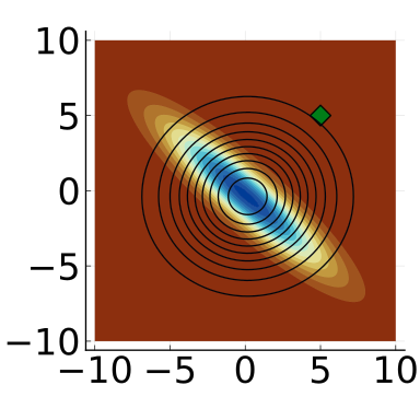
(a) $\alpha=1.0$

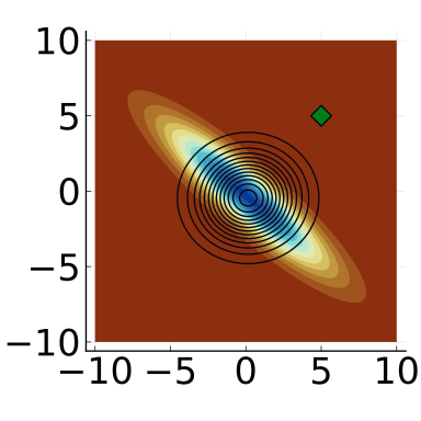
(b) $\alpha=0.5$

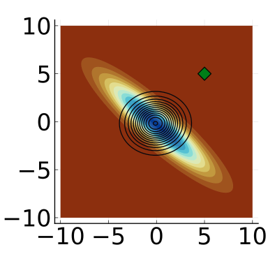
(c) $\alpha=0.25$

Figure 6: Plots of the target in color levels and the proposal in solid lines, after $k=100$ iterations for $\alpha\in\{1.0,0.5,0.25\}$. The initial mean is denoted by the green square while the initial covariance is $10I$.

We see in Fig. 6 that when $\alpha$ is high, the approximated proposals tend to cover most of the mass of the target. Lower values of $\alpha$ lead instead to proposals that are highly concentrated around the mode of the target and thus less spread which is in accordance with the observations of [66].

D.1.2 Interplay between $\alpha$ and $\tau$: speed or robustness

We now discuss the influence of $\alpha,\tau$ on the practical speed and robustness of Algorithm 2, in its non-regularized version RMM. We recall that this algorithm resorts to importance sampling to approximate the integrals involved in the computation of $\pi_{\theta}^{(\alpha)}(\Gamma)$, which creates an approximation error linked with the sample size, $N$. The influence of $\tau$ can be understood through the theory on stochastic Bregman gradient descent with fixed step-size. In particular, [47, Theorem 5.3] states that such methods converge to a neighborhood of the optimum, whose size decreases with $\tau$. On the other hand, low values of $\alpha$ amount to a concave transformation of the importance weights, which is known in the importance sampling field to lead to a higher effective sample size [61].

In order to highlight this compromise between speed and robustness, we use the RMM algorithm to approximate the target described in Eq. (61) with $\kappa=10$. We use a constant number of samples per iteration $N=500$, for $d\in\{5,10,20,40\}$. It is recommended for importance sampling procedures that the sample size grows as $\exp(d)$ to avoid weight degeneracy [16]. In our setting, $d$ increases while $N$ remains constant, thus creating approximation errors that increase with $d$.

For each dimension, we test $\alpha\in\{0.5,1.0\}$ and $\tau\in\{0.25,0.5,1.0\}$. We track the square errors $\|\bar{\mu}-\mu_{k}\|^{2}$ and $\|\bar{\Sigma}_{\kappa}-\Sigma_{k}\|_{F}^{2}$, that are averaged over $10^{3}$ independent runs.

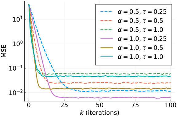
(a) MSE on the mean

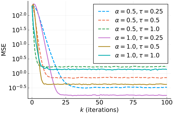
(b) MSE on the covariance

Figure 7: MSE on the mean and the covariance, averaged over $10^{3}$ runs, in dimension $d=5$.

In dimension $d=5$, all the choices of parameters lead to convergence, as shown in Fig. 7. We can notice that the lowest values of $\tau$ lead to the slowest convergence, but the values reached are lower. On the contrary, when $\tau=1.0$, the algorithm stops early at higher values.

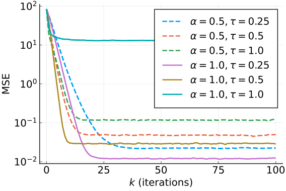
(a) MSE on the mean

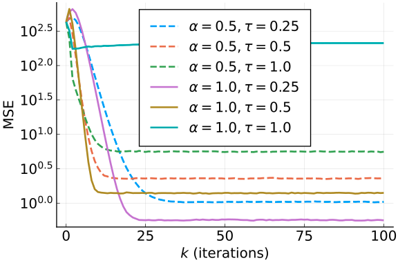
(b) MSE on the covariance

Figure 8: MSE on the mean and the covariance, averaged over $10^{3}$ runs, in dimension $d=10$.

Figure 8 shows the experiments in dimension $d=10$. We still observe the same trade-off between accuracy and speed, but we also notice that the choice $\alpha=1.0$, $\tau=1.0$ leads to failure. Indeed, it amounts to approximate $\pi(\Gamma)$ directly without using the estimates from past iterations, so the approximation errors cannot be averaged over iterations.

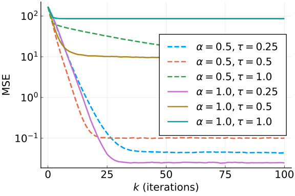
(a) MSE on the mean

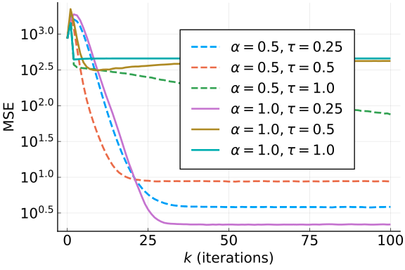
(b) MSE on the covariance

Figure 9: MSE on the mean and the covariance, averaged over $10^{3}$ runs, in dimension $d=20$.

In dimension $d=20$, we see in Fig. 9 that the only scenario reaching convergence with $\alpha=1.0$ has $\tau$ set to the lowest value. Similarly, the algorithm with the highest value of $\tau$ is only able to converge with the lowest value of $\alpha$, but with very slow convergence. This may indicate that $\alpha$ and $\tau$ both allow to average the approximation errors in Algorithm 2, which is linked to the interpretation of the relaxed moment-matching updates as barycenters, as discussed in Section 3.3.

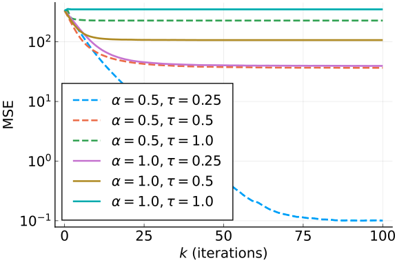
(a) MSE on the mean

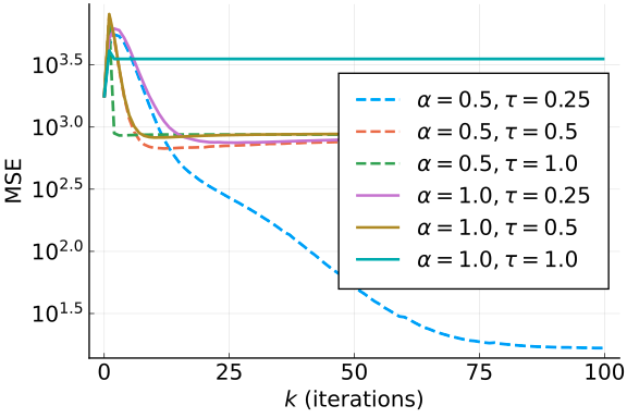
(b) MSE on the covariance

Figure 10: MSE on the mean and the covariance, averaged over $10^{3}$ runs, in dimension $d=40$.

Finally, for $d=40$, only the lowest values of $\alpha$ and $\tau$ yield a significant decrease of the MSE as shown in Fig. 10. This shows that low values of $\alpha$ and $\tau$ can counteract high approximation errors. As expected, the convergence is slower and the final MSE values are higher than in lower dimensions.

This study shows that the parameters $\alpha$ and $\tau$ should be lowered to compensate for high approximation errors possibly arising in Algorithm 2. On the contrary, when these errors are low, one can increase the values of $\tau$ to create faster algorithms.

D.1.3 Adding a regularizer: mismatch and improved behavior

Adding a regularizer $r$ is a feature of our novel method. We thus compare the PRMM and the RMM algorithm, to investigate the influence of $r$. A minimizer $\theta_{*}$ of $F_{\pi}^{(\alpha)}=f_{\pi}^{(\alpha)}+r$ is not a minimizer of $f_{\pi}^{(\alpha)}$, meaning that the regularized solutions $q_{\theta_{*}}$ are further from $\pi$, but the parameters $\theta_{*}$ have some features enforced by $r$. We now illustrate the effects of such a regularizer, showing its benefits when $\pi$ is poorly conditioned and the approximation errors are high.

We consider again the target from Eq. (61), with $\kappa=10$. For the PRMM algorithm, we set $r$ as an indicator function constraining the approximated proposal covariance matrix to be in the set $E_{\epsilon}$ of symmetric matrices whose eigenvalues are in $[\epsilon,1/\epsilon]$ for $\epsilon\in(0,1)$. The computation of the corresponding proximal step, which is here a projection, is detailed in Appendix C.

(a) $k=1$, $r\equiv 0$

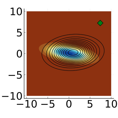
(b) $k=5$, $r\equiv 0$

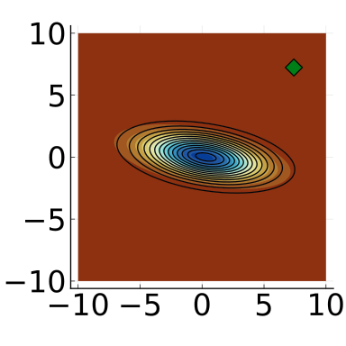
(c) $k=10$, $r\equiv 0$

(d) $k=20$, $r\equiv 0$

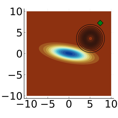
(e) $k=1$, $r=\iota_{E_{\epsilon}}$

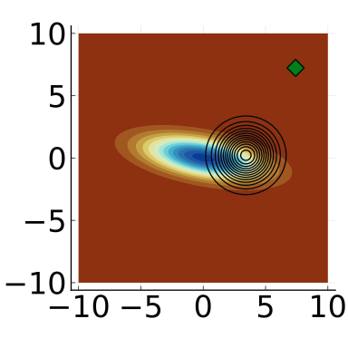
(f) $k=5$, $r=\iota_{E_{\epsilon}}$

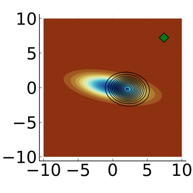
(g) $k=10$, $r=\iota_{E_{\epsilon}}$

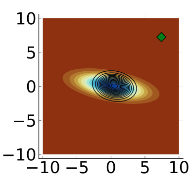
(h) $k=20$, $r=\iota_{E_{\epsilon}}$

Figure 11: One run of the RMM algorithm (top) and the PRMM algorithm (bottom), with $\epsilon=0.5$, $\alpha=0.5$, and $\tau=0.5$. The color levels mark the target, while the solid lines mark the level sets of the approximating densities after a varying number of iterations. The initial mean $\mu_{0}$ is denoted by the green square while $\Sigma_{0}=10I$.

Since our target covariance has a condition number equal to $\kappa=10$, and matrices in the constraint set $E_{\epsilon}$ have a condition number bounded above by $1/\epsilon^{2}$ with $\epsilon=0.5$, there is a mismatch $\bar{\Sigma}_{\kappa}\notin E_{\epsilon}$. This can be observed in Fig. 11. Actually, the proposal covariance are better conditioned thanks to the regularizer, which can lead to better performance in some contexts, as we illustrate in Fig. 12.

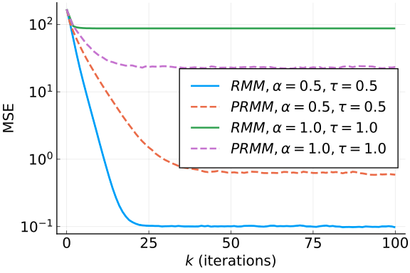
(a) MSE on the mean

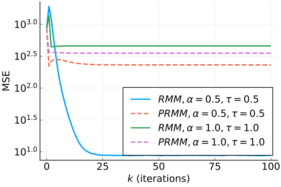
(b) MSE on the covariance

Figure 12: MSE on the mean and the covariance, averaged over $10^{3}$ runs, in dimension $d=20$. PRMM denotes the algorithms with $r=\iota_{E_{\epsilon}}$, while RMM denotes the algorithm with $r\equiv 0$.

We see that the best performance is achieved by the RMM algorithm with $\alpha=0.5$, $\tau=0.5$, while the RMM algorithm with $\alpha=1.0$ and $\tau=1.0$ achieves the worst one. These results are in accordance with the result of Section D.1.2. However, turning to the PRMM algorithm in this setting allows a performance increase from this worst case. Indeed, the PRMM algorithm achieves better performance than the RMM algorithm when $\alpha=1$, $\tau=1$, especially for the estimation of the mean. Since the target is poorly conditioned, the covariance matrices $\Sigma_{k}$, $k\in\mathbb{N}$ tend to become singular when $r\equiv 0$. This behavior is prevented by the regularization, explaining better performance in this case. Note that the PRMM algorithm cannot approximate the true covariance $\bar{\Sigma}_{\kappa}$ since $\bar{\Sigma}_{\kappa}\notin E_{\epsilon}$.

D.2 Comparison with the variational Rényi bound on a Gaussian target

Our theoretical analysis provides guidelines to choose the step-size $\tau$ for our RMM algorithm (Propositions 14 and 15) but also shows that there is no equivalent guarantees for the VRB algorithm (see Proposition 11). In particular, poorly chosen step-sizes could create unstable behaviors. We thus investigate these effects in the following by comparing our novel RMM algorithm with the VRB algorithm on Gaussian targets.

We use Gaussian target from Eq. (61), with $\kappa=10$, and $d=5$. Each algorithm is run with constant number of samples $N=500$, and constant values of the step-size $\tau$. We test values of $\alpha$ corresponding to the Hellinger distance ($\alpha=0.5$) and the KL divergence ($\alpha=1.0$). We test two different exponential families: Gaussian with full covariance, and Gaussian with diagonal covariance. For each tested value of $\tau$, $10^{3}$ runs are performed.

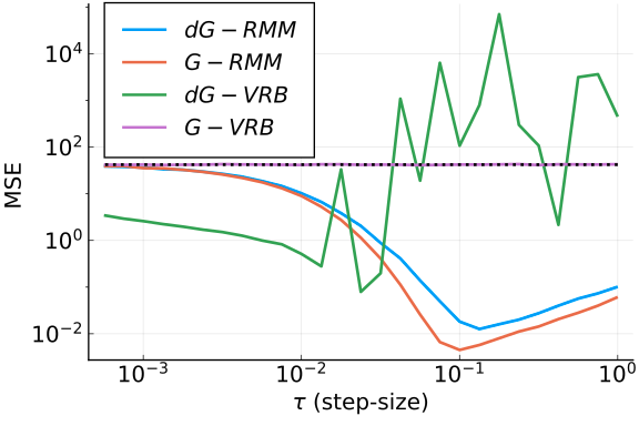
(a) MSE on the mean, $\alpha=0.5$

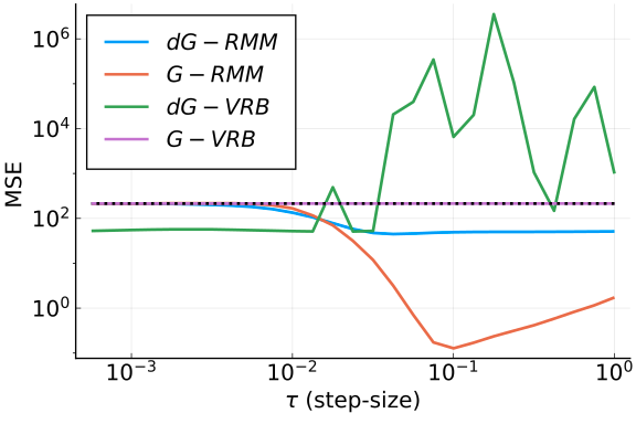
(b) MSE on the covariance, $\alpha=0.5$

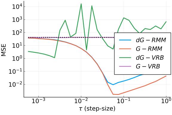
(c) MSE on the mean, $\alpha=1.0$

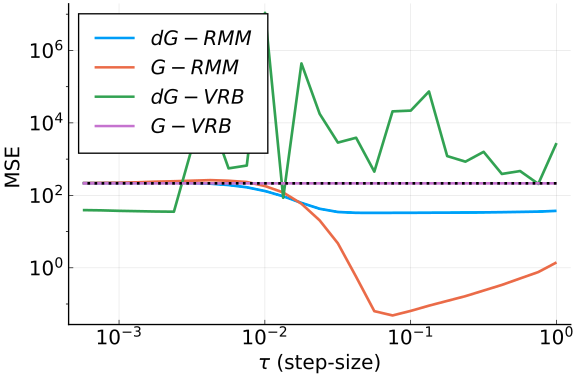
(d) MSE on the covariance, $\alpha=1.0$

Figure 13: MSE in the estimation of $\bar{\mu}$ and $\bar{\Sigma}_{\kappa}$ $(d=5)$ after $100$ iterations, against values of $\tau$. For each value of $\tau$, $10^{3}$ runs with $500$ samples per iteration are conducted. The dotted black lines represent the MSE at initialization. The prefix dG refer to the family of diagonal Gaussians, while the prefix G refers to Gaussians with full covariance.

Figure 13 shows that the VRB algorithm used with diagonal covariance in the approximation family exhibits two distinct regimes. For sufficiently low values of $\tau$, it is able to improve the estimates compared to initialization, but once $\tau$ crosses a certain threshold, the MSE reaches very high values, showing a degradation from the initialization. The VRB algorithm with full covariance in the approximation family is not able to create covariance matrices that are positive definite, hence it stops after initialization. On the contrary, our RMM algorithm does not degrade the values reached at initialization even for the worst settings of $\tau$, and reaches the lowest MSE values for properly chosen step-sizes.

This confirms that the lack of Euclidean smoothness of $f_{\pi}^{(\alpha)}$ translates numerically into a high level of instability of VRB with respect to the choice of the step-size. On the contrary, the RMM algorithm has a more stable behavior even for poorly chosen step-sizes, confirming the theoretical study of Section 5.

References

- Akyildiz and Míguez [2021] O. Akyildiz and J. Míguez. Convergence rates for optimised adaptive importance samplers. Statistic and Computing, 31(12), 2021.
- Amari [1985] S. Amari. Differential-Geometrical Methods in Statistics. Springer New York, 1985.
- Amari [1998] S. Amari. Natural gradient works efficiently in learning. Neural Computation, 10(2):251–276, 1998.
- Amari and Cichocki [2010] S. Amari and A. Cichocki. Information geometry of divergence functions. Bulletin on Polish academy of Sciences, 58(1):183–195, 2010.
- Ambrosio et al. [2005] L. Ambrosio, N. Gigli, and G. Savaré. Gradient flows: in metric spaces and in the space of probability measures. Birkhäuser, 2005.
- Aubin-Frankowski et al. [2022] P.-C. Aubin-Frankowski, A. Korba, and F. Léger. Mirror descent with relative smoothness in measure spaces, with application to Sinkhorn and EM. In Advances in Neural Information Processing Systems, volume 36, 2022.
- Bamler et al. [2017] R. Bamler, C. Zhang, M. Offred, and S. Mandt. Perturbative black box variational inference. In Advances in Neural Information Processing Systems, volume 30, 2017.
- Banerjee et al. [2008] O. Banerjee, L. E. Ghaoui, and A. d’Aspremont. Model selection through sparse maximum likelihood estimation for multivariate gaussian or binary data. Journal of Machine Learning Research, 9(15):485–516, 2008.
- Barndorff-Nielsen [2014] O. Barndorff-Nielsen. Information and Exponential Families in Statistical Theory. John Wiley & Sons, Ltd, 2014.
- Bauschke and Borwein [1997] H. Bauschke and J. Borwein. Legendre functions and the method of random Bregman projections. Journal of Convex Analysis, 4:27–67, 1997.
- Bauschke and Combettes [2011] H. Bauschke and P. Combettes. Convex Analysis and Monotone Operator Theory in Hilbert Spaces. Springer, 2011.
- Bauschke et al. [2003] H. Bauschke, J. Borwein, and P. Combettes. Bregman monotone optimization algorithms. SIAM Journal on Control and Optimization, 42(2):596–636, 2003.
- Bauschke et al. [2017] H. Bauschke, J. Bolte, and M. Teboulle. A descent lemma beyond Lipschitz gradient continuity: revisited and applications. Mathematics of Operations Research, 42(2):330–348, 2017.
- Beck and Teboulle [2003] A. Beck and M. Teboulle. Mirror descent and nonlinear projected subgradient optimization. Operations Research Letters, 31(3):167–175, 2003.
- Benfenati et al. [2020] A. Benfenati, E. Chouzenoux, and J.-C. Pesquet. Proximal approaches for matrix optimization problems: Application to robust precision matrix estimation. Signal Processing, 169, 2020.
- Bengsston et al. [2008] T. Bengsston, P. Bickel, and B. Li. Curse-of-dimensionality revisited: Collapse of the particle filter in very large scale systems, pages 316–334. Institute of Mathematical Statistics, 2008.
- Blei et al. [2017] D. Blei, A. Kucukelbir, and J. McAuliffe. Variational inference: A review for the statistician. Journal of the American Statistical Association, 112(518):859–877, 2017.
- Bolte et al. [2018] J. Bolte, S. Sabach, M. Teboulle, and Y. Vaisbourd. First order methods beyond convexity and lipschitz gradient continuity with applications to quadratic inverse problems. SIAM Journal on Optimization, 28(3):2131–2151, 2018.
- Brown [1986] L. Brown. Fundamentals of Statistical Exponential Families with Applications in Statistical Decision Theory. Institute of Mathematical Statistics, 1986.
- Bugallo et al. [2016] M. F. Bugallo, V. Elvira, and L. Martino. A new strategy for effective learning in population monte carlo sampling. In 2016 50th Asilomar Conference on Signals, Systems and Computers, pages 1540–1544. IEEE, 2016.
- Bui [2020] T. Bui. Connecting the thermodynamic variational objective and annealed importance sampling. Technical report, 2020.
- Campbell and Beronov [2019] T. Campbell and B. Beronov. Sparse variational inference: Bayesian coresets from scratch. In Advances in Neural Information Processing Systems, volume 32, 2019.
- Campbell and Li [2019] T. Campbell and X. Li. Universal boosting variational inference. In Advances in Neural Information Processing Systems, volume 32, 2019.
- Cappé et al. [2008] O. Cappé, R. Douc, A. Guillin, J. M. Marin, and C. P. Robert. Adaptive importance sampling in general mixture classes. Stat. Comput., 18:447–459, 2008.
- Carothers [2000] N. Carothers. Real Analysis. Cambridge University Press, 2000.
- Chopin and Papaspilopoulos [2020] N. Chopin and O. Papaspilopoulos. An Introduction to Sequential Monte Carlo. Springer, 2020.
- Cichocki and Amari [2010] A. Cichocki and S.-I. Amari. Families of alpha- beta- and gamma- divergences: Flexible and robust measures of similarities. Entropy, 12(6):1532–1568, 2010.
- Combettes and Pesquet [2010] P. Combettes and J.-C. Pesquet. Proximal Splitting Methods in Signal Processing, page 185–212. Springer-Verlag, New York, 2010.
- Combettes and Müller [2018] P. L. Combettes and C. L. Müller. Perspective functions: Proximal calculus and applications in high-dimensional statistics. Journal of Mathematical Analysis and Applications, 457(2):1283–1306, 2018.
- Cornuet et al. [2012] J. M. Cornuet, J. M. Marin, A. Mira, and C. P. Robert. Adaptive multiple importance sampling. Scandinavian Journal of Statistics, 39(4):798–812, December 2012.
- Csiszar [1975] I. Csiszar. -divergence geometry of probability distributions and minimization problems. The Annals of Probability, 3(1):146–158, 1975.
- Csiszár and Shields [2004] I. Csiszár and P. Shields. Information Theory and Statistics: A Tutorial. Now Foundations and Trends, 2004.
- Daudel et al. [2021a] K. Daudel, R. Douc, and F. Portier. Infinite-dimensional gradient-based descent for alpha-divergence minimisation. The Annals of Statistics, 49(4):2250–2270, 2021a.
- Daudel et al. [2021b] K. Daudel, R. Douc, and F. Roueff. Monotonic alpha-divergence minimization. https://arxiv.org/abs/2103.05684, 2021b.
- Dieng et al. [2017] A. B. Dieng, D. Tran, R. Ranganath, J. Paisley, and D. Blei. Variational inference via upper bound minimization. In Advances in Neural Information Processing Systems, volume 30, 2017.
- Domke [2020] J. Domke. Provable smoothness guarantees for black-box variational inference. In Proceedings of the 37th International Conference on Machine Learning, pages 2587–2596, 2020.
- Douc et al. [2007] R. Douc, A. Guillin, J. M. Marin, and C. P. Robert. Convergence of adaptive mixtures of importance sampling schemes. Annals of Statistics, 35:420–448, 2007.
- Durmus et al. [2019] A. Durmus, S. Majewski, and B. Miasojedow. Analysis of Langevin Monte Carlo via convex optimization. Journal of Machine Learning Research, 20(73):1–49, 2019.
- Dykstra [1985] R. L. Dykstra. An iterative procedure for obtaining -projections onto the intersection of convex sets. The Annals of Probability, 13(3):975–984, 1985.
- El Gheche et al. [2018] M. El Gheche, G. Chierchia, and J.-C. Pesquet. Proximity operators of discrete information divergences. IEEE Transactions on Information Theory, 64(2):1092–1104, 2018.
- El-Laham et al. [2019a] Y. El-Laham, V. Elvira, and M. F. Bugallo. Recursive shrinkage covariance learning in adaptive importance sampling. In Proceedings of the IEEE 8th International Workshop on Computational Advances in Multi-Sensor Adaptive Processing (CAMSAP 2018), pages 624–628, 2019a.
- El-Laham et al. [2019b] Y. El-Laham, L. Martino, V. Elvira, and M. F. Bugallo. Efficient adaptive multiple importance sampling. In Proceedings of the 27th European Signal Processing Conference (EUSIPCO 2019), pages 1–5. IEEE, 2019b.
- Elvira et al. [2019] V. Elvira, L. Martino, D. Luengo, and M. F. Bugallo. Generalized multiple importance sampling. Statistical Science, 34(1):129–155, 2019.
- Gao et al. [2020] T. Gao, S. Lu, J. Liu, and C. Chu. Randomized Bregman coordinate descent methods for non-Lipschitz optimization. https://arxiv.org/pdf/2001.05202, 2020.
- Grivel [2021] E. Grivel. Kullback-Leibler and Rényi divergence rate for Gaussian stationary ARMA processes comparison. Digital Signal Processing, 116, 2021.
- Grosse et al. [2013] R. Grosse, C. Maddison, and R. Salakhutdinov. Annealing between distributions by averaging moments. In Advances in Neural Information Processing Systems, volume 26, 2013.
- Hanzely and Richtárik [2021] F. Hanzely and P. Richtárik. Fastest rates for stochastic mirror descent methods. Computational Optimization and Applications, 79(3):717–766, 2021.
- Hastie et al. [2009] T. Hastie, R. Tibshirani, and J. Firedman. The Elements of Statistical Learning. Springer, 2009.
- Hensman et al. [2012] J. Hensman, M. Rattray, and N. D. Lawrence. Fast variational inference in the conjugate exponential family. In Advances in Neural Information Processing Systems, volume 25, 2012.
- Hernandez-Lobato et al. [2016] J. Hernandez-Lobato, Y. Li, M. Rowland, T. Bui, D. Hernandez-Lobato, and R. Turner. Black-box alpha divergence minimization. In Proceedings of The 33rd International Conference on Machine Learning (ICML 2016), volume 48, pages 1511–1520, 2016.
- Hiriart-Urruty and Lemaréchal [1993] J.-B. Hiriart-Urruty and C. Lemaréchal. Abstract Duality for Practitioners, pages 137–193. Springer, 1993.
- Hoffman et al. [2013] M. D. Hoffman, D. M. Blei, C. Wang, and J. Paisley. Stochastic variational inference. Journal of Machine Learning Research, 14(4):1303–1347, 2013.
- Honkela et al. [2010] A. Honkela, T. Raiko, M. Kuusela, M. Tornio, and J. Karhunen. Approximate Riemannian conjugate gradient learning for fixed-form variational Bayes. Journal of Machine Learning Research, 11(106):3235–3268, 2010.
- Huang et al. [2022] Y. Huang, E. Chouzenoux, and J.-C. Pesquet. Unrolled variational Bayesian algorithm for image blind deconvolution. IEEE Transactions on Image Processing, 32:430–445, 2022.
- Ionides [2008] E. L. Ionides. Truncated importance sampling. Journal of Computational and Graphical Statistics, 17(2):295–311, 2008.
- Ji et al. [2021] G. Ji, D. Sujono, and E. B. Sudderth. Marginalized stochastic natural gradients for black-box variational inference. In Proceedings of the 38th International Conference on Machine Learning (ICML 2021), volume 139, pages 4870–4881, 2021.
- Karimi et al. [2016] H. Karimi, J. Nutini, and M. W. Schmidt. Linear convergence of gradient and proximal-gradient methods under the Polyak-Łojasiewicz condition. In ECML/PKDD, 2016.
- Khan and Lin [2017] M. Khan and W. Lin. Conjugate-computation variational inference: Converting variational inference in non-conjugate models to inferences in conjugate models. In Proceedings of the 20th International Conference on Artificial Intelligence and Statistics, pages 878–887, 2017.
- Khan et al. [2016] M. Khan, R. Babanezhad, W. Lin, M. Schmidt, and M. Sugiyama. Faster stochastic variational inference using proximal-gradient methods with general divergence functions. In Proceedings of the Thirty-Second Conference on Uncertainty in Artificial Intelligence, page 319–328, 2016.
- Knoblauch et al. [2022] J. Knoblauch, J. Jewson, and T. Damoulas. An optimization-centric view on Bayes’ rule: Reviewing and generalizing variational inference. Journal of Machine Learning Research, 23(132), 2022.
- Koblents and Míguez [2013] E. Koblents and J. Míguez. A population Monte Carlo scheme with transformed weights and its application to stochastic kinetic models. Statistics and Computing, 25(2):407–425, 2013.
- Korba and Portier [2022] A. Korba and F. Portier. Adaptive importance sampling meets mirror descent : a bias-variance tradeoff. In Proceedings of The 25th International Conference on Artificial Intelligence and Statistics, volume 151, pages 11503–11527, 2022.
- Kroese et al. [2006] D. Kroese, S. Porotsky, and R. Rubinstein. The cross-entropy method for continuous multi-extremal optimization. Methodology and commputing in applied probability, 8:383–407, 2006.
- Kullback and Leibler [1951] S. Kullback and R. A. Leibler. On information and sufficiency. The Annals of Mathematical statistics, 22(1):79–86, 1951.
- Lambert et al. [2022] M. Lambert, S. Chewi, F. Bach, S. Bonnabel, and P. Rigollet. Variational inference via Wasserstein gradient flows. https://arxiv.org/abs/2112.02424, 2022.
- Li and Turner [2016] Y. Li and R. Turner. Rényi divergence variational inference. In Advances in Neural Information Processing Systems, volume 29, 2016.
- Lin et al. [2019] W. Lin, M. E. Khan, and M. Schmidt. Fast and simple natural-gradient variational inference with mixture of exponential-family approximations. In Proceedings of the 36th International Conference on Machine Learning, volume 97, pages 3992–4002, 2019.
- M. Ashok Kumar and Sason [2016] M. M. Ashok Kumar and I. Sason. Projection theorems for the Rényi divergence on -convex sets. IEEE Transactions on Information Theory, 62(9):4924–4935, 2016.
- Ma et al. [2021] Y.-A. Ma, N. S. Chatterji, X. Cheng, N. Flammarion, P. L. Bartlett, and M. I. Jordan. Is there an analog of Nesterov acceleration for gradient-based MCMC? Bernoulli, 27(3):1942–1992, 2021.
- Marin et al. [2019] J.-M. Marin, P. Pudlo, and M. Sedki. Consistency of adaptive importance sampling and recycling schemes. Bernoulli, 25(3):1977–1998, 2019.
- Marnissi et al. [2020] Y. Marnissi, E. Chouzenoux, A. Benazza-Benyahia, and J.-C. Pesquet. Majorize–minimize adapted Metropolis–Hastings algorithm. IEEE Transactions on Signal Processing, 68:2356–2369, 2020.
- Martino et al. [2014] L. Martino, V. Elvira, D. Luengo, and J. Corander. An adaptive population importance sampler. In Proceedings of the IEEE International Conference on Acoustics, Speech and Signal Processing (ICASSP 2014), pages 8038–8042. IEEE, 2014.
- Martino et al. [2018] L. Martino, V. Elvira, J. Míguez, A. Artés-Rodríguez, and P. Djurić. A comparison of clipping strategies for importance sampling. In 2018 IEEE Statistical Signal Processing Workshop (SSP), pages 558–562. IEEE, 2018.
- Masrani et al. [2021] V. Masrani, R. Brekelmans, T. Bui, F. Nielsen, A. Galstyan, G. V. Steeg, and F. Wood. q-paths: Generalizing the geometric annealing path using power means. In Proceedings of the Thirty-Seventh Conference on Uncertainty in Artificial Intelligence, volume 161, pages 1938–1947, 2021.
- Minka [2004] T. Minka. Power EP. Technical report, 2004.
- Minka [2005] T. Minka. Divergence measures and message passing. Technical report, 2005.
- Moral et al. [2006] P. D. Moral, A. Doucet, and A. Jasra. Sequential Monte Carlo samplers. J. R. Stat. Soc. Ser. B Stat. Methodol., 68(3):411–436, 2006.
- Moré and Toraldo [1989] J. Moré and G. Toraldo. Algorithms for bound contrained quadratic programming problems. Numerische Mathematik, 55(4):377–400, 1989.
- Mukkamala et al. [2020] M. Mukkamala, P. Ochs, T. Pock, and S. Sabach. Convex-concave backtracking for inertial Bregman proximal gradient algorithms in nonconvex optimization. SIAM Journal on Mathematics of Data Science, 2(3):658–682, 2020.
- Mukkamala et al. [2022] M. Mukkamala, J. Fadili, and P. Ochs. Global convergence of model function based Bregman proximal minimization algorithms. Journal on Global Optimization, 83:753–781, 2022.
- Neal [2001] R. Neal. Annealed importance sampling. Statistics and Computing, 11:125–139, 2001.
- Nielsen and Nock [2010] F. Nielsen and R. Nock. Entropies and cross-entropies of exponential families. In Proceedings of 2010 IEEE 17th International Conference on Image Processing, pages 3621–3624, 2010.
- Ormerod et al. [2017] J. Ormerod, C. You, and S. Müller. A variational Bayes approach for variable selection. Electronic Journal of Statistics, 11(2):3549–3594, 2017.
- Penot [2013] J.-P. Penot. Calculus without Derivatives. Springer, 2013.
- Ranganath et al. [2014] R. Ranganath, S. Gerrish, and D. Blei. Black box variational inference. In Proceedings of the Seventeenth International Conference on Artificial Intelligence and Statistics, volume 33, pages 814–822, 2014.
- Raskutti and Mukherjee [2015] G. Raskutti and S. Mukherjee. The information geometry of mirror descent. IEEE transactions on Information Theory, 61(3):1451–1457, 2015.
- Robert and Casella [2004] C. P. Robert and G. Casella. Monte Carlo Statistical Methods. Springer, 2004.
- Roy et al. [2022] A. Roy, L. Shen, K. Balasubramanian, and S. Ghadimi. Stochastic zeroth-order discretizations of Langevin diffusions for Bayesian inference. Bernoulli, 28(3):1810–1834, 2022.
- Rényi [1961] A. Rényi. On measures of entropy and information. In Proceedings of the Fourth Berkeley Symposium on Mathematical Statistics and Probability, volume 1, pages 547–561, 1961.
- Saha et al. [2020] A. Saha, K. Barath, and S. Kurtek. A geometric variational approach to Bayesian inference. Journal of the American Statistical Association, 115(530):822–835, 2020.
- Seeger [2005] M. Seeger. Expectation propagation for exponential families. Technical report, 2005.
- Shao et al. [2011] Y. Shao, Y. Zhou, and D. Cai. Variational inference with graph regularization for image annotation. ACM Transactions on intelligent systems and technology, 2(2):1–21, 2011.
- Teboulle [2018] M. Teboulle. A simplified view of first order methods for optimization. Mathematical programming, 170(1):67–96, 2018.
- Titsias and Lázaro-Gredilla [2015] M. Titsias and M. Lázaro-Gredilla. Local expectation gradients for black box variational inference. In Advances in Neural Information Processing Systems, volume 28, 2015.
- van Erven and Harremoes [2014] T. van Erven and P. Harremoes. Rényi divergence and Kullback-Leibler divergence. IEEE Transactions of Information Theory, 60(7):3797–3820, 2014.
- Vehtari et al. [2015] A. Vehtari, D. Simpson, A. Gelman, Y. Yao, and J. Gabry. Pareto smoothed importance sampling. https://arxiv.org/abs/1507.02646, 2015.
- Vempala and Wibosono [2019] S. Vempala and A. Wibosono. Rapid convergence of the unadjusted Langevin algorithm: Isoperimetry suffices. In Advances in Neural Information Processing Systems, volume 32, pages 8094–8106, 2019.
- Xiao [2021] X. Xiao. A unified convergence analysis of stochastic Bregman proximal gradient and extra-gradients methods. Journal of optimization theory and applications, 188(3):605–627, 2021.
- Yao and Yang [2022] R. Yao and Y. Yang. Mean field variational inference via Wasserstein gradient flow. https://arxiv.org/abs/2207.08074, 2022.
- Yuan and Lin [2007] M. Yuan and Y. Lin. Model selection and estimation in the Gaussian graphical model. Biometrika, 94(1):19–35, 2007.
- Zhang et al. [2019] C. Zhang, J. Bütepage, H. Kjellström, and S. Mandt. Advances in variational inference. IEEE Transactions on Pattern Analysis and Machine Intelligence, 41(8):2008–2026, 2019.
- Zheng et al. [2019] Y. Zheng, A. Fraysse, and T. Rodet. Efficient unsupervised variational Bayesian image reconstruction using a sparse gradient prior. Neurocomputing, 359:449–465, 2019.