IRNet: Iterative Refinement Network for
Noisy Partial Label Learning

Abstract

Partial label learning (PLL) is a typical weakly supervised learning, where each sample is associated with a set of candidate labels. The basic assumption of PLL is that the ground-truth label must reside in the candidate set. However, this assumption may not be satisfied due to the unprofessional judgment of the annotators, thus limiting the practical application of PLL. In this paper, we relax this assumption and focus on a more general problem, noisy PLL, where the ground-truth label may not exist in the candidate set. To address this challenging problem, we propose a novel framework called “Iterative Refinement Network (IRNet)”. It aims to purify the noisy samples by two key modules, i.e., noisy sample detection and label correction. Ideally, we can convert noisy PLL into traditional PLL if all noisy samples are corrected. To guarantee the performance of these modules, we start with warm-up training and exploit data augmentation to reduce prediction errors. Through theoretical analysis, we prove that IRNet is able to reduce the noise level of the dataset and eventually approximate the Bayes optimal classifier. Experimental results on multiple datasets show the effectiveness of our method. IRNet is superior to existing state-of-the-art approaches on noisy PLL. Code: https://github.com/zeroQiaoba/IRNet.

1 Introduction

Partial label learning (PLL) [1, 2] (also called ambiguous label learning [3, 4] and superset label learning [5, 6]) is a specific type of weakly supervised learning [7]. In PLL, each sample is associated with a set of candidate labels, only one of which is the ground-truth label. Due to the high monetary cost of accurately labeled data, PLL has become an active research area in many tasks, such as web mining [8], object annotation [9, 4] and ecological informatics [10].

Unlike supervised learning [11], the ground-truth label is hidden in the candidate set and invisible to PLL [12, 13], which increases the difficulty of model training. Researchers have proposed various approaches to address this problem. These methods can be roughly divided into average-based [14, 15] and identification-based methods [16, 17]. In average-based methods, each candidate label has the same probability of being the ground-truth label. They are easy to implement but may be affected by false positive labels [18, 19]. To this end, researchers introduce identification-based methods that treat the ground-truth label as a latent variable and maximize its estimated probability by the maximum margin criterion [20, 21] or the maximum likelihood criterion [18, 9]. Due to their promising results, identification-based methods have attracted increasing attention recently.

The above PLL methods rely on a fundamental assumption that the ground-truth label must reside in the candidate set. However, this assumption may not be satisfied in real-world scenarios [22, 23]. Figure 1 shows some typical examples. In online object annotation (see Figure 1(a)), different annotators assign distinct labels to the same image. However, due to the complexity of the image and the unprofessional judgment of the annotator, the ground-truth label may not be in the candidate set. Another typical application is automatic face naming (see Figure 1(b)). An image with faces is often associated with the text caption, by which we can roughly know who is in the image. However, it is hard to guarantee that all faces have corresponding names in the text caption. Therefore, we relax the assumption of PLL and focus on a more general problem, noisy PLL, where the ground-truth label may not exist in the candidate set. Due to its intractability, few works have studied this problem.

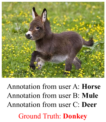
(a) online object annotation

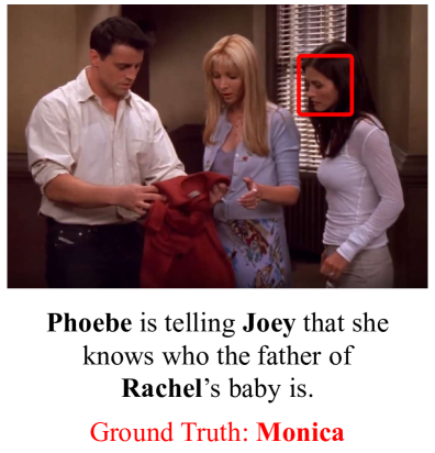
(b) automatic face naming

Figure 1: Typical applications of noisy PLL. (a) Candidate labels can be provided by crowdsourcing. However, the ground-truth label may not be in the candidate set due to the unprofessional judgments of the annotators. (b) Candidate names can be extracted from the text caption. However, there are general cases of faces without names.

The core challenge of noisy PLL is how to deal with noisy samples. To this end, we propose a novel framework called “Iterative Refinement Network (IRNet)”, which aims to purify noisy samples and reduce the noise level of the dataset. Ideally, we can approximate the performance of traditional PLL if all noisy samples are purified. IRNet is a multi-round framework consisting of two key modules, i.e., noisy sample detection and label correction. To guarantee the performance of these modules, we start with warm-up training and exploit data augmentation to further increase the reliability of prediction results. We also perform theoretical analysis and prove the feasibility of our proposed method. Qualitative and quantitative results on multiple benchmark datasets demonstrate that our IRNet outperforms currently advanced approaches under noisy conditions. The main contribution of this paper can be summarized as follows:

• Unlike traditional PLL where the ground-truth label must be in the candidate set, we focus on a seldomly discussed but vitally important task, noisy PLL, filling the gap of current works.

• To deal with noisy PLL, we design IRNet, a novel framework with theoretical guarantees.

• Experimental results on benchmark datasets show the effectiveness of our method. IRNet is superior to existing state-of-the-art methods on noisy PLL.

The remainder of this paper is organized as follows: In Section 2, we briefly review some recent works. In Section 3, we propose a novel framework for noisy PLL with theoretical guarantees. In Section 4, we introduce our experimental datasets, comparison systems and implementation details. In Section 5, we conduct experiments to demonstrate the effectiveness of our method. Finally, we conclude this paper and discuss our future work in Section 6.

2 Related Works

2.1 Non-deep Partial Label Learning

The core challenge of PLL is that the ground-truth label of each sample conceals in the candidate set. Researchers have proposed various non-deep PLL methods to disambiguate candidate labels. We roughly divide them into average-based methods and identification-based methods.

Average-based methods assume that each candidate label has an equal probability of being the ground-truth label. For parametric models, Cour et al. [14, 24] proposed to distinguish the average output of candidate and non-candidate labels. For instance-based models, Hullermeier et al. [15] estimated the ground-truth label of each sample by voting on the label information of its neighborhood. However, these average-based methods can be severely affected by false positive labels in the candidate set [18, 19].

Identification-based methods address the shortcoming of average-based methods by directly identifying the ground-truth label and maximizing its estimated probability [20]. To implement these methods, researchers have exploited various techniques, such as maximum margin [20, 21] and maximum likelihood criteria [18, 9]. For example, Nguyen et al. [20] maximized the margin between the maximum output of candidate and non-candidate labels. However, it cannot distinguish the ground-truth label from other candidate labels. To this end, Yu et al. [21] directly maximized the margin between the ground-truth label and all other labels. Unlike the maximum margin criterion, Jin et al. [18] iteratively optimized the latent ground-truth label and trainable parameters via the maximum likelihood criterion. Considering the fact that different samples and distinct candidate labels should contribute differently to the learning process, Tang et al. [25] further utilized the weight of each sample and the confidence of each candidate label to facilitate disambiguation. They exploited the model outputs to estimate the confidence of candidate labels. Differently, Zhang et al. [26, 27] and Gong et al. [28] leveraged the smoothness assumption for confidence estimation, i.e., samples that are close in feature space tend to share the same label. In addition, Liu et al. [9] maximized a mixture-based likelihood function to deal with PLL. But limited by linear models, these non-deep PLL methods are usually optimized in an inefficient manner [29].

2.2 Deep Partial Label Learning

In recent years, deep learning has greatly promoted the development of PLL. To implement deep PLL methods, researchers have proposed some training objectives compatible with stochastic optimization. For example, Lv et al. [30] introduced a self-training strategy that exploited model outputs to disambiguate candidate labels. Feng et al. [31] assumed that each incorrect label had a uniform probability of being candidate labels. Based on this assumption, they further proposed classifier- and risk-consistent algorithms with theoretical guarantees. Wen et al. [32] relaxed the data generation assumption in [31]. They introduced a family of loss functions that considered the trade-off between losses on candidate and non-candidate labels. Furthermore, Wang et al. [33] proposed PiCO, a PLL method based on contrastive learning. It utilized a prototype-based algorithm to identify the ground-truth label from the candidate set, achieving promising results on multiple benchmark datasets.

The above PLL methods are based on a fundamental assumption that the ground-truth label of each sample must reside in the candidate set [30, 31]. But due to the unprofessional judgment of the annotators, this assumption may not be satisfied in real-world scenarios.

2.3 Noisy Partial Label Learning

More recently, some researchers have noticed noisy PLL. Unlike traditional PLL, it considers a scenario where the ground-truth label may not be in the candidate set [22, 23]. Due to its intractability, few works have studied this problem. Typically, Lv et al. [23] utilized the noise-tolerant loss functions to avoid overemphasizing noisy samples in the gradient update. However, we observe that these methods cannot fully exploit the useful information in noisy samples. To learn a more discriminative classifier, we propose IRNet to purify noisy samples and reduce the noise level of the dataset. Ideally, we can convert the noisy PLL problem into the traditional PLL problem if all noisy samples are purified, resulting in better classification performance.

TABLE I: Summary of main mathematical notations.

Notations	Mathematical Meanings
$\mathcal{X},\mathcal{Y}$	feature and label space
$N,C$	number of samples and labels
$\mathcal{D}_{S},\tilde{\mathcal{D}}_{S}$	partially and fully labeled datasets
$\tilde{\mathcal{D}}_{S}^{c},\tilde{\mathcal{D}}_{S}^{n}$	clean subset and noisy subset of $\tilde{\mathcal{D}}_{S}$
$q,\eta$	ambiguity level and noise level
$x,y,\bar{y}$	feature, ground-truth label and incorrect label
$y_{j}(x)$	the $j^{th}$ element of one-hot encoded label of $x$
$S(x)$	mapping function from $x$ to its candidate set
$\omega_{1},\omega_{2}$	indicator for clean and noisy samples
$\tau,\tau_{\epsilon}$	feature and boundary for noisy sample detection
$\phi_{c},\phi_{n}$	hit accuracy for $\tilde{\mathcal{D}}_{S}^{c}$ and $\tilde{\mathcal{D}}_{S}^{n}$
$E_{\max}$	maximum number of epochs
$e_{0}$	epoch to start correction
$\mathcal{A}(x),K$	$\mathcal{A}(x)$ contains $K$ augmented samples for $x$
$h(x),h^{*}(x)$	any classify and Bayes optimal classifier
$p(y=j|x)$	posterior probability of $x$ on the label $j$
$y^{x}$	label with the highest posterior probability
$o^{x}$	label with the second highest posterior probability
$f_{j}(x)$	estimated probability of $x$ on the label $j$
$u(x),d(u)$	confidence of $x$ and its density function
$c_{*},c^{*},l$	lower bound, upper bound and ratio of $d(u)$
$L(m)$	pure level set with the boundary $m$
$\alpha,\epsilon$	two values that control the approximate gap
$\lambda_{c},\lambda_{r},\lambda_{g}$	hyper-parameters for noise-robust loss functions

3 Methodology

In this section, we first formalize the problem statement for noisy PLL. Then we discuss the motivation and introduce our proposed method in detail. Finally, we conduct theoretical analyze and prove the feasibility of IRNet.

3.1 Problem Definition

Let $\mathcal{X}$ be the input space and $\mathcal{Y}=\left\{1,2,\cdots,C\right\}$ be the label space with $C$ distinct classes. We consider a partially labeled dataset $\mathcal{D}_{S}=\{\left(x_{i},S(x_{i})\right)\}_{i=1}^{N}$ where the function $S(\cdot)$ maps each sample $x\in\mathcal{X}$ into its corresponding candidate set $S(x)\subseteq\mathcal{Y}$. The goal of PLL is to learn a multi-class classifier $f:\mathcal{X}\rightarrow\mathcal{Y}$ that minimizes the classification risk on the dataset $\mathcal{D}_{S}$. In PLL, the basic assumption is that the ground-truth label $y$ must reside in the candidate set $S(x)$. In this paper, we relax this assumption and focus on noisy PLL.

We first introduce some necessary notations. The samples that satisfy $y\in S(x)$ are called clean samples, otherwise are called noisy samples. We adopt the same generating procedure as previous works to synthesize the candidate set [30, 32]. For each sample, any incorrect label $\bar{y}\in\mathcal{Y}\backslash\{y\}$ has a probability $q$ of being an element in the candidate set. After that, each sample has a probability $\eta$ of being a noisy sample, i.e., $P\left(y\notin S(x)\right)=\eta$. In this paper, we assume that the label space is known and fixed. Both clean and noisy samples have their ground-truth labels in this space. The case where $x$ may be an out-of-distribution sample (i.e., $y\notin\mathcal{Y}$) is left for our future work [34, 35].

3.2 Observation and Motivation

In noisy PLL, the core challenge is how to deal with noisy samples. For each noisy sample, its ground-truth label $y$ conceals in the non-candidate set $\{j|j\in\mathcal{Y},j\notin S(x)\}$. A heuristic solution is to purify the noisy sample by moving $y$ from the non-candidate set to the candidate set. To this end, we need to realize two core functions: (1) detect noisy samples in the entire dataset; (2) identify the ground-truth label of each noisy sample for label correction. In this section, we conduct pilot experiments on CIFAR-10 ($q=0.3,\eta=0.3$) [36] and discuss our motivation in detail.

In the pilot experiments, we consider a fully labeled dataset $\tilde{\mathcal{D}}_{S}=\{(x_{i},y_{i},S(x_{i}))\}_{i=1}^{N}$ where the ground-truth label $y_{i}$ is associated with each sample $x_{i}$. Suppose $\omega(x_{i})\in\{\omega_{1},\omega_{2}\}$ indicates whether $x_{i}$ is clean or noisy:

$$\omega(x_{i})=\begin{cases}\omega_{1},y_{i}\in S(x_{i})\\ \omega_{2},y_{i}\notin S(x_{i}).\end{cases}$$ (1)

Based on $\omega(x_{i})$, we split the dataset $\tilde{\mathcal{D}}_{S}$ into the clean subset $\tilde{\mathcal{D}}_{S}^{c}$ and the noisy subset $\tilde{\mathcal{D}}_{S}^{n}$. In this section, $|\tilde{\mathcal{D}}_{S}^{c}|$ and $|\tilde{\mathcal{D}}_{S}^{n}|$ denote the number of samples in corresponding subsets:

$$\tilde{\mathcal{D}}_{S}^{c}=\{\left(x_{i},y_{i},S(x_{i})\right)|\omega(x_{i})=\omega_{1},1\leqslant i\leqslant N\},$$ (2)

$$\tilde{\mathcal{D}}_{S}^{n}=\{\left(x_{i},y_{i},S(x_{i})\right)|\omega(x_{i})=\omega_{2},1\leqslant i\leqslant N\}.$$ (3)

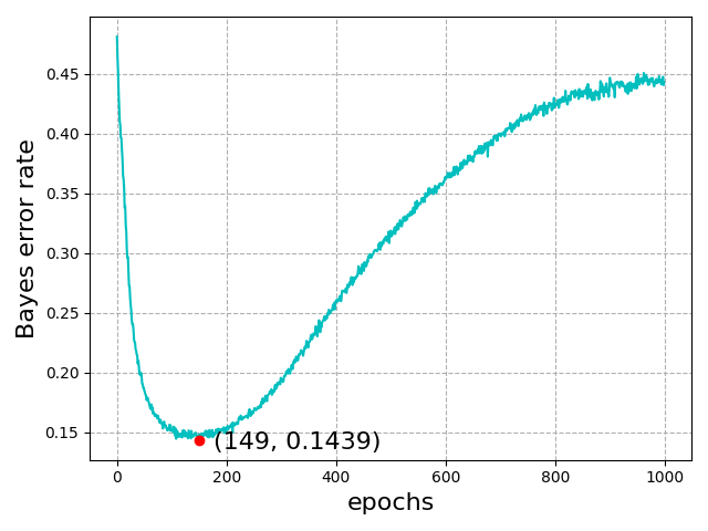
(a) Bayes error rate

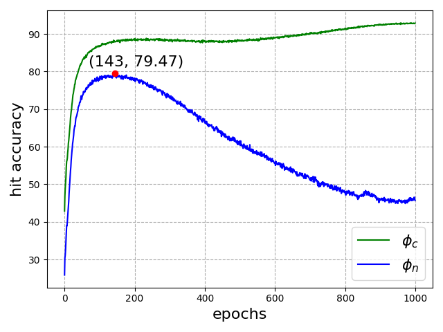
(b) hit accuracy

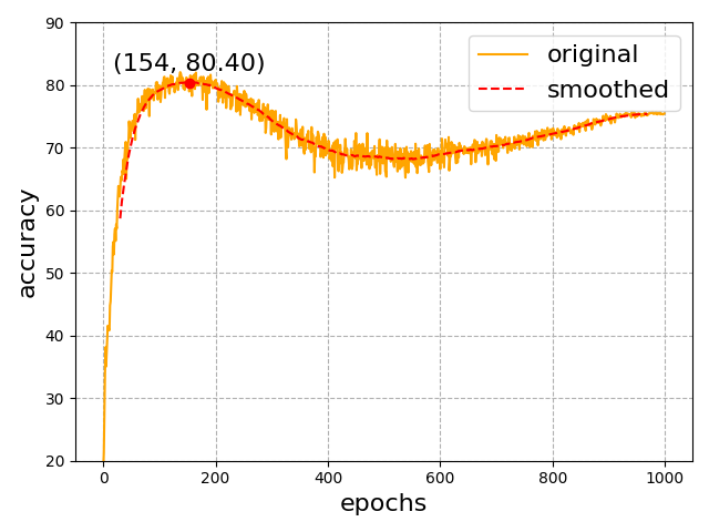
(c) validation accuracy

Figure 2: Visualization of the Bayes error rate, hit accuracy and validation accuracy on CIFAR-10 ($q=0.3,\eta=0.3$). We mark the minima in (a), the maxima in (b), and the local maxima in (c) with red dots.

3.2.1 Noisy Sample Detection

To achieve better performance on unseen data, clean samples usually contribute more than noisy samples during training [37]. Therefore, we conjecture that any metric reflecting sample contributions to the learning process can be used for noisy sample detection. In this paper, we focus on the predictive difference between the maximum output of candidate and non-candidate labels [21], a popular metric in traditional PLL [25]. This metric is calculated as follows:

$$\tau=\underset{j\in S\left(x\right)}{\max}{f_{j}\left(x\right)}-\underset{j\notin S\left(x\right)}{\max}{f_{j}\left(x\right)},$$ (4)

where $f_{j}\left(x\right)$ represents the estimated probability of the sample $x$ on the label $j$. Here, $\sum_{j=1}^{C}{f_{j}\left(x\right)=1}$.

In the pilot experiment, we attempt to verify the performance of the feature $\tau$ on noisy sample detection. This value depends on the estimated probabilities and therefore changes every epoch. To evaluate its performance, we need to train additional detectors at each epoch, which is time-consuming and computationally expensive. For convenience, we use the Bayes error rate [38]. It is easy to implement and does not require additional training process:

$$P(error|\tau)=\begin{cases}P(\omega_{2}|\tau),P(\omega_{1}|\tau)>P(\omega_{2}|\tau)\\ P(\omega_{1}|\tau),P(\omega_{1}|\tau)<P(\omega_{2}|\tau),\end{cases}$$ (5)

$$\begin{split}P(error)&=\int{P(error|\tau)p(\tau)d\tau}\\ &=\int\limits_{\mathcal{R}_{1}}{P(\omega_{2}|\tau)p(\tau)d\tau}+\int\limits_{\mathcal{R}_{2}}{P(\omega_{1}|\tau)p(\tau)d\tau}\\ &=\int\limits_{\mathcal{R}_{1}}{p(\tau|\omega_{2})P(\omega_{2})d\tau}+\int\limits_{\mathcal{R}_{2}}{p(\tau|\omega_{1})P(\omega_{1})d\tau}.\end{split}$$ (6)

Based on whether satisfying $P(\omega_{1}|\tau)>P(\omega_{2}|\tau)$, we divide the space into two regions $\mathcal{R}_{1}$ and $\mathcal{R}_{2}$. Here, $P(\omega_{1})$ and $P(\omega_{2})$ are the prior probabilities for noisy sample detection. Since we cannot obtain such priors, we set them to $P(\omega_{1})=P(\omega_{2})=0.5$. Meanwhile, we leverage histograms to approximate the class-conditional probability density functions $P(\tau|\omega_{1})$ and $P(\tau|\omega_{2})$.

Experimental results are presented in Fig. 2(a). A lower Bayes error rate means better performance. If we randomly determine whether a sample is clean or noisy, the Bayes error rate is $P(error)=0.50$. From Fig. 2(a), we observe that the Bayes error rate can reach $P(error)=0.14$, much lower than random guessing. Therefore, we can infer from $\tau$ whether a sample is more likely to be clean or noisy.

3.2.2 Label Correction

After noisy sample detection, we try to identify the ground-truth label of each noisy sample so that we can correct it by moving the predicted label into its candidate set. For the clean sample, previous works usually select the candidate label with the highest probability $\arg\max_{j\in S(x)}{f_{j}\left(x\right)}$ as the predicted label [25, 39]. For the noisy sample, the ground-truth label conceals in the non-candidate set. Naturally, we conjecture that the non-candidate label with the highest probability $\arg\max_{j\notin S(x)}{f_{j}\left(x\right)}$ can be regarded as the predicted label for the noisy sample. To verify this hypothesis, we first define an evaluation metric called hit accuracy. The calculation formula is shown as follows:

$$\phi_{c}=\frac{1}{\left|\tilde{\mathcal{D}}_{S}^{c}\right|}{\sum\nolimits_{\left(x,y,S\left(x\right)\right)\in\tilde{\mathcal{D}}_{S}^{c}}}{\mathbb{I}\left(y=\underset{j\in S(x)}{\arg\max}{f_{j}(x)}\right)},$$ (7)

$$\phi_{n}=\frac{1}{\left|\tilde{\mathcal{D}}_{S}^{n}\right|}{\sum\nolimits_{\left(x,y,S\left(x\right)\right)\in\tilde{\mathcal{D}}_{S}^{n}}}{\mathbb{I}\left(y=\underset{j\notin S(x)}{\arg\max}{f_{j}(x)}\right)},$$ (8)

where $\mathbb{I}\left(\cdot\right)$ is an indicator function. $\phi_{c}$ is the hit accuracy for the clean subset $\tilde{\mathcal{D}}_{S}^{c}$ and $\phi_{n}$ is the hit accuracy for the noisy subset $\tilde{\mathcal{D}}_{S}^{n}$. This evaluation metric measures the performance of our method on ground-truth label detection. Higher hit accuracy means better performance.

Experimental results are shown in Fig. 2(b). If we randomly select a non-candidate label as the predicted label for the noisy sample, $\phi_{n}$ is calculated as follows:

$$\begin{split}\phi_{n}&=\frac{1}{C-\mathbb{E}_{x\sim\tilde{\mathcal{D}}_{S}^{n}}\left[\left|S(x)\right|\right]}\\ &=\frac{1}{C-\left(1+\left(C-1\right)*q\right)},\end{split}$$ (9)

where $\mathbb{E}_{x\sim\tilde{\mathcal{D}}_{S}^{n}}\left[\left|S(x)\right|\right]$ denotes the expectation on the number of candidate labels. Since we conduct pilot experiments on CIFAR-10 ($q=0.3,\eta=0.3$), the hit accuracy of random guessing is $\phi_{n}=15.87$. From Fig. 2(b), we observe that our method can reach $\phi_{n}=79.47$, much higher than random guessing. These results demonstrate the effectiveness of our method on ground-truth label detection for noisy samples.

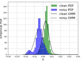
(a) 100 epoch,$P(error)$=0.15

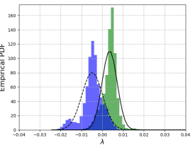
(b) 149 epoch,$P(error)$=0.14

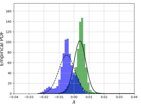
(c) 200 epoch,$P(error)$=0.15

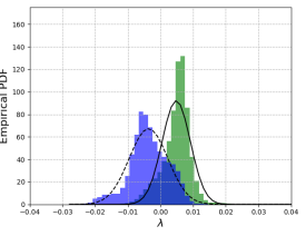
(d) 300 epoch,$P(error)$=0.19

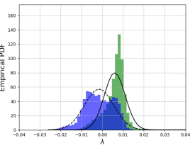
(e) 400 epoch,$P(error)$=0.26

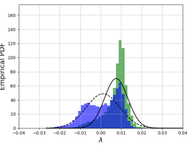
(f) 500 epoch,$P(error)$=0.32

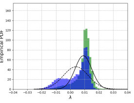
(g) 600 epoch,$P(error)$=0.36

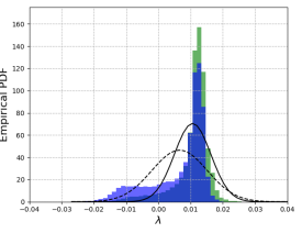
(h) 700 epoch,$P(error)$=0.40

Figure 3: Empirical PDF and estimated GMM models on CIFAR-10 ($q=0.3,\eta=0.3$) with increasing training iterations.

3.3 Iterative Refinement Network (IRNet)

Motivated by the above observations, we propose a simple yet effective framework for noisy PLL. Our method consists of two key modules, i.e., noisy sample detection and label correction. However, we find some challenges during implementation: (1) As shown in Fig. 2(a)$\sim$2(b), these modules perform poorly at the early epochs of training. Therefore, we need to find an appropriate epoch $e_{0}$. Before $e_{0}$, we start with a warm-up period with traditional PLL approaches. After $e_{0}$, we exploit IRNet for label correction. In this paper, we refer to $e_{0}$ as correction epoch; (2) Unlike pilot experiments in Section 3.2, ground-truth labels are not available in real-world scenarios. Therefore, we need to find suitable unsupervised techniques to realize these modules. In this section, we illustrate our solutions to the above challenges.

3.3.1 Choice of Correction Epoch

An appropriate $e_{0}$ is when both noisy sample detection and label correction can achieve good performance. As shown in Fig. 2(a)$\sim$2(b), the performance of these modules first increases and then decreases. Meanwhile, these modules achieve the best performance at close epochs. To find a suitable $e_{0}$, we first reveal the reasons behind these phenomena.

Previous works have demonstrated that when there is a mixture of clean and noisy samples, networks tend to fit the former before the latter [37, 40]. Based on this theory, in noisy PLL, networks start fitting clean samples so that the performance of these modules first increases. At the late epochs of training, networks tend to fit noisy samples. Since the ground-truth label of the noisy sample is not in the candidate set, networks may assign wrong predictions on the candidate set and gradually become overconfident during training. This process harms the discriminative performance of $\tau$ and leads to a decrement in $\phi_{n}$. Therefore, the epoch when networks start fitting noisy samples is a suitable $e_{0}$.

Empirically, networks cannot perform accurately on unseen data when fitting noisy samples, resulting in a drop in validation accuracy. Therefore, we conjecture that validation accuracy can be used to guide the model to find an appropriate $e_{0}$. To verify this hypothesis, we visualize the curve of validation accuracy in Fig. 2(c). We observe that it first increases and then decreases, the same trend as in Fig. 2(a)$\sim$2(b). At the late epochs of training, it gradually increases and converges to a stable value. Since $\phi_{c}$ keeps increasing during training (see Fig. 2(b)), the increment brought by clean samples is greater than the decrement brought by noisy samples, resulting in a slight improvement in validation accuracy. Therefore, we choose the epoch of the first local maximum as $e_{0}$. Experimental results demonstrate that the epoch determined by our method (the $154^{th}$ epoch) is close to the best epoch for noisy sample detection (the $149^{th}$ epoch) and label correction (the $143^{th}$ epoch). These results verify the effectiveness of our selection strategy.

3.3.2 Noisy Sample Detection

In this section, we attempt to find an appropriate approach for noisy sample detection. Since ground-truth labels are unavailable in real-world scenarios, we rely on unsupervised techniques to realize this function.

Previous works [41] usually exploit the Gaussian Mixture Model (GMM) [42], a popular unsupervised modeling technique. To verify its performance, we show the empirical PDF and estimated GMM on the feature $\tau$ for clean and noisy subsets. From Fig. 3, we observe that the Gaussian cannot accurately estimate the distribution. Hence, we need to find a more effective strategy to detect noisy samples.

From Fig. 3, we observe some interesting phenomena. As the number of training iterations increases, the range of $\tau$ is relatively fixed and most samples satisfy $\tau\in\left[-0.03,0.03\right]$. Meanwhile, samples meeting $\tau\leq-0.008$ have a high probability of being noisy samples. Inspired by the above phenomena, we determine the samples satisfying $\tau\leq-\tau_{\epsilon}$ as the noisy samples, where $\tau_{\epsilon}$ is a user-defined parameter.

3.3.3 Label Correction

After noisy sample detection, we try to identify the ground-truth label of each noisy sample for label correction. Inspired by pilot experiments in Section 3.2, we exploit the non-candidate label with the highest probability as the predicted label for the detected noisy sample. However, prediction results cannot be completely correct. To achieve better performance, we need to further reduce prediction errors.

A straightforward solution is to encourage the model’s output not to be significantly affected by natural and small input changes. This process improves the robustness of the model and increases the reliability of the prediction. Specifically, we assume that each sample has a set of augmented versions $\mathcal{A}(x)=\left\{\text{Aug}_{k}(x)|1\leqslant k\leqslant K\right\}$, where $K$ denotes the number of augmentations. $\text{Aug}_{k}(x)$ represents the $k^{th}$ augmented version for $x$. In IRNet, we select the sample satisfying the following conditions for label correction:

$$\underset{j\in S(x)}{\max}{f_{j}\left(x\right)}-\underset{j\notin S(x)}{\max}{f_{j}\left(x\right)}\leq-\tau_{\epsilon},$$ (10)

$$\underset{j\in S(x)}{\max}{f_{j}\left(z\right)}-\underset{j\notin S(x)}{\max}{f_{j}\left(z\right)}\leq-\tau_{\epsilon},\forall z\in\mathcal{A}(x),$$ (11)

$$\underset{j\notin S(x)}{\arg\max}{f_{j}\left(x\right)}=\underset{j\notin S(x)}{\arg\max}{f_{j}\left(z\right)},\forall z\in\mathcal{A}(x).$$ (12)

Therefore, we rely on stricter criteria for noisy sample detection and label correction. Besides the original sample, its augmented versions should meet additional conditions. Experimental results in Section 5.4 show that our data augmentation strategy can reduce prediction errors and improve the classification performance under noisy conditions. The pseudo-code of IRNet is summarized in Algorithm 1.

Input: PLL training set $\mathcal{D}_{S}=\{\left(x_{i},S(x_{i})\right)\}_{i=1}^{N}$, the predictive model $f$, the margin $\tau_{\epsilon}$, the number of augmentations $K$, the number of epochs $E_{\max}$, the number of iteration $T_{\max}$.

Output: The optimized model $f$.

1

2Initialize model parameters for $f$;

3for $e=1,\cdots,E_{\max}$ do

4      

5      Shuffle $\mathcal{D}_{S}$;

6      for $t=1,\cdots,T_{\max}$ do

7            

8            Sample mini-batch $\mathcal{B}_{t}=\{\left(x_{i},S(x_{i})\right)\}_{i=1}^{N_{b}}$;

9            Train the predictive model $f$ on $\mathcal{B}_{t}$;

10       end for

11      

12      Evaluate $f$ using validation accuracy and save the result in $res^{[e]}$;

13      if $e\geqslant 10$ then

14             Check the convergence condition $\sum\limits_{i=e-9}^{e}\left(res^{[i]}-res^{[i-1]}\right)<10^{-5}$;

15            if converged then

16                   $e_{0}=e$;

17                  break;

18             end if

19            

20       end if

21      

22 end for

23

24 

25

26for $e=e_{0},\cdots,E_{\max}$ do

27       Shuffle $\mathcal{D}_{S}$;

28      for $t=1,\cdots,T_{\max}$ do

29             Sample mini-batch $\mathcal{B}_{t}=\{\left(x_{i},S(x_{i})\right)\}_{i=1}^{N_{b}}$;

30            Train the predictive model $f$ on $\mathcal{B}_{t}$;

31            if $i=1,\cdots,N_{b}$ then

32                   if $x_{i}$ satisfies the conditions in Eq. 10$\sim$12 then

33                         Identify $x_{i}$ as the noisy sample;

34                        Gain the predicted label $\arg\max_{j\notin S(x_{i})}{f_{j}\left(x_{i}\right)}$ for $x_{i}$;

35                        Correct the noisy sample $x_{i}$ by moving the predicted label into its candidate set $S(x_{i})$;

36                   end if

37                  

38             end if

39            

40       end for

41      

42 end for

Algorithm 1 IRNet Algorithm

3.4 Theoretical Analysis

In this section, we conduct theoretical analysis to demonstrate the feasibility of IRNet. Our proof is inspired by previous works [43, 44] but extended to a different problem, noisy PLL. For convenience, we first introduce some necessary notations. The goal of supervised learning and noisy PLL is to learn a classifier that can make correct predictions on unseen data. Usually, we take the highest estimated probability as the predicted label $h(x)=\arg\max_{j\in\mathcal{Y}}{f_{j}\left(x\right)}$. We assume that all possible $h(x)$ form hypothesis space $\mathcal{H}$.

In supervised learning, each sample has a ground-truth label, i.e., $\tilde{\mathcal{D}}=\{(x_{i},y_{i})\}_{i=1}^{N}$. The Bayes optimal classifier $h^{*}(x)$ is the one that minimizes the following risk:

$$h^{*}(x)=\underset{h\in\mathcal{H}}{\arg\min}{\mathbb{E}_{(x,y)\sim\tilde{\mathcal{D}}}\mathbb{I}}(h(x)\neq y).$$ (13)

Unlike supervised learning, each sample is associated with a set of candidate labels in noisy PLL, i.e., $\mathcal{D}_{S}=\{\left(x_{i},S(x_{i})\right)\}_{i=1}^{N}$. The optimal classifier $f(x)$ is the one that can minimize the risk under a suitable loss function $\mathcal{L}$:

$$f(x)=\underset{h\in\mathcal{H}}{\arg\min}{\mathbb{E}_{(x,S(x))\sim\mathcal{D}_{S}}\mathcal{L}}(h(x),S(x)).$$ (14)

We assume that $\mathcal{H}$ is sufficiently complex so that $f(x)$ can approximate the Bayes optimal classifier $h^{*}(x)$. Let $y^{x}$ (or $o^{x}$) be the label with the highest (or second highest) posterior possibility, i.e., $y^{x}=\arg\max_{j\in\mathcal{Y}}\ {p(y=j|x)}$, $o^{x}=\arg\max_{j\in\mathcal{Y},j\neq y^{x}}\ p(y=j|x)$. We can measure the confidence of $x$ by the margin $u(x)=p(y^{x}|x)-p(o^{x}|x)$.

Definition 1 (Pure $(m,f,S)$-level set).

A set $L(m)=\{x|u(x)\geq m\}$ is pure for $(f,S)$ if all $x\in L(m)$ satisfy: (1) $y^{x}\in S(x)$; (2) $y^{x}=argmax_{j\in\mathcal{Y}}f_{j}(x)$.

Assumption 1 (Level set $\left(\alpha,\epsilon\right)$ consistency).

Let $I(x,z)$ be an indicator function for two samples $x$ and $z$. It is equal to 1 if the more confident sample $z$ satisfies $y^{z}\notin S(z)$, i.e., $I(x,z)=\mathbb{I}\left[y^{z}\notin S(z)|u(z)\geq u(x)\right]$. Suppose there exist two constants $\alpha>0,0<\epsilon<1$ and $S_{\text{init}}(x)$ is the initial candidate set of $x$. For any mapping function $S(\cdot)$ satisfying $|S(x)|=|S_{\text{init}}(x)|$, all $x\in\mathcal{D}_{S}$ should meet the condition:

$$\left|f_{j}(x)-p(y=j|x)\right|<\alpha\mathbb{E}_{\left(z,S(z)\right)\sim\mathcal{D}_{S}}\left[I(x,z)\right]+\frac{\epsilon}{6}.$$ (15)

Hence, the approximation error between $f_{j}(x)$ and $p(y=j|x)$ is controlled by the noise level of the dataset. Particularly, if $y^{x}$ is in $S(x)$ for all $x\in\mathcal{D}_{S}$, we will obtain a tighter constraint $\left|f_{j}(x)-p(y=j|x)\right|<\frac{\epsilon}{6}$.

Assumption 2 (Level set bounded distribution).

Let $d(u)$ be the density function of $u(x)$. Suppose there exist two constants $0<c_{*}<c^{*}$ such that the density function $d(u)$ is bounded by $c_{*}<d(u)<c^{*}$. We denote the imbalance ratio as $l=c^{*}/c_{*}$.

This assumption enforces the continuity of $d(u)$. It is crucial in the analysis since it allows borrowing information from the neighborhood to help correct noisy samples. If Assumption 1$\sim$2 hold, we can prove the following theorems:

Theorem 1 (One-round refinement).

Assume that there exists a boundary $\epsilon<m<1$ such that $L(m)$ is pure for $(f,S)$. Let $\epsilon<m_{\text{new}}<1$ be the new boundary. For all $x\in\mathcal{D}_{S}$ satisfying $max_{j\notin S(x)}f_{j}(x)-max_{j\in S(x)}f_{j}(x)\geq m_{\text{new}}-\epsilon$, we move $argmax_{j\notin S(x)}f_{j}(x)$ into $S(x)$ and move $argmin_{j\in S(x)}f_{j}(x)$ out of $S(x)$, thus generating the updated candidate set $S_{\text{new}}(x)$. After that, we train a new classifier $f^{\text{new}}(x)$ on the updated dataset $\mathcal{D}_{S_{\text{new}}}=\{\left(x_{i},S_{\text{new}}(x_{i})\right)\}_{i=1}^{N}$:

$$f^{\text{new}}(x)=\underset{h\in\mathcal{H}}{\arg\min}{\mathbb{E}_{(x,S_{\text{new}}(x))\sim\mathcal{D}_{S_{\text{new}}}}\mathcal{L}}(h(x),S_{\text{new}}(x)).$$ (16)

$L(m_{\text{new}})$ is pure for $(f^{\text{new}},S_{\text{new}})$ when $m_{\text{new}}$ satisfies:

$$(1+\frac{\epsilon}{6\alpha l})(1-m)\leq 1-m_{\text{new}}\leq(1+\frac{\epsilon}{3\alpha l})(1-m).$$ (17)

Theorem 2 (Multi-round refinement).

For an initial dataset satisfying $P(y^{x}\notin S_{\text{init}}(x))=\eta$, we assume there exists a boundary $max(2\alpha\eta+\epsilon/3,\epsilon)<m_{\text{init}}<1$ such that $L(m_{\text{init}})$ is pure for $(f^{\text{init}},S_{\text{init}})$. Repeat the one-round refinement in Theorem 1. After $R>\frac{6l\alpha}{\epsilon}log(\frac{1-\epsilon}{1-m_{\text{init}}})$ rounds with $m_{\text{end}}=\epsilon$, we obtain the final candidate set and classifier $(S_{\text{final}},f^{\text{final}})$ that satisfy:

$$P\left(y^{x}\notin S_{\text{final}}(x)\right)<c^{*}\epsilon,$$ (18)

$$P\left(\underset{j\in\mathcal{Y}}{\arg\max}{f_{j}^{\text{final}}\left(x\right)}=h^{*}(x)\right)>1-c^{*}\epsilon.$$ (19)

The above theorems demonstrate that our multi-round IRNet is able to reduce the noise level of the dataset and eventually approximate the Bayes optimal classifier. The detailed proof of these theorems is shown as follows:

Proof of Theorem 1.

Suppose there is a boundary $\epsilon<m<1$ such that $L(m)$ is pure for $(f,S)$. Based on Definition 1, all $x\in L(m)$ should satisfy: (1) $y^{x}\in S(x)$; (2) $y^{x}=argmax_{j\in\mathcal{Y}}f_{j}(x)$. Hence, $\mathbb{E}_{(z,S(z))\sim\mathcal{D}_{S}}\left[\mathbb{I}\left[y^{z}\notin S(z)|u(z)\geq u(x)\right]\right]=0$ for all $x\in L(m)$. Combined with Assumption 1, we can determine the approximation error between $f_{j}(x)$ and $p(y=j|x)$:

$$\left|f_{j}(x)-p(y=j|x)\right|<\epsilon/6<\epsilon/2.$$ (20)

Let $m_{\text{new}}$ be the new boundary satisfying $\frac{\epsilon}{6l\alpha}(1-m)<m-m_{\text{new}}<\frac{\epsilon}{3l\alpha}(1-m)$. Based on Assumption 2, we can have the following result for all $x\in L(m_{\text{new}})-L(m)$:

$$\mathbb{E}_{(z,S(z))\sim\mathcal{D}_{S}}\left[\mathbb{I}\left[y^{z}\notin S(z)|u(z)\geq u(x)\right]\right]$$

$$= P_{z}[y^{z}\notin S(z)|u(z)\geq u(x)]$$

$$= \frac{P_{z}[y^{z}\notin S(z),u(z)\geq u(x)]}{P_{z}[u(z)\geq u(x)]}$$

$$\leq \frac{P_{z}[y^{z}\notin S(z),u(z)\geq m]}{P_{z}[u(z)\geq u(x)]}+\frac{P_{z}[y^{z}\notin S(z),m\geq u(z)\geq m_{\text{new}}]}{P_{z}[u(z)\geq u(x)]}$$

$$= \frac{P_{z}[y^{z}\notin S(z),u(z)\geq m]}{P_{z}[u(z)\geq m]}\frac{P_{z}[u(z)\geq m]}{P_{z}[u(z)\geq u(x)]}$$

$$+\frac{P_{z}[y^{z}\notin S(z),m\geq u(z)\geq m_{\text{new}}]}{P_{z}[u(z)\geq u(x)]}$$

$$= \mathbb{E}_{(z,S(z))\sim\mathcal{D}_{S}}[\mathbb{I}\left[y^{z}\notin S(z)|u(z)\geq m\right]]\frac{P_{z}[u(z)\geq m]}{P_{z}[u(z)\geq u(x)]}$$

$$+\frac{P_{z}[y^{z}\notin S(z),m\geq u(z)\geq m_{\text{new}}]}{P_{z}[u(z)\geq u(x)]}$$

$$= \frac{P_{z}[y^{z}\notin S(z),m\geq u(z)\geq m_{\text{new}}]}{P_{z}[u(z)\geq u(x)]}$$

$$\leq \frac{P_{z}[m\geq u(z)\geq m_{\text{new}}]}{P_{z}[u(z)\geq m]}$$

$$\leq \frac{c^{*}(m-m_{\text{new}})}{c_{*}(1-m)}.$$ (21)

Since $m-m_{\text{new}}<\frac{\epsilon}{3l\alpha}(1-m)$, we can further relax Eq. 1 to:

$$\begin{split}&\mathbb{E}_{(z,S(z))\sim\mathcal{D}_{S}}\left[\mathbb{I}\left[y^{z}\notin S(z)|u(z)\geq u(x)\right]\right]\\ \leq&\frac{l(m-m_{\text{new}})}{1-m}\\ \leq&\frac{c^{*}}{c_{*}(1-m)}\frac{\epsilon}{3l\alpha}(1-m)\\ =&\frac{\epsilon}{3\alpha}.\end{split}$$ (22)

Then based on Assumption 1, for all $x\in L(m_{\text{new}})-L(m)$, the approximation error between $f_{j}(x)$ and $p(y=j|x)$ should satisfy:

$$\begin{split}&|f_{j}(x)-p(y=j|x)|\\ <&\alpha\mathbb{E}_{(z,S(z))\sim\mathcal{D}_{S}}\left[\mathbb{I}\left[y^{z}\notin S(z)|u(z)\geq u(x)\right]\right]+\epsilon/6\\ <&\alpha\frac{\epsilon}{3\alpha}+\frac{\epsilon}{6}=\frac{\epsilon}{2}.\end{split}$$ (23)

Combining Eq. 20 and Eq. 23, for all $x\in L(m_{\text{new}})$, we can prove that $|f_{j}(x)-p(y=j|x)|<\epsilon/2$. Then, we get:

$$\begin{split}&f_{y^{x}}(x)-f_{j\neq y^{x}}(x)\\ \geq&\left(p(y=y^{x}|x)-\frac{\epsilon}{2}\right)-\left(p(y=j|x)+\frac{\epsilon}{2}\right)\\ \geq&p(y=y^{x}|x)-p(y=j|x)-\epsilon\\ \geq&p(y=y^{x}|x)-p(y=o^{x}|x)-\epsilon\\ \geq&m_{\text{new}}-\epsilon\geq 0.\end{split}$$ (24)

It means that for all $x\in L(m_{\text{new}})$, we have $argmax_{j}f_{j}(x)=y^{x}$. If $argmax_{j}f_{j}(x)$ is not in $S(x)$ and $max_{j\notin S(x)}f_{j}(x)-max_{j\in S(x)}f_{j}(x)\geq m_{\text{new}}-\epsilon$, we can move $argmax_{j\notin S(x)}f_{j}(x)$ into $S(x)$ and move $argmin_{j\in S(x)}f_{j}(x)$ out of $S(x)$, thus generating the updated candidate set $S_{\text{new}}(x)$. After that, all $x\in L(m_{\text{new}})$ satisfy $|S_{\text{new}}(x)|=|S(x)|$ and $y^{x}\in S_{\text{new}}(x)$. Hence, we can prove that $L(m_{\text{new}})$ is pure for $(f,S_{\text{new}})$.

Then, we train a new classifier on the updated dataset $\mathcal{D}_{S_{\text{new}}}$, i.e., $f^{\text{new}}(x)=argmin_{h\in\mathcal{H}}{\mathbb{E}_{(x,S_{\text{new}}(x))\sim\mathcal{D}_{S_{\text{new}}}}\mathcal{L}}(h(x),S_{\text{new}}(x))$. Repeating the proof of Theorem 1, we can prove that all $x\in L(m_{\text{new}})$ should satisfy $|f_{j}^{\text{new}}(x)-p(y=j|x)|<\epsilon/2$. Based on Eq. 24, we have $argmax_{j}f^{\text{new}}_{j}(x)=y^{x}$. Since $y^{x}$ is already in $S^{\text{new}}(x)$, we can prove that $L(m_{\text{new}})$ is pure for $(f^{\text{new}},S_{\text{new}})$.

Proof of Theorem 2.

For an initial dataset satisfying $P(y^{x}\notin S_{\text{init}}(x))=\eta$, all $x\in\mathcal{D}_{S_{\text{init}}}$ should satisfy:

$$\mathbb{E}_{(z,S_{\text{init}}(z))\sim\mathcal{D}_{S_{\text{init}}}}\left[\mathbb{I}\left[y^{z}\notin S_{\text{init}}(z)|u(z)\geq u(x)\right]\right]=\eta.$$ (25)

Based on Assumption 1, we can determine that the approximation error between $f_{j}^{\text{init}}(x)$ and $p(y=j|x)$:

$$|f_{j}^{\text{init}}(x)-p(y=j|x)|<\alpha\eta+\frac{\epsilon}{6}.$$ (26)

Let $m_{\text{init}}$ be the initial boundary. According to Eq. 24, $L(m_{\text{init}})$ is pure only if $|f_{j}^{\text{init}}(x)-p(y=j|x)|<\frac{m_{\text{init}}}{2}$. Therefore, we choose $m_{\text{init}}$ from $max(2\alpha\eta+\frac{\epsilon}{3},\epsilon)<m_{\text{init}}<1$.

According to Theorem 1, the updated boundary $m_{\text{new}}$ should satisfy $\left(1+\frac{\epsilon}{6l\alpha}\right)(1-m)\leq 1-m_{\text{new}}$. Therefore, we need $R$ rounds of refinement to update the boundary from $m_{\text{init}}$ to $m_{\text{end}}=\epsilon$. The value of $R$ is calculated as follows:

$$\begin{split}\left(1+\frac{\epsilon}{6l\alpha}\right)^{R}\left(1-m_{\text{init}}\right)&>1-\epsilon\\ \left(1+\frac{\epsilon}{6l\alpha}\right)^{R}&>\frac{1-\epsilon}{1-m_{\text{init}}}\\ Rlog\left(1+\frac{\epsilon}{6l\alpha}\right)&>log\left(\frac{1-\epsilon}{1-m_{\text{init}}}\right).\end{split}$$ (27)

Then, we have:

$$\begin{split}R&>log\left(\frac{1-\epsilon}{1-m_{\text{init}}}\right)/log\left(1+\frac{\epsilon}{6l\alpha}\right)\\ &>log\left(\frac{1-\epsilon}{1-m_{\text{init}}}\right)/\frac{\epsilon}{6l\alpha}.\end{split}$$ (28)

After multiple rounds of refinement, we reach the final boundary $m_{\text{end}}=\epsilon$. The final candidate set $S_{\text{final}}$ and the final classifier $f^{\text{final}}$ should meet the following conditions:

$$\begin{split}P\left(y^{x}\notin S_{\text{final}}(x)\right)&\leq P(u(x)<m_{\text{end}})\\ &=P(u(x)<\epsilon)\\ &<c^{*}\epsilon,\end{split}$$ (29)

$$\begin{split}P\left(\underset{j\in\mathcal{Y}}{\arg\max}{f_{j}^{\text{final}}\left(x\right)}\neq h^{*}(x)\right)&\leq P(u(x)<m_{\text{end}})\\ &=P(u(x)<\epsilon)\\ &<c^{*}\epsilon.\end{split}$$ (30)

Therefore, we can prove that:

$$\begin{split}&P\left(\underset{j\in\mathcal{Y}}{\arg\max}{f_{j}^{\text{final}}\left(x\right)}=h^{*}(x)\right)\\ &=1-P\left(\underset{j\in\mathcal{Y}}{\arg\max}{f_{j}^{\text{final}}\left(x\right)}\neq h^{*}(x)\right)\\ &>1-c^{*}\epsilon.\end{split}$$ (31)

It should be noticed that theory is slightly different from practice. In our implementation, we correct the noisy sample by moving the predicted label into the candidate set. But to reduce the difficulty of theoretical proof, we further remove the candidate label with the lowest confidence (i.e., $\arg\min_{j\in S(x)}{f_{j}\left(x\right)}$) to keep the number of candidate labels consistent. We compare these strategies in Section 5.6. Experimental results show that this removal operation leads to a slight decrease in classification performance. Therefore, we do not exploit the removal operation in practice.

4 Experimental Databases and Setup

In this section, we first describe the benchmark datasets in our experiments. Following that, we introduce various currently advanced baselines for comparison. Finally, we provide a detailed illustration of our implementation.

4.1 Corpus Description

We conduct experiments on four popular benchmark datasets for PLL, including CIFAR-10 [36], CIFAR-100 [36], MNIST [45] and Kuzushiji-MNIST [46]. We manually corrupt these datasets into noisy partially labeled versions. To form the candidate set for clean samples, we flip incorrect labels to false positive labels with a probability $q$ and aggregate the flipped ones with the ground-truth label, in line with previous works [30, 32]. After that, each sample has a probability $\eta$ of being a noisy sample. To form the candidate set for each noisy sample, we further select a negative label from the non-candidate set, move it into the candidate set, and move the ground-truth label out of the candidate set.

In this paper, we denote the probability $q$ as the ambiguity level and the probability $\eta$ as the noise level. The ambiguity level controls the number of candidate labels and the noise level controls the percentage of noisy samples. Since CIFAR-100 has 10 times more labels than other datasets, we consider $q\in\left\{0.01,0.03,0.05\right\}$ for CIFAR-100 and $q\in\left\{0.1,0.3,0.5\right\}$ for others. On MNIST, we find that all methods can achieve high accuracy at the low noise level $\eta=0.1$. Hence, we choose more challenging conditions for this dataset. Specifically, we consider $\eta\in\left\{0.2,0.3,0.4\right\}$ for MNIST and $\eta\in\left\{0.1,0.2,0.3\right\}$ for others.

TABLE II: Inductive performance (mean$\pm$std) comparison with different PLL methods. The best performance is highlighted in bold, and the second-highest result is labeled by ^†. The column with $\Delta_{\emph{SOTA}}$ means the improvements or reductions of IRNet compared to baselines.

Dataset	$q$	$\eta$	CC	LOG	LWC	LWS	RC	PiCO	IRNet	$\Delta_{\emph{SOTA}}$
CIFAR-10	0.1	0.1	79.81$\pm$0.22	79.81$\pm$0.23	79.13$\pm$0.53	82.97$\pm$0.24	80.87$\pm$0.30	90.78$\pm$0.24†	93.44$\pm$0.21	$\uparrow$2.66
		0.2	77.06$\pm$0.18	76.44$\pm$0.50	76.15$\pm$0.46	79.46$\pm$0.09	78.22$\pm$0.23	87.27$\pm$0.11†	92.57$\pm$0.25	$\uparrow$5.30
		0.3	73.87$\pm$0.31	73.36$\pm$0.56	74.17$\pm$0.48	74.28$\pm$0.79	75.24$\pm$0.17	84.96$\pm$0.12†	92.38$\pm$0.21	$\uparrow$7.42
	0.3	0.1	74.09$\pm$0.60	73.85$\pm$0.30	77.47$\pm$0.56	80.93$\pm$0.28	79.69$\pm$0.37	89.71$\pm$0.18†	92.81$\pm$0.19	$\uparrow$3.10
		0.2	71.43$\pm$0.56	71.44$\pm$0.41	74.02$\pm$0.35	76.07$\pm$0.38	75.69$\pm$0.63	85.78$\pm$0.23†	92.18$\pm$0.18	$\uparrow$6.40
		0.3	68.08$\pm$1.12	67.17$\pm$0.75	69.10$\pm$0.59	69.70$\pm$0.72	71.01$\pm$0.54	82.25$\pm$0.32†	91.35$\pm$0.08	$\uparrow$9.10
	0.5	0.1	69.87$\pm$0.94	70.33$\pm$0.80	70.59$\pm$1.34	70.41$\pm$2.68	72.46$\pm$1.51	88.11$\pm$0.29†	91.51$\pm$0.05	$\uparrow$3.40
		0.2	59.35$\pm$0.22	59.81$\pm$0.23	57.42$\pm$1.14	58.26$\pm$0.28	59.72$\pm$0.42	82.41$\pm$0.30†	90.76$\pm$0.10	$\uparrow$8.35
		0.3	48.93$\pm$0.52	49.64$\pm$0.46	48.93$\pm$0.37	39.42$\pm$3.09	49.74$\pm$0.70	68.75$\pm$2.62†	86.19$\pm$0.41	$\uparrow$17.44
CIFAR-100	0.01	0.1	53.63$\pm$0.46	53.10$\pm$0.61	53.16$\pm$0.87	56.05$\pm$0.20	52.73$\pm$1.05	68.27$\pm$0.08†	71.17$\pm$0.14	$\uparrow$2.90
		0.2	48.84$\pm$0.19	48.97$\pm$0.17	48.64$\pm$0.33	50.66$\pm$0.59	48.59$\pm$1.04	62.24$\pm$0.31†	70.10$\pm$0.28	$\uparrow$7.86
		0.3	45.50$\pm$0.28	45.16$\pm$0.29	45.51$\pm$0.28	45.71$\pm$0.45	45.77$\pm$0.31	58.97$\pm$0.09†	68.77$\pm$0.28	$\uparrow$9.80
	0.03	0.1	51.85$\pm$0.18	51.85$\pm$0.35	51.69$\pm$0.28	53.59$\pm$0.45	52.15$\pm$0.19	67.38$\pm$0.09†	71.01$\pm$0.43	$\uparrow$3.63
		0.2	47.48$\pm$0.30	47.82$\pm$0.33	47.60$\pm$0.44	48.28$\pm$0.44	48.25$\pm$0.38	62.01$\pm$0.33†	70.15$\pm$0.17	$\uparrow$8.14
		0.3	43.37$\pm$0.42	43.43$\pm$0.30	43.39$\pm$0.18	42.20$\pm$0.49	43.92$\pm$0.37	58.64$\pm$0.28†	68.18$\pm$0.30	$\uparrow$9.54
	0.05	0.1	50.64$\pm$0.40	51.27$\pm$1.22	50.55 $\pm$0.34	45.46$\pm$0.44	46.62$\pm$0.34	67.52$\pm$0.43†	70.73$\pm$0.09	$\uparrow$3.21
		0.2	45.87$\pm$0.36	45.88$\pm$0.13	45.85$\pm$0.28	39.63$\pm$0.80	45.46$\pm$0.21	61.52$\pm$0.28†	69.33$\pm$0.51	$\uparrow$7.81
		0.3	40.84$\pm$0.47	41.20$\pm$0.60	39.83$\pm$0.30	33.60$\pm$0.64	40.31$\pm$0.55	58.18$\pm$0.65†	68.09$\pm$0.12	$\uparrow$9.91
MNIST	0.1	0.2	96.84$\pm$0.07	96.77$\pm$0.11	96.77$\pm$0.13	97.48$\pm$0.10	97.03$\pm$0.08	99.17$\pm$0.10†	99.26$\pm$0.01	$\uparrow$0.09
		0.3	96.20$\pm$0.14	96.19$\pm$0.11	96.23$\pm$0.20	96.75$\pm$0.09	96.51$\pm$0.20	99.00$\pm$0.07†	99.23$\pm$0.03	$\uparrow$0.23
		0.4	95.30$\pm$0.16	95.22$\pm$0.21	95.34$\pm$0.12	95.77$\pm$0.13	95.65$\pm$0.21	99.00$\pm$0.04†	99.21$\pm$0.01	$\uparrow$0.21
	0.3	0.2	95.83$\pm$0.25	95.75$\pm$0.16	96.08$\pm$0.22	96.86$\pm$0.07	96.42$\pm$0.13	99.07$\pm$0.07†	99.24$\pm$0.03	$\uparrow$0.17
		0.3	94.33$\pm$0.22	94.53$\pm$0.16	94.75$\pm$0.18	95.52$\pm$0.09	95.30$\pm$0.09	98.92$\pm$0.02†	99.23$\pm$0.03	$\uparrow$0.31
		0.4	91.96$\pm$0.31	92.01$\pm$0.28	92.49$\pm$0.12	93.54$\pm$0.22	93.29$\pm$0.22	98.69$\pm$0.06†	99.16$\pm$0.04	$\uparrow$0.47
	0.5	0.2	93.54$\pm$0.27	93.41$\pm$0.15	94.25$\pm$0.21	95.82$\pm$0.11	95.03$\pm$0.09	98.93$\pm$0.03†	99.18$\pm$0.07	$\uparrow$0.25
		0.3	89.43$\pm$0.45	89.54$\pm$0.23	89.69$\pm$0.48	91.38$\pm$0.35	91.59$\pm$0.47	98.70$\pm$0.05†	99.12$\pm$0.02	$\uparrow$0.42
		0.4	74.97$\pm$0.74	74.30$\pm$1.89	71.03$\pm$1.73	52.19$\pm$3.31	78.51$\pm$0.95†	76.39$\pm$1.10	98.17$\pm$1.27	$\uparrow$19.66
Kuzushiji- MNIST	0.1	0.1	88.43$\pm$0.28	88.09$\pm$0.17	88.12$\pm$0.22	89.80$\pm$0.25	88.83$\pm$0.17	97.55$\pm$0.04†	98.07$\pm$0.07	$\uparrow$0.52
		0.2	86.22$\pm$0.27	86.08$\pm$0.31	86.13$\pm$0.46	87.32$\pm$0.44	86.76$\pm$0.36	96.95$\pm$0.16†	97.96$\pm$0.03	$\uparrow$1.01
		0.3	83.82$\pm$0.15	83.60$\pm$0.36	83.82$\pm$0.24	84.79$\pm$:0.18	84.31$\pm$0.24	96.53$\pm$0.18†	97.95$\pm$0.07	$\uparrow$1.42
	0.3	0.1	85.46$\pm$0.45	85.63$\pm$0.35	86.20$\pm$0.23	87.84$\pm$0.26	87.17$\pm$0.32	97.34$\pm$0.05†	97.97$\pm$0.03	$\uparrow$0.63
		0.2	82.15$\pm$0.70	82.39$\pm$0.61	82.95$\pm$0.53	84.61$\pm$0.57	84.28$\pm$0.42	96.57$\pm$0.06†	97.96$\pm$0.09	$\uparrow$1.39
		0.3	77.34$\pm$0.65	78.06$\pm$0.49	79.16$\pm$0.42	79.79$\pm$0.65	80.79$\pm$0.49	95.34$\pm$0.34†	97.87$\pm$0.10	$\uparrow$2.53
	0.5	0.1	81.97$\pm$0.35	81.46$\pm$0.17	82.89$\pm$0.37	84.61$\pm$0.50	84.39$\pm$0.39	96.65$\pm$0.09†	97.86$\pm$0.23	$\uparrow$1.21
		0.2	75.27$\pm$0.83	74.91$\pm$0.30	76.86$\pm$0.52	77.64$\pm$2.51	78.72$\pm$0.34	95.17$\pm$0.34†	97.34$\pm$0.22	$\uparrow$2.17
		0.3	65.63$\pm$0.58	65.48$\pm$0.42	66.08$\pm$1.00	62.20$\pm$3.01	70.27$\pm$0.40	90.87$\pm$1.75†	95.84$\pm$0.34	$\uparrow$4.97

4.2 Baselines

4.2.1 PLL Methods

To evaluate the performance of IRNet, we implement the following state-of-the-art PLL methods as baselines:

CC [31] is a classifier-consistent method that leverages the cross-entropy loss function and the transition matrix to form an empirical risk estimator.

RC [31] is a risk-consistent method that exploits the importance reweighting strategy to approximate the optimal classifier. Its algorithm process is consistent with PRODEN [30] but with additional theoretical guarantees.

LOG [47] is a strong benchmark model. It exploits an upper-bound loss to improve classification performance.

LWC [32] is a leveraged weighted (LW) loss that considers the trade-off between losses on candidate and non-candidate labels. It exploits the cross-entropy loss for LW.

LWS [32] is a variant of LWC. Different from LWC, this model employs the sigmoid loss function for LW.

PiCO [33] is a contrastive-learning-based PLL method. It exploits a prototype-based disambiguation algorithm to identify the ground-truth label from the candidate set, achieving promising results under varying ambiguity levels.

4.2.2 Noisy PLL Methods

IRNet corrects the noisy sample by moving the predicted target from the non-candidate set to the candidate set. Unlike IRNet, existing noisy PLL methods rely on noise-robust loss functions and do not exploit label correction [23]. To introduce these loss functions clearly, we convert the ground-truth label $y$ into its one-hot version $y_{j}(x),j\in[1,C]$. Here, $y_{j}(x)$ is equal to 1 if $j=y$, and 0 otherwise.

Mean Absolute Error (MAE) is bounded and symmetric. Previous works have demonstrated that this loss function is robust to label noise [48]:

$$\mathcal{L}_{\text{MAE}}=-\sum\limits_{j=1}^{C}\lVert y_{j}(x)-f_{j}(x)\rVert_{1}.$$ (32)

Mean Square Error (MSE) is bounded but not symmetric. Same with MAE, it is robust to label noise [48]:

$$\mathcal{L}_{\text{MSE}}=-\sum\limits_{j=1}^{C}\lVert y_{j}(x)-f_{j}(x)\rVert_{2}^{2}.$$ (33)

Symmetric Cross Entropy (SCE) combines Reverse Cross Entropy (RCE) with Categorical Cross Entropy (CCE) via two hyper-parameters $\lambda_{c}$ and $\lambda_{r}$ [49]. This loss function exploits the benefits of the noise-robustness provided by RCE and the implicit weighting scheme of CCE:

$$\mathcal{L}_{\text{CCE}}=-\sum\limits_{j=1}^{C}y_{j}(x)\log f_{j}(x),$$ (34)

$$\mathcal{L}_{\text{RCE}}=-\sum\limits_{j=1}^{C}f_{j}(x)\log y_{j}(x),$$ (35)

$$\mathcal{L}_{\text{SCE}}=\lambda_{c}\mathcal{L}_{\text{CCE}}+\lambda_{r}\mathcal{L}_{\text{RCE}}.$$ (36)

Generalized Cross Entropy (GCE) [50] adopts the negative Box-Cox transformation and utilizes a hyper-parameter $\lambda_{g}$ to balance MAE and CCE:

$$\mathcal{L}_{\text{GCE}}=\sum\limits_{j=1}^{C}y_{j}(x)\left(\frac{1-f_{j}(x)^{\lambda_{g}}}{\lambda_{g}}\right).$$ (37)

4.3 Implementation Details

In this paper, we propose an effective and flexible IRNet, which can be integrated with existing PLL methods. Since PiCO [33] has demonstrated its disambiguation performance in PLL, we integrate IRNet with PiCO to deal with noisy PLL. For PiCO, we utilize the same experimental setup as the original paper to eliminate its effects on the final results. There are mainly two user-specific parameters in IRNet, i.e., the margin $\tau_{\epsilon}$ and the number of augmentations $K$. We select $\tau_{\epsilon}$ from $\{0.0001,0.001,0.002,0.004,0.008,0.016\}$ and $K$ from $\{1,2\}$. To optimize all trainable parameters, we leverage the SGD optimizer and set the maximum number of epochs to $E_{\max}=1000$. We set the initial learning rate to $0.01$ and adjust it using the cosine scheduler. Train/test splits are provided in our experimental datasets. Following previous works [32, 33], we separate a clean validation set from the training set for hyper-parameter tuning. Then we transform the validation set back to its partially labeled version and merge it into the training set to obtain final classifiers. To evaluate the performance of different methods, we conduct each experiment three times with different random seeds and report the average results on the test set. All experiments are implemented with PyTorch [51] and carried out with NVIDIA Tesla V100 GPU.

For PLL baselines, we utilize the identical experimental settings according to their original papers for a fair comparison. For noisy PLL baselines, we rely on noise-robust loss functions and do not leverage label correction. There are two hyper-parameters in SCE, i.e., $\lambda_{c}$ and $\lambda_{r}$. We choose $\lambda_{c}$ from $\{0.1,1.0,6.0\}$ and $\lambda_{r}$ from $\{0.1,1.0\}$. Meanwhile, we select the user-specific parameter $\lambda_{g}$ in GCE from $\{0.5,0.6,0.7\}$.

5 Results and Discussion

In this section, we first compare the inductive and transductive performance with currently advanced approaches under varying ambiguity and noise levels. Then, we show the noise robustness of our method and reveal the impact of different augmentation strategies. Next, we conduct parameter sensitivity analysis and study the role of swapping in label correction. Finally, we visualize the latent representations to qualitatively analyze the strengths of our method.

TABLE III: Inductive performance comparison with different noisy PLL methods under varying ambiguity levels. The noise level of these datasets is fixed to $\eta=0.3$. The best performance is highlighted in bold, and the second-highest result is labeled by ^†.

Dataset	Method	$q=0.1$	$q=0.3$	$q=0.5$
CIFAR-10	MAE	89.82†	86.71†	76.42
	MSE	86.16	82.44	71.25
	SCE	89.04	84.42	59.45
	GCE	88.77	85.98	77.95†
	IRNet	92.38	91.35	86.19
MNIST	MAE	99.20†	99.10†	98.83†
	MSE	99.09	98.94	98.66
	SCE	99.14	99.01	98.60
	GCE	99.18	99.03	98.74
	IRNet	99.23	99.23	99.12
Kuzushiji- MNIST	MAE	97.38	96.52†	93.20†
	MSE	96.59	95.03	86.87
	SCE	97.30	96.09	89.30
	GCE	97.51†	96.16	92.55
	IRNet	97.95	97.87	95.84
Dataset	Method	$q=0.01$	$q=0.03$	$q=0.05$
CIFAR-100	MAE	21.97	18.27	19.26
	MSE	57.09	51.47	29.26
	SCE	40.47	27.00	18.63
	GCE	62.13†	57.95†	41.23†
	IRNet	68.77	68.18	68.09

5.1 Inductive Performance

In Table II$\sim$III, we compare the inductive performance with PLL and noisy PLL methods. Inductive results indicate the classification accuracy on the test set, i.e., test accuracy [52, 30]. Due to the small difference in performance under distinct random seeds (see Table II), we only report the average results in Table III. From these quantitative results, we have the following observations:

1. Experimental results in Table II demonstrate that IRNet succeeds over PLL methods on all datasets. Taking the results on CIFAR-10 as an example, IRNet outperforms the currently advanced approaches by 2.66%$\sim$17.44%. Taking the results on CIFAR-100 as an example, our method shows an absolute improvement of 2.90%$\sim$9.91% over baselines. The reason lies in that existing PLL methods are mainly designed for clean samples. However, noisy samples may exist due to the unprofessional judgment of the annotators. To this end, we propose IRNet to deal with noisy samples. Specifically, we correct the noisy sample by moving the predicted target from the non-candidate set to the candidate set. These results demonstrate the effectiveness of our IRNet under noisy conditions.

2. From Table II, we observe that the advantage of our method becomes more significant with increasing noise levels. Taking the results on CIFAR-10 ($q=0.3$) as an example, the performance gap rises from 3.10% to 9.10% as the noise level increases from 0.1 to 0.3. Meanwhile, the performance degradation of our method is much smaller than that of baselines. Taking the results on CIFAR-10 ($q=0.3$) as an example, as the noise level increases from 0.1 to 0.3, the performance of baselines drops by 6.01%$\sim$11.23%, while IRNet only drops by 1.46%. These results demonstrate the noise robustness of our proposed method.

3. Compared with noisy PLL baselines, we observe that IRNet also achieves better performance than these methods (see Table III). They mainly utilize the noise-tolerant loss functions to avoid overemphasizing noisy samples in the gradient update. However, these baselines cannot fully exploit the useful information in noisy samples. Differently, IRNet progressively purifies noisy samples to clean ones through multiple rounds of refinement, allowing us to leverage more clean samples to learn a more discriminative classifier. Ideally, we can convert the noisy PLL problem into the traditional PLL problem if all noisy samples are purified, resulting in better classification performance.

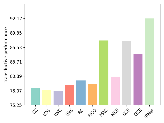
(a) CIFAR-10 ($q=0.1$)

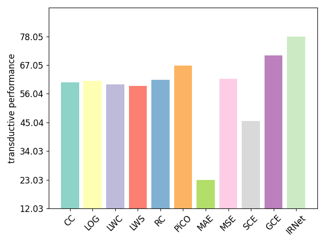
(b) CIFAR-100 ($q=0.01$)

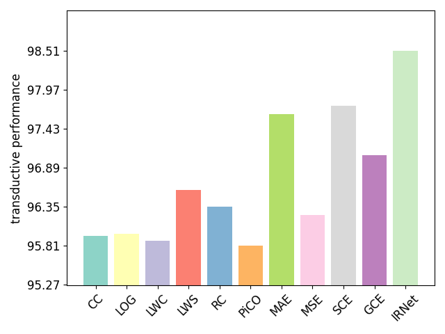
(c) MNIST ($q=0.1$)

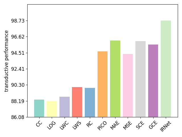
(d) Kuzushiju-MNIST ($q=0.1$)

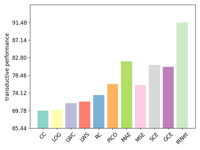
(e) CIFAR-10 ($q=0.3$)

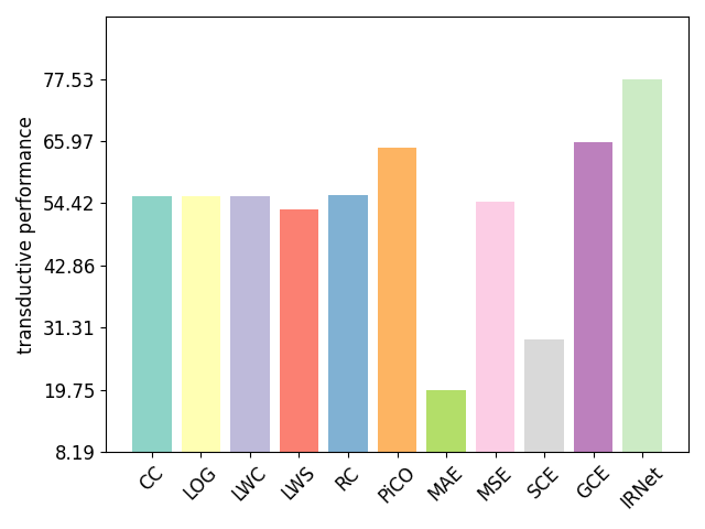
(f) CIFAR-100 ($q=0.03$)

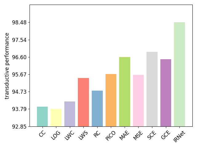
(g) MNIST ($q=0.3$)

(h) Kuzushiju-MNIST ($q=0.3$)

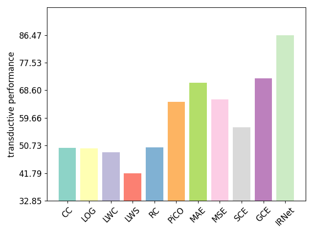
(i) CIFAR-10 ($q=0.5$)

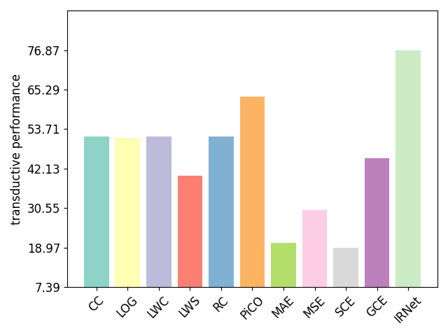
(j) CIFAR-100 ($q=0.05$)

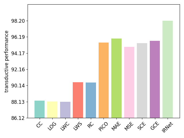
(k) MNIST ($q=0.5$)

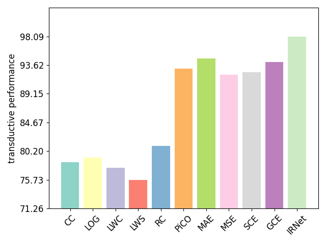
(l) Kuzushiju-MNIST ($q=0.5$)

Figure 4: Transductive performance comparison under different ambiguity levels. The noise level of these datasets is fixed to $\eta=0.3$.

5.2 Transductive Performance

Besides the inductive performance, we also evaluate the transductive performance of different approaches. Transductive results reflect the disambiguation ability on training data [52, 30]. In traditional PLL, the basic assumption is that the ground-truth label of each sample must reside in the candidate set. To evaluate the transductive performance, previous works [53] mainly determine the ground-truth label of each training sample as $\arg\max_{j\in S(x)}{f_{j}\left(x\right)}$. But this assumption is not satisfied in noisy PLL. Therefore, we predict the ground-truth label from the entire label space rather than the candidate set, i.e., $\arg\max_{j\in\mathcal{Y}}{f_{j}\left(x\right)}$.

Experimental results are shown in Fig. 4. From this figure, we observe that IRNet consistently outperforms all baselines on all datasets. These methods either ignore the presence of noisy samples or fail to exploit noisy samples effectively. Compared with these baselines, we leverage the idea of label correction to purify noisy samples. With the help of label correction, we can reduce the noise level of the dataset and achieve better transductive performance. These results also demonstrate the effectiveness of our proposed method for the noisy PLL problem.

TABLE IV: Test accuracy with and without correction under different ambiguity levels. The noise level of these datasets is fixed to $\eta=0.3$. Besides the best accuracy, we also show the test accuracy of the last epoch. The column with $\Delta$ shows the gap between the best and last accuracy.

Dataset	$q$	with correction			without correction
		Best	Last	$\Delta$	Best	Last	$\Delta$
CIFAR-10	0.1	92.38	92.22	0.16	84.96	77.94	7.02
	0.3	91.35	91.14	0.21	82.25	74.76	7.49
	0.5	86.19	85.89	0.30	68.75	66.64	2.11
CIFAR-100	0.01	68.77	68.49	0.28	58.97	54.55	4.42
	0.03	68.18	67.81	0.37	58.64	53.22	5.42
	0.05	68.09	67.75	0.34	58.18	52.81	5.37
MNIST	0.1	99.23	99.13	0.10	99.00	90.41	8.59
	0.3	99.23	99.12	0.11	98.92	88.32	10.60
	0.5	99.12	98.97	0.15	98.70	81.41	17.29
Kuzushiji- MNIST	0.1	97.95	97.81	0.14	96.53	87.11	9.42
	0.3	97.87	97.75	0.12	95.34	85.06	10.28
	0.5	95.84	95.71	0.13	90.87	78.41	12.46

5.3 Noise Robustness

The above inductive and transductive results report the best accuracy. Besides the best accuracy, the last accuracy (i.e., the test accuracy of the last epoch) reflects whether the model can prevent fitting noisy samples at the end of training. To reveal the noise robustness of our system with label correction, we further compare the last accuracy of different approaches in Table IV. In this section, we treat the system without correction as the comparison system.

• With correction: It is our method that integrates IRNet with PiCO for noisy PLL (see Section 4.3).

• Without correction: It comes from our method but omits IRNet. Therefore, this model is identical to PiCO and does not exploit label correction.

Table IV shows the performance gap between the best and last accuracy. From this table, we observe that the system with correction can obtain similar best and last results in the presence of label noise. Taking the results on MNIST as an example, the performance gap of the comparison system is 8.59%$\sim$17.29%, while the performance gap of our method is only 0.10%$\sim$0.15%. Therefore, our label correction strategy can improve the noise robustness of existing PLL systems.

Fig. 5 presents the curves of noise level and test accuracy. Without correction, the model fits noisy samples in the learning process and causes performance degradation on the test set. Differently, our method can reduce the noise level of the dataset (see Fig. 5(a)), thereby improving the test accuracy under noise conditions (see Fig. 5(b)). Meanwhile, based on theoretical analysis, the boundary $m$ should decrease exponentially in each round and eventually converge to a stable value $m_{\text{end}}$. Since $m$ is related to the noise level of the dataset $\eta$, $\eta$ should also decrease exponentially. Interestingly, we observe a similar phenomenon in Fig. 5(a). These results prove the reliability of our theoretical analysis.

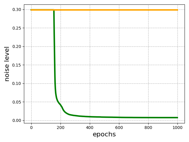
(a) noise level on training data

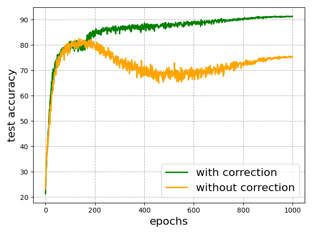
(b) test accuracy

Figure 5: Performance comparison on CIFAR-10 ($q=0.3,\eta=0.3$) with and without correction.

5.4 Importance of Augmentation

IRNet utilizes data augmentation to reduce prediction errors in noisy sample detection and label correction. To reveal the importance of data augmentation, we compare the performance of different combinations of weak (i.e., SimAugment [54]) and strong (i.e., RandAugment [55]) augmentations. Experimental results are shown in Table V.

From Table V, we observe that data augmentation can improve classification performance. Taking the results on CIFAR-10 as an example, the system with data augmentation outperforms the system without data augmentation by 0.50%$\sim$1.90%. With the help of data augmentation, we can leverage stricter criteria to select noisy samples, thereby increasing the reliability of predictions. These results demonstrate the importance of data augmentation on noisy PLL.

Meanwhile, we investigate the impact of different augmentation strategies. Experimental results in Table V show that weak augmentation can achieve better performance than strong augmentation. This phenomenon indicates that strong augmentation may not preserve all necessary information for classification. More notably, increasing the number of augmentations does not always lead to better performance. More augmentations make the selection of noisy samples more stringent and the prediction results more credible. However, some noisy samples may not be corrected due to these strict rules. Therefore, there is a trade-off between them. Strict rules lead to some noisy samples not being corrected, while loose rules lead to some clean samples being erroneously corrected. Therefore, we need to find an appropriate augmentation strategy for IRNet.

In Table VI, we further compare the complexity of different strategies. Data augmentation requires additional feedforward processing on augmented samples, resulting in more computational cost and training time. Since feedforward processing does not change the model architecture, the number of parameters remains the same. Considering the fact that increasing the number of augmentations does not always lead to better performance (see Table V), we use one weak augmentation to speed up the training process and reduce the prediction errors under noisy conditions.

TABLE V: Test accuracy of different augmentation strategies under varying ambiguity levels. The noise level of these datasets is fixed to $\eta=0.3$. In this table, #W denotes the number of weak augmentations and #S denotes the number of strong augmentations.

Dataset	#W	#S	$q=0.1$	$q=0.3$	$q=0.5$
CIFAR-10	0	0	90.78	89.87	86.51
	0	1	91.43	90.30	85.44
	1	0	92.38	91.35	86.19
	0	2	90.76	89.32	84.93
	1	1	92.26	91.32	85.94
	2	0	92.68	91.49	87.01
Dataset	#W	#S	$q=0.01$	$q=0.03$	$q=0.05$
CIFAR-100	0	0	65.40	63.93	62.88
	0	1	67.03	65.63	65.70
	1	0	68.77	68.18	68.09
	0	2	61.70	59.58	58.94
	1	1	66.32	65.13	63.46
	2	0	69.44	68.03	66.90

TABLE VI: Complexity comparison of different augmentation strategies on CIFAR-10. This table compares the MACs, number of parameters, training time per sample and GPU memory usage.

#W+#S	MACs (G)	Parameters (M)	Training Time (ms)	GPU Memory (GB)
0	1.11	23.01	1.08	3.39
1	1.67	23.01	1.18	4.05
2	2.23	23.01	1.25	4.85

5.5 Parameter Sensitivity

IRNet mainly contains two hyper-parameters, i.e., the correction epoch $e_{0}$ and the margin $\tau_{\epsilon}$. We automatically determine $e_{0}$ and manually select $\tau_{\epsilon}$. In this section, we conduct parameter sensitivity analysis to reveal the impact of these hyper-parameters. Experimental results are shown in Fig. 6.

From Fig. 6, we observe that IRNet performs poorly when $\tau_{\epsilon}$ is too large or too small. A large $\tau_{\epsilon}$ makes the selection of noisy samples strict but causes some noisy samples not to be corrected. A small $\tau_{\epsilon}$ reduces the requirement for noisy samples but causes some clean samples to be erroneously corrected. Therefore, a suitable $\tau_{\epsilon}$ can improve classification performance under noisy conditions.

Then we analyze the influence of $e_{0}$ under the optimal $\tau_{\epsilon}$. In Fig. 6(b) and Fig. 6(d), the automatically determined $e_{0}$ is 154 and 140, respectively. We also compare with $e_{0}$ in $\{1,100,200,300,400,500\}$. The performance of IRNet depends on two key modules: noisy sample detection and label correction. Since these modules perform poorly at the early or late epochs, the classification performance first increases and then decreases with increasing $e_{0}$. More notably, our automatic selection strategy can achieve competitive performance with less manual effort. These results verify the effectiveness of our selection strategy.

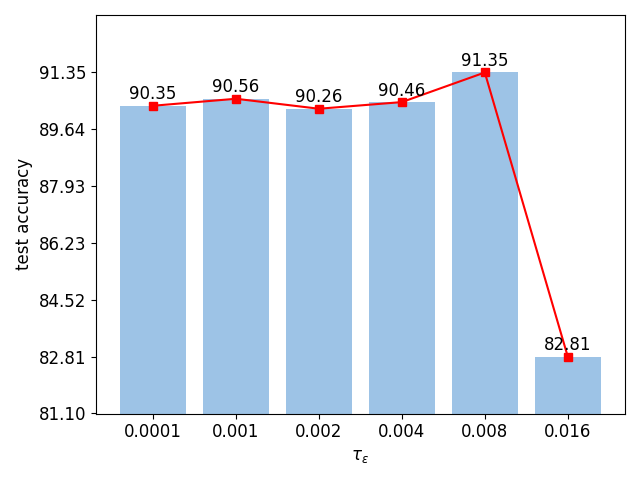
(a) $\tau_{\epsilon}$ on CIFAR-10

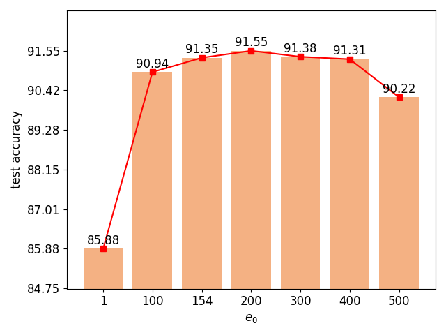
(b) $e_{0}$ on CIFAR-10 ($\tau_{\epsilon}$=0.008)

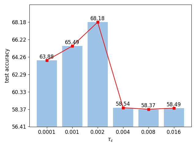
(c) $\tau_{\epsilon}$ on CIFAR-100

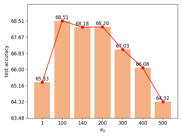
(d) $e_{0}$ on CIFAR-100 ($\tau_{\epsilon}$=0.002)

Figure 6: Parameter sensitivity analysis on CIFAR-10 ($q=0.3$) and CIFAR-100 ($q=0.03$). The noise level of these datasets is fixed to $\eta=0.3$.

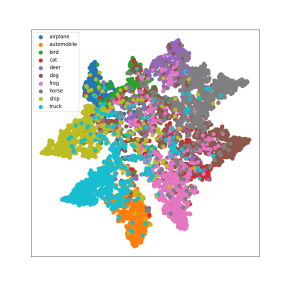
(a) LOG

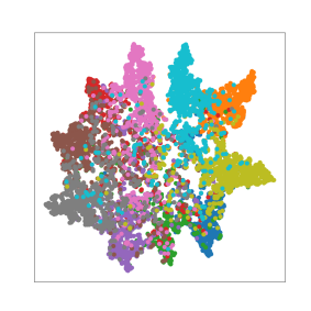
(b) RC

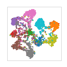
(c) PiCO

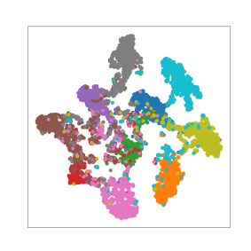
(d) MSE

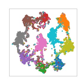
(e) SCE

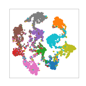
(f) GCE

(g) MAE

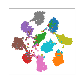
(h) IRNet

Figure 7: T-SNE visualization results of different methods on the CIFAR-10 test set ($q=0.3,\eta=0.3$).

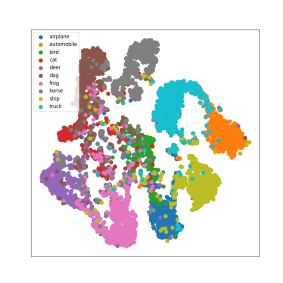
(a) 100 epoch

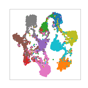
(b) 200 epoch

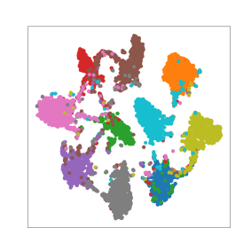
(c) 500 epoch

(d) 910 epoch

Figure 8: T-SNE visualization results of IRNet on the CIFAR-10 test set ($q=0.3,\eta=0.3$) with increasing training epochs.

5.6 Role of Swapping

In this paper, we correct the noisy sample by moving the predicted target into the candidate set. This process leads to an increase in the number of candidate labels $|S(x)|$. Previous works have demonstrated that large $|S(x)|$ may increase the difficulty of model optimization, resulting in a decrease in classification performance [31]. To keep $|S(x)|$ consistent, a heuristic solution is to further move out the candidate label with the lowest confidence (i.e., $\bar{y}=\arg\min_{j\in S(x)}{f_{j}\left(x\right)}$). To sum up, for each noisy sample, we move the predicted target into $S(x)$ and move $\bar{y}$ out of $S(x)$. We call this strategy swapping. To investigate its role on noisy PLL, we conduct additional experiments in Table VII. The system without swapping is identical to IRNet.

Experimental results in Table VII show that the swapping operation does not improve the classification performance. Taking the results on CIFAR-10 as an example, the system with swapping performs slightly worse than the system without swapping by 0.70%$\sim$2.04%. For noisy samples, the swapping operation can keep the number of candidate labels consistent by moving $\bar{y}$ out of $S(x)$. However, prediction results of IRNet are not completely correct. Due to wrong predictions, it may also move the ground-truth label out of $S(x)$ for clean samples. Therefore, we do not exploit the swapping operation in this paper.

5.7 Visualization of Embedding Space

Besides quantitative results, we also conduct qualitative analysis to show the strengths of our method. We exploit t-distributed stochastic neighbor embedding (t-SNE) [56], a tool widely utilized for high-dimensional data visualization. Figure 7 presents the visualization results of different methods. From this figure, we observe that our IRNet can effectively disentangle the latent representation and reveal the underlying class distribution. In Figure 8, we further visualize the latent features of IRNet with increasing training epochs. From this figure, we observe that the separation among classes becomes clear during training. These results also show the effectiveness of our method for noisy PLL.

TABLE VII: Test accuracy with and without swapping under varying ambiguity levels. The noise level of these datasets is fixed to $\eta=0.3$.

Dataset	$q$	with swapping	without swapping
CIFAR-10	0.1	91.48	92.38
	0.3	90.65	91.35
	0.5	84.15	86.19
CIFAR-100	0.01	67.62	68.77
	0.03	67.57	68.18
	0.05	67.19	68.09

6 Conclusions

In this paper, we study a seldomly discussed but vitally important task, noisy PLL. It relaxes the basic assumption of PLL and allows ground-truth labels of some samples are not in their candidate sets. To address this challenging task, we propose a novel framework, IRNet. Our method can purify noisy samples and reduce the noise level of the dataset. Through quantitative and qualitative analysis, we demonstrate that our IRNet outperforms currently advanced approaches in both inductive and transductive performance. Meanwhile, we verify the noise robustness of our method and reveal the importance of data augmentation. We also conduct parameter sensitivity analysis and present the impact of different hyper-parameters.

This paper focuses on the scenario where both clean and noisy samples have their ground-truth labels in a predefined label space. In the future, we will explore some challenging scenarios. For example, there are out-of-distribution samples in the dataset, and the ground-truth labels of these samples are outside the label space.

Zheng Lian received the B.S. degree from the Beijing University of Posts and Telecommunications, Beijing, China, in 2016. And he received the Ph.D degree from the Institute of Automation, Chinese Academy of Sciences, Beijing, China, in 2021. He is currently an Assistant Professor at National Laboratory of Pattern Recognition, Institute of Automation, Chinese Academy of Sciences, Beijing, China. His current research interests include affective computing, noisy label learning and partial label learning.

Mingyu Xu received the B.S. degree from Peking University, Beijing, China, in 2021. He is currently working toward the M.S. degree with the Institute of Automation, China Academy of Sciences, Beijing, China. His current research interests include uncertainty learning and partial label learning.

Lan Chen received the B.S. degree from the China University of Petroleum, Beijing, China, in 2016. And she received the Ph.D degree from the Institute of Automation, Chinese Academy of Sciences, Beijing, China, in 2022. Her current research interests include noisy label learning and image processing.

Licai Sun received the B.S. degree from Beijing Forestry University, Beijing, China, in 2016, and the M.S. degree from University of Chinese Academy of Sciences, Beijing, China, in 2019. He is currently working toward the Ph.D degree with the School of Artificial Intelligence, University of Chinese Academy of Sciences, Beijing, China. His current research interests include affective computing, deep learning and multimodal representation learning.

Bin Liu received his the B.S. degree and the M.S. degree from Beijing institute of technology, Beijing, China, in 2007 and 2009 respectively. He received Ph.D. degree from the National Laboratory of Pattern Recognition, Institute of Automation, Chinese Academy of Sciences, Beijing, China, in 2015. He is currently an Associate Professor in the National Laboratory of Pattern Recognition, Institute of Automation, Chinese Academy of Sciences, Beijing, China. His current research interests include affective computing and audio signal processing.

Jianhua Tao received the Ph.D. degree from Tsinghua University, Beijing, China, in 2001, and the M.S. degree from Nanjing University, Nanjing, China, in 1996. He is currently a Professor with Department of Automation, Tsinghua University, Beijing, China. He has authored or coauthored more than eighty papers on major journals and proceedings. His current research interests include speech recognition, speech synthesis and coding methods, human–computer interaction, multimedia information processing, and pattern recognition. He is the Chair or Program Committee Member for several major conferences, including ICPR, ACII, ICMI, ISCSLP, etc. He is also the Steering Committee Member for the IEEE Transactions on Affective Computing, an Associate Editor for Journal on Multimodal User Interface and International Journal on Synthetic Emotions, and the Deputy Editor-in-Chief for Chinese Journal of Phonetics.

References

- [1] Y. Yan and Y. Guo, “Partial label learning with batch label correction,” in Proceedings of the AAAI Conference on Artificial Intelligence, 2020, pp. 6575–6582.
- [2] F. Zhang, L. Feng, B. Han, T. Liu, G. Niu, T. Qin, and M. Sugiyama, “Exploiting class activation value for partial-label learning,” in Proceedings of the International Conference on Learning Representations, 2021, pp. 1–17.
- [3] Y.-C. Chen, V. M. Patel, R. Chellappa, and P. J. Phillips, “Ambiguously labeled learning using dictionaries,” IEEE Transactions on Information Forensics and Security, vol. 9, no. 12, pp. 2076–2088, 2014.
- [4] C.-H. Chen, V. M. Patel, and R. Chellappa, “Learning from ambiguously labeled face images,” IEEE Transactions on Pattern Analysis and Machine Intelligence, vol. 40, no. 7, pp. 1653–1667, 2017.
- [5] L. Liu and T. Dietterich, “Learnability of the superset label learning problem,” in Proceedings of the International Conference on Machine Learning, 2014, pp. 1629–1637.
- [6] E. Hüllermeier and W. Cheng, “Superset learning based on generalized loss minimization,” in Joint European Conference on Machine Learning and Knowledge Discovery in Databases, 2015, pp. 260–275.
- [7] Z.-H. Zhou, “A brief introduction to weakly supervised learning,” National Science Review, vol. 5, no. 1, pp. 44–53, 2018.
- [8] M. J. Huiskes and M. S. Lew, “The mir flickr retrieval evaluation,” in Proceedings of the 1st ACM International Conference on Multimedia Information Retrieval, 2008, pp. 39–43.
- [9] L.-P. Liu and T. G. Dietterich, “A conditional multinomial mixture model for superset label learning,” in Proceedings of the 25th International Conference on Neural Information Processing Systems, 2012, pp. 548–556.
- [10] F. Briggs, X. Z. Fern, and R. Raich, “Rank-loss support instance machines for miml instance annotation,” in Proceedings of the 18th ACM SIGKDD International Conference on Knowledge Discovery and Data Mining, 2012, pp. 534–542.
- [11] R. Caruana and A. Niculescu-Mizil, “An empirical comparison of supervised learning algorithms,” in Proceedings of the International Conference on Machine Learning, 2006, pp. 161–168.
- [12] L. Feng and B. An, “Leveraging latent label distributions for partial label learning.” in Proceedings of the International Joint Conference on Artificial Intelligence, 2018, pp. 2107–2113.
- [13] N. Xu, C. Qiao, X. Geng, and M.-L. Zhang, “Instance-dependent partial label learning,” in Proceedings of the Advances in Neural Information Processing Systems, 2021, pp. 27 119–27 130.
- [14] T. Cour, B. Sapp, C. Jordan, and B. Taskar, “Learning from ambiguously labeled images,” in IEEE Conference on Computer Vision and Pattern Recognition, 2009, pp. 919–926.
- [15] E. Hüllermeier and J. Beringer, “Learning from ambiguously labeled examples,” Intelligent Data Analysis, vol. 10, no. 5, pp. 419–439, 2006.
- [16] D.-D. Wu, D.-B. Wang, and M.-L. Zhang, “Revisiting consistency regularization for deep partial label learning,” in Proceedings of the International Conference on Machine Learning, 2022, pp. 24 212–24 225.
- [17] S.-Y. Xia, J. Lv, N. Xu, and X. Geng, “Ambiguity-induced contrastive learning for instance-dependent partial label learning,” in Proceedings of the Thirty-First International Joint Conference on Artificial Intelligence, IJCAI, 2022, pp. 3615–3621.
- [18] R. Jin and Z. Ghahramani, “Learning with multiple labels,” in Proceedings of the 15th International Conference on Neural Information Processing Systems, 2002, pp. 921–928.
- [19] W. Wang and M.-L. Zhang, “Partial label learning with discrimination augmentation,” in Proceedings of the 28th ACM SIGKDD International Conference on Knowledge Discovery and Data Mining, 2022, pp. 1920–1928.
- [20] N. Nguyen and R. Caruana, “Classification with partial labels,” in Proceedings of the 14th ACM SIGKDD International Conference on Knowledge Discovery and Data Mining, 2008, pp. 551–559.
- [21] F. Yu and M.-L. Zhang, “Maximum margin partial label learning,” in Proceedings of the Asian Conference on Machine Learning, 2016, pp. 96–111.
- [22] J. Cid-Sueiro, “Proper losses for learning from partial labels,” in Proceedings of the 25th International Conference on Neural Information Processing Systems, 2012, pp. 1565–1573.
- [23] J. Lv, L. Feng, M. Xu, B. An, G. Niu, X. Geng, and M. Sugiyama, “On the robustness of average losses for partial-label learning,” arXiv preprint arXiv:2106.06152, 2021.
- [24] T. Cour, B. Sapp, and B. Taskar, “Learning from partial labels,” Journal of Machine Learning Research, vol. 12, pp. 1501–1536, 2011.
- [25] C.-Z. Tang and M.-L. Zhang, “Confidence-rated discriminative partial label learning,” in Proceedings of the Thirty-First AAAI Conference on Artificial Intelligence, 2017, pp. 2611–2617.
- [26] M.-L. Zhang and F. Yu, “Solving the partial label learning problem: An instance-based approach,” in Proceedings of the International Joint Conference on Artificial Intelligence, 2015.
- [27] M.-L. Zhang, B.-B. Zhou, and X.-Y. Liu, “Partial label learning via feature-aware disambiguation,” in Proceedings of the 22nd ACM SIGKDD International Conference on Knowledge Discovery and Data Mining, 2016, pp. 1335–1344.
- [28] C. Gong, T. Liu, Y. Tang, J. Yang, J. Yang, and D. Tao, “A regularization approach for instance-based superset label learning,” IEEE Transactions on Cybernetics, vol. 48, no. 3, pp. 967–978, 2017.
- [29] Y. Yao, J. Deng, X. Chen, C. Gong, J. Wu, and J. Yang, “Deep discriminative cnn with temporal ensembling for ambiguously-labeled image classification,” in Proceedings of the AAAI Conference on Artificial Intelligence, 2020, pp. 12 669–12 676.
- [30] J. Lv, M. Xu, L. Feng, G. Niu, X. Geng, and M. Sugiyama, “Progressive identification of true labels for partial-label learning,” in Proceedings of the International Conference on Machine Learning, 2020, pp. 6500–6510.
- [31] L. Feng, J. Lv, B. Han, M. Xu, G. Niu, X. Geng, B. An, and M. Sugiyama, “Provably consistent partial-label learning,” in Proceedings of the Advances in Neural Information Processing Systems, 2020, pp. 10 948–10 960.
- [32] H. Wen, J. Cui, H. Hang, J. Liu, Y. Wang, and Z. Lin, “Leveraged weighted loss for partial label learning,” in Proceedings of the International Conference on Machine Learning. PMLR, 2021, pp. 11 091–11 100.
- [33] H. Wang, R. Xiao, Y. Li, L. Feng, G. Niu, G. Chen, and J. Zhao, “Pico: Contrastive label disambiguation for partial label learning,” in Proceedings of the International Conference on Learning Representations, 2022, pp. 1–18.
- [34] D. Hendrycks and K. Gimpel, “A baseline for detecting misclassified and out-of-distribution examples in neural networks,” in Proceedings of the International Conference on Learning Representations, 2017, pp. 1–12.
- [35] S. Liang, Y. Li, and R. Srikant, “Enhancing the reliability of out-of-distribution image detection in neural networks,” in Proceedings of the International Conference on Learning Representations, 2018, pp. 1–27.
- [36] A. Krizhevsky, “Learning multiple layers of features from tiny images,” University of Toronto, Tech. Rep., 2009.
- [37] L. Jiang, Z. Zhou, T. Leung, L.-J. Li, and L. Fei-Fei, “Mentornet: Learning data-driven curriculum for very deep neural networks on corrupted labels,” in Proceedings of the International Conference on Machine Learning, 2018, pp. 2304–2313.
- [38] P. E. Hart, D. G. Stork, and R. O. Duda, Pattern classification. Wiley Hoboken, 2000.
- [39] N. Xu, J. Lv, and X. Geng, “Partial label learning via label enhancement,” in Proceedings of the AAAI Conference on Artificial Intelligence, 2019, pp. 5557–5564.
- [40] E. Arazo, D. Ortego, P. Albert, N. O’Connor, and K. McGuinness, “Unsupervised label noise modeling and loss correction,” in Proceedings of the International Conference on Machine Learning, 2019, pp. 312–321.
- [41] J. Li, R. Socher, and S. C. Hoi, “Dividemix: Learning with noisy labels as semi-supervised learning,” in Proceedings of the International Conference on Learning Representations, 2019, pp. 1–14.
- [42] H. Permuter, J. Francos, and I. Jermyn, “A study of gaussian mixture models of color and texture features for image classification and segmentation,” Pattern Recognition, vol. 39, no. 4, pp. 695–706, 2006.
- [43] Y. Zhang, S. Zheng, P. Wu, M. Goswami, and C. Chen, “Learning with feature-dependent label noise: A progressive approach,” in Proceedings of the International Conference on Learning Representations, 2021, pp. 1–13.
- [44] N. Xu, J. Lv, B. Liu, C. Qiao, and X. Geng, “Progressive purification for instance-dependent partial label learning,” arXiv preprint arXiv:2206.00830, 2022.
- [45] Y. LeCun, L. Bottou, Y. Bengio, and P. Haffner, “Gradient-based learning applied to document recognition,” Proceedings of the IEEE, vol. 86, no. 11, pp. 2278–2324, 1998.
- [46] T. Clanuwat, M. Bober-Irizar, A. Kitamoto, A. Lamb, K. Yamamoto, and D. Ha, “Deep learning for classical japanese literature,” arXiv preprint arXiv:1812.01718, pp. 1–8, 2018.
- [47] L. Feng, T. Kaneko, B. Han, G. Niu, B. An, and M. Sugiyama, “Learning with multiple complementary labels,” in Proceedings of the International Conference on Machine Learning. PMLR, 2020, pp. 3072–3081.
- [48] A. Ghosh, H. Kumar, and P. Sastry, “Robust loss functions under label noise for deep neural networks,” in Proceedings of the Thirty-First AAAI Conference on Artificial Intelligence. AAAI Press, 2017, pp. 1919–1925.
- [49] Y. Wang, X. Ma, Z. Chen, Y. Luo, J. Yi, and J. Bailey, “Symmetric cross entropy for robust learning with noisy labels,” in Proceedings of the IEEE/CVF International Conference on Computer Vision, 2019, pp. 322–330.
- [50] Z. Zhang and M. R. Sabuncu, “Generalized cross entropy loss for training deep neural networks with noisy labels,” in Proceedings of the 32nd International Conference on Neural Information Processing Systems, 2018, pp. 8792–8802.
- [51] A. Paszke, S. Gross, F. Massa, A. Lerer, J. Bradbury, G. Chanan, T. Killeen, Z. Lin, N. Gimelshein, L. Antiga et al., “Pytorch: an imperative style, high-performance deep learning library,” in Proceedings of the 33rd International Conference on Neural Information Processing Systems, 2019, pp. 8026–8037.
- [52] G. Lyu, S. Feng, T. Wang, C. Lang, and Y. Li, “Gm-pll: graph matching based partial label learning,” IEEE Transactions on Knowledge and Data Engineering, vol. 33, no. 2, pp. 521–535, 2019.
- [53] D.-B. Wang, M.-L. Zhang, and L. Li, “Adaptive graph guided disambiguation for partial label learning,” IEEE Transactions on Pattern Analysis and Machine Intelligence, vol. 44, no. 12, pp. 8796–8811, 2022.
- [54] P. Khosla, P. Teterwak, C. Wang, A. Sarna, Y. Tian, P. Isola, A. Maschinot, C. Liu, and D. Krishnan, “Supervised contrastive learning,” in Proceedings of the Advances in Neural Information Processing Systems, 2020, pp. 18 661–18 673.
- [55] E. D. Cubuk, B. Zoph, J. Shlens, and Q. V. Le, “Randaugment: Practical data augmentation with no separate search,” arXiv preprint arXiv:1909.13719, pp. 1–13, 2019.
- [56] L. Van der Maaten and G. Hinton, “Visualizing data using t-sne,” Journal of Machine Learning Research, vol. 9, pp. 2579–2605, 2008.