Robust inversion of time-resolved data via forward-optimisation in a trajectory basis

Abstract

An inversion method for time-resolved data from ultrafast experiments is introduced, based on forward-optimisation in a trajectory basis. The method is applied to experimental data from x-ray scattering of the photochemical ring-opening reaction of 1,3-cyclohexadiene and electron diffraction of the photodissociation of CS2. In each case, inversion yields a model that reproduces the experimental data, identifies the main dynamic motifs, and agrees with independent experimental observations. Notably, the method explicitly accounts for continuity constraints and is robust even for noisy data.

University of Edinburgh] EaStCHEM, School of Chemistry and Centre for Science at Extreme Conditions, University of Edinburgh, David Brewster Road, Edinburgh EH9 3FJ, United Kingdom +(0)1865 275422 +(0)1865 275400 University of Oxford] Physical and Theoretical Chemistry Laboratory, Department of Chemistry, University of Oxford, South Parks Road, Oxford OX1 3QZ, United Kingdom NMR, TRPES, UED, UXS, CEI, MCTDH, dd, SH, AIMS, AIMCE, dd-vMCG, TBFs, BAT, CHD, HT, IAM, SI, RAE, RMSE, PDF

A new inversion method for data from ultrafast experiments, mapping photochemical reactions.

1 Introduction

Inverse problems are important across science and engineering,^{1, 2, 3} and have a long history at the borderline between physics and mathematics.⁴ They concern the determination of key target characteristics from an observed set of outputs, for instance determining the shape of a vibrating membrane from the spectrum or reconstructing an object from a photograph. Important applications appear in medical imaging and material characterisation.^{1, 5, 6, 2, 3} In contrast to the forward, also known as the direct, problem, inverse problems are often mathematically ill-posed, meaning they may exhibit instability, be underdetermined, or lack unique solutions. These challenges must be overcome via new computational schemes, regularization techniques, objective functionals, and experimental procedures.

For molecular structure determination the inverse problem is central. The structure of a molecule is generally underdetermined by the experimental data and the molecular model is optimised (bootstrapped/refined) subject to auxiliary constraints. Examples include the fitting of spectroscopic data to a Morse oscillator or Dunham coefficients in a diatomic,⁷ bond-distance, bond-angle, and torsional constraints during x-ray crystallography or NMR refinement,⁸ and the use of supplementary experimental or computational data in gas-phase electron diffraction structure determination.⁹

In recent years, ultrafast imaging of photoexcited molecules have developed rapidly, with experiments increasingly capable of tracking molecular dynamics on fundamental timescales, observing phenomena such as vibrations, bond breaking, or charge transfer.^{10, 11, 12} The techniques include spectroscopy (e.g. TRPES),^{13, 14, 15, 16} ultrafast electron diffraction (UED),^{17, 18} ultrafast x-ray scattering (UXS),^{19, 20} Coulomb explosion imaging (CEI),²¹ and others. Beyond fitting data to heuristic rate models, extracting a more detailed molecular model is often challenging. From the perspective of structure determination, for instance, a minimal structural model would consist of a sequence of structures fulfilling at least some degree of temporal continuity. A complete model would conceivably consist of the full temporal evolution of the molecular wavefunction with all associated time-dependent nuclear and electronic distributions and populations.

Part of the issue is that most experiments only provide partial information of complex and multidimensional dynamics, which makes the complete problem severely underdetermined. One obvious strategy is to combine data from complementary experiments. For instance, spectra are sensitive to electronic populations while scattering experiments primarily, but not exclusively, detect the molecular geometry.^{22, 23, 24, 25, 12} Another important strategy is comparison to theoretical results. Least but not last, inversion algorithms that account for at least some of the physics stand to play an increasingly important role.

The challenges involved in inversion in this context are so significant that the default option is to rely on comparison between theory and experiment only. The more reliable variety of this approach makes the comparison in the observable space, with observables forward mapped (i.e. predicted) from simulations. However, such comparison only provides a qualitative understanding of the data and leaves little recourse if agreement between experiment and theory is not achieved. Inversion algorithms capable of providing a rapid, first-order, assessment of the observed dynamics would carry great value for experimental progress, even if by simply determining the range of molecular models that are, in principle, commensurate with the observations.

Therefore, efforts to tackle the inverse problem for ultrafast dynamics are intensifying. One recently developed approach used for the interpretation of ultrafast x-ray scattering data samples a large pool of randomly generated molecular structures to find the best fit,^{26, 27, 12} and genetic algorithms have been proposed to invert electron diffraction data by exploring molecular structure via consecutive in silico mutations.^{28, 29, 30, 31, 32} These approaches include phase retrieval algorithms for the structural determination, but this requires that the molecules are at least partially aligned.^{33, 34, 35, 36, 37, 38} The preceding approaches are applicable to both static and dynamic data, but methods specifically aimed at dynamic data have also been attempted. This includes machine learning approaches that use a variational recurrent neural network trained on temporally correlated frames ³⁹ and an approach that systematically perturbs the molecular structure at each step, starting with the well-known initial structure at time zero.⁴⁰

In this paper, we present a detailed discussion of an approach for modelling time-dependent data which explicitly includes the time-evolution, thereby ensuring that continuity, inclusion of known initial or final structures and any other known physics. It proceeds by optimising the weights of semiclassical trajectories from quantum molecular dynamics simulations against experimental data. In essence, this biases the simulations towards experimental observations. The approach is general, and provides a platform for merging data from several complementary experiments, with initial focus on the analysis of experimental data from ultrafast x-ray and electron scattering experiments.^{41, 42, 43} The aim of the paper is to provide the first unified and general presentation of this methodology, and to critically evaluate its performance, establish best-practice, and explore avenues for improving the methodology further.

2 Theory

2.1 Forward optimisation

The time evolution of any observable $X(t)$ can be calculated from the molecular wavefunction $\ket{\Psi(t)}$ via a forward mapping $M$,

$$\ket{\Psi\left(t\right)}\;\xrightarrow{M_{j}}\;X^{j}(t),$$ (1)

where the index $j$ identifies the type of measurement, which could be anything from photoelectron spectra to electron diffraction or Coulomb explosion imaging. The observable $X^{j}(t)$ may be resolved with respect to several implicit variables, for instance photoelectron kinetic energy and angular distribution. In contrast to the inverse problem, the forward mapping is mathematically well-conditioned and does not suffer stability or underdetermination issues. We therefore proceed to tackle the inverse as a forward optimisation problem,^{41, 42, 43} where our goal is to find a model molecular wavefunction $\ket{\Psi_{\mathrm{mod}}\left(t\right)}$ that yields predicted observables $\tilde{X}_{\mathrm{mod}}^{j}(t)$ that reproduce the experimental observables $X_{\mathrm{exp}}^{j}(t)$. The calculation of the observable consists of two steps,

$$\ket{\Psi_{\mathrm{mod}}\left(t\right)}\;\xrightarrow{M_{j}}\;X_{\mathrm{mod}}^{j}(t)\;\xrightarrow{S_{j}}\;\tilde{X}_{\mathrm{mod}}^{j}(t),$$ (2)

where the first step is the forward mapping $M_{j}$ from eq 1, which produces the theoretically predicted signal, and a second apparatus mapping step $S_{j}$ which replicates the effect of the measurement apparatus on the data, for instance due to limited time resolution. Such distortions are unavoidable despite that the experimental data $X_{\mathrm{exp}}^{j}(t)$ will have been through extensive preprocessing to remove known artefacts and distortions.

The optimisation proceeds by modifying the model wavefunction until close agreement between the experimental and predicted data is achieved, as measured by the target function $F$,

$$F=\sum_{j}\alpha_{j}\int\left|X_{\mathrm{exp}}^{j}(t)-\tilde{X}_{\mathrm{mod}}^{j}(t)\right|^{2}\;dt,$$ (3)

where the index $j$ runs over the different types of experiments included. In practice it is common for the integration over time $t$ to be replaced by a summation over a temporal grid $\{t_{i}\}$. The $\alpha_{j}$ is a regularisation factor that must be included when data from several different types of experiments is considered. The factor is determined from the numerical profile of each of the different data sets, and scales data so that it can be combined in a balanced manner.

The reminder of the paper is organised such that Section 2.2 presents the reference molecular wavefunction, Section 2.3 presents the parameterised model wavefunction and the target function that result from the model function, and Section 2.4 discusses the forward mapping with an emphasis on scattering experiments. In Section 3, the range of applicable numerical optimisation techniques are discussed, as well as the $S_{j}$ mapping to match the predicted observables to the experiment. The preprocessing of the experimental data is touched upon in Section 4 on data treatment and in the Supplementary Information (SI). In the Results, Section 5, two applications to recent ultrafast electron diffraction and ultrafast x-ray scattering data are examined in detail and the convergence and the resulting interpretation are assessed.

2.2 Molecular wavefunction

The time evolution of the molecular wavefunction $\ket{\Psi(t)}$ is governed by the time-dependent Schrödinger equation,

$$i\hbar\frac{\partial}{\partial t}\ket{\Psi\left(t,\mathbf{r},\mathbf{R}\right)}=\hat{H}\ket{\Psi\left(t,\mathbf{r},\mathbf{R}\right)},$$ (4)

where $\hat{H}$ is the molecular Hamiltonian and $\mathbf{r}$ and $\mathbf{R}$ the electronic and nuclear coordinates. The molecular wavefunction can be expanded in the Born-Huang form as,⁴⁴

$$\ket{\Psi\left(t\right)}=\sum_{k}^{\infty}\ket{\tilde{\chi}_{k}\left(t,\mathbf{R}\right)}\ket{\psi_{k}\left(\mathbf{r};\mathbf{R}\right)},$$ (5)

where $\ket{\tilde{\chi}_{k}\left(t,\mathbf{R}\right)}$ are time-dependent nuclear wavepackets which propagate on electronic eigenstates $\ket{\psi_{k}\left(\mathbf{r};\mathbf{R}\right)}$ that depend parametrically on the nuclear coordinates $\mathbf{R}$. In practice, the expansion in eq 5 is truncated to include only the $N_{s}$ electronic states visited during the dynamics of interest.

A wide range of numerical techniques to solve eq 4 exist. Accurate methods such as numerical grid propagators^{45, 46} and multiconfigurational time-dependent Hartree (MCTDH)⁴⁷ require precalculated potential energy surfaces which are not feasible for most molecules of interest. An alternative is direct dynamics (dd) methods that expand the molecular wavefunction by classical or semiclassical trajectories. Examples include surface hopping (SH), ab initio multiple spawning (AIMS), ab initio multiconfigurational Ehrenfest (AIMCE), and direct dynamics variational multiconfigurational Gaussians (dd-vMCG).^{48, 49, 50, 51} In a general form, the direct dynamics wavefunction $\ket{\Psi^{\mathrm{dd}}\left(t\right)}$ can be expressed as,

$$\ket{\Psi^{\mathrm{dd}}\left(t\right)}=\sum_{n=1}^{N_{\mathrm{TBF}}}c_{n}\left(t\right)\ket{\psi_{n}\left(t\right)},$$ (6)

with $c_{n}\left(t\right)$ the expansion coefficient for each of the $N_{\mathrm{TBF}}$ trajectory basis functions (TBFs) given by,

$$\ket{\psi_{n}\left(t\right)}=\left(\sum_{k=1}^{N_{s}}a^{n}_{k}\left(t\right)\ket{\psi_{k}}\right)\ket{\chi_{n}(t)},$$ (7)

where the parenthesis contains the electronic states $\ket{\psi_{k}}$ and their populations $|a^{n}_{k}\left(t\right)|^{2}$. The nuclear basis functions $\ket{\chi_{n}(t)}$ follow phase-space trajectories $(\mathbf{R}_{n}(t),\mathbf{P}_{n}(t))$ where $\mathbf{R}_{n}(t)$ and $\mathbf{P}_{n}(t)$ are the nuclear positions and momenta, respectively. The equations of motion, which govern the trajectories, populations, and auxiliary coefficients such as for instance wavepacket width coefficients, are different for each method. Thus, the details of each specific dd wavefunction will vary. For instance, the nuclear wavepacket is a Gaussian⁵² in all methods except SH where it is a $\delta$-function, for SH and AIMS only one electronic state is occupied by each TBF at any given time, while Ehrenfest methods such as AIMCE occupy several states simultaneously, in AIMS (AIMCE) spawning (cloning⁵³) increases the number of TBFs as the simulation progresses, etc.

2.3 Model wavefunction

We adapt the wavefunction in eq 6 as our parameterised model wavefunction by rescaling the expansion of the TBFs. In effect, the TBFs can be thought of physically reasonable constraints on a system far from equilibrium, which in addition automatically fulfill continuity requirements. The resulting model function is given by,

$$\ket{\Psi_{\mathrm{mod}}\left(t\right)}=\sum_{n}w_{n}\left(t\right)c_{n}\left(t\right)\ket{\psi_{n}\left(t\right)},$$ (8)

where $w_{n}\left(t\right)$ are the weights for the TBFs which are adjusted to bias the theoretical model towards the experiment, subject to a normalisation condition $1=\innerproduct{\Psi_{\mathrm{mod}}\left(t\right)}{\Psi_{\mathrm{mod}}\left(t\right)}$.

If observables are taken to only depend on the nuclear coordinates and are calculated in the diagonal zeroth-order bracket-averaged Taylor expansion (BAT) approximation (see ref ⁵⁴), as we will do here, the coefficients $w_{n}(t)$ and $c_{n}(t)$ can be taken to be time-independent with the normalisation straightforwardly given by $\sum_{n}w_{n}=1$ for $c_{n}\equiv 1$. For SH wavefunctions, this is always the case. The target function in eq 3 then becomes a function of the time-independent weights $\mathbf{w}=(w_{1}\ldots w_{N_{\mathrm{TBF}}})$.

As a final aside, we note that the current approach can also be used when the target is best described by a density matrix, by augmenting the model with additional model wavefunctions weighted by their population factors.

2.4 Forward mapping

The forward optimisation exploits that the direct problem, i.e. the forward mapping,

$$\ket{\Psi_{\mathrm{mod}}\left(t\right)}\;\xrightarrow{M_{j}}\;X_{\mathrm{mod}}^{j}(t),$$ (9)

is mathematically well-defined and has stable solutions. For each type of experimental observable the mapping $M_{j}$ will be different and based on different theoretical approximations and computational techniques. For instance, there is an extensive body of work on the prediction of time-resolved photoelectron spectra^{55, 56} with available techniques ranging from approximate Dyson orbitals calculations^{25, 57} to the highly accurate R-matrix method.⁵⁸ The method used to calculate the x-ray scattering and electron diffraction signals in the current paper will be discussed in Section 3.

3 Computational Methods

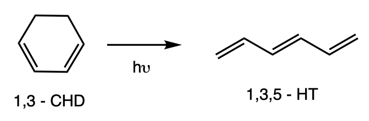
(a) Ring-opening of 1,3-cyclohexadiene (CHD) yields linear HT molecules.

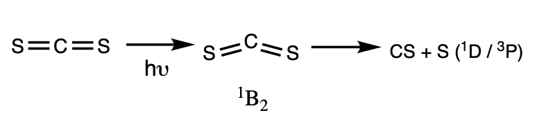
(b) Dissociation of CS2 yields singlet or triplet sulphur atoms.

Figure 1: Schematic of the two photochemical processes probed in the experiments for which data is inverted in this paper, via a basis of trajectory basis functions (TBFs).

3.1 Trajectory basis functions

3.1.1 1,3-cyclohexadiene ring-opening

The ring-opening reaction of 1,3-cyclohexadiene (CHD) to 1,3,5-hexatriene (HT), shown schematically in Figure 1(a), is a prototypical Woodward-Hoffman photoinduced electrocyclic reaction.⁵⁹ It has been the target for a large number of pioneering time-resolved experiments that include UXS, UED, and time-resolved spectroscopies.^{41, 42, 60, 61, 62, 59, 63, 23, 25, 64, 65, 66, 67} Upon absorption of a $267$ nm photon the molecule undergoes a $\pi\rightarrow\pi^{*}$ transition to the steeply sloped 1B electronic state, glancing the conical intersection with the 2A electronic state while staying on the adiabatic potential energy surface. Passage through the conical intersection to the electronic ground state returns the molecule to the original ring-closed CHD or breaks a C-C bond to yield the ring-open HT. A distribution of various cis$\left(Z\right)$/trans$\left(E\right)$ HT isomers are observed given the high internal energy of the system.

Semiclassical trajectories, TBFs, for the dynamics are calculated using the ab initio Ehrenfest (AIMCE) method.^{41, 42} The electronic structure calculations use the ab initio package MOLPRO,⁶⁸ which supplies the forces and the nonadiabatic couplings at 3SA-CAS(6,4)-SCF/cc-pVDZ level of theory for the ground and excited states. A set of 100 TBFs, propagated for 200 fs, with initial conditions sampled from a Wigner distribution in the Franck–Condon region of equilibrium ground state CHD provide the basis for the trajectory-fitting procedure.

3.1.2 CS2 photodissociation

The photodissociation of CS2, shown schematically in Figure 1(b), has been the subject of numerous time-resolved experiments.^{43, 69, 70, 71, 72, 73, 74, 75, 76, 77, 78, 79, 11} Upon excitation to the ${}^{1}B_{2}$ (${}^{1}\Sigma_{u}^{+}$) state rapid bending and stretching vibrational motion is observed. More complex excited state dynamics ensues, exhibiting a striking competition between internal conversion (nonadiabatic couplings) and intersystem crossing (spin-orbit coupling), resulting in two dissociation channels that yield either S(${}^{1}D$) or S(${}^{3}P$) sulphur atoms, with the triplet product dominant.

Semiclassical trajectories (TBFs) to be used in the forward optimisation are calculated using the SHARC surface-hopping package.^{80, 81} The trajectories start on the optically bright ${}^{1}\Sigma_{u}^{+}$ state with a total energy corresponding excitation by a 200 nm pulse and initial coordinates sampled from the ground state Wigner distribution. The forces and nonadiabatic couplings are calculated using SA8-CASSCF(10,8)/SVP electronic structure theory using MOLPRO⁶⁸ and 197 trajectories are propagated for $1$ ps. Further information can be found in SI Section LABEL:sec:ued_treatment.

3.2 Scattering observables

The forward mapping required to compare the model to the UXS and UED data is summarised below. Although scattering signals can be calculated from first principles for gas-phase molecules^{82, 83, 84, 85, 86, 87, 88, 89, 90} and recent x-ray scattering measurements have demonstrated that given sufficient accuracy different electronic states can be resolved,^{91, 92, 10, 93} the experimental data considered in this paper can be modelled using the significantly simpler independent atom model (IAM), which approximates the scattering as a summation over the coherent scattering from isolated atoms.

The instantaneous energy-integrated total scattering cross section into the solid angle $d\Omega$ is then,^{54, 94, 95}

$$\frac{d\sigma}{d\Omega}=\left(\frac{d\sigma}{d\Omega}\right)_{x}I_{\mathrm{mod}}(\mathbf{q}),$$ (10)

where $\mathbf{q}=\mathbf{k}_{0}-\mathbf{k}_{1}$ is the scattering vector expressed in terms of the wave vectors of the incoming and outgoing photon or electron. For x-ray scattering, the prefactor $(d\sigma/d\Omega)_{x}$ is the differential Thomson scattering cross section $(d\sigma/d\Omega)_{\mathrm{Th}}$, here made to include the $|\mathbf{e}_{0}\cdot\mathbf{e}_{1}^{*}|$ polarisation factor, while for electron scattering it is the Rutherford cross section $(d\sigma/d\Omega)_{\mathrm{Rh}}$ which here includes the scaling factor $s^{-4}$.^{96, 97} Note that the expression above does not account for the duration of the x-ray pulse, which is accounted for via the temporal convolution discussed in Section 3.3.

Using the diagonal BAT approximation and assuming time-independent expansion coefficients $\mathinner{\!\left\lVert\mathbf{w}\right\rVert}=1$, the scattering intensity $I(\mathbf{q})$ can be calculated as,

$$I_{\mathrm{mod}}\left(\mathbf{q},t,\mathbf{w}\right)=\sum_{n=1}^{N_{\mathrm{TBF}}}w_{n}I_{n}\left(\mathbf{q},\mathbf{R}_{n}(t)\right).$$ (11)

More general expressions that account for the full wavefunction in eq 6, including the non-local nature of the individual TBF nuclear wavepackets, have been derived previously.⁵⁴ Continuing with the current simplified form, sufficient for our present needs, yields the scattering intensity as,

$$I_{n}(\mathbf{q},\mathbf{R}_{n}(t))=|f(\mathbf{q},\mathbf{R}_{n}(t))|^{2}+S_{\mathrm{inel}}(q),$$ (12)

where $S_{\mathrm{inel}}(q)$ is the inelastic scattering, which is independent of molecular geometry and given by an incoherent summation over the atomic contributions,

$$S_{\mathrm{inel}}(q)=\sum_{A=1}^{N_{\mathrm{at}}}S_{A}(q),$$ (13)

with $N_{\mathrm{at}}$ the number of atoms. The corresponding elastic contribution is given by the form factor $f(\mathbf{q},\mathbf{R}_{n}(t))$,

$$f(\mathbf{q},\mathbf{R}_{n}(t))=\sum_{A=1}^{N_{\mathrm{at}}}f_{A}(q)e^{\imath\mathbf{q}\mathbf{R}_{nA}(t)},$$ (14)

where $f_{A}(q)$ are the atomic form factors and $\mathbf{R}_{nA}(t)$ the position vector for atom $A$ in trajectory $n$. Both $f_{A}(q)$ and $S_{A}(q)$ are tabulated.⁹⁸ The form factors for electron scattering are $f^{\mathrm{e}}=Z_{A}-f^{\mathrm{x}}$, where $Z_{A}$ is the atomic number and $f_{A}^{\mathrm{x}}$ the x-ray scattering form factor.^{96, 97} For high energy electron scattering, notably MeV-UED, it is sometimes necessary to use form factors with relativistic corrections.^{99, 100}

When the target is a gas of anisotropic molecules, rotational averaging of eq 14 results in,¹⁰¹

$$I\left(q,\mathbf{R}_{n}(t)\right)=\sum_{A,B}^{N_{\mathrm{at}}}f_{A}\left(q\right)f_{B}\left(q\right)\frac{\sin{\left(qR_{nAB}(t)\right)}}{qR_{nAB}(t)}\\ \;\;\;\;+S_{\mathrm{inel}}\left(q\right),$$ (15)

with the distance $R_{nAB}(t)=|\mathbf{R}_{nA}(t)-\mathbf{R}_{nB}(t)|$ between atoms $A$ and $B$ in trajectory $n$.

3.3 Apparatus mapping

In this section we discuss the apparatus mapping $S_{j}$ in eq 2 that is required to match the forward mapped signal $X^{j}_{\mathrm{mod}}(t)$ from eq 9 to the experimentally observed signal.

3.3.1 Temporal alignment and convolution

In the scattering experiments, the time-zero is roughly calibrated by the instrument, with the exact time-zero inferred from the observed data. The absence of independent validation means that one must check the alignment of the temporal axes in the experiment and the model. We define the relationship between the experimental and model time axes as $t^{\prime}=t+t_{0}$, where $t^{\prime}$ is the experiment, $t$ the model, and $t_{0}$ the time shift. The temporal alignment $t_{0}$ is one of the global parameters optimised.

A Gaussian convolution in the temporal domain is included as,

$$I_{\mathrm{mod}}^{\mathrm{conv}}(q,t)=\int_{-\infty}^{\infty}I_{\mathrm{mod}}(q,t^{\prime\prime})\;G(t-t^{\prime\prime})\;dt^{\prime\prime},$$ (16)

where $G(t)=b_{c}\exp{(-a_{c}t^{2})}$ mimics the instrument response function, with the normalisation constant given as $b_{c}=\sqrt{4\ln 2/(\tau_{c}^{2}\pi)}$ and $\tau_{c}$ the full-width half-maximum (FWHM). The convolution mainly equates to the cross-correlation of the pump and the probe, effectively compensating for the $\delta(t)$-pulse excitation approximation used to generate the TBFs. In practice, the instrument response function also accounts for other limits on the temporal resolution, such as temporal jitter.

Finally, we note that the experimental resolution with respect to the momentum transfer $q$ is such that no convolution of the model is required. The amount of structural information in the signal is limited by the $q$-range, $q\in[q_{\mathrm{min}},q_{\mathrm{max}}]$, measured in the experiment.^{95, 42}

3.3.2 Percent difference signal

The experimental signal is considered in the percent difference form to minimise systematic multiplicative errors,

$$\%\Delta I_{\mathrm{exp}}\left(q,t^{\prime}\right)=100\frac{I_{\mathrm{on}}\left(q,t^{\prime}\right)-I_{\mathrm{off}}\left(q,t^{\prime}_{j}\ll t_{0}\right)}{I_{\mathrm{off}}\left(q,t^{\prime}_{j}\ll t_{0}\right)},$$ (17)

where $I_{\mathrm{on}}\left(q,t\right)$ is the optically pumped ’laser-on’ signal and $I_{\mathrm{off}}\left(q,t^{\prime}_{j}\leq t_{0}\right)$ is the static ’laser-off’ reference signal measured at delay times $t^{\prime}\ll t_{0}$. The theoretical equivalent is calculated from the model wavefunction $\ket{\Psi_{\mathrm{mod}}\left(t\right)}$ and defined as,

$$\%\Delta I_{\mathrm{mod}}^{\mathrm{conv}}\left(q,t\right)=100\gamma\frac{I_{\mathrm{mod}}^{\mathrm{conv}}\left(q,t\right)-I_{\mathrm{off}}^{\mathrm{th}}\left(q\right)}{I_{\mathrm{off}}^{\mathrm{th}}\left(q\right)},$$ (18)

where the excitation fraction $\gamma$ scales the intensity according to the implicit degree of excitation. The theoretical ’laser-off’ signal $I_{\mathrm{off}}^{\mathrm{th}}\left(q\right)$ is calculated from a suitable reference geometry, or more accurately using a Wigner distribution of the system in its ground state at the equilibrium geometry. In some cases, it may be necessary to modify the definition in eq 18 to scale the signal by the ratio of the integrated intensity of the ’laser-on’ and ’laser-off’ signal, or replace the uniform excitation fraction $\gamma$ with a $q$ dependent excitation fraction $\gamma\left(q\right)$. Such modifications are discussed in the SI.

3.4 Target function and confidence matrix

The experimental percentage difference signal $\%\Delta I_{\mathrm{exp}}\left(q,t\right)$ and the signal predicted from the model $\%\Delta I_{\mathrm{mod}}\left(q,t,w\right)$ give the target function introduced in eq 3 the following specific form,

$$F(\mathbf{w},\mathbf{c})=\sum_{i,j}\left|\%\Delta I_{\mathrm{exp}}(q_{i},t_{j}^{\prime})\right.\\ \;\;\;\;\;\;\;\;\;\;\;\;\left.-\%\Delta I_{\mathrm{mod}}(q_{i},t_{j},\mathbf{w})\right|^{2}p_{\mathrm{conf}}(q_{i},t_{j}^{\prime}),$$ (19)

where $\mathbf{w}=(w_{1},w_{2},\ldots w_{N_{\mathrm{TBF}}})$ are the normalised trajectory weights $\|\mathbf{w}\|=1$, and $\mathbf{c}$ consists of additional global parameters to be optimised, such as e.g. the excitation fraction $\gamma$ and the time-shift $t_{0}$. In principle, more complicated global parameters designed to off-set shortcomings in the quality of the TBFs could be included, such as time-warping to offset inaccuracies in the kinetic energy. The double sum runs over all experimental data points, identified by $q_{i}$ momentum transfer and the temporal coordinates $t_{j}^{\prime}=t_{j}+t_{0}$.

To avoid overfitting of inherently noisy experimental data, the target function includes a confidence matrix. The matrix $p_{\mathrm{conf}}(q_{i},t_{j}^{\prime})$ weights data points, identified by their value of the momentum transfer $q_{i}$ and time bin $t_{j}^{\prime}$, according to the experimental confidence in the accuracy of that data point. For instance, data points subject to poor statistics or systematic errors are given smaller weight while points that are known or expected to be accurate are weighted accordingly. The exact form of $p_{\mathrm{conf}}(q_{i},t_{j}^{\prime})$ depends on the data set, as discussed in the SI.

If needed, one can define a confidence threshold $p_{\mathrm{conf}}^{\mathrm{min}}$, such that all points $p_{\mathrm{conf}}\left(q_{i},t_{j}^{\prime}\right)\leq p_{\mathrm{conf}}^{\mathrm{min}}$ are zero, thus excluding them from the optimisation. The advantage of excluding poor quality points from the optimisation must be balanced against the reduced size of the experimental data set.

3.5 Global optimisation

In the ideal scenario, the experimental signal has sufficient quality (high temporal resolution, large $q$-range, and excellent signal-to-noise) that simultaneous optimisation of all model parameters is possible. Since the number of global parameters is small, the most straightforward approach is to optimise the trajectory weights $\mathbf{w}$ for fixed global parameters $\mathbf{c}$, and to determine from a scan of reasonable values of $\mathbf{c}$ the best overall solution.

For each particular $\mathbf{c}$, a pool of $N_{\mathrm{init}}$ initial weights $\{\mathbf{w}\}_{\mathrm{init}}$ are Monte Carlo sampled with the values of the individual weights in each initial set $w_{i}\in[0,1]$. The target function given in eq 19 is then minimised utilising a non-linear trust-region reflective least-squares algorithm for each initial set. Among the optimisations that converge to a local minimum, within the tolerance constraints, the best minimum is considered a candidate for the global minimum. The number of initial conditions $N_{\mathrm{init}}$ generated in the weight space is increased until apparent convergence is achieved. The convergence of the optimisation with respect to $N_{\mathrm{init}}$ is discussed in SI, Section LABEL:sec:condition_convergence. In challenging cases, an iterative approach using more targeted sampling can be used, which is discussed in the SI.

3.6 Two-step optimisation

When the experimental data is of lower quality, more stable solutions are found via a two-step optimisation procedure. The first step ensures that global parameters, such as $t_{0}$ and $\tau_{c}$, are determined as accurately as possible before, in the second step, optimisation of the trajectory weights is attempted.

3.6.1 Step 1: Global parameters

First, we identify the strongest features in the data by inspection of the confidence matrix $p_{\mathrm{conf}}(q_{i},t_{j}^{\prime})$. This allows us to minimise the negative effects of noise on the optimisation. Selecting the strongest feature, we define the net integrated percentage difference signal as,

$$\%\Delta I^{\mathrm{int}}\left(t\right)=\int_{q^{\mathrm{conf}}_{\mathrm{min}}}^{q^{\mathrm{conf}}_{\mathrm{max}}}\%\Delta I\left(q,t\right)dq,$$ (20)

where $q^{\mathrm{conf}}_{\mathrm{min}}$ and $q^{\mathrm{conf}}_{\mathrm{max}}$ are the bounds on the section of highest confidence. The global parameters $\mathbf{c}$ are then optimised against this integrated signal, $\%\Delta I^{\mathrm{int}}_{\mathrm{exp}}\left(t\right)$. Since this step must be performed independently from the optimisation of the trajectory weights $\mathbf{w}$, we assume that the $t\approx t_{0}$ wavefunction can be approximated by an equally weighted sum of TBFs. This is reasonable given the limited dispersion and dephasing in the wavepacket at early times.

The $t_{0}$ is inherently linked to $\tau_{c}$ and $\gamma$ since the pulse width $\tau_{c}$ affects the onset of the signal and $\gamma$ scales the strength of the signal. Therefore, for different combinations of $t_{0}$ and $\tau_{c}$, the sum of square error between the experimental and model integrated difference signal in eq 20 is minimised with the $\gamma$ excitation fraction as the free parameter.

3.6.2 Step 2: TBF weights

The second step in the optimisation takes the best values of $\left(t_{0},\tau_{c},\gamma\right)$ from the previous step with the goal of identifying the optimal trajectory weights $\mathbf{w}$. Since the $\gamma$ in step one is determined on the assumption of equally weighted TBFs, the parameter $\gamma$ is reoptimised alongside the weights $\mathbf{w}$ in this second step. If the final value of $\gamma$ diverges significantly from its initial value, this may indicate that the parameters determined in the first step are not optimal. In order to ensure self-consistency, it is advisable to repeat the second step optimisation for several different sets of global parameter values $\left(t_{0},\tau_{c},\gamma\right)$ which correspond to good fits in the first step. The procedure is complete once the best sets of these values from step one and two agree, and when the target function $F(\mathbf{w},\mathbf{c})$ has converged.

3.7 Metrics of fit quality

In addition to the target function $F(\mathbf{w},\mathbf{c})$, it is useful to have other measures of the quality of the fit. The improvement in overall agreement between the unweighted and weighted model function can be quantified by the relative absolute error (RAE),

$$\begin{split}&\mathrm{RAE}=\\ &\frac{1}{N_{t}}\sum_{t}\frac{|\frac{1}{N_{q}}\sum_{q}\%\Delta I_{\mathrm{mod}}(q,t)-\%\Delta I_{\mathrm{exp}}(q,t)|}{|\frac{1}{N_{q}}\sum_{q}\%\Delta I_{\mathrm{th}}(q,t)-\%\Delta I_{\mathrm{exp}}(q,t)|},\end{split}$$ (21)

where $N_{t}$ is the number of time steps, $N_{q}$ the number of points in $q$, and $\%\Delta I_{\mathrm{th}}(q,t)$ the theoretical signal calculated from the theoretical wavefunction not subjected to any bias or optimisation. The RAE measure, as defined above, is independent of the size of the $N_{t}\crossproduct N_{q}$ grid. Another helpful metric is the root mean squared error (RMSE) defined as,

$$\mathrm{RMSE}=\sum_{q,t}\frac{|\%\Delta I_{\mathrm{mod}}(q,t)-\%\Delta I_{\mathrm{exp}}(q,t)|}{N_{q}N_{t}}.$$ (22)

Particular solutions can also be characterised using the variance of the $N_{\mathrm{TBF}}$ weights from a single optimisation, i.e. the spread of weights resulting from one of the $N_{\mathrm{init}}$ initial conditions (typically the initial condition that yields the best solution for a specific set of global parameters), defined as,

$$v_{w}^{2}=\sum_{n=1}^{N_{\mathrm{TBF}}}|w_{n}-\left<\mathbf{w}\right>|^{2},$$ (23)

where $\left<\mathbf{w}\right>$ is the mean of the weights. In addition, to compare different solutions we define the distance $D_{b}$ from the overall best set of optimised weights,

$$D_{b}^{2}=|\mathbf{w}_{b}-\mathbf{w}_{\mathrm{best}}|^{2},$$ (24)

which describes the distance for a particular solution $b$ from the best set of optimised weights.

4 Experimental data

4.1 Ultrafast x-ray scattering

The ultrafast x-ray scattering (UXS) data for the ring-opening reaction of CHD shown in Figure 2 is taken from ref 42 (further details in the SI, Section LABEL:sec:uxs_treatment). The confidence matrix $p_{\mathrm{conf}}$ in eq 3 in this case is based on the number of photon hits per frame (SI, eq LABEL:eqn:conf_mat_xray). Due to a long interaction region in these experiments, we include a $q$-dependent excitation fraction $\gamma\left(q\right)$ which is indirectly optimised by allowing it to be uniformly scaled by a factor $x$ such that it yields the scaled excitation fraction $\gamma_{x}\left(q\right)$ (for more details see the SI). Accounting for the convolution of the signal as in eq 16 and the subsequent temporal binning into bins of size $\Delta t=25$ fs, the total length of the signal used becomes 275 fs.

The quality of the experimental data allows a one-step global optimisation in which we scan over a range of $t_{0}$ values and $x$ scaling factors, where $t_{0}\in\left[-38,-14\right]$ and $x\in\left[0.7,1.3\right]$. The duration of the pump and probe pulse were measured from experiment as 60 fs and 30 fs respectively, which fixes the value of $\tau_{c}$.

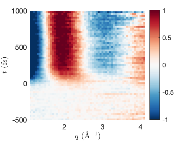
Figure 2: A subsection of the experimental UXS signal $\%\Delta I_{\mathrm{exp}}(q,t)$ for CHD from ref 42. The experimental signal has been shifted in time so that it is centered at $t=0$, instead of the $t^{\prime}=-110$ fs along the original raw experimental time axis.

4.2 Ultrafast electron diffraction

The ultrafast electron diffraction (UED) data for the photodissociation of CS2 is taken from ref 43 (further details in the SI, Section LABEL:sec:ued_treatment). The data does not support the real-space pair distribution function (PDF) analysis obtained by a sine-transform of the modified scattering signal $\Delta sM$ that is common in UED (see SI, Section LABEL:sec:pdf_limitations). Instead, the signal is evaluated in the percent difference form as per eq 17.

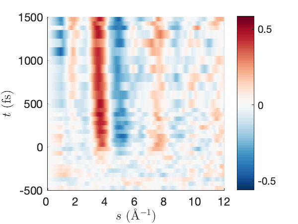
Figure 3: A subsection of the UED signal $\%\Delta I_{\mathrm{exp}}(s,t)$ for CS2 from ref 43. The signal is initially centred on $t^{\prime}=-120$ fs.

The experimental signal $\%\Delta I_{\mathrm{exp}}(s,t)$ in Figure 3 displays a strong enhancement band (red) next to a strong depletion band (blue) in the range $3.5<s<6.0$ Å^-1. Also note less intense enhancement/depletion features for $s<2$ Å^-1 which appear at later times and which correlate with the onset of strong dissociation.

Given the noise and limited temporal resolution in the data, we carry out a two-step optimisation. In the first step, we fit $t_{0}$ using eq 20 with bounds $[s_{\mathrm{min}},s_{\mathrm{max}}]=[2.8,4.2]$ Å^-1. This procedure is repeated in the range $t_{0}\in\left[-16,83\right]$ fs and $\tau_{c}\in\left[150,250\right]$ fs. The best global parameters are then used in the determination of the weights $\mathbf{w}$. Initial conditions for $\mathbf{w}$ are generated both using unbiased Monte Carlo sampling and using the biased iterative sampling procedure described in SI, Section. LABEL:sec:weights. In either case, the confidence matrix $p_{\mathrm{conf}}$ is based on estimated experimental standard deviations (see SI, eq LABEL:eq:conf_mat_ued).

5 Results and Discussion

5.1 CHD ring-opening (UXS)

For the CHD reaction, the data is of sufficient quality that a global one-step optimisation is feasible. Optimisation yields the best fit parameters $\left[t_{0},x\right]=[-38\;\mathrm{fs},1.3]$, with a RAE of $0.775$. Recall, the scaling factor $x$ is optimised as to uniformly scale the $q$ dependent excitation fraction such that, $\gamma_{x}\left(q\right)=\gamma\left(q\right)x$. The values of $\gamma\left(q\right)$ and the resulting optimised $\gamma_{x}\left(q\right)$ over the available $q$ range, can be seen in SI Figure LABEL:fig:chd_xfrac. The convergence with respect to $x$ and the $t_{0}$ shift in Figure 4 shows that more negative $t_{0}$ shifts and larger $x$ result in lower values of the target function $F\left(\mathbf{w},\mathbf{c}\right)$ and better RAE’s (with the trend more pronounced for higher $x$). Generally, $F\left(\mathbf{w},\mathbf{c}\right)$ is more sensitive to $x$ than $t_{0}$.

The change in the fraction of ring-open trajectories is small as $t_{0}$ changes, which is unsurprising given that the majority of the ring-opening occurs in a concerted fashion within the first 140 fs.⁵⁹ Current literature values are found in the range 40-60%.⁵⁹ We note that higher values of $x$ redistribute some of the ring-open weights to ring-closed weights. Since one does not physically expect the fraction of open to closed trajectories to change as a function of the excitation fraction, this is an artefact which stems from the fact that the percent difference signal is stronger for ring-open molecules than ring-closed, due to the reference equilibrium CHD structure being ring-closed. In principle, this could be addressed by a different choice of reference structure.

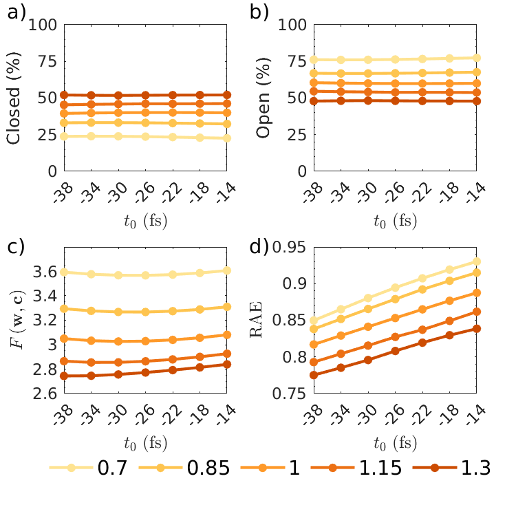
Figure 4: Convergence in the CHD optimisation, showing the a) ring-closed fraction, b) ring-open fraction, c) the target function and d) the relative absolute error (RAE) as a function of $t_{0}$. Each colour represents a different value of the scaling factor $x$, ranging from 0.7 to 1.3.

The eight dominant trajectories in the final solution are summarised in Table 1. These account for almost all the weights. The trajectories can be visualised in terms of their characteristic C1-C6 bond distance as shown in Figure 5. Three main families of trajectories are observed: direct ring-opening, a slower indirect ring-opening which undergoes several C1-C6 stretches before breaking the bond, and finally ring-closed paths with initially strong oscillations in the C1-C6 bond which are damped out as the energy disperses across all motions. In total, the ring-opening and closed trajectories have a weight of 52 % and 48 % respectively.

The ground state HT has several cis-/trans- $\left(Z\right)/\left(E\right)$ isomers. Out of the 48% HT product, we predominately observe the presence of cEc-HT (8.7%) and cZc-HT (34.5%) isomers. Due to the length of the 275 fs temporal window used in the fit it is no surprise we can not clearly detect the tZt-HT isomer. However, we note that we observe a small fraction (3.4%) with a configuration between cZt and tZt. With data available over a longer temporal range, one could better refine the ground state dynamics and eventually observe as the system settles into a thermal equilibrium between different HT isomers.

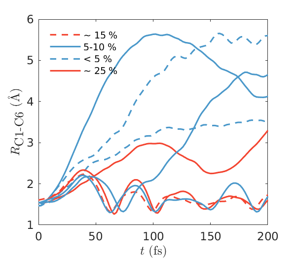
Figure 5: C1-C6 distances for the eight CHD trajectories with a weight greater than 1%. There are three distinct classes of trajectories: ring-closed, direct ring-opening and indirect (delayed) ring-opening.

Weight (%)	Type
28.4	open (indirect)
27.3	closed
15.1	closed
9.70	closed
8.70	open
6.05	open (indirect)
3.38	open
1.35	open

Table 1: Weights of the dominant trajectories from the forward optimisation for CHD, along with their type.

In Figure 6, one can see there is little variation from the best set of weights if one examines solutions with more negative $t_{0}$ shifts or larger $x$. The cluster of very good optimisations are all found within a small radius of $D_{b}^{2}$ from the optimal solution, and have RAE’s in the range 0.77-0.82 with only a slight re-weighting of similar trajectories. The solutions are further removed when when $x=\left[0.7,0.85\right]$, which is a consequence of the optimisation redistributing weight between ring-closed trajectories and selecting a different set of ring-opening trajectories. In addition, we note that the better optimisations (as measured by their RAE) tend to exhibit a larger variance in their set of weights, this can be seen in SI Figure LABEL:fig:chd_var_weights.

Figure 6: Square distances $D_{b}^{2}$ (eq 24) of the weights from a series of different optimisations relative the best weights with $\left[t_{0},x\right]=\left[-38,1.3\right]$, plotted against the relative absolute error (RAE). Each shade represents a different $t_{0}$ ranging from -38 to -14 fs (the darker the shade, the earlier the $t_{0}$ shift).

5.2 CS2 photodissociation (UED)

We now turn to the more difficult case of CS2, where the resolution forces us to employ the two-step optimisation procedure. The first step of optimisation yields the optimal global parameters $\left[t_{0},\tau_{c},\gamma\right]=\left[-83\textrm{~{}fs},230\textrm{~{}fs},3\%\right]$. Figure 7 shows that not only does $t_{0}=-83$ fs and $\tau_{c}=230$ fs result in the lowest value of $F\left(\mathbf{w},\mathbf{c}\right)$, but also that the two complementary error measures RAE and RMSE confirm this. These parameters also yield smoother convergence across all values of $\tau_{c}$ in comparison to other values of $t_{0}=\left[+17,-33\right]$. The resulting final best fit in step one is shown in Figure 8. The model tracks the experimental data closely, especially in the important region around $t=0$, while at other times the rather scattered experimental data is contained with one standard deviation of the model, with the standard deviation calculated on the whole ensemble of trajectories relative the equally-weighted ’average’ model. Also note the significant noise floor in the experimental data evident for $t\ll 0$. This emphasises the importance of a robust method for fitting, inverting, and interpreting the experimental data.

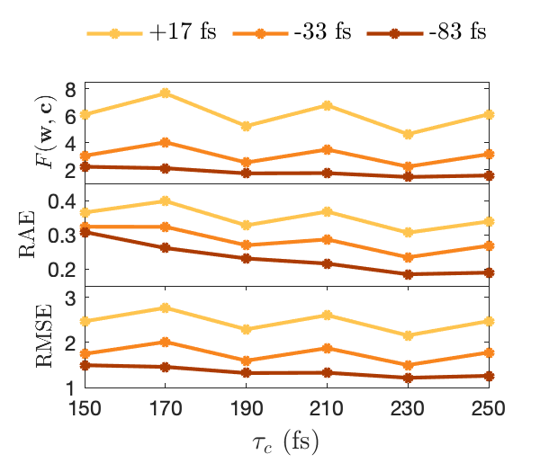
Figure 7: Convergence of the step one optimisation with respect to $t_{0}$ and $\tau_{c}$. The panels show the convergence of the target function $F(\mathbf{w},\mathbf{c})$ (top), the RAE (middle), and RMSE (bottom).

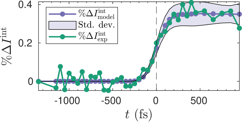
Figure 8: Final result for the step one optimisation against the integrated intensity $\%\Delta I_{\mathrm{model}}^{\mathrm{int}}$ (eq 20 with equal weights). The model is convoluted with a Gaussian with $\tau_{c}=230$ fs (FWHM) and the optimised value of excitation fraction is $\gamma=3\%$. The shaded area indicates the standard deviation of the ensemble of trajectories from the model calculated assuming equal weights.

For the second step of the optimisation, we take the global parameters determined in step one as the starting point for the unconstrained determination of the TBF weights $\mathbf{w}$. We also repeat the procedure for three different values of $t_{0}$ to check that the optimisations are consistent. During optimisation, the pre-determined value of the global parameter $\gamma$ is allowed to readjust. The value should change little but if it does change significantly this may indicate that the values from step one are suboptimal.

The weighting of the diffraction signal with the confidence matrix, $p_{\mathrm{conf}}\left(s_{i},t_{j}^{\prime}\right)$, is crucial to achieve a sensible fit, with significantly poorer results obtained without it. To investigate this effect, the optimisation was repeated for several values of the confidence matrix cut-off threshold, $p_{\mathrm{conf}}^{\mathrm{min}}\in[0,0.45,0.50,0.55,0.60,0.65]$. As seen in SI Figure LABEL:fig:cs2_confmats, increasing the threshold corresponds to hard filtering of the data and lower thresholds correspond to including more data. For example, $p_{\mathrm{conf}}^{\mathrm{min}}=0$ includes all data, while $p_{\mathrm{conf}}^{\mathrm{min}}=0.65$ only includes the main feature in Figure 3. Examining the RAE in Figure 9d, it is evident that at all values of $t_{0}$, high $p_{\mathrm{conf}}^{\mathrm{min}}$ is detrimental to the optimisation and $p_{\mathrm{conf}}^{\mathrm{min}}=0$ yields the best results. This suggests that including all data is beneficial as long as the data is given appropriate confidence weights. This is further confirmed by examining the physical observables resulting from the inversion, as discussed next.

Figures 9a-c show the convergence of three physical observables as a function of the convergence threshold $p_{\mathrm{conf}}^{\mathrm{min}}$ for $t_{0}=[17,-33,-83]$ fs. The observables are not explicitly part of the fit, but are indirectly a function of the optimised weights. The branching ratio between singlet and triplet dissociation product varies significantly over the range of times and confidence thresholds, and convergence to the spectroscopy-derived literature value ($\approx 3$) is only obtained for $t_{0}=83$ fs and then only at low values of confidence threshold $p_{\mathrm{conf}}^{\mathrm{min}}\rightarrow 0$. In contrast, the convergence of the fraction of bound trajectories at 1 ps is more uniform across the different $t_{0}$ values. Values in the range of 20-30%, congruent with spectroscopic results, are observed for the lower confidence thresholds. A similar trend can be observed for the excitation fraction $\gamma$, which is comparatively stable across all values of $t_{0}$ and $p_{\mathrm{conf}}^{\mathrm{min}}$. This indicates that a suitable choice of $\tau_{c}$ was made and is also reflective of the fact that the value of $\gamma$ is most governed by the strongest feature in the experimental data (which is also recorded with the lowest noise).

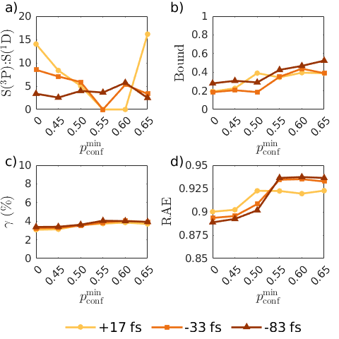
Figure 9: Convergence in CS2 optimisation (step two) as a function of confidence threshold $p_{\mathrm{conf}}^{\mathrm{min}}$ for three values of $t_{0}$, showing a) branching ratio, b) bound fraction at 1 ps, c) excitation fraction $\gamma$, and d) relative absolute error (RAE).

Weight (%)	Type
44.7	Triplet
17.8	Bound
10.4	Singlet
10.2	Bound
7.42	Triplet
4.42	Singlet
3.39	Triplet
1.67	Singlet

Table 2: Weights of the dominant trajectories in the best forward optimisation for CS2.

Overall, the best optimisation yields the final values $\left[t_{0},\tau_{c},\gamma,p_{\mathrm{conf}}^{\mathrm{min}}\right]=\left[-83\textrm{~{}fs},230\textrm{~{}fs},3.4\%,0\right]$, with the convergence of $F\left(\mathbf{w},\mathbf{c}\right)$ shown in Figure LABEL:fig:cs2_tfunc in the SI for reference. The initial guess of $\gamma=3.0\%$ from step one is reoptimised to $3.4\%$ in the second step, with the comparatively small change suggestive of a stable solution. Examination of the optimised weights show that eight dominant trajectories account for $99.9$% of the total weight. Two of these are bound trajectories that make up a total of $28$%, three correspond to singlet dissociation, and two to triplet dissociation, which gives a branching ratio of singlet to triplet of 1:3.38. A summary of the eight trajectories is given in Table 2. The contributions from each of dissociative and bound classes of trajectories to the model signal $\%\Delta I_{\mathrm{mod}}\left(s,t\right)$ can be seen in SI Figure LABEL:fig:cs2_signal_decomp. From this we attribute the onset of the peak below 2 Å^-1 in the experimental signal $\%\Delta I_{\mathrm{exp}}\left(s,t\right)$ to dissociation.

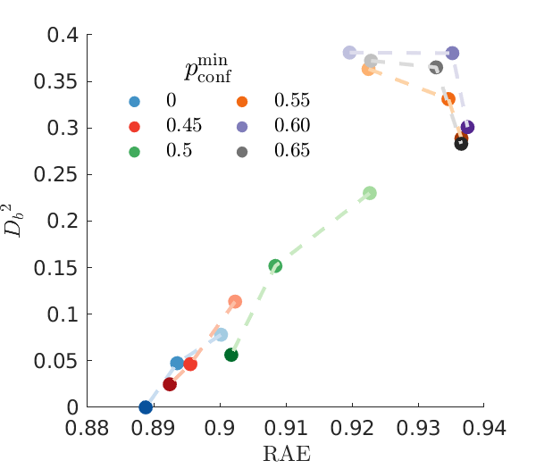
Figure 10: Squared distances $D_{b}^{2}$ (eq 24) of the final TBF weights for CS2, examining a series of different optimisations relative the best solution with $\left(t_{0},\tau_{c},\gamma,p_{\mathrm{conf}}^{\mathrm{min}}\right)=\left(-83,230,3.4,0\right)$. The results are plotted with the relative absolute error (RAE) on the $x$-axis. For each value of $p_{\mathrm{conf}}^{\mathrm{min}}$, the varying opacity represents a different $t_{0}$ shift, ranging from -83, -33 to +17 fs from dark to light respectively.

In Figure 10 we see that the set of very good solutions, as judged by their RAE value, cluster around the best solution as measured by the distance $D_{b}$ (eq 24). Broadly, this indicates that the optimisation procedure succeeds in locating robust global optima. The clustering trend is especially evident when $p_{\mathrm{conf}}^{\mathrm{min}}\leq 0.5$ and $t_{0}=\left[-83,-33\right]$. As the value of $p_{\mathrm{conf}}^{\mathrm{min}}$ increases and $t_{0}$ is shifted towards earlier times, the distances increase. These deviations at high values of $p_{\mathrm{conf}}^{\mathrm{min}}$ are explained by the fact that the bound population at 1 ps is over-estimated due to the omission of a distinct feature just below 2 Å^-1 with a delay in the onset of the characteristic of dissociation (see Figure 3). As with CHD, we see that the better optimisations (as measured by their RAE) also exhibit a larger variance in their set of weights, this can be seen in SI Figure LABEL:fig:cs2_var_weights.

It is worth noting that for the best $t_{0}$ and for each confidence threshold, the optimisation converges to some combination of the same subset of 16 trajectories. While only 8 of these are significant in the best optimisation where $(p_{\mathrm{conf}}^{\mathrm{min}})=0$, generally the weights of these trajectories show little variation as a function of the confidence threshold. Some are re-weighted significantly, for example the dominant triplet trajectory with a weight of nearly 45% only appears in the set of trajectories once the confidence threshold is lowered and more data included. The same is true of a singlet trajectory which sees its weight increase $0\%\rightarrow 4.5$% as the confidence threshold is decreased. The opposite effect is seen for a triplet trajectory and a bound trajectory. As more data is included, these trajectories see their weight decrease $20\%\rightarrow 7.5$% and $32\%\rightarrow 18$%, respectively. Thus the contribution of some trajectories can be over-estimated and the contribution of others under-estimated when the optimisation is based on high confidence thresholds, i.e. smaller data sets.

A closer examination of the distribution of trajectory weights as a function of $t_{0}$ shows that the relative distribution between singlet and triplet trajectories is sensitive to $t_{0}$. This is not surprising given that singlet and triplet dissociation is separated temporally, with the singlet dissociation appearing earlier. Shifts in the temporal alignment of experiment and model thus forces the optimisation to try to compensate by changing the relative composition of the singlet vs triplet dissociation.

Finally, using the iterative weight sampling procedure outlined in the SI, we can confirm that convergence to the global minimum is achieved for the parameters $[t_{0},\tau_{c},\gamma,p_{\mathrm{conf}}^{\mathrm{min}}]=\left[-83~{}\mathrm{fs},230~{}\mathrm{fs},3.4\%,0\right]$ (for further details, see the SI).

6 Conclusions

In this paper, we have presented a forward optimisation method for the inversion of time-resolved data and evaluated its performance on data from actual experiments. The method matches experimental data to a model molecular wavefunction by optimising the weights of trajectory basis functions (TBFs). The TBFs provide appropriate constraints on molecular systems far from equilibrium and ensure that continuity relations are fulfilled. The method can be applied to any type of experiment for which observables can be calculated from the model wavefunction and to any molecular system for which a basis of trajectories can be generated.

Notably, the TBFs ensure a physically sensible solution even when the inversion is underdetermined by the available data, which is the common situation in ultrafast experiments where the observable often only illuminates one specific aspect of the complex dynamics, or when the data has limited temporal, spatial, or energy resolution (for instance a limited $q$-range in scattering experiments). Importantly, we demonstrate that our approach is robust for noisy data and show that using a confidence matrix for the experimental data is far superior to excluding noisy data from the inversion. For very noisy data, we use a two-step optimisation which first optimises global parameters and then the model wavefunction.

We apply the method to ultrafast scattering data for the molecules CS2 and CHD. Good agreement with the experimental data is found, and the model performs well also on additional quality measures introduced to evaluate the model wavefunction and the stability of the solution. The appraisal of the solution includes comparison to spectroscopic data not included for in the inversion, with the optimised model reproducing key physical properties such as the branching ratio of ring-open to ring-closed product molecules for CHD and the ratio of singlet to triplet dissociation products in CS2.

The procedure allows key dynamic motifs that contribute to the signal to be identified. For CHD, the method disentangles three pathways involved in the ring-opening and for CS2 it identifies a key marker of dissociation in the signal.

Ultrafast experiments tend to include theory and simulations as part of their analysis. The current approach fits naturally into this workflow by allowing the discrepancies between theory and experiment to be identified while providing a robust interpretation of the experimental data. The forward optimisation analysis can be performed at small additional cost and provides a bridge between the theory and the experiment, and introduces a systematic strategy for addressing potential shortcomings in simulations.

Looking ahead, forward optimisation should be applied to other observables and, more importantly, to combined data sets (e.g. photoelectron spectroscopy and scattering data). For scattering experiments specifically, higher quality data will potentially allow for the inversion to account for state-specific scattering,^{83, 87} inelastic effects,^{102, 103} possibly coherent mixed scattering,¹⁰⁴ and, finally, alignment effects.¹⁰⁵ Sophisticated analysis of multidimensional, low-noise data is a prerequisite for unambiguous identification of subtle yet important effects in photochemical dynamics, including interferences or passage through conical intersections, and inversion methods are expected to play an increasingly central role in ultrafast imaging.

KA acknowledges an EPSRC doctoral studentship and a public engagement scholarship from the University of Edinburgh. AK acknowledges funding from the EPSRC (EP/V006819 and EP/V049240) and the Leverhulme Trust (RPG-2020-208). This work was also supported by the Department of Energy, Office of Science, Basic Energy Sciences, under award number DE-SC0020276. Finally, AK acknowledges a Fellowship at the Swedish Collegium for Advanced Studies with financial support from the Erling-Persson Family Foundation and the Knut and Alice Wallenberg Foundation.

Further details are provided in the Supplementary Information.

References

- Tanaka and Dulikravich 1998 Tanaka, M., Dulikravich, G. S., Eds. Inverse problems in engineering mechanics: International Symposium on Inverse Problems in Engineering Mechanics; Elsevier: Amsterdam; New York, 1998
- Razavy 2020 Razavy, M. An Introduction to Inverse Problems in Physics; World Scientific, 2020
- Tanaka et al. 2021 Tanaka, A.; Tomiya, A.; Hashimoto, K. Deep Learning and Physics; Mathematical Physics Studies; Springer Singapore: Singapore, 2021
- Giraud and Thas 2010 Giraud, O.; Thas, K. Hearing shapes of drums: Mathematical and physical aspects of isospectrality. Rev. Mod. Phys. 2010, 82, 2213–2255
- Arridge 1999 Arridge, S. R. Optical tomography in medical imaging. Inverse Probl. 1999, 15, R41–R93
- Bertero and Piana 2006 Bertero, M.; Piana, M. In Complex Systems in Biomedicine; Quarteroni, A., Formaggia, L., Veneziani, A., Eds.; Springer Milan: Milano, 2006; pp 1–33
- Huber and Herzberg 1979 Huber, K. P.; Herzberg, G. Molecular spectra and molecular structure IV. Constants of diatomic molecules., 1st ed.; Van Nostrand Reinhold: New York, 1979
- McMorrow and Als-Nielsen 2011 McMorrow, D.; Als-Nielsen, J. Elements of Modern X-Ray Physics, 2nd ed.; Wiley-Blackwell, 2011
- Hargittai and Hargittai 1988 Hargittai, I.; Hargittai, M. Stereochemical applications of gas-phase electron diffraction: Part A The Electron Diffraction Technique, 1st ed.; VCH: New York, 1988
- Stankus et al. 2019 Stankus, B.; Yong, H.; Zotev, N.; Ruddock, J. M.; Bellshaw, D.; Lane, T. J.; Liang, M.; Boutet, S.; Carbajo, S.; Robinson, J. S.; Du, W.; Goff, N.; Chang, Y.; Koglin, J. E.; Minitti, M. P.; Kirrander, A.; Weber, P. M. Ultrafast X-ray scattering reveals vibrational coherence following Rydberg excitation. Nat. Chem. 2019, 11, 716–721
- Gabalski et al. 2022 Gabalski, I.; Sere, M. A.; Acheson, K.; Allum, F.; Boutet, S.; Dixit, G.; Forbes, R.; Glownia, J. M.; Goff, N.; Hegazy, K.; Howard, A. J.; Liang, M.; Minitti, M. P.; Minns, R. S.; Natan, A.; Peard, N.; Razmus, W. O.; Sension, R. J.; Ware, M. R.; Weber, P. M.; Werby, N.; Wolf, T. J. A.; Kirrander, A.; Bucksbaum, P. Transient vibration and product formation of photoexcited CS2 measured by time-resolved X-ray scattering. J. Chem. Phys. 2022,
- Yong et al. 2021 Yong, H.; Carrascosa, A. M.; Ma, L.; Stankus, B.; Minitti, M. P.; Kirrander, A.; Weber, P. M. Determination of excited state molecular structures from time-resolved gas-phase X-ray scattering. Faraday Discuss. 2021, 228, 104–122
- Zewail 2000 Zewail, A. H. Femtochemistry: Atomic-Scale Dynamics of the Chemical Bond Using Ultrafast Lasers (Nobel Lecture). Angew. Chem. Int. Ed. 2000, 39, 2586–2631
- Stolow et al. 2004 Stolow, A.; Bragg, A. E.; Neumark, D. M. Femtosecond Time-Resolved Photoelectron Spectroscopy. Chem. Rev. 2004, 104, 1719–1758
- Neville et al. 2016 Neville, S. P.; Averbukh, V.; Patchkovskii, S.; Ruberti, M.; Yun, R.; Chergui, M.; Stolow, A.; Schuurman, M. S. Beyond structure: ultrafast X-ray absorption spectroscopy as a probe of non-adiabatic wavepacket dynamics. Faraday Discuss. 2016, –
- Capano et al. 2015 Capano, G.; Milne, C. J.; Chergui, M.; Rothlisberger, U.; Tavernelli, I.; T J Penfold, Probing wavepacket dynamics using ultrafast x-ray spectroscopy. J. Phys. B 2015, 48, 214001
- Centurion 2016 Centurion, M. Ultrafast imaging of isolated molecules with electron diffraction. J. Phys. B: At. Mol. Opt. Phys. 2016, 49, 062002
- Ischenko et al. 2017 Ischenko, A. A.; Weber, P. M.; Miller, R. J. D. Capturing Chemistry in Action with Electrons: Realization of Atomically Resolved Reaction Dynamics. Chem. Rev. 2017, 117, 11066–11124
- Budarz et al. 2016 Budarz, J. M.; Minitti, M. P.; Cofer-Shabica, D. V.; Stankus, B.; Kirrander, A.; Hastings, J. B.; Weber, P. M. Observation of Femtosecond Molecular Dynamics via Pump-probe Gas Phase X-Ray Scattering. J. Phys. B 2016, 49, 034001
- Stankus et al. 2020 Stankus, B.; Yong, H.; Ruddock, J.; Ma, L.; Carrascosa, A. M.; Goff, N.; Boutet, S.; Xu, X.; Zotev, N.; Kirrander, A.; Minitti, M.; Weber, P. M. Advances in Ultrafast Gas-Phase X-ray Scattering. J. Phys. B: At. Mol. Opt. Phys. 2020,
- Rolles 2023 Rolles, D. Time-resolved experiments on gas-phase atoms and molecules with XUV and X-ray free-electron lasers. Adv. Phys. X 2023, 8, 2132182
- Kim et al. 2015 Kim, K. H.; Kim, J.; Oang, K. Y.; Lee, J. H.; Grolimund, D.; Milne, C. J.; Penfold, T. J.; Johnson, S. L.; Galler, A.; Kim, T. W.; Kim, J. G.; Suh, D.; Moon, J.; Kim, J.; Hong, K.; Guérin, L.; Kim, T. K.; Wulff, M.; Bressler, C.; Ihee, H. Identifying the major intermediate species by combining time-resolved X-ray solution scattering and X-ray absorption spectroscopy. Phys. Chem. Chem. Phys. 2015, 17, 23298–23302
- Pemberton et al. 2015 Pemberton, C. C.; Zhang, Y.; Saita, K.; Kirrander, A.; Weber, P. M. From the (1B) Spectroscopic State to the Photochemical Product of the Ultrafast Ring-Opening of 1,3-Cyclohexadiene: A Spectral Observation of the Complete Reaction Path. J. Phys. Chem. A 2015, 119, 8832–8845
- Stankus et al. 2016 Stankus, B.; Budarz, J. M.; Kirrander, A.; Rogers, D.; Robinson, J.; Lane, T. J.; Ratner, D.; Hastings, J.; Minitti, M. P.; Weber, P. M. Femtosecond photodissociation dynamics of 1,4-diiodobenzene by gas-phase X-ray scattering and photoelectron spectroscopy. Faraday Discuss. 2016, 194, 525–536
- Tudorovskaya et al. 2018 Tudorovskaya, M.; Minns, R. S.; Kirrander, A. Effects of probe energy and competing pathways on time-resolved photoelectron spectroscopy: the ring-opening of 1,3-cyclohexadiene. Phys. Chem. Chem. Phys. 2018, 20, 17714–17726
- Yong et al. 2019 Yong, H.; Ruddock, J. M.; Stankus, B.; Ma, L.; Du, W.; Goff, N.; Chang, Y.; Zotev, N.; Bellshaw, D.; Boutet, S.; Carbajo, S.; Koglin, J. E.; Liang, M.; Robinson, J. S.; Kirrander, A.; Minitti, M. P.; Weber, P. M. Scattering off molecules far from equilibrium. J. Chem. Phys. 2019, 151, 084301
- Yong et al. 2021 Yong, H.; Carrascosa, A. M.; Ma, L.; Stankus, B.; Minitti, M. P.; Kirrander, A.; Weber, P. M. Determination of excited state molecular structures from time-resolved gas-phase X-ray scattering. Faraday Disc. 2021, 228, 104–122
- Habershon and Zewail 2006 Habershon, S.; Zewail, A. H. Determining Molecular Structures and Conformations Directly from Electron Diffraction using a Genetic Algorithm. Chem. Phys. Chem. 2006, 7, 353–362
- Hensley et al. 2012 Hensley, C. J.; Yang, J.; Centurion, M. Imaging of Isolated Molecules with Ultrafast Electron Pulses. Phys. Rev. Lett. 2012, 109, 133202
- Yang et al. 2013 Yang, J.; Hensley, C. J.; Centurion, M. Ultrafast 3D imaging of isolated molecules with electron diffraction. 2013; p 884502
- Yang et al. 2014 Yang, J.; Zandi, O.; Zhang, P.; Centurion, M. Imaging of molecules in the gas phase with ultrafast electron diffraction. 2014; pp 100–110
- Yang et al. 2014 Yang, J.; Makhija, V.; Kumarappan, V.; Centurion, M. Reconstruction of three-dimensional molecular structure from diffraction of laser-aligned molecules. Struct. Dyn. 2014, 1, 044101
- Saldin et al. 2011 Saldin, D. K.; Poon, H. C.; Bogan, M. J.; Marchesini, S.; Shapiro, D. A.; Kirian, R. A.; Weierstall, U.; Spence, J. C. H. New Light on Disordered Ensembles: Ab Initio Structure Determination of One Particle from Scattering Fluctuations of Many Copies. Phys. Rev. Lett. 2011, 106, 115501
- Saldin et al. 2010 Saldin, D. K.; Shneerson, V. L.; Starodub, D.; Spence, J. C. H. Reconstruction from a single diffraction pattern of azimuthally projected electron density of molecules aligned parallel to a single axis. Acta Crystallogr. A 2010, 66, 32–37
- Saldin et al. 2011 Saldin, D. K.; Poon, H.-C.; Schwander, P.; Uddin, M.; Schmidt, M. Reconstructing an icosahedral virus from single-particle diffraction experiments. Opt. Express, OE 2011, 19, 17318–17335
- Shneerson et al. 2008 Shneerson, V. L.; Ourmazd, A.; Saldin, D. K. Crystallography without crystals. I. The common-line method for assembling a three-dimensional diffraction volume from single-particle scattering. Acta Crystallogr. A 2008, 64, 303–315
- Fung et al. 2009 Fung, R.; Shneerson, V.; Saldin, D. K.; Ourmazd, A. Structure from fleeting illumination of faint spinning objects in flight. Nat. Phys. 2009, 5, 64–67
- Starodub et al. 2012 Starodub, D.; Aquila, A.; Bajt, S.; Barthelmess, M.; Barty, A.; Bostedt, C.; Bozek, J. D.; Coppola, N.; Doak, R. B.; Epp, S. W.; Erk, B.; Foucar, L.; Gumprecht, L.; Hampton, C. Y.; Hartmann, A.; Hartmann, R.; Holl, P.; Kassemeyer, S.; Kimmel, N.; Laksmono, H.; Liang, M.; Loh, N. D.; Lomb, L.; Martin, A. V.; Nass, K.; Reich, C.; Rolles, D.; Rudek, B.; Rudenko, A.; Schulz, J.; Shoeman, R. L.; Sierra, R. G.; Soltau, H.; Steinbrener, J.; Stellato, F.; Stern, S.; Weidenspointner, G.; Frank, M.; Ullrich, J.; Strüder, L.; Schlichting, I.; Chapman, H. N.; Spence, J. C. H.; Bogan, M. J. Single-particle structure determination by correlations of snapshot X-ray diffraction patterns. Nat. Commun. 2012, 3, 1276
- Asenov et al. 2020 Asenov, M.; Ramamoorthy, S.; Zotev, N.; Kirrander, A. Inversion of Ultrafast X-ray Scattering with Dynamics Constraints. Machine Learning and the Physical Sciences. 2020; p 7
- Ishikawa et al. 2015 Ishikawa, T.; Hayes, S. A.; Keskin, S.; Corthey, G.; Hada, M.; Pichugin, K.; Marx, A.; Hirscht, J.; Shionuma, K.; Onda, K.; Okimoto, Y.; Koshihara, S.-y.; Yamamoto, T.; Cui, H.; Nomura, M.; Oshima, Y.; Abdel-Jawad, M.; Kato, R.; Miller, R. J. D. Direct observation of collective modes coupled to molecular orbital–driven charge transfer. Science 2015, 350, 1501–1505
- P. Minitti et al. 2014 P. Minitti, M.; M. Budarz, J.; Kirrander, A.; Robinson, J.; J. Lane, T.; Ratner, D.; Saita, K.; Northey, T.; Stankus, B.; Cofer-Shabica, V.; Hastings, J.; M. Weber, P. Toward structural femtosecond chemical dynamics: imaging chemistry in space and time. Faraday Discuss. 2014, 171, 81–91
- Minitti et al. 2015 Minitti, M.; Budarz, J.; Kirrander, A.; Robinson, J.; Ratner, D.; Lane, T.; Zhu, D.; Glownia, J.; Kozina, M.; Lemke, H.; Sikorski, M.; Feng, Y.; Nelson, S.; Saita, K.; Stankus, B.; Northey, T.; Hastings, J.; Weber, P. Imaging Molecular Motion: Femtosecond X-Ray Scattering of an Electrocyclic Chemical Reaction. Phys. Rev. Lett. 2015, 114, 255501
- Razmus et al. 2022 Razmus, W. O.; Acheson, K.; Bucksbaum, P.; Centurion, M.; Champenois, E.; Gabalski, I.; Hoffman, M. C.; Howard, A.; Lin, M.-F.; Liu, Y.; Nunes, P.; Saha, S.; Shen, X.; Ware, M.; Warne, E. M.; Weinacht, T.; Wilkin, K.; Yang, J.; Wolf, T. J. A.; Kirrander, A.; Minns, R. S.; Forbes, R. Multichannel photodissociation dynamics in CS2 studied by ultrafast electron diffraction. Phys. Chem. Chem. Phys. 2022, 24, 15416–15427
- Born and Huang 1955 Born, M.; Huang, K. Dynamical Theory of Crystal Lattices. Am. J. Phys. 1955, 23, 474–474
- Feit et al. 1982 Feit, M.; Fleck, J.; Steiger, A. Solution of the Schrödinger equation by a spectral method. J. Comp. Phys. 1982, 47, 412–433
- Nyman and Yu 2013 Nyman, G.; Yu, H.-G. Quantum approaches to polyatomic reaction dynamics. Int. Rev. Phys. Chem. 2013, 32, 39–95
- M. Bonfanti 2020 M. Bonfanti, I. B., Graham A. Worth In Quantum Chemistry and Dynamics of Excited States: Methods and Applications, 1st ed.; González, L., Lindh, R., Eds.; John Wiley and Sons: UK, 2020; Chapter 12, p 383
- Worth and Lasorne 2020 Worth, G. A.; Lasorne, B. In Quantum Chemistry and Dynamics of Excited States: Methods and Applications, 1st ed.; González, L., Lindh, R., Eds.; John Wiley and Sons: UK, 2020; Chapter 13, p 413
- Curchod 2020 Curchod, B. F. E. In Quantum Chemistry and Dynamics of Excited States: Methods and Applications, 1st ed.; González, L., Lindh, R., Eds.; John Wiley and Sons: UK, 2020; Chapter 14, p 435
- Kirrander and Vacher 2020 Kirrander, A.; Vacher, M. In Quantum Chemistry and Dynamics of Excited States: Methods and Applications, 1st ed.; González, L., Lindh, R., Eds.; John Wiley and Sons: UK, 2020; Chapter 15, p 469
- Mai et al. 2020 Mai, S.; Marquetand, P.; González, L. In Quantum Chemistry and Dynamics of Excited States: Methods and Applications, 1st ed.; González, L., Lindh, R., Eds.; John Wiley and Sons: UK, 2020; Chapter 16, p 499
- Makhov et al. 2017 Makhov, D. V.; Symonds, C.; Fernandez-Alberti, S.; Shalashilin, D. V. Ab initio quantum direct dynamics simulations of ultrafast photochemistry with Multiconfigurational Ehrenfest approach. Chem. Phys. 2017, 493, 200–218
- Makhov et al. 2014 Makhov, D. V.; Glover, W. J.; Martinez, T. J.; Shalashilin, D. V. Ab initio multiple cloning algorithm for quantum nonadiabatic molecular dynamics. J. Chem. Phys. 2014, 141, 054110
- Kirrander et al. 2016 Kirrander, A.; Saita, K.; Shalashilin, D. V. Ultrafast X-ray Scattering from Molecules. J. Chem. Theory Comput. 2016, 12, 957–967
- Richings and Worth 2014 Richings, G. W.; Worth, G. A. The time-resolved photoelectron spectrum of toluene using a perturbation theory approach. J. Chem. Phys. 2014, 141, 244115
- Kuhlman et al. 2012 Kuhlman, T. S.; Glover, W. J.; Mori, T.; Møller, K. B.; Martinez, T. J. Between ethylene and polyenes - the non-adiabatic dynamics of cis-dienes. Faraday Disc. 2012, 157, 193
- Oana and Krylov 2007 Oana, C. M.; Krylov, A. I. Dyson orbitals for ionization from the ground and electronically excited states within equation-of-motion coupled-cluster formalism: Theory, implementation, and examples. J. Chem. Phys. 2007, 127, 234106
- Mašín et al. 2020 Mašín, Z.; Benda, J.; Gorfinkiel, J. D.; Harvey, A. G.; Tennyson, J. UKRmol+: A suite for modelling electronic processes in molecules interacting with electrons, positrons and photons using the R-matrix method. Comp. Phys. Comm. 2020, 249, 107092
- Deb and Weber 2011 Deb, S.; Weber, P. M. The Ultrafast Pathway of Photon-Induced Electrocyclic Ring-Opening Reactions: The Case of 1,3-Cyclohexadiene. Ann. Rev. Phys. Chem. 2011, 62, 19–39
- Dudek and Weber 2001 Dudek, R. C.; Weber, P. M. Ultrafast Diffraction Imaging of the Electrocyclic Ring-Opening Reaction of 1,3-Cyclohexadiene. J. Phys. Chem. A 2001, 105, 4167–4171
- Cheng et al. 2001 Cheng, W.; Evans, C. L.; Kuthirummal, N.; Weber, P. M. A 9 eV superexcited state of 1,3-cyclohexadiene revealed by double resonance ionization photoelectron spectroscopy. Chem. Phys. Lett. 2001, 349, 405–410
- Bühler et al. 2011 Bühler, C. C.; Minitti, M. P.; Deb, S.; Bao, J.; Weber, P. M. Ultrafast Dynamics of 1,3-Cyclohexadiene in Highly Excited States. J. Phys. B At. Mol. Opt. Phys. 2011, 2011, 1–6
- Adachi et al. 2015 Adachi, S.; Sato, M.; Suzuki, T. Direct Observation of Ground-State Product Formation in a 1,3-Cyclohexadiene Ring-Opening Reaction. J. Phys. Chem. Lett. 2015, 6, 343–346
- Ruddock et al. 2019 Ruddock, J. M.; Yong, H.; Stankus, B.; Du, W.; Goff, N.; Chang, Y.; Odate, A.; Carrascosa, A. M.; Bellshaw, D.; Zotev, N.; Liang, M.; Carbajo, S.; Koglin, J.; Robinson, J. S.; Boutet, S.; Kirrander, A.; Minitti, M. P.; Weber, P. M. A deep UV trigger for ground-state ring-opening dynamics of 1,3-cyclohexadiene. Science Advances 2019, 5, eaax6625
- Wolf et al. 2019 Wolf, T. J. A.; Sanchez, D. M.; Yang, J.; Parrish, R. M.; Nunes, J. P. F.; Centurion, M.; Coffee, R.; Cryan, J. P.; Gühr, M.; Hegazy, K.; Kirrander, A.; Li, R. K.; Ruddock, J.; Shen, X.; Vecchione, T.; Weathersby, S. P.; Weber, P. M.; Wilkin, K.; Yong, H.; Zheng, Q.; Wang, X. J.; Minitti, M. P.; Martínez, T. J. The photochemical ring-opening of 1,3-cyclohexadiene imaged by ultrafast electron diffraction. Nat. Chem. 2019, 11, 504–509
- Filatov et al. 2020 Filatov, M.; Lee, S.; Nakata, H.; Choi, C. H. Structural or population dynamics: what is revealed by the time-resolved photoelectron spectroscopy of 1,3-cyclohexadiene? A study with an ensemble density functional theory method. Phys. Chem. Chem. Phys. 2020, 22, 17567–17573
- Karashima et al. 2021 Karashima, S.; Suzuki, Y.-I.; Suzuki, T. Ultrafast Extreme Ultraviolet Photoelectron Spectroscopy of Nonadiabatic Photodissociation of CS2 from 1B2 (1u+) State: Product Formation via an Intermediate Electronic State. J. Phys. Chem. Lett. 2021, 12, 3755–3761
- Werner et al. 2012 Werner, H.-J.; Knowles, P. J.; Knizia, G.; Manby, F. R.; Schütz, M. Molpro: a general purpose quantum chemistry program package. WIREs Comput. Mol. Sci. 2012, 2, 242–253
- Townsend et al. 2006 Townsend, D.; Satzger, H.; Ejdrup, T.; Lee, A. M. D.; Stapelfeldt, H.; Stolow, A. B21(u+1) excited state decay dynamics in CS2. J. Chem. Phys. 2006, 125, 234302
- Bisgaard et al. 2009 Bisgaard, C. Z.; Clarkin, O. J.; Wu, G.; Lee, A. M. D.; Geßner, O.; Hayden, C. C.; Stolow, A. Time-Resolved Molecular Frame Dynamics of Fixed-in-Space CS2 Molecules. Science 2009, 323, 1464–1468
- Hockett et al. 2011 Hockett, P.; Bisgaard, C. Z.; Clarkin, O. J.; Stolow, A. Time-resolved imaging of purely valence-electron dynamics during a chemical reaction. Nature Phys. 2011, 7, 612–615
- Fuji et al. 2011 Fuji, T.; Suzuki, Y.-I.; Horio, T.; Suzuki, T. Excited-State Dynamics of CS2 Studied by Photoelectron Imaging with a Time Resolution of 22 fs. Chem. Asian J. 2011, 6, 3028–3034
- Brouard et al. 2012 Brouard, M.; Campbell, E. K.; Cireasa, R.; Johnsen, A. J.; Yuen, W.-H. The ultraviolet photodissociation of CS2: The S(1D2) channel. J. Chem. Phys. 2012, 136, 044310
- Spesyvtsev et al. 2015 Spesyvtsev, R.; Horio, T.; Suzuki, Y.-I.; Suzuki, T. Observation of the wavepacket dynamics on the 1B2(1u+) state of CS2 by sub-20 fs photoelectron imaging using 159 nm probe pulses. J. Chem. Phys. 2015, 142, 074308
- Yang et al. 2015 Yang, J.; Beck, J.; Uiterwaal, C. J.; Centurion, M. Imaging of alignment and structural changes of carbon disulfide molecules using ultrafast electron diffraction. Nat. Commun. 2015, 6, 8172
- Horio et al. 2017 Horio, T.; Spesyvtsev, R.; Furumido, Y.; Suzuki, T. Real-time detection of S(1D2) photofragments produced from the 1B2(1u+) state of CS2 by vacuum ultraviolet photoelectron imaging using 133 nm probe pulses. J. Chem. Phys. 2017, 147, 013932
- Wang et al. 2017 Wang, K.; McKoy, V.; Hockett, P.; Stolow, A.; Schuurman, M. S. Monitoring non-adiabatic dynamics in CS2 with time- and energy-resolved photoelectron spectra of wavepackets. Chem. Phys. Lett. 2017, 683, 579–585
- Smith et al. 2018 Smith, A. D.; Warne, E. M.; Bellshaw, D.; Horke, D. A.; Tudorovskya, M.; Springate, E.; Jones, A. J.; Cacho, C.; Chapman, R. T.; Kirrander, A.; Minns, R. S. Mapping the Complete Reaction Path of a Complex Photochemical Reaction. Phys. Rev. Lett. 2018, 120, 183003
- Warne et al. 2021 Warne, E. M.; Smith, A. D.; Horke, D. A.; Springate, E.; Jones, A. J. H.; Cacho, C.; Chapman, R. T.; Minns, R. S. Time resolved detection of the S(1D) product of the UV induced dissociation of CS2. J. Chem. Phys. 2021, 154, 034302
- Mai et al. 2015 Mai, S.; Marquetand, P.; González, L. A general method to describe intersystem crossing dynamics in trajectory surface hopping. J. Quantum Chem. 2015, 115, 1215–1231
- Mai et al. 2018 Mai, S.; Marquetand, P.; González, L. Nonadiabatic dynamics: The SHARC approach. WIREs Comput. Mol. Sci. 2018, 8, e1370
- Debnarova and Techert 2006 Debnarova, A.; Techert, S. Ab initio treatment of time-resolved x-ray scattering: Application to the photoisomerization of stilbene. J. Chem. Phys. 2006, 125, 224101
- Northey et al. 2014 Northey, T.; Zotev, N.; Kirrander, A. Ab Initio Calculation of Molecular Diffraction. J. Chem. Theory Comput. 2014, 10
- Northey et al. 2016 Northey, T.; Moreno Carrascosa, A.; Schäfer, S.; Kirrander, A. Elastic X-ray scattering from state-selected molecules. J. Chem. Phys. 2016, 145, 154304
- Moreno Carrascosa and Kirrander 2017 Moreno Carrascosa, A.; Kirrander, A. Ab initio calculation of inelastic scattering. Phys. Chem. Chem. Phys. 2017, 19, 19545–19553
- Carrascosa et al. 2017 Carrascosa, A. M.; Northey, T.; Kirrander, A. Imaging rotations and vibrations in polyatomic molecules with X-ray scattering. Phys. Chem. Chem. Phys. 2017, 19, 7853–7863
- Moreno Carrascosa et al. 2019 Moreno Carrascosa, A.; Yong, H.; Crittenden, D. L.; Weber, P. M.; Kirrander, A. Ab Initio Calculation of Total X-ray Scattering from Molecules. J. Chem. Theory Comput. 2019, 15, 2836–2846
- Parrish and Martínez 2019 Parrish, R. M.; Martínez, T. J. Ab Initio Computation of Rotationally-Averaged Pump-Probe X-ray and Electron Diffraction Signals. J. Chem. Theory Comp. 2019, 0, null, PMID: 30702882
- Zotev et al. 2020 Zotev, N.; Moreno Carrascosa, A.; Simmermacher, M.; Kirrander, A. Excited Electronic States in Total Isotropic Scattering from Molecules. J. Chem. Theory Comput. 2020, 16, 2594–2605
- Carrascosa et al. 2022 Carrascosa, A. M.; Coe, J. P.; Simmermacher, M.; Paterson, M. J.; Kirrander, A. Towards high-resolution X-ray scattering as a probe of electron correlation. Phys. Chem. Chem. Phys. 2022, 24, 24542–24552
- Ben-Nun et al. 1996 Ben-Nun, M.; Martinez, T. J.; Weber, P. M.; Wilson, K. R. Direct imaging of excited electronic states using diffraction techniques: theoretical considerations. Chem. Phys. Lett. 1996, 262, 405
- Kirrander 2012 Kirrander, A. X-ray diffraction assisted spectroscopy of Rydberg states. J. Chem. Phys. 2012, 137, 154310
- Yong et al. 2020 Yong, H.; Zotev, N.; Ruddock, J. M.; Stankus, B.; Simmermacher, M.; Carrascosa, A. M.; Du, W.; Goff, N.; Chang, Y.; Bellshaw, D.; Liang, M.; Carbajo, S.; Koglin, J. E.; Robinson, J. S.; Boutet, S.; Minitti, M. P.; Kirrander, A.; Weber, P. M. Observation of the molecular response to light upon photoexcitation. Nat. Commun. 2020, 11, 2157
- Stefanou et al. 2017 Stefanou, M.; Saita, K.; Shalashilin, D. V.; Kirrander, A. Comparison of Ultrafast Electron and X-Ray Diffraction – A Computational Study. Chem. Phys. Lett. 2017, 683, 300–305
- Kirrander and Weber 2017 Kirrander, A.; Weber, P. M. Fundamental Limits on Spatial Resolution in Ultrafast X-ray Diffraction. Appl. Sci. 2017, 7, 534
- Mott and Bragg 1930 Mott, N. F.; Bragg, W. L. The scattering of electrons by atoms. Proc. R. Soc., Lond., Ser. A 1930, 127, 658–665
- Bethe 1930 Bethe, H. Zur Theorie des Durchgangs schneller Korpuskularstrahlen durch Materie. Ann. Phys. 1930, 397, 325–400
- Prince 2006 Prince, E., Ed. International Tables for Crystallography Volume C: Mathematical, physical and chemical tables, 2006th ed.; Wiley, 2006
- Salvat 1991 Salvat, F. Elastic scattering of fast electrons and positrons by atoms. Phys. Rev. A 1991, 43, 578–581
- Salvat et al. 2005 Salvat, F.; Jablonski, A.; Powell, C. J. elsepa—Dirac partial-wave calculation of elastic scattering of electrons and positrons by atoms, positive ions and molecules. Comput. Phys. Commun. 2005, 165, 157–190
- Debye 1915 Debye, P. Zerstreuung von Röntgenstrahlen. Ann. Phys. 1915, 351, 809–823
- Yang et al. 2020 Yang, J.; Zhu, X.; F. Nunes, J. P.; Yu, J. K.; Parrish, R. M.; Wolf, T. J. A.; Centurion, M.; Gühr, M.; Li, R.; Liu, Y.; Moore, B.; Niebuhr, M.; Park, S.; Shen, X.; Weathersby, S.; Weinacht, T.; Martinez, T. J.; Wang, X. Simultaneous observation of nuclear and electronic dynamics by ultrafast electron diffraction. Science 2020, 368, 885–889
- Zotev et al. 2020 Zotev, N.; Carrascosa, A. M.; Simmermacher, M.; Kirrander, A. Excited Electronic States in Total Isotropic Scattering from Molecules. J. Chem. Theory Comput. 2020, 16, 2594–2605
- Simmermacher et al. 2019 Simmermacher, M.; Moreno Carrascosa, A.; E. Henriksen, N.; B. Møller, K.; Kirrander, A. Theory of ultrafast x-ray scattering by molecules in the gas phase. J. Chem. Phys. 2019, 151, 174302
- Wilkin et al. 2022 Wilkin, K. J.; Xiong, Y.; Zhao, H.; Muvva, S. B.; Saha, S. K.; Centurion, M. Ultrafast electron diffraction from transiently aligned asymmetric top molecules: Rotational dynamics and structure retrieval. Struct. Dyn. 2022, 9, 054303