Model Specification for Bayesian Neural Networks in Macroeconomics

Bayesian Neural Learning of Nonlinearities in Macroeconomics and Finance

Enhanced Bayesian Neural Networks for Macroeconomics and Finance

We develop Bayesian neural networks (BNNs) that permit to model generic nonlinearities and time variation for (possibly large sets of) macroeconomic and financial variables. From a methodological point of view, we allow for a general specification of networks that can be applied to either dense or sparse datasets, and combines various activation functions, a possibly very large number of neurons, and stochastic volatility (SV) for the error term. From a computational point of view, we develop fast and efficient estimation algorithms for the general BNNs we introduce. From an empirical point of view, we show both with simulated data and with a set of common macro and financial applications that our BNNs can be of practical use, particularly so for observations in the tails of the cross-sectional or time series distributions of the target variables, which makes the method particularly informative for policy making in uncommon times.

JEL: C11, C30, C45, C53, E3, E44.
Keywords: Bayesian neural networks, model selection, shrinkage priors, macro forecasting.

1 Introduction

In recent decades, statistical agencies, governmental institutions and central banks increasingly collect vast datasets. Practitioners and academics rely on these datasets to form forecasts about the future, efficiently tailor policies or improve decisions at the corporate level. However, this abundance of data also gives rise to the curse of dimensionality and questions related to separating signal (i.e., extracting information from important covariates) from noise (i.e., covariates which do not convey meaningful information) are key for carrying out precise inference. Fortunately, the recent literature on statistical and econometric modeling in high dimensions using regularization-based techniques offers a range of solutions (see, e.g., Carvalho et al., 2010; Bhattacharya and Dunson, 2011; Griffin and Brown, 2013; Belmonte et al., 2014; Huber et al., 2021).

One key shortcoming, however, is that these models often assume linearity between a given response variable (or in general a vector of responses) and a possibly huge panel of covariates. The reason for this is simplicity in estimation and interpretation. Apart from these very general reasons, allowing for arbitrary functional relations in the conditional mean introduces substantial conceptual challenges. For instance, which form should the relationship, encoded by the function $f$, between a response $y_{t}$ and a set of covariates $\bm{x}_{t}$ take? Should $f$ change over time?

Hornik et al. (1989) show that neural networks (NNs) are efficient approximating devices for learning any function $f$ under relatively mild assumptions. And they do this successfully in fields such as robotics and signal processing. Yet, the performance of NNs in macroeconomic forecasting is not so satisfactory (see, e.g., Makridakis S., 2018). For financial forecasting, results are slightly more encouraging (see, e.g., Sezer O., 2020). A possible reason for this unsatisfactory performance of NNs in economic applications is that off-the-shelf implementations of NNs in statistical packages are often tailored for applications in engineering and computer science, such as image recognition, data compression or classification tasks, rather than for economics and finance. Related to this issue, the specification of NNs remains difficult and researchers rely on cross validation to select NN features such as the form of activation functions, the number of hidden layers and/or the number of neurons.

In this paper, our goal is to blend the literature on Bayesian econometrics with recent advances in NN modeling. We focus on efficient estimation methods for NNs tailored to match features of time series commonly observed in macroeconomics and finance. Moreover, we provide methods that allow for learning the structure of the neural network without the need for cross validation. These techniques require minimal input from the researcher and are robust to mis-specification.

We achieve all this by taking a Bayesian stance. Exact Bayesian approaches to the estimation of neural networks have been proposed in, e.g., MacKay (1992), Neal (1996), Blundell et al. (2015), Gal and Ghahramani (2016), Scardapane et al. (2017), Ghosh et al. (2019), Dusenberry et al. (2020), and Cui et al. (2021). These approaches, however, typically rely on marginal likelihood comparisons to select features such as the activation functions or the number of neurons, which requires re-estimating the model many times, making the computational burden excessive, especially if interest centers on recursive forecasting. Faster computational solutions rely on approximation-based techniques, which replace exact full conditional posterior sampling with an optimization approach that searches for optimal variational densities that are close to the exact posterior. Due to its approximate nature, however, questions related to approximation accuracy typically arise. These relate not only to the precision of point estimators but also to whether sampling uncertainty is adequately taken into account. Since macroeconomists are often interested in, e.g., measuring downside risks to output or stock market portfolios, being able to adequately incorporate all sources of uncertainty and adequately capturing the tail behavior of macro and financial series is key for policy making. This motivates some of the technical developments of this paper.

As opposed to using variational approximations, our starting point is the literature on Markov chain Monte Carlo (MCMC)-based estimation of NNs by drawing on state-of-the-art Hamiltonian Monte Carlo (HMC, Neal et al., 2011) techniques. In addition, recent advances in Bayesian statistics in ultra high dimensional models will be used to speed up computation of possibly very complex NNs. To adaptively select the appropriate network structure, we will adopt Bayesian shrinkage techniques and establish a connection between infinite dimensional mixture and factor models and standard approaches commonly used in the estimation of Bayesian neural networks (BNNs). Our goal is to develop methods that can be applied to datasets commonly used by macroeconomists in central banks, academia and governmental institutions. We will pay particular attention to provide techniques that are reliable, require little input from the researcher, but are flexible enough to unveil complex patterns in economic and financial data to ultimately improve decision making.

We first apply these techniques to synthetic data to evaluate model performance in a controlled environment. Then, we consider four well known datasets to explore the degree of nonlinearity in prominent macro and financial applications, using both cross-sectional and time series data, and for the latter both monthly, quarterly and yearly frequencies. Our simulations show that our proposed models yield good forecasts across a large range of different data generating processes (DGPs). In actual data, we find that across the four datasets, flexible models yield more precise density forecasts. These gains in predictive accuracy are especially pronounced for extreme realizations and/or in problematic periods, which makes the method particularly useful for policy making in uncommon times. Related to this finding, empirically we detect that the type and extent of nonlinearity evolves substantially over time, which is automatically taken into account by our enhanced BNN models, while in standard NN models the type and extent of nonlinearity is fixed over the sample. Focusing on the qualitative properties of the forecast gains also reveals that the superior forecasting performance in the tails arises from the capability of the NNs to explain more in-sample variation. This form of benign over-fitting has been found previously in the literature on machine learning (see, e.g., Bartlett et al., 2020), and we conjecture that it mainly stems from the fact that NNs extract efficiently information on nonlinear relations between the response variables and their predictors.

Overall, from a methodological point of view, our main contribution is to allow for a general specification of networks that can be applied to either dense or sparse datasets, and combines various activation functions, a possibly very large number of neurons, and stochastic volatility (SV) for the error term. From a computational point of view, we develop fast and efficient estimation algorithms for the general BNNs we introduce. From an empirical point of view, we show both with simulated data and with a set of common macro and financial applications that our BNNs can be of practical use, particularly so for observations in the tails of the cross-sectional or time series distributions of the target variables. This also provides empirical evidence in favor of recent theoretical macro models that allow for nonlinearities, see for example Harding et al. (2022) for the case of inflation explained with a nonlinear Phillips curve.

The remainder of the paper is structured as follows. Section 2 describes the econometric model by first deriving the likelihood function, discussing prior choice and sketching the posterior simulation algorithm. The different Bayesian neural networks are then applied to synthetic data in Section 3. In Section 4 we carry out four forecasting exercises to shed light on the extent of nonlinearities in datasets commonly used in macroeconomics and finance. Finally, the last section provides a brief summary and concludes the paper. Technical details and additional empirical results are provided in the appendix.

2 An Enhanced Bayesian Neural Network

This section develops our Bayesian model. After discussing key model specification issues in Sub-section 2.1, we introduce suitable Bayesian regularization priors in Sub-section 2.2, discuss modeling the error variance in Sub-section 2.3 and develop posterior computation in Sub-section 2.4.

2.1 The model specification

Our goal is to model a macroeconomic or financial time series $\{y_{t}\}_{t=1}^{T}$ with $T$ denoting the length of the sample. We assume that $y_{t}$ depends on a panel of $K$ covariates, with $K$ possibly very large, which we store in $\bm{x}_{t}$. In very general terms, a nonlinear regression can be written as

$$y_{t}=\bm{x}_{t}^{\prime}\bm{\gamma}+f(\bm{x}_{t})+\varepsilon_{t},\quad\varepsilon_{t}\sim\mathcal{N}(0,\sigma_{t}^{2}),$$ (1)

where $\bm{\gamma}$ is a vector of $K$ linear coefficients, $f:\mathbb{R}^{K}\to\mathbb{R}$ is a function of unknown (nonlinear) form and $\varepsilon_{t}$ is a Gaussian shock with zero mean and time-varying variance $\sigma_{t}^{2}$. The inclusion of a linear part in the model is meant to use the nonlinear component only to capture proper nonlinear relationships between the target and the explanatory variables. Similarly, the presence of a time-varying error variance reduces the risks that nonlinearities in the conditional mean show up simply to capture outliers or periods of high volatility. It also implies that our model adapts to situations not learned through the conditional mean by increasing $\sigma_{t}^{2}$, thus increasing uncertainty surrounding predictions to provide a proper assessment of the point forecasts reliability, which matters particularly when the latter are used for policy making. The assumption of Gaussian shocks is not restrictive when combined with stochastic volatility, but it would be straightforward to incorporate more flexible error distributions based on scale-location mixtures of Gaussians (see, e.g., Escobar and West, 1995).

In macroeconomics and finance, $f$ is often assumed to be known. For instance, if $f(\bm{x}_{t})=0$ for all $t$ we end up with a constant parameter regression model. Another commonly used model arises if $f(\bm{x}_{t})=\bm{x}_{t}^{\prime}\bm{\gamma}_{t}$ with $\bm{\gamma}_{t}$ denoting $K$ time-varying parameters (TVPs). Other specifications which can be seen as special cases of Eq. (1) are threshold and Markov switching models (see, e.g., Hamilton, 1989; Tong, 1990; Teräsvirta, 1994), polynomial regression (see, e.g., McCrary, 2008; Lee and Lemieux, 2010) or models with interaction effects (see, e.g., Ai and Norton, 2003; Imbens and Wooldridge, 2009; Greene, 2010).

This brief discussion shows that the choice of $f$ is one of the most important modeling decisions the researcher needs to take. In this paper, we follow a different route and estimate $f$. This can be achieved through nonparametric techniques such as Bayesian additive regression trees (see e.g., Chipman et al., 2010; Huber et al., 2020), random forests (see, e.g., Coulombe, 2020), Gaussian processes (see e.g., Williams and Rasmussen, 2006; Crawford et al., 2019; Hauzenberger et al., 2021), splines (see, e.g., Vasicek and Fong, 1982; Engle and Rangel, 2008) or wavelets (see, e.g., Ramsey and Lampart, 1998; Gallegati, 2008).

In this paper, we aim to approximate $f$ using a neural network (NN), due to theoretical results on the qualities of NN as general approximators (e.g., Hornik et al. (1989)) and the good empirical performance of NN in many areas. We use a single hidden layer and $Q$ neurons, so that the corresponding approximating model reads:

$$f(\bm{x}_{t})\approx\sum_{q=1}^{Q}\beta_{q}h_{q}(\bm{x}_{t}^{\prime}\bm{\kappa}_{q}+\zeta_{q}),$$ (2)

where $\bm{\beta}=(\beta_{1},\dots,\beta_{Q})^{\prime}$ denotes a $Q\times 1$ vector of loadings, $h_{q}(\bullet)$ a nonlinear activation function specific to neuron $q$, $\bm{\kappa}=(\bm{\kappa}_{1},\dots,\bm{\kappa}_{Q})$ a $K\times Q$ matrix of weighting coefficients and $\bm{\zeta}=(\zeta_{1},\dots,\zeta_{Q})^{\prime}$ a $Q\times 1$ vector of bias terms. If $Q$ and the form of $h_{q}$ are set adequately, this model can approximate any function $f$ with arbitrary precision (Hornik et al., 1989; Hornik, 1991). Additional flexibility could be achieved with a multi-layer specification, but at the cost of an even more complex nonlinear specification, which would substantially impact estimation time and complexity. Hence, for now, we work with a single layer specification but permit $Q$ to be very large. Nonetheless, in Sub-section 4.6 we provide a brief discussion on deep Bayesian neural networks and show that in typical macro and finance datasets, shallow NNs yield very similar forecast distributions at a much reduced computational burden.

The representation flexibility of the model in Eq. (2) depends on the number of neurons $Q$ but also on the functional form of $h_{q}$. In the machine learning literature, both of these are typically treated as hyperparameters and chosen through extensive cross validation. It is also worth stressing that for each of the $Q$ neurons, we need to estimate $K$ coefficients in $\bm{\kappa}_{q}$ plus $Q$ bias terms. This implies that, conditional on a specific $h_{q}$, the conditional mean function features $(1+Q)K+Q$ free parameters. If $T$ is moderate, this large number of parameters might translate into severe overfitting issues and a substantial computational burden. One contribution of our paper is the development of a Bayesian prior setup that decides on the complexity of the neural network automatically. Moreover, we use shrinkage techniques to avoid overfitting issues if $Q$ and $K$ are large.

Up to this point we did not discuss how we select $h_{q}$. Since appropriately selecting $h_{q}$ is critical for producing precise forecasts (Karlik and Olgac, 2011; Agostinelli et al., 2014), we treat the functional form of $h_{q}$ as an additional (discrete) parameter which we estimate alongside the remaining model parameters. This is discussed in more detail in the subsequent sub-section.

2.2 The priors

Selecting the number of neurons. Our prior setup builds on two pillars. First, we select the number of neurons $Q$ by using insights from the literature on infinite dimensional factor models (Bhattacharya and Dunson, 2011). This literature suggests setting the number of factors to a very large value and then using a shrinkage prior to force the columns of the factor loadings matrix to zero (and thus decide on the effective number of factors). Conditional on knowing $h_{q}$ ($q=1,\dots Q$) and $\bm{\kappa}$, the model in Eq. (2) can be viewed as a factor model with observed factors. To decide on $Q$, we specify the multiplicative Gamma process (MGP) prior developed in Bhattacharya and Dunson (2011) on the elements in $\bm{\beta}$.

The MGP prior assumes that each element $\beta_{j}$ arises from a Gaussian distribution:

$$\beta_{q}\sim\mathcal{N}(0,\phi_{\beta_{q}}^{-1}),\quad\phi_{\beta_{q}}=\prod_{r=1}^{q}\varrho_{r},\quad\varrho_{1}\sim\mathcal{G}(a_{1},1),\quad\varrho_{r}\sim\mathcal{G}(a_{2},1),\text{ for }r>1.$$

Here, for suitable scaling parameters $a_{1}$ and $a_{2}$, the shrinkage factor $\phi_{\beta_{q}}$ (i.e., precision of $\beta_{q}$) increases in $q$, implying more shrinkage for larger values of $Q$. Hence, if we set $Q$ to a very large value (in all our empirical work we set $Q=K$) our prior increasingly forces elements in $\bm{\beta}$ to zero. This implies that at some point $q^{\ast}>q$, the corresponding values of $\beta_{q^{\ast}}$ can be safely regarded as being zero and the related neuron does not impact the likelihood function.

One shortcoming of this prior is that it only shrinks elements in $\bm{\beta}$ to zero. The probability of observing that $\beta_{q}=0$, however, equals exactly zero. In light of sufficient shrinkage this difference between shrinkage and sparsity should only play a minor role in actual empirical work. However, if the researcher is interested in providing details on the effective number of neurons $Q^{\ast}$, one could apply a simple thresholding rule similar to the one proposed in Johndrow et al. (2020). Introducing a threshold $\tau_{\beta}$ close to zero would allow us to compute the effective number of neurons as follows:

$$Q^{\ast}=\sum_{q=1}^{Q}\mathbb{I}(\phi_{\beta_{q}}^{-1}>\tau_{\beta}),$$

where $\mathbb{I}(\bullet)$ is the indicator function which equals one if its argument is true. It is noteworthy that some point estimate of $Q^{\ast}$ can be used in a second step to select $Q$ efficiently.

Shrinking the weighting and linear coefficients. The next model selection issue relates to the question on which elements in $\bm{\kappa}_{q}$ and $\bm{\gamma}$ should be (non-)zero. Similarly to the weights in $\bm{\beta}$, this is achieved through a shrinkage prior. Since $\bm{x}_{t}$ is potentially large dimensional, standard spike and slab priors in the spirit of George and McCulloch (1993) and George et al. (2008) suffer from mixing issues (Bhattacharya et al., 2015). As a remedy, we propose using the horseshoe prior (Carvalho et al., 2010) on the elements of $\bm{\kappa}_{q}$. The horseshoe is a global local shrinkage prior that implies the following prior hierarchy on each element of $\bm{\kappa}_{q}$:

$$\kappa_{jq}\sim\mathcal{N}(0,\phi_{\kappa_{jq}}^{-1}),\quad\phi_{\kappa_{jq}}^{-1}=\lambda^{2}_{\bm{\kappa}_{q}}\varphi^{2}_{\kappa_{jq}},\quad\lambda_{\bm{\kappa}_{q}}\sim\mathcal{C}^{+}(0,1),\quad\varphi_{\kappa_{jq}}\sim\mathcal{C}^{+}(0,1),$$

with $\lambda_{\bm{\kappa}_{q}}$ being a global (neuron-specific) shrinkage parameter which forces all elements in $\bm{\kappa}_{q}$ towards the origin, $\varphi_{\kappa_{jq}}$ is a local scaling parameter that allows for coefficient-specific deviations in light of strong global shrinkage (i.e., if $\lambda_{\bm{\kappa}_{q}}\approx 0$). Both, the global and local shrinkage parameters follow a half-Cauchy distribution a priori. Precisely the same prior is used on $\bm{\gamma}$. This prior selects relevant predictors in $\bm{x}_{t}$ and has been shown to work well in a range of different applications in economics (see, e.g., Kowal et al., 2019; Huber et al., 2021; Huber and Pfarrhofer, 2021; Carriero et al., 2022).

Choosing between activation functions. In the literature on neural networks, the type of activation is often a hyperparameter that is inferred via cross validation. However, this is computationally demanding and has the problem that uncertainty with respect to the choice of the activation function is neglected since predictive distributions are then typically obtained from a fixed set of activation functions. Our approach differs in the sense that we treat the functions $h_{q}$ as an unknown quantity and place a prior on it.

We focus on four commonly used activation functions: leakyrelu (1), sigmoid (2), rectified linear unit (relu, 3) and hyperbolic tangent (tanh, 4). Each of these activation functions has different implications on the flexibility of the neural network to capture nonlinearities in the data. Table 1 provides a summary of the functions used.

We construct a prior that remains agnostic about which activation function describes the data best a priori. To decide on a (neuron-)specific activation function, we introduce a latent discrete random variable $\delta_{q}~{}(q=1,\dots,Q)$ that takes integer values between one and four. The probability that $\delta_{q}=m$ is set equal to:

$$\text{Prob}(\delta_{q}=m)=\underline{\omega}_{qm}=\frac{1}{4},$$

and thus assumes that each activation function is equally likely a priori. We store the indicators in a $Q$-dimensional vector $\bm{\delta}=(\delta_{1},\dots,\delta_{Q})^{\prime}$. In principle, if the researcher has prior knowledge that a given activation function should be nonlinear (either through observing features of the data or theoretical knowledge), this prior can be modified and the sampling step sketched below is the same. The main implication of this prior is that one can think of the activation function $h_{q}$ under the prior as a convex combination over different activation functions:

$$h_{q}(\bm{x}_{t}^{\prime}\bm{\kappa}_{q}+\zeta_{q})=\sum_{m=1}^{4}\underline{\omega}_{qm}h^{(m)}_{q}(\bm{x}_{t}^{\prime}\bm{\kappa}_{q}+\zeta_{q}),$$

where $h^{(m)}_{q}$ denotes one of the four activation functions. Hence, our approach does not decide on one specific activation function but combines all of them using the prior weights. If we confront this prior with the likelihood we end up with posterior weights which provide information on the nature of nonlinearities associated with the $q^{th}$ neuron. Since we allow for different activation functions across neurons, we substantially increase the flexibility of the model.

Table 1: Set of activation functions.

	Activation function	Equation	Plot
(1)	leakyrelu	$h^{(1)}_{q}(z_{qt})=\begin{cases}0.01z_{qt}&z_{qt}<0\\ z_{qt}&z_{qt}\geq 0\end{cases}$
(2)	sigmoid	$h^{(2)}_{q}(z_{qt})=\frac{1}{1+\exp{(-z_{qt})}}$
(3)	rectified linear unit (relu)	$h^{(3)}_{q}(z_{qt})=\max{(0,z_{qt})}$
(4)	hyperbolic tangent (tanh)	$h^{(4)}_{q}(z_{qt})=\frac{\exp{(z_{qt})}-\exp{(-z_{qt})}}{\exp{(z_{qt})}+\exp{(-z_{qt})}}$

Note: Here, $h^{(m)}_{q}$ denotes one of the four activation functions. $z_{qt}$ is a scalar, which, for example, takes the form $z_{qt}=\bm{x}_{t}^{\prime}\bm{\kappa}_{q}+\zeta_{q}$ in Eq. (2).

We illustrate the effect different activation functions have on the function estimates using a simple univariate example. This example models the relationship between the year-on-year inflation ($y_{t}$) and the year-on-year money growth rate ($x_{t}$) in a nonlinear manner. These two series are obtained from the FRED-MD database (McCracken and Ng, 2016). To account for the leading effect of money growth on inflation, we specify $x_{t}$ as the $18^{th}$ lag of money growth (see, e.g., Reichlin and Lenza, 2007; Amisano and Fagan, 2013). The corresponding nonparametric regression is given by:

$$y_{t}=f(x_{t})+\varepsilon_{t},\quad\varepsilon_{t}\sim\mathcal{N}(0,\sigma^{2}).$$ (3)

We compare the effect that different activation functions have on the mean estimate $f(x_{t})$ in Fig. 1 by setting $Q=1$. In this figure, the (lagged) values of money growth are on the x-axis while the yearly change in inflation is on the y-axis. Considering the linear specification (i.e., $f(x_{t})=\beta x_{t})$ suggests a positive relationship between money growth and inflation. When the activation function is nonlinear, the corresponding mean estimates also become nonlinear. These nonlinear activation functions have one common feature: in most cases, changes in inflation are small for money growth up to five percent. This relationship becomes much stronger if money growth exceeds five percent.

There are some exceptions to this pattern. For sigmoid the slope becomes stronger for values of money growth between five and eight percent and then the implied mean function becomes essentially horizontal for money growth above eight percent. In the case of the tanh activation function we observe a linear functional form that implies much more uncertainty in the mean relationship for values of money growth above 13 percent. For relu and leakyrelu we find a much steeper slope for high levels of money growth, suggesting breaks in regression relations for values of money growth of over five percent.

Finally, it is worth noting that if we assume that the activation function is unknown (what is labeled ‘convex combination’ in the figure), our model recovers a mean relation that is nonlinear and can be viewed as a combination between all nonlinear activation functions specified in Table 1. This data-driven approach implies a piecewise linear function with a relatively small slope for levels of money growth between zero and three percent, turning steeper for values between four and eight percent before becoming flatter again for large values of money growth.

This short, stylized example illustrates that the different activation functions give rise to different, albeit similar, estimated mean relationships. Since in all our empirical work we set $Q$ to a large value and use a large panel of covariates the models we propose are capable of extracting complex nonlinear features in a very flexible manner.

Figure 1: Nonlinearities in the nexus between inflation and money growth.

linear

sigmoid

tanh

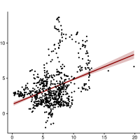
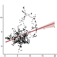
relu

leakyrelu

convex combination

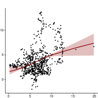
Note: This figure shows the nexus between inflation and money growth for the US and illustrates the functional forms of the activation functions specified in Table 1. The data for the consumer price index (i.e., CPIAUCSL) and money supply (i.e., M2SL) are taken from the FRED-MD database as described in McCracken and Ng (2016). We plot the following example: $y_{t}=f(x_{t})+\varepsilon_{t}$, where $y_{t}$ is the year-on-year inflation and $x_{t}$ is the $18^{th}$ lag of the year-on-year money supply growth (see Eq. (3)). $f$ refers to the activation functions specified in Table 1. The top-left panel ‘convex combination’ refers to our main specification, where we let the data decide on the form of the activation function.

2.3 The error variance

Neural networks often explicitly or implicitly assume that the error variance is constant. This assumption implies that the mean function explains a constant share of variation in $y_{t}$ over time. For macroeconomic data, this assumption is strong. In exceptional periods such as the global financial crisis (GFC) or the Covid-19 pandemic mean relations change and the explanatory power of certain elements in $\bm{x}_{t}$ might deteriorate. As a solution, we model the error variance in a time-varying manner using a standard stochastic volatility model.

Our model assumes that $\nu_{t}=\log\sigma_{t}^{2}$ evolves according to an AR(1) process:

$$\nu_{t}=\mu_{\nu}+\rho_{\nu}(\nu_{t-1}-\mu_{\nu})+\varsigma_{t},\quad\varsigma_{t}\sim\mathcal{N}(0,\xi_{\nu}^{2}),$$ (4)

with $\mu_{\nu}$ denoting the long-run level of the log-volatility, $\rho_{\nu}$ the persistence parameter and $\xi_{\nu}^{2}$ the state equation variance. This model assumes that the error variance evolves smoothly over time (if $\rho_{\nu}$ is close to 1) and feature their own shock. For later convenience, we let $\bm{\nu}=(\nu_{1},\dots,\nu_{T})^{\prime}$ denote the full history of the log-volatilities and $\bm{\beta}_{\nu}=(\mu_{\nu},\rho_{\nu},\xi_{\nu}^{2})^{\prime}$ the parameters of the log-volatility state equation.

2.4 The posteriors

In general, posterior inference in neural networks is extremely challenging. We tackle some of the issues by proposing a Markov Chain Monte Carlo (MCMC) algorithm that exploits the fact that the effective number of neurons $Q^{*}$ is often much smaller than $Q$. If this is the case, the corresponding parameters $\bm{\kappa}_{q}$ do not impact the likelihood of the model and hence we can easily simulate them from the prior. Since sampling the $\bm{\kappa}_{q}$s is typically achieved through variants of the Metropolis Hastings (MH) algorithm and this constitutes the main source of mixing issues in this general class of models, our approach reduces this problem by relying on HMC techniques and, second, by building on the literature on approximate Bayesian computation and assuming that if the amount of shrinkage introduced through the MGP prior on the $j^{th}$ neuron becomes large, we can safely ignore the relevant neuron and replace the MH updating step by simply drawing from the prior (which is trivial). In our experiments, we find that this approach works extremely well and yields predictive densities which are very close to the exact ones.

At a general level, we obtain draws from the joint posterior distribution using an MCMC algorithm that cycles between the following steps (with exact details on the full conditional posterior distributions provided in Sub-section A.1 in the appendix):

• Both the linear coefficients $\bm{\gamma}$ and the weights $\bm{\beta}$ associated with the neurons are obtained jointly from a standard multivariate Gaussian posterior, see Eqs. (A.1) and (A.2).

• For shrinking the linear coefficients, we use the horseshoe prior (Carvalho et al., 2010) and update the corresponding hyperparameters by sampling from inverse Gamma distributions using the auxiliary sampler proposed in Makalic and Schmidt (2015), see Eqs. (A.3) to (A.6).

• The hyperparameters associated with the MGP prior are obtained through simple Gibbs updating steps, see Eqs. (A.7) to (A.8).

• Sampling from $p(\bm{\kappa}_{q}|\bullet)$, for $q=1,\dots,Q$, is achieved as follows:

  • If the corresponding scaling parameter of the MGP prior exceeds a threshold very close to zero, we sample $\bm{\kappa}_{q}$ using an Hamiltonian Monte Carlo (HMC) step, see Eqs. (A.9) to (A.13).

  • Otherwise, $\bm{\kappa}_{q}$ is obtained by drawing from the prior.

• The shrinkage hyperparameters of the horseshoe prior on $\bm{\kappa}_{q}$ are obtained from simple inverse Gamma posteriors, see Eqs. (A.14) to (A.17).

• The function $h_{q}$ is simulated by first introducing an indicator $\delta_{q}$ which takes integer values one to four and indicates the precise function chosen. This indicator is then simulated from a multinomial distribution, see Eq. (A.18), and the relevant functional form of the activation function is chosen.

• Draws of $\bm{v}$ and $\bm{\beta}_{v}$ are simulated using the algorithm proposed in Kastner and Frühwirth-Schnatter (2014).

We iterate through our MCMC algorithm 20,000 times and discard the first 10,000 draws as burn-in. Information on the MCMC mixing properties of our sampler is provided in Sub-section B.4 in the appendix.

3 Simulation exercise

3.1 Design of the simulation exercise

In this section, we illustrate our approach through synthetic data, generated from either a linear or a nonlinear data generating processes (DGP). Our nonlinear DGP is defined as a neural network with a single hidden layer and a randomly selected activation function for each neuron (with an equal probability between the functions listed in Table 1). In addition, we assume that each neuron is informed by a single covariate in $\bm{x}_{t}$. In general, our DGP assumes that:

$$y_{t}= f(\bm{x}^{\prime}_{t}\bm{\kappa}_{true})^{\prime}\bm{\beta}_{true}+v_{t},\quad v_{t}\sim\mathcal{N}(0,\sigma^{2}_{t,true}),\quad\bm{\kappa}_{true}=\bm{I}_{K},$$ (5)

$$x_{jt}\sim \mathcal{N}(0,1),\text{ for }j=1,\dots,K\text{ and }K\in[30,60],$$ (6)

where $f:\mathbb{R}^{K}\mapsto\mathbb{R}^{Q}$. The number of neurons $Q(=K)$ is set to imply a medium-scale network ($Q=30$) or a rather large one ($Q=60$). The $Q$-dimensional vector of linear coefficients $\bm{\beta}_{true}$ allows us to distinguish between a truly sparse and a truly dense specification. Elements in $\bm{\beta}_{true}$ are defined according to $\beta_{j,true}\sim N(0,c^{2})$, with $c^{2}=0.5$. In the dense model 90 percent of the neurons are active whereas in the sparse specification only one out of ten neurons gets a non-zero weight. For the variance of the error term, we additionally differentiate between a homoskedastic ($\sigma^{2}_{t,true}=0.1$ for all $t$) and a heteroskedastic ($\sigma^{2}_{t,true}=0.1\exp{(\eta_{t})}$, with $\eta_{t}\sim N(0,0.01)$) specification.

To investigate the performance of the model we carry out a forecasting exercise using synthetic data. We simulate data of length $T=200$ and use $100$ randomly selected observations to train the different models. Forecast distributions are then computed for the remaining $100$ periods in $20$ replications. For the simulation exercise, moreover, we set the autoregressive coefficient of the SV process in Eq. (4) to zero to remove any time dependence. Thus, all 100 predictions can be obtained independently in a single sweep. In our simulations we consider the Bayesian NN with an activation function common to all neurons (labeled BNN), and the BNN where each neuron features its own activation function (labeled BNN-NS). The benchmark is the linear model with a horseshoe prior and SV, which typically performs very well in forecasting applications.

3.2 BNN forecasting performance with simulated data

Table 2 summarizes the forecasting performance of our BNNs for the DGPs featuring SV. It reports the root mean squared errors (RMSEs) of BNN and BNN-NS relative to the linear model, so that a relative RMSE smaller than one indicates over-performance with respect to the linear model. To investigate the tail forecasting performance within a controlled environment, the parentheses below the relative RMSEs include the 25th and 75th quantile scores (QSs) relative to the linear model, so that values smaller than unity indicate outperformance of the corresponding nonlinear model.

Overall, Table 2 suggests that for the nonlinear DGP the BNN-NS significantly outperforms the linear model for both the point and the tail forecasts, while BNN is comparable (which confirms the good forecasting capability of a linear model when complemented with the horseshoe prior and SV). Interestingly, for the linear DGP, the forecast accuracy of both BNN models is quite similar to that of the benchmark model (i.e., relative RMSEs and QSs are close to one). Hence, the extra flexibility of the BNN does not adversely affects its predictive accuracy if the true model is linear, while it helps if the true model is non-linear, more so for BNN-NS.

Zooming in on the different versions of the nonlinear DGP, it turns out that the relative performance of BNN and BNN-NS generally improves for the homoskedatic DGPs (with the exception of $K$=60 and the sparse DGP where there are little differences), and the absolute performance of the linear model improves as well. Moreover, when $K$=30, BNN and BNN-NS are better with the sparse DGPs than with the dense ones. This is partly due to the much worse absolute performance of the linear model with the sparse DGPs. When instead $K$=60, the relative performance of BNN and BNN-NS is better for the dense DGPs, and the linear models do even worse in absolute terms for the sparse DGPs. Therefore, when the number of regressors is large, sparsity creates complications for both the nonlinear and the linear models, but more so for the latter. Finally, the absolute performance of the linear model deteriorates with sparsity also with the linear DGP, but much less than with the nonlinear DGP. With the former, the relative performance of BNN and BNN-NS is instead rather stable across specifications and number of regressors, and comparable to that of the linear model, as already mentioned.

Table 2: Synthetic. Point forecast performance for 100 hold-out observations (estimated with SV).

K	Sparsity	Noise		Non-linear DGP				Linear DGP
				BNN	BNN-NS	Linear model		BNN	BNN-NS	Linear model
30	Dense	hetero		1.00	0.93	0.51		1.01	1.01	0.43
				(1.00),(1.00)	(0.93),(0.95)	(0.65),(0.64)		(1.01),(1.00)	(1.01),(1.00)	(0.46),(0.51)
		homo		0.99	0.86	0.41		1.02	1.02	0.32
				(0.97),(0.96)	(0.83),(0.85)	(0.51),(0.48)		(1.02),(1.01)	(1.02),(1.01)	(0.34),(0.34)
	Sparse	hetero		0.99	0.80	0.98		0.99	0.99	0.49
				(0.98),(1.01)	(0.77),(0.82)	(1.07),(1.10)		(1.00),(1.00)	(1.00),(0.99)	(0.50),(0.48)
		homo		0.98	0.72	1.00		1.01	1.01	0.35
				(0.98),(0.99)	(0.71),(0.68)	(1.07),(1.11)		(1.01),(1.00)	(1.00),(1.00)	(0.35),(0.34)
60	Dense	hetero		1.00	0.89	0.61		1.00	1.00	0.42
				(1.00),(1.00)	(0.90),(0.89)	(0.72),(0.71)		(0.99),(1.00)	(0.99),(1.00)	(0.46),(0.45)
		homo		1.01	0.84	0.54		1.01	1.01	0.33
				(1.01),(1.00)	(0.81),(0.85)	(0.62),(0.60)		(1.01),(1.01)	(1.02),(1.01)	(0.34),(0.32)
	Sparse	hetero		0.99	0.92	1.48		0.98	0.99	0.51
				(1.00),(1.00)	(0.91),(0.93)	(1.62),(1.68)		(0.98),(0.99)	(0.98),(0.99)	(0.55),(0.51)
		homo		1.00	0.94	1.37		1.01	1.00	0.38
				(0.99),(1.00)	(0.93),(0.95)	(1.48),(1.55)		(1.01),(1.03)	(1.00),(1.00)	(0.38),(0.37)

Note: The table shows root mean squared errors (RMSEs) relative to the benchmark linear model. The numbers in parentheses show the 25/75 quantile scores. In bold we mark the best performing model for each case. The grey shaded area gives the actual RMSE scores of the benchmark. Results are averaged across the hold-out.

4 Empirical Applications

We now consider the performance of the BNN models in four different topical empirical applications, see Sub-section 4.1 and the summary in Table 3 for more details, and carry out extensive forecasting exercises in Sub-section 4.2. These allow us to assess whether, from a predictive viewpoint, allowing for nonlinearities of an unknown form is preferable relative to simpler model specifications. We also include in the set of competing models a neural network estimated by backpropagation (labeled BNN-BP, described in Sub-section A.2 in the appendix) and an alternative very flexible nonparametric specification, Bayesian additive regression trees (BART, see e.g. Chipman et al. (2010) and Sub-section A.3 in the appendix), to assess whether or not our BNN specification can outperform it. In Sub-section 4.3 we investigate the role of the various activation functions / types of nonlinearity. In Sub-section 4.4 we focus on the effective number of neurons, as a summary measure of model complexity and in Sub-section 4.5 we relate the in-sample and out-of-sample results. Finally, in Sub-section 4.6 we discuss the performance of our BNN specification when adding additional layers to the network. Section B.2 in the appendix presents additional results related to the relative performance of each model for each dataset, also assessing the statistical significance of the differences in RMSE and log predictive likelihood (LPL) by means of the Diebold and Mariano (1995) test.

4.1 The four applications

In this sub-section, we provide details on the different applications and the datasets involved.

Macro A: modeling and forecasting key macroeconomic variables. The first application focuses on modeling and forecasting key US macroeconomic variables, using the popular FRED-MD database proposed in McCracken and Ng (2016). To gain a comprehensive picture of the importance of nonlinearities in large macro datasets, our forecasting exercise includes the consumer price (CPIAUCSL) inflation rate as specified in Stock and Watson (1999) and labeled as Macro A.1, the monthly growth rate of industrial production (INDPRO), labeled as Macro A.2, and the monthly growth rate of employment (CE16OV), labeled as Macro A.3. The sample ranges from January 1960 to December 2020 and includes 120 economic and financial variables for the large covariate set. We present results obtained from estimation based on smaller sets of variables in the appendix.

We compute the one-month-ahead predictive distributions for our hold-out sample, which starts in January 2000 and ends in December 2020 (i.e., $252$ monthly hold-out periods). These forecasts are obtained recursively, meaning that we use the data through January 2000 as a training sample and then forecast one-month-ahead. After obtaining the corresponding predictive densities, the sample is expanded by a single month. This procedure is repeated until the end of the sample is reached.

Macro B: long-term economic growth in a cross-section of countries. In the second application we study the presence of nonlinearities using the standard cross-sectional dataset proposed in Barro and Lee (1994). This dataset comprises a wide range of cross-country characteristics over the period 1960 to 1985. As dependent variable, we model the average growth rate of GDP per capita and regress it on the initial level of the exogenous variables to avoid endogeneity issues (Barro and Lee, 1994).

To investigate the extent of nonlinearities, we randomly pick 45 countries and predict the remaining $45$ countries. This is repeated $100$ times. Since flexible models should do better in the tails, we also consider a case in which our hold-out includes only countries with GDP growth rates outside the $25^{th}$ and $75^{th}$ percentiles (i.e., countries with very low/very high growth rates of GDP per capita).

Macro C: modeling and forecasting quarterly exchange rate returns. The recent literature on forecasting exchange rates suggests that accounting for nonlinearities increases predictive accuracy and helps to outperform simple benchmarks such as the random walk (see, e.g., Wright, 2008; Rossi, 2013; Huber and Zörner, 2019; Beckmann et al., 2020). We investigate this claim more carefully and forecast the USD/GBP exchange rate using our set of models. We construct a medium-sized application using a kitchen sink regression with 19 fundamentals including macroeconomic variables (i.e., unemployment rate and real GDP), price indices (i.e., producer and consumer price index as well as the oil price), short- and long-term interest rates, monetary supply measures and stock market variables (i.e., S&P 500 and VIX). Additional results based on smaller, theoretically motivated models can be found in the appendix.

Our sample starts in the first quarter of 1990 and ends in the last quarter of 2019. We again use a recursive forecasting design and focus on one- and four-steps-ahead predictions. The initial training sample ranges from $1990$Q$1$ to $1999$Q$1$. The remaining observations are left for forecast validation (i.e., $80$ quarterly observations).

Finance: forecasting the equity premium. In our finance application we assess the effect of controlling for nonlinearities on estimating and predicting US aggregate stock returns. We use the dataset described in Welch and Goyal (2008) which includes 16 predictors covering macroeconomic as well as interest rates and stock market variables. The variable to predict is the US equity premium measured by the continuously compounded returns on the S&P 500 index. The sample spans the period 1948 to 2020 at a yearly frequency. Our hold-out starts in 1965 and ends in 2020 (i.e., $56$ yearly observations). It is worth stressing that our forecast design implies a small number of observations in the initial traning sample. This serves to illustrate how neural networks learn in light of very short time series.

Table 3 summarizes the applications, provides information on the datasets, the sample and additional details on the forecasting exercises.

Table 3: Empirical applications.

	Dependent variable	Set of predictors	Sample	Range	Horizon	Hold-out	Source/reference
Macro A	A.1) Industrial production A.2) Inflation A.3) Employment	Large (120 economic & financial variables)	Monthly data for the US	1960M1 to 2020M12	one-step-ahead	2000M1 to 2020M12	McCracken and Ng (2016)
Macro B	Average economic growth rate	60 country-specific characteristics	Cross-section	90 countries	100 random samples	45 countries	Barro and Lee (1994)
Macro C	USD/GBP exchange rate returns (qoq)	20 exchange rate determinants	Quarterly data for the US and UK	1990Q1 to 2019Q4	one-step- and four-steps-ahead	2000Q1 to 2019Q4	Wright (2008); Rossi (2013)
Finance	Equity premium	16 economic & financial variables	Annual data for the US	1948 to 2020	one-year-ahead	1965 to 2020	Welch and Goyal (2008)

Note: The table gives an overview of the different empirical applications with which we test our proposed Bayesian neural network approach and present results in Sub-section 4.2. For more details on all datasets used for evaluating the performance of our BNNs we refer to Sub-section B.1 in the appendix.

4.2 Out-of-sample predictive accuracy

In this section we present the main forecasting results. For all four applications we focus on one particular dataset (Large for Macro A, all 20 determinants for Macro C and all 16 variables for Finance) and the one-step-ahead horizon. Results for the other smaller datasets and higher-order forecasts for Macro C are provided in Section B.2 in the appendix. For the former, the forecasting performance is often worse (or not better) than that based on the large dataset, indicating that large information sets matter also when included in nonlinear models.

Figure 2: Cumulative LPLs against the benchmark for the one-step-ahead predictive densities.

Macro A.1: Inflation

Macro B: GDP per capita growth

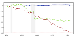
Macro A.2: Industrial production

Macro C: USD/GBP exchange rate

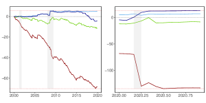
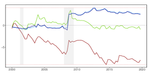
Macro A.3: Employment

Finance: S&P 500 excess returns

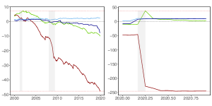
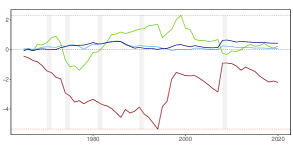
Note: For the time series applications we plot the evolution of cumulative log predictive likelihoods (LPLs) against the benchmark for the one-step-ahead predictive densities. Here, we choose the linear model of each specification as our benchmark to highlight the effect of controlling for nonlinearities. Note that this is in contrast to the tables in Section B.2 in the appendix where we choose a global benchmark for each application. The red dashed lines denote the max./min. LPLs at the end of the hold-out sample, while the gray shaded areas indicate the NBER recessions. For Macro B we plot relative LPLs against the linear model. The red dashed lines denote the max./min. LPLs.

Figure 2 shows cumulative one-step-ahead LPLs relative to the linear benchmark model over time and across all empirical applications considered, except for Macro B for which the LPLs are not cumulated, with positive values indicating that the nonlinear models are better than the linear benchmark.

We start our discussion with the results for the Macro A dataset (Macro A.1 - Macro A.3). Across all three target variables we find that during recessions (and the pandemic) the BNNs yield more accurate density predictions than the linear model. Focusing on the period before the Covid-19 pandemic for all three focus variables under consideration a single best performing model emerges: the BNN with a common activation function. The flexible BNN with neuron-specific activation functions also produces good inflation forecasts while it performs slightly worse for industrial production and employment. In these two cases it is outperformed by the linear benchmark model with SV (at least before the global outbreak of the pandemic in March 2020).

Zooming into the different focus variables reveals some interesting patterns over time. For inflation, in general, we find that both BNNs provide good density predictions during and after the GFC. Higher predictive accuracy is typically observed during episodes of deflationary pressures. While we find for pre-pandemic output forecasts (as measured by industrial production) that the nonlinear BNNs perform well during the GFC, we do not find these gains in accuracy for employment; instead, we observe a steady decline in relative cumulative LPLs starting in late 2005. When focusing on the pandemic period for both real economic activity variables, however, we observe a remarkable improvement in the forecasting performance of the BNN-NS model, which outperforms all other competitors in March 2020 and finally at the end of the hold-out sample. This observation provides evidence that a high degree of model flexibility, and thus capturing these severe outliers in real economic activity, pays off in terms of predictive accuracy. These large gains in forecast accuracy are not evident for inflation, which remained rather stable relative to industrial production and employment in 2020 and did not exhibit these severe outliers.

Finally, the worst performing model is also consistent across target variables: the BNN-BP. The dismal performance of BNN-BP is driven by too narrow predictive bounds. This claim is evidenced by the fact that BNN-BP performs poorly during extreme periods (with the slope of the relative LPL curves being negative and becoming much steeper). BART is also dominated by BNN for all variables and most sample periods, suggesting that BNN can provide an even more flexible specification, at least for these variables. Moreover, from the appendix (see, Table B.3), it turns out that BNN works well with respect to the linear model also in terms of point forecasts, with slightly better or comparable performance for all variables .

Since the LPL gains from the BNN specifications vary over time compared to the benchmark linear model, we also perform Giacomini and Rossi (2010) tests to assess whether or not the outperformance can be considered stable over time. Figure B.4 in the appendix reports the fluctuation test statistic for all models over the full hold-out period. The null hypothesis of stability is not rejected for all BNN specifications, except for the real economic activity variables during the Covid-19 period (i.e., Macro A.2 and Macro A.3). During the pandemic, we observe that BNN-NS significantly outperforms the benchmark for industrial production, while BNN-BP performs significantly worse in terms of predictive accuracy for both industrial production and employment.

Next we turn to the cross-sectional economic growth dataset (Macro B). Since this is a cross-section we do not show cumulative LPLs but, for each (randomly chosen) hold-out, the corresponding log predictive likelihood of the single best performing model (in this case BNN-NS) against the linear regression model. Notice that in this exercise no model features stochastic volatility. When we randomly drop countries from the dataset and train the model based on the remaining countries, we obtain LPLs which are consistently much better than the ones of the linear benchmark. In the vast majority of hold-outs BNN-NS yields superior forecast densities. There is only a single random sample where the neural network with neuron-specific activation functions performs slightly worse than the linear model. When we focus on countries that display extreme average growth rates of income per capita, predictive gains become enormous (more so for BNN-NS than for the BNN with a common activation function, as shown in Figure B.1 the appendix).

The results based on the first two datasets suggest that our Bayesian variants of a neural network do particularly well when time series display sharp changes or observations are extreme. Exchange rate dynamics also share features such as sudden changes in the level and/or volatility clustering. Hence, nonlinear techniques should be well suited for producing accurate forecasts. This indeed comes out from the figure associated with Macro C. Early in the sample, the different BNNs are slightly worse than the linear benchmark (with BNN-BP, again, being substantially inferior). However, as time passes by, flexible models seem to become better and sharply improve upon the linear specification in late 2004 and during the GFC. In this specific example, BNN-NS and BNN exhibit a very similar predictive performance. Most of the gains from using a nonlinear model are again obtained during times of economic stress. In particular, the US dollar sharply appreciated vis-á-vis the pound during the GFC and all neural network models are quick to adapt to this pattern. Table B.5 in the appendix shows that in terms of RMSEs there are little or no gains from the various BNN specifications, confirming that the LPL gains do not come from the center of the distributions. Moreover, there are some LPL gains also at the one-year horizon, and each single fundamental driver is associated with very similar LPL gains (and no or very small RMSE gains).

Finally, we consider whether BNNs do well when forecasting yearly equity returns. While both the BNN and BNN-NS outperform the benchmark in the late 1970s and 1980s, predictive performance is more muted during the Great Moderation; however, we again observe sharp improvements in predictive accuracy during the GFC, in particular for BNN-NS. As opposed to previous datasets, we find that the nonparametric BART model performs extraordinary well until the GFC in 2008 (with a period of somewhat weaker predictive accuracy in the late 1970s and early 1980s). Among the individual predictors, Table B.6 in the appendix shows that we get gains both in terms of RMSE and LPL for all single drivers but the differences are rather small.

Collecting similarities across all four forecasting exercises yields a story that BNNs work well during recessionary episodes or when the target variable takes on extreme values (i.e. values that are located in the tails). This result holds irrespective of whether the data is monthly (and thus features much more high frequency variation), quarterly, yearly or if we focus on a cross-sectional dataset. The key question, which we are going to investigate in the next two sub-sections, is what determines this strong performance in the tails.

4.3 Which activation functions?

One of the questions that arises is which activation functions give rise to the good forecasts during extreme periods. We answer this by computing the posterior inclusion probability (PIP) that a given function is chosen by our algorithm. This is obtained by taking draws from the posterior of $\delta_{q}$ and then computing

$$Prob(\delta_{q}=m|\text{Data})=\frac{\sum_{s=1}^{S}(\delta_{q}=m)}{S},$$

where $S$ is the number of retained draws from the posterior. In case of the neuron-specific specification we report averages across neurons to simplify the exposition.

Figure 3: Choice of the activation function.

Macro A.1: Inflation

Macro B: GDP per capita growth

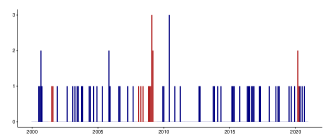
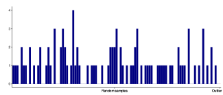
Macro A.2: Industrial production

Macro C: USD/GBP exchange rate

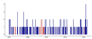
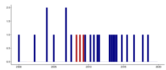
Macro A.3: Employment

Finance: S&P 500 excess returns

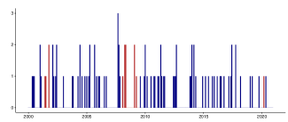
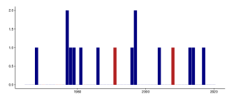
Note: This figure shows posterior inclusion probabilities (PIPs) over the hold-out period for the BNN with a common activation function for each dataset.

Figure 4 shows the PIPs of the different activation functions across datasets over the respective hold-out periods. Dark blue shaded cells imply that the corresponding activation function (in the rows of the heatmap) receives substantial PIP whereas white cells signal low PIPs of a respective activation function.

At a very general level, we find two patterns. The first relates to activation functions in our standard monthly macro dataset. Modeling industrial production, inflation and employment is best done with a neural network that features the sigmoid activation function for most of the hold-out period. Other activation functions receive less weight or a weight close to zero. There are distinct regimes (such as a brief period during the GFC in the case of CPI inflation and industrial production) where the PIPs change so as to attribute most posterior probability to the relu and leakyrelu activation function in the case of CPI inflation and the tanh activation function in the case of industrial production. This shift happens later for employment which seems to lag the business cycle (i.e. employment reached its trough much later than industrial production growth during the GFC). Here, we observe a mixture of the different activation functions until the outbreak of Covid-19 but a shift towards the sigmoid activation function for the subsequent periods. Notice that sigmoid and tanh underweight extreme values of $\bm{x}^{\prime}_{t}\bm{\kappa}_{q}+\zeta_{q}$, implying that if there is a switch in activation functions, we observe sharp changes in the dependent variable and this is captured through abrupt shifts in $f(\bm{x}_{t})$. This provides empirical evidence in favor of recent theoretical macro models that allow for nonlinearities, see for example Harding et al. (2022) for the case of inflation explained with a nonlinear Phillips curve.

Second, when we focus on the other macro datasets we observe less time variation in PIPs over the hold-out period and that sigmoid is not the dominant choice with most posterior weight anymore. For Macro B, two activation functions (tanh and sigmoid) receive all of the posterior mass with relu and leakyrelu never being included. A similar but more attenuated picture arises for Finance where tanh receives most posterior weight but also the other three activation functions share about 10 percent of posterior mass. Notice that for Finance the PIPs suggest that tanh receives most posterior weight between the mid 1970s and the late 1990s. Before and after that period, we also observe posterior mass on relu and leakyrelu. From Table 1, this implies that extreme values of variables such as dividend price ratios can have a much stronger effect on stock returns than values close to their sample mean. For Macro C, we find a mixture of all four activation functions. Relu and leakyrelu receive substantial posterior mass over the entire hold-out with tanh and sigmoid gaining in weight for the periods before the GFC and after 2015.

4.4 Effective number of neurons $Q^{\ast}$

In the previous sub-section we focused on which activation function (and thus form of nonlinearity) gives rise to the forecast distributions. This analysis, however, does not tell us anything about the quantitative relevance of the nonlinear part of the model. In this sub-section we will focus on whether the forecast distributions are generated by models that feature a large number of neurons (i.e. models that are highly nonlinear) or by models that feature few active neurons (i.e. models closer to the linear specification).

Figure 4: Active number of neurons.

Macro A.1: Inflation

Macro B: GDP per capita growth

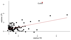
Macro A.2: Industrial production

Macro C: USD/GBP exchange rate

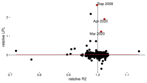
Macro A.3: Employment

Finance: S&P 500 excess returns

Note: This figure shows the number of significant neurons for the BNN with a common activation function and each application over the hold-out period. These are determined by computing the 5^th/ 95^th posterior credible intervals for each $\beta_{q}$ and if the credible intervals do not include zero the corresponding neuron is counted as being active a posteriori. In red we indicate the NBER recessions.

Figure 4 shows the number of active neurons for the different applications and over the hold-out period. A simple consideration of the axis scale reveals that, if any neuron is included, the number of neurons is rather low (ranging from two to four active neurons). This implies that rather simple forms of nonlinearities are often sufficient to explain the different datasets.

Focusing on the different applications we find that there is some heterogeneity with respect to the number of neurons over time. For Macro A, we find that in most periods, one or two active neurons are included. In (and around) recessions (indicated by the red bars), the number of neurons increases. This pattern is most pronounced during the GFC but also for the dotcom recession (e.g., employment) and the pandemic (see, inflation and industrial production).

For Macro B, nonlinearities are included for most random samples. The predictions are based on models that include one up to four neurons. Notice, however, that most samples only include a single neuron, indicating rather simple forms of nonlinearities. Similarly, for Macro C we observe that predictions have been mostly generated with a single active neuron (with two exceptions, which are the first quarter of 2004 and the fourth quarter of 2006). Moreover, we find signs of nonlinearities during the GFC (indicated again by the red bars).

Finally, S&P 500 excess return predictions are based on models that are linear or include one up to two neurons. Over time, there is some heterogeneity with respect to the number of neurons. In the late 1970s, one to two neurons are entering the model. During the 1980s and 1990s the predictions are based on the linear specification except for the early 1990s recession marked in red. The model also includes nonlinearities during the downturn in stock markets observed in the GFC and in 2017, a period in which the US Fed started to increase its policy rate for the first time since 2008.

4.5 The relationship between in-sample fit and out-of-sample predictability

The results up to this point tell a story that flexible models help in the tails, are competitive in normal times and, depending on the dataset, the nature of nonlinearities might be subject to structural breaks or a combination of different types of nonlinearities induced by different activation functions. In this sub-section we ask whether neural networks extract information from $\bm{x}_{t}$ that linear models can not exploit and how this impacts predictive accuracy (measured again through LPLs).

To achieve this, we compute the amount of variation explained through the conditional mean piece (labeled R2) of the best performing neural network for each application and the linear regression model. These R2s are computed recursively and put in relation to the corresponding $t$-by-$t$ LPL using a simple scatter plot. The scatter plots are provided in Figure 5. The horizontal line at zero implies that if a point is below zero, the linear regression model produces superior density forecasts whereas in the opposite case, the BNN is forecasting better. Points to the left of the vertical line (which stands at one) imply less explanatory power of the BNN whereas points to the right indicate that the conditional mean part of the BNN explains more of the variation in the response as the linear model.

Figure 5: Relative R2 against relative LPL

Macro A.1: Inflation

Macro B: GDP per capita growth

Macro A.2: Industrial production

Macro C: USD/GBP exchange rate

Macro A.3: Employment

Finance: S&P 500 excess returns

Note: This figure shows relative R2 versus relative log predictive likelihood (LPL) of the BNN with a common activation function against the linear model for each of our four applications. We color observations which feature high in-sample fit and high predictive accuracy relative to the benchmark.

Table 4: Measures for the in-sample and out-of-sample outperformance of the BNN against the linear benchmark.

	Macro A				Macro B	Macro C	Finance
		Inflation	Industrial prod.	Employment
Outperformance		52%	57%	61%	96%	50%	40%
Outperformance & higher R2		36%	30%	59%	90%	50%	38%
Robust correlation		0.79	0.013	0.058	0.407	0.032	0.015

Note: The table shows three different measures describing the relationship between in-sample fit and out-of-sample predictability. The measure “Outperformance” gives the share of relative LPL being positive (i.e., corresponding to the datapoints in the upper quadrants of Figure 5). The second measure “Outperformance & higher R2” gives the share of relative LPL being positive and a relative R2 above one (i.e., corresponding to the datapoints in the right-upper quadrants of Figure 5). The last measure gives the coefficients from a robust linear regression model regressing the relative R2 on the relative LPL for each application.

Two examples illustrate how the scatter plot can be interpreted. Points in the quadrant with R2$>1$ and LPL$>0$ represent situations where the BNN is extracting information from $\bm{x}_{t}$ that leads to a higher in-sample fit and this information pays off for density forecasts. If R2$\approx 1$ but LPL $>0$ both models explain a similar amount of in-sample variation but density forecasting performance of the BNN is superior. In this case, these differences are likely driven by higher order moments of the predictive distribution.

Analyzing the scatter plots in Figure 5 provides several insights. We find that for Macro A.1, inflation, several points lie in the high R2, positive LPL quadrant. This implies that the BNN provides a somewhat higher in-sample fit which often translates into slightly better out-of-sample LPLs, since the majority of points lie above the zero line.

This story carries over to predicting employment (Macro A.3). Most points are clustered to the right of the vertical line featuring relative R2 above one. However, one of the consistent patterns emerging from our forecasting exercise was that BNNs work much better during economic downturns. When we focus on the points far out in the north-eastern corner we find periods which are characterized by high R2s but also substantially higher LPLs. The first is January 2000 corresponding to the dotcom recession and the second is spring 2020 (i.e., March and April 2020) when employment numbers exhibited historic declines due to the Covid-19 pandemic. In these three months, the BNN was explaining up to 5 percent more in-sample variation than the linear model. This translated into much better LPLs.

For industrial production (Macro A.2) we find a slightly different picture. Most points are clustered around relative R2s close to unity and LPLs being positive. Notice that the first months of the pandemic as well as September 2008 during the GFC are marked as outliers. The latter corresponds to the month of the bankruptcy of Lehman brothers that led to sharp declines in stock markets and contractions in economic activity whereas the former marks the period characterized by the US adopting a large battery of containment measures such as social distancing and lock-downs. The fact that these months are located on the vertical line indicates that the in-sample fit was close to being the same as in the case of the linear model but LPLs are much higher. This suggests that the BNN does a better job in capturing these observations through higher order non-Gaussian features in the predictive distribution. Inspection of the relevant densities (not shown) reveals much heavier tails and thus a higher probability of capturing these large outliers.

For Macro B, the cross-section growth application, an interesting pattern emerges. All points are located to the right of the vertical line, indicating that the BNNs consistently explain more in-sample variation than their linear counterparts. This also leads to better LPLs for most random samples. Notice that the outlier sample (i.e. the one that includes only countries with extreme GDP per capita growth rates) are located far out in the north-east of the scatter plot. For this specific verification sample the neural network’s R2 is more than four times larger than the one of the benchmark and the LPL is over 6. This indicates that the neural network is capable of extracting information from the covariates in the dataset that would, if a linear approach is adopted, be lost. And this information seems to pay off for density forecasts.

Interestingly, a similar story arises if we consider Macro C and Finance. For exchange rate forecasting, the neural network always features larger R2s than the linear model and this often translates into superior LPLs. In 2008Q4, a quarter where the US dollar appreciated sharply against the pound, the BNN’s R2 was close to four times larger than the one of the linear regression model. This translated into a much better density prediction (with relative LPL of about three). Finally, for the finance dataset we find most points located in the area with a relative R2 above one. About half of the predictions feature a higher relative LPL at the same time. Again, this is most pronounced for the recessionary period in 2008.

Summing up this discussion, we find that in extreme cases, our BNNs perform better in terms of density forecasts and these improvements are often accompanied by a substantially larger in-sample fit. This is closely related to the benign overfitting phenomenon discussed in, e.g., Bartlett et al. (2020), which states that neural networks fit the data almost perfectly in-sample but also yield superior out-of-sample predictions.

4.6 Predictive accuracy of deep BNNs

So far, we remained mostly silent about the fact that in the machine learning literature, the workhorse is not a shallow neural network, but a deep neural network. Several recent papers on macroeconomic forecasting, however, document a rather weak performance of deep neural nets (Makridakis S., 2018), while often comparatively simple specifications, such as an AR($1$)/RW model (Stock and Watson, 2007), simple/shallow neural nets (Nakamura, 2005; Hauzenberger et al., 2022) or pruned tree models (Coulombe, 2020; Huber et al., 2020), perform extremely well for these datasets. Nonetheless, we wonder whether deepening a sophisticated Bayesian neural network (deep BNN) could further improve predictive accuracy for our four macroeconomic time series and cross-sectional applications.

A deep BNN with $L$ hidden layers implies that Eq. (2) can be generalized to:

$$f(\bm{x}_{t})\approx \left(h^{(L)}(\bm{\kappa}^{(L)^{\prime}}\hat{\bm{x}}_{t}^{(L-1)}+\bm{\zeta}^{(L)})\right)\bm{\beta},\quad\text{with}$$ (7)

$$\hat{\bm{x}}^{(l)}_{t}= h^{(l)}(\bm{\kappa}^{(l)^{\prime}}\hat{\bm{x}}^{(l-1)}_{t}+\bm{\zeta}^{(l)}),\quad\text{for }1\leq l\leq L-1.$$

Here, $\bm{\beta}$ again denotes a $Q(=K)\times 1$ vector of loadings while, for $l=\{1,\dots,L\}$, $h^{(l)}(\bullet)$ refers to a layer-specific (nonlinear) activation function common to all neurons $\bm{\kappa}^{(l)}$ and bias terms $\bm{\zeta}^{(l)}$ in the respective layer. In addition, for the first layer (i.e., $l=1$), we set $\hat{\bm{x}}^{(0)}_{t}=\hat{\bm{x}}_{t}$. While for a shallow BNN we assume neuron-specific activation functions for a single layer, for a deep BNN we assume layer-specific activation functions common to layer-specific neurons.

Table 5 presents the relative density forecast performance (in terms of LPLs) of a deep BNN with three hidden layers compared to a shallow BNN. Overall, we find that the deep BNN yields a similar forecasting performance than its shallow counterpart. For some extreme events, such as Covid-19 (in application Macro A), we observe very modest improvements when adding additional layers, while for our cross-section application (i.e., Macro B) we observe a slightly weaker relative performance. Furthermore, it is worth mentioning that for a deep BNN with three hidden layers, the computation time increases by a factor of $12$ on average across all applications. We therefore conclude that using a shallow but possibly wide BNN specification captures an adequate degree of nonlinearities in the data while still being computationally efficient.

Table 5: Deep BNN. Density forecast performance.

Application			Deep BNN
			with 3 hidden layers
Macro A	Inflation Industrial production Employment		0.00 -0.02 0.03
Macro B			-0.38
Macro C			0.02
Finance			-0.02

Note: The table shows log predictive likelihoods (LPLs) relative to the best performing shallow BNN. Results are averaged across the hold-out.

5 Conclusion

In this paper we developed techniques to flexibly estimate shallow neural networks with many neurons and various types of activation functions in a Bayesian framework, for either sparse or dense datasets. Using shrinkage and selection priors allows us to determine the appropriate network structure. This includes not only selecting the relevant number of neurons but also different activation functions during a specifically designed and highly efficient MCMC sampling. As an additional technical improvement, we allow for heteroskedasticity in the shocks. The resulting BNNs are then applied to synthetic data. We show that they (as expected) improve upon linear models if the DGP is nonlinear but even if the DGP is linear, our techniques yield precise forecasts that are competitive to the ones of the linear model.

In our empirical application we apply the models to four different datasets commonly used in macroeconomics and finance, both cross-sectional and time series, and with different temporal frequency. We carry out forecasting experiments and show that different variants of the BNNs work well overall but in particular during extreme periods (or in the tails). A simple analysis based on in-sample R2s and out-of-sample predictive likelihoods reveals that in these extreme cases, BNNs explain more in-sample variation and this is often accompanied by superior density forecasts. The possibility of using different activation functions and number of neurons over time / units in our enhanced BNNs also improves the forecasting performance. When considering a more sophisticated network structure with several layers, we find little predictive gains and sometimes even losses in our empirical applications, in addition to a many-fold increase in computational time, indicating that a shallow but flexible network structure can be sufficient for economic applications.

These results are relevant not only for the forecasting literature but also for policy making and for theoretical macro and finance, as they imply that nonlinearities and extreme events are pervasive and should be properly taken into account in the decision making process and when developing theoretical models.

Appendices

Appendix A Technical appendix

A.1 Full conditional posterior distributions

In the following, we provide details on the full conditional posterior distribution for the proposed Markov chain Monte Carlo (MCMC) algorithm outlined in Section 2.4.

• Let $\bm{\theta}=(\bm{\gamma}^{\prime},\bm{\beta}^{\prime})^{\prime}$ denote a ($K+Q$)-dimensional vector of parameters and $\tilde{\bm{x}}=(\tilde{\bm{x}}_{1}^{\prime},\dots,\tilde{\bm{x}}_{T}^{\prime})^{\prime}$ a $(K+Q)\times T$ matrix of neurons with element $\tilde{\bm{x}}_{t}=(\bm{x}_{t}^{\prime},h_{1}(\bm{x}_{t}^{\prime}\bm{\kappa}_{1}+\zeta_{1}),\dots,h_{Q}(\bm{x}_{t}^{\prime}\bm{\kappa}_{Q}+\zeta_{Q}))^{\prime}$. Moreover, we define $\bm{\Sigma}=\text{diag}(\sigma^{2}_{1},\dots,\sigma^{2}_{T})$ as a $T\times T$ matrix capturing the variances and $\underline{\bm{V}}_{\bm{\theta}}=\text{diag}(\bm{\phi}^{-1}_{\bm{\gamma}},\bm{\phi}^{-1}_{\bm{\beta}})$ where $\bm{\phi}^{-1}_{\bm{\gamma}}=(\phi^{-1}_{\gamma_{1}},\dots,\phi^{-1}_{\gamma_{K}})^{\prime}$ denotes the $K$ prior variances for the constant coefficients and we collect $\bm{\phi}^{-1}_{\bm{\beta}}=(\phi^{-1}_{\beta_{1}},\dots,\phi^{-1}_{\beta_{Q}})^{\prime}$ for the nonlinear coefficients. The joint parameter vector $\bm{\theta}$ is then obtained from a standard multivariate Gaussian posterior:

  $$\bm{\theta}|\bullet\sim\mathcal{N}\left(\overline{\bm{\theta}},\overline{\bm{V}}_{\bm{\theta}}\right),$$ (A.1)

  with

  $$\overline{\bm{V}}_{\bm{\theta}} =\left(\tilde{\bm{x}}^{\prime}\bm{\Sigma}^{-1}\tilde{\bm{x}}+\underline{\bm{V}}_{\bm{\theta}}^{-1}\right)^{-1},$$

  $$\overline{\bm{\theta}} =\overline{\bm{V}}_{\bm{\theta}}\tilde{\bm{x}}^{\prime}\bm{\Sigma}^{-1}\bm{y}.$$

• The prior on $\bm{\gamma}$ is Normal of the form:

  $$\gamma_{j}\sim\mathcal{N}(0,\phi^{-1}_{\gamma_{j}}),\quad\phi^{-1}_{\gamma_{j}}=\lambda^{2}_{\bm{\gamma}}\varphi^{2}_{\gamma_{j}},\quad\text{for }j=1,\dots,K.$$ (A.2)

  We use a horseshoe prior and rely on the hierarchical representation of Makalic and Schmidt (2015). The global and local shrinkage parameters, $\lambda^{2}_{\bm{\gamma}}$ and $\varphi^{2}_{\gamma_{j}}$, respectively, are obtained by introducing auxiliary random quantities which follow an inverse Gamma distribution:

  $$\varphi^{2}_{\gamma_{j}}|\bullet \sim\mathcal{G}^{-1}\left(1,c^{-1}_{\gamma_{j}}+\frac{\gamma^{2}_{j}}{2\lambda^{2}_{\bm{\gamma}}}\right),$$ (A.3)

  $$\lambda^{2}_{\bm{\gamma}}|\bullet \sim\mathcal{G}^{-1}\left(\frac{K+1}{2},d^{-1}_{\bm{\gamma}}+\sum^{K}_{j=1}\frac{\gamma^{2}_{j}}{2\varphi^{2}_{\gamma_{j}}}\right),$$ (A.4)

  $$c_{\gamma_{j}}|\bullet \sim\mathcal{G}^{-1}\left(1,1+\varphi^{-2}_{\gamma_{j}}\right),$$ (A.5)

  $$d_{\bm{\gamma}}|\bullet \sim\mathcal{G}^{-1}\left(1,1+\lambda^{-2}_{\bm{\gamma}}\right).$$ (A.6)

• We sample the hyperparameters associated with the MGP prior on $\bm{\beta}$ from inverse Gamma distributions:

  $$\delta_{1} \sim\mathcal{G}^{-1}\left(a_{1}+\frac{Q}{2},1+\frac{1}{2}\sum^{Q}_{q=1}(\phi_{\beta_{q}}\beta^{2}_{q})\right),$$ (A.7)

  $$\delta_{r} \sim\mathcal{G}^{-1}\left(a_{2}+\frac{Q-r-1}{2},1+\frac{1}{2}\sum^{Q}_{q=1}(\phi_{\beta_{q}}\beta^{2}_{q})\right).$$ (A.8)

• To efficiently update $\bm{\kappa}_{q}$ ($q=1,\dots,Q)$, we rely on a Hamiltonian Monte Carlo (HMC, Neal et al., 2011) within Gibbs step. Let $\bm{r}_{q}$ denote an auxiliary moment variable for each $\bm{\kappa}_{q}$, where each element is standard normal distributed, i.e., $\bm{r}_{q}\sim\mathcal{N}(\bm{0},\bm{I})$. Furthermore, let $\mathcal{L}(\bm{\kappa}_{q})=\log p(\bm{\kappa}_{q}|\bullet)$ define the log conditional posterior density of $\bm{\kappa}_{q}$. The fictitious Hamiltonian system of the conditional posterior density of $\bm{\kappa}_{q}$ is then given by

  $$\mathcal{H}(\bm{\kappa}_{q},\bm{r}_{q})=-\mathcal{L}(\bm{\kappa}_{q})+\frac{1}{2}\bm{r}_{q}^{\prime}\bm{r}_{q}.$$ (A.9)

  Since we view Eq. (A.9) as a Hamiltonian system, the negative log conditional posterior can be interpreted as a potential energy while the term associated with the moment variable can be interpreted as kinetic energy (see, e.g., Childers et al., 2022). We simulate the Hamiltonian dynamics of this system via the leapfrog integrator with the following proposals:

  $$\bm{r}_{q}^{\ast\ast} =\bm{r}_{q}^{(a)}+\frac{\epsilon}{2}\nabla_{\bm{\kappa}_{q}}\mathcal{L}(\bm{\kappa}_{q}^{(a)}),$$ (A.10)

  $$\bm{\kappa}_{q}^{\ast} =\bm{\kappa}_{q}^{(a)}+\epsilon\bm{r}_{q}^{\ast\ast},$$ (A.11)

  $$\bm{r}_{q}^{\ast} =\bm{r}_{q}^{\ast\ast}+\frac{\epsilon}{2}\nabla_{\bm{\kappa}_{q}}\mathcal{L}(\bm{\kappa}_{q}^{\ast}),$$ (A.12)

  where $\bm{\kappa}_{q}^{(a)}$ and $\bm{r}_{q}^{(a)}$ denote the previously accepted values, while $\nabla_{\bm{\kappa}_{q}}\mathcal{L}(\bm{\kappa}_{q})$ is the gradient of the log conditional posterior. The leapfrog method uses a discrete step size $\epsilon$ to generate a full-step proposal for $\bm{\kappa}_{q}$ (denoted by $\bm{\kappa}_{q}^{\ast}$) and half-step updates for the momentum $\bm{r}_{q}$ (denoted by $\bm{r}_{q}^{\ast\ast}$ for the first half-step update and $\bm{r}_{q}^{\ast}$ for the final proposal). We repeat the leapfrog method in $n=1,\dots,N$ steps.

  The HMC thus uses information of the gradient of the log conditional posterior distribution to propose a new $\bm{\kappa}_{q}$ which greatly improves mixing of the Markov chain. Note that the gradient of the log conditional posterior density can be obtained in a straightforward manner, as we consider only a set of activation functions with well-defined gradients for each neuron. The parameters to tune the HMC algorithm are the step size $\epsilon$ and the number of leapfrog steps $N$. We follow state-of-the-art methods and run the No U-Turn Sampler (NUTS) as proposed by Hoffman et al. (2014), which automatically adapts these tuning parameters during sampling.

  Finally, we evaluate the proposed and previously accepted values by means of a Metropolis accept/reject step and determine the acceptance probability $\eta_{q}$ for proposed $\bm{\kappa}_{q}^{\ast}$:

  $$\eta_{q}=\text{min}\left(1,\frac{\text{exp}(\mathcal{L}(\bm{\kappa}_{q}^{\ast})-\frac{1}{2}\bm{r}_{q}^{{}^{\prime}\ast}\bm{r}_{q}^{\ast})}{\text{exp}(\mathcal{L}(\bm{\kappa}_{q}^{(a)})-\frac{1}{2}\bm{r}_{q}^{{}^{\prime}(a)}\bm{r}_{q}^{(a)})}\right).$$ (A.13)

  Note that this step remains conceptually similar for the deep BNN outlined in Sub-section 4.6. In this case, we only need to iterate through all layers and also take into account the fact that the composite function of $L$ layers has different implications on the gradients of the layer-specific neurons.

• To achieve shrinkage in the neurons we apply a column-wise horseshoe prior on the elements of $\bm{\kappa}_{q}$. We follow Makalic and Schmidt (2015) and define auxiliary random quantities, which are used to obtain the global and local shrinkage parameters, $\lambda^{2}_{\bm{\kappa}_{q}}$ and $\varphi^{2}_{\kappa_{jq}}$. The (hyper)parameters follow an inverse Gamma distribution:

  $$\varphi^{2}_{\kappa_{jq}}|\bullet \sim\mathcal{G}^{-1}\left(1,c^{-1}_{\kappa_{j}q}+\frac{\kappa^{2}_{jq}}{2\lambda^{2}_{\bm{\kappa}_{q}}}\right),$$ (A.14)

  $$\lambda^{2}_{\bm{\kappa}_{q}}|\bullet \sim\mathcal{G}^{-1}\left(\frac{K+1}{2},d_{\bm{\kappa}_{q}}^{-1}+\sum^{K}_{j=1}\frac{\kappa^{2}_{jq}}{2\varphi^{2}_{\kappa_{jq}}}\right),$$ (A.15)

  $$c_{\kappa_{jq}}|\bullet \sim\mathcal{G}^{-1}\left(1,1+\varphi^{-2}_{\kappa_{jq}}\right),$$ (A.16)

  $$d_{\bm{\kappa}_{q}}|\bullet \sim\mathcal{G}^{-1}\left(1,1+\lambda^{-2}_{\bm{\kappa}_{q}}\right).$$ (A.17)

• For choosing the activation function $h_{q}$, we draw the indicator $\delta_{q}$ from a multinomial distribution of the following form:

  $$\text{Pr}(\delta_{q}=m|\bullet)\propto\omega_{qm}\times\exp\left\{-\frac{1}{2}\left(\bm{(}\hat{\bm{y}}_{q}-\bm{\mu}^{(m)}_{q})^{\prime}\bm{\Sigma}^{-1}(\hat{\bm{y}}_{q}-\bm{\mu}^{(m)}_{q})\right)\right\},\quad\text{for }m=1,\dots,4,$$ (A.18)

  where $\bm{\mu}^{(m)}_{q}=(\mu^{(m)}_{1q},\dots,\mu^{(m)}_{Tq})^{\prime}$ with elements $\mu^{(m)}_{tq}=\beta_{q}h^{(m)}_{q}(\bm{x}_{t}^{\prime}\bm{\kappa}_{q}+\zeta_{q})$.

A.2 Bayesian neural network by backpropagation (BNN-BP)

A Bayesian neural network estimated by backpropagation was introduced by Blundell et al. (2015). It serves as a variational inference scheme for learning the posterior distribution on the weights of a neural network. To do so, the approach maximizes the log-likelihood of the model subject to a Kullback-Leibler complexity term on the parameters and makes use of the reparameterization trick (Kingma and Welling, 2013) to obtain the posterior distribution of the weights with stochastic gradient descent.

The prior on the weights is specified as a scale mixture of two Gaussian densities with zero mean but differing variances. The first mixture component features a large variance ($\sigma^{2}_{1}=3$) providing a heavy-tailed distribution whereas the variance of the other component is set small ($\sigma^{2}_{2}=0.0025$) concentrating the weights a priori around zero. This setup is similar to a spike and slab prior (see, George and McCulloch, 1993) but with the same prior parameters for all the weights to allow for the optimization by stochastic gradient descent.

The hyperparameters are chosen in a cross validation exercise. For the cross-sectional datasets (i.e., Macro B and synthetic) we randomly split the data into equally sized training and test sets. We evaluate each model specification in 20 replications and use those yielding the lowest average RMSE for the final model. For the time series applications (i.e., Macro A, Macro C and Finance) we use a cross validation based on an expanding window time series split. Specifically, we use all observations up to the last 24 months for Macro A, 12 quarters for Macro C and 10 years for Finance before the start of our hold-out to train the model and then, after obtaining the predictive densities, add the next observation and recompute the model. We repeat this until we end up at the beginning of our hold-out and choose the specification with the lowest average RMSE. We train all models in 1000 epochs and use the MSE loss function, the ADAM optimizer and a learning rate of 0.01.

A.3 Bayesian additive regression trees (BART)

Bayesian additive regression trees (Chipman et al., 2010) are an alternative to BNNs to approximate the unknown function $f$. The idea is to consider the sum over a number of $Z$ regression trees. Formally, this boils down to:

$$f(\bm{x}_{t})\approx\sum^{Z}_{z=1}g_{z}(\bm{x}_{t}|\mathcal{T}_{z},\bm{\rho}_{z})$$ (A.19)

A single regression tree $g_{z}$ depends on two parameters, the tree structure given by $\mathcal{T}_{z}$ and the terminal node parameter $\bm{\rho}_{z}$. Following Chipman et al. (2010), we set $Z=250$ and build the prior on the tree structure upon a tree-generating stochastic process. This involves determining the probability that a given node is nonterminal, the selection of variables used in a splitting rule (to spawn left and right children nodes) and the corresponding thresholds. For the terminal node parameter we specify a conjugate Gaussian prior distribution with data-based prior variance. In particular, the specification centers prior mass on the range of the data while ensuring a higher degree of shrinkage if the number of trees is large. Details can be found in Chipman et al. (2010).

Appendix B Empirical appendix

B.1 Details on the data

Table B.1: Full set of empirical applications.

	Dependent variable	Set of predictors	Sample	Range	Horizon	Hold-out	Source
Macro A	A.1) Industrial production A.2) Inflation A.3) Employment	1) Medium (20 economic & financial variables) 2) Large (120 economic & financial variables) 3) PCA	Monthly data for the US	1960M1 to 2020M12	one-step- and three-steps-ahead	2000M1 to 2020M12	McCracken and Ng (2016)
Macro B	Average economic growth rate	60 country-specific characteristics	Cross-section	90 countries	100 random samples	45 countries	Barro and Lee (1994)
Macro C	USD/GBP exchange rate returns (qoq)	1) 20 exchange rate determinants	Quarterly data for the US and UK	1990Q1 to 2019Q4	one-step- and four-steps-ahead	2000Q1 to 2019Q4	Wright (2008); Rossi (2013)
		2) Interest rate differential
		3) Inflation differential
		4) Monetary fundamentals
		5) Taylor rule differential
		6) All fundamentals
Finance	Equity premium	1) 16 economic & financial variables	Annual data for the US	1948 to 2020	one-year-ahead	1965 to 2020	Welch and Goyal (2008)
	(i.e., S&P 500	2) Inflation
	excess returns)	3) Term spread
		4) Dividend yield
		5) Dividend price ratio

Note: The table gives an overview of the different empirical applications with which we test our proposed Bayesian neural network approach. We evaluate the performance of the model approach in each application through root mean squared errors (RMSEs) for point forecasts and log predictive likelihoods (LPLs) for density forecasts.

B.2 Overall forecasting results

In this sub-section we provide additional results on our thorough forecasting exercise for the four empirical applications. We present detailed point and density forecasting performance of the different models compared to the linear model measured by relative root mean squared errors (RMSEs) and log predictive likelihoods (LPLs), respectively, for each application and forecasting horizon in Table B.3 to Table B.6. Moreover, we show cumulative LPLs over the hold-out for each forecasting horizon and application in Figure B.1 to Figure B.3. Note that for the cross-sectional example, Macro B in Figure B.1, we plot log predictive likelihoods against the linear model for the two best performing models, i.e., the BNN and the BNN-NS.

Table B.2: Synthetic. Point forecast performance for 100 hold-out observations (estimated with homoskedastic error variances).

K	Sparsity	Noise		Non-linear DGP				Linear DGP
				BNN	BNN-NS	Linear model		BNN	BNN-NS	Linear model
30	Dense	hetero		1.01	0.94	0.51		1.02	1.02	0.43
				(1.01),(1.00)	(0.95),(0.95)	(0.66),(0.64)		(1.02),(1.02)	(1.02),(1.02)	(0.46),(0.51)
		homo		0.98	0.84	0.41		1.02	1.02	0.32
				(0.96),(0.98)	(0.80),(0.84)	(0.51),(0.48)		(1.02),(1.01)	(1.02),(1.01)	(0.34),(0.34)
	Sparse	hetero		1.01	0.84	0.98		1.02	1.01	0.49
				(0.99),(0.99)	(0.79),(0.85)	(1.07),(1.10)		(1.02),(1.02)	(1.01),(1.01)	(0.50),(0.49)
		homo		1.02	0.72	1.01		1.00	1.00	0.35
				(1.00),(1.02)	(0.71),(0.68)	(1.07),(1.11)		(1.00),(1.00)	(1.00),(1.00)	(0.36),(0.34)
60	Dense	hetero		1.01	0.87	0.61		1.02	1.02	0.43
				(1.00),(1.00)	(0.87),(0.87)	(0.72),(0.71)		(1.02),(1.03)	(1.01),(1.02)	(0.46),(0.45)
		homo		1.01	0.85	0.53		1.01	1.01	0.33
				(1.01),(1.00)	(0.83),(0.86)	(0.62),(0.60)		(1.01),(1.01)	(1.01),(1.01)	(0.34),(0.32)
	Sparse	hetero		1.00	0.93	1.48		1.01	1.01	0.51
				(0.99),(1.00)	(0.89),(0.91)	(1.62),(1.68)		(1.01),(1.01)	(1.00),(1.01)	(0.56),(0.51)
		homo		1.01	0.95	1.38		1.01	1.01	0.38
				(0.98),(1.00)	(0.91),(0.94)	(1.49),(1.55)		(1.01),(1.01)	(1.01),(1.01)	(0.38),(0.37)

Note: The table shows root mean squared errors (RMSEs) relative to the benchmark linear model. The numbers in parentheses show the 25/75 quantile scores. In bold we mark the best performing model for each case. The grey shaded area gives the actual RMSE scores of the benchmark. Results are averaged across the hold-out.

Table B.3: Macro A. Forecast performance across 252 hold-out observations (one-month-ahead).

Covariates		Model
		BART	BNN	BNN-BP	BNN-NS	Linear model
Inflation
AR(1)		1.11***	1.05	1.03	1.05	1.05
		(-0.22***)	(-0.01)	(-0.19***)	(-0.01)	(-0.03)
Large		0.97	0.94***	1.03	0.94***	0.94***
		(-0.03)	(0.09***)	(-0.12***)	(0.08***)	(0.08***)
Medium		1.04	0.97	1.04**	0.97*	0.98
		(-0.10*)	(0.06***)	(-0.12***)	(0.04*)	(0.06***)
PCA		1.07**	1.00	1.04*	1.01	1.16
		(-0.20***)	(0.00)	(-0.11***)	(-0.04***)	(-1.45)
Industrial production
AR(1)		0.89	0.91	0.92	0.91	0.91
		(-0.12)	(0.09*)	(-0.81)	(0.06)	(0.03)
Large		0.88	0.97***	0.93	1.02**	0.98***
		(0.08)	(0.14***)	(-0.41*)	(0.17**)	(0.12***)
Medium		0.88	0.97*	0.93	0.97**	0.99**
		(0.03)	(0.10***)	(-0.41*)	(0.14**)	(0.06***)
PCA		0.89	1.00	0.94	1.01	1.75
		(-0.01)	(0.05**)	(-0.46)	(0.07*)	(-1.33)
Employment
AR(1)		1.14**	1.01	1.01	1.02	1.02
		(-0.67)	(0.11)	(-0.96)	(0.11)	(-0.07*)
Large		1.04	1.00	1.01	1.00	1.01
		(0.11)	(0.14**)	(-0.87)	(0.14)	(0.10*)
Medium		1.05	0.99	1.01	0.99	1.00
		(-0.28)	(0.14)	(-0.97)	(0.00)	(0.04)
PCA		1.03	0.99	1.01	1.00	3.50
		(-0.19*)	(0.07)	(-0.59)	(-0.01)	(-1.88)

Note: The table shows root mean squared errors (RMSEs), and average log predictive likelihoods (LPLs) in parentheses, relative to the linear benchmark. In bold we mark the best performing model for each case. The grey shaded area gives the actual RMSE and LPL scores of our benchmark (linear model). Asterisks indicate statistical significance by means of the Diebold and Mariano (1995) test for each model relative to the benchmark at the 1% (***), 5% (**) and 10% (*) significance levels. Results are averaged across the hold-out.

Table B.4: Macro B. Forecast performance across 45 hold-out countries and 100 replications.

Covariates		Model
		BART	BNN	BNN-BP	BNN-NS	Linear model
Kitchen sink		0.95***	1.01	1.04***	1.01	5.24
		(0.06***)	(0.82***)	(-0.18***)	(0.95***)	(-4.40)

Note: The table shows root mean squared errors (RMSEs), and average log predictive likelihoods (LPLs) in parentheses, relative to the linear benchmark. In bold we mark the best performing model for each case. The grey shaded area gives the actual RMSE and LPL scores of our benchmark (linear model). Asterisks indicate statistical significance by means of the Diebold and Mariano (1995) test for each model relative to the benchmark at the 1% (***), 5% (**) and 10% (*) significance levels. Results are averaged across the hold-out.

Table B.5: Macro C. Forecast performance across 80 hold-out observations.

Covariates		Multivariate models
		BART	BNN	BNN-BP	BNN-NS	Linear model
					one-quarter-ahead
All fundamentals		1.03	1.02	1.03	1.02	1.01
		(-0.02)	(0.01)	(-0.09*)	(0.02)	(-0.01)
Kitchen sink		1.04	0.97	1.02	0.99	0.95
		(-0.01)	(0.03)	(-0.10)	(0.03)	(-1.29)
					one-year-ahead
All fundamentals		1.04	1.00	1.01	1.00	1.00
		(0.00)	(0.02)	(-0.09**)	(0.00)	(-0.01)
Kitchen sink		1.03	1.01	0.98**	1.02	0.96
		(0.06)	(0.01)	(-0.09)	(0.01)	(-1.29)
		Univariate models
		BART		BNN-BP	BNN-NS	Linear model
					one-quarter-ahead
AR(1)		0.97		0.99	0.95***	0.96***
		(0.04)		(-0.06)	(0.06)	(0.05***)
Inflation differential		1.07		1.01	1.02	1.02
		(-0.01)		(-0.07)	(0.02)	(0.00)
IR differential		0.99		1.02	1.00	1.00
		(0.00)		(-0.08*)	(0.01)	(0.00)
Monetary fundamentals		1.06		1.00	1.00	1.01
		(-0.04)		(-0.07)	(0.02)	(0.01)
Taylor rule differential		1.09		1.01	1.01	1.01
		(-0.02)		(-0.08*)	(0.02)	(0.00)
					one-year-ahead
AR(1)		1.02		0.99	0.99	0.99
		(-0.01)		(-0.07**)	(0.02)	(0.00)
Inflation differential		1.03		0.99	1.00	0.99
		(0.00)		(-0.07**)	(0.02)	(0.00)
IR differential		1.04		1.01	0.99	0.99
		(0.01)		(-0.08**)	(0.02)	(-0.01)
Monetary fundamentals		1.00		1.00	0.99	0.99
		(0.01)		(-0.08**)	(0.02)	(0.00)
Taylor rule differential		1.06		1.01	1.00	0.99
		(-0.02)		(-0.09***)	(0.01)	(0.00)

Note: The table shows root mean squared errors (RMSEs), and average log predictive likelihoods (LPLs) in parentheses, relative to the linear benchmark. In bold we mark the best performing model for each case. The grey shaded area gives the actual RMSE and LPL scores of our benchmark (linear model). Asterisks indicate statistical significance by means of the Diebold and Mariano (1995) test for each model relative to the benchmark at the 1% (***), 5% (**) and 10% (*) significance levels. Results are averaged across the hold-out.

Table B.6: Finance. Forecast performance across 56 hold-out observations (one-year-ahead).

Covariates		Multivariate models
		BART	BNN	BNN-BP	BNN-NS	Linear model
Kitchen sink		1.00*	1.00	1.03	0.99	1.07
		(0.01)	(0.00)	(-0.04)	(0.01)	(-1.46)
		Univariate models
		BART		BNN-BP	BNN-NS	Linear model
Dividend price ratio		1.01		0.99	0.99	0.99
		(-0.04)		(0.00)	(0.00)	(-0.01)
Dividend yield		1.01		1.01	0.99	0.99
		(-0.02)		(-0.03)	(0.00)	(0.00)
Inflation		1.02		1.00	0.99	1.00
		(-0.02)		(0.00)	(0.01)	(0.00)
Term spread		1.00		0.99	1.01	0.99
		(-0.01)		(0.00)	(0.00)	(-0.01)

Note: The table shows root mean squared errors (RMSEs), and average log predictive likelihoods (LPLs) in parentheses, relative to the linear benchmark. In bold we mark the best performing model for each case. The grey shaded area gives the actual RMSE and LPL scores of our benchmark (linear model). Asterisks indicate statistical significance by means of the Diebold and Mariano (1995) test for each model relative to the benchmark at the 1% (***), 5% (**) and 10% (*) significance levels. Results are averaged across the hold-out.

Figure B.1: Macro B. LPLs against the benchmark.

BNN

BNN-NS

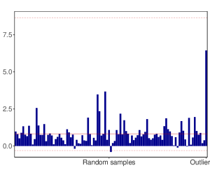
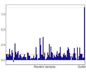
Note: This figures shows relative log predictive likelihoods (LPLs) against the linear model. The red dashed lines denote the max./min. LPLs and the red solid line indicates the mean.

Figure B.2: Macro C. Evolution of cumulative LPLs against the benchmark.

(a) one-quarter-ahead

Kitchen sink

All fundamentals

AR(1)

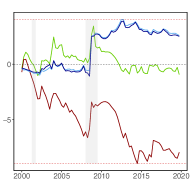
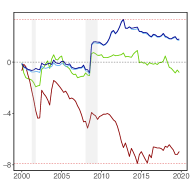
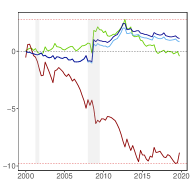
(b) one-year-ahead

Kitchen sink

All fundamentals

AR(1)

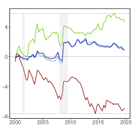
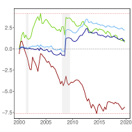
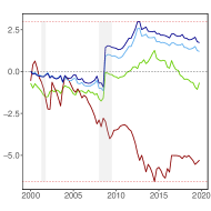
Note: This figure shows cumulative log predictive likelihoods (LPLs) against the benchmark for each specification. Here, we choose the linear model of each specification as our benchmark to highlight the effect of controlling for nonlinearities. Note that this is in contrast to the tables where we choose a global benchmark for each application. The red dashed lines denote the max./min. LPLs at the end of the hold-out sample, while the gray shaded areas indicate the NBER recessions.

Figure B.3: Finance. Evolution of cumulative LPLs against the benchmark.

Kitchen sink

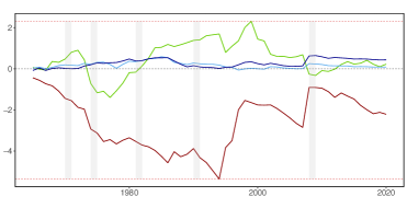
Inflation

Term spread

Dividend yield

Dividend price ratio

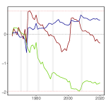
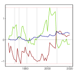
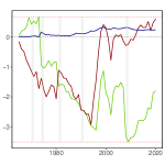
Note: This figure shows cumulative log predictive likelihoods (LPLs) against the benchmark for each specification. Here, we choose the linear model of each specification as our benchmark to highlight the effect of controlling for nonlinearities. Note that this is in contrast to the tables where we choose a global benchmark for each application. The red dashed lines denote the max./min. LPLs at the end of the hold-out sample, while the gray shaded areas indicate the NBER recessions.

B.3 Fluctuation tests

To test whether the outperformance presented in Figure 2 is stable over time, we calculate the fluctuation test statistic as proposed by Giacomini and Rossi (2010). Again, the linear model with the horseshoe prior serves as the benchmark in each application. We choose the 5 percent level for statistical significance. Positive values of the fluctuation test statistic imply that the corresponding model outperforms the benchmark. If model performance is inferior the test statistic gives negative values. Results are presented in Figure B.4.

Figure B.4: Fluctuation test statistic for the one-step-ahead density forecast performance.

Macro A.1: Inflation

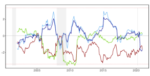
Macro A.2: Industrial production

Macro C: USD/GBP exchange rate

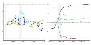
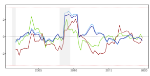
Macro A.3: Employment

Finance: S&P 500 excess returns

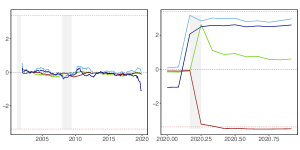
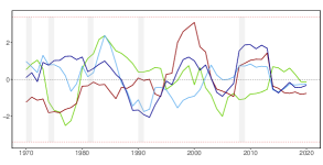
Note: This figure shows the fluctuation test statistic relative to the benchmark as proposed by Giacomini and Rossi (2010). Dashed lines indicate critical values for a 5% level of statistical significance. Positive values of the fluctuation test imply that the corresponding model outperforms the benchmark.

B.4 MCMC diagnostics of posterior estimates

For the most flexible specification, the BNN-NS model, we analyze the convergence properties of our algorithm by means of inefficiency factors (IF) and the Raftery and Lewis (1992) diagnostics. The former is determined by the inverse of the relative effective sample size. The latter counts the number of draws taken from the algorithm which are necessary to reach a certain level of precision. Table B.7 presents for each dataset the IFs in the upper panel and the Raftery and Lewis (1992) statistic in the lower panel. According to both metrics our algorithm features satisfactory convergence properties.

Table B.7: Summary of MCMC diagnostics of posterior estimates for the BNN-NS model.

Application		Summary Statistics
		$\bm{\beta}$				$\bm{\kappa}$				$\bm{\nu}$
		Median	$10^{th}$ Perc.	$90^{th}$ Perc.		Median	$10^{th}$ Perc.	$90^{th}$ Perc.		Median	$10^{th}$ Perc.	$90^{th}$ Perc.
Inefficiency factors (IF)
Macro A.1		1.00	0.90	1.06		1.00	0.89	1.11		1.00	0.95	1.13
Macro A.2		1.59	1.11	3.48		1.20	1.00	3.34		1.00	1.00	1.14
Macro A.3		1.00	0.88	1.36		1.00	0.89	1.67		1.00	1.00	1.13
Macro B		1.88	1.17	5.48		1.70	1.00	9.07		3.05	3.05	3.05
Macro C		1.15	1.00	2.59		1.27	0.98	4.12		1.00	0.98	1.17
Finance		1.26	1.00	6.09		2.18	1.14	13.12		1.00	1.00	1.11
Raftery and Lewis (1992) diagnostics
Macro A.1		145	145	157		157	145	171		145	145	171
Macro A.2		171	157	205		203	157	648		157	145	171
Macro A.3		157	145	203		171	145	314		145	145	171
Macro B		182	145	245		314	186	1690		203	203	203
Macro C		157	145	188		221	157	741		157	145	171
Finance		157	145	186		346	194	1316		157	145	171

Notes: The table shows the inefficiency factors, specified as the inverse of the relative effective sample size, and the Raftery and Lewis (1992) diagnostics of the number of runs to obtain the $2.5^{th}$ percentile with $95\%$ probability and $2.5\%$ accuracy.

References

- (1)
- Agostinelli et al. (2014) Agostinelli, F., M. Hoffman, P. Sadowski, and P. Baldi (2014): “Learning activation functions to improve deep neural networks,” arXiv preprint arXiv:1412.6830.
- Ai and Norton (2003) Ai, C., and E. C. Norton (2003): “Interaction terms in logit and probit models,” Economics Letters, 80(1), 123–129.
- Amisano and Fagan (2013) Amisano, G., and G. Fagan (2013): “Money growth and inflation: A regime switching approach,” Journal of International Money and Finance, 33, 118–145.
- Barro and Lee (1994) Barro, R. J., and J.-W. Lee (1994): “Sources of economic growth,” Carnegie-Rochester Conference Series on Public Policy, 40, 1–46.
- Bartlett et al. (2020) Bartlett, P. L., P. M. Long, G. Lugosi, and A. Tsigler (2020): “Benign overfitting in linear regression,” Proceedings of the National Academy of Sciences, 117(48), 30063–30070.
- Beckmann et al. (2020) Beckmann, J., G. Koop, D. Korobilis, and R. A. Schüssler (2020): “Exchange rate predictability and dynamic Bayesian learning,” Journal of Applied Econometrics, 35(4), 410–421.
- Belmonte et al. (2014) Belmonte, M. A., G. Koop, and D. Korobilis (2014): “Hierarchical shrinkage in time-varying parameter models,” Journal of Forecasting, 33(1), 80–94.
- Betancourt (2018) Betancourt, M. (2018): “A Conceptual Introduction to Hamiltonian Monte Carlo,” .
- Bhattacharya and Dunson (2011) Bhattacharya, A., and D. B. Dunson (2011): “Sparse Bayesian infinite factor models,” Biometrika, 98(2), 291–306.
- Bhattacharya et al. (2015) Bhattacharya, A., D. Pati, N. S. Pillai, and D. B. Dunson (2015): “Dirichlet–Laplace priors for optimal shrinkage,” Journal of the American Statistical Association, 110(512), 1479–1490.
- Blundell et al. (2015) Blundell, C., J. Cornebise, K. Kavukcuoglu, and D. Wierstra (2015): “Weight uncertainty in neural network,” in International Conference on Machine Learning, pp. 1613–1622. PMLR.
- Campbell (1987) Campbell, J. Y. (1987): “Stock returns and the term structure,” Journal of Financial Economics, 18(2), 373–399.
- Campbell and Shiller (1988) Campbell, J. Y., and R. J. Shiller (1988): “The dividend-price ratio and expectations of future dividends and discount factors,” The Review of Financial Studies, 1(3), 195–228.
- Campbell and Vuolteenaho (2004) Campbell, J. Y., and T. Vuolteenaho (2004): “Inflation illusion and stock prices,” American Economic Review, 94(2), 19–23.
- Carriero et al. (2022) Carriero, A., Y. Bai, T. Clark, and M. Marcellino (2022): “Macroeconomic Forecasting in a Multi-country Context,” Journal of Applied Econometrics, (forthcoming).
- Carvalho et al. (2010) Carvalho, C. M., N. G. Polson, and J. G. Scott (2010): “The horseshoe estimator for sparse signals,” Biometrika, 97(2), 465–480.
- Childers et al. (2022) Childers, D., J. Fernández-Villaverde, J. Perla, C. Rackauckas, and P. Wu (2022): “Differentiable State-Space Models and Hamiltonian Monte Carlo Estimation,” Discussion Paper 30573, National Bureau of Economic Research.
- Chipman et al. (2010) Chipman, H. A., E. I. George, and R. E. McCulloch (2010): “BART: Bayesian additive regression trees,” The Annals of Applied Statistics, 4(1), 266–298.
- Coulombe (2020) Coulombe, P. G. (2020): “The macroeconomy as a random forest,” arXiv preprint arXiv:2006.12724.
- Crawford et al. (2019) Crawford, L., S. R. Flaxman, D. E. Runcie, and M. West (2019): “Variable prioritization in nonlinear black box methods: A genetic association case study,” The Annals of Applied Statistics, 13(2), 958.
- Cui et al. (2021) Cui, T., A. Havulinna, P. Marttinen, and S. Kaski (2021): “Informative Bayesian Neural Network Priors for Weak Signals,” Bayesian Analysis, 1(1), 1–31.
- Diebold and Mariano (1995) Diebold, F. X., and R. S. Mariano (1995): “Comparing Predictive Accuracy,” Journal of Business & Economic Statistics, 13(3), 253–263.
- Dusenberry et al. (2020) Dusenberry, M., G. Jerfel, Y. Wen, Y. Ma, J. Snoek, K. Heller, B. Lakshminarayanan, and D. Tran (2020): “Efficient and scalable bayesian neural nets with rank-1 factors,” in International Conference on Machine Learning, pp. 2782–2792. PMLR.
- Engle and Rangel (2008) Engle, R. F., and J. G. Rangel (2008): “The spline-GARCH model for low-frequency volatility and its global macroeconomic causes,” The Review of Financial Studies, 21(3), 1187–1222.
- Escobar and West (1995) Escobar, M. D., and M. West (1995): “Bayesian density estimation and inference using mixtures,” Journal of the American Statistical Association, 90(430), 577–588.
- Fama and French (1988) Fama, E. F., and K. R. French (1988): “Dividend yields and expected stock returns,” Journal of Financial Economics, 22(1), 3–25.
- Fama and French (1989) (1989): “Business conditions and expected returns on stocks and bonds,” Journal of Financial Economics, 25(1), 23–49.
- Fama and Schwert (1977) Fama, E. F., and G. W. Schwert (1977): “Asset returns and inflation,” Journal of Financial Economics, 5(2), 115–146.
- Gal and Ghahramani (2016) Gal, Y., and Z. Ghahramani (2016): “Dropout as a bayesian approximation: Representing model uncertainty in deep learning,” in International Conference on Machine Learning, pp. 1050–1059. PMLR.
- Gallegati (2008) Gallegati, M. (2008): “Wavelet analysis of stock returns and aggregate economic activity,” Computational Statistics & Data Analysis, 52(6), 3061–3074.
- George and McCulloch (1993) George, E. I., and R. E. McCulloch (1993): “Variable selection via Gibbs sampling,” Journal of the American Statistical Association, 88(423), 881–889.
- George et al. (2008) George, E. I., D. Sun, and S. Ni (2008): “Bayesian stochastic search for VAR model restrictions,” Journal of Econometrics, 142(1), 553–580.
- Ghosh et al. (2019) Ghosh, S., J. Yao, and F. Doshi-Velez (2019): “Model Selection in Bayesian Neural Networks via Horseshoe Priors.,” Journal of Machine Learning Research, 20(182), 1–46.
- Giacomini and Rossi (2010) Giacomini, R., and B. Rossi (2010): “Forecast comparisons in unstable environments,” Journal of Applied Econometrics, 25(4), 595–620.
- Greene (2010) Greene, W. (2010): “Testing hypotheses about interaction terms in nonlinear models,” Economics Letters, 107(2), 291–296.
- Griffin and Brown (2013) Griffin, J. E., and P. J. Brown (2013): “Some priors for sparse regression modelling,” Bayesian Analysis, 8(3), 691–702.
- Hamilton (1989) Hamilton, J. D. (1989): “A New Approach to the Economic Analysis of Nonstationary Time Series and the Business Cycle,” Econometrica, 57(2), 357–384.
- Harding et al. (2022) Harding, M., J. Linde, and M. Trabandt (2022): “Understanding Post-Covid Inflation Dynamics,” IWH Working Paper.
- Hauzenberger et al. (2022) Hauzenberger, N., F. Huber, and K. Klieber (2022): “Real-time inflation forecasting using non-linear dimension reduction techniques,” International Journal of Forecasting.
- Hauzenberger et al. (2021) Hauzenberger, N., F. Huber, M. Marcellino, and N. Petz (2021): “Gaussian process vector autoregressions and macroeconomic uncertainty,” arXiv preprint arXiv:2112.01995.
- Hodrick (1992) Hodrick, R. J. (1992): “Dividend yields and expected stock returns: Alternative procedures for inference and measurement,” The Review of Financial Studies, 5(3), 357–386.
- Hoffman et al. (2014) Hoffman, M. D., A. Gelman, et al. (2014): “The No-U-Turn sampler: adaptively setting path lengths in Hamiltonian Monte Carlo.,” Journal of Machine Learning Research, 15(1), 1593–1623.
- Hornik (1991) Hornik, K. (1991): “Approximation capabilities of multilayer feedforward networks,” Neural Networks, 4(2), 251–257.
- Hornik et al. (1989) Hornik, K., M. Stinchcombe, and H. White (1989): “Multilayer feedforward networks are universal approximators,” Neural Networks, 2(5), 359–366.
- Huber et al. (2021) Huber, F., G. Koop, and L. Onorante (2021): “Inducing Sparsity and Shrinkage in Time-Varying Parameter Models,” Journal of Business & Economic Statistics, 39(3), 669–683.
- Huber et al. (2020) Huber, F., G. Koop, L. Onorante, M. Pfarrhofer, and J. Schreiner (2020): “Nowcasting in a pandemic using non-parametric mixed frequency VARs,” Journal of Econometrics, (forthcoming).
- Huber and Pfarrhofer (2021) Huber, F., and M. Pfarrhofer (2021): “Dynamic shrinkage in time-varying parameter stochastic volatility in mean models,” Journal of Applied Econometrics, 36(2), 262–270.
- Huber and Zörner (2019) Huber, F., and T. O. Zörner (2019): “Threshold cointegration in international exchange rates: A Bayesian approach,” International Journal of Forecasting, 35(2), 458–473.
- Imbens and Wooldridge (2009) Imbens, G. W., and J. M. Wooldridge (2009): “Recent developments in the econometrics of program evaluation,” Journal of Economic Literature, 47(1), 5–86.
- Johndrow et al. (2020) Johndrow, J., P. Orenstein, and A. Bhattacharya (2020): “Scalable approximate MCMC algorithms for the horseshoe prior,” Journal of Machine Learning Research, 21(73), 1–61.
- Karlik and Olgac (2011) Karlik, B., and A. V. Olgac (2011): “Performance analysis of various activation functions in generalized MLP architectures of neural networks,” International Journal of Artificial Intelligence and Expert Systems, 1(4), 111–122.
- Kastner and Frühwirth-Schnatter (2014) Kastner, G., and S. Frühwirth-Schnatter (2014): “Ancillarity-sufficiency interweaving strategy (ASIS) for boosting MCMC estimation of stochastic volatility models,” Computational Statistics & Data Analysis, 76, 408–423.
- Kingma and Welling (2013) Kingma, D. P., and M. Welling (2013): “Auto-encoding variational bayes,” arXiv preprint arXiv:1312.6114.
- Kowal et al. (2019) Kowal, D. R., D. S. Matteson, and D. Ruppert (2019): “Dynamic shrinkage processes,” Journal of the Royal Statistical Society: Series B (Statistical Methodology), 81(4), 781–804.
- Lee and Lemieux (2010) Lee, D. S., and T. Lemieux (2010): “Regression discontinuity designs in economics,” Journal of Economic Literature, 48(2), 281–355.
- Lewellen (2004) Lewellen, J. (2004): “Predicting returns with financial ratios,” Journal of Financial Economics, 74(2), 209–235.
- MacKay (1992) MacKay, D. J. (1992): “A practical Bayesian framework for backpropagation networks,” Neural Computation, 4(3), 448–472.
- Makalic and Schmidt (2015) Makalic, E., and D. F. Schmidt (2015): “A simple sampler for the horseshoe estimator,” IEEE Signal Processing Letters, 23(1), 179–182.
- Makridakis S. (2018) Makridakis S., Spiliotis E., A. V. (2018): “Statistical and machine learning forecasting methods: Concerns and ways forward,” PLoS One, 13.
- McCracken and Ng (2016) McCracken, M. W., and S. Ng (2016): “FRED-MD: A monthly database for macroeconomic research,” Journal of Business & Economic Statistics, 34(4), 574–589.
- McCrary (2008) McCrary, J. (2008): “Manipulation of the running variable in the regression discontinuity design: A density test,” Journal of Econometrics, 142(2), 698–714.
- Nakamura (2005) Nakamura, E. (2005): “Inflation forecasting using a neural network,” Economics Letters, 86(3), 373–378.
- Neal (1996) Neal, R. M. (1996): “Priors for infinite networks,” in Bayesian Learning for Neural Networks, pp. 29–53. Springer.
- Neal et al. (2011) Neal, R. M., et al. (2011): “MCMC using Hamiltonian dynamics,” Handbook of Markov Chain Monte Carlo, 2(11), 2.
- Raftery and Lewis (1992) Raftery, A. E., and S. Lewis (1992): “How many iterations in the Gibbs sampler?,” in Bayesian Statistics, ed. by J. Bernardo, J. Berger, A. Dawid, and A. Smith, vol. 4, pp. 763–773, Oxford, UK. Oxford University Press.
- Ramsey and Lampart (1998) Ramsey, J. B., and C. Lampart (1998): “The decomposition of economic relationships by time scale using wavelets: expenditure and income,” Studies in Nonlinear Dynamics & Econometrics, 3(1).
- Reichlin and Lenza (2007) Reichlin, L., and M. Lenza (2007): “On short-term and long-term causality of money to inflation: understanding the problem and clarifying some conceptual issues,” Discussion paper, Mimeo.
- Rossi (2013) Rossi, B. (2013): “Exchange rate predictability,” Journal of Economic Literature, 51(4), 1063–1119.
- Scardapane et al. (2017) Scardapane, S., D. Comminiello, A. Hussain, and A. Uncini (2017): “Group sparse regularization for deep neural networks,” Neurocomputing, 241, 81–89.
- Sezer O. (2020) Sezer O., Ozbayoglu M., D. E. (2020): “Financial time series forecasting with deep learning: A systematic literature review: 2005–2019,” arXiv preprint arxiv:abs/1911.13288.
- Stock and Watson (1999) Stock, J., and M. Watson (1999): “Forecasting inflation,” Journal of Monetary Economics, 44(2), 293–335.
- Stock and Watson (2007) Stock, J. H., and M. W. Watson (2007): “Why has US inflation become harder to forecast?,” Journal of Money, Credit and banking, 39, 3–33.
- Teräsvirta (1994) Teräsvirta, T. (1994): “Specification, estimation, and evaluation of smooth transition autoregressive models,” Journal of the American Statistical Association, 89(425), 208–218.
- Tong (1990) Tong, H. (1990): Non-linear time series: a dynamical system approach. Oxford University Press.
- Vasicek and Fong (1982) Vasicek, O. A., and H. G. Fong (1982): “Term structure modeling using exponential splines,” The Journal of Finance, 37(2), 339–348.
- Welch and Goyal (2008) Welch, I., and A. Goyal (2008): “A comprehensive look at the empirical performance of equity premium prediction,” The Review of Financial Studies, 21(4), 1455–1508.
- Williams and Rasmussen (2006) Williams, C. K., and C. E. Rasmussen (2006): Gaussian processes for machine learning, vol. 2. MIT Press Cambridge, MA.
- Wright (2008) Wright, J. H. (2008): “Bayesian model averaging and exchange rate forecasts,” Journal of Econometrics, 146(2), 329–341.