Optimizing quantum-enhanced Bayesian multiparameter estimation in noisy apparata

Abstract

Achieving quantum-enhanced performances when measuring unknown quantities requires developing suitable methodologies for practical scenarios, that include noise and the availability of a limited amount of resources. Here, we report on the optimization of quantum-enhanced Bayesian multiparameter estimation in a scenario where a subset of the parameters describes unavoidable noise processes in an experimental photonic sensor. We explore how the optimization of the estimation changes depending on which parameters are either of interest or are treated as nuisance ones. Our results show that optimizing the multiparameter approach in noisy apparata represents a significant tool to fully exploit the potential of practical sensors operating beyond the standard quantum limit for broad resources range.

The goal of quantum metrology is to estimate a set of physical parameters, exploiting quantum resources to achieve improved performances beyond those achievable by classical methods. The use of quantum probes discloses the capability to reach the Heisenberg limit (HL), gaining a quadratic scaling advantage over the standard quantum limit (SQL) corresponding to the use of $N$ independent probes Giovannetti et al. (2004, 2006, 2011); Barbieri (2022); Polino et al. (2020). Often in a real scenario, even if the interest relies on a single parameter, the process is unavoidably affected by the presence of unknown noises. For these reasons, it is usually more effective to treat these estimations using a multiparameter approach Liu et al. (2019); Suzuki et al. (2020); Suzuki (2020); Magdalena et al. (2016); Albarelli et al. (2020). Despite their importance, experimental demonstrations of quantum enhanced estimation in the multiparameter case are still few and limited to modest amounts of coherent quantum resources Polino et al. (2019); Liu et al. (2021); Hong et al. (2021); Valeri et al. (2022); Cimini et al. (2022); Polino et al. (2020).The following two extremal scenarios are prototypical for multiparameter metrology. In the first case, all the unknown parameters are treated on the same level, and thus one needs to optimize the overall amount of information extracted. Here, the adoption of quantum probes can provide improved performances with respect to strategies where each parameter is estimated separately Humphreys et al. (2013); Górecki and Demkowicz-Dobrzański (2022); Belliardo and Giovannetti (2021); Yue et al. (2014). In the second extremal case, only one parameter is considered to be of interest, but the dynamics of the metrological evolution intrinsically involves other nuisance parameters, of which an approximate knowledge is although necessary to retrieve a good estimator for the desired one. For instance, we have to deal with this scenario when different sources of noise affect the evolution: phase and visibility Roccia et al. (2018, 2017); Cimini et al. (2019a, b), phase and phase diffusion Vidrighin et al. (2014); Genoni et al. (2011), magnetic field and decoherence Matsuzaki et al. (2011) for example. The optimal strategy in this case is very different from the optimal one in the former scenario, since now the interest is to maximize the information extracted on one parameter at the expense of all the others Goldberg et al. (2020). In the general case, intermediate configurations between these two extremal scenarios can be defined, corresponding to different choices of the cost function. For example, a couple of parameters could be considered of interest while the others are treated as nuisance. For each specific scenario, different strategies may thus turn out to be optimal. In general, the importance of the different parameters can be weighted arbitrarily.

Another crucial aspect for quantum metrology in a practical scenario regards the availability of a finite amount of resources $N$ in the estimation process. The standard approach is based on a theoretical framework that is dedicated to define bounds and strategies in the asymptotic limit of large $N$. However, when only a finite amount of resources is available, any estimation strategy needs to be tailored to optimize the convergence for low values of $N$ Rubio et al. (2020); Rubio and Dunningham (2019, 2020). A powerful tool here is represented by adaptive protocols, which enable faster convergences to the ultimate limits Wiseman (1995); Berry and Wiseman (2000). These have been implemented both through online Berni et al. (2015); Cimini et al. (2019c) and offline Hentschel and Sanders (2011); Lovett et al. (2013) approaches also resorting to the use of different machine learning algorithms Hentschel and Sanders (2009); Lumino et al. (2018); Rambhatla et al. (2020). These techniques demonstrated two relevant characteristics, namely fast convergence to the ultimate bounds and performances independent of the particular value of the parameter of interest. Different experimental applications of adaptive techniques have been reported, first in single-parameter estimation problems Armen et al. (2002); Higgins et al. (2007); Daryanoosh et al. (2018); Wheatley et al. (2010); Lumino et al. (2018); Rambhatla et al. (2020) and then in a multiparameter setting Valeri et al. (2020, 2022). In this scenario, the versatility of the multiparameter approach allows to choose the optimal allocation of resources, depending on which are the parameters of interest and which are the ones associated to noise processes, treated instead as nuisances.

In this work, we investigate a multiparameter estimation scenario, where the parameters of interest are physical rotation angles Goldberg and James (2018); Goldberg et al. (2021) together with the noise parameters involved in the interferometric measurements. To this end, we employ orbital angular momentum (OAM) of single photons, carrying tunable OAM values up to $50$, able to show N00N-like sensitivities for rotation estimations D’Ambrosio et al. (2013); Cimini et al. (2021); Fickler et al. (2016); Barnett and Zambrini (2006); Jha et al. (2011); Hiekkamäki et al. (2021). Importantly, we extend the single parameter study Cimini et al. (2021) to a multiparameter approach within a Bayesian framework Helstrom and Helstrom (1976); Box and Tiao (2011); D’Aurelio et al. (2022); Rubio and Dunningham (2020) for all the aforementioned scenarios by employing an adaptive strategy ensuring the optimal allocation of resources Granade et al. (2012). Such approach allows us to extend the multiparameter estimation problems to the regime of $O(30,000)$ number of quantum-like resources, experimentally demonstrating sub-SQL precision in the estimation of the rotation angle for wide resources ranges even with nuisance parameters. In order to quantify the quality of the reached performances, we define non-tight Bayesian bounds on the estimations in each considered scenario.

Precision bounds- The goal of multiparameter quantum metrology is to identify regimes where the estimation precision outperforms the one achievable by classical probes. A crucial aspect is to keep such enhanced performances as the employed resources increase. It becomes key to develop a platform able to investigate such regime with quantum scaling of the precision. Here, we study the simultaneous estimation, in the large resource regime, of a rotation angle $\theta\in[0,\pi)$ and of a collection of parameters (the fringe visibilities $V_{s_{1}}$, $\cdots$, $V_{s_{4}}$ defined below) that affect the efficiency of the detection process D’Ambrosio et al. (2013). More specifically, in our scheme, before each measurement step we preselect a control parameter $s$ out of a set of four possible values $\{s_{1}=1,s_{2}=2,s_{3}=11,s_{4}=51\}$. In the ideal (noiseless) scenario such choice is meant to force the interferometer to produce a single-photon, N00N-like output state analogous to those employed in Higgins et al. (2007) to achieve quantum limited precision, i.e. the vector $|\psi_{s}(\theta)\rangle:=\frac{1}{\sqrt{2}}(\ket{0}+e^{-2is\theta}\ket{1})$, with $|0\rangle$, $|1\rangle$ being orthogonal circular polarization states. Unfortunately, the selection of high values of $s$ also has the indirect effect to add noise into the model which ultimately deteriorates the visibility of the measurements we perform on $|\psi_{s}(\theta)\rangle$ to recover $\theta$. Our scheme relays on two different types of detections, the first corresponding to the projection of $|\psi_{s}(\theta)\rangle$ on the basis $\{(\ket{0}\pm\ket{1})/\sqrt{2}\}$, while the second uses $\{(\ket{0}\pm i\ket{1})/\sqrt{2}\}$ as reference basis: in both cases the choice of $s$ will decrease the visibility to the same value $V_{s}\in[0,1]$, that one could determine from the measured data. Our interest lies in determining how the estimation precision changes depending on the different perspective from which the multiparameter problem is addressed. To this end, we apply the Bayesian algorithm in Ref. Granade et al. (2012). This procedure identifies the most effective adaptive strategy depending on the different roles assigned to each parameter (i.e. $\theta$, $V_{s_{1}}$, $V_{s_{2}}$, $V_{s_{3}}$, and $V_{s_{4}}$), whether they are of interest or are treated as nuisance parameters. In this protocol, the Bayesian posterior probability distribution for all the parameters is represented by a particle filter. From the information accumulated in it, at each step, a greedy strategy selects the experimental settings that minimizes the future expected weighted sum of the estimator variances Granade et al. (2012). In our case, we select both the value $s$ that determines the successive probe state and which basis for the polarization measurement we are supposed to use for the measurements of the associated output state $|\psi_{s}(\theta)\rangle$. These are the controls that the Bayesian procedure for experimental design will optimize. To quantify the efficiency of the estimation, we define a suitable figure of merit and derive bounds limiting its minimal achievable value for the investigated metrological task. For this purpose given $N\gg 1$ integer, we focus on a generic experimental run ${{\mathbf{r}}_{N}}$ composed by series of individual measurements where, given $i\in\{1,\cdots,4\}$, the control value $s_{i}$ is used $\nu_{i}$ times, and it is selected under the global constraint $N=\sum_{i=1}^{4}\nu_{i}s_{i}$ (this is the total number of resources Giovannetti et al. (2006) we dedicate to the recovering of the parameters, with our N00N-like states, see SI for details). More precisely, ${{\mathbf{r}}_{N}}$ is a string containing the list of selected values of $s$, the polarization basis chosen for each photon and the outcome of each measurement, see the Supplementary Information SI for more details. Hence, indicating with $\hat{\theta}^{({\mathbf{r}}_{N})},\hat{V}^{({\mathbf{r}}_{N})}_{s_{1}},\cdots,\hat{V}^{({\mathbf{r}}_{N})}_{s_{4}}$ the estimated values of ${\theta},{V}_{s_{1}},\cdots,{V}_{s_{4}}$ we get from the procedure, we gauge the associated error via the quantity $\Delta^{2}_{{\mathbf{r}}_{N},G}(\theta):=G_{1,1}|\hat{\theta}^{({\mathbf{r}}_{N})}-\theta|^{2}+\sum_{i=1}^{4}G_{i+1\,,i+1}|\hat{V}^{({\mathbf{r}}_{N})}_{s_{i}}-V_{s_{i}}|^{2}$, where $G$ is a weight matrix that controls which parameters are to be treated as nuisance and which are the parameters of interest Goldberg et al. (2020). We repeat the whole estimation for a random collection $\theta_{1},\theta_{2},\cdots,\theta_{J}$ of $J$ different values of $\theta$, and for each $\theta_{j}$, run the whole procedure $M$ times. We choose $J$ different rotation angles each measured $M>200$ times. This finally leads us to the identification of the following figure of merit:

$$\mathcal{M}^{2}_{G}:=\text{Median}\Big{[}\frac{1}{J}\sum_{j=1}^{J}\Delta^{2}_{{\mathbf{r}}_{N},G}(\theta_{j})\Big{]}\;,$$ (1)

which we express in terms of the median instead of the expectation value on the Bayesian posterior distribution, due to the fact that the former is much less sensitive to outliers that are always present in the task of rotation estimation Cimini et al. (2021). It is possible to impose a theoretical lower limit on (1) which can be used to evaluate the quality of our experimental data. Specifically, we can write:

$$\mathcal{M}^{2}_{G}\gtrapprox\xi{C_{G}}/{N}\;,$$ (2)

with $C_{G}$ being a constant determined by solving numerically an optimization for the Mean Square Error (MSE) of the estimation, and $\xi$ a pre-factor that helps in translating the MSE bound into an inequality for the median error SI .

Experimental apparatus - In order to investigate a multiparameter metrological problem, we employ a state-of-the-art experimental apparatus, that allows to generate single-photon high-OAM value states showing quantum-like sensitivities for the estimation of a rotation angle. Importantly, we extend the result from the single parameter case Cimini et al. (2021) to a multiparameter one, exploring unprecedented regimes for multiparameter quantum metrology. The experimental setup is composed of a series of q-plates Marrucci et al. (2006); Cimini et al. (2021) with an increasing topological charge $q$ arranged in a cascade configuration as reported in Fig. 1. Starting from single photons prepared in the horizontal polarization state, we can generate a N00N-like state in the OAM degree of freedom of the form: $\frac{1}{\sqrt{2}}(\ket{0}\ket{m}+\ket{1}\ket{-m})$, where $\ket{0,1}$ refers to the circular polarization, while $\ket{\pm m}$ with $m=2q$ represents the OAM state and depends on the activated q-plate. The prepared state is then sent to a measurement stage composed of the same set of q-plates in reverse order, allowing to reconvert the OAM state into a polarization state. Such measurement stage can be rotated by an angle $\theta\in[0,\pi)$ by means of a fully motorized rotation cage, as realized in Ref. Cimini et al. (2021). In this way, the photon state passing through the full setup becomes the vector $|\psi_{s}(\theta)\rangle$ defined earlier, where $s=2q+1$ is the total angular momentum of the photon. By appropriately choosing the active q-plate, the imparted value of $m$ changes, giving the possibility to tune the frequency of the oscillation interference fringes. Finally, through a half-waveplate after the q-plate, it is possible to select also the measurement polarization basis. Given the employed devices, we have access to states with $s=1,2,11,51$. The first is obtained when no q-plate is activated, while the others are achieved activating in turn one and only one of the three mounted q-plates in the preparation stage, and the corresponding one in the receiver. These states generate oscillation patterns, retrieved from measurements in polarization basis and characterized by visibilities $V_{s}$ which depend upon the selected $s$.

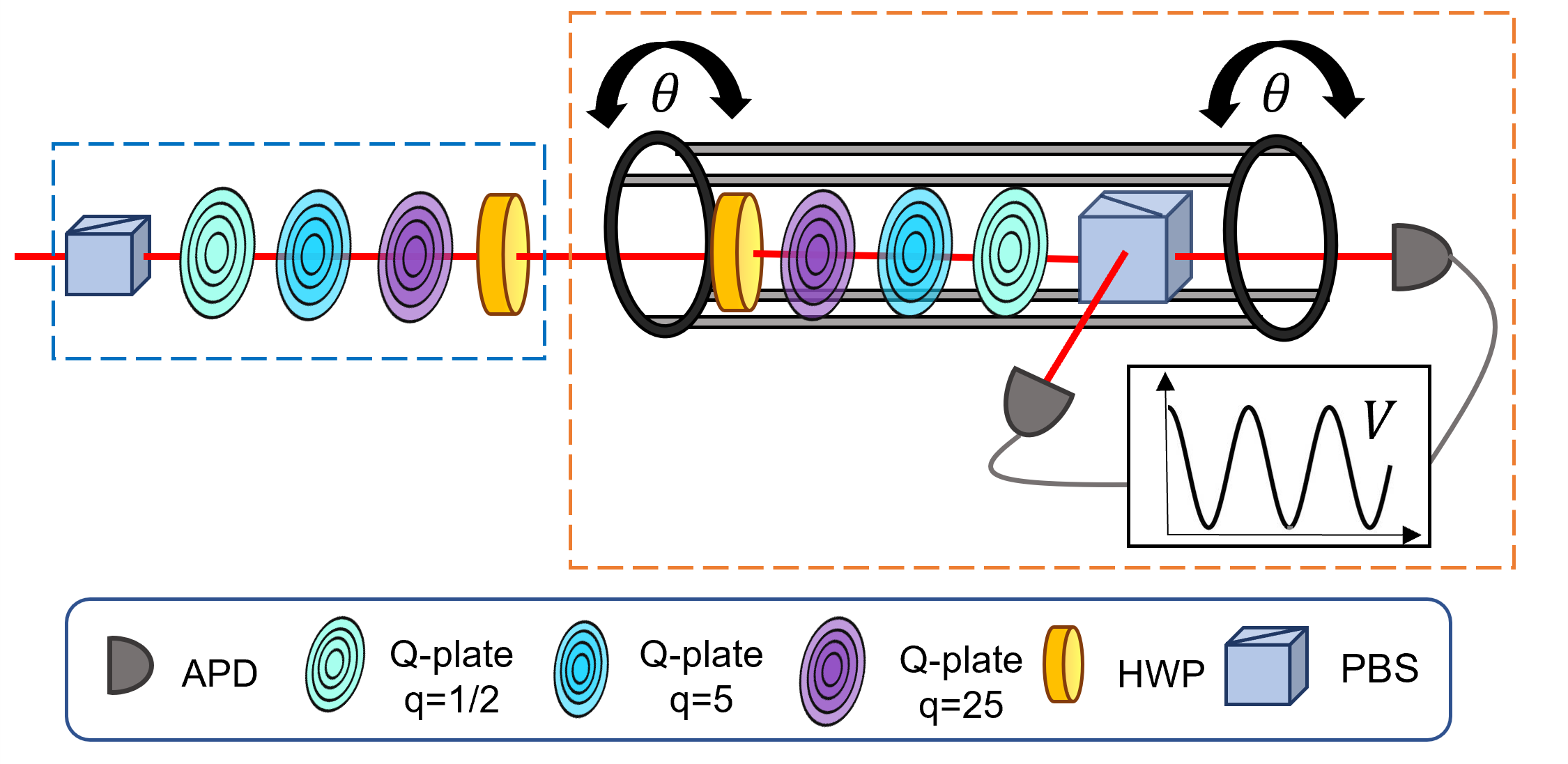
Figure 1: Sketch of the experimental setup. Single photons are sent through the apparatus consisting of a generation stage (blue rectangle) and a measurement stage (orange rectangle). The first is composed by a polarizing beam splitter (PBS) and three q-plates with different topological charges $q=1/2;5;25$, respectively, followed by a half-waveplate (HWP). The measurement stage is composed by the same elements of the preparation mounted in a compact and motorized cage which can be rotated by an angle $\theta$. After the final PBS, the photons are measured through avalanche photodiodes (APDs). The measurement HWP allows to set the polarization measurement basis.

Results and discussion - We start measuring the angle $\theta$ while treating the visibilities as nuisance unavoidable noises. To this end, we set the weight matrix $G$ in Eq. (1) to have $G_{11}=1$ as the only non-null entry. The data analysis is performed offline, and the raw data contains the outcome of the polarization measurement at the end of the receiving apparatus for many photons, for each rotation angle, q-plate, and polarization basis considered. We perform such measurements for $J=8$ different rotation angles in $[0,\pi)$, which corresponds to the periodicity interval of the system. On such collected measurement results we perform the Bayesian analysis setting the prior distributions on the visibilities as uniform in $[0,1]$, like the prior on the angle which is uniform in $[0,\pi)$. With the objective of minimizing the median error on the estimation of the rotation angle, the adaptive algorithm selects at each step the most appropriate quantum-like resource among the available ones. This is shown in the inset of Fig. 2a, where the estimation precision on the rotation angle is optimized by increasing gradually the momentum of the generated OAM states. The precision figure of merit achieved with such optimization strategy is reported in the main plot of Fig. 2a), where the experimental data are compared with the bound on the median in Eq (2), the Standard Quantum Limit (SQL) $1/N$ and the ultimate Heisenberg limit (HL) $\pi^{2}/N^{2}$ Górecki et al. (2020). The confidence interval for the median (plotted in light red) is evaluated with a bootstrap procedure for a $99\%$ confidence level. The experimental results show that the obtained error approaches the computed bound, which proves to be a valid reference even if non-tight. Notably, in such scenario, even if the visibility values are completely unknown, the implemented multiparameter protocol shows an enhanced estimation precision compared to the SQL for a large resources range, previously unexplored by multiparameter estimation experiments. Importantly, differently from Cimini et al. (2021) where the measurement strategy has been precalibrated according to the visibility values, here we show that it is still possible to obtain a non-negligible region showing sub-SQL performances treating the $4$ visibilities as nuisance parameters.

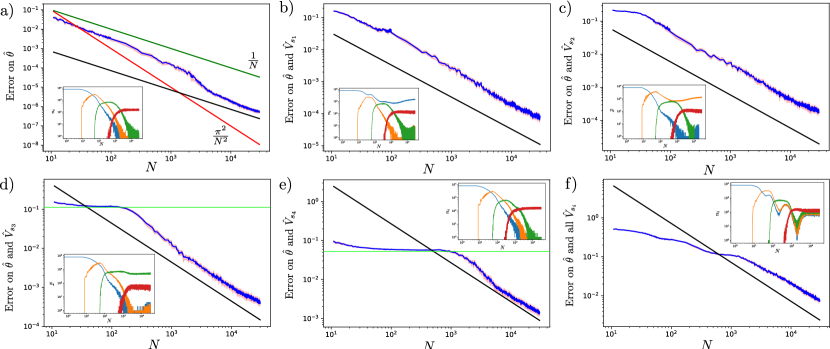
Figure 2: a) Plot of the median error for the phase only, with all the other parameters treated as nuisance parameters. The green line is the SQL$=1/N$, and the red one the HL$=\pi^{2}/N^{2}$. For all the plots the inserts are the number of uses of each q-plate in a batch of $10^{3}$ experiments for each of the $J=8$ angles as a function of the number of resources. In the inserts the blue lines correspond to photons with no OAM, the orange lines to $s=2$, the green lines to $s=11$ and the red ones to $s=51$. The intersection of these lines corresponds to the point at which the algorithm starts to suggest a q-plate with higher topological charge to perform the next experiment. Plots b), c), d), and e) refer respectively to the joint median error of the phase and each visibility $V_{s_{1}}$, $V_{s_{2}}$, $V_{s_{3}}$ and $V_{s_{4}}$. For each plot, all the other three visibilities are treated as nuisance parameters. Plot f) represents the precision for the phase and the joint estimation of all the four visibilities. The light green lines in d) and e) highlight the plateaus in the precision, that are discussed in the main text. The d) and e) plots show a scaling (slope of the black line) that in a limited region outperforms the classical ones. In all plots, the black line is the bound in Eq. (2) computed for the appropriate weight matrix $G$.

Then, we face the scenario where the visibilities are not treated anymore as nuisances but become themselves parameters which have to be estimated. This happens for instance if the user is interested in the full characterization of an interferometer, therefore needing an estimation of the noise levels. It is interesting to see how the optimization of the available resources changes in these new configurations. In particular, we shall focus on the scenario where one is interested in the estimation of the rotation angle and one of the visibilities (the $i_{0}$-th one), while the remaining ones are still treated as nuisance parameters. Under this assumption, the parameters of interest are the pair $(\theta,V_{s_{i_{0}}})$ with the median of the associated error computed by taking $G_{1,1}=G_{i_{0},i_{0}}=1$ in Eq. (1) as the only non-zero elements. As shown in Fig. 2, under this circumstance the Bayesian protocol, although switching to higher dimensional OAM states to decrease the error on the rotation angle, continues to use the q-plate related to the visibility chosen: this is necessary to obtain a good precision on the joint error. The results of the estimation of each of the four possible couples are reported in Fig. 2b, c, d and e. In particular, the plateaus in Fig. 2d and Fig. 2e appear since, for few resources, the q-plates corresponding to $s=11$ and $s=51$ are not significantly used. Therefore, the estimator of the corresponding visibilities remains the mean value of the uniform prior distribution in $[0,1]$, i.e. $0.5$, while the error on the phase decreases, thereby reaching a plateau determined by the value of the visibility $V_{i_{0}}$ itself. This changes only when the algorithm starts to use the high charge q-plates, and the error finally decreases. As a final observation, we notice that in the case where one focuses only on the phase $\theta$ there is still a pretty large region in which the slope of the estimation error with sub-SQL performances (specifically looking at Fig. 2a), this happens for values of $N$ between 2000 and 5000). Such behavior on the contrary is depressed when considering the estimation of the pairs $(\theta,V_{s_{i_{0}}})$ (only for $i_{0}=4$ there is a clear reminiscence of this, see Fig. 2e)). The reason for such behavior is related to the observation that the visibility is an inherently classical parameter and cannot benefit from the high angular momenta representing our quantum resources. We note that, the precision on the rotation angle maintains sub-SQL performances also in all the considered joint estimation scenarios. However, such enhanced performances are visible in the joint estimation errors of $(\theta,V_{4})$, see Fig. 2e) where the precision on the visibility parameter does not spoil the overall performances.

In summary, quantum sensing promises to be one of the first quantum technologies exploited to enhance tasks with respect to what is achievable with classical resources. Most of the realistic metrological problems involve more than one unknown parameter, which led to the birth of multiparameter quantum metrology. In this context, a fundamental problem is to optimally allocate the finite available resources, depending on which parameters are treated as nuisance noises and which are the parameters of interest. Furthermore, a crucial step is to reach quantum enhanced multiparameter estimations in a regime of large resources, where experimental demonstrations lack. In this work, we accomplished both these tasks by realizing a photonic setup with quantum elements (the q-plates) and considering different scenarios where the parameter of interest can be either the rotation angle only or the angle and the fringes visibility, treating the others as nuisance in the precision figure of merit. We experimentally showed that this approach is able to reach quantum-like performances in the estimation problems even when unknown nuisance noises are present, for a resources range $O(30,000)$. On one side, the obtained results have shown the possibility of extending the advantages of multiparameter quantum metrology in the large resource domain. On the other, the methodology here described can find application in large varieties of experimental platforms for quantum sensing, thus representing a tool for future generations of quantum sensors.