A Framework for Automated Correctness Checking of Biochemical Protocol Realizations on Digital Microfluidic Biochips

Abstract

Recent advances in digital microfluidic (DMF) technologies offer a promising platform for a wide variety of biochemical applications, such as DNA analysis, automated drug discovery, and toxicity monitoring. For on-chip implementation of complex bioassays, automated synthesis tools have been developed to meet the design challenges. Currently, the synthesis tools pass through a number of complex design steps to realize a given biochemical protocol on a target DMF architecture. Thus, design errors can arise during the synthesis steps. Before deploying a DMF biochip on a safety critical system, it is necessary to ensure that the desired biochemical protocol has been correctly implemented, i.e., the synthesized output (actuation sequences for the biochip) is free from any design or realization errors. We propose a symbolic constraint-based analysis framework for checking the correctness of a synthesized biochemical protocol with respect to the original design specification. The verification scheme based on this framework can detect several post-synthesis fluidic violations and realization errors in 2D-array based or pin-constrained biochips as well as in cyberphysical systems. It further generates diagnostic feedback for error localization. We present experimental results on the polymerase chain reaction (PCR) and in-vitro multiplexed bioassays to demonstrate the proposed verification approach.

I Introduction

Advances in digital microfluidic (DMF) technologies offer a promising platform for a variety of biochemical applications, ranging from massively parallel DNA analysis and computational drug discovery to toxicity monitoring and diagnosis [2]. The steady increase in complexity of biochemical protocols being implemented on DMF biochips has motivated the development of automated synthesis tools that take protocol descriptions as input and systematically synthesize efficient and optimized implementations. In this fast evolving landscape, ensuring that the synthesized biochips are functionally correct is crucial; an error in the functionality can not only delay product deployment, but also endanger human life in biomedical applications.

A synthesis tool [3] typically executes a series of transformations for implementing an input protocol description on a target architecture, as shown in Fig. 1. At first, the behavioral description of a bioassay (operations and dependence) is represented using a sequencing graph with appropriate design constraints (e.g., array area, completion time, resource constraints). This is followed by a sequence of synthesis steps, which include resource binding, scheduling, module placement, and droplet routing. Finally, a detailed layout of the DMF biochip (DMFB) along with the sequence of actuation steps are generated. Automated synthesis tools for DMF protocols today have reached a moderate level of sophistication and are ready to be deployed in practice [4, 5].

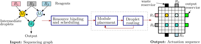
Figure 1: Synthesis flow of DMF biochips

As microfluidic technologies are poised to replace laboratory-based biochemical procedures, it is important to ensure the reliability and accuracy of a protocol realization. This becomes even more critical when biochips are deployed in life-critical or real-time systems. This necessitates the development of an automated procedure that can formally verify the synthesized implementation against the high-level design objectives, i.e., the input biochemical protocol to be realized and target-specific constraints. Post-synthesis verification is also important when a bioassay needs to be remapped onto an upgraded microfluidic platform. Verification in microelectrofluidic systems was classified as being either subjective or objective by Zhang et al. [6] but no mechanized procedure was proposed. A preliminary attempt towards design verification of flow-based microfluidic biochips has been reported by McDaniel et al. [7]. More recently, a one-pass symbolic correct-by-construction synthesis technique that satisfies fluidic and layout constraints has been proposed by Keszocze et al. [4].

In this paper, we propose an automated correctness checking framework for verifying post-synthesis realizations of biochemical protocols on a target DMF architecture. We adopt a symbolic constraint-based analysis method to achieve our objective. Given an actuation sequence generated by a synthesis tool for a given input sequencing graph to be realized on a DMF architecture, we adopt an incremental constraint-based analysis approach for checking if the actuation sequence indeed takes the assay through a safe state sequence free from fluidic constraint violations. We continue this checking procedure over the entire actuation sequence, as specified in the synthesized output and check for violations to ascertain that the generated actuation sequence is indeed safe for actual deployment. In addition, we reconstruct a sequencing graph as we traverse through the DMF states, and check it for operational correspondence with the original one to check if there are any timing or realization errors on the target architecture. Moreover, the verification tool notifies the user where the design rules are violated. This additional capability helps in error localization.

The objective of our framework is to detect synthesis tool as well as realization errors. Existing synthesis tools cycle through several optimization strategies and generally generate the solution in multiple passes. Given the sizes and complexities of today’s bioassays, it is therefore, quite an arduous task to debug the synthesis tool, just by observing the error manifestations at a user’s end. Note that in the past, similar efforts were made to formally check the correctness of circuit implementation in connection to logic synthesis tools [8]. However, such approaches did not fare well as they were not found to be practical for large systems. Also, an optimal one-pass synthesis tool that may work well for all protocols is hard to achieve, as evident from the scalability limitations witnessed in the one-pass approach [4]. Furthermore, many decisions such as the selection of the wash-droplet size may be made just before implementing the assay. Similarly, post-synthesis bugs may occur if the time needed for homogeneous mixing on the target platform is not properly characterized. Thus, rewriting a synthesis tool would not easily solve the problem of post-implementation correctness checking. Hence, we adopt a post-synthesis checking policy, where our objective is not to generate patches for synthesis tools, but to detect the errors arising out of imprecise synthesis strategies and the choice of target architecture. Our proposal can be thought of as the first step towards a verification methodology in the context of microfluidic computation, and we expect that the generality of our verification techniques will eventually allow us to apply them not only to DMF-based assay implementations, but to a wider class of microfluidic paradigms. We demonstrate that in addition to general-purpose biochip architectures, our method is applicable to pin-constrained chips and cyberphysical systems. We also present an extensive case study on several real-life bioassay descriptions.

The rest of the article is organized as follows. Section II summarizes the various constraints needed for verifying design errors for a general-purpose DMFB. Section III discusses the correctness issues related to pin-constrained DMFBs. Section IV describes the design constraint analysis and the procedure for conformance checking between the input sequencing graph and the synthesized graph. The architectural description of the verification engine and a software visualization tool SimBioSys, are described in Section V. Experimental results for two real life biochemical assays are presented in Section VI. The correctness checking procedure for fault-tolerant assays implemented in a cyberphysical scenario is described in Section VII. Finally, Section VIII concludes the article and highlights directions for future work.

II Verification of general-purpose fully reconfigurable DMF Biochips

In this section, we describe several facets of the verification problem that may arise in the context of fully reconfigurable DMFBs. We assume that a DMFB platform is capable of performing basic fluidic operations such as dispensing a droplet from a reservoir, moving a droplet, and mixing/splitting of two droplets.

The dilution of a sample and the mixing of reagents are basic steps in a biochemical protocol [9]. The concentration factor $(CF)$ of a sample is defined as the ratio of initial volume of the raw sample to the final volume of the prepared mixture. Thus, $0\leq CF\leq 1$.

In this work, we assume the ($1:1$) mixing model, i.e., every mix-split cycle consists of a mix operation between two unit-volume fluid droplets followed by a balanced split operation of the mixed fluid. Hence, for the sake of convenience, the $CF$ of a reagent in a target droplet is expressed as an $n$-bit binary fraction (by rounding it off beyond the $n$-th bit), when an accuracy level of $n$ (i.e., maximum allowable error in $CF$ is $\frac{1}{2^{n+1}}$) is desired in $CF$. In other words, the $CF$ of a target droplet can be expressed as $\frac{x}{2^{n}}$, where $x\in\mathbb{Z}^{+}$, $0\leq x\leq 2^{n}-1$. Note that, the $CF$ of a raw sample and a buffer can be represented by $\frac{2^{n}}{2^{n}}$ and $\frac{0}{2^{n}}$ respectively.

The following example demonstrates the various challenges that may arise in a protocol-verification problem.

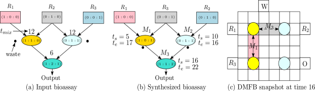
Figure 2: Behavioral description of (a) input and (b) synthesized bioassay with an (c) error instance

Example 1.

Fig. 2 shows the behavioral description of an input bioassay and the corresponding one extracted from the realization generated by the synthesis tool. The input specification is given as a sequencing graph ($SG$) [10], which is commonly used for describing dependencies between assay operations (e.g., dispensing, mixing). Fig. 2(a) represents the input $SG$ for preparing a mixture of three input reagents $(R_{1},R_{2},R_{3})$ in a ratio $(1:2:1)$, where $t_{mix}$ represents the mixing time required for homogeneous mixing. Our verification tool extracts a directed acyclic graph (DAG) representing the realized bioassay. Fig. 2(b) shows the $SG$ of the synthesized bioassay, where $t_{s}$ and $t_{e}$ denote the mixing start and end times respectively. Unfortunately, the actuation sequences generated by the synthesis tool incorrectly interchanges $R_{2}$ and $R_{3}$. As a result, the output droplets produced in Fig. 2(b) have a different ratio of input reagents $(1:1:2)$, i.e., the input bioassay is realized incorrectly. This is an instance of the error $e_{7}$ in Table LABEL:tab:design-error. From Fig. 2(b), it can be observed that the mixing time of $R_{2}$ and $R_{3}$ is 6, but the input bioassay specifies that $R_{2}$ and $R_{3}$ should be mixed for 12 time units. Hence, an inhomogeneous mixing might have taken place $(e_{6})$, resulting in a violation.

A different design error can be observed at the output node in Fig. 2(b), where mixing starts at 16. In the snapshot of the DMFB at time 16 (Fig.  2(c)), mixer $M_{3}$ is instantiated by receiving a droplet from mixer $M_{1}$. However, the latter completes the mix-operation at time instant 17 (Fig.  2(b)), leading to an incorrect realization of the bioassay $(e_{4})$. $\blacksquare$

[ caption = Possible design errors and their consequences, label = tab:design-error, pos = !t, width = 0.48framesep=0pt, framerule = 1pt, doinside = ]p1ptp123ptX Design error Consequence $e_{1}$ Violation of static fluidic constraints (FC) Unintentional mix of droplets $e_{2}$ Violation of dynamic FC Unintentional mix of droplets $e_{3}$ Dispensing to/from wrong reservoir Incorrect fluidic operation $e_{4}$ Move droplets to/from active mixers; late arrival or early exit Incorrect fluidic operation $e_{5}$ Instantiate mixer with incorrect number of droplets Droplet routing error or Incorrect fluidic operation $e_{6}$ Mixing droplets for lesser amount of time than specified Inhomogeneous mixing $e_{7}$ Wrong mix-split operations Incorrect realization of input assay

There can be several other design realization errors that may creep into the design process. Table LABEL:tab:design-error shows some possible design realization errors, which may lead to undesirable violations, including those described in Example 1. The list of errors have been compiled based on those reported in practice [11, 12, 13, 14]. We have also witnessed similar errors while using the synthesis tools on several common protocols, e.g., PCR.

We have adopted a symbolic constraint-based incremental analysis framework for ensuring post-synthesis correctness of the DMF protocol realizations. The constraints may either be fluidic (both static and dynamic), as imposed by DMF design guidelines [10], or imposed by the target architecture on which the input protocol is to be realized. In doing so, for the sake of uniformity and portability across synthesis tools, we work on a simple intermediate instruction-set architecture language for representing and manipulating actuation sequences (obtained by a simple transformation on the actuation sequences produced by a standard synthesis tool), in which the synthesized output obtained from a DMF synthesizer can be concisely described. Our method has two main steps. In the first step, we perform an incremental analysis of the fluidic operation actuation sequences generated by the synthesis tool and look for DMFB realization errors. If any violation is found, the potential cause of violation, i.e., which fluidic operation causes violation of a design rule, is reported immediately. At the end of the design verification process, if no errors are reported, the synthesized $SG$ is generated. In the second step, the synthesized sequencing graph is checked for conformance with the input protocol graph (Section IV). This is done by a variant of the labeled DAG traversal algorithm. If the synthesized $SG$ does not correctly realize the input specification, potential violations are reported for diagnostics.

II-A Modeling formalisms

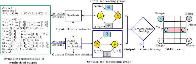
Figure 3: Verification engine

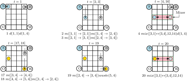
Figure 4: Execution of synthesized instructions

In this subsection, we address the correctness checking problem in the context of fully reconfigurable DMFBs. The overall architecture of our verification engine is shown in Fig. 3. It internally translates the synthesized output into an intermediate format and incrementally looks for constraint violations. If no violations are observed, it outputs a transformed synthesized $SG$ that is checked for conformance against the original input. Formally, the correctness checking problem can be formulated as below:

• Inputs:

  • Behavioral description of the protocol;

  • The output of a synthesis tool (actuation sequences to be executed on the target DMF biochip);

  • Parameters of the target DMF architecture:

    • Biochip dimensions.

    • Reservoirs and their locations.

  • Design constraints

    • Fluidic constraints (static and dynamic).

    • Maximum bioassay completion time $(T_{max})$.

• Output:

  • Yes, if all design rules are met and the input protocol is correctly realized.

  • No, with a counterexample showing possible causes of violation.

Behavioral description of the protocol

The input behavioral description of the bioassay is represented as a $SG$, defined as follows. A $SG$ is a directed acyclic graph $G(V,E)$ with vertex set $V=\{v_{i}:i=0,1,\ldots,k\}$ and an edge set $E=\{(v_{i},v_{j})$: $i,j\in\{0,1,\ldots,k\}\}$. Each vertex corresponds to an assay operation (e.g., dispensing, mixing), while the edges capture the precedence relationships between the operations. Note that for compact representation, multiple dispense operations of the same reagent are merged into a single node (drawn as square) in the $SG$. A vertex $v_{i}$ can optionally be labeled with a number $t(v_{i})$, which denotes the time taken for the operation used at $v_{i}$.

Example 2.

The input $SG$ in Fig. 3 shows the dilution graph generating a target dilution having concentration factor $\frac{8}{32}$ using only sample $(\frac{32}{32})$ and buffer $(\frac{0}{32})$ using twoWayMix [9] method. It may be noted that each mixing operation takes 12 time units for homogeneous mixing. $\blacksquare$

We introduce a compact symbolic encoding of the actuation sequence generated by a synthesis tool in an intermediate language, which is expressive enough to capture all commonly used fluidic operations. The semantics of the instruction set is described in Table LABEL:tab:instructions. The instruction set considered in Table LABEL:tab:instructions is designed to capture the most common operation types, as witnessed in common bioassay protocols. For more enhanced protocol instructions, this instruction set can be augmented with additional constructs. In Section VII, we have shown an example of an error-tolerant synthesis strategy, which is being studied today in the context of cyber-physical systems. We have added two new features (optical detection and conditionals) to enhance our repertoire of instructions. The proposed correctness checking method is flexible enough to accommodate such additional instructions as required.

[ caption = Fluidic instructions and their interpretations, label = tab:instructions, pos = !h, width = 0.48framesep=0pt, framerule = 1pt, doinside = ]p70ptX adjacent left, right, top and bottom cells Encoding Architectural description $dim(r,c)$ Dimension of the biochip, $r$ rows and $c$ columns, each cell is addressed as $(i,j)$, where $1\leq i\leq r$ and$1\leq j\leq c$ $R(r,c,Name)$ Reagent reservoir from which droplets can be dispensed. Droplet dispensed from reagent reservoir at $(r,c)$ and $Name$ denotes reagent’s name $O(r,c)$/$W(r,c)$ Output/waste reservoir, where $(r,c)$ denotes the cell from which a droplet can be sent to output/waste reservoir Instruction Fluidic operational description $d$($r,c$) Dispense droplet from reservoir at location ($r,c$) $m$([$r_{1},c_{1}$]$\to$[$r_{2},c_{2}$]) Transport droplet at location ($r_{1},c_{1}$) to ($r_{2},c_{2}$). It moves a droplet at ($r_{1},c_{1}$) to one of its 4-neighbors($N_{4}(r_{1},c_{1})$) i.e., $(r_{2},c_{2})\in N_{4}(r_{1},c_{1})$$mix$([$r_{1},c_{1}$]$\leftrightarrow$[$r_{2},c_{2}$],           $t_{mix},mtype$) Mix two droplets at ($r_{1},c_{1}$) and ($r_{2},c_{2}$) for $t_{mix}$ time steps. Initial locations are determined by the type of mixer $(mtype)$. At the end of the mixing operation, two droplets are generated and stored at locations ($r_{1},c_{1}$) and ($r_{2},c_{2}$) respectively $waste(r,c)$/$output(r,c)$ Dispense droplet at ($r,c$) to its adjacent waste/output reservoir $end$ End of bioassay Encoding Bioassay parameter $accuracy$ $n$ Given $N$ input reagents, each concentration is represented as $C=\frac{a_{1}R_{1}+a_{2}R_{2}+\ldots+a_{N}R_{N}}{2^{n}}$, where $\sum_{k=1}^{N}a_{k}=2^{n}$ and $a_{k}$ is a positive integer and $R_{k}$ is an input reagent for $k=1,2,\ldots,N$

Fig. 3 shows an example encoding of a synthesized actuation sequence. The first three lines define the dimension of the biochip, desired accuracy of concentration, and reservoir locations respectively. Each instruction line contains one or more symbolic fluidic instruction, separated by space. The instructions occurring on the same line are concurrent, i.e., they are executed simultaneously. The numeric label prefixing each instruction line stands for the start time of the instructions at that line. We assume that every primitive instruction, except ‘$mix([r_{1},c_{1}]\leftrightarrow[r_{2},c_{2}],t_{mix},mtype)$’, takes unit time.

Example 3.

Interpretations of the different instructions are illustrated in Fig. 4, where $S,B,W$ and $O$ denote the sample dispenser, buffer dispensers, waste reservoir and output reservoir, respectively. The first three lines of the synthesized output in Fig. 3 describe the architectural description of the DMF platform on which the actuation sequences will execute. In this case, the biochip has 5 rows and 4 columns, i.e., it has 20 cells $(dim\>5\,4)$. Two reagent reservoirs, namely sample (S) and buffer (B) dispense droplets to $(1,1)$ and $(1,4)$ locations, respectively. Analogously, one waste and one output reservoir dispense droplets from $(5,4)$ and $(5,1)$ respectively. These dispense operations are denoted as $R(1,1,S)\>R(1,4,B)\>O(5,1)\>W(5,4)$. The accuracy level is set to 5, i.e., each concentration factor is approximated as $C=\frac{a_{1}S+a_{2}B}{2^{5}}$, where $a_{1}+a_{2}=2^{5}$.

We now describe the execution semantics of the symbolic fluidic operations on the DMFB platform discussed in the previous paragraph. Some snapshots over different time steps are shown in Fig. 4, where instructions are shown beneath the figure and the time interval is shown on top of the figure. At $t=1$, two droplets are dispensed from sample (S) and buffer (B) reservoirs. At $t=2$ and $t=3$, both the droplets are simultaneously moved one cell downward. At $t=4$, a buffer droplet is dispensed to location $(1,4)$ and a $1\times 4$ mixer is instantiated, which remains active for the next 12 time steps. At $t=17$, mixing/splitting is completed and two droplets are present at locations $(3,1)$ and $(3,4)$. The droplet at $(3,4)$ is then moved downward. In the next time step, i.e., $t=18$, droplets at $(1,4)$ and $(4,4)$ are simultaneously moved to $(2,4)$ and $(5,4)$ locations respectively. At $t=19$, the droplet at $(2,4)$ is moved to $(3,4)$ and the waste droplet at $(5,4)$ is dispatched to the waste reservoir. At a subsequent time $t=20$, a new mixing operation is performed between the droplets at $(3,1)$ and $(3,4)$ using a $1\times 4$ mixer which remains active during the subsequent 12 time steps. The remaining instructions of the synthesized bioassay (Fig. 3) are executed as specified, and have similar execution semantics. $\blacksquare$

Parameters of the target DMF architecture

In order to perform automated correctness checking of the synthesized bioassay, it is essential to know the architectural description of the target DMF platform where the synthesized bioassay will be executed such as its dimensions, the reservoir locations, and their contents (reagent, output, waste).

Design constraints

Automated synthesis tools generate actuation sequences that have to satisfy some design constraints. As an example, both static and dynamic fluidic constraints  [10] (Section II) need to be satisfied for unintentional mixing of droplets. Another example of a design constraint is the maximum bioassay completion time $(T_{max})$, which dictates that the synthesized bioassay should be completed within a specified time limit. In order to ensure correct realization of the input protocol, there are several other design constraints that need to be satisfied.

II-B Constraint modeling

We now describe the overall constraint modeling and verification scheme. We create Boolean formulas for verifying each of the fluidic instructions. Logical operators are used for negation $(\neg)$, and $(\wedge)$, or $(\vee)$ of Boolean variables. Let us consider a two-dimensional biochip of size $r\times c$, where $r$ and $c$ denote the number of rows and columns of the target DMFB, respectively.

We define an indicator Boolean variable $x_{i,j}^{t}$ denoting the state of a biochip cell at location $(i,j)$, where $1\leq i\leq r$, $1\leq j\leq c$ and $t$ is the time index. We encode a biochip description symbolically at time instant $t$ using $B_{r\times c}^{t}$, which is the conjunction of all state variables at time $t$. We define a few Boolean functions and auxiliary tables that represent different constraints and description of on-chip reservoirs, active mixers in the layout.

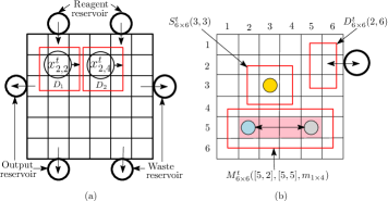
Figure 5: (a) Boolean variables for biochip description and fluidic constraints. (b) Notation for design constraints.

Modeling Fluidic constraints

During droplet routing, a minimum spacing between droplets must be maintained to prevent accidental mixing, unless droplet merging is desired. Such fluidic constraints (FC) [10] are usually classified as static or dynamic, depending on the type of operation it relates to.

Definition 1.

[Static Fluidic constraint:] If a droplet is on cell $(i,j)$ at time $t$, then no other droplet can reside in the 8-neighboring cells of $(i,j)$ at time $t$, denoted as $N_{8}(i,j)$. $\blacksquare$

For example, in Fig. 5(a), the static fluidic constraint for the droplet on cell $(2,2)$ at $t$ is shown as a surrounded box of cells which should not be used by any other droplet at $t$.

Static fluidic constraint for a droplet on cell $(i,j)$ can be expressed as:

$$S_{r\times c}^{t}(i,j)=x_{i,j}^{t} \wedge_{(i_{1},j_{1})\in N_{8}(i,j)}\neg x_{i_{1},j_{1}}^{t}$$ (1)

$$\qquad{}\text{where }1\leq i_{1}\leq r,1\leq j_{1}\leq c$$

For example, in Fig. 5(b), the static fluidic constraint for the droplet at $(3,3)$ at $t$ will be modeled as $S_{6\times 6}^{t}(3,3)=\neg x_{2,2}^{t}\wedge\neg x_{2,3}^{t}\wedge\neg x_{2,4}^{t}\wedge\neg x_{3,2}^{t}\wedge x_{3,3}^{t}\wedge\neg x_{3,4}^{t}\wedge\neg x_{4,2}^{t}\wedge\neg x_{4,3}^{t}\wedge\neg x_{4,4}^{t}$

Definition 2.

[Dynamic Fluidic constraint:] Every movement operation at an instant $t+1$ must honor the 8-neighborhood isolation of all other droplets at time $t$. $\blacksquare$

In other words, the activated cell for droplet $D_{i}$ cannot be adjacent to $D_{j}$, otherwise, there is more than one activated neighboring cell for $D_{j}$, which may lead to errant fluidic operations. Consider Fig. 5(a) with two droplets $D_{1}$ and $D_{2}$ at locations $(2,2)$ and $(2,4)$ respectively. If both $D_{1}$ and $D_{2}$ want to move one cell right at $t+1$, two neighboring cells of $D_{2}$ are actuated simultaneously. Although the static fluidic constraint is satisfied, this situation may still lead to unintentional mixing of droplets at location $(2,3)$. As a result, $D_{1}$ moves rapidly to $(2,3)$ while the droplet $D_{2}$ moves slowly towards $(2,5)$.

Modeling of dynamic fluidic constraints is non-trivial since it depends on the exact type of the movement operation. We describe below two other types of constraints that relate to dispensing and mixing.

Definition 3.

[Dispensing constraint:] Before dispensing a droplet at $(i,j)$, no droplet should be present either at $(i,j)$ or in its 8-neighborhood. $\blacksquare$

This constraint can be expressed as:

$$D_{r\times c}^{t}(i,j)=\neg x_{i,j}^{t} \wedge_{(i_{1},j_{1})\in N_{8}(i,j)}\neg x_{i_{1},j_{1}}^{t}$$ (2)

$$\qquad{}\text{where }1\leq i_{1}\leq r,1\leq j_{1}\leq c$$

In Fig. 5(b), $D_{r\times c}^{t}(2,6)$ denotes the constraint that needs to be satisfied before dispensing a droplet from a reservoir to cell $(2,6)$ at time $t$. Hence, $D_{r\times c}^{t}(2,6)=\wedge_{(1\leq i\leq 3)}\neg x_{i,5}^{t}\wedge\neg x_{i,6}^{t}$.

Definition 4.

[Mixer constraint:] No droplet should be present in the adjacent cells of active mixers. $\blacksquare$

This constraint is needed to prevent unintentional droplet mixing. The expression for this constraint varies with the type of the mixer ($mtype$). Intuitively, this captures the restriction that the droplets to be mixed should be available at the mixer-input specified locations, while also honoring the neighborhood constraint in the adjacency of the mixing locations.

Let $M_{r\times c}^{t}([r_{1},c_{1}],[r_{2},c_{2}],mtype)$ denote the mixer constraint for an active mixer. Note that for each type of mixer, it takes two input droplets at location $(r_{1},c_{1})$ and $(r_{2},c_{2})$ and produces two output droplets at the same locations. For simplicity, we have considered only $1\times 4$ ($mtype=14$) and $4\times 1$ ($mtype=41$) mixers.

Example 4.

For a $1\times 4$ linear array, i.e., $mtype=14$, the mixer constraint can be expressed as:

$$M_{r\times c}^{t}([r_{1},c_{1}],[r_{2},c_{2}],14)=S_{r\times c}^{t}(r_{1},c_{1})\wedge S_{r\times c}^{t}(r_{2},c_{2})$$ (3)

In Fig. 5(b), the mixer constraint $M_{6\times 6}^{t}([5,2],[5,5],14)$ for a $1\times 4$ mixer with two droplets at locations $(5,2)$ and $(5,5)$ can be expressed as $\wedge_{(1\leq j\leq 6)}\neg x_{4,j}^{t}\wedge\neg x_{5,1}^{t}\wedge x_{5,2}^{t}\wedge\neg x_{5,3}^{t}\wedge\neg x_{5,4}^{t}\wedge x_{5,5}^{t}\wedge\neg x_{5,6}^{t}\wedge_{(1\leq j\leq 6)}\neg x_{6,j}^{t}$. $\blacksquare$

In the special case of a $1\times 4$ or $4\times 1$ mixer, where the two input/output droplets are in the leftmost and rightmost cells, the mixer constraint can be described by the conjunction of the static fluidic constraints of the two droplet locations. However, for other types of mixers, the constraint in Eqn. 3 needs to be suitably modified for preventing any interference with other droplets.

A table $T_{reservoir}$ stores the on-chip reservoir descriptions as $(i,j,rtype)$, where $(i,j)$ is the dispenser location and $rtype$ is the reservoir type (reagent, output, waste). For correctness checking of each dispense operation, $T_{reservoir}$ is accessed for verifying the correct dispense location. Similarly, a table $T_{mixer}$ maintains the descriptions of active mixers in the form of $([r_{1},c_{1}],[r_{2},c_{2}],t_{s},t_{e},mtype)$, where $[r_{1},c_{1}],[r_{2},c_{2}]$ are the locations of the two droplets to be mixed with an $mtype$ mixer and $t_{s},t_{e}$ are start and end times of a mixing operation. In our incremental correctness checking procedure, we change the DMF state depending on the current state and the set of fluidic operations to be executed at the subsequent time instants. As mixer instantiation spans over multiple time steps, we need to store active mixers in $T_{mixer}$ so that the necessary updating of DMF states can be made on completion of an active mixing at a particular time step. Table LABEL:tab:constraints summarizes the notations we are using.

[ caption = Notation, label = tab:constraints, pos = !h, width = 0.48framesep=0pt, framerule = 1pt, doinside = ]p25ptX Boolean function Constraint $B_{r\times c}^{t}$ Symbolic description of biochip of size $r\times c$ at time $t$.$S_{r\times c}^{t}(i,j)$ Defined on state variables at time $t$, that represents the static FC of a droplet at $(i,j)$ in a biochip of size $r\times c$$D_{r\times c}^{t}(i,j)$ Represents FCs that must be satisfied before dispensing droplet at $(i,j)$$M_{r\times c}^{t}([r_{1},c_{1}],$$[r_{2},c_{2}],mtype)$ Represents static FC for an active mixer of type $mtype$ at time $t$ Table Description $T_{mixer}$ Maintains active mixers. Each entry is in the form of $([r_{1},c_{1}],[r_{2},c_{2}],t_{s},t_{e},mtype)$, where $[r_{1},c_{1}],[r_{2},c_{2}]$ are the positions of the two droplets to be mixed with a $mtype$ mixer and $t_{s},t_{e}$ are start and end times of the mixing operation$T_{reservoir}$ Stores the description of on-chip reservoir. Each entry is of the form $(i,j,rtype)$, where $(i,j)$ is the dispense location and $rtype$ is the reservoir type (reagent, output, waste)

Modeling the initial configuration

The first three lines of the synthesized output describe the architectural description of the DMF platform on which the input bioassay is to be executed. From the architectural description of the synthesized output, on-chip reservoir descriptions are stored in $T_{resrevoir}$ along with its type (input/output/waste reservoir). Moreover, the mixer table is initialized, i.e., $T_{mixer}=\phi$, as the biochip has no droplets to be mixed initially $(t=0)$. Hence, the symbolic representation of the biochip at $t=0$ is

$$B_{r\times c}^{0}=\wedge_{(1\leq i\leq r,1\leq j\leq c)}\neg x_{i,j}^{0}$$ (4)

In subsequent time steps, some fluidic operations are executed, which lead to a change in the description. In general, we have $B_{r\times c}^{t}$ and some fluidic operation executed at $t+1$. We need to verify whether these operations are valid on the current configuration ($B_{r\times c}^{t}$) and change the biochip to an allowable configuration at $t+1$, i.e., $B_{r\times c}^{t+1}$ is valid at $t+1$.

Modeling of fluidic operations

We now illustrate the modeling of each fluidic operation executed at $t+1$ on $B_{r\times c}^{t}$. In the illustrative examples, we only list the true variables explicitly in the symbolic representation of the biochip. All other negated variables are assumed to be implicitly present.

Dispense of a reagent droplet – $d(i,j)$: Before dispensing a droplet from a reagent reservoir to a cell $(i,j)$, one has to ensure that the droplet is being dispensed from a reagent reservoir. This can be checked by a look-up on $T_{reservoir}$. Also, after dispensing the droplet at $(i,j)$, no fluidic violation should occur. This can be verified using the expression:

$$E_{d}^{FC}=D_{r\times c}^{t}(i,j)\wedge B_{r\times c}^{t}$$ (5)

If $E_{d}^{FC}$ is $true$, the fluidic constraints are satisfied. The truth value checking procedure has been elaborated in Section V. It can be easily verified that $E_{d}^{FC}$ is $true$ only when there is no droplet present at the location $(i,j)$ and its adjacent locations at time $t$. It is important to ensure that only one droplet is dispensed on a particular location at $t+1$. This can be done in the following way.

After dispensing a droplet to a valid location at a time step $t+1$, it is important to check that no droplet is dispensed on the same location at the same time step. For ensuring this, we need to modify $B_{r\times c}^{t}$ to reflect that the droplet is on $(i,j)$ at $t$. In doing so, we need to update $B_{r\times c}^{t}$ with $x_{i,j}^{t}$. After this modification, if we want to dispense another droplet at $(i,j)$, it violates the fluidic constraints since the updated $B_{r\times c}^{t}$ shows a droplet present at $(i,j)$ at time $t$. Finally, $B_{r\times c}^{t+1}$ is updated with $x_{i,j}^{t+1}$ for representing the dispensed droplet on the biochip at $t+1$. We explain this on the following example.

Figure 6: Verifying the dispense operation

Example 5.

In Fig. 6, the biochip description at $t$ is $B_{5\times 4}^{t}=x_{3,3}^{t}\wedge x_{4,1}^{t}\wedge x_{5,4}^{t}$ (negated variables are implicit) and at $t+1$, a dispense instruction $d(1,1)$ is to be executed. $E_{d}^{FC}$ is $true$, i.e, fluidic constraints are preserved. We must update $B_{5\times 4}^{t}$ with $x_{1,1}^{t}$ to prevent multiple dispense on the same location $(1,1)$ at $t+1$. Hence, $B_{5\times 4}^{t}$ becomes $x_{1,1}^{t}\wedge x_{3,3}^{t}\wedge x_{4,1}^{t}\wedge x_{5,4}^{t}$ i.e., $\neg x_{1,1}^{t}$ is removed and $x_{1,1}^{t}$ is added. Note that after updating $B_{5\times 4}^{t}$, any operation trying to dispense a droplet on the same location is prohibited. Now, consider a case where a droplet exists on $(2,2)$ at $t$. $B_{5\times 4}^{t}$ will be $x_{2,2}^{t}\wedge x_{3,3}^{t}\wedge x_{4,1}^{t}\wedge x_{5,4}^{t}$ and $D_{5\times 4}^{t}(1,1)$ is $\neg x_{1,1}^{t}\wedge\neg x_{1,2}^{t}\wedge\neg x_{2,1}^{t}\wedge\neg x_{2,2}^{t}$. Note that $B_{5\times 4}^{t}\wedge D_{5\times 4}^{t}(1,1)$ is $false$ and therefore, generates a conflict. Hence, this dispense is not safe. $B_{5\times 4}^{t+1}$ becomes $x_{1,1}^{t+1}\wedge x_{3,3}^{t+1}\wedge x_{4,1}^{t+1}\wedge x_{5,4}^{t+1}$. $\blacksquare$

Dispensing a droplet to a waste reservoir – $waste(i,j)$: This is similar to d($i,j$), except that waste reservoirs are considered instead of reagent reservoirs. This can be expressed as:

$$E_{waste}^{FC}=x_{i,j}^{t}\wedge B_{r\times c}^{t}$$ (6)

$E_{waste}^{FC}$ is $true$ if a droplet is present on $(i,j)$ before dispensing. As earlier, in this case as well, we must update $B_{r\times c}^{t}$ with $\neg x_{i,j}^{t}$ to prevent multiple dispense to the waste reservoir from the same location $(i,j)$ at $t+1$. $B_{r\times c}^{t+1}$ is updated with $\neg x_{i,j}^{t+1}$ to capture the fact that the cell is now available, since the droplet occupying the cell has been dispensed to a waste reservoir.

Dispensing a droplet to an output reservoir – $output(i,j)$: The formulation for this is similar to waste($i,j$), except that output reservoirs are considered. This can be expressed as:

$$E_{output}^{FC}=x_{i,j}^{t}\wedge B_{r\times c}^{t}$$ (7)

As earlier, $E_{output}^{FC}$ must be $true$ before dispensing. Analogously, $B_{r\times c}^{t}$ and $B_{r\times c}^{t+1}$ are updated with $\neg x_{i,j}^{t}$ and $\neg x_{i,j}^{t+1}$ respectively.

Transportation of a droplet – $m([r_{1},c_{1}]\to[r_{2},c_{2}])$: The move instruction $m$ transports a droplet from a valid DMFB location $(r_{1},c_{1})$ to one of its four neighbors $(r_{2},c_{2})$ i.e., $(r_{2},c_{2})\in N_{4}(r_{1},c_{1})$. The static and dynamic fluidic constraints need to be satisfied in the move operation. The fluidic constraint for this operation can be expressed as:

$$E_{m}^{FC}=x_{r_{1},c_{1}}^{t}\wedge E\wedge B_{r\times c}^{t}$$ (8)

The expression $E$ is used for checking dynamic fluidic constraints and is defined as follows:

$$\scriptsize E=\begin{cases}\neg x_{r_{2}-1,c_{2}+1}^{t}\wedge\neg x_{r_{2},c_{2}+1}^{t}\wedge\neg x_{r_{2}+1,c_{2}+1}^{t}&\mbox{for right ($\rightarrow$) move }\\ \neg x_{r_{2}-1,c_{2}-1}^{t}\wedge\neg x_{r_{2},c_{2}-1}^{t}\wedge\neg x_{r_{2}+1,c_{2}-1}^{t}&\mbox{for left ($\leftarrow$) move }\\ \neg x_{r_{2}+1,c_{2}-1}^{t}\wedge\neg x_{r_{2}+1,c_{2}}^{t}\wedge\neg x_{r_{2}+1,c_{2}+1}^{t}&\mbox{for bottom ($\downarrow$) move }\\ \neg x_{r_{2}-1,c_{2}-1}^{t}\wedge\neg x_{r_{2}-1,c_{2}}^{t}\wedge\neg x_{r_{2}-1,c_{2}+1}^{t}&\mbox{for top ($\uparrow$) move }\\ \end{cases}$$

Note that $x_{r_{1},c_{1}}^{t}\wedge B_{r\times c}^{t}$ is $true$ when a droplet is present on $(r_{1},c_{1})$ at time $t$. Analogously, the dynamic fluidic constraint is satisfied if $E\wedge B_{r\times c}^{t}$ is $true$ i.e., no droplet is present at the neighboring locations of the move destination. $B_{r\times c}^{t+1}$ is updated with $\neg x_{r_{1},c_{1}}^{t+1}\wedge x_{r_{2},c_{2}}^{t+1}$ for reflecting the effect of the move operation at $t+1$. It may be noted that the neighborhood constraint for $(r_{2},c_{2})$ is already ensured partially by the fact that the present configuration with a droplet at $(r_{1},c_{1})$ at time $t$ satisfies all static fluidic constraints.

Figure 7: Verifying the move operation.

Example 6.

Consider the example shown in Fig. 7 where $B_{5\times 4}^{t}=x_{3,3}^{t}\wedge x_{4,1}^{t}\wedge x_{5,4}^{t}$. At $t+1$, a move instruction $m([3,3]\rightarrow[2,3])$ is executed. Note that the move destination is one of the 4-neighbors of $(3,3)$. $E_{m}^{FC}=x_{3,3}^{t}\wedge(\neg x_{1,2}^{t}\wedge\neg x_{1,3}^{t}\wedge\neg x_{1,4}^{t})\wedge(x_{3,3}^{t}\wedge x_{4,1}^{t}\wedge x_{5,4}^{t})$ is $true$. So, a droplet is present on $(3,3)$ at $t$ and when it is moved to $(2,3)$ no fluidic constraints are violated.

Consider the case where $m([3,3]\rightarrow[3,2])$ is executed at $t+1$ instead of $m([3,3]\rightarrow[2,3])$. Note that $E_{m}^{FC}=x_{3,3}^{t}\wedge(\neg x_{2,1}^{t}\wedge\neg x_{3,1}^{t}\wedge\neg x_{4,1}^{t})\wedge(x_{3,3}^{t}\wedge x_{4,1}^{t}\wedge x_{5,4}^{t})$ is $false$ because it conflicts on variable $x_{4,1}^{t}$. Hence, the instruction $m([3,3]\rightarrow[3,2])$ violates the fluidic constraint. $\blacksquare$

Mixing operation – $mix([r_{1},c_{1}]\leftrightarrow[r_{2},c_{2}],t_{mix},mtype$): The expression for a mixer depends on the mixer type $(mtype)$. Depending on the type, the verification of the mixer instantiation at $t+1$ should ensure that two droplets must be present at the correct locations ($r_{1},c_{1})$ and $(r_{2},c_{2})$ at $t$. Additionally, $((r_{1},c_{1}),(r_{2},c_{2}),t+1,t+1+t_{mix},mtype)$ should be inserted in the active mixer table $T_{mixer}$. Moreover, $B_{r\times c}^{t+1}$ has to be updated for indicating the instantiation of the mixer. It is important to note that when mixing ends at $t+t_{mix}+1$, $B_{r\times c}^{t+t_{mix}+1}$ should reflect that mixing is over and two new droplets are created at $(r_{1},c_{1})$ and $(r_{2},c_{2})$.

Example 7.

In Fig. 5(b), a $1\times 4$ mixer is instantiated with two droplets at locations $(5,2)$ and $(5,5)$. In case of a $1\times 4$ mixer, the presence of two droplets at locations $(5,2)$ and $(5,5)$ can be easily ensured by checking the truth value of $M_{6\times 6}^{t}([5,2],[5,5],14)$, which is $S_{6\times 6}^{t}(5,2)\wedge S_{6\times 6}^{t}(5,5)\wedge B_{6\times 6}^{t}$. The expression $M_{6\times 6}^{t}([5,2],[5,5],14)$ remains $true$ throughout $t+1$ to $t+t_{mix}+1$. $\blacksquare$

III Verifying protocols on pin-constrained DMFB

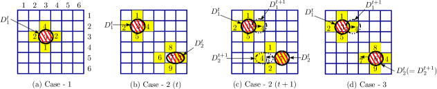
Figure 8: Design rules for pin-constrained DMFB: (a) Case-1 (b) Case-2 (at time $t$) (c) Case-2 (at time $t+1$) (d) Case-3

A general-purpose reconfigurable DMFB has a dedicated pin for controlling the actuations of each individual electrode. Hence, one can navigate each droplet to and from any electrode independently without affecting any other droplet sitting or moving elsewhere. As a trade-off between the flexibility of droplet movement and pin count, pin-constrained DMFBs [15, 16] may be deployed to reduce the number of control pins (single pin controls a group of electrodes) without affecting desired droplet movement.

Although earlier design methodologies [15, 16] can reduce the pin count significantly, they enforce several constraints on droplet movement. In this section, we describe the verification procedure for ensuring correct movement of two droplets on a pin-constrained DMFB. Moreover, for more than two droplets, one needs to consider the interference among them.

III-A Design rules for pin-constrained DMFB

The pin assignment problem satisfying the constraints for simultaneous movement of two or more droplets was studied earlier [15]. Our proposed verification scheme ensures that the fluidic instructions to be executed at time step $t$ satisfy all such constraints. Assume that $Pin(L)$ denotes the set of pins assigned to the electrodes of the set $L$ of cells, where $L\subseteq\{(x,y):1\leq x\leq r,1\leq y\leq c\}$, in a $(r\times c)$ DMFB. Let $N_{4}(x,y)$ denote the set of directly adjacent four neighbors of location $(x,y)$ as earlier. Let us consider now the design constraints on a case-by-case basis, assuming at $t$, the locations of two droplets are $D_{1}^{t}=(x_{1}^{t},y_{1}^{t})$ and $D_{2}^{t}=(x_{2}^{t},y_{2}^{t})$ respectively. At $t+1$, both droplets move by one cell and their locations become $D_{1}^{t+1}=(x_{1}^{t+1},y_{1}^{t+1})$ and $D_{2}^{t+1}=(x_{2}^{t+1},y_{2}^{t+1})$ respectively.

Case 1.

At any time instant, distinct pins are required to control the four neighborhood electrodes of any droplet. $\blacksquare$

Let a droplet be placed on location $(x^{t},y^{t})$ at time $t$. The above constraint can be modeled as follows.

$$\scriptsize Pin(\{(x_{1}^{t},y_{1}^{t})\})\bigcap_{\begin{subarray}{c}(x_{1}^{t},y_{1}^{t}),(x_{2}^{t},y_{2}^{t})\in N_{4}(x^{t},y^{t})\\ (x_{1}^{t},y_{1}^{t})\neq(x_{2}^{t},y_{2}^{t})\end{subarray}}Pin(\{(x_{2}^{t},y_{2}^{t})\})=\phi$$ (9)

This is needed to ensure possible movement of a droplet into its 4-neighborhood. This can be checked by analyzing the pairwise intersection of the electrode controlling pins of the 4-neighborhood of each droplet.

Example 8.

In Fig. 8(a), at time $t$, a droplet is placed on $(3,3)$. Note that $Pin(\{(3,3)\})=3$, $N_{4}(3,3)=\{(2,3),(3,2),(4,3),(3,4)\}$ and $Pin(\{(3,2)\})=Pin(\{(3,4)\})=2$. Hence, two opposite neighborhood electrodes of the droplet at $(3,3)$ share the same pin. This sharing will not cause any violation as long as pin 2 is inactive. In order to enable the left/right movement operation of the droplet at $(3,3)$, we need to activate pin 2 and deactivate pin 3 simultaneously. As a result, the droplet at $(3,3)$ will be split into two droplets unintentionally. Moreover, if two diagonal electrodes share the same pin, the droplet will be moved (instead of splitting) in between two diagonal electrodes that are controlled by the same pin. $\blacksquare$

Case 2.

At any time instant, the pin controlling the electrode of any droplet cannot be shared with any pins that control the 4-neighborhood electrodes of any other droplet. $\blacksquare$

In the case of $D_{1}^{t}$ and $D_{2}^{t}$, we can model the above constraint as:

$$(a):\>Pin(\{(x_{1}^{t},y_{1}^{t})\})\cap Pin(N_{4}(x_{2}^{t},y_{2}^{t}))=\phi$$ (10)

Interchanging the role of $D_{1}$ and $D_{2}$, we get

$$(b):\>Pin(N_{4}(x_{1}^{t},y_{1}^{t}))\cap Pin(\{(x_{2}^{t},y_{2}^{t})\})=\phi$$ (11)

Example 9.

In Fig. 8(b), two droplets are placed on $(2,2)$ and $(5,5)$ respectively, at time $t$. Note that $Pin(\{(2,2)\})=3$, $N_{4}(5,5)=\{(4,5),(5,4),(6,5),(5,6)\}$, $Pin(N_{4}(5,5))=\{8,6,9,3\}$. Hence, $Pin(\{(2,2)\})\cap Pin(N_{4}(5,5))=\{3\}$ i.e., at time $t$ one of the 4-neighbors of droplet $D_{2}^{t}$ shares the same pin $(3)$ of droplet $D_{1}^{t}$. Since both pins 3 and 7 are actuated with a high signal, $D_{2}^{t}$ may be unintentionally stretched and stay between electrodes $(5,5)$ and $(5,6)$. $\blacksquare$

Similarly at $t+1$, Case 2 can be encoded as:

$$(c):\>Pin(\{(x_{1}^{t+1},y_{1}^{t+1})\})\cap Pin(N_{4}(x_{2}^{t+1},y_{2}^{t+1}))=\phi$$ (12)

Interchanging the role of $D_{1}$ and $D_{2}$, we get

$$(d):\>Pin(N(x_{1}^{t+1},y_{1}^{t+1}))\cap Pin(\{(x_{2}^{t+1},y_{2}^{t+1})\})=\phi$$ (13)

Example 10.

Let us consider at time $t$, two droplets are placed on $(2,2)$ and $(5,5)$ and at $t+1$, they move to $(2,3)$ and $(5,4)$ respectively (Fig. 8(c)). Note that $Pin(\{(2,3)\})=4$, $N_{4}(5,4)=\{(4,4),(5,3),(6,4),(5,5)\}$, $Pin(N_{4}(5,4))=\{1,4,2,7\}$. Hence, $Pin(\{(2,3)\})\cap Pin(N_{4}(5,4))=\{4\}$, i.e., at time $t+1$, one of the 4-neighbors of droplet $D_{2}^{t+1}$ shares the same pin $(4)$ of droplet $D_{1}^{t+1}$. When both pin 4 and 6 are actuated with a high signal, $D_{2}^{t+1}$ may be unintentionally stretched and stay between the electrodes $(5,3)$ and $(5,4)$. $\blacksquare$

Case 3.

In order to move two droplets simultaneously at time instant $t+1$, the controlling pins of the destination electrodes, cannot be shared with any pins that control the 4-neighborhood electrodes of the other droplet at time $t$, except when the new locations of the two droplets share the same pin. $\blacksquare$

Hence, the movement constraint for $D_{1}^{t+1}$ and $D_{2}^{t+1}$ can be modeled as:

$$\footnotesize(a):\>Pin(\{(x_{1}^{t+1},y_{1}^{t+1})\})\cap Pin(N_{4}(x_{2}^{t},y_{2}^{t})\setminus\{(x_{2}^{t+1},y_{2}^{t+1})\})=\phi$$ (14)

Interchanging the roles of $D_{1}$ and $D_{2}$, we get the following constraint that needs to be honored as well:

$$\footnotesize(b):\>Pin(N_{4}(x_{1}^{t},y_{1}^{t})\setminus\{(x_{1}^{t+1},y_{1}^{t+1})\})\cap Pin(\{(x_{2}^{t+1},y_{2}^{t+1})\})=\phi$$ (15)

Example 11.

Assume, at time $t$, two droplets are placed on $(2,2)$ and $(5,5)$ and in the next time step i.e., at $t+1$, they move to $(2,3)$ and $(5,4)$ respectively. As shown in Fig. 8(d), $Pin(\{(2,3)\})=4,N_{4}(5,5)=\{(4,5),(5,4),(6,5),(5,6)\}$, $Pin(N_{4}(5,5)\setminus\{(5,4)\})=\{8,9,4\}$. Hence, $Pin(\{(2,3)\})\cap Pin(N_{4}(5,5)\setminus\{(5,4)\})=\{4\}$. Note that, at $t+1$, when $D_{2}^{t}$ tries to move from $(5,5)$ to $(5,4)$, pin 7, pin 6 and pin 4 are actuated with high, low and high signals respectively. As a consequence, $D_{2}^{t}$ is pulled with nearly equal forces from two adjacent high electrodes (controlled by pin 7 and pin 4) and cannot move as anticipated. However, at time $t+1$, if $D_{2}^{t}$ is moved to $(5,6)$ instead of $(5,4)$, then two droplets can be moved to their desired locations. $\blacksquare$

So far we have discussed the design constraints that need to be satisfied when two droplets move simultaneously. Additionally, we need to consider the design constraints when only one droplet moves and other remains at its location. However, this is a special case of simultaneous movement of two droplets. Without loss of generality, let us consider that the droplet $D_{2}^{t}$ remains in the same position at $t+1$, i.e., $D_{2}^{t+1}=D_{2}^{t}$. If we substitute $(x_{2}^{t},y_{2}^{t})$ by $(x_{2}^{t+1},y_{2}^{t+1})$ in the cases 2 and 3, we get six additional constraints that need to be satisfied when only one droplet moves and another remains static.

III-B Verifying fluidic operations on a pin-constrained DMFB

In this subsection, we describe the verification method for each fluidic instruction executed on a pin-constrained DMFB. We assume that the fluidic instructions executed at time $t$ do not violate any design constraints.

Dispense a reagent droplet – $d(i,j)$:

Before dispensing a reagent droplet, we need to ensure that it should not create any interference with other droplets present at $t$. This constraint can be verified by checking the intersection between the pin assigned to the electrode of the dispensed location $(i,j)$ and the pin assigned to the neighboring electrodes of each droplet. Moreover, the pin assigned to $(i,j)$ should not share any pin with its own neighbors. Otherwise, undesirable droplet stretching may occur.

Let there be $k$ droplets $\{(x_{1}^{t},y_{1}^{t}),(x_{2}^{t},y_{2}^{t}),\ldots,(x_{k}^{t},y_{k}^{t})\}$ present on a DMFB at time $t$. At $t+1$, a droplet is dispensed from a reagent reservoir to location $(i,j)$. If $Pin(\{(i,j)\})\cap Pin(N_{4}(x_{l}^{t},y_{l}^{t}))=\phi$, for $l=1,2,\ldots,k$ and $Pin(\{(i,j)\})\cap Pin(N_{4}(i,j))=\phi$, it is safe to dispense a droplet on $(i,j)$ at time $t+1$.

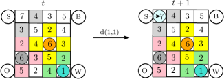
Figure 9: Verifying the dispense operation

Example 12.

Assume at time $t$, three droplets are present at locations $(3,3),(4,1)$ and $(5,4)$ (Fig. 9). It is easy to check that at time $t$, there are no violations, and a droplet can be dispensed on $(1,1)$ at time $t+1$. $Pin(N_{4}(3,3))=\{2,4,5,3\}$, $Pin(N_{4}(4,1))=\{2,5,3\}$, $Pin(N_{4}(5,4))=\{2,4\}$ and $Pin(N_{4}(1,1))=\{3,4\}$. Hence, the pin assigned to $(1,1)$ is disjoint with the set of pins assigned to its own neighbors and the neighbors of other droplets, i.e., $\{7\}\cap\{2,4,5,3\}=\phi$, $\{7\}\cap\{2,5,3\}=\phi$, $\{7\}\cap\{2,4\}=\phi$, $\{7\}\cap\{3,4\}=\phi$. Hence, the reagent droplet can be safely dispensed on $(1,1)$ at $t+1$.

If at $t+1$, a droplet is dispensed to $(1,4)$ instead of $(1,1)$, we have a violation. Note that, the pin assigned to $(1,4)$ has a non-null intersection with $Pin(N_{4}(3,3))$ and $Pin(N_{4}(4,1))$. Hence, droplet stretching may occur. $\blacksquare$

Transporting a droplet to a waste reservoir – $waste(i,j)$:

This case is straightforward. We need to ensure that the waste droplet to be transported at $t+1$ must not share any pin with other droplets present at time $t$. This fact is true because at $t$, no design constraint was violated.

Transporting a droplet to an output reservoir – $output(i,j)$:

This is similar to $waste(i,j)$.

Transportation of a droplet – $m([r_{1},c_{1}]\to[r_{2},c_{2}])$:

The correctness checking of concurrent droplet movements can be decomposed into checking for all possible pairs of droplet movement. In fact, the verification of simultaneous movement of a pair of droplets on a pin-constrained DMFB is equivalent to checking Cases 1-3. Note that we have to check Case-2 only for time instant $t+1$, because at time $t$, all constraints are satisfied. Moreover, we can suitably modify Cases 2-3 for verifying the instance when only one droplet is moved and the other remains static. The next example illustrates this scenario.

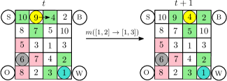
Figure 10: Verifying move operation on pin-constrained DMFB

Example 13.

Suppose, at time $t$, three droplets are present on locations $(1,2),(4,1)$ and $(5,4)$ respectively. At $t+1$, $m([1,2]\rightarrow[1,3])$ will be executed, i.e., droplet at $(1,2)$ will be moved to its right neighbor at $(1,3)$ and other droplets will not move. Note that $Pin(\{(1,2)\})=\{9\},Pin(N_{4}(1,2))=\{10,7,4\},Pin(N_{4}(1,3))=\{9,5,2\}$ and $Pin(\{(4,1)\})=\{6\},Pin(N_{4}(4,1))=\{5,8,7\}$. It can be easily verified that the constraint in Case 1 is satisfied. The following cases (Case 2 and Case 3) must be satisfied for checking interference of moving droplet with the static droplet on $(4,1)$.

Cases:

• $Pin(\{(1,3\})\cap Pin(N_{4}(4,1))=\{4\}\cap\{5,8,7\}=\phi$

• $Pin(N_{4}(1,3))\cap Pin(\{(4,1)\})=\{9,5,2\}\cap\{6\}=\phi$

• $Pin(\{(1,3)\})\cap Pin(N_{4}(4,1)\setminus\{(4,1)\})=\{4\}\cap\{5,8,7\}=\phi$

• $Pin(N_{4}(1,2)\setminus\{(1,3)\})\cap Pin(\{(4,1)\})=\{10,7\}\cap\{6\}=\phi$

Similar checking is required for another static droplet on $(5,4)$. It is interesting to notice that if $m([1,2]\rightarrow[2,2])$ is executed instead of $m([1,2]\rightarrow[1,3])$, it violates the design constraint, since $Pin(\{(2,2)\})\cap Pin(N_{4}(4,1))=\{7\}\cap\{5,8,7\}\neq\phi$. $\blacksquare$

Mixing operation – $mix([r_{1},c_{1}]\leftrightarrow[r_{2},c_{2}],t_{mix},mtype$):

Correctness checking of a mixing operation depends on the type of the mixer used since different mixers have different sizes and mixing times. Design methodologies for assay specific pin-constrained DMFB [15] assign pins for independent mixer units in such a manner so that mixers can operate in parallel. However, assay-independent pin assignments require correctness checking of the mixing operation at each time step. Note that one can easily split the mixing operation into a sequence of move operations over time. Again it depends on the type of mixer and running time. For simplicity, we have assumed that mixers are instantiated at particular locations on the DMFB and their pin assignments are independent.

IV The complete verification procedure

We will now illustrate the design constraint verification process on an example of diluting a sample using twoWayMix [9]. The symbolic form of the synthesized output (actuation sequences) is also shown in Fig. 3. The snapshot of the biochip at different time instants is shown in Fig. 4. The design constraint analysis process reads the symbolic fluidic instructions and verifies the operations to be executed at time $t+1$ (if any), depending upon the biochip description at $t$, i.e., $B_{r\times c}^{t}$.

Let us assume that we have set up $T_{reservior}$ from architectural descriptions correctly, and initialized the biochip status at $t=0$, i.e., $B_{r\times c}^{0}(=\wedge_{(\forall i,j)}\neg x_{i,j}^{0})$ and set $T_{mixer}=\phi$. In the next time step $(t+1)$, $T_{mixer}$ is checked for any expired mixer. If yes, we need to take an appropriate action described in the $mix$ operation of Section II. Next, the fluidic operations $(I_{t+1})$, which are to be executed at $t+1$ are taken care of. Each instruction is verified as stated earlier and $B_{r\times c}^{t+1}$ is updated gradually. Finally, when all the executable instructions at $t+1$ are verified, $B_{r\times c}^{t+1}$ is evaluated for truth value. If it is true, we proceed to the next time step and continue this process until all actuation sequences are processed. If any fluidic instruction executed at any instant violates any design constraint, the potential cause is notified for debugging purpose.

Correctness of synthesized sequencing graph

The synthesized bioassay, which is verified to have no design errors, might still suffer from certain realization errors. Hence, we explicitly construct the synthesized sequencing graph with the design constraint analysis process. Once we reconstruct a complete sequencing graph on successful completion of the design analysis phase, it is compared with the input graph for detecting realization errors, if any. The outline of the incremental construction of synthesized sequencing graph is as follows.

We assign an unique $id$ to each droplet, input reagent, output and waste reservoir and graph $G_{s}=(V_{s},E_{s})$ is created, where $V_{s}$ contains the nodes labeled with reservoir $id$s and $E_{s}=\phi$. Any droplet dispensed from a reservoir inherits the same $id$ as that of the dispensing reservoir and retains it while movement during its lifetime. The mix operation is handled in a different fashion. Note that it requires the insertion of an entry in $T_{mixer}$, which contains the $id$s of two input droplets along with start ($t_{s}$) and end ($t_{e}$) time of mixing operation. When a mixing operation is completed, two new droplets are created. A unique $id_{new}$ is generated and assigned to both of these droplets. A new node $v_{new}$ labeled with $id_{new}$ is added to $V_{s}$, and two edges $(v_{1},v_{new})$ and $(v_{2},v_{new})$ are added to $E_{s}$, where $id$s of $v_{1}$ and $v_{2}$ are the $id$s of droplets that were mixed together. Additionally, we store the start and end times of mixing operation in $v_{new}$. Similarly, when a droplet is transported to an output or to a waste reservoir, an edge is created to indicate the dispense operation. The following example illustrates the generation of synthesized sequencing graph with design constraint analysis.

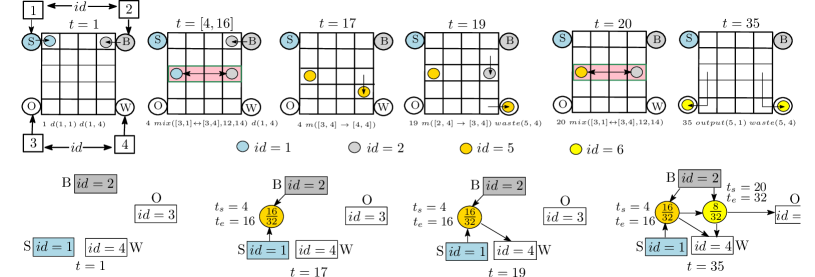
Figure 11: Incremental construction of the synthesized sequencing graph

Example 14.

Consider the bioassay as shown in Fig. 3. The snapshots of the layout and the sequencing graph, which is incrementally reconstructed over different time steps, are shown in Fig. 11. Initially, we assign unique $id$s to the sample and buffer dispensers, output and waste reservoirs as $id$ 1 and 2, 3 and 4 respectively. A directed graph $G_{s}=(V_{s},E_{s})$, where $V_{s}=\{S,B,O,W\}$ and $E_{s}=\phi$, is created. At $t=0$, two droplets are dispensed from the sample and buffer reservoirs respectively. A mixer is instantiated with two droplets i.e., sample $(id=1)$ and buffer $(id=2)$, at $t=4$ which remains active until $t=17$. At $t=17$, two new droplets are created by mixing sample with buffer and a new $id\>(5)$ is assigned to each of the newly generated droplets. Moreover, a new node with concentration factor $\frac{16}{32}$ is added along with two edges i.e., $V_{s}=V_{s}\cup\{v_{1}\}$ and $E_{s}=E_{s}\cup\{(S,v_{1}),(B,v_{1})\}$. Note that the newly created node $v_{1}$ is annotated with mixing start time ($t_{s}$) and end time ($t_{e}$). At $t=19$, the droplet with $id=5$ is moved to the waste reservoir, which in effect adds a new edge to $E_{s}$ i.e., $E_{s}=E_{s}\cup\{(v_{1},W)\}$. Another mixer, which is instantiated at $t=20$, can be handled analogously. The synthesized sequencing graph is generated at $t=35$ as shown in Fig. 11. $\blacksquare$

After the synthesized sequencing graph is generated and annotated with concentration factors/ratios, its conformance with the input sequencing graph is easy to check. Two dummy nodes $v_{start}$ and $v_{end}$ are added to make each of them a single-entry and a single-exit graph. Since the start and end times of each mix operation are available from the corresponding node, it is easy to compute the mixing time. Also, the concentration factors/ratios of the droplets are known, and therefore, a breadth-first traversal on the two graphs is enough for checking the correspondence between them. However, if there was a realization error (e.g., because of a wrong mix-split operation), then a different concentration factor/ratio would have been generated. Hence, the proposed graph traversal can identify such unintended mixing operations.

V Implementation

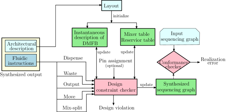
Figure 12: Architecture of the verification engine

We have developed a DMF biochip simulator (SimBioSys) and integrated with the verification engine for visual simulation of a complete assay operation. The architecture of our verification tool is shown in Fig. 12. It has two major components, namely, a design-constraint checker and a conformance checker.

The design-constraint checker takes the symbolic representation of the synthesized output as one of the inputs and extracts the architectural layout parameters (dimension, reservoirs) on which the synthesized bioassay will be executed. After extracting the DMFB layout, it initializes the reservoir table and the associated data structure for maintaining the instantaneous description of the DMFB with no droplet present at time $t=0$. Similarly, the mixer table is initialized. Next, the design-constraint checker reads the fluidic instructions to be executed at time $t+1$ and groups them into several fluidic instruction categories as shown in Fig. 12. Note that the fluidic instructions executed at time $t+1$ are concurrent. The verification engine checks the correctness of instructions in each group and generates the potential cause of design rule violation along with the fluidic operation that might have caused the violation.

Note that the Boolean expressions that capture the design constraints described in Section II are simple in nature i.e., each CNF clause consists of only one variable. Hence, truth-value checking can be accomplished without invoking any sophisticated satisfiability (SAT) solver. We need a constraint solver that can take in a Boolean formula and a valuation to the variables, and determine if the formula evaluates to $true$ or $false$. This is more of verifying a witness on a Boolean formula (polynomial time), than generating a witness (computationally hard). We have used a table-driven method that determines the truth value of Boolean expressions in $O(r\times c)$ time, i.e., linear in the number of electrodes in the biochip. In the case of the pin-constrained biochip verification process, the design-constraint checker takes the pin assignment separately and checks the pin constraint specific design rules which are described in Section III. Additionally, it incrementally builds the annotated synthesized sequencing graph. Finally, conformance checking between the synthesized sequencing graph and input sequencing graph is performed. If any realization error is detected by the checker, it is notified to the user along with the potential cause of violation.

VI Case studies

We have tested our framework on two real-life biochemical assays, namely, the polymerase chain reaction (PCR) protocol [17] and the multiplexed bioassay [15]. A general-purpose DMFB is used for verifying PCR whereas a pin-constrained DMFB platform is used for correctness checking of the multiplexed bioassay. In our experiments, we injected several design and realization errors in the synthesized output and observed the response of the tool.

PCR on a general-purpose DMFB

(a) Mixing stage of PCR

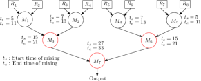
(b) Synthesized PCR mixing tree

Figure 13: Behavioral description of bioassay.

TABLE I: Symbolic representation of the actuation sequence of PCR

Architectural layout
$dim(15,15)$ $accuracy\>\>5$
$R(3,1,R_{1})\>R(8,1,R_{2})\>R(13,1,R_{3})\>R(15,8,R_{4})\>R(1,8,R_{5})\>R(3,15,R_{6})\>R(8,15,R_{7})\>R(13,15,R_{8})$
$t$	Symbolic instructions executed
1	$d(3,1)$ $d(8,1)$ $d(13,1)$ $d(15,8)$ $d(13,15)$ $d(8,15)$ $d(3,15)$ $d(1,8)$
2	$m([3,1]\to[3,2])$ $m([8,1]\to[8,2])$ $m([13,1]\to[13,2])$ $m([15,8]\to[14,8])$ $m([13,15]\to[13,14])$ $m([8,15]\to[8,14])$ $m([3,15]\to[3,14])$ $m([1,8]\to[2,8])$
3	$m([3,2]\to[3,3])$ $m([8,2]\to[8,3])$ $m([13,2]\to[13,3])$ $m([14,8]\to[13,8])m([13,14]\to[13,13])$ $m([8,14]\to[8,13])$ $m([3,14]\to[3,13])$ $m([2,8]\to[3,8])$
4	$m([3,3]\to[4,3])$ $m([8,3]\to[7,3])$ $m([13,3]\to[12,3])$ $m([13,8]\to[12,8])m([13,13]\to[12,13])$ $m([8,13]\to[9,13])$ $m([3,13]\to[4,13])$ $m([3,8]\to[4,8])$
5	$mix([4,3]\leftrightarrow[7,3],6,41)$ $mix([9,13]\leftrightarrow[12,13],6,41)$ $m([12,3]\to[11,3])$ $m([12,8]\to[11,8])$ $m([4,13]\to[5,13])$ $m([4,8]\to[5,8])$
6	$m([11,3]\to[11,4])$ $m([11,8]\to[11,7])$ $m([5,13]\to[5,12])$ $m([5,8]\to[5,9])$
7	$mix([11,4]\leftrightarrow[11,7],6,14)$ $mix([5,12]\leftrightarrow[5,9],6,14)$
14	$m([4,3]\to[3,3])$ $m([7,3]\to[8,3])$ $m([11,4]\to[11,3])$ $m([11,7]\to[11,8])m([12,13]\to[13,13])$ $m([9,13]\to[8,13])$ $m([5,12]\to[5,13])$ $m([5,9]\to[5,8])$
15	$mix([8,3]\leftrightarrow[11,3],6,41)$ $mix([8,13]\leftrightarrow[5,13],6,41)$ $m([5,8]\to[4,8])$ $m([11,8]\to[12,8])$
22	$m([8,3]\to[7,3])$ $m([11,3]\to[11,4])$ $m([12,8]\to[13,8])$ $m([8,13]\to[9,13])m([5,13]\to[5,12])$ $m([4,8]\to[3,8])$
23	$m([7,3]\to[6,3])$ $m([11,4]\to[11,5])$ $m([9,13]\to[10,13])$ $m([5,12]\to[5,11])$
24	$m([6,3]\to[5,3])$ $m([11,5]\to[11,6])$ $m([10,13]\to[11,13])$ $m([5,11]\to[5,10])$
25	$m([5,3]\to[5,4])$ $m([11,6]\to[11,7])$ $m([11,13]\to[11,12])$ $m([5,10]\to[5,9])$
26	$m([5,4]\to[5,5])$ $m([11,7]\to[11,8])$ $m([11,12]\to[11,11])$ $m([5,9]\to[5,8])$
27	$mix([5,5]\leftrightarrow[5,8],6,14)$
34	$end$

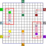
(a) $t=[1,5]$

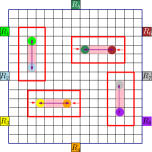
(b) $t=[6,7]$

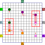
(c) $t=[14,15]$

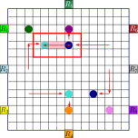
(d) $t=[22,27]$

Figure 14: Snapshot of the execution of synthesized PCR mixing tree

The polymerase chain reaction is one of the most common techniques for rapid enzymatic amplification of specific DNA fragments using temperature cycles [17]. Here, we use the mixing stage of PCR as an example to evaluate our verification tool. The sequencing graph [18] of the PCR mixing steps is shown in Fig. 13(a) and the symbolic representation of the synthesized outputs [18] is shown in Table I. Fig. 14 shows the DMFB description at different time instants along with droplet paths and mixer instantiations.

A snapshot of SimBioSys simulating the PCR protocol can be found in [1] . Any design/realization constraint violation can be easily localized by running SimBioSys. Some results on the PCR protocol are reported in Table LABEL:tab:test-results-pcr. Several design errors ($e_{i}$), listed in Table LABEL:tab:design-error, are injected into the symbolic form of the synthesized output. The corresponding responses of the verification tool are listed in Table LABEL:tab:test-results-pcr. In each case, a potential cause was identified correctly, and the corresponding fluidic violations were properly listed.

[ caption = Experimental results for erroneous PCR mixing, label = tab:test-results-pcr, pos = !h, width = 0.5framesep=0pt, framerule = 1pt, doinside = ]p5ptp120ptp1ptp73pt Phase I - Design constraint checking Response of SimBioSys t Instruction causing violation $e_{1}$ Static fluidic constraint violated 27 $m(11,8,12,8)$ $e_{2}$ Dynamic fluidic constraint violated 26 $m(11,7,11,8)$ $m(13,8,12,8)$ $e_{3}$ Dispense from invalid input reservoir 1 $d(2,1)$ $e_{4}$ Droplet on (5,5) is in active mixer 28 $m(5,5,5,4)$ $e_{5}$ Droplet is not present on (11,4) and (11,7) 6 $mix(11,4,11,7,6,14)$ Phase II - Realization error checking Response of SimBioSys Potential cause of error $e_{6}$ Inhomogeneous mixing Mixing performed for lesser time $e_{7}$ Incorrect realization of input sequencing graph Wrong mix operation performed

Multiplexed bioassay on a pin-constrained DMFB

Digital microfluidic platforms have been successfully used [19] for in-vitro measurement of glucose and other metabolites, such as lactate, glutamate, and pyruvate, in human physiological fluids. Hence, an in-vitro multiplexed bioassay for detecting human metabolic disorders has immense importance in real life. We demonstrate our verification protocol for such a multiplexed bioassay running on a pin-constrained DMFB. The layout and the pin assignment [15] of DMFB are shown in Fig. 15.

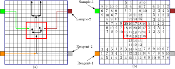
Figure 15: Multiplexed bioassay (a) DMFB layout (b) Pin assignment

We have verified the synthesized bioassay using a general purpose DMFB (dedicated pin for each electrode) in order to ensure that the synthesized bioassay is free from any design or realization errors except those that appear from constrained pin assignments. Although this requirement is not mandatory, we assume it for showing only errors related to pin assignment. As earlier, we injected several errors into the pin assignment of the DMFB and observed the response of the verification engine. The corresponding responses of the verification tool are listed in Table LABEL:tab:test-results-mplex. Note that in the first column, we have listed the new pin assignment of the cells that is modified to introduce errors in the pin assignment shown in Fig. 15(b). In every case, the consequences of pin assignment over fluidic instructions are detected along with the fluidic operation that triggers the violation.

[ caption = Experimental results on pin-constrained DMFB, label = tab:test-results-mplex, pos = !h, width = 0.48framesep=0pt, framerule = 1pt, doinside = ]p73ptp74ptp1ptp76pt Pin assignment &Verifier response t Instructions$Pin(\{(13,5)\})=6$ Droplet stretch 4 $m(3,3,4,3)$ $m(13,3,13,4)$$Pin(\{(13,15)\})=8$, $Pin(\{(14,15)\})=10$ Droplet stuck on $(13,14)$ 53 $m(13,14,13,13)$ $m(3,14,3,13)$$Pin(\{(6,13)\})=7$ Droplet stuck on $(13,11)$ 56 $m(5,13,6,13)$ $m(13,11,13,10)$

VII Verifying fault-tolerant biochemical protocols on a cyberphysical DMFB

We now describe how the proposed framework can be used to verify the correctness of a fault-tolerant implementation of an input sequencing graph. Because of the intrinsic errors prevalent in common microfluidic operations, several fault-tolerant synthesis methodologies [20, 21, 13] were proposed. In such a cyberphysical system, on-chip optical or electronic sensors check for the presence of any volumetric/concentration error in the droplets, and their feedback is used to govern the assay operations in real-time. Synthesis tools for such implementations of the input sequencing graph $(G)$ insert detection operation for appropriate droplets in $G$. It also generates recovery operations a-priori for handling any detected errors. Fig. 16 (a) shows the input sequencing graph $(G)$ to be implemented on an $8\times 8$ DMFB platform (Fig. 16 (b)). A synthesis tool inserts two detection operations on the output droplets of mixers $M_{1}$ and $M_{2}$ in $G$, resulting in the sequencing graph G+ (Fig. 16(d)). We assume that no faults can occur more than once.

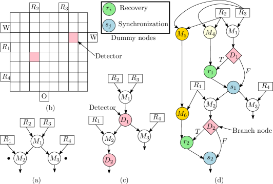
Figure 16: (a) DMF platform (b) Input sequencing graph $(G)$ (c) Fault-tolerant sequencing graph graph $(G^{+})$ (d) Sequencing graph implementing $G^{+}$

We need to augment our proposed instruction set (Table LABEL:tab:instructions) with new instructions for dealing with error detection and recovery in a fault-tolerant implementation of $G$. The on-chip optical detectors are encoded as $D(d_{i},x,y,t)$, where $(x,y)$ is the location of the detector, $d_{i}$ is an unique identifier and $t$ denotes the number of cycles required for detection. Additionally, fluidic operation $detect(d_{i})$ starts the on-chip detector $d_{i}$, and after the detection, the corresponding flag in the DMFB controller memory is set appropriately [21]. Based on the error flag value of $d_{i}$, $if(d_{i})\>\>\>call<Recovery(j)>$ instruction conditionally jumps to the recovery routine $Recovery(j)$, where the parameter $j$ provides a pointer to an appropriate error-handling routine.

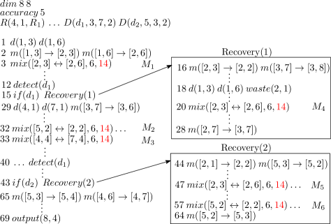
Figure 17: Synthesized output with error recovery routines

Example 15.

Fig. 17 shows the actuation sequence generated by the synthesis tool implementing Fig. 16(d) when errors are detected in the droplets generated from the mixing operations $M_{1}$ and $M_{2}$. Note that at $t=15$, error recovery actions are performed ($Recovery(1)$ repeats mixing operation $M_{1}$ with a new mixing operation $M_{4}$); at $t=28$, the recovery finishes. Similarly, $Recovery(2)$ instantiates two new mixing operations $M_{5}$ and $M_{6}$ in order to recover the error detected by detector $D_{2}$. $\blacksquare$

The fluidic instructions to be executed in the synthesized bioassay depend upon the detection results. Depending on the outcomes of the two detectors (Fig. 16(d)), there can be four possible ways the input bioassay can be executed. However, for verifying its correct implementation, we need to ensure the correctness for each of the possible execution paths. Hence, the complexity of the verification problem may grow exponentially in such a cyberphysical scenario.

Our verification method symbolically traverses through a valid snapshot of the DMFB at time instant $t$, i.e., $(B_{r\times c}^{t})$ to construct another valid snapshot at $t+1$, i.e., $(B_{r\times c}^{t+1})$, this is accomplished by checking the correctness of the fluidic instructions to be executed at $t$ on $(B_{r\times c}^{t})$. However, in the incremental verification process, conditional jump instructions $(if)$ may require special consideration. Let us consider the actuation sequence shown in Fig. 17. Note that at $t=15$, depending on the detection result, the controller decides whether it needs to start an error recovery operation $(Recovery(1))$, or continue with normal execution (instructions following $if$). Hence, two separate streams of fluidic instructions can be executed at time instant $t=16$, i.e., those from $Recovery(1)$, or those to be executed at $t=29$ in Fig. 17. It is important to note that Fig. 17 shows the actuations when the droplets generated from $M_{1}$ and $M_{2}$ are erroneous. The controller appropriately fires the desired instruction stream [21] depending on the detection outcome without any unnecessary delay. Hence at $t=16$, two valid snapshots are possible depending on the two instruction streams. Analogously, when the next $if$ instruction is encountered (at $t=43$ in Fig. 17), four separate valid execution paths are generated depending on the two instruction streams for each of the previous two valid snapshots. Thus, formally, the possible execution paths can be encoded as:

$$B_{8\times 8}^{0}\ldots B_{8\times 8}^{14}(B_{8\times 8}^{15}+B_{8\times 8}^{16}\ldots B_{8\times 8}^{28})$$

$$B_{8\times 8}^{29}\ldots B_{8\times 8}^{42}(B_{8\times 8}^{43}+B_{8\times 8}^{44}\ldots B_{8\times 8}^{64})B_{8\times 8}^{65}\ldots B_{8\times 8}^{69}$$

The notation $B_{8\times 8}^{0}\ldots B_{8\times 8}^{14}B_{8\times 8}^{15}B_{8\times 8}^{29}\ldots B_{8\times 8}^{42}B_{8\times 8}^{43}B_{8\times 8}^{65}\ldots\\ \ldots B_{8\times 8}^{69}$ denotes the normal execution path where the transition from $B_{8\times 8}^{15}$ to $B_{8\times 8}^{29}$ happens for set of fluidic operations at time instant 29 (Fig. 17). We can thus verify all the fluidic instructions along each of the valid execution paths using the framework discussed in Section II. When all such paths are verified for any design error, the $SG$ is reconstructed as before for the detection of realization errors, if any. In certain situations, it may also be possible to check the correctness of only the actual data path just before its execution at run-time.

VIII Conclusion and future directions

We have presented the foundations of a formal correctness checking framework for post-synthesis verification of a biochemical mixing protocol implemented on a DMF platform. Our formulation allows us to model several possible sources of design and implementation errors that may arise in the design of general-purpose, pin-constrained and cyberphysical biochips. The verification flow has been formalized and tested on the PCR protocols and in-vitro multiplexed bioassay. To the best of our knowledge, such a framework does not exist in the literature. It paves the way of handling several violations that may arise from imprecise synthesis strategies and change in target architectures. The study also opens up several new challenges concerning on-chip protocol realizations. In particular, the generalization of the method for incorporating verification of a technology-enhanced chip remains open.

References

- [1] S. Bhattacharjee, A. Banerjee, K. Chakrabarty, and B. B. Bhattacharya, “Correctness checking of bio-chemical protocol realizations on a digital microfluidic biochip,” in Proc. VLSI Design, Jan. 2014, pp. 504–509.
- [2] M. J. Jebrail and A. R. Wheeler, “Let’s get digital: digitizing chemical biology with microfluidics,” Current Opinion in Chemical Biology, vol. 14, no. 5, pp. 574–581, 2010.
- [3] D. Grissom, K. O’Neal, B. Preciado, H. Patel, R. Doherty, N. Liao, and P. Brisk, “A digital microfluidic biochip synthesis framework,” in Proc. VLSI-SoC, 2012, pp. 177–182.
- [4] O. Keszocze, R. Wille, T.-Y. Ho, and R. Drechsler, “Exact one-pass synthesis of digital microfluidic biochips,” in Proc. DAC, 2014, pp. 1–6.
- [5] D. Grissom, C. Curtis, and P. Brisk, “Interpreting assays with control flow on digital microfluidic biochips,” JETC, vol. 10, no. 3, pp. 1–30, 2014.
- [6] T. Zhang, K. Chakrabarty, and R. B. Fair, Microelectrofluidic Systems - Modeling and Simulation. CRC Press, 2002.
- [7] J. McDaniel, A. Baez, B. Crites, A. Tammewar, and P. Brisk, “Design and verification tools for continuous fluid flow-based microfluidic devices,” in Proc. ASP-DAC, 2013, pp. 219–224.
- [8] M. Aagaard and M. Leeser, “A formally verified system for logic synthesis,” in Proc. ICCD, 1991, pp. 346–350.
- [9] D. Mitra, S. Roy, S. Bhattacharjee, K. Chakrabarty, and B. B. Bhattacharya, “On-chip sample preparation for multiple targets using digital microfluidics,” IEEE Trans. on CAD of Integrated Circuits and Systems, vol. 33, no. 8, pp. 1131–1144, 2014.
- [10] K. Chakrabarty and F. Su, Digital Microfluidic Biochips - Synthesis, Testing, and Reconfiguration Techniques. CRC Press, 2007.
- [11] F. Su, W. L. Hwang, and K. Chakrabarty, “Droplet routing in the synthesis of digital microfluidic biochips,” in Proc. DATE, 2006, pp. 323–328.
- [12] M. Schertzer, “Characterization of the motion and mixing of droplets in electrowetting on dielectric devices,” Ph.D. dissertation, University of Toronto, 2010.
- [13] Y. Luo, K. Chakrabarty, and T.-Y. Ho, “Error recovery in cyberphysical digital microfluidic biochips,” IEEE Trans. on CAD of Integrated Circuits and Systems, vol. 32, no. 1, pp. 59–72, 2013.
- [14] S. Park, P. A. L. Wijethunga, H. Moon, and B. Han, “On-chip characterization of cryoprotective agent mixtures using an ewod-based digital microfluidic device,” Lab on a Chip, vol. 11, pp. 2212–2221, 2011.
- [15] T. Xu, W. L. Hwang, F. Su, and K. Chakrabarty, “Automated design of pin-constrained digital microfluidic biochips under droplet-interference constraints,” JETC, vol. 3, no. 3, 2007.
- [16] Y. Luo and K. Chakrabarty, “Design of pin-constrained general-purpose digital microfluidic biochips,” IEEE Trans. on CAD of Integrated Circuits and Systems, vol. 32, no. 9, pp. 1307–1320, 2013.
- [17] S. Roy, S. Kumar, P. P. Chakrabarti, B. B. Bhattacharya, and K. Chakrabarty, “Demand-driven mixture preparation and droplet streaming using digital microfluidic biochips,” in Proc. DAC, 2014, pp. 1–6.
- [18] F. Su and K. Chakrabarty, “Module placement for fault-tolerant microfluidics-based biochips,” ACM Trans. Des. Autom. Electron. Syst., vol. 11, no. 3, pp. 682–710, June 2004.
- [19] R. Sista, Z. Hua, P. Thwar, A. Sudarsan, V. Srinivasan, A. Eckhardt, M. Pollack, and V. Pamula, “Development of a digital microfluidic platform for point of care testing,” Lab Chip, vol. 8, no. 12, pp. 2091–2104, Dec. 2008.
- [20] M. Alistar, P. Pop, and J. Madsen, “Online synthesis for error recovery in digital microfluidic biochips with operation variability,” in Proc. DTIP, 2012, pp. 53–58.
- [21] Y. Zhao, T. Xu, and K. Chakrabarty, “Integrated control-path design and error recovery in the synthesis of digital microfluidic lab-on-chip,” JETC, vol. 6, no. 3, 2010.