LGSQE: Lightweight Generated Sample Quality Evaluation

Abstract

Despite prolific work on evaluating generative models, little research has been done on the quality evaluation of an individual generated sample. To address this problem, a lightweight generated sample quality evaluation (LGSQE) method is proposed in this work. In the training stage of LGSQE, a binary classifier is trained on real and synthetic samples, where real and synthetic data are labeled by 0 and 1, respectively. In the inference stage, the classifier assigns soft labels (ranging from 0 to 1) to each generated sample. The value of soft label indicates the quality level; namely, the quality is better if its soft label is closer to 0. LGSQE can serve as a post-processing module for quality control. Furthermore, LGSQE can be used to evaluate the performance of generative models, such as accuracy, AUC, precision and recall, by aggregating sample-level quality. Experiments are conducted on CIFAR-10 and MNIST to demonstrate that LGSQE can preserve the same performance rank order as that predicted by the Fréchet Inception Distance (FID) but with significantly lower complexity.

Index Terms—  Generative Models, Quality Evaluation, Green Learning

1 Introduction

Evaluation of image generative models has become an active research topic due to the rapid advances in adversarial and non-adversarial generative models. Advanced image generative models find applications in image generation, image inpainting, image-to-image translation, etc. Due to the popularity of generative models, it is essential to have an automatic means to measure the quality of generated samples in an objective way without involving the human subjective test.

Quite a few quantitative metrics have been proposed in recent years [1, 2]. Examples include the Inception Score (IS) [3], the Fréchet Inception Distance (FID) [4], the Classifier two-sample test [5] and the Precision and Recall (P&R) [6], etc. Each metric has its own strengths and weaknesses. Although being popular, the aforementioned evaluation methods share two common issues. First, they measure the effectiveness of a generative model based on the statistics of its whole generated samples. They cannot be applied to a single generated sample. In certain applications, it is desired to assess the quality of individual samples on the fly in the absence of ensemble distributions. Second, an important aspect for an evaluation method is its computational complexity. Some methods rely on deep features obtained from late layers of deep neural networks (DNNs). As a result, their computational complexity and memory cost are high. Also, certain evaluation methods are biased towards the ImageNet that is commonly adopted in pre-trained networks. Although efforts have been made to develop better quality evaluation methods, e.g. [7, 8, 9], these two fundamental problems still exist.

A lightweight generated sample quality evaluation (LGSQE) method is proposed to address them in this work. LGSQE trains a binary classifier to differentiate real and synthetic samples generated by a generative model. In the training stage, real and generated samples are assigned with labels “zero” and “one”, respectively. In the testing stage, a soft label is obtained, which serves as its quality index. The sample quality is good (or bad) if its soft label is farther away from (or close to) one. The LGSQE pipeline consists of three steps: 1) design a simple yet effective representation for real/synthetic images from a source dataset, 2) determine discriminant features, and 3) conduct binary classification.

As a byproduct, LGSQE can provide quality metrics for a generative model by aggregating quality indices of a large number of generated samples. Intuitively, a poorly-performing generative model tends to yield more bad samples. The distribution of generated samples from a poorly-performing generative model is quite different from that of real samples in the sample representation space. The accuracy of the binary classifier is higher since their distributions are more separable. In contrast, if the classification performance is close to chance level (i.e., half-half), it indicates a high-performing model that generates high-quality samples that are close to the real ones in the representation space. LGSQE is a dataset-specific method. The dataset chosen as the generation target (e.g., CIFAR-10, etc.) is used to train LGSQE from scratch, as implemented in Step 1. It is worth noting existing quality metrics for generative models are all not dataset-specific.

The rest of this paper is organized as follows. Related work is briefly reviewed in Sec. 2. The LGSQE method is presented in Sec. 3. Experimental results are shown in Sec. 4. Concluding remarks and future research directions are given in Sec. 5.

2 Related Work

Quite a few metrics for generative model evaluation have been proposed. They are reviewed in Sec. 2.1. Furthermore, we conduct a brief survey on recent development in green learning in Sec. 2.2, as it pertains to the representation learning and feature selection of the proposed LGSQE method.

2.1 Evaluation Metrics for Generative Models

The Inception Score (IS) [3] is one of the early developed metrics. It uses the Inception-Net pre-trained on ImageNet to calculate the KL-divergence between the conditional and marginal distributions. It has some limitations. First, it is susceptible to overfit [10]. Second, it fails to account for the mode collapse problem with generative models and its bias towards ImageNet may give an image quality assessment in an object-wise manner (rather than realistically-wise one). Third, it is sensitive to the image resolution and not being a proper distance metric.

The Fréchet Inception Distance (FID) [4] is meant to improve deficiencies of IS. Inception-V3 is used to map samples onto its embedding space, where real and synthetic samples are modeled by joint Gaussian distributions. FID improves over IS by accounting for intra-class mode dropping and in turn the diversity of generated samples between models. Yet, the log-likelihood distributions between real and synthesized samples are not easy to be captured in the high dimensional feature space [11]. FID is further enhanced in [12] by introducing the Class-Aware Frechet Distance (CAFD).

The precision-recall metric with a reference data manifold was introduced in [13]. It attempts to take both fidelity and diversity into account. Yet, it has a bottleneck in real applications; namely, it is impractical to be deployed since the reference manifold is not available in most settings. Other reported limitations include failure to realize the match between identical distributions and robustness to outliers [9].

Another line of research adopts classifier-based evaluation [8] by training a classifier on real and synthetic samples. The classifier plays the role of a discriminator, and its error rate is used for performance assessment. For instance, the two-sample test [5] adopts the k-nearest neighbor (KNN) classifier trained on deep-layer embeddings from a third-party DNN classifier.

Aforementioned evaluation metrics target to evaluate generative models. Little research has been conducted on the quality evaluation of individual generated samples. Sample-based evaluation can be used to select faithful samples and reject those of lower fidelity for quality control. LGSQE offers a two-fold solution by enabling both sample-based and ensemble-based evaluations.

2.2 Green Learning

Green learning (GL) [14] aims at the design of a lightweight learning system that has a small model size, fast training time, and low inference complexity. It consists of unsupervised representation learning, supervised feature learning and supervised classification learning three modules. All of them can be done efficiently. GL was initiated by Kuo with an effort to understand DL in [15, 16]. Afterwards, the Saab transform [17] was proposed to find image representations without backpropagation. The family of PixelHop methods was developed in [18, 19, 20]. Apart from representation learning, a powerful feature selection tool, called the discriminant feature test (DFT), was proposed in [21]. DFT builds a bridge between representations learned without labels and labels. LGSQE is a quality evaluation metric based on the green learning principle.

3 Proposed LGSQE Method

The LGSQE method consists of three cascaded modules as elaborated below.

Module 1: Representation Learning

In this module, effective local and global representations of images are learned. The module may contain the processing in several stages, where each stage is called a hop. One hop pipeline is adopted due to its high performance and low complexity. The input is images of size $N\times N\times C$. We consider overlapping blocks of size $F\times F\times C$ with stride equal to $S$, where $F\times F$ is the spatial size and $C$ is the channel number. The Saab transform [17] is applied to these blocks to learn effective representations for downstream classification.

The Saab transform applies the constant element vector of unit length to an input block to get its DC coefficient. Then, it subtracts the DC component, applies the principal component analysis (PCA) to the residual, and derive the AC kernels as frequency-selective filters. The AC kernels of larger eigenvalues correspond to lower frequency components. This operation yields filter responses in the form of 3D tensors. The 3D tensors are 2D spatial dimensions $N_{1}\times N_{1}$, where $N_{1}=(N-F)/S+1$, and 1D spectral dimension $K=F\times F\times C$. The high frequency components with very small energy are discarded for dimension reduction, so the actual number $K_{1}$ of spectral channels is less than $K$. It is a user-determined parameter.

The absolute max-pooling, as introduced in [20], is applied to each channel. It results in a 3D tensor $1/2N_{1}\times 1/2N_{1}\times K_{1}$ which is the spatial representation and is also used as the input to the next step. The channel-wise Saab transform (c/w Saab) with $F=N_{1}$, as proposed in [19], is applied to further reduce dimensions and allow larger receptive fields so that representations of longer distance correlation can be extracted effectively. It conducts the Saab transform on each channel separately. This step generates the spectral representation. All spatial (local) and spectral (global) representations are concatenated to build a rich representation set for discriminant feature selection in Module 2.

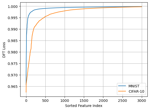
Fig. 1: Illustration of the DFT curves for MNIST and CIFAR-10, where the y-axis indicates the loss function and the x-axis denotes the sorted representation index.

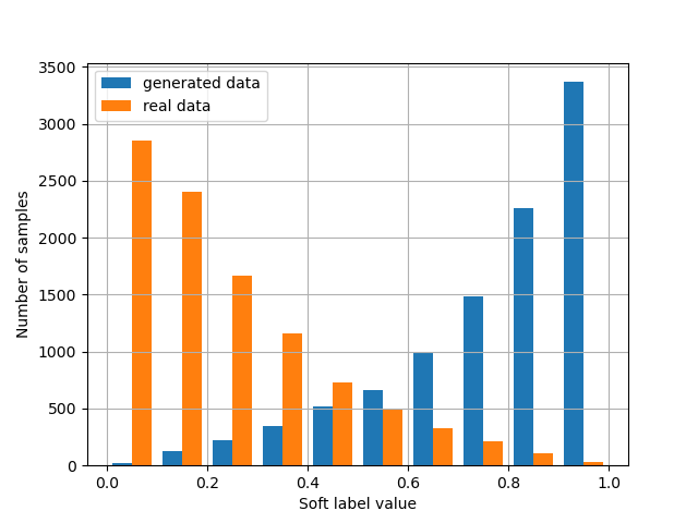
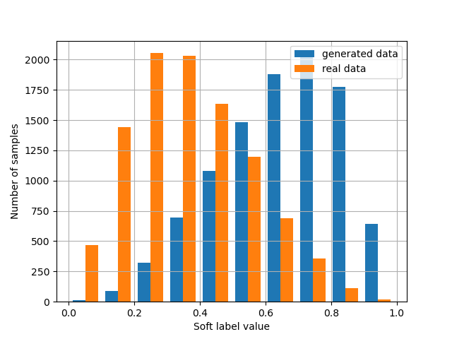
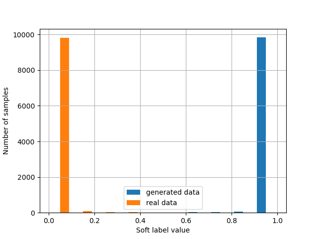
(a)                                                     (b)                                                     (c)

Fig. 2: The soft score histograms with generator models “Diffusion StyleGAN2” and “Styleformer” for CIFAR-10 are shown in (a) and (b), respectively, and the soft score histogram with generator model “WGAN-GP” for MNIST is shown in (c).

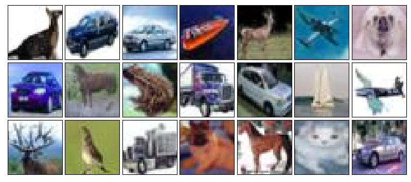
(a)

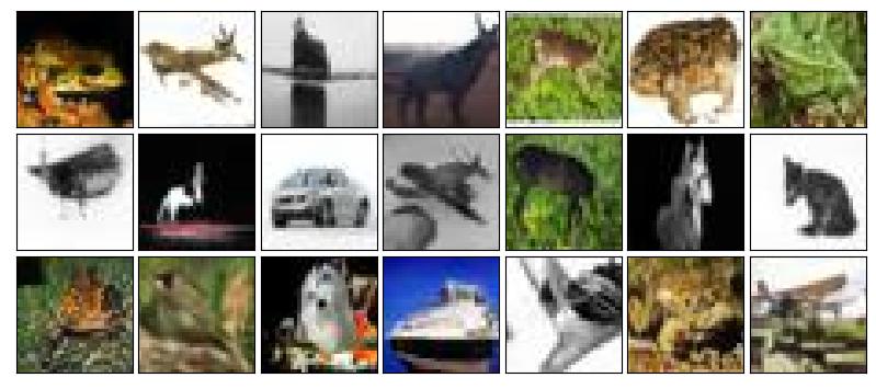
(b)

Fig. 3: Visualization of generated CIFAR-10 samples where samples of quality index close to 0 and 1 are shown in (a) and (b), respectively.

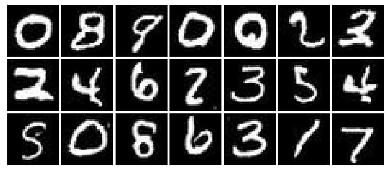
(a)

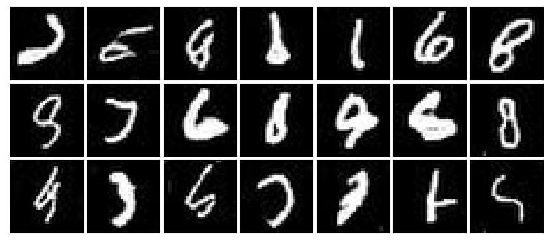
(b)

Fig. 4: Visualization of generated MNIST samples where samples of quality index close to 0 and 1 are shown in (a) and (b), respectively.

Module 2: Discriminant Feature Test (DFT)

The number of representations obtained from Module 1 is large. We need a mechanism to choose powerful ones against a particular task. This is achieved by the discriminant feature test (DFT) [21]. DFT analyzes the discriminant power of each representation based on the following idea. For the $i^{th}$ representation, it computes its value range, $[f^{i}_{min},f^{i}_{max}]$, and partition the range into two non-overlapping subsets, denoted by $S^{i}_{L}$ and $S^{i}_{R}$, with a set of uniformly-spaced partition points. The DFT loss is defined as the smallest weighted entropy of $S^{i}_{L}$ and $S^{i}_{R}$ in left and right partitions at the optimal partition point. Mathematically, it can be written as

$$L_{DFT}=\mathop{\min}_{t\in T}H_{t}^{i}=-\mathop{\min}_{t\in T}\sum^{C}_{c=1}[p^{i}_{L,c}\log(p^{i}_{L,c})+p^{i}_{R,c}\log(p^{i}_{R,c})]$$ (1)

Where $T$ denotes the set of uniformly-spaced partition points, $C$ is the class number and $p^{i}_{L,c}$ and $p^{i}_{R,c}$ denote the probability of the $i^{th}$ representation dimension being in class $c$ of the left or right interval, respectively.

The DFT loss can be computed for all representations in parallel since they are independent. The lower the DFT loss, the more discriminant of the representation dimension. The representations are sorted by their DFT loss in ascending order to yield the DFT loss curve as shown in Fig. 1. We can use the elbow point to select a subset of representations with lower DFT loss. They define a set of discriminant features to be fed into a binary classifier in Module 3.

Module 3: Binary Classification for Evaluation

We partition the real/generated data into training and testing sets. A binary classifier is trained on the union of real and generated training samples. They are labeled with “0” and “1”, respectively. The classifier assigns a soft score, $0\leq d\leq 1$, to each testing sample as the sample quality index. The hard decision depends on threshold $t$, where $0\leq t\leq 1$. The sample is labeled as “real” if $0\leq d<t$, and “generated” if $t\leq d\leq 1$. Four commonly used performance metrics of a binary classifier are reviewed below. They are accuracy (Acc.), precision (Pre.), recall (Rec.) and area under the curve (AUC). Accuracy is the ratio of the “correct decision number” over the “total decision number”. Precision and Recall is defined as

$$\mbox{Pre}=\frac{TP}{TP+FP},\quad\mbox{Rec}=\frac{TP}{TP+FN},$$ (2)

where, $TP$, $FP$, $TN$ and $FN$ indicate true positive, false positive, true negative, and false negative, respectively. AUC is computed by the precision-recall curve by varying threshold $t$ from zero to one.

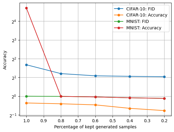
Fig. 5: Post-processing result.

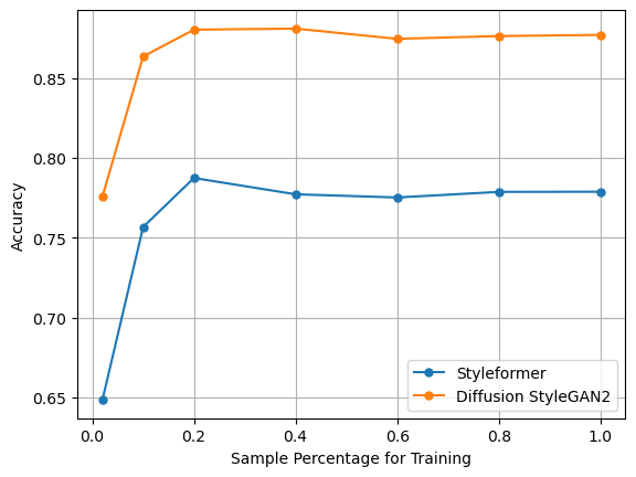
Fig. 6: The correct classification rates of LGSQE for samples generated by two models as a function of the number of real samples (expressed in terms of percentages of the total training samples).

4 Experiments

To show the effectiveness of the LGSQE method, we conduct experiments on the CIFAR-10 dataset, which is one of the most popular datasets in the image generation field. Multiple generative models such as DCGAN [22], StyleFormer [23], StyleGAN2-ADA [24], Diffusion-StyleGAN2 [25], and StyleGANXL [26] have been developed for this dataset. We also employ the MNIST dataset [27] in the experiment with three generative models; namely, GAN [28], WGAN [29] and WGAN-GP [30]. The hyperparameters in Module 1 are $F=3$, $S=1$ and $C=3$ for CIFAR-10 and $F=5$, $S=2$ and $C=1$ for MNIST. After discarding Saab coefficients of extremely low energy, 3,500 representations remain and DFT is conducted to get 800 most discriminant features for CIFAR-10. Similarly, 3,000 representations remain and 400 most discriminant features are kept for MNIST in Module 2. Finally, the XGBoost (extreme gradient boosting) classifier [31] is adopted in Module 3 as it has high performance with a small model size.

Evaluation of generated samples. A soft score (the probability of a sample belonging to class “one”) is assigned to each generated sample as a quality index by LGSQE. If a generated sample has a score close to one, it is likely to be a generated one. In contrast, a soft score closer to zero indicates a higher likelihood of being a real one. We show histograms of soft scores for real and generated samples computed by LGSQE for CIFAR-10, where the generator models in Fig. 2 (a) and (b) are Diffusion StyleGAN2 and Styleformer, respectively. By comparing these two histograms, we claim that Styleformer is a better generator model than Diffusion StyleGAN2, since its generated samples and real ones are clustered in the middle region of soft score 0.5. They are more difficult to distinguish. The soft score histogram of WGAN-GP for MNIST is shown in Fig. 2 (c). Diffusion StyleGAN2 for CIFAR-10 and WGAN-GP for MNIST are both poor generators since their generated samples can be easily differentiated from real ones. To further demonstrate the power of the quality index, we show CIFAR-10 and MNIST generated examples with soft scores close to 0 and 1 for visual comparison in Figs. 3 and 4, respectively. Clearly, the soft score of a generated sample is correlated well with its visual quality viewed by humans.

Post-processing of generative models. This method can be applied as a post-processing procedure for improving the quality of generated samples by filtering out generated samples of bad quality. Generated samples are sorted by their soft scores in ascending order and good samples with smaller soft scores are kept as the post-processing result. Fig. 5 shows the accuracy and FID scores with different percentages of kept generated samples. To keep the same number of samples in accuracy and FID computation, more samples are used for filtering out bad samples when the kept percentage is small. As the kept percentage becomes smaller, the kept samples are of higher quality and accuracy and the FID score improves.

Evaluation of generative models. LGSQE provides evaluation metrics for generative models by aggregating the quality indices of a number of generative samples. For a generative model of good performance, the real and generated samples will have a larger overlap distribution region and thus more samples would have soft scores closer to 0.5. Thus, an accuracy closer to 0.5 indicates a better generative model. Table 1 compares the performance metrics of several methods in generative models evaluation, including (a) DCGAN, (b) Diffusion-StyleGAN2 (c) StyleGAN2-ADA, (d) Styleformer, and (e) StyleGAN-XL for CIFAR-10 (denoted by C) and (f) GAN, (g) WGAN, and (h) WGAN-GP for MNIST (denoted by M). Acc. (accuracy), AUC (area under the curve), Pre. (precision) and Rec. (recall) are results of the proposed method. AP (average precision) is the AUC of the precision-recall [6] curve, in which the precision and recall are defined as quality and diversity metrics and a higher AP means a better generative model. The performance ranking of the proposed method is consistent with the most popular evaluation metric, FID, and this further corroborates the effectiveness of our method. Since AUC, Pre. and Rec. are close to AUC, these values aren’t computed for MNIST.

Table 1: Performance comparison of several evaluation metrics.

DS.	Model	FID	IS	AP	Acc.	AUC	Pre.	Rec.
C	(a)	47.7	6.58	0.86	0.95	0.99	0.95	0.95
	(b)	3.19	-	0.87	0.88	0.95	0.88	0.88
	(c)	2.92	9.83	0.87	0.84	0.92	0.84	0.84
	(d)	2.82	9.94	0.83	0.776	0.86	0.77	0.78
	(e)	1.85	-	0.79	0.62	0.68	0.62	0.65
M	(f)	26.56	-	0.72	0.99	-	-	-
	(g)	32.37	-	0.58	0.99	-	-	-
	(h)	26.12	-	0.65	0.76	-	-	-

High model efficiency. LGSQE has higher efficiency in terms of its model size and inference time compared with other quality evaluation metrics. The state-of-the-art metrics extract features from Inception-v3, VGG-16, or ResNet-34 pretrained on ImageNet. Their model sizes are 91.2MB, 138.4MB, and 83MB, respectively. However, it only takes 2-3 MB of memory for LGSQE to finish the whole evaluation process, including training and testing. It takes 122 minutes to finish FID computation on 10,000 pairs of generated and real images, while LGSQE only needs 2 to 3 minutes to complete the test under the same computing setting.

Setting of weakly supervised learning. LGSQE can achieve similar evaluation performance even with a smaller number of training samples. We show the test accuracy of LGSQE for CIFAR-10 as a function of the number of training samples in Fig. 6 with two generative models (i.e., Styleformer and Diffusion-StyleGAN). The accuracy converges when 20% real samples are used in training. In contrast, FID and other evaluation metrics apply complex networks to extract features. They demand more training data to get accurate distribution statistics for the evaluation purpose.

5 Conclusion and Future Work

A lightweight evaluation metric, LGSQE, was presented to evaluate the quality index of a generated sample. To the best of our knowledge, this is the first quality metric developed for such a purpose. It can also be employed as an evaluation metric for generative models, maintaining the same performance as other metrics, yet demanding fewer model parameters, fewer training samples, and less inference time. LGSQE can be potentially used as a post-processing module for high quality image generation. That is, it can reject low quality samples and, thus, improve the overall image generation performance. This is an interesting topic for future exploration.

References

- [1] A. Borji, “Pros and cons of gan evaluation measures,” Computer Vision and Image Understanding, vol. 179, pp. 41–65, 2019.
- [2] ——, “Pros and cons of gan evaluation measures: New developments,” Computer Vision and Image Understanding, vol. 215, p. 103329, 2022.
- [3] T. Salimans, I. Goodfellow, W. Zaremba, V. Cheung, A. Radford, and X. Chen, “Improved techniques for training gans,” Advances in neural information processing systems, vol. 29, 2016.
- [4] M. Heusel, H. Ramsauer, T. Unterthiner, B. Nessler, and S. Hochreiter, “Gans trained by a two time-scale update rule converge to a local nash equilibrium,” Advances in neural information processing systems, vol. 30, 2017.
- [5] D. Lopez-Paz and M. Oquab, “Revisiting classifier two-sample tests,” arXiv preprint arXiv:1610.06545, 2016.
- [6] M. S. Sajjadi, O. Bachem, M. Lucic, O. Bousquet, and S. Gelly, “Assessing generative models via precision and recall,” Advances in neural information processing systems, vol. 31, 2018.
- [7] A. Alaa, B. Van Breugel, E. S. Saveliev, and M. van der Schaar, “How faithful is your synthetic data? sample-level metrics for evaluating and auditing generative models,” in International Conference on Machine Learning. PMLR, 2022, pp. 290–306.
- [8] D. J. Im, H. Ma, G. Taylor, and K. Branson, “Quantitatively evaluating gans with divergences proposed for training,” arXiv preprint arXiv:1803.01045, 2018.
- [9] M. F. Naeem, S. J. Oh, Y. Uh, Y. Choi, and J. Yoo, “Reliable fidelity and diversity metrics for generative models,” in International Conference on Machine Learning. PMLR, 2020, pp. 7176–7185.
- [10] J. Yang, A. Kannan, D. Batra, and D. Parikh, “Lr-gan: Layered recursive generative adversarial networks for image generation,” arXiv preprint arXiv:1703.01560, 2017.
- [11] L. Theis, A. v. d. Oord, and M. Bethge, “A note on the evaluation of generative models,” arXiv preprint arXiv:1511.01844, 2015.
- [12] S. Liu, Y. Wei, J. Lu, and J. Zhou, “An improved evaluation framework for generative adversarial networks,” arXiv preprint arXiv:1803.07474, 2018.
- [13] M. Lucic, K. Kurach, M. Michalski, S. Gelly, and O. Bousquet, “Are gans created equal? a large-scale study,” Advances in neural information processing systems, vol. 31, 2018.
- [14] C.-C. J. Kuo and A. M. Madni, “Green learning: Introduction, examples and outlook,” arXiv preprint arXiv:2210.00965, 2022.
- [15] C.-C. J. Kuo, “Understanding convolutional neural networks with a mathematical model,” Journal of Visual Communication and Image Representation, vol. 41, pp. 406–413, 2016.
- [16] ——, “The cnn as a guided multilayer recos transform [lecture notes],” IEEE signal processing magazine, vol. 34, no. 3, pp. 81–89, 2017.
- [17] C.-C. J. Kuo, M. Zhang, S. Li, J. Duan, and Y. Chen, “Interpretable convolutional neural networks via feedforward design,” Journal of Visual Communication and Image Representation, vol. 60, pp. 346–359, 2019.
- [18] Y. Chen and C.-C. J. Kuo, “Pixelhop: A successive subspace learning (SSL) method for object recognition,” Journal of Visual Communication and Image Representation, p. 102749, 2020.
- [19] Y. Chen, M. Rouhsedaghat, S. You, R. Rao, and C.-C. J. Kuo, “Pixelhop++: A small successive-subspace-learning-based (ssl-based) model for image classification,” in 2020 IEEE International Conference on Image Processing (ICIP). IEEE, 2020, pp. 3294–3298.
- [20] Y. Yang, H. Fu, and C.-C. J. Kuo, “Design of supervision-scalable learning systems: Methodology and performance benchmarking,” arXiv e-prints, pp. arXiv–2206, 2022.
- [21] Y. Yang, W. Wang, H. Fu, and C.-C. J. Kuo, “On supervised feature selection from high dimensional feature spaces,” arXiv preprint arXiv:2203.11924, 2022.
- [22] A. Radford, L. Metz, and S. Chintala, “Unsupervised representation learning with deep convolutional generative adversarial networks,” arXiv preprint arXiv:1511.06434, 2015.
- [23] J. Park and Y. Kim, “Styleformer: Transformer based generative adversarial networks with style vector,” in Proceedings of the IEEE/CVF Conference on Computer Vision and Pattern Recognition, 2022, pp. 8983–8992.
- [24] T. Karras, M. Aittala, J. Hellsten, S. Laine, J. Lehtinen, and T. Aila, “Training generative adversarial networks with limited data,” Advances in Neural Information Processing Systems, vol. 33, pp. 12 104–12 114, 2020.
- [25] Z. Wang, H. Zheng, P. He, W. Chen, and M. Zhou, “Diffusion-gan: Training gans with diffusion,” arXiv preprint arXiv:2206.02262, 2022.
- [26] A. Sauer, K. Schwarz, and A. Geiger, “Stylegan-xl: Scaling stylegan to large diverse datasets,” in Special Interest Group on Computer Graphics and Interactive Techniques Conference Proceedings, 2022, pp. 1–10.
- [27] Y. LeCun, L. Bottou, Y. Bengio, and P. Haffner, “Gradient-based learning applied to document recognition,” Proceedings of the IEEE, vol. 86, no. 11, pp. 2278–2324, 1998.
- [28] I. Goodfellow, J. Pouget-Abadie, M. Mirza, B. Xu, D. Warde-Farley, S. Ozair, A. Courville, and Y. Bengio, “Generative adversarial nets,” Advances in neural information processing systems, vol. 27, 2014.
- [29] M. Arjovsky, S. Chintala, and L. Bottou, “Wasserstein generative adversarial networks,” in International conference on machine learning. PMLR, 2017, pp. 214–223.
- [30] I. Gulrajani, F. Ahmed, M. Arjovsky, V. Dumoulin, and A. C. Courville, “Improved training of wasserstein gans,” Advances in neural information processing systems, vol. 30, 2017.
- [31] T. Chen and C. Guestrin, “Xgboost: A scalable tree boosting system,” in Proceedings of the 22nd acm sigkdd international conference on knowledge discovery and data mining, 2016, pp. 785–794.