Quantum triangles and imaginary geometry flow lines

Abstract

We define a three-parameter family of random surfaces in Liouville quantum gravity (LQG) which can be viewed as the quantum version of triangles. These quantum triangles are natural in two senses. First, by our definition they produce the boundary three-point correlation functions of Liouville conformal field theory on the disk. Second, it turns out that the laws of the triangles bounded by flow lines in imaginary geometry coupled with LQG are given by these quantum triangles. In this paper we demonstrate the second point for boundary flow lines on a quantum disk. Our method has the potential to prove general conformal welding results with quantum triangles glued in an arbitrary way. Quantum triangles play a basic role in understanding the integrability of SLE and LQG via conformal welding. In this paper, we deduce integrability results for chordal SLE with three force points, using the conformal welding of a quantum triangle and a two-pointed quantum disk. Further applications will be explored in subsequent works.

1 Introduction

Schramm-Loewner evolution (SLE) and Liouville quantum gravity (LQG) are central subjects in random conformal geometry as canonical theories for random curves and surfaces, respectively. Starting from [She16], a key tool to study SLE and LQG is their coupling, where SLE curves arise as the interfaces of LQG surfaces under conformal welding. This leads to the mating-of-trees theory [DMS21], which is fundamental in connecting LQG and the scaling limits of random planar maps decorated with statistical physics models; see the textbook [BP21] and the survey [GHS19]. More recently, conformal welding was used to study the integrability of SLE and LQG [AHS21, ARS21, AS21].

In most conformal welding results established so far, the SLE curves cut the LQG surfaces into smaller surfaces with two boundary marked points. The infinite-area version of these two-pointed marked surfaces are called quantum wedges, while the finite-area variants are called two-pointed quantum disks. As shown in [DMS21, AHS20], when these surfaces are welded together, the law of the SLE interfaces are a collection of flow lines in the sense of imaginary geometry [MS16a, MS17], which is a canonical framework to couple multiple SLE curves. Two-pointed quantum disks also plays a basic role in the Liouville conformal field theory (LCFT) as they determine the reflection coefficient for LCFT on the disk [HRV18, RZ22, AHS21].

In this paper we define a three-parameter family of LQG surfaces with three boundary marked points, which we call quantum triangles. They are defined to produce the boundary three-point correlation functions of LCFT on the disk. When two of the parameters are equal, they reduce to a two-parameter family of quantum surfaces defined in [AHS21]. The main goal of our paper is to demonstrate that the law of the triangular surfaces cut out by imaginary geometry flow lines on a LQG disk with multiple boundary marked points are given by quantum triangles; see Theorem 1.3. Based on our work, a general result with quantum triangles conformally welded in an arbitrary way will be proved by the first and the third authors in a subsequent work. Quantum triangles enrich the applications of conformal welding to SLE and LQG. In this paper, we deduce integrablity results for chordal SLE with three force points. Further applications will be discussed in Section 1.5.

We will give a brief description of quantum triangles in Section 1.1 with the precise definition postponed to Section 2. Then in Section 1.2 we state a key result (Theorem 1.2) saying that the conformal welding of a quantum triangle and a two-pointed quantum disk gives another quantum triangle, which is proved in Sections 4—6. The proof includes several novel techniques for proving general conformal welding results. In particular, we give a Markovian characterization of the Liouville fields defining quantum triangles, which explains their ubiquity. As a corollary of Theorem 1.2, we state the aforementioned Theorem 1.3 in Section 1.3 with more details on imaginary geometry provided in Section 3. We present some applications of Theorem 1.2 to SLE in Section 1.4, whose proofs are given in Section 7. In Section 1.5, we discuss some perspectives and related works.

1.1 Definition of the quantum triangle

Fix $\gamma\in(0,2)$. A quantum surface in $\gamma$-LQG is a surface with an area measure and a metric structure induced by a variant of Gaussian free field (GFF). The area is defined in [DS11] and the metric is defined in [DDDF20, GM21]. A quantum surface with the disk topology can be represented as a pair $(D,h)$ where $D$ is a simply connected domain and $h$ is a variant of GFF. For such surfaces there is also a notion of $\gamma$-LQG length measure on the disk boundary [DS11]. Two pairs $(D,h)$ and $(D^{\prime},h^{\prime})$ represent the same quantum surface if there is a conformal map between $D$ and $D^{\prime}$ preserving the geometry. A particular pair $(D,h)$ is called a (conformal) embedding of the quantum surface.

For $W>0$, the two-pointed quantum disk of weight $W$ is a quantum surface with two boundary marked points introduced in [DMS21, AHS20], which has finite quantum area and length. It has two regimes: thick (i.e. $W\geq\frac{\gamma^{2}}{2}$) and thin (i.e. $W\in(0,\frac{\gamma^{2}}{2})$). For $W\geq\gamma^{2}/2$, the two-pointed quantum disk has the disk topology with two boundary marked points. The field near the two marked points has a $\beta$-log singularity where $\beta$ and $W$ are related by

$$\beta=\gamma+\frac{2-W}{\gamma},\quad\textrm{i.e.}\quad W=\gamma(Q+\frac{\gamma}{2}-\beta).$$ (1.1)

For $W\in(0,\gamma^{2}/2)$, the weight-$W$ two-pointed quantum disk has the topology of an ordered collection of disks, each of which has two boundary marked points. There is a canonical law $\mathcal{M}_{2}^{\textup{disk}}(W)$ for the weight-$W$ two-pointed quantum disk, which has no constraint on the total area and boundary lengths. Other variants with fixed area and/or length can be obtained from $\mathcal{M}_{2}^{\textup{disk}}(W)$ by conditioning. We also write $\mathcal{M}_{2}^{\textup{disk}}(2)$ as $\mathrm{QD}_{0,2}$. A sample from $\mathrm{QD}_{0,2}$ is known as the quantum disk with two typical boundary points, because in this case the two marked points are simply distributed according to the $\gamma$-LQG boundary length measure. This special case arises naturally as scaling limits of random planar maps. For example, when $\gamma=\sqrt{8/3}$, $\mathrm{QD}_{0,2}$ is the law of the LQG realization of the Brownian disk with two boundary marked points, with free area and boundary length [MS20, MS21]. This is the scaling limit of triangulation or quadrangulations sampled from the critical Boltzmann measure [BM17, GM19]. In general, $\mathcal{M}_{2}^{\textup{disk}}(W)$ is an infinite measure. For $W\in(0,\frac{\gamma^{2}}{2})$, the ordered collections of disks in $\mathcal{M}_{2}^{\textup{disk}}(W)$ can be obtained from an initial segment of the Poisson point process with intensity measure $\mathcal{M}_{2}^{\textup{disk}}(\gamma^{2}-W)$. We will recall the precise definition of $\mathcal{M}_{2}^{\textup{disk}}(W)$ in Section 2.

Two-pointed quantum disks are intimately related to Liouville conformal field theory on the disk [HRV18]. This relation is most transparent when we parameterize a quantum disk by a strip. Let $\mathcal{S}$ be the horizontal strip $\mathbb{R}\times(0,\pi)$. For $W>\frac{\gamma^{2}}{2}$, let $(\mathcal{S},\phi,+\infty,-\infty)$ be an embedding of a sample from $\mathcal{M}_{2}^{\textup{disk}}(W)$. Let $\beta=\gamma+\frac{2-W}{\gamma}<Q$ as in (1.1). By [AHS21], if we independently sample $T$ from the Lebesgue measure on $\mathbb{R}$, then the law of the field $\tilde{\phi}:=\phi(\cdot+T)$ is $\frac{\gamma}{2(Q-\beta)^{2}}\textup{LF}_{\mathcal{S}}^{(\beta,\pm\infty)}$, where $\textup{LF}_{\mathcal{S}}^{(\beta,\pm\infty)}$ is the Liouville field on $\mathcal{S}$ with $\beta$ insertions at $\pm\infty$. See Section 2 for the definition of Liouville fields with insertions.

We now describe our main quantum surfaces of interest, the quantum triangles. We first recall a special case that is already considered in [AHS21] and played a crucial rule there. For $\beta,\beta_{3}<Q$, the Liouville field measure $\textup{LF}_{\mathcal{S}}^{(\beta,\pm\infty),(0,\beta_{3})}$ is formally defined by $\textup{LF}_{\mathcal{S}}^{(\beta,\pm\infty),(\beta_{3},0)}(d\phi)=e^{\beta_{3}\phi(0)}\textup{LF}_{\mathcal{S}}^{(\beta,\pm\infty)}(d\phi)$, and can be made rigorous by regularization. Let $W,W_{3}>\frac{\gamma^{2}}{2}$ be determined by $\beta,\beta_{3}$ as in (1.1), respectively. Sample $\phi$ from $\frac{1}{(Q-\beta)^{2}(Q-\beta_{3})}\textup{LF}_{\mathcal{S}}^{(\beta,\pm\infty),(0,\beta_{3})}$ and let $\mathrm{QT}(W,W,W_{3})$ be the law of the three-pointed quantum surface $(\mathcal{S},\phi,\pm\infty,0)$. We call a sample from $\mathrm{QT}(W,W,W_{3})$ a quantum triangle of weight $(W,W,W_{3})$. Up to a multiplicative constant, the measure $\mathrm{QT}(W,W,W_{3})$ agrees with $\mathcal{M}_{2,\bullet}^{\textup{disk}}(W;\beta_{3})$ defined in [AHS21]; also see Definition 2.15. For $W=\frac{\gamma^{2}}{2}$, we define $\mathrm{QT}(\frac{\gamma^{2}}{2},\frac{\gamma^{2}}{2},W_{3})$ as the $W\downarrow\frac{\gamma^{2}}{2}$ limit of $\mathrm{QT}(W,W,W_{3})$. For $W\in(0,\frac{\gamma^{2}}{2})$, following the definition of $\mathcal{M}_{2,\bullet}^{\textup{disk}}(W;\beta_{3})$ in [AHS21], we let $\mathrm{QT}(W,W,W_{3})$ be the law of the three-pointed surface obtained by attaching an independent weight-$W$ two pointed disk at a quantum triangle of weight $(\gamma^{2}-W,\gamma^{2}-W,W_{3})$.

For $W_{1},W_{2},W_{3}>0$, we define $\mathrm{QT}(W_{1},W_{2},W_{3})$ as follows. For $W_{1},W_{2},W_{3}>\frac{\gamma^{2}}{2}$, set $\beta_{i}=\gamma+\frac{2-W_{i}}{\gamma}<Q$ and let $\textup{LF}_{\mathcal{S}}^{(\beta_{1},+\infty),(\beta_{2},-\infty),(\beta_{3},0)}$ be the Liouville field on $\mathcal{S}$ with insertion $\beta_{1},\beta_{2},\beta_{3}$ at $+\infty,-\infty$ and $0$, respectively. Sample $\phi$ from

$$\frac{1}{(Q-\beta_{1})(Q-\beta_{2})(Q-\beta_{3})}\textup{LF}_{\mathcal{S}}^{(\beta_{1},+\infty),(\beta_{2},-\infty),(\beta_{3},0)}.$$

We define $\textup{QT}(W_{1},W_{2},W_{3})$ to be the law of the 3-pointed quantum surface $(\mathcal{S},\phi,+\infty,-\infty,0)$. We call a sample from $\mathrm{QT}(W,W,W_{3})$ a quantum triangle of weight $(W_{1},W_{2},W_{3})$. Taking the limit $W_{i}\downarrow\frac{\gamma^{2}}{2}$, we can extend the definition of $\textup{QT}(W_{1},W_{2},W_{3})$ to $W_{1},W_{2},W_{3}\geq\frac{\gamma^{2}}{2}$; see Section 2.5. In this regime a quantum triangle has the disk topology. When $W_{1}\in(0,\frac{\gamma^{2}}{2})$ and $W_{2},W_{3}\geq\frac{\gamma^{2}}{2}$, we define $\mathrm{QT}(W_{1},W_{2},W_{3})$ by attaching an independent weight-$W_{1}$ two pointed disk at a quantum triangle of weight $(\gamma^{2}-W_{1},W_{2},W_{3})$. Using this method we extend the definition of $\textup{QT}(W_{1},W_{2},W_{3})$ to $W_{1},W_{2},W_{3}>0$. We call the three marked points vertices of a quantum triangle and $W_{i}$ ($i=1,2,3$) is called the weight of the corresponding vertex. Given a sample of $\mathrm{QT}(W_{1},W_{2},W_{3})$, the geometry near the vertex of weight $W_{i}$ looks like the neighborhood of a marked point on a weight-$W_{i}$ quantum disk. We say a vertex is thick if its weight $W\geq\frac{\gamma^{2}}{2}$. We call it thin if $W\in(0,\frac{\gamma^{2}}{2})$. See Figure 1 for an illustration.

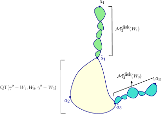
Figure 1: A sample of $\mathrm{QT}(W_{1},W_{2},W_{3})$ with a thick vertex $a_{2}$ and two thin vertices $a_{1},a_{3}$, i.e. $W_{2}\geq\frac{\gamma^{2}}{2}$ and $W_{1},W_{3}<\frac{\gamma^{2}}{2}$. The yellow surface is a quantum triangle with thick vertices $\tilde{a}_{1},a_{2},\tilde{a}_{3}$. The two thin two-pointed quantum disks (colored green) are concatenated with the yellow triangle at $\tilde{a}_{1}$ and $\tilde{a}_{3}$.

1.2 Conformal welding of a quantum triangle and a 2-pointed quantum disks

We first recall the conformal welding result for two-pointed quantum disk proved in [AHS20] based on its infinite-area variant in [DMS21]. For $W>0$, define $\mathcal{M}_{2}^{\textup{disk}}(W;\ell,r)$ via the disintegration $\mathcal{M}_{2}^{\textup{disk}}(W)=\iint_{0}^{\infty}\mathcal{M}_{2}^{\textup{disk}}(W;\ell,r)d\ell dr$, where $\mathcal{M}_{2}^{\textup{disk}}(W;\ell,r)$ is supported on surfaces with left boundary length $\ell$ and right boundary length $r$. Given a pair of quantum surfaces sampled from $\mathcal{M}_{2}^{\textup{disk}}(W_{1};\ell_{1},\ell)\times\mathcal{M}_{2}^{\textup{disk}}(W_{2};\ell,\ell_{2})$, we can conformally weld them together along the boundary with length $\ell$ to obtain a quantum surface decorated with a curve. We denote its law by $\mathrm{Weld}(\mathcal{M}_{2}^{\textup{disk}}(W_{1};\ell_{1},\ell),\mathcal{M}_{2}^{\textup{disk}}(W_{2};\ell,\ell_{2}))$. For $\kappa>0$, $\rho_{-}>-2$ and $\rho_{+}>-2$, chordal $\mathrm{SLE}_{\kappa}(\rho_{-};\rho_{+})$ is a classical variant of SLE_κ curve on simply connected domain between two boundary points, which will be recalled in Section 3.1. Fix $W_{1},W_{2}>0$, the conformal welding result for $\mathcal{M}_{2}^{\textup{disk}}(W_{1})$ and $\mathcal{M}_{2}^{\textup{disk}}(W_{2})$ says the following. Let $(D,h,a,b)$ be an embedding of a two-pointed quantum disk sampled from $\mathcal{M}_{2}^{\textup{disk}}(W_{1}+W_{2})$ with $a,b$ being the two boundary marked points. Let $\eta$ be a $\mathrm{SLE}_{\kappa}(\rho^{-};\rho^{+})$ curve on $D$ from $a$ to $b$ independent of $h$, where

$$\kappa=\gamma^{2}\in(0,4);\quad\textrm{and}\quad\rho_{-}=W_{1}-2>-2;\quad\textrm{and}\quad\rho_{+}=W_{2}-2>-2.$$ (1.2)

We write $\mathcal{M}_{2}^{\textup{disk}}(W_{1}+W_{2})\otimes{\mathrm{SLE}}_{\kappa}(W_{1}-2;W_{2}-2)$ as the law of the curve-decorated surface $(D,h,\eta,a,b)$. Then there is a constant $c>0$ such that

$$\mathcal{M}_{2}^{\textup{disk}}(W_{1}+W_{2})\otimes{\mathrm{SLE}}_{\kappa}(W_{1}-2;W_{2}-2)=c\textup{Weld}(\mathcal{M}_{2}^{\textup{disk}}(W_{1}),\mathcal{M}_{2}^{\textup{disk}}(W_{2})),$$ (1.3)

where $\textup{Weld}(\mathcal{M}_{2}^{\textup{disk}}(W_{1}),\mathcal{M}_{2}^{\textup{disk}}(W_{2})):=\iiint_{0}^{\infty}\textup{Weld}(\mathcal{M}_{2}^{\textup{disk}}(W_{1};\ell,\ell_{1}),\mathcal{M}_{2}^{\textup{disk}}(W_{2};\ell_{1},\ell_{2}))d\ell d\ell_{1}d\ell_{2}$ is called the conformal welding of $\mathcal{M}_{2}^{\textup{disk}}(W_{1})$ and $\mathcal{M}_{2}^{\textup{disk}}(W_{2})$.

The bulk of our paper is devoted to proving that the conformal welding of a quantum triangle and a two-pointed quantum disk gives another quantum triangle with an SLE curve whose law is explicit. Similarly as in (1.3), we define $\mathrm{QT}(W_{1},W_{2},W_{3};\ell_{1},\ell_{2},\ell_{3})$ via the disintegration $\mathrm{QT}(W_{1},W_{2},W_{3})=\int\mathrm{QT}(W_{1},W_{2},W_{3};\ell_{1},\ell_{2},\ell_{3})d\ell_{1}d\ell_{2}d\ell_{3}$. Here $\ell_{i}$ is the length between the weight-$W_{i}$ and weight-$W_{i+1}$ vertices where $i=1,2,3$ and $3+1$ is identified with $1$. Fix $W,W_{1},W_{2},W_{3}>0$, given a pair of quantum surfaces sampled from $\mathcal{M}_{2}^{\textup{disk}}(W;\ell_{1},\ell)\times\mathrm{QT}(W_{1},W_{2},W_{3};\ell,\ell_{2},\ell_{3})$, we conformally weld them together along the boundary with length $\ell$ to obtain a quantum surface decorated with a curve and three marked points, whose law is denoted by $\mathrm{Weld}(\mathcal{M}_{2}^{\textup{disk}}(W;\ell,\ell_{1}),\mathrm{QT}(W_{1},W_{2},W_{3};\ell,\ell_{2},\ell_{3}))$. We define the conformal welding of $\mathcal{M}_{2}^{\textup{disk}}(W)$ and $\mathrm{QT}(W_{1},W_{2},W_{3})$ by

$$\textup{Weld}(\mathcal{M}_{2}^{\textup{disk}}(W),\mathrm{QT}(W_{1},W_{2},W_{3})):=\iiiint_{0}^{\infty}\mathrm{Weld}({\mathcal{M}}^{\mathrm{disk}}_{2}(W;\ell_{1},\ell),\mathrm{QT}(W_{1},W_{2},W_{3};\ell,\ell_{2},\ell_{3}))d\ell d\ell_{1}d\ell_{2}d\ell_{3}.$$ (1.4)

Similar to (1.3), the law of the three pointed quantum surface for $\textup{Weld}(\mathcal{M}_{2}^{\textup{disk}}(W),\mathrm{QT}(W_{1},W_{2},W_{3}))$ is proportional to $\mathrm{QT}(W+W_{1},W+W_{2},W_{3})$. To describe the law of the SLE interface, we need chordal $\mathrm{SLE}_{\kappa}$ with multiple boundary forces points, which is a more general variant of chordal $\mathrm{SLE}$ that arises in imaginary geometry [MS16a]. We let $\mathrm{SLE}_{\kappa}(\rho_{-};\rho_{+},\rho_{1})$ be the law of a chordal $\mathrm{SLE}_{\kappa}$ on the upper half plane $\mathbb{H}$ from $0$ to $\infty$ with forces points at $0^{-},0^{+},1$, whose weight are $\rho_{-},\rho_{+},\rho_{1}$ respectively. We will recall its definition in Section 3, for now it is sufficient to know that it is a random simple curve on $\mathbb{H}$ from $0$ to $\infty$, with an additional boundary marked points $0^{-},0^{+},1$ called force points, each of which is labeled by a number called weight. (This is not to be confused with the weight for a vertex of a quantum triangle). Our previous notion of chordal $\mathrm{SLE}_{\kappa}(\rho_{-};\rho_{+})$ on $\mathbb{H}$ from $0$ to $\infty$ is the special case where $\rho_{1}=0$.

Our first welding result (Theorem 1.1) says that when $W_{1},W_{2},W_{3}$ satisfies $W_{1}+2=W_{2}+W_{3}$, the interface in $\textup{Weld}(\mathcal{M}_{2}^{\textup{disk}}(W),\mathrm{QT}(W_{1},W_{2},W_{3}))$ is a chordal $\mathrm{SLE}_{\kappa}(W-2;W_{2}-2,W_{1}-W_{2})$ curve if $W+W_{1},W+W_{2},W_{3}$ are all thick weights (namely $\geq\frac{\gamma^{2}}{2}$); and if some of $W+W_{1},W+W_{2},W_{3}$ are thin, the analogous result holds after natural modifications. Let us first assume $W+W_{1},W+W_{2},W_{3}$ are all thick so that a sample from $\mathrm{QT}(W+W_{1},W+W_{2},W_{3})$ can be embedded as $(\mathbb{H},h,0,\infty,1)$. Sample $\eta$ from ${\mathrm{SLE}}_{\kappa}(W-2;W_{2}-2,W_{1}-W_{2})$ independently from $h$. We write $\mathrm{QT}(W+W_{1},W+W_{2},W_{3})\otimes{\mathrm{SLE}}_{\kappa}(W-2;W_{2}-2,W_{1}-W_{2})$ as the law of the curve-decorated surface $(\mathbb{H},h,\eta,0,\infty,1)$. Now if $W_{3}\in(0,\frac{\gamma^{2}}{2})$ instead, then a sample of $\mathrm{QT}(W+W_{1},W+W_{2},W_{3})$ can be obtained by attaching a weight $W_{3}$ two-pointed quantum disk to a quantum triangle of weight $(W+W_{1},W+W_{2},\gamma^{2}-W_{3})$ at the weight $(\gamma^{2}-W_{3})$ vertex. We now embed the weight $(W+W_{1},W+W_{2},\gamma^{2}-W_{3})$ triangle to $(\mathbb{H},0,+\infty,1)$ and run an independent ${\mathrm{SLE}}_{\kappa}(W-2;W_{2}-2,W_{1}-W_{2})$ curve from $0$ to $\infty$. We still write $\mathrm{QT}(W+W_{1},W+W_{2},W_{3})\otimes{\mathrm{SLE}}_{\kappa}(W-2;W_{2}-2,W_{1}-W_{2})$ as the law of the resulting curve-decorated surface with the two-pointed quantum disk attached. We will give the precise definition of this law for the case when $W+W_{1}$ or $W+W_{2}$ is thin in Section 6. See Figure 2 for illustrations of various cases.

Theorem 1.1.

Suppose $W,W_{1},W_{2},W_{3}>0$ with $W_{1}+2=W_{2}+W_{3}$. Then there exists some constant $c=c_{W,W_{1},W_{2}}\in(0,\infty)$ such that

$$\mathrm{QT}(W+W_{1},W+W_{2},W_{3})\otimes{\mathrm{SLE}}_{\kappa}(W-2;W_{2}-2,W_{1}-W_{2})=c\textup{Weld}(\mathcal{M}_{2}^{\textup{disk}}(W),\mathrm{QT}(W_{1},W_{2},W_{3})).$$ (1.5)

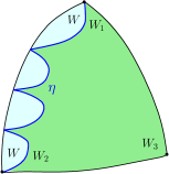
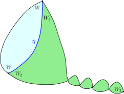
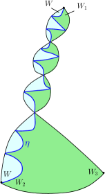
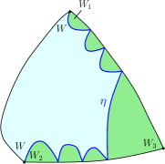
Figure 2: Illustration of some topological scenarios in Theorem 1.1. (a) $W\in(0,\frac{\gamma^{2}}{2})$ and $W_{1},W_{2},W_{3}\geq\frac{\gamma^{2}}{2}$; (b) $W,W_{1},W_{2}\geq\frac{\gamma^{2}}{2}$ and $W_{3}\in(0,\frac{\gamma^{2}}{2})$; (c) $W+W_{1}\in(0,\frac{\gamma^{2}}{2})$ and $W_{2},W_{3}\geq\frac{\gamma^{2}}{2}$; (d) $W,W_{3}\geq\frac{\gamma^{2}}{2}$ and $W_{1},W_{2}\in(0,\frac{\gamma^{2}}{2})$.

As we will see in Theorem 1.3, quantum triangles whose weight satisfy $W_{1}-W_{2}=W_{3}-2$ are those that will appear naturally in imaginary geometry on quantum disk with boundary typical points. The conformal welding result for $W_{1}-W_{2}\neq W_{3}-2$ can be easily deduced from Theorem 1.1 following arguments in [AHS21]. Suppose $\eta$ is a curve from 0 to $\infty$ on $\mathbb{H}$ that does not touch $1$. Let $D_{\eta}$ be the component of $\mathbb{H}\backslash\eta$ containing $1$, and $\psi_{\eta}$ is the unique conformal map from the component $D_{\eta}$ to $\mathbb{H}$ fixing 1 and sending the first (resp. last) point on $\partial D_{\eta}$ hit by $\eta$ to 0 (resp. $\infty$). Define the measure $\widetilde{\mathrm{SLE}}_{\kappa}(\rho_{-};\rho_{+},\rho_{1};\alpha)$ on curves from 0 to $\infty$ on $\mathbb{H}$ as follows.

$$\frac{d\widetilde{\mathrm{SLE}}_{\kappa}(\rho_{-};\rho_{+},\rho_{1};\alpha)}{d{\mathrm{SLE}}_{\kappa}(\rho_{-};\rho_{+},\rho_{1})}(\eta)=\psi^{\prime}_{\eta}(1)^{\alpha}.$$ (1.6)

Then we have the following extension of Theorem 1.1.

Theorem 1.2.

Suppose $W,W_{1},W_{2},W_{3}>0$. Set

$$\alpha=\frac{W_{3}+W_{2}-W_{1}-2}{4\kappa}(W_{3}+W_{1}+2-W_{2}-\kappa).$$ (1.7)

Then with the same constant $c=c_{W,W_{1},W_{2}}\in(0,\infty)$ as in Theorem 1.1, we have

$$\mathrm{QT}(W+W_{1},W+W_{2},W_{3})\otimes\widetilde{\mathrm{SLE}}_{\kappa}(W-2;W_{2}-2,W_{1}-W_{2};\alpha)=c\textup{Weld}(\mathcal{M}_{2}^{\textup{disk}}(W),\mathrm{QT}(W_{1},W_{2},W_{3})).$$ (1.8)

We will give the precise definition of $\mathrm{QT}(W+W_{1},W+W_{2},W_{3})\otimes\widetilde{\mathrm{SLE}}_{\kappa}(W-2;W_{2}-2,W_{1}-W_{2};\alpha)$ in Section 6, which again requires a proper interpretation when some of $W+W_{1},W+W_{2},W_{3}$ are thin.

The proof of Theorems 1.1 and 1.2 is divided into three steps that are carried out in Sections 4—6, respectively. The first step (Theorem 4.1) intuitively says the following. Suppose $W_{1}>\gamma^{2}/2$ and $W_{2}\in(0,\gamma^{2}/2)$ in the welding equation (1.3) for $\mathcal{M}_{2}^{\textup{disk}}(W_{1})$ and $\mathcal{M}_{2}^{\textup{disk}}(W_{2})$, if a cut point is added to the weight-$W_{2}$ disk so that it is split into two independent copies of $\mathcal{M}_{2}^{\textup{disk}}(W_{2})$, then the addition of the third point create a quantum triangles with weights compatible with Theorem 1.2. Theorem 4.1 is proved via a limiting procedure based on results from [AHS21]. Quantum triangles that we are able to identify in this step all have two vertices of equal weight.

The second and third steps require essential new techniques for proving welding results. First of all, there is no existing mechanism to identify the law of a quantum surface obtained from welding that has three boundary marked points of three different log singularities. In Step 2 (Section 5), we provide a Markovian characterizations of the three-pointed Liouville field that allows us to identify the law of quantum triangles after welding $\mathcal{M}_{2}^{\textup{disk}}(W)$ and $\mathrm{QT}(W_{1},W_{2},W_{3})$ as in Theorem 1.1. This proves Theorems 1.1 and 1.2 in a restricted range of weights. The range constraint is removed in Step 3 (Section 6). For this purpose it is crucial to work under the setting of Theorem 1.2, because we need the freedom to perform conformal welding along different edges of the same quantum triangle where the condition $W_{1}+2=W_{2}+W_{3}$ in Theorem 1.1 cannot be satisfied simultaneously for every welding. Techniques in Sections 5 and 6 are quite robust and will play a crucial role in the subsequent work [AY] proving more general welding results for quantum triangles; see Section 1.5.

1.3 Imaginary geometry on a quantum disk with multiple boundary points

When welding multiple two-pointed quantum disks, the interfaces are a set of flow lines in imaginary geometry. We briefly recall the flow line construction from [MS16a]. For $\kappa\in(0,4)$ and $\rho_{-},\rho_{+}>-2$, set

$$\chi=\frac{2}{\sqrt{\kappa}}-\frac{\sqrt{\kappa}}{2}\quad\textrm{and}\quad\lambda=\frac{\pi}{\sqrt{\kappa}};\quad\quad\quad\lambda_{-}=-\lambda(1+\rho_{-})\quad\textrm{and}\quad\lambda_{+}=\lambda(1+\rho_{+}).$$ (1.9)

Let $\mathfrak{h}$ be a GFF on the upper half plane $\mathbb{H}$ with Dirichlet boundary condition such that the boundary value is $\lambda_{-}$ between $(-\infty,0)$ and $\lambda_{+}$ between $(0,\infty)$. Then there exists a coupling between $\mathfrak{h}$ and an $\mathrm{SLE}_{\kappa}(\rho_{-};\rho_{+})$ curve $\eta$ on $\mathbb{H}$ from 0 to $\infty$, under which $\eta$ is determined by $\mathfrak{h}$. Although $\mathfrak{h}$ is only a generalized function, the curve $\eta$ can be interpreted as the flow line from 0 to $\infty$ of the random vector field $e^{\frac{i\mathfrak{h}}{\chi}}$. For $\theta\in(-\frac{\lambda+\lambda_{+}}{\chi},\frac{\lambda-\lambda_{-}}{\chi})$, we can also consider the flow line of $e^{\frac{i\mathfrak{h}}{\chi}+\theta}$ which is the chordal $\mathrm{SLE}_{\kappa}(-\frac{\lambda_{-}+\chi\theta}{\lambda}-1;\frac{\lambda_{+}+\chi\theta}{\lambda}-1)$ determined by $\mathfrak{h}+\chi\theta$ via (1.9) with $(\lambda_{-},\lambda_{+})$ replaced by $(\lambda_{-}+\chi\theta,\lambda_{+}+\chi\theta)$. Varying $\theta$, we have multiple SLE curves between $0$ and $\infty$ with force points at $0^{-}$ and $0^{+}$coupled together. As generalization of (1.3), the conformal welding result from [AHS20] for multiple two-pointed quantum disks can be stated as follows. Fix $\gamma\in(0,2)$ and $\kappa=\gamma^{2}$. Consider $W=\sum_{i=0}^{n}W_{i}$ with $W_{i}>0$. Let $(\mathbb{H},h,0,\infty)$ be an embedding of a sample from $\mathcal{M}^{\mathrm{disk}}_{2}(W)$. Let $\mathfrak{h}$ be a GFF with boundary condition $\lambda_{-}=-(W-2)\lambda$ and $\lambda_{+}=0$. Let $\theta_{1}>\theta_{2}>\cdots>\theta_{n}$ be defined by

$$W_{i}=\frac{(\theta_{i}-\theta_{i+1})}{\lambda}\quad\textrm{for }i<n\quad\textrm{and}\quad W_{n}=1+\frac{\theta_{n}\chi}{\lambda}.$$ (1.10)

For $1\leq i\leq n$, let $\eta_{i}$ be the flow line of $e^{\frac{i\mathfrak{h}}{\chi}+\theta_{i}}$ from $0$ to $\infty$. Then the law of the decorated quantum surface $(\mathbb{H},h,\eta_{1},\cdots,\eta_{n})$ is given by the conformal welding of $\mathcal{M}_{2}^{\textup{disk}}(W_{1}),\cdots,\mathcal{M}_{2}^{\textup{disk}}(W_{n})$ in that order.

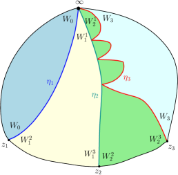
Figure 3: An illustration of Theorem 1.3 where $n=3$. The three flow lines cut the quantum disk $\mathrm{QD}_{0,4}$ into four parts: a weight $W_{0}$ and a weight $W_{3}$ quantum disk, a weight $(W^{1}_{1},W_{1}^{2},W_{1}^{3})$ thick quantum triange and a weight $(W_{2}^{1},W_{2}^{2},W_{2}^{3})$ thin triangle.

In the framework of imaginary geometry in [MS16a], it is possible to emanate flow lines from different boundary points with the same target point. Unfortunately the conformal welding result for two-pointed disk falls short of producing this rich picture. Thanks to the introduction of quantum triangles, this can now be achieved as in Theorem 1.3. Although our result can be stated more generally, we restrict ourselves to the following neat setting to make the point. We consider a quantum disk with more than two typical boundary marked points. For $n\geq 2$, a quantum disk with $n+1$ quantum typical can sampled as follows. First sample a two-pointed quantum disk from the tilted measure $L^{n-1}\mathrm{QD}_{0,2}$ where $L$ is the total quantum length of a sample from $\mathrm{QD}_{0,2}$; then sample $n-1$ additional marked points independently according to the boundary length measure. Moreover, we consider the imaginary geometry whose field has zero boundary condition, namely on $\mathbb{H}$ the boundary value of $\mathfrak{h}$ is $\lambda_{-}=\lambda_{+}=0$ on $\mathbb{R}$, hence the origin is not special anymore.

Theorem 1.3.

Fix $\gamma\in(0,2)$, $\kappa=\gamma^{2}$, $\lambda=\frac{\pi}{\gamma}$ and $\chi=\frac{2}{\gamma}-\frac{\gamma}{2}$. For $n\geq 1$, let $(\mathbb{H},h,\infty,z_{1},\cdots,z_{n})$ be an embedding of a quantum disk with $n+1$ boundary marked points and $z_{1}<...<z_{n}$. Let $\mathfrak{h}$ be a zero-boundary Gaussian free field on $\mathbb{H}$ independent of $h,z_{1},\cdots,z_{n}$. Fix $\frac{\lambda}{\chi}>\theta_{1}{\color[rgb]{0,0,1}{>}}\theta_{2}>\cdots{\color[rgb]{0,0,1}{>}}\theta_{n}>-\frac{\lambda}{\chi}$. For $1\leq i\leq n$, let $\eta_{i}$ be the flow line of $e^{\frac{i\mathfrak{h}}{\chi}+\theta_{i}}$ starting from $z_{i}$. Then the law of the decorated quantum surface $(\mathbb{H},h,\eta_{1},\cdots,\eta_{n})$ is given by the conformal welding of

$${\mathcal{M}}^{\mathrm{disk}}_{2}(W_{0}),\mathrm{QT}(W^{1}_{1},W_{1}^{2},W_{1}^{3}),\cdots,\mathrm{QT}(W_{n-1}^{1},W_{n-1}^{2},W_{n-1}^{3}),{\mathcal{M}}^{\mathrm{disk}}_{2}(W_{n})\quad\textrm{in that order},$$

with $W_{0}=1-\frac{\theta_{1}\chi}{\lambda}$, $W_{i}^{1}=\frac{(\theta_{i}-\theta_{i+1})\chi}{\lambda}$, $W_{i}^{2}=1+\frac{\theta_{i}\chi}{\lambda}$, $W_{i}^{3}=1-\frac{\theta_{i+1}\chi}{\lambda}$ for $i=1,...,n-1$ and ${W}_{n}=1+\frac{\theta_{n}\chi}{\lambda}$.

Every quantum triangle appearing in Theorem 1.3 satisfies the weight constraint in Theorem 1.1. As we will show in Section 6.6, Theorem 1.3 is an easy consequence of Theorem 1.1. By a limiting argument, it is also possible to allow $\theta_{i}=\theta_{i+1}$, in which case $\eta_{i}$ and $\eta_{i+1}$ will merge before hitting the target. The result can also be refined by allowing $z_{i}=z_{i+1}$. We will not carry out these extensions explicitly.

1.4 Applications of Theorem 1.2 to $\mathrm{SLE}_{\kappa}(\rho^{-};\rho^{+};\rho_{1})$

As demonstrated in [AHS21], conformal welding results such as Theorem 1.2 can be used to derive the law of the conformal derivative $\psi^{\prime}(1)$ in (1.6), which is Theorem 1.4 below. Define the function

$$F(x,\kappa,\rho_{-},\rho_{+},\rho_{1}):=\frac{\Gamma_{\frac{\sqrt{\kappa}}{2}}(\frac{2}{\sqrt{\kappa}}-\frac{\sqrt{\kappa}}{2}+\frac{\rho_{+}}{\sqrt{\kappa}}+\frac{x}{2})\Gamma_{\frac{\sqrt{\kappa}}{2}}(\frac{4}{\sqrt{\kappa}}+\frac{\rho_{+}+\rho_{1}}{\sqrt{\kappa}}-\frac{x}{2})}{\Gamma_{\frac{\sqrt{\kappa}}{2}}(\frac{4}{\sqrt{\kappa}}-\frac{\sqrt{\kappa}}{2}+\frac{\rho_{+}+\rho_{-}}{\sqrt{\kappa}}+\frac{x}{2})\Gamma_{\frac{\sqrt{\kappa}}{2}}(\frac{6}{\sqrt{\kappa}}+\frac{\rho_{-}+\rho_{+}+\rho_{1}}{\sqrt{\kappa}}-\frac{x}{2})}.$$ (1.11)

where $\Gamma_{b}(z)$ is the double gamma function that appears frequently in LCFT; see (2.14) for the definition.

Theorem 1.4.

Fix $\kappa\in(0,4)$, $\rho_{-},\rho_{+}>-2$ and $\rho_{1}>-2-\rho_{+}$. Let $\alpha_{0}=\frac{1}{\kappa}(\rho_{+}+2)(\rho_{+}+\rho_{1}+4-\frac{\kappa}{2})$. For any $\alpha<\alpha_{0}$, let $\beta$ be a solution to

$$\frac{\sqrt{\kappa}(\sqrt{\kappa}-\beta)-\rho_{1}}{4\kappa}\big{(}4-\rho_{1}-\sqrt{\kappa}\beta\big{)}=\alpha.$$ (1.12)

Let $\eta$ be an SLE${}_{\kappa}(\rho_{-};\rho_{+},\rho_{1})$ on $\mathbb{H}$ from 0 to $\infty$ with force points at $0^{-},0^{+},1$, and $\psi$ be as in (1.6). Then

$$\mathbb{E}[\psi_{\eta}^{\prime}(1)^{\alpha}]=\frac{F(\beta+\frac{\rho_{1}}{\sqrt{\kappa}},\kappa,\rho_{-},\rho_{+},\rho_{1})}{F(\sqrt{\kappa},\kappa,\rho_{-},\rho_{+},\rho_{1})}\quad\textrm{for }\alpha<\alpha_{0}.$$ (1.13)

Moreover, if $\alpha\geq\alpha_{0}$ then $\mathbb{E}[\psi_{\eta}^{\prime}(1)^{\alpha}]=\infty$.

Theorem 1.4 generalizes the main result in [AHS21], which corresponds to the case $\rho_{1}=0$. The result in [AHS21] is stated for all $\kappa>0$. Our Theorem 1.4 can also be extended similarly using the same argument based on SLE duality. By the definition of the measure $\widetilde{\mathrm{SLE}}_{\kappa}(\rho_{-};\rho_{+},\rho_{1};\alpha)$ in (1.13), $\mathbb{E}[\psi_{\eta}^{\prime}(1)^{\alpha}]$ equals its total mass, which can be computed from the conformal welding identity (1.5) combined with the integrability of boundary LCFT [RZ22]. See Section 7.2 for its proof. See the introduction of [AHS21] for a literature review of integrability results for SLE. Theorem 1.2 also makes the following reversibility of $\mathrm{SLE}_{\kappa}(\rho_{-};\rho_{+},\rho_{1})$ transparent.

Theorem 1.5.

Fix $\rho_{+}>-2$, $\rho_{-}>-2$, and $\rho_{1}>-2-\rho_{+}$. Let $\eta$ be an $\mathrm{SLE}_{\kappa}(\rho_{-};\rho_{+},\rho_{1})$ curve in $\mathbb{H}$ from $0$ to $\infty$ with force located at $0^{-},0^{+}$ and 1. Let $\bar{\eta}$ be the image of the time reversal of $\eta$ under $z\mapsto\frac{1}{\bar{z}}$. Then the law of $\bar{\eta}$ is the probability measure proportional to $\widetilde{\mathrm{SLE}}_{\kappa}(\rho_{-};\rho_{+}+\rho_{1},-\rho_{1};\frac{\rho_{1}(4-\kappa)}{2\kappa})$.

For $\rho_{-}=0$, Theorem 1.5 follows from the main result in [Zha22]. Based on this we prove the $\rho_{-}\neq 0$ case in Section 3.1 using imaginary geometry. Although the proof does not use LQG, we first guessed the statement of Theorems 1.1 and 1.2 and then use them to guess the statement Theorem 1.5 before proving it. Indeed, if $\mathrm{SLE}_{\kappa}(\rho_{-};\rho_{+},\rho_{1})$ is the interface of a sample from $\mathrm{Weld}({\mathcal{M}}^{\mathrm{disk}}_{2}(W),\mathrm{QT}(W_{1},W_{2},W_{3}))$ from the weight $W+W_{1}$ vertex to the weight $W+W_{2}$ vertex as in Theorem 1.1, then by Theorem 1.2, the law of the interface from the weight $W+W_{2}$ vertex to the weight $W+W_{1}$ vertex in $\mathrm{Weld}({\mathcal{M}}^{\mathrm{disk}}_{2}(W),\mathrm{QT}(W_{2},W_{1},W_{3}))$ is $\widetilde{\mathrm{SLE}}_{\kappa}(\rho_{-};\rho_{+}+\rho_{1},-\rho_{1};\frac{\rho_{1}(4-\kappa)}{2\kappa})$ with $\alpha=\frac{\rho_{1}(4-\kappa)}{2\kappa}$. Once proved, Theorem 1.5 is in turn used as a tool to prove Theorems 1.1 and 1.2 in the full range of parameters.

As another application of Theorem 1.2, let $(\eta_{1},\eta_{2})$ be the two interfaces in the conformal welding of a two-pointed quantum disk, a quantum triangle, another two-pointed quantum disk, in that order. Then for $i=1,2$ the marginal law of $\eta_{i}$ and the conditional law of $\eta_{3-i}$ are $\widetilde{\mathrm{SLE}}_{\kappa}(\rho_{-};\rho_{+},\rho_{1};\alpha)$ curves with various parameters. This is an instance of commutation relation for in the spirit of  [Dub07, Zha08]. See Section 7 for the precise statement and its proof.

1.5 Perspectives and related work

We describe a few subsequent works and future directions concerning quantum triangles and their various applications.

• (Integrability of quantum triangles.) Let $A$ be the area of a sample of $\mathrm{QT}(W_{1},W_{2},W_{3})$ and $L_{1},L_{2},L_{3}$ be the three boundary lengths. Then $(\mu,\mu_{1},\mu_{2},\mu_{3})\mapsto\mathrm{QT}(W_{1},W_{2},W_{3})[e^{-\mu A-\sum_{i=1}^{3}\mu_{i}L_{i}}]$ gives the boundary three-point structure constant of Liouville conformal field theory. For $\mu=0$ an exact formula was obtained in [RZ22] and is used in our proof of Theorem 1.4. With Remy and Zhu, the first and the second authors of this paper will prove the conjecture of Ponsot and Teschner [PT02] that the exact expression for $\mu>0$ is given by the Virasoro fusion kernel.

• (Integrability of imaginary geometry coupled with LQG.) The aforementioned integrability of quantum triangles, and the welding results in this paper, and the mating of trees theory [DMS21] can together be used to study the integrablity of imaginary geometry coupled with LQG. For example, a class of permutons (i.e. scaling limit of permutation) called the skew Brownian permutons were recently introduced in [Bor21], with the Baxter permuton [BM22] as a special case. As shown in [BHSY22, Proposition 1.14], the expected portion of inversions for these permutons is related to a natural quantity in imaginary geometry coupled with LQG. In a subsequent work we will derive an exact expression for this quantity. See [BGS22] for other applications of SLE/LQG to permutons.

• (Reversibility of SLE.) As explained in Section 1.4 conformal welding of quantum triangles is closely related to the reversal property of $\mathrm{SLE}_{\kappa}(\rho^{-};\rho^{+};\rho_{1})$. Recently Zhan [Zha22] and the third named author [Yu22] gave a description of the law of the time reversal of chordal SLE curves with multiple force points. We believe that the conformal welding of multiple quantum disks and quantum triangles can provide an alternative and more robust approach to such results, which can extend to other cases such as the time reversal of radial $\mathrm{SLE}$ with multiple force points.

• (Extensions to $\kappa\in(4,8)$ and integrability of non-simple CLE.) Our conformal welding results have nontrivial extension to $\mathrm{SLE}_{\kappa}$ curves with $\kappa\in(4,8)$, which corresponds to counter flow lines in imaginary geometry [MS16a]. These results will be used to study the integrability of conformal loop ensemble (CLE) with $\kappa\in(4,8)$ where the loops are non-simple. In particular, we aim at extending results in [AS21, ARSZ22] for simple CLE, and deriving exact results specific to the non-simple regime such as the probability that an outermost loop of a CLE on the disk touches the boundary.

• (Interior flow lines.) Imaginary geometry with interior flow lines was developed in [MS17]. The first and the third named authors will prove the counterpart of Theorems 1.1—1.3 in that setting and plan to use them to study properties of radial and whole plane SLE. Both results and techniques in this paper will play a crucial role.

• (Quantum triangulation) Given a triangulation of any surface, we can conformally weld quantum triangles following the topological prescription. The first and third named authors will prove that conditioning on the conformal structure of the resulting Riemann surface, the field is a Liouville field on that surface. If the resulting surface is non-simple, then the conformal structure (i.e. modulus) of surface itself is random. It is an interesting challenge to understand the random moduli and the SLE interfaces in this setting.

Acknowledgements. We thank Nina Holden and Scott Sheffield for helpful discussions at the early stage of the project. We thank Dapeng Zhan for explaining his work [Zha22]. M.A. and P.Y. were partially supported by NSF grant DMS-1712862. M.A. was partially supported by the Simons Foundation as a Junior Fellow at the Simons Society of Fellows. X.S. was partially supported by the NSF grant DMS-2027986, the NSF Career award 2046514, and by a fellowship from the Institute for Advanced Study (IAS) during 2022-2023. P.Y. thanks IAS for hosting his visit during Fall 2022.

2 Quantum triangles: definition and basic properties

In this section we recall some preliminaries. In Section 2.1, we start with the definition of the Gaussian free field (GFF) and review the definition of quantum surfaces. In Section 2.2 and Section 2.3, we relate marked quantum disks and Liouville CFT and establish the precise definition of the quantum triangle. In Section 2.4, we consider the quantum triangles with fixed boundary lengths. Finally in Section 2.5, we define quantum triangles with weight $\frac{\gamma^{2}}{2}$ vertices by a limiting procedure.

In this paper we work with non-probability measures and extend the terminology of ordinary probability to this setting. For a finite or $\sigma$-finite measure space $(\Omega,\mathcal{F},M)$, we say $X$ is a random variable if $X$ is an $\mathcal{F}$-measurable function with its law defined via the push-forward measure $M_{X}=X_{*}M$. In this case, we say $X$ is sampled from $M_{X}$ and write $M_{X}[f]$ for $\int f(x)M_{X}(dx)$. Weighting the law of $X$ by $f(X)$ corresponds to working with the measure $d\tilde{M}_{X}$ with Radon-Nikodym derivative $\frac{d\tilde{M}_{X}}{dM_{X}}=f$, and conditioning on some event $E\in\mathcal{F}$ (with $0<M[E]<\infty$) refers to the probability measure $\frac{M[E\cap\cdot]}{M[E]}$ over the space $(E,\mathcal{F}_{E})$ with $\mathcal{F}_{E}=\{A\cap E:A\in\mathcal{F}\}$. For a finite measure $M$ we write $M^{\#}=M/|M|$ for the probability measure proportional to $M$. We also fix the notation $|z|_{+}:=\max\{|z|,1\}$.

2.1 The Gaussian free field and quantum surfaces

Let $D\subset\mathbb{C}$ be a domain with $\partial D=\partial^{D}\cup\partial^{F}$, $\partial^{D}\cap\partial^{F}=\emptyset$. We construct the GFF on $D$ with Dirichlet boundary conditions on $\partial^{D}$ and free boundary conditions on $\partial^{F}$ as follows. Consider the space of smooth functions on $D$ with finite Dirichlet energy and zero value near $\partial^{D}$, and let $H(D)$ be its closure with respect to the inner product $(f,g)_{\nabla}=\int_{D}(\nabla f\cdot\nabla g)\ dx\ dy$. Then our GFF is defined by

$$h=\sum_{n=1}^{\infty}\xi_{n}f_{n}$$ (2.1)

where $(\xi_{n})_{n\geq 1}$ is a collection of i.i.d. standard Gaussians and $(f_{n})_{n\geq 1}$ is an orthonormal basis of $H(D)$. One can show that the sum (2.1) a.s. converges to a random distribution independent of the choice of the basis $(f_{n})_{n\geq 1}$. Note that if $\partial^{D}$ is harmonically trivial, then elements in $H(D)$ should be understood as smooth functions modulo global additive constants, and the resulting $h$ is a distribution modulo an additive (random) global constant. For $D=\mathcal{S}$, the horizontal strip $\mathbb{R}\times(0,\pi)$, we fix the constant by requiring every function in $H(\mathcal{S})$ has mean value zero on $\{0\}\times[0,i\pi]$, while for $D=\mathbb{H}$, the upper half plane $\{z:\text{Im}z>0\}$, every function in $H(\mathbb{H})$ should have zero average value on the semicircle $\{e^{i\theta}:\theta\in(0,\pi)\}$, and we denote the corresponding laws of $h$ by $P_{\mathcal{S}}$ and $P_{\mathbb{H}}$, and the samples from $P_{\mathcal{S}}$ and $P_{\mathbb{H}}$ are referred as $h_{\mathcal{S}}$ and $h_{\mathbb{H}}$. See [DMS21, Section 4.1.4] for more details.

For $h_{\mathcal{S}}$ and $h_{\mathbb{H}}$, the covariance kernels $G_{D}(z,w):=\mathbb{E}[h_{D}(z)h_{D}(w)]$ are given by

$$\begin{split}&G_{\mathcal{S}}(z,w)=-\log|e^{z}-e^{w}|-\log|e^{z}-e^{\bar{w}}|+2\max\{\text{Re}z,0\}+2\max\{\text{Re}w,0\},\\ &G_{\mathbb{H}}(z,w)=G_{\mathcal{S}}(e^{z},e^{w})=-\log|z-w|-\log|z-\bar{w}|+2\log|z|_{+}+2\log|w|_{+}.\end{split}$$ (2.2)

Note that the notion $h_{D}(z)$ is defined by first taking the circle average $h_{D,\varepsilon}(z)$ of $h_{D}$ over $\partial B(z,\varepsilon)$ and then sending $\varepsilon\to 0$.

One important fact is the radial-lateral decomposition of $h_{\mathcal{S}}$. Consider the subspace $H_{1}(\mathcal{S})\subset H(\mathcal{S})$ (resp. $H_{2}(\mathcal{S})\subset H(\mathcal{S})$) of functions with constant value (resp. mean zero) on $[t,t+i\pi]:=\{t\}\times(0,\pi)$ for every $t>0$. Then we have the orthogonal decomposition $H(\mathcal{S})=H_{1}(\mathcal{S})\oplus H_{2}(\mathcal{S})$, and we can write

$$h_{\mathcal{S}}=h_{\mathcal{S}}^{1}+h_{\mathcal{S}}^{2}$$ (2.3)

by gathering the corresponding orthonormal bases of $H_{1}(\mathcal{S})$ and $H_{2}(\mathcal{S})$. Moreover, the common values $\{h_{\mathcal{S}}^{1}(t)\}_{t\in\mathbb{R}}$ agrees with the law of $\{B_{2t}\}_{t\in\mathbb{R}}$ where $\{B_{t}\}_{t\in\mathbb{R}}$ is the standard two-sided Brownian motion, while $h_{\mathcal{S}}^{1},h_{\mathcal{S}}^{2}$ are independent. See [DMS21, Section 4.1.6] for more details.

Another important result is the Markov property of the GFF, which we state below.

Proposition 2.1 (Markov Property of GFF).

Let $D\subset\mathbb{C}$ be a domain with $\partial D=\partial^{D}\cup\partial^{F}$, $\partial^{D}\cap\partial^{F}=\emptyset$, and $U\subset D$ open. Let $h$ be the GFF on $D$ with Dirichlet (resp. free) boundary conditions on $\partial^{D}$ (resp. $\partial^{F}$). Then we can write $h=h_{1}+h_{2}$ where:

1. $h_{1}$ and $h_{2}$ are independent;

2. $h_{1}$ is a GFF on $U$ with Dirichlet boundary condition on $\partial U\backslash\partial^{F}$ and free on $\partial U\cap\partial^{F}$;

3. $h_{2}$ is the same as $h$ outside $U$ and harmonic inside $U$.

Note that if $\partial^{D}=\emptyset$ (i.e., $h$ is free) then $h_{2}$ is defined modulo constant. See [DMS21, Section 4.1.5] for more details. The above property can also be extended to random sets. We say that a (random) closed set $A\subset D$ containing $\partial D$ is local, if one can find a law on pairs $(A,h_{2})$ such that $h_{2}|_{D\backslash A}$ is harmonic, while given $(A,h_{2})$, we have $h=h_{1}+h_{2}$ where $h_{1}$ is an instance of zero boundary GFF on $D\backslash A$.

Now we turn to Liouville quantum gravity and the quantum surfaces. Throughout this paper, we fix the LQG coupling constant $\gamma\in(0,2)$ and set

$$Q=\frac{2}{\gamma}+\frac{\gamma}{2},\qquad\qquad\kappa=\gamma^{2}.$$

For two tuples $(D,h,z_{1},...,z_{m})$ and $(\tilde{D},\tilde{h},\tilde{z}_{1},...,\tilde{z}_{m})$, where $D$ and $\tilde{D}$ are simply connected domains on $\mathbb{C}$ with $(z_{1},...,z_{m})$ and $(\tilde{z}_{1},...,\tilde{z}_{m})$ being $m$ marked points on the bulk and the boundary of $D$ and $\tilde{D}$, and $h$ (resp. $\tilde{h}$) a distribution on $D$ (resp. $\tilde{D}$), we say

$$(D,h,z_{1},...,z_{m})\sim_{\gamma}(\tilde{D},\tilde{h},\tilde{z}_{1},...,\tilde{z}_{m})$$ (2.4)

if one can find a conformal mapping $\psi:{D}\to\tilde{D}$ such that $\psi({z}_{j})=\tilde{z}_{j}$ for each $j$ and $\tilde{h}=\psi\bullet_{\gamma}h:=h\circ\psi^{-1}+Q\log|(\psi^{-1})^{\prime}|$, and we call each tuple $(D,h,z_{1},...,z_{m})$ modulo the equivalence relation $\bullet_{\gamma}$ a $\gamma$-quantum surface.

For a $\gamma$-quantum surface $(D,h,z_{1},...,z_{m})$, its quantum area measure $\mu_{h}$ is defined by taking the weak limit $\varepsilon\to 0$ of $\mu_{h_{\varepsilon}}:=\varepsilon^{\frac{\gamma^{2}}{2}}e^{\gamma h_{\varepsilon}(z)}d^{2}z$, where $d^{2}z$ is the Lebesgue area and $h_{\varepsilon}(z)$ is the circle average of $h$ over $\partial B(z,\varepsilon)$. When $D=\mathbb{H}$, we can also define the quantum boundary length measure $\nu_{h}:=\lim_{\varepsilon\to 0}\varepsilon^{\frac{\gamma^{2}}{4}}e^{\frac{\gamma}{2}h_{\varepsilon}(x)}dx$ where $h_{\varepsilon}(x)$ is the average of $h$ over the semicircle $\{x+\varepsilon e^{i\theta}:\theta\in(0,\pi)\}$. It has been shown in [DS11, SW16] that all these weak limits are well-defined for the GFF and its variants we are considering in this paper, while $\mu_{h}$ and $\nu_{h}$ could be conformally extended to other domains using the relation $\bullet_{\gamma}$.

Next we present the definition of weight $W$ (thick) quantum disk, introduced in [DMS21, Section 4.5].

Definition 2.2.

Fix $W\geq\frac{\gamma^{2}}{2}$ and let $\beta=\gamma+\frac{2-W}{\gamma}<Q$. Let $\psi=\psi_{1}+\psi_{2}$ where $\psi_{1}$ and $\psi_{2}$ be independent distributions on $\mathcal{S}$ such that:

1. $\psi_{1}$ has the same law as

   $$X_{t}:=\left\{\begin{array}[]{rcl}B_{2t}-(Q-\beta)t+\mathbf{c}&\mbox{for}&t\geq 0\\ \tilde{B}_{-2t}+(Q-\beta)t+\mathbf{c}&\mbox{for}&t<0\end{array}\right.$$ (2.5)

   where $(B_{t})_{t\geq 0}$ and $(\tilde{B}_{t})_{t\geq 0}$ are standard Brownian motions conditioned on $B_{2t}-(Q-\beta)t<0$ and $\tilde{B}_{2t}-(Q-\beta)t<0$ for all $t>0$, and $\mathbf{c}$ is independently sampled from $\frac{\gamma}{2}e^{(\beta-Q)c}dc$;

2. $\psi_{2}$ has the same law as $h_{\mathcal{S}}^{2}$ described in (2.3).

Let $\mathcal{M}^{\textup{disk}}_{2}(W)$ be infinite measure describing the law of $(\mathcal{S},\psi,-\infty,+\infty)/\sim_{\gamma}$. We call a sample from $\mathcal{M}^{\textup{disk}}_{2}(W)$ a (two-pointed) quantum disk of weight $W$.

When $0<W<\frac{\gamma^{2}}{2}$, we can also define the thin quantum disk as a concatenation of weight $\gamma^{2}-W$ (two-pointed) thick disks as in [AHS20, Section 2].

Definition 2.3.

For $W\in(0,\frac{\gamma^{2}}{2})$, the infinite measure $\mathcal{M}_{2}^{\textup{disk}}(W)$ on two-pointed beaded surfaces is defined as follows. First sample $T$ from $(1-\frac{2}{\gamma^{2}}W)^{-2}\textup{Leb}_{\mathbb{R}_{+}}$, then sample a Poisson point process $\{(u,\mathcal{D}_{u})\}$ from the intensity measure $\textbf{1}_{t\in[0,T]}dt\times\mathcal{M}_{2}^{\textup{disk}}(\gamma^{2}-W)$ and finally concatenate the disks $\{\mathcal{D}_{u}\}$ according to the ordering induced by $u$. The total sum of the left (resp. right) boundary lengths of all the $\mathcal{D}_{u}$’s is referred as the left (resp. right) boundary length of the thin quantum disk.

We introduce the notion of embedding a thin quantum disk in the plane. Although not mathematically essential for our arguments, it simplifies exposition by letting us talk concretely about points and curves in the plane rather than abstractly on quantum surfaces. We follow the treatment of [DMS21].

A (beaded) quantum surface is a tuple $(D,h,z_{1},\dots,z_{m})$ modulo the equivalence relation (2.4), except that $D\subset\mathbb{C}$ is a closed set such that each component of its interior together with its prime-end boundary is homeomorphic to the closed disk, $h$ is defined as a distribution on each such component, and $\psi:D\to\tilde{D}$ is any homeomorphism which is conformal on each component of the interior of $D$ and sends $\psi(z_{i})=\tilde{z}_{i}$ for each $i$. An embedding of a beaded quantum surface is any choice of representative $(D,h,z_{1},\dots,z_{m})$. It is easy to see that a thin quantum disk is a beaded quantum surface.

2.2 Liouville conformal field theory and thick quantum triangles

In this section we review the theory of Liouville CFT and its relation with quantum disks as established in [AHS21, Section 2]. We will recap the notion of $\mathcal{M}_{2,\bullet}^{\textup{disk}}(W)$, the three-pointed quantum disks and then give the definition of quantum triangles in terms of LCFT.

We start from the LCFT on the upper half plane. Recall that $P_{\mathcal{S}}$ and $P_{\mathbb{H}}$ are the probability measure induced by the GFF as in (2.1) with our normalization.

Definition 2.4.

Let $(h,\mathbf{c})$ be sampled from $P_{\mathbb{H}}\times[e^{-Qc}dc]$ and take $\phi=h-2Q\log|z|_{+}+\mathbf{c}$. We say $\phi$ is a Liouville field on $\mathbb{H}$ and let $\textup{LF}_{\mathbb{H}}$ be its law.

Definition 2.5 (Liouville field with boundary insertions).

Let $\beta_{i}\in\mathbb{R}$ and $s_{i}\in\partial\mathbb{H}\cup\{\infty\}$ for $i=1,...,m,$ where $m\geq 1$ and all the $s_{i}$’s are distinct. Also assume $s_{i}\neq\infty$ for $i\geq 2$. We say $\phi$ is a Liouville Field on $\mathbb{H}$ with insertions $\{(\beta_{i},s_{i})\}_{1\leq i\leq m}$ if $\phi$ can be produced as follows by first sampling $(h,\mathbf{c})$ from $C_{\mathbb{H}}^{(\beta_{i},s_{i})_{i}}P_{\mathbb{H}}\times[e^{(\frac{1}{2}\sum_{i=1}^{m}\beta_{i}-Q)c}dc]$ with

$$C_{\mathbb{H}}^{(\beta_{i},s_{i})_{i}}=\left\{\begin{array}[]{rcl}\prod_{i=1}^{m}|s_{i}|_{+}^{-\beta_{i}(Q-\frac{\beta_{i}}{2})}\exp(\frac{1}{4}\sum_{j=i+1}^{m}\beta_{i}\beta_{j}G_{\mathbb{H}}(s_{i},s_{j}))&\mbox{if}&s_{1}\neq\infty\\ \prod_{i=2}^{m}|s_{i}|_{+}^{-\beta_{i}(Q-\frac{\beta_{i}}{2}-\frac{\beta_{1}}{2})}\exp(\frac{1}{4}\sum_{j=i+1}^{m}\beta_{i}\beta_{j}G_{\mathbb{H}}(s_{i},s_{j}))&\mbox{if}&s_{1}=\infty\end{array}\right.$$

and then taking

$$\phi(z)=h(z)-2Q\log|z|_{+}+\frac{1}{2}\sum_{i=1}^{m}\beta_{i}G_{\mathbb{H}}(s_{i},z)+\mathbf{c}$$ (2.6)

with the convention $G_{\mathbb{H}}(\infty,z)=2\log|z|_{+}$. We write $\textup{LF}_{\mathbb{H}}^{(\beta_{i},s_{i})_{i}}$ for the law of $\phi$.

The following lemma explains that adding a $\beta$-insertion point at $s\in\partial\mathbb{H}$ is equal to weighting the law of Liouville field $\phi$ by $e^{\frac{\beta}{2}\phi(s)}$ in some sense.

Lemma 2.6 (Lemma 2.6 of [AHS21]).

For $\beta,s\in\mathbb{R}$ such that $s\notin\{s_{1},...,s_{m}\}$, in the sense of vague convergence of measures,

$$\lim_{\varepsilon\to 0}\varepsilon^{\frac{\beta^{2}}{4}}e^{\frac{\beta}{2}\phi_{\varepsilon}(s)}\textup{LF}_{\mathbb{H}}^{(\beta_{i},s_{i})_{i}}=\textup{LF}_{\mathbb{H}}^{(\beta_{i},s_{i})_{i},(\beta,s)}.$$ (2.7)

On the other hand, insertions at the infinity can also be handled via the following approximation. For $\beta\in\mathbb{R}$, we use the shorthand

$$\Delta_{\beta}:=\frac{\beta}{2}(Q-\frac{\beta}{2}).$$ (2.8)

Lemma 2.7 (Lemma 2.9 of [AHS21]).

With the same notation as Lemma 2.6, in the topology of vague convergence of measures,

$$\lim_{r\to+\infty}r^{2\Delta_{\beta}}\textup{LF}_{\mathbb{H}}^{(\beta,r),(\beta_{i},s_{i})_{i}}=\textup{LF}_{\mathbb{H}}^{(\beta,\infty),(\beta_{i},s_{i})_{i}}.$$ (2.9)

Sometimes it is also natural to work on Liouville fields on the strip $\mathcal{S}$ with insertions at $\pm\infty$.

Definition 2.8.

Let $(h,\mathbf{c})$ be sampled from $C_{\mathcal{S}}^{(\beta_{1},+\infty),(\beta_{2},-\infty),(\beta_{3},s_{3})}P_{\mathcal{S}}\times[e^{(\frac{\beta_{1}+\beta_{2}+\beta_{3}}{2}-Q)c}dc]$ with $\beta_{1},\beta_{2},\beta_{3}\in\mathbb{R}$, $s_{3}\in\partial\mathcal{S}$ and

$$C_{\mathcal{S}}^{(\beta_{1},+\infty),(\beta_{2},-\infty),(\beta_{3},s_{3})}=e^{(-\Delta_{\beta_{3}}+\frac{(\beta_{1}+\beta_{2})\beta_{3}}{4})|\textup{Re}s_{3}|+\frac{(\beta_{1}-\beta_{2})\beta_{3}}{4}\textup{Re}s_{3}}.$$

Let $\phi(z)=h(z)+\frac{\beta_{1}+\beta_{2}-2Q}{2}|\textup{Re}z|+\frac{\beta_{1}-\beta_{2}}{2}\textup{Re}z+\frac{\beta_{3}}{2}G_{\mathcal{S}}(z,s_{3})+\mathbf{c}$. We write $\textup{LF}_{\mathcal{S}}^{(\beta_{1},+\infty),(\beta_{2},-\infty),(\beta_{3},s_{3})}$ for the law of $\phi$.

In general, the Liouville fields has nice compatibility with the notion of quantum surfaces. To be more precise, for a measure $M$ on the space of distributions on a domain $D$ and a conformal map $\psi:D\to\tilde{D}$, if we let $\psi_{*}M$ be the push-forward of $M$ under the mapping $\phi\mapsto\phi\circ\psi^{-1}+Q\log|(\psi^{-1})^{\prime}|$. Then under this push-forward, the corresponding Liouville field measures only differs a multiple constant. For instance,

Lemma 2.9.

For $\beta_{1},\beta_{2},\beta_{3}\in\mathbb{R}$ and $s_{3}\in\partial\mathcal{S}$, we have

$$\textup{LF}_{\mathbb{H}}^{(\beta_{1},\infty),(\beta_{2},0),(\beta_{3},e^{s_{3}})}=e^{-\Delta_{\beta_{3}}\textup{Re}s_{3}}\exp_{*}\textup{LF}_{\mathcal{S}}^{(\beta_{1},+\infty),(\beta_{2},-\infty),(\beta_{3},s_{3})}.$$ (2.10)

For a proof, one can directly compare the expressions of the corresponding multiplicative constants and invoke the conformal invariance of the GFF and the Green’s function (with the mapping $z\mapsto e^{z}$). We also have the following

Lemma 2.10 (Proposition 2.7 of [AHS21]).

Fix $\beta_{i},s_{i}\in\mathbb{R}$ for $i=1,...,m$ with $s_{i}$’s being distinct. Suppose $\psi:\mathbb{H}\to\mathbb{H}$ is conformal such that $\psi(s_{i})\neq\infty$ for each $i$. Then $\textup{LF}_{\mathbb{H}}=\psi_{*}\textup{LF}_{\mathbb{H}}$, and

$$\textup{LF}_{\mathbb{H}}^{(\beta_{i},\psi(s_{i}))_{i}}=\prod_{i=1}^{m}|\psi^{\prime}(s_{i})|^{-\Delta_{\beta_{i}}}\psi_{*}\textup{LF}_{\mathbb{H}}^{(\beta_{i},s_{i})_{i}}.$$ (2.11)

Using Lemma 2.7, the above result can also be extended to Liouville fields with insertions at infinity.

Lemma 2.11.

Suppose $\beta_{1},\beta_{2},\beta_{3}\in\mathbb{R}$ and $\psi:\mathbb{H}\to\mathbb{H}$ being conformal with $\psi(0)=1$, $\psi(1)=\infty$ and $\psi(\infty)=0$. Then

$$\textup{LF}_{\mathbb{H}}^{(\beta_{1},0),(\beta_{2},1),(\beta_{3},\infty)}=\psi_{*}\textup{LF}_{\mathbb{H}}^{(\beta_{1},\infty),(\beta_{2},0),(\beta_{3},1)}.$$ (2.12)

Proof.

The proof is almost identical to that of [AHS21, Lemma 2.13]. Note $\psi(z)=\frac{1}{1-z}$, and for $r>0$ set $\psi_{r}(z):=\frac{z-r}{(r-1)z-r}$. Now $|\psi_{r}^{\prime}(0)|=1+o_{r}(1)$, $|\psi_{r}^{\prime}(1)|=(1+o_{r}(1))r^{2}$ and $|\psi_{r}^{\prime}(r)|=(1+o_{r}(1))r^{-2}$, by Lemma 2.10, as $r\to\infty$,

$$\textup{LF}_{\mathbb{H}}^{(\beta_{1},0),(\beta_{2},1),(\beta_{3},r)}=(1+o_{r}(1))r^{-2\Delta_{\beta_{3}}+2\Delta_{\beta_{1}}}(\psi_{r})_{*}\textup{LF}_{\mathbb{H}}^{(\beta_{1},r),(\beta_{2},0),(\beta_{3},1)}.$$ (2.13)

Since $\psi_{r}\to\psi$ in the topology of uniform convergence of analytic functions and their derivatives on compact sets, we are done by multiplying both sides of (2.13) by $r^{2\Delta_{\beta_{3}}}$ and applying Lemma 2.7. ∎

The uniform embedding of two-pointed quantum disk in the strip gives a Liouville field:

Theorem 2.12 (Theorem 2.22 of [AHS21]).

For $W>\frac{\gamma^{2}}{2}$ and $\beta=\gamma+\frac{2-W}{\gamma}$, if we independently sample $T$ from $\textup{Leb}_{\mathbb{R}}$ and $(\mathcal{S},\phi,+\infty,-\infty)$ from $\mathcal{M}_{2}^{\textup{disk}}(W)$, then the law of $\tilde{\phi}:=\phi(\cdot+T)$ is $\frac{\gamma}{2(Q-\beta)^{2}}\textup{LF}_{\mathcal{S}}^{(\beta,\pm\infty)}$.

This result also leads to the notion of three-pointed quantum disks, where we may first sample a surface from the quantum disk measure reweighted by the left/right boundary length, and then sample a third marked point on $\mathbb{R}$ from the quantum length measure.

Definition 2.13.

Fix $W\geq\frac{\gamma^{2}}{2}$. First sample $(\mathcal{S},\phi,+\infty,-\infty)$ from $\nu_{\phi}(\mathbb{R})\mathcal{M}_{2}^{\textup{disk}}(W)[d\phi]$ and then sample $s\in\mathbb{R}$ according to the probability measure proportional to $\nu_{\phi}|_{\mathbb{R}}$. We denote the law of the surface $(\mathcal{S},\phi,+\infty,-\infty,s)/{\sim_{\gamma}}$ by $\mathcal{M}_{2,\bullet}^{\textup{disk}}(W)$.

The definition above can be naturally extended to the case with the marked point added on $\mathbb{R}+i\pi$. And we have the following relation between $\mathcal{M}_{2,\bullet}^{\textup{disk}}(W)$ and Liouville fields.

Proposition 2.14 (Proposition 2.18 of [AHS21]).

For $W>\frac{\gamma^{2}}{2}$ and $\beta=\gamma+\frac{2-W}{\gamma}$, let $\phi$ be sampled from $\frac{\gamma}{2(Q-\beta)^{2}}\textup{LF}_{\mathcal{S}}^{(\beta,\pm\infty),(\gamma,0)}$. Then $(\mathcal{S},\phi,+\infty,-\infty,0)/{\sim_{\gamma}}$ has the same law as $\mathcal{M}_{2,\bullet}^{\textup{disk}}(W)$.

This third added point, which is sampled from the quantum length measure, is usually referred as quantum typical point, and results in a $\gamma$-insertion to the Liouville field. This gives rise to the quantum disks with general third insertion points, which could be defined via three-pointed Liouville fields.

Definition 2.15.

Fix $W>\frac{\gamma^{2}}{2}$ and let $\alpha\in\mathbb{R}$. Set $\mathcal{M}_{2,\bullet}^{\textup{disk}}(W;\alpha)$ to be the law of $(\mathcal{S},\phi,+\infty,-\infty,0)/\sim_{\gamma}$ with $\phi$ sampled from $\frac{\gamma}{2(Q-\beta)^{2}}\textup{LF}_{\mathcal{S}}^{(\beta,\pm\infty),(\alpha,0)}$. We call the boundary arc between the two $\beta$-singularities with (resp. not containing) the $\alpha$-singularity the marked (resp. unmarked) boundary arc.

One can also add a third boundary marked point for thin disks and extend the definition of $\mathcal{M}_{2,\bullet}^{\textup{disk}}(W)$ to $W\in(0,\frac{\gamma^{2}}{2})$. Recall in [AHS20, Proposition 4.4], one can equivalently define $\mathcal{M}_{2,\bullet}^{\textup{disk}}(W)$ with $W\in(0,\frac{\gamma^{2}}{2})$ by starting from first sampling a thick disk from $\mathcal{M}_{2,\bullet}^{\textup{disk}}(\gamma^{2}-W)$ and then concatenating another two independent weight $W$ thin disks to the two endpoints. Therefore this leads to

Definition 2.16.

For $W\in(0,\frac{\gamma^{2}}{2})$ and $\alpha\in\mathbb{R}$, suppose $(S_{1},S_{2},S_{3})$ is sampled from

$$(1-\frac{2}{\gamma^{2}}W)^{2}\mathcal{M}_{2}^{\textup{disk}}(W)\times\mathcal{M}_{2,\bullet}^{\textup{disk}}(\gamma^{2}-W;\alpha)\times\mathcal{M}_{2}^{\textup{disk}}(W)$$

and $S$ is the concatenation of the three surfaces. Then we define the infinite measure $\mathcal{M}_{2,\bullet}^{\textup{disk}}(W;\alpha)$ to be the law of $S$.

So far we have studied three-pointed quantum surfaces in terms of LCFT whenever two of the insertion points have the same $\alpha$ value. Indeed this relation can be extended to three-pointed Liouville fields with different insertion values, from which arises the notion of quantum triangles.

Definition 2.17 (Thick quantum triangles).

Fix $W_{1},W_{2},W_{3}>\frac{\gamma^{2}}{2}$. Set $\beta_{i}=\gamma+\frac{2-W_{i}}{\gamma}<Q$ for $i=1,2,3$, and let $\phi$ be sampled from $\frac{1}{(Q-\beta_{1})(Q-\beta_{2})(Q-\beta_{3})}\textup{LF}_{\mathcal{S}}^{(\beta_{1},+\infty),(\beta_{2},-\infty),(\beta_{3},0)}$. Then we define the infinite measure $\textup{QT}(W_{1},W_{2},W_{3})$ to be the law of $(\mathcal{S},\phi,+\infty,-\infty,0)/\sim_{\gamma}$.

We note that by Lemma 2.9 (where $s_{3}=0$) and Lemma 2.11, the measure $\textup{LF}_{\mathcal{S}}^{(\beta_{1},+\infty),(\beta_{2},-\infty),(\beta_{3},0)}$ has invariance under the conformal mappings $\mathcal{S}\to\mathcal{S}$ rearranging $\{+\infty,-\infty,0\}$ and hence compatible with the relation $\sim_{\gamma}$. To embed our quantum triangles onto other domains, we can further apply the conformal transforms and use $\sim_{\gamma}$. Also as will be explained in Section 2.5, the choice of the constant $\frac{1}{(Q-\beta_{1})(Q-\beta_{2})(Q-\beta_{3})}$ shall allow us to extend the definition when some of the $W_{i}$ is the same as $\frac{\gamma^{2}}{2}$, and the boundary length law is some sort of analytic.

2.3 Quantum triangles with thin vertices

Again recall that we can define thin quantum disks of weight $W\in(0,\frac{\gamma^{2}}{2})$ via concatenation of weight $\gamma^{2}-W$ thick disks (Definition 2.3), and a triply-marked thin disk could also be constructed by concatenating three-pointed weight $\gamma^{2}-W$ disks with weight $W$ thin disks. We shall apply the same idea to construct quantum triangles with thin vertices. See Figure 1 for an illustration.

Definition 2.18.

Fix $W_{1},W_{2},W_{3}\in(0,\frac{\gamma^{2}}{2})\cup(\frac{\gamma^{2}}{2},\infty)$. Let $I:=\{i\in\{1,2,3\}:W_{i}<\frac{\gamma^{2}}{2}\}$. Let $\tilde{W}_{i}=W_{i}$ if $i\notin I$, and $\tilde{W}_{i}=\gamma^{2}-W_{i}$ if $i\in I$. Sample $(S_{0},(S_{i})_{i\in I})$ from

$$\textup{QT}(\tilde{W}_{1},\tilde{W}_{2},\tilde{W}_{3})\times\prod_{i\in I}(1-\frac{2W_{i}}{\gamma^{2}})\mathcal{M}_{2}^{\textup{disk}}(W_{i}).$$

For $i\in I$, concatenate $S_{i}$ with $S_{0}$ at the vertex of $S_{0}$ of weight $\tilde{W}_{i}$. Let $\textup{QT}(W_{1},W_{2},W_{3})$ be the law of the resulting quantum surface.

Remark 2.19.

We point out that when $W_{3}>\frac{\gamma^{2}}{2}$ with $\beta_{3}=\gamma+\frac{2-W_{3}}{\gamma}$, by Definitions 2.15, 2.16 and 2.18, the measure ${\mathcal{M}}^{\mathrm{disk}}_{2,\bullet}(W;\beta_{3})$ is some multiple constant of the measure $\mathrm{QT}(W,W,W_{3})$. In this paper we use both notations.

Definition 2.20.

For a quantum triangle with thin vertices as in Definition 2.18, we call $S_{0}$ its core, and we call each $S_{i}$ an arm of weight $W_{i}$.

Since the thin quantum triangle is a concatenation of a thick quantum triangle with one to three independent thin quantum disks, we embed the surface as $(D,\phi,a_{1},a_{2},a_{3})$ where $D$ is not simply connected; see the discussion after Definition 2.3. The vertices $a_{1},a_{2},a_{3}$ correspond to the weight $W_{1},W_{2},W_{3}$ vertices respectively. To simplify the notations, we shall call the boundary arc between the points with weights $W_{1}$ and $W_{2}$ the left boundary arc, the boundary arc between the points with weights $W_{2}$ and $W_{3}$ the bottom boundary arc, and the points with weights $W_{3}$ and $W_{1}$ the right boundary arc, as depicted in Figure 1.

In the remaining of this section, we will work on the boundary length law of quantum triangles. We begin with the integrability of boundary LQG measure as obtained in [RZ20, RZ22]. To state the results we will need several functions. The functions $\bar{R}$ and $\bar{H}$ are introduced for more general parameters (see [RZ22, Page 6-8]) but for simplicity we only the ones which will appear later. For $b>0$, recall the double-gamma function, the meromorphic function $\Gamma_{b}(z)$ in $\mathbb{C}$ such that for $\textup{Re}z>0$,

$$\log\Gamma_{b}(z)=\int_{0}^{\infty}\frac{1}{t}\bigg{(}\frac{e^{-zt}-e^{\frac{(b^{2}+1)t}{2b}}}{(1-e^{-bt})(1-e^{-\frac{1}{b}t)}}-\frac{(b^{2}+1-2bz)^{2}}{2b^{2}}e^{-t}+\frac{2bz-b^{2}-1}{bt}\bigg{)}dt$$ (2.14)

and it satisfies the shift equations

$$\frac{\Gamma_{b}(z)}{\Gamma_{b}(z+b)}=\frac{1}{\sqrt{2\pi}}\Gamma(bz)b^{-bz+\frac{1}{2}},\ \ \frac{\Gamma_{b}(z)}{\Gamma_{b}(z+b^{-1})}=\frac{1}{\sqrt{2\pi}}\Gamma(b^{-1}z)b^{\frac{z}{b}-\frac{1}{2}}.$$ (2.15)

For $\mu>0$, let

$$\bar{R}(\beta,\mu,0):=\bar{R}(\beta,0,\mu)=\mu^{\frac{2(Q-\beta)}{\gamma}}\frac{(2\pi)^{\frac{2(Q-\beta)}{\gamma}-\frac{1}{2}}(\frac{2}{\gamma})^{\frac{\gamma(Q-\beta)}{2}-\frac{1}{2}}}{(Q-\beta)\Gamma(1-\frac{\gamma^{2}}{4})^{\frac{2(Q-\beta)}{\gamma}}}\frac{\Gamma_{\frac{\gamma}{2}}(\beta-\frac{\gamma}{2})}{\Gamma_{\frac{\gamma}{2}}(Q-\beta)}.$$ (2.16)

Finally set $\bar{\beta}=\beta_{1}+\beta_{2}+\beta_{3}$ and

$$\bar{H}_{(0,1,0)}^{(\beta_{1},\beta_{2},\beta_{3})}:=\frac{(2\pi)^{\frac{2Q-\bar{\beta}+\gamma}{\gamma}(\frac{2}{\gamma})^{(\frac{\gamma}{2}-\frac{2}{\gamma})(Q-\frac{\bar{\beta}}{2})}-1}}{\Gamma(1-\frac{\gamma^{2}}{4})^{\frac{2Q-\bar{\beta}}{\gamma}}\Gamma(\frac{\bar{\beta}-2Q}{\gamma})}\frac{\Gamma_{\frac{\gamma}{2}}(\frac{\bar{\beta}}{2}-Q)\Gamma_{\frac{\gamma}{2}}(\frac{\bar{\beta}-2\beta_{2}}{2})\Gamma_{\frac{\gamma}{2}}(\frac{\bar{\beta}-2\beta_{1}}{2})\Gamma_{\frac{\gamma}{2}}(Q-\frac{\bar{\beta}-2\beta_{3}}{2})}{\Gamma_{\frac{\gamma}{2}}(Q)\Gamma_{\frac{\gamma}{2}}(Q-\beta_{1})\Gamma_{\frac{\gamma}{2}}(Q-\beta_{2})\Gamma_{\frac{\gamma}{2}}(\beta_{3})}.$$ (2.17)

Proposition 2.21 (Theorem 1.1 of [RZ20]; also see Section 3.3.4 of [RZ22]).

Fix $\beta_{1},\beta_{2},\beta_{3}\in\mathbb{R}$ and set $\bar{\beta}=\beta_{1}+\beta_{2}+\beta_{3}$. Let $h$ be sampled from $P_{\mathbb{H}}$ and let $\phi(z)=h(z)-\beta_{1}\log|z|-\beta_{2}\log|1-z|$. Then

$$\bar{H}_{(0,1,0)}^{(\beta_{1},\beta_{2},\beta_{3})}=\mathbb{E}\big{[}\nu_{\phi}([0,1])^{\frac{2Q-\bar{\beta}}{\gamma}}\big{]}$$ (2.18)

if $\beta_{1},\beta_{2},\beta_{3}$ satisfies the constraints

$$\beta_{1},\beta_{2}<Q,\ |\beta_{1}-\beta_{2}|<\beta_{3},\text{and}\ \bar{\beta}>\gamma.$$ (2.19)

If (2.19) is not jointly satisfied, then the right hand side of (2.18) is infinite.

The boundary length law of quantum disks can also be expressed in terms of $\bar{R}$.

Proposition 2.22 (Propositions 3.3 and 3.6 of [AHS21]).

For $W<\gamma Q$, $\beta=\gamma+\frac{2-W}{\gamma}$, the left (or right) boundary of a sample from $\mathcal{M}_{2}^{\textup{disk}}(W)$ has law

$$\textup{{1}}_{\ell>0}\bar{R}(\beta;1,0)\ell^{-\frac{2}{\gamma^{2}}W}d\ell.$$ (2.20)

When $W\geq\gamma Q$, for any subinterval $I$ of $(0,\infty)$, the event $\{\text{left boundary length}\in I\}$ has infinite $\mathcal{M}_{2}^{\textup{disk}}(W)$ measure.

Now we are ready to find the boundary length law for our quantum triangles. For a sample from $\textup{QT}(W_{1},W_{2},W_{3})$, let $L_{12}$ be the quantum length of the boundary arc between the $\beta_{1}$ and $\beta_{2}$ singularities.

Proposition 2.23.

Suppose $W_{1},W_{2},W_{3}>\frac{\gamma^{2}}{2}$ and let $\beta_{i}=\gamma+\frac{2-W_{i}}{\gamma}$ for $i=1,2,3$. Set $\bar{\beta}=\beta_{1}+\beta_{2}+\beta_{3}$. Suppose $(\beta_{i})$ satisfies the bounds (2.19). Then for a sample from $\textup{QT}(W_{1},W_{2},W_{3})$, $L_{12}$ has law

$$\textup{{1}}_{\ell>0}\frac{2}{\gamma(Q-\beta_{1})(Q-\beta_{2})(Q-\beta_{3})}\bar{H}_{(0,1,0)}^{(\beta_{1},\beta_{2},\beta_{3})}\ell^{\frac{\bar{\beta}-2Q}{\gamma}-1}d\ell.$$ (2.21)

Proof.

By Definition 2.17, we can sample our quantum triangle by sampling $\phi$ from $\textup{LF}_{\mathbb{H}}^{(\beta_{1},0),(\beta_{2},1),(\beta_{3},\infty)}$ and outputting $(\mathbb{H},\phi,0,1,\infty)/\sim_{\gamma}$. Then one can check that our $\phi$ has expression

$$\phi(z)=h(z)+(\bar{\beta}-2Q)\log|z|_{+}-\beta_{1}\log|z|-\beta_{2}\log|z-1|+\mathbf{c}:=\phi_{0}(z)+\mathbf{c}$$ (2.22)

where $(h,\mathbf{c})$ is sampled from $P_{\mathbb{H}}\times e^{\frac{\bar{\beta}-2Q}{2}c}dc$. Now for $b>a>0$, we have

$$\begin{split}\textup{QT}(W_{1},W_{2},W_{3})\big{[}\textbf{1}_{\nu_{\phi}([0,1])\in(a,b)}\big{]}&=\frac{1}{(Q-\beta_{1})(Q-\beta_{2})(Q-\beta_{3})}\mathbb{E}_{P_{\mathbb{H}}}\bigg{[}\int_{0}^{\infty}\textbf{1}_{e^{\frac{\gamma}{2}c}\nu_{\phi_{0}}([0,1])\in(a,b)}e^{\frac{\bar{\beta}-2Q}{2}c}dc\bigg{]}\\ &=\frac{2}{\gamma(Q-\beta_{1})(Q-\beta_{2})(Q-\beta_{3})}\int_{a}^{b}\mathbb{E}_{P_{\mathbb{H}}}\big{[}\big{(}\nu_{\phi_{0}}([0,1])\big{)}^{{\frac{2Q-\bar{\beta}}{\gamma}}}\big{]}\ell^{\frac{\bar{\beta}-2Q}{\gamma}-1}d\ell\end{split}$$ (2.23)

where we applied the substitution $\ell=e^{\frac{\gamma}{2}c}\nu_{\phi_{0}}([0,1])$ and Fubini’s theorem. We conclude the proof by noticing that our $\phi_{0}$ in (2.22) coincides with the $\phi$ in Proposition 2.21 on the interval $[0,1]$ and applying (2.18). ∎

We can infer from (2.21) that

$$\textup{QT}(W_{1},W_{2},W_{3})[e^{-\mu L_{12}}]=\frac{2}{\gamma(Q-\beta_{1})(Q-\beta_{2})(Q-\beta_{3})}\bar{H}_{(0,1,0)}^{(\beta_{1},\beta_{2},\beta_{3})}\Gamma(\frac{\bar{\beta}-2Q}{\gamma})\mu^{{\frac{2Q-\bar{\beta}}{\gamma}}}.$$ (2.24)

Therefore we can further use the Laplace transform to compute boundary length laws for thin quantum triangles.

Proposition 2.24.

Fix $W_{1},W_{2}\in(0,\frac{\gamma^{2}}{2})\cup(\frac{\gamma^{2}}{2},\infty)$ and $W_{3}>\frac{\gamma^{2}}{2}$. For $i=1,2,3$ again let $\beta_{i}=\gamma+\frac{2-W_{i}}{\gamma}$, and $\tilde{\beta}_{i}$ be equal to $\beta_{i}$ (resp. $2Q-\beta_{i}$) if $W_{i}>\frac{\gamma^{2}}{2}$ (resp. $W_{i}<\frac{\gamma^{2}}{2}$). Suppose $(\tilde{\beta}_{i})$ satisfies the bounds (2.19). Then for a sample from $\textup{QT}(W_{1},W_{2},W_{3})$, $L_{12}$ has law

$$\textup{{1}}_{\ell>0}\frac{2}{\gamma(Q-\beta_{1})(Q-\beta_{2})(Q-\beta_{3})}{\bar{H}_{(0,1,0)}^{(\beta_{1},\beta_{2},\beta_{3})}}\ell^{\frac{\bar{\beta}-2Q}{\gamma}-1}d\ell.$$ (2.25)

Proof.

We first assume that $W_{1}>\frac{\gamma^{2}}{2}$ and $W_{2}<\frac{\gamma^{2}}{2}$. Let $L_{2}$ be the left boundary length of a weight $W_{2}$ disk, then by (2.20),

$$\mathcal{M}_{2}^{\textup{disk}}(W_{2})[e^{-\mu L_{2}}]=\bar{R}(\beta_{2};1,0)\Gamma(1-\frac{2W_{2}}{\gamma^{2}})\mu^{\frac{2W_{2}}{\gamma^{2}}-1}.$$ (2.26)

By definition of $\textup{QT}(W_{1},W_{2},W_{3})$, if we independently sample a triangle from $\textup{QT}(W_{1},\gamma^{2}-W_{2},W_{3})$ and let $\tilde{L}_{12}$ be the corresponding edge length, then $L_{12}$ has the same law as $L_{2}+\tilde{L}_{12}$. Therefore by combining (2.24) (where $\beta_{2}$ is replaced by $2Q-\beta_{2}$) with (2.26) ,

$$\begin{split}\textup{QT}(W_{1},W_{2},W_{3})&[e^{-\mu L_{12}}]=\frac{2}{\gamma(Q-\beta_{1})(\beta_{2}-Q)(Q-\beta_{3})}\times\\ &\bar{H}_{(0,1,0)}^{(\beta_{1},2Q-\beta_{2},\beta_{3})}(1-\frac{2W_{2}}{\gamma^{2}})\Gamma(\frac{\beta_{1}+\beta_{3}-\beta_{2}}{\gamma})\Gamma(\frac{2}{\gamma}(\beta_{2}-Q))\bar{R}(\beta_{2};1,0)\mu^{{\frac{2Q-\bar{\beta}}{\gamma}}}.\end{split}$$ (2.27)

On the other hand, by [RZ22, Lemma 3.4], we have

$$\bar{H}_{(0,1,0)}^{(\beta_{1},2Q-\beta_{2},\beta_{3})}=-\frac{\Gamma(\frac{2}{\gamma}(2Q-\beta_{2}-\frac{2}{\gamma}))\Gamma(\frac{\bar{\beta}-2Q}{\gamma})}{\Gamma(\frac{\beta_{1}+\beta_{3}-\beta_{2}}{\gamma})}\bar{R}(2Q-\beta_{2};1,0)\bar{H}_{(0,1,0)}^{(\beta_{1},\beta_{2},\beta_{3})},$$ (2.28)

$$\bar{R}(\beta_{2};1,0)\bar{R}(2Q-\beta_{2};1,0)=\frac{1}{\Gamma(1-\frac{2(Q-\beta_{2})}{\gamma})\Gamma(1+\frac{2(Q-\beta_{2})}{\gamma})}$$ (2.29)

Combining the equations (2.27), (2.28) and (2.29) implies

$$\textup{QT}(W_{1},W_{2},W_{3})[e^{-\mu L_{12}}]=-\frac{2}{\gamma(Q-\beta_{1})(\beta_{2}-Q)(Q-\beta_{3})}\bar{H}_{(0,1,0)}^{(\beta_{1},\beta_{2},\beta_{3})}\Gamma(\frac{\bar{\beta}-2Q}{\gamma})$$ (2.30)

which further implies (2.25). For the case when both $W_{1}$ and $W_{2}$ are smaller than $\frac{\gamma^{2}}{2}$, we can start from independent samples of $\textup{QT}(\gamma^{2}-W_{1},\gamma^{2}-W_{2},W_{3})$, $\mathcal{M}_{2}^{\textup{disk}}(W_{1})$ and $\mathcal{M}_{2}^{\textup{disk}}(W_{2})$. We omit the details. ∎

The above result gives the law of a quantum triangle boundary arc length. In fact, for some range of parameters, we can identify the joint law of boundary arc lengths and quantum area. Suppose $\sum\beta_{i}>2Q$, $\beta_{1},\beta_{2},\beta_{3}<Q$, and $\mu_{1},\mu_{2},\mu_{3}>0$, then [ARSZ22, Theorem 1.1] gives an explicit description of

$$H^{(\beta_{1},\beta_{2},\beta_{3})}_{(\mu_{1},\mu_{2},\mu_{3})}:=\mathrm{LF}_{\mathbb{H}}^{(\beta_{1},0),(\beta_{2},1),(\beta_{3},\infty)}[\exp(-\mu_{\phi}(\mathbb{H})-\mu_{1}\nu_{\phi}(-\infty,0)-\mu_{2}\nu_{\phi}(0,1)-\mu_{3}\nu_{\phi}(1,\infty))],$$ (2.31)

where $\phi\sim\mathrm{LF}_{\mathbb{H}}^{(\beta_{1},0),(\beta_{2},1),(\beta_{3},\infty)}$ is the Liouville field.

2.4 Quantum triangles with fixed boundary lengths

We start by proving that, the quantum triangles we defined a.s. has positive finite length.

Lemma 2.25.

For any weights $W_{1},W_{2},W_{3}>0$, the $\textup{QT}(W_{1},W_{2},W_{3})$ measure of quantum triangles with edges having zero or infinite quantum length is 0.

Proof.

We begin with the thick quantum triangles. Sample $\phi$ from $\textup{LF}_{\mathbb{H}}^{(\beta_{1},0),(\beta_{2},1),(\beta_{3},\infty)}$ with $\beta_{i}=\gamma+\frac{2-W_{i}}{\gamma}<Q$, so our quantum triangle is $(\mathbb{H},\phi,0,1,\infty)/{\sim_{\gamma}}$. Using the expression (2.22) for $\phi$, it suffices to check that under $P_{\mathbb{H}}$, $\nu_{\phi_{0}}([0,1])$ is a.s. finite. Since $\beta_{i}<Q$, we can pick $p>0$ such that $p<\frac{4}{\gamma^{2}}\wedge\frac{2}{\gamma}(Q-\beta_{1})\wedge\frac{2}{\gamma}(Q-\beta_{2})$. By [RZ20, Theorem 1.1], $\mathbb{E}_{P_{\mathbb{H}}}\big{[}\nu_{\phi_{0}}([0,1])^{p}\big{]}<\infty$, which justifies our claim. The remaining case follows by noticing that thin triangles are produced by concatenating independent samples of thick triangles with thin quantum disks, while both of them have finite length almost surely. ∎

We are now ready to disintegrate $\textup{QT}(W_{1},W_{2},W_{3})$ over its boundary length. Basically this is simply conditioning on edge length. Recall that for any two-pointed disks, by [AHS20, Section 2.6], one can construct the family of measures $\{\mathcal{M}_{2}^{\text{disk}}(W;\ell_{1}):\ell_{1}>0\}$ and $\{\mathcal{M}_{2}^{\text{disk}}(W;\ell_{1},\ell_{2}):\ell_{1},\ell_{2}>0\}$ for such that

$$\mathcal{M}_{2}^{\text{disk}}(W)=\int_{0}^{\infty}\int_{0}^{\infty}\mathcal{M}_{2}^{\text{disk}}(W;\ell_{1},\ell_{2})d\ell_{1}d\ell_{2};\ \mathcal{M}_{2}^{\text{disk}}(W,\ell_{1})=\int_{0}^{\infty}\mathcal{M}_{2}^{\text{disk}}(W;\ell_{1},\ell_{2})d\ell_{2}.$$ (2.32)

Each sample from $\mathcal{M}_{2}^{\text{disk}}(W;\ell_{1})$ has left (or right) boundary length $\ell_{1}$, and each sample from $\mathcal{M}_{2}^{\text{disk}}(W;\ell_{1},\ell_{2})$ has boundary lengths $\ell_{1}$ and $\ell_{2}$. And the same disintegration can be applied for $\mathcal{M}_{2,\cdot}(W;\alpha)$ over the length of unmarked boundary [AHS21].

We formally state the definition below and again start with thick triangles.

Definition 2.26.

Suppose $W_{1},W_{2},W_{3}>\frac{\gamma^{2}}{2}$. Let $\beta_{i}=\gamma+\frac{2-W_{i}}{\gamma}$ and $\bar{\beta}=\beta_{1}+\beta_{2}+\beta_{3}$. Sample $h$ from $P_{\mathbb{H}}$ and set

$$\tilde{h}(z)=h(z)+(\bar{\beta}-2Q)\log|z|_{+}-\beta_{1}\log|z|-\beta_{2}\log|z-1|.$$

(i.e., The Liouville field $\textup{LF}_{\mathbb{H}}^{(\beta_{1},0),(\beta_{2},1),(\beta_{3},\infty)}$ but without the constant $\mathbf{c}$.) Fix $\ell>0$. Let $L_{12}=\nu_{\tilde{h}}([0,1])$ and we define the measure $\textup{QT}(W_{1},W_{2},W_{3};\ell)$, the quantum triangles of weight $W_{1},W_{2},W_{3}$ with left boundary length $\ell$, to be the law of $\tilde{h}+\frac{2}{\gamma}\log\frac{\ell}{L_{12}}$ under the reweighted measure $\frac{2}{\gamma(Q-\beta_{1})(Q-\beta_{2})(Q-\beta_{3})}\frac{\ell^{\frac{1}{\gamma}(\bar{\beta}-2Q)-1}}{L_{12}^{\frac{1}{\gamma}(\bar{\beta}-2Q)}}P_{\mathbb{H}}(dh)$.

The above definition can be repeated for right or bottom boundary length. (i.e., $L_{12}=\nu_{\tilde{h}}([0,1])$ replaced by $L_{13}=\nu_{\tilde{h}}((-\infty,0])$ or $L_{23}=\nu_{\tilde{h}}([1,+\infty))$.) The following lemma justifies our disintegration.

Lemma 2.27.

In the setting of Definition 2.26, samples from $\textup{QT}(W_{1},W_{2},W_{3};\ell)$ has left boundary length $\ell$, and we have

$$\textup{QT}(W_{1},W_{2},W_{3})=\int_{0}^{\infty}\textup{QT}(W_{1},W_{2},W_{3};\ell)d\ell.$$ (2.33)

Furthermore, if $(\beta_{i})$ satisfies the Seiberg bounds (2.19), then

$$\big{|}\textup{QT}(W_{1},W_{2},W_{3};\ell)\big{|}=\frac{2}{\gamma(Q-\beta_{1})(Q-\beta_{2})(Q-\beta_{3})}{\bar{H}_{(0,1,0)}^{(\beta_{1},\beta_{2},\beta_{3})}}\ell^{\frac{\bar{\beta}-2Q}{\gamma}-1}.$$

Proof.

The proof is almost identical to that of [AHS21, Lemma 4.2] but we include it here for completeness. The first claim is trivial as $\nu_{\tilde{h}+\frac{2}{\gamma}\log\frac{\ell}{L_{12}}}([0,1])=\frac{\ell}{L_{12}}\nu_{\tilde{h}}([0,1])=\ell$.

Now for any nonnegative measurable function $F$ on $H^{-1}(\mathbb{H})$ we have

$$\int_{0}^{\infty}\int F(\tilde{h}+\frac{2}{\gamma}\log\frac{\ell}{L_{12}})\frac{2}{\gamma}\frac{\ell^{\frac{1}{\gamma}(\bar{\beta}-2Q)-1}}{L_{12}^{\frac{1}{\gamma}(\bar{\beta}-2Q)}}P_{\mathbb{H}}(dh)d\ell=\int_{\mathbb{R}}\int F(\tilde{h}+c)e^{(\frac{1}{2}\bar{\beta}-Q)c}P_{\mathbb{H}}(dh)dc$$ (2.34)

using Fubini’s theorem and the change of variables $c=\frac{2}{\gamma}\log\frac{\ell}{L_{12}}$. Therefore by definition, (2.33) holds. The last statement follows directly from Proposition 2.23. ∎

Indeed if $W_{3}<\frac{\gamma^{2}}{2}$, the same disintegration applies by starting from $\textup{QT}(W_{1},W_{2},\gamma^{2}-W_{3};\ell)$ and then concatenating an independent weight $W_{3}$ disk (which does not affect the left boundary length). If $W_{1}<\frac{\gamma^{2}}{2}$ and $W_{2}>\frac{\gamma^{2}}{2}$, we can still define our disintegration over left boundary length via

$$\textup{QT}(W_{1},W_{2},W_{3};\ell)=(1-\frac{2W_{1}}{\gamma^{2}})\int_{0}^{\ell}\mathcal{M}_{2}^{\text{disk}}(W_{1};\ell-x)\times\textup{QT}(\gamma^{2}-W_{1},W_{2},W_{3};x)dx.$$ (2.35)

Similarly, if $W_{1}<\frac{\gamma^{2}}{2}$ and $W_{2}<\frac{\gamma^{2}}{2}$, we can also define

$$\begin{split}&\textup{QT}(W_{1},W_{2},W_{3};\ell)=(1-\frac{2W_{1}}{\gamma^{2}})(1-\frac{2W_{2}}{\gamma^{2}})\\ &\int_{0}^{\ell}\int_{0}^{\ell-x}\mathcal{M}_{2}^{\text{disk}}(W_{1};y)\times\textup{QT}(\gamma^{2}-W_{1},\gamma^{2}-W_{2},W_{3};x)\times\mathcal{M}_{2}^{\text{disk}}(W_{2};\ell-x-y)dydx.\end{split}$$ (2.36)

One can directly verify that (2.33) holds for our definition of $\textup{QT}(W_{1},W_{2},W_{3};\ell)$ via (2.35) and (2.36), and each sample from $\textup{QT}(W_{1},W_{2},W_{3};\ell)$ has left boundary length $\ell$.

We have defined disintegration (2.33) over a single boundary arc length. This can naturally be extended to multiple edges, that is,

$$\textup{QT}(W_{1},W_{2},W_{3})=\iiint_{\mathbb{R}_{+}^{3}}\mathrm{QT}(W_{1},W_{2},W_{3};\ell_{1},\ell_{2},\ell_{3})d\ell_{1}d\ell_{2}d\ell_{3}.$$ (2.37)

See [AHS20, Section 2.6] for more details.

2.5 Vertices with weight $\frac{\gamma^{2}}{2}$

In this section we define quantum triangles where one or more vertices have weight $\frac{\gamma^{2}}{2}$. Plugging in the relation $\beta=Q+\frac{\gamma}{2}-\frac{W}{\gamma}$ gives $\beta=Q$, but the Liouville field with boundary insertion $Q$ a.s. has infinite boundary length near the insertion, so this does not give the correct definition. The correct definition is obtained from the $\beta\uparrow Q$ limit of the previously defined Liouville field, which we call the Liouville field with insertion of size $\beta=Q^{-}$.

We first define an infinite measure $M^{Q^{-}}$ as follows. For $a>0$, let $B_{t}$ be variance 2 Brownian motion run until the first time $\tau_{a}$ it hits $a$, and independently let $B^{\prime}_{s}$ be variance 2 Brownian motion conditioned on the event $\{B^{\prime}_{s}\leq 0\text{ for all }s\geq 0\}$. Namely, $-\frac{1}{\sqrt{2}}B_{s}^{\prime}$ is a 3D Bessel process starting from 0. Define $X_{t}=B_{t}$ for $t\leq\tau_{a}$ and $X_{t}=a+B^{\prime}_{t-\tau_{a}}$ for $t>\tau_{a}$. Let $P_{a}$ be the law of $X_{t}$. Slightly abusing notation, we sample $(X_{t},\mathbf{a})$ from $P_{a}1_{a>0}da$ and let $M^{Q^{-}}$ be the marginal law of $X_{t}$ under this infinite measure.

We will define the Liouville field with one or more insertions of size $Q^{-}$ via $M^{Q-}$. We will put insertions at the boundary points $(+\infty,-\infty,1)$ of $\mathcal{S}$; we choose the third boundary point 1 rather than 0 to avoid interfering with the GFF normalization (mean zero on $\{0\}\times[0,\pi]$). Recall that $H(\mathcal{S})$ is the closure of the space of smooth functions on $\mathcal{S}$ of finite Dirichlet energy with respect to the Dirichlet inner product. Let $H_{1}\subset H(\mathcal{S})$ be the subspace of functions which are zero on $(-\infty,10]\times[0,\pi]$ and constant on each segment $\{t\}\times[0,\pi]$ for $t\geq 10$. Let $H_{2}$ be the subspace of functions which are zero on $[-10,\infty)\times[0,\pi]$ and constant on each segment $\{t\}\times[0,\pi]$ for $t\leq-10$. Let $H_{3}$ be the subspace of functions which are zero on $\{z\in\mathcal{S}\>:\>|z-1|\geq 1\}$ and constant on each semicircle $\{z\in\mathcal{S}\>:\>|z-1|=e^{-t}\}$ for $t\geq 0$. Let $H_{0}$ be the orthogonal complement of $H_{1}\oplus H_{2}\oplus H_{3}$. Functions in $H_{0}$ are harmonic on $(10,\infty)\times[0,\pi]$ (with Neumann boundary conditions on $\{10,\infty\}\times[0,\pi]$) and have the same average value on $\{t\}\times[0,\pi]$ for all $t\geq 10$. Functions in $H_{0}$ likewise have similar behavior in $(-\infty,-10)\times[0,\pi]$ and $\{z\in\mathcal{S}:|z-1|<1\}$.

Let $\mathcal{P}$ be the set of probability measures $\rho$ compactly supported in $\{z\in(-10,10)\times(0,\pi)\>:\>|z-1|>1\}$ such that $\int G_{\mathcal{S}}(z,w)\rho(dw)\rho(dz)<\infty$; such measures can be integrated against a GFF. In particular $\mathcal{P}$ contains the uniform probability measure on $\{0\}\times[0,\pi]$. Let $P_{\rho}$ be the law of the GFF $h$ on $\mathcal{S}$ normalized so $(h,\rho)=0$. Using the decomposition $H(\mathcal{S})=H_{0}\oplus H_{1}\oplus H_{2}\oplus H_{3}$ we can decompose a GFF $h\sim P_{\rho}$ as

$$h=g_{0}+g_{1}+g_{2}+g_{3}$$ (2.38)

where the $g_{i}$ are independent and correspond to projections to $H_{i}$.

Let $\rho_{1}$, $\rho_{2}$ and $\rho_{3}$ be the uniform probability measures on $\{10\}\times[0,\pi]$, $\{-10\}\times[0,\pi]$ and $\{z\in\mathcal{S}\>:\>|z|=1\}$ respectively. For real $\beta_{1},\beta_{2},\beta_{3}$ define the non-probability measure

$$P^{(\beta_{i})_{i}}_{\rho}(dh)=\varepsilon_{0}^{\frac{1}{4}((\beta_{1}-Q)^{2}+(\beta_{2}-Q)^{2})}e^{\frac{\beta_{1}-Q}{2}(h,\rho_{1})+\frac{\beta_{2}-Q}{2}(h,\rho_{2})+\frac{\beta_{3}}{2}(h,\rho_{3})}P_{\rho}(dh),\qquad\varepsilon_{0}:=e^{-10}.$$

For $\beta\in\mathbb{R}$ let $M^{\beta}$ be the law of Brownian motion with variance 2 and drift $-(Q-\beta)$; in particular $|M^{\beta}|=1$. We now extend the definition of the Liouville field to allow insertions of size $Q^{-}$.

Definition 2.28.

Suppose $\beta_{1},\beta_{2},\beta_{3}\in\mathbb{R}\cup\{Q^{-}\}$ and $\rho\in\mathcal{P}$. Let $\hat{\beta}_{i}=Q$ if $\beta_{i}=Q^{-}$, and let $\hat{\beta}_{i}=\beta_{i}$ otherwise. Let $s=\frac{1}{2}(\sum\hat{\beta}_{i})-Q$. Sample $(h,\mathbf{c},X_{t}^{1},X_{t}^{2},X_{t}^{3})\sim P_{\rho}^{(\hat{\beta}_{i})_{i}}\times[e^{sc}\,dc]\times M^{\beta_{1}}\times M^{\beta_{2}}\times M^{\beta_{3}}$. Decompose $h=g_{0}+g_{1}+g_{2}+g_{3}$ as in (2.38). Let $\hat{g}_{1}$ be the function which is zero on $(-\infty,10)\times[0,\pi]$ and equals $X_{t}^{1}$ on each segment $\{t+10\}\times[0,\pi]$ for $t\geq 0$. Let $\hat{g}_{2}$ be the function which is zero on $(-10,\infty)\times[0,\pi]$ and equals $X_{t}^{2}$ on each segment $\{-t-10\}\times[0,\pi]$ for $t\geq 0$. Let $\hat{g}_{3}$ be the function which is zero on $\{z\in\mathcal{S}:|z|\geq 1\}$ and equals $X_{t}^{3}+Qt$ on each semicircle $\{z\in\mathcal{S}\>:\>|z|=e^{-t}\}$ for $t\geq 0$. Let $\phi=g_{0}+\hat{g}_{1}+\hat{g}_{2}+\hat{g}_{3}+\mathbf{c}$. We denote the law of $\phi$ by $\mathrm{LF}_{\mathcal{S}}^{(\beta_{1},+\infty),(\beta_{2},-\infty),(\beta_{3},1)}$.

Lemma 2.29.

Definition 2.28 does not depend on the choice of $\rho$. Moreover, if $\beta_{1},\beta_{2},\beta_{3}\in\mathbb{R}$, then the definition agrees with Definition 2.8.

Proof.

We first check that if $\rho$ is the uniform probability measure on $\{0\}\times[0,\pi]$, then Definition 2.28 agrees with Definition 2.8. For the special case $(\beta_{1},\beta_{2},\beta_{3})=(Q,Q,0)$, we have $P_{\rho}^{(\beta_{i})_{i}}=P_{\mathcal{S}}$, and for $h\sim P_{\mathcal{S}}$ the field average processes described by $g_{1},g_{2},g_{3}$ from (2.38) each have the law of variance 2 Brownian motion (see e.g. [DMS21, Section 4.1.6]), so the claim is immediate. This gives the decomposition identifying $\mathrm{LF}_{\mathcal{S}}^{(Q,+\infty),(Q,-\infty)}$ with $P_{\mathcal{S}}\times dc\times M^{Q}\times M^{Q}\times M^{0}$. Now we explain how to extend to the case $\beta_{1}\in\mathbb{R}$, $\beta_{2}=Q$ and $\beta_{3}=0$. Parametrizing in $\mathcal{S}$ rather than $\mathbb{H}$, an immediate consequence of Lemma 2.6 is

$$\mathrm{LF}_{\mathcal{S}}^{(\beta_{1},+\infty),(Q,-\infty)}(d\phi) =\lim_{\varepsilon\to 0}\varepsilon^{\frac{1}{4}(\beta_{1}-Q)^{2}}e^{\frac{1}{2}(\beta_{1}-Q)(\phi,\theta_{\varepsilon})}\mathrm{LF}_{\mathcal{S}}^{(Q,+\infty),(Q,-\infty)}(d\phi),$$

where $\theta_{\varepsilon}$ is the uniform probability measure on $\{-\log\varepsilon\}\times[0,\pi]$. Identifying $\mathrm{LF}_{\mathcal{S}}^{(Q,+\infty),(Q,-\infty)}$ with $P_{\mathcal{S}}\times dc\times M^{Q}\times M^{Q}\times M^{0}$, this limit can be written as

$$\lim_{\varepsilon\to 0}\varepsilon^{\frac{1}{4}(\beta_{1}-Q)^{2}}e^{\frac{1}{2}(\beta_{1}-Q)((h,\rho_{1})+X^{1}_{-\log(\varepsilon/\varepsilon_{0})}+c)}P_{\mathcal{S}}(dh)dcM^{Q}(dX^{1})M^{Q}(dX^{2})M^{0}(dX^{3})$$

$$=\lim_{\varepsilon\to 0}(\varepsilon/\varepsilon_{0})^{\frac{1}{4}(\beta_{1}-Q)^{2}}e^{\frac{1}{2}(\beta_{1}-Q)X^{1}_{-\log(\varepsilon/\varepsilon_{0})}}P^{(\beta_{i})_{i}}_{\rho}(dh)e^{sc}dcM^{Q}(dX^{1})M^{Q}(dX^{2})M^{0}(dX^{3})$$

$$=P^{(\beta_{i})_{i}}_{\rho}(dh)e^{sc}dcM^{\beta_{1}}(dX^{1})M^{Q}(dX^{2})M^{0}(dX^{3}).$$

To obtain the last equality above, by Girsanov’s theorem the law of $X^{1}_{t}$ under the probability measure $(\varepsilon/\varepsilon_{0})^{\frac{1}{4}(\beta_{1}-Q)^{2}}e^{\frac{1}{2}(\beta_{1}-Q)X^{1}_{-\log(\varepsilon/\varepsilon_{0})}}M^{Q}(dX^{1})$ is Brownian motion with variance $2$, with drift $-(Q-\beta_{1})$ until time $-\log(\varepsilon/\varepsilon_{0})$ and zero drift afterwards; this converges as $\varepsilon\to 0$ to $M^{\beta_{1}}$ in the topology of uniform convergence on finite intervals. Thus $\mathrm{LF}_{\mathcal{S}}^{(\beta_{1},+\infty),(Q,-\infty)}$ can be identified with $P_{\rho}^{(\beta_{i})_{i}}\times e^{sc}dc\times M^{\beta_{1}}\times M^{Q}\times M^{0}$ as desired. Here we discussed $\beta_{1}\in\mathbb{R},\beta_{2}=Q,\beta_{3}=0$ to lighten notation, but the same argument applies for $\beta_{1},\beta_{2},\beta_{3}\in\mathbb{R}$. We conclude that if $\rho$ is the uniform probability measure on $\{0\}\times[0,\pi]$ then Definition 2.28 agrees with Definition 2.8.

Now let $\rho$ be arbitrary. It remains to verify that Definition 2.28 does not depend on the choice of $\rho$. If $h\sim P_{\rho}$ then the law of $h$ viewed as a distribution modulo additive constant does not depend on $\rho$, so by the translation invariance of $dc$, for $(h,\mathbf{c})$ sampled from $P_{\rho}\times dc$ the law of $h+\mathbf{c}$ does not depend on $\rho$. Consequently, if we sample $(h,\mathbf{c})$ from

$$P_{\rho}^{(\beta_{i})_{i}}\times[e^{sc}dc]=e^{\frac{\beta_{1}-Q}{2}(h+c,\rho_{1})+\frac{\beta_{2}-Q}{2}(h+c,\rho_{2})+\frac{\beta_{3}}{2}(h+c,\rho_{3})}P_{\rho}(dh)dc,$$

the law of $h+\mathbf{c}$ does not depend on $\rho$; since $\phi$ is a function of $h+\mathbf{c}$ and randomness independent of $(h,\mathbf{c})$, the claim follows. ∎

We will prove that the Liouville field with one or more $Q^{-}$ insertions arises as a $\beta\uparrow Q$ limit. The key is the Brownian motion description of $\frac{1}{Q-\beta}M^{\beta}$ and its convergence to $M^{Q^{-}}$ under a suitable topology.

Lemma 2.30.

Let $\beta<Q$. For $X_{t}\sim\frac{1}{Q-\beta}M^{\beta}$, the law of $\mathbf{a}=\sup_{t}X_{t}$ is $1_{a>0}e^{-(Q-\beta)a}\,da$. Moreover, conditioned on $\mathbf{a}$, the conditional law of $X_{t}$ is that of variance 2 Brownian motion with upward drift $(Q-\beta)t$ run until it hits $\mathbf{a}$, then variance 2 Brownian motion with downward drift $-(Q-\beta)t$ started at $\mathbf{a}$ and conditioned to stay below $\mathbf{a}$.

Proof.

The law of $\mathbf{a}$ follows from a standard Brownian motion computation, and the conditional law of $X_{t}$ given $\mathbf{a}$ follows from the Williams decomposition [Wil74]. ∎

Lemma 2.31.

For $A>0$ let $E^{\prime}_{A}$ be the event that a process $X_{t}$ satisfies $\sup_{t}X_{t}<A$. Then we have the weak limit $\lim_{\beta\uparrow Q}\frac{1}{Q-\beta}M^{\beta}|_{E^{\prime}_{A}}=M^{Q^{-}}|_{E^{\prime}_{A}}$, where the topology on function space is uniform convergence on compact sets.

Proof.

Comparing the description of $\frac{1}{Q-\beta}M^{\beta}$ in Lemma 2.30 to the definition of $M^{Q^{-}}$, the result follows. ∎

Proposition 2.32.

Let $\beta_{1},\beta_{2},\beta_{3}\in\mathbb{R}\cup\{Q^{-}\}$ and $\rho\in\mathcal{P}$. For $\beta_{i}\in\mathbb{R}\backslash\{Q\}$ let $(\beta_{i}^{n})_{n\geq 1}$ be a sequence with limit $\beta_{i}$. For $\beta_{i}=Q$ let $(\beta_{i}^{n})_{n\geq 1}$ be a nonincreasing sequence with limit $Q$. For $\beta_{i}=Q^{-}$ let $(\beta_{i}^{n})_{n\geq 1}$ be an increasing sequence with $\lim_{n\to\infty}\beta_{i}^{n}=Q$.

Let $x_{1}=+\infty,x_{2}=-\infty,x_{3}=1$. Let $\mathcal{I}\subset\{(-\infty,1),(1,+\infty),\mathbb{R}\times\{\pi\}\}$, let $K>0$ and let $E_{K}=\{\phi\>:\>|(\phi,\rho)|<K\text{ and }\nu_{\phi}(I)\leq K\text{ for }I\in\mathcal{I}\}$. Suppose that for any $i$ such that $\beta_{i}=Q^{-}$ (resp. $\beta_{i}\geq Q$) the point $x_{i}$ is an endpoint of some (resp. no) interval in $\mathcal{I}$. Then, as a limit in the space of finite measures,

$$\lim_{n\to\infty}\left(\prod_{i\>:\>\beta_{i}=Q^{-}}\frac{1}{Q-\beta_{i}^{n}}\right)\mathrm{LF}_{\mathcal{S}}^{(\beta_{i}^{n},x_{i})_{i}}|_{E_{K}}=\mathrm{LF}_{\mathcal{S}}^{(\beta_{i},x_{i})_{i}}|_{E_{K}}.$$

Here, we equip the space of distributions (on which $\mathrm{LF}_{\mathcal{S}}^{(\beta_{i}^{n},x_{i})_{i}}$ is a measure) with the weak-$*$ topology from testing against smooth compactly supported functions.

Proof.

For a field $\phi$ defined in Definition 2.28 and for $A>0$, let $E^{\prime}_{K,A}$ be the event that $|(\phi,\rho)|<K$ and $\sup_{t}X_{t}^{i}<A$ for all $i$. By Lemma 2.31 and the definition of Liouville field from Definition 2.28, Proposition 2.32 holds when $E_{K}$ is replaced by $E_{K,A}^{\prime}$.

By the above claim, since the conditional probabilities $\mathrm{LF}_{\mathcal{S}}^{(\beta_{i}^{n},x_{i})_{i}}[E_{K}\mid E^{\prime}_{K,A}]$ and $\mathrm{LF}_{\mathcal{S}}^{(\beta_{i},x_{i})_{i}}[E_{K}\mid E^{\prime}_{K,A}]$ are uniformly bounded from below uniformly for all $n$, Proposition 2.32 holds when $E_{K}$ is replaced by $E_{K}\cap E^{\prime}_{K,A}$. To bootstrap this to the desired statement, it suffices to show

$$\lim_{A\to\infty}\left(\prod_{i:\beta_{i}=Q^{-}}(Q-\beta_{i}^{n})^{-1}\right)\mathrm{LF}_{\mathcal{S}}^{(\beta_{i}^{n},x_{i})_{i}}[E_{K}\cap(E^{\prime}_{K,A})^{c}]=0\text{ uniformly in }n.$$ (2.39)

To simplify notation we explain this for the case that $\beta_{1},\beta_{2},\beta_{3}=Q^{-}$; the other cases are similarly shown. Let $\rho$ be the uniform probability measure on $\{0\}\times[0,\pi]$. Let $s^{n}=\frac{1}{2}\sum\beta_{i}^{n}-Q$. A sample $\phi$ from $\left(\prod_{i:\beta_{i}=Q^{-}}(Q-\beta_{i}^{n})^{-1}\right)\mathrm{LF}_{\mathcal{S}}^{(\beta_{i}^{n},x_{i})_{i}}$ can be obtained by sampling

$$(h,\mathbf{c},X_{t}^{1},X_{t}^{2},X_{t}^{3})\sim P_{\rho}^{(\beta_{i}^{n})_{i}}\times[e^{s^{n}c}\,dc]\times(\frac{1}{Q-\beta_{1}^{n}}M^{\beta_{1}^{n}})\times(\frac{1}{Q-\beta_{2}^{n}}M^{\beta_{2}^{n}})\times(\frac{1}{Q-\beta_{3}^{n}}M^{\beta_{3}^{n}})$$

and combining them to give $\phi$ as in Definition 2.28. Let $\mathbf{a}_{i}=\sup_{t}X_{t}^{i}$ and let $F_{K,A}^{1}$ be the event that $\mathbf{a}_{1}\geq\max(A,\mathbf{a}_{2},\mathbf{a}_{3})$ and $|(\phi,\rho)|<K$. By Lemma 2.30, the law of $(h,\mathbf{c},\mathbf{a}_{1},\mathbf{a}_{2},\mathbf{a}_{3})$ restricted to $F_{K,A}^{1}$ is

$$P_{\rho}^{(\beta_{i}^{n})_{i}}\times[1_{|c|<K}e^{s^{n}c}dc]\times[1_{a_{1}>A}e^{-(Q-\beta_{1}^{n})a_{1}}\,da_{i}]\prod_{i=2}^{3}[1_{0<a_{i}<a_{1}}e^{-(Q-\beta_{i}^{n})a_{i}}\,da_{i}].$$ (2.40)

Let $G$ be the average of $h$ on $\{10\}\times[0,\pi]$, so the maximum of the field average on $\{t\}\times[0,\pi]$ for $t\geq 10$ is $\mathbf{a}_{1}+G+\mathbf{c}$. When $\mathbf{a}_{1}+G+\mathbf{c}$ is large, the LQG-length of any $I\in\mathcal{I}$ adjacent to $+\infty$ is likely large, so $E_{K}$ likely does not occur. We quantify this via the existence of the $-p$th GMC moment [RV10, Proposition 3.6] for any $p>0$, and Markov’s inequality:

$$\prod(Q-\beta_{i}^{n})^{-1}\mathrm{LF}_{\mathcal{S}}^{(\beta_{i}^{n},x_{i})_{i}}[E_{K}\cap F_{K,A}^{1}]\lesssim\int_{-K}^{K}\int_{A}^{\infty}\mathbb{E}[(Ke^{-\frac{\gamma}{2}(a_{1}+G_{0}+c)})^{p}]e^{-(Q-\beta_{i}^{n})a_{1}}a_{1}^{2}\,da_{1}\,e^{s^{n}c}\,dc$$

where the implicit constant depends on $p$ but not on $A$ or $n$, and the expectation is taken with respect to the Gaussian $G_{0}$ defined as the average of a GFF sampled from $P_{\rho}^{(\beta_{i}^{n})_{i}}/|P_{\rho}^{(\beta_{i}^{n})_{i}}|$ on $\{10\}\times[0,10]$. In the inequality, the term $a_{1}^{2}$ comes from the integrals over $da_{2}$ and $da_{3}$ in (2.40). Since $\int_{A}^{\infty}e^{-\frac{\gamma}{2}pa_{1}}a_{1}^{2}\,da_{1}\lesssim A^{2}e^{-\frac{\gamma}{2}pA}$ and $G_{0}$ has mean and variance uniformly bounded in $n$, the upper bound can be bounded above by a constant times $K^{p+1}e^{-\frac{\gamma}{2}pK}e^{|s|K}A^{2}e^{-\frac{\gamma}{2}pA}$. Defining $F_{K,A}^{i}$ for $i=2,3$, the above estimate also holds for these events, so since $(E_{K,A}^{\prime})^{c}\subset\bigcup_{i}F_{K,A}^{i}$, we obtain

$$\prod(Q-\beta_{i}^{n})^{-1}\mathrm{LF}_{\mathcal{S}}^{(\beta_{i}^{n},x_{i})_{i}}[E_{K}\cap(E_{K,A}^{\prime})^{c}]\lesssim K^{p+1}e^{-\frac{\gamma}{2}pK}e^{|s|K}A^{2}e^{-\frac{\gamma}{2}pA}.$$

This gives the desired uniform estimate (2.39). ∎

Definition 2.33.

Fix $W_{1},W_{2},W_{3}\geq\frac{\gamma^{2}}{2}$. For $W_{i}>\frac{\gamma^{2}}{2}$ let $\beta_{i}=\gamma+\frac{2-W_{i}}{\gamma}<Q$, and for $W_{i}=\frac{\gamma^{2}}{2}$ let $\beta_{i}=Q^{-}$. Sample $\phi$ from $\prod_{i:\beta_{i}\neq Q^{-}}(Q-\beta_{i})^{-1}\mathrm{LF}_{\mathcal{S}}^{(\beta_{1},+\infty),(\beta_{2},-\infty),(\beta_{3},1)}$. Let $\textup{QT}(W_{1},W_{2},W_{3})$ be the law of $(\mathcal{S},\phi,+\infty,-\infty,1)/{\sim_{\gamma}}$.
For general $W_{1},W_{2},W_{3}>0$ with one or more weights equal to $\frac{\gamma^{2}}{2}$, define $\mathrm{QT}(W_{1},W_{2},W_{3})$ as in Definition 2.18.

Remark 2.34.

A variant of the limiting statement in Proposition 2.32 for Liouville CFT on the sphere was stated as a conjecture in [DKRV17, Remark 2.5]. We expect that adapting our argument will lead to a proof.

3 Imaginary geometry and $\mathrm{SLE}_{\kappa}(\rho_{-};\rho_{+},\rho_{1})$

We briefly go over the GFF/SLE coupling in Imaginary Geometry [MS16a] in Section 3.1. Then in Section 3.2 we state the SLE resampling properties [MS16b, Section 4], which will frequently appear in our later proofs. Finally we prove Theorem 1.5 in Section 3.3.

3.1 Background on $\mathrm{SLE}_{\kappa}(\underline{\rho})$ and imaginary geometry

The SLE_κ curves, as introduced in [Sch00], is a conformally invariant measure on continuously growing compact hulls $K_{t}$ with the Loewner driving function $W_{t}=\sqrt{\kappa}B_{t}$ (where $B_{t}$ is the standard Brownian motion). When the background domain is the upper half plane, this can be described by

$$g_{t}(z)=z+\int_{0}^{t}\frac{2}{g_{s}(z)-W_{s}}ds,\ z\in\mathbb{H},$$ (3.1)

and $g_{t}$ is the unique conformal transformation from $\mathbb{H}\backslash K_{t}$ to $\mathbb{H}$ such that $\lim_{|z|\to\infty}|g_{t}(z)-z|=0$. SLE_κ curves also has a natural variant called SLE${}_{\kappa}(\underline{\rho})$, which first appeared in [LSW03] and studied in [Dub05, MS16a]. Fix $x^{k,L}<...<x^{1,L}\leq 0^{-}\leq 0^{+}\leq x^{1,R}<...<x^{\ell,R}$, which are called force points, and set $\underline{x}=(\underline{x}_{L},\underline{x}_{R})=(x^{1,L},...,x^{k,L};x^{1,R},...,x^{\ell,R})$. For each for each force point $x^{i,q}$, $q\in\{L,R\}$ we assign a weight $\rho^{i,q}\in\mathbb{R}$. Let $\underline{\rho}$ be the vector of weights. The SLE${}_{\kappa}(\underline{\rho})$ process with force points $\underline{x}$ is the measure on compact hulls $(K_{t})_{t\geq 0}$ growing the same as ordinary SLE_κ (i.e, satisfies (3.1)) except that the Loewner driving function $(W_{t})_{t\geq 0}$ are now characterized by

$$\begin{split}&W_{t}=\sqrt{\kappa}B_{t}+\sum_{q\in\{L,R\}}\sum_{i}\int_{0}^{t}\frac{\rho^{i,q}}{W_{s}-V_{s}^{i,q}}ds;\\ &V_{t}^{i,q}=x^{i,q}+\int_{0}^{t}\frac{2}{V_{s}^{i,q}-W_{s}}ds,\ q\in\{L,R\}.\end{split}$$ (3.2)

It has been shown in [MS16a] that SLE${}_{\kappa}(\underline{\rho})$ processes a.s. exists, is unique and generates a continuous curve until the continuation threshold, the first time $t$ such that $W_{t}=V_{t}^{j,q}$ with $\sum_{i=1}^{j}\rho^{i,q}\leq-2$ for some $j$ and $q\in\{L,R\}$. Let $f_{t}:=g_{t}-W_{t}$ be the centered Loewner flow.

Now we recall the notion of the GFF flow lines. Heuristically, given a GFF $h$, $\eta(t)$ is a flow line of angle $\theta$ if

$$\eta^{\prime}(t)=e^{i(\frac{h(\eta(t))}{\chi}+\theta)}\ \text{for}\ t>0,\ \text{where}\ \chi=\frac{2}{\sqrt{\kappa}}-\frac{\sqrt{\kappa}}{2}.$$ (3.3)

To be more precise, [MS16a, Theorem 1.1] introduces an exact coupling of a Dirichlet GFF with an $\mathrm{SLE}_{\kappa}(\underline{\rho})$, which we briefly recap as follows. Let $(K_{t})_{t\geq 0}$ be the hull at time $t$ of the SLE${}_{\kappa}(\underline{\rho})$ process described by the Loewner flow (3.1) with $(W_{t},V_{t}^{i,q})$ solving (3.2) with filtration $\mathcal{F}_{t}$. Let $\mathfrak{h}_{t}^{0}$ be the harmonic function on $\mathbb{H}$ with boundary values

$$-\lambda(1+\sum_{i=0}^{j}\rho^{i,L})\ \ \text{on}\ [V_{t}^{j+1,L},V_{t}^{j,L})\ \ \text{and}\ \ \lambda(1+\sum_{i=0}^{j}\rho^{i,R})\ \text{on}\ \ [V_{t}^{j,R},V_{t}^{j+1,R})$$

where $\lambda=\frac{\pi}{\sqrt{\kappa}}$, $\rho^{0,R}=\rho^{0,L}=0$, $x^{0,L}=0^{-},x^{0,R}=0^{+},x^{k+1,L}=-\infty,x^{\ell+1,R}=+\infty$. Set $\mathfrak{h}_{t}(z)=\mathfrak{h}_{t}^{0}(f_{t}(z))-\chi\arg f_{t}^{\prime}(z)$. Let $\tilde{h}$ be a zero boundary GFF on $\mathbb{H}$ and $h=\tilde{h}+\mathfrak{h}_{0}$. Then for any $\mathcal{F}_{t}$-stopping time $\tau$ before the continuation threshold, $K_{\tau}$ is a local set for $h$ and the conditional law of $h|_{\mathbb{H}\backslash K_{\tau}}$ given $\mathcal{F}_{\tau}$ is the same as the law of $\mathfrak{h}_{\tau}+\tilde{h}\circ f_{\tau}$.

For $\kappa<4$, the SLE${}_{\kappa}(\underline{\rho})$ coupled with the GFF $h$ as above is referred as the flow lines of $h$, and we say an SLE${}_{\kappa}(\underline{\rho})$ curve is a flow line of angle $\theta$ if it can be coupled with $h+\theta\chi$. Moreover, [MS16a, Theorem 1.2] shows that these flow lines are a.s. determined by the GFF $h$, and we can simultaneously consider flow lines starting from different boundary points. Furthermore, by [MS16a, Theorem 1.5], the interaction of these flow lines (i.e., crossing, merging, etc.) are completely determined by their angles. One can also make sense of flow lines of GFF starting from interior points, and see [MS17] for more details.

3.2 Coupling of two flow lines

One important consequence is that, as argued in [MS16a, Section 6], suppose $\eta_{1}$ and $\eta_{2}$ are flow lines of $h$, then given $\eta_{1}$, the conditional law of $\eta_{2}$ is the same as the law of the flow line (with some angle) of the GFF in $\mathbb{H}\backslash\eta_{1}$ with the flow line boundary conditions (one can go to [MS16a, Figure 1.10] for more explanation) induced by $\eta_{1}$, and vice versa for the law of $\eta_{1}$ given $\eta_{2}$. The SLE resampling property states that these two conditional laws actually uniquely characterize the joint law of $(\eta_{1},\eta_{2})$, at least in some parameter ranges.

We summarize the imaginary geometry input we need for domains with three marked points in Proposition 3.1 below. Suppose $\eta_{1}$ is a simple curve in $\mathbb{H}$ from $0$ to $\infty$ which does not hit 1. We want to make sense of the curve $\eta_{2}\sim\mathrm{SLE}_{\kappa}(\rho_{-},\rho_{0};\rho_{+})$ in $\mathbb{H}\backslash\eta_{1}$ in the region to the right of $\eta_{1}$ from 1 to $\infty$. The definition is clear if $\eta_{1}\cap(0,\infty)=\emptyset$. Otherwise, let $p$ be the rightmost point of $\eta_{1}\cap[0,1)$ and $q$ the leftmost point of $\eta_{1}\cap(1,+\infty)$ (with $q=\infty$ if $\eta_{1}$ is disjoint from $(1,\infty)$). Let $D$ be the connected component of $\mathbb{H}\backslash\eta_{1}$ with $1$ on its boundary, and sample an $\mathrm{SLE}_{\kappa}(\rho_{-},\rho_{0};\rho_{+})$ curve in $D$ from $1$ to $q$ with left force point at $p$. If $q=\infty$ then $\eta_{2}$ is this curve. Otherwise, in each connected component of $\mathbb{H}\backslash\eta_{1}$ to the right of $D$ we sample an independent $\mathrm{SLE}(\rho_{0}+\rho_{-};\rho_{+})$ and let $\eta_{2}$ be the concatenation of all the sampled curves. Similarly, if $\eta_{2}$ is a curve in $\mathbb{H}$ from $1$ to $\infty$ which does not hit $0$, we can define $\mathrm{SLE}_{\kappa}(\rho_{-};\rho_{+},\rho_{1})$ in $\mathbb{H}\backslash\eta_{2}$ in the region to the left of $\eta_{2}$ from 0 to $\infty$.

Proposition 3.1.

Let $\theta_{1},\theta_{2},x_{1},x_{2},x_{3}\in\mathbb{R}$ such that $\theta_{1}>\theta_{2}$ and

$$x_{1}<\lambda-\theta_{1}\chi;\ x_{3}>-\lambda-\theta_{2}\chi;\ -\lambda-\theta_{1}\chi<x_{2}<\lambda-\theta_{2}\chi.$$ (3.4)

The following two laws on pairs of curves $(\eta_{1},\eta_{2})$ agree:

• Sample $\eta_{1}$ in $\mathbb{H}$ from $0$ to $\infty$ as $\mathrm{SLE}_{\kappa}(-\frac{x_{1}+\theta_{1}\chi}{\lambda}-1;\frac{x_{2}+\theta_{1}\chi}{\lambda}-1,\frac{x_{3}-x_{2}}{\lambda})$. In $\mathbb{H}\backslash\eta_{1}$ in the region to the right of $\eta_{1}$, sample $\eta_{2}$ from $1$ to $\infty$ as $\mathrm{SLE}_{\kappa}(-\frac{x_{2}+\theta_{2}\chi}{\lambda}-1,\frac{x_{2}+\theta_{1}\chi}{\lambda}-1;\frac{x_{3}+\theta_{2}\chi}{\lambda}-1)$.

• Sample $\eta_{2}$ in $\mathbb{H}$ from $1$ to $\infty$ as $\mathrm{SLE}_{\kappa}(-\frac{x_{2}+\theta_{2}\chi}{\lambda}-1,\frac{x_{2}-x_{1}}{\lambda};\frac{x_{3}+\theta_{2}\chi}{\lambda}-1)$. In $\mathbb{H}\backslash\eta_{2}$ in the region to the left of $\eta_{2}$, sample $\eta_{1}$ from $0$ to $\infty$ as $\mathrm{SLE}_{\kappa}(-\frac{x_{1}+\theta_{1}\chi}{\lambda}-1;\frac{x_{2}+\theta_{1}\chi}{\lambda}-1,\frac{-\theta_{2}\chi-x_{2}}{\lambda}-1)$.

Furthermore, for $(\theta_{1}-\theta_{2})\chi\geq\frac{\sqrt{\kappa}\pi}{2}$, this law on $(\eta_{1},\eta_{2})$ is characterized by the following:

• Almost surely $\eta_{1}\cap[1,\infty)=\emptyset$ and $\eta_{2}\cap(-\infty,0]=\emptyset$. Moreover, the conditional law of $\eta_{1}$ given $\eta_{2}$ is $\mathrm{SLE}_{\kappa}(-\frac{x_{1}+\theta_{1}\chi}{\lambda}-1;\frac{x_{2}+\theta_{1}\chi}{\lambda}-1,\frac{-\theta_{2}\chi-x_{2}}{\lambda}-1)$, and the conditional law of $\eta_{2}$ given $\eta_{1}$ is $\mathrm{SLE}_{\kappa}(-\frac{x_{2}+\theta_{2}\chi}{\lambda}-1,\frac{x_{2}+\theta_{1}\chi}{\lambda}-1;\frac{x_{3}+\theta_{2}\chi}{\lambda}-1)$.

See Figure 4 for an illustration of the setting. The first statement is clear from the flow line conditioning in [MS16a, Section 6]. The second statement is the resampling property of flow lines in [MS16b]. We remark that the original statement [MS16b, Theorem 4.1] is for curves with same starting and ending points; the proof is based on a Markov chain mixing argument and the first step is to apply the SLE duality argument to separate the initial and terminal points of $\eta_{1}$ and $\eta_{2}$. Therefore the same argument readily applies (and is simpler) in the case described in Proposition 3.1.

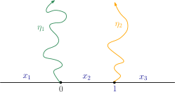
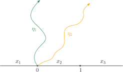
Figure 4: Left: Suppose $h$ is a Dirichlet GFF with piecewise constant boundary condition $x_{1}\textbf{1}_{(-\infty,0)}(x)+x_{2}\textbf{1}_{[0,1)}(x)+x_{3}\textbf{1}_{[1,+\infty)}(x)$. Let $\eta_{1}$ (resp. $\eta_{2}$) be the flow line of $h$ starting from 0 (resp. 1) of angle $\theta_{1}$ (resp. $\theta_{2}$). Then the marginal law of $\eta_{1}$ is SLE${}_{\kappa}(-\frac{x_{1}+\theta_{1}\chi}{\lambda}-1;\frac{x_{2}+\theta_{1}\chi}{\lambda}-1,\frac{x_{3}-x_{2}}{\lambda})$ with force points at $(0^{-};0^{+},1)$, and the marginal law of $\eta_{2}$ is SLE${}_{\kappa}(-\frac{x_{2}+\theta_{2}\chi}{\lambda}-1,\frac{x_{2}-x_{1}}{\lambda};\frac{x_{3}+\theta_{2}\chi}{\lambda}-1)$ force points at $(1^{-},0;1^{+})$. Suppose $\theta_{1}\geq\theta_{2}$. By [MS16a, Section 6], one can also read the conditional law of $\eta_{1}$ given $\eta_{2}$, which is SLE${}_{\kappa}(-\frac{x_{1}+\theta_{1}\chi}{\lambda}-1;\frac{x_{2}+\theta_{1}\chi}{\lambda}-1,\frac{-\theta_{2}\chi-x_{2}}{\lambda}-1)$ in the left component of $\mathbb{H}\backslash\eta_{2}$, and similarly conditional law of $\eta_{2}$ given $\eta_{1}$ is SLE${}_{\kappa}(-\frac{x_{2}+\theta_{2}\chi}{\lambda}-1,\frac{x_{2}+\theta_{1}\chi}{\lambda}-1;\frac{x_{3}+\theta_{2}\chi}{\lambda}-1)$ in the right component of $\mathbb{H}\backslash\eta_{1}$. If $\theta_{1}<\theta_{2}$, then given $\eta_{2}$, the segment of $\eta_{1}$ before crossing $\eta_{2}$ is the same as non-crossing case and $\eta_{1}$ can be continued after crossing. Finally, by the resampling property, the conditional laws of $\eta_{1}|\eta_{2}$ and $\eta_{2}|\eta_{1}$ uniquely characterize the joint distribution of $(\eta_{1},\eta_{2})$, as constructed using Imaginary Geometry. Right: One can similarly consider the flow lines from 0 and read off the marginal and conditional laws as in Lemma 3.3.

3.3 Reversibility of SLE${}_{\kappa}(\rho_{-};\rho_{+},\rho_{1})$

In this section, as an application of the Imaginary Geometry flow lines and the curve resampling properties, we extend the result on reversibility of SLE${}_{\kappa}(0;\rho_{+},\rho_{1})$ in [Zha22] to SLE${}_{\kappa}(\rho_{-};\rho_{+},\rho_{1})$ curves.

To begin with, let us recall the notion of SLE weighted by conformal derivative. Given $\rho_{-},\rho_{+}>-2$, $\rho_{1}>-2-\rho_{+}$ (which implies that the continuation threshold is never hit) and $\alpha\in\mathbb{R}$, we define the measure $\widetilde{\mathrm{SLE}}_{\kappa}(\rho_{-};\rho_{+},\rho_{1};\alpha)$ on curves $\eta$ from 0 to $\infty$ on $\mathbb{H}$ as follows. Let $D_{\eta}$ be the component of $\mathbb{H}\backslash\eta$ containing $1$, and $\psi_{\eta}$ the unique conformal map from $D_{\eta}$ to $\mathbb{H}$ fixing 1 and sending the first (resp. last) point on $\partial D_{\eta}$ hit by $\eta$ to 0 (resp. $\infty$). Then our $\widetilde{\mathrm{SLE}}_{\kappa}(\rho_{-};\rho_{+},\rho_{1};\alpha)$ on $\mathbb{H}$ is defined by

$$\frac{d\widetilde{\mathrm{SLE}}_{\kappa}(\rho_{-};\rho_{+},\rho_{1};\alpha)}{d{\mathrm{SLE}}_{\kappa}(\rho_{-};\rho_{+},\rho_{1})}(\eta)=|\psi_{\eta}(1)^{\prime}|^{\alpha}$$ (3.5)

where the force points of ${\mathrm{SLE}}_{\kappa}(\rho_{-};\rho_{+},\rho_{1})$ is $0^{-},0^{+},1$. This definition can be extended to other domains via conformal transforms, while by symmetry, we can also define the version $d\widetilde{\mathrm{SLE}}_{\kappa}(\rho_{-},\rho_{-1};\rho_{+};\alpha)$ with $1$ replaced by $-1$ and force points $-1,0^{-},0^{+}$ similarly. Also let $\mathcal{R}(\eta)$ be the time reversal of $\eta$. With these notations, we state the result in [Zha22] as follows.

Theorem 3.2.

Suppose $\eta$ an $\mathrm{SLE}_{\kappa}(0;\rho_{+},\rho_{1})$ curve in $\mathbb{H}$ from $0$ to $\infty$ with force located at $0^{+}$ and 1, and $\rho_{+}>-2,\rho_{+}+\rho_{1}>-2$. Let $\mathcal{L}$ be the law of the time reversal $\mathcal{R}(\eta)$ under the conformal mapping $z\mapsto-\frac{1}{z}$. Then $\mathcal{L}$ is a constant multiple of the measure $\widetilde{\mathrm{SLE}}_{\kappa}(\rho_{+}+\rho_{1},-\rho_{1};0;\frac{\rho_{1}(4-\kappa)}{2\kappa})$.

We note that the theorem above is implicitly shown in Theorem 1.1 and Section 3.2 of [Zha22] via the construction of the reversed curve. The statement is for general $\mathrm{SLE}_{\kappa}(\underline{\rho})$ curves with all force points lying on the same side of 0, while in this paper we only work on the $0^{+},1$ force point case for simplicity. To prove Theorem 1.5, we begin with the following variant of Proposition 3.1. Again suppose we want to sample $\eta_{2}\sim\widetilde{\mathrm{SLE}}_{\kappa}(\rho_{-};\rho_{+},\rho_{1};\alpha)$ to the right of $\eta_{1}$ in $\mathbb{H}\backslash\eta_{1}$ when $\eta_{1}$ is hitting $(0,\infty)$, let $p,q$ be the left and right most point on $\mathbb{R}$ on the boundary of the connected component of $D_{\eta_{1}}$. In each component of $\mathbb{H}\backslash\eta_{1}$ whose boundary contains a segment of $(0,p)$ (resp. $(q,\infty)$), we sample an independent $\mathrm{SLE}_{\kappa}(\rho_{-};\rho_{+})$ (resp. $\mathrm{SLE}_{\kappa}(\rho_{-};\rho_{+}+\rho_{1})$), and in $D_{\eta_{1}}$ we sample an $\widetilde{\mathrm{SLE}}_{\kappa}(\rho_{-};\rho_{+},\rho_{1};\alpha)$ curve from $p$ to $q$. Then $\eta_{2}$ is the concatenation of these curves.

Lemma 3.3.

Let $x_{1},x_{2},x_{3},\alpha,\theta_{1},\theta_{2}\in\mathbb{R}$ such that

$$\theta_{1}>\theta_{2};\ x_{1}<\lambda-\theta_{1}\chi;\ x_{2},x_{3}>-\lambda-\theta_{2}\chi.$$

The following two laws on pairs of curves $(\eta_{1},\eta_{2})$ agree:

• Sample $\eta_{1}$ in $\mathbb{H}$ from $0$ to $\infty$ as $\widetilde{\mathrm{SLE}}_{\kappa}(-\frac{x_{1}+\theta_{1}\chi}{\lambda}-1;\frac{x_{2}+\theta_{1}\chi}{\lambda}-1,\frac{x_{3}-x_{2}}{\lambda};\alpha)$. In $\mathbb{H}\backslash\eta_{1}$ in the region to the right of $\eta_{1}$, sample $\eta_{2}$ from $0$ to $\infty$ as $\widetilde{\mathrm{SLE}}_{\kappa}(-\frac{(\theta_{1}-\theta_{2})\chi}{\lambda}-2;\frac{x_{2}+\theta_{2}\chi}{\lambda}-1,\frac{x_{3}-x_{2}}{\lambda};\alpha)$.

• Sample $\eta_{2}$ in $\mathbb{H}$ from $0$ to $\infty$ as $\widetilde{\mathrm{SLE}}_{\kappa}(-\frac{x_{1}+\theta_{2}\chi}{\lambda}-1;\frac{x_{2}+\theta_{2}\chi}{\lambda}-1,\frac{x_{3}-x_{2}}{\lambda};\alpha)$. In $\mathbb{H}\backslash\eta_{2}$ in the region to the left of $\eta_{2}$, sample $\eta_{1}$ from $0$ to $\infty$ as $\mathrm{SLE}_{\kappa}(-\frac{x_{1}+\theta_{1}\chi}{\lambda}-1;\frac{(\theta_{1}-\theta_{2})\chi}{\lambda}-2)$.

Proof.

For $\alpha=0$ case, the result is straightforward from the flow line conditioning argument in [MS16a, Section 6] as drawn in Figure 4. If $\alpha\neq 0$, let $\mathcal{P}$ be the measure on curves $(\hat{\eta}_{1},\hat{\eta}_{2})$ as in the statement with $\alpha=0$. If we let $\mathcal{L}$ be the joint law of $(\eta_{1},\eta_{2})$ constructed from the second way (i.e. start with $\eta_{2}$ then sample $\eta_{1}$)

$$\frac{d\mathcal{L}}{d\mathcal{P}}(\eta_{1},\eta_{2})=|\psi_{\eta_{2}}^{\prime}(1)|^{\alpha}.$$ (3.6)

Meanwhile, if we first sample $\eta_{1}$ and then $\eta_{2}$ conditioned on $\eta_{1}$ as in the statement and let $\tilde{\mathcal{L}}$ be the joint law of $(\eta_{1},\eta_{2})$, then

$$\frac{d\tilde{\mathcal{L}}}{d\mathcal{P}}({\eta}_{1},{\eta}_{2})=|\psi_{{\eta}_{1}}^{\prime}(1)|^{\alpha}|\psi_{{\eta}_{2}|{\eta}_{1}}^{\prime}(1)|^{\alpha}$$ (3.7)

where $\psi_{{\eta}_{2}|{\eta}_{1}}$ is the conformal map from the component of $\mathbb{H}\backslash\psi_{{\eta}_{1}}({\eta}_{2})$ containing 1 to $\mathbb{H}$ fixing 1 and sending the first (resp. last) point hit by $\psi_{{\eta}_{1}}({\eta}_{2})$ to 0 (resp. $\infty$). Then we observe that $\psi_{{\eta}_{2}}=\psi_{{\eta}_{2}|{\eta}_{1}}\circ\psi_{{\eta}_{1}}$ and therefore the two Radon-Nikodym derivatives (3.6) and (3.7) are the same. ∎

Proof of Theorem 1.5.

We start with the case $\rho_{-}\leq 0$. We sample a curve $\eta_{1}$ from $\widetilde{\mathrm{SLE}}_{\kappa}(\rho_{+}+\rho_{1},-\rho_{1};0;\frac{\rho_{1}(4-\kappa)}{2\kappa})$ and a curve $\eta_{2}\sim\mathrm{SLE}_{\kappa}(\rho_{-};-\rho_{-}-2)$ with force points at $0^{-};0^{+}$ on the right component of $\mathbb{H}\backslash\eta_{1}$. Then by Theorem 3.2 we know that the marginal law of $\mathcal{R}(\eta_{1})$ is now $\mathrm{SLE}_{\kappa}(0;\rho^{+},\rho_{1})$; furthermore, by [MS16b, Theorem 1.1], the conditional law of $\mathcal{R}(\eta_{2})$ given $\mathcal{R}(\eta_{1})$ is $\mathrm{SLE}_{\kappa}(-\rho_{-}-2;\rho_{-})$. Therefore by Lemma 3.3, the conditional law of $\mathcal{R}(\eta_{1})$ given $\mathcal{R}(\eta_{2})$ is precisely $\mathrm{SLE}_{\kappa}(\rho_{-};\rho_{+},\rho_{1})$. See Figure 5.

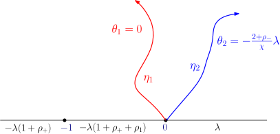
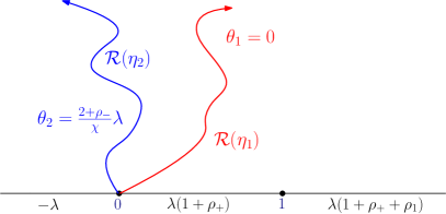
Figure 5: Left: The curves $(\eta_{1},\eta_{2})$, whose the law has Radon-Nikodym derivative $|\psi_{\eta_{1}}^{\prime}(-1)|^{\frac{\rho_{1}(4-\kappa)}{2\kappa}}$ with respect to the corresponding flow lines of the GFF with the depicted boundary values. By Lemma 3.3 the conditional law of $\eta_{1}$ given $\eta_{2}$ is $\widetilde{\mathrm{SLE}}_{\kappa}(\rho_{+}+\rho_{1},-\rho_{1};\rho_{-};\frac{\rho_{1}(4-\kappa)}{2\kappa})$. Right: An Imaginary Geometry coupling of $\mathcal{R}(\eta_{1})$ and $\mathcal{R}(\eta_{2})$ where the marginal law of $\mathcal{R}(\eta_{1})$ is $\mathrm{SLE}_{\kappa}(0;\rho^{+},\rho_{1})$ by Theorem 3.2 and the law of $\mathcal{R}(\eta_{2})$ given $\mathcal{R}(\eta_{1})$ is $\mathrm{SLE}_{\kappa}(-\rho_{-}-2;\rho_{-})$. Another application of Lemma 3.3 gives that the law of $\mathcal{R}(\eta_{1})$ given $\eta_{2}$ is $\mathrm{SLE}_{\kappa}(\rho_{-};\rho_{+},\rho_{1})$.

Now suppose $\rho^{-}\in[0,2]$. We first sample a curve $\eta_{2}$ on $\mathbb{H}$ from 0 to $\infty$ from $\widetilde{\mathrm{SLE}}_{\kappa}(2+\rho_{+}+\rho_{1},-\rho_{1};\rho_{-}-2;\frac{\rho_{1}(4-\kappa)}{2\kappa})$ and then $\eta_{1}$ from $\widetilde{\mathrm{SLE}}_{\kappa}(\rho_{+}+\rho_{1},-\rho_{1};0;\frac{\rho_{1}(4-\kappa)}{2\kappa})$ on the left component of $\mathbb{H}\backslash\eta_{2}$. Then using the same conformal map composing argument, we observe that the Radon-Nikodym derivative of the law of $(\eta_{1},\eta_{2})$ with respect to the flow lines of the GFF with the corresponding boundary values in Figure 6 is $|\psi_{\eta_{1}}^{\prime}(-1)|^{\frac{\rho_{1}(4-\kappa)}{2\kappa}}$, and the marginal law of $\eta_{1}$ is $\widetilde{\mathrm{SLE}}_{\kappa}(\rho_{+}+\rho_{1},-\rho_{1};\rho_{-};\frac{\rho_{1}(4-\kappa)}{2\kappa})$. By Theorem 3.2, we know that the conditional law of $\mathcal{R}(\eta_{1})$ given $\mathcal{R}(\eta_{2})$ is $\mathrm{SLE}_{\kappa}(0;\rho_{+},\rho_{1})$, while by what we have just proved, since $\rho_{-}-2\leq 0$, the marginal law of $\mathcal{R}(\eta_{2})$ is $\mathrm{SLE}_{\kappa}(\rho_{-}-2;2+\rho^{+},\rho_{1})$. Therefore using the Imaginary Geometry coupling we observe that the marginal law of $\mathcal{R}(\eta_{1})$ is $\mathrm{SLE}_{\kappa}(\rho_{-};\rho_{+},\rho_{1})$, which concludes the proof for $\rho_{-}\in[0,2]$ case. Also see Figure 6 for an illustration.

Finally we notice that the above argument (i.e., the coupling in Figure 6) can be iterated, giving the reversibility for $\rho_{-}\in[2,4],[4,6]$, …, etc.. This finishes the proof of Theorem 1.5.

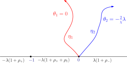
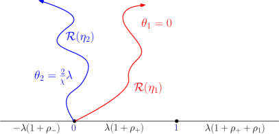
Figure 6: Left: The curves $(\eta_{1},\eta_{2})$, whose the law has Radon-Nikodym derivative $|\psi_{\eta_{1}}^{\prime}(-1)|^{\frac{\rho_{1}(4-\kappa)}{2\kappa}}$ with respect to the corresponding flow lines of the GFF with the depicted boundary values. One can show that the marginal law of $\eta_{1}$ is $\widetilde{\mathrm{SLE}}_{\kappa}(\rho_{+}+\rho_{1},-\rho_{1};\rho_{-};\frac{\rho_{1}(4-\kappa)}{2\kappa})$. Right: An Imaginary Geometry coupling of $\mathcal{R}(\eta_{1})$ and $\mathcal{R}(\eta_{2})$ where the marginal law of $\mathcal{R}(\eta_{2})$ is $\mathrm{SLE}_{\kappa}(\rho_{-}-2;2+\rho^{+},\rho_{1})$ and the conditional law of $\mathcal{R}(\eta_{1})$ given $\mathcal{R}(\eta_{2})$ is $\mathrm{SLE}_{\kappa}(0;\rho_{+},\rho_{1})$. Then we see that the marginal law of $\mathcal{R}(\eta_{1})$ is $\mathrm{SLE}_{\kappa}(\rho_{-};\rho_{+},\rho_{1})$.

∎

4 Conformal welding of $\mathrm{QT}(W,W,2)$ and two thin quantum disks

The aim of this section is to prove the following result. See Figure 7 for an illustration.

Theorem 4.1.

Fix $W>\frac{\gamma^{2}}{2}$ and $U\in(0,\frac{\gamma^{2}}{2})$. Take a triangle from $\mathrm{QT}(W+U,W+U,2+2U)$ embedded as $(\mathbb{H},\phi,0,\infty,1)$ with 1 being the weight $2+2U$ point. Then there exists some constant $c$ depending only on $W$ and $U$, and some probability measure $\mathsf{m}(W;U)$ of pairs of curves $(\eta_{1},\eta_{2})$ where $\eta_{1}$ runs from 1 to 0 and $\eta_{2}$ runs from 1 to $\infty$ such that the following welding equation holds:

$$\mathrm{QT}(W+U,W+U,2+2U)\otimes\mathsf{m}(W;U)=c\int_{0}^{\infty}\int_{0}^{\infty}\mathrm{Weld}(\mathrm{QT}(W,W,2;\ell,\ell^{\prime}),{\mathcal{M}}^{\mathrm{disk}}_{2}(U;\ell),{\mathcal{M}}^{\mathrm{disk}}_{2}(U;\ell^{\prime})d\ell d\ell^{\prime}$$ (4.1)

where $\mathrm{QT}(W,W,2;\ell,\ell^{\prime})$ is disintegration over the length of the two boundary arcs containing the weight 2 vertex and $\mathrm{Weld}$ stands for identifying the edges of lengths $\ell$, $\ell^{\prime}$.

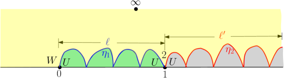
Figure 7: Setup of Theorem 4.1. We claim that welding a thick disk from ${\mathcal{M}}^{\mathrm{disk}}_{2,\bullet}(W)$ (which is the same as $\mathrm{QT}(W,W,2)$) with two weight $U$ thin disks along the boundary arc containing the third marked point produces a three-pointed disk with law $\mathrm{QT}(W+U,W+U,2+2U)$ embedded as $(\mathbb{H},\phi,0,\infty,1)$.

This section is organized as follows. In Section 4.1 we recall the notion of conformal welding and the result from [AHS21, Proposition 4.5], which states the welding of a two-pointed disk with a three-pointed disk. Then using a limiting procedure over this result, in Section 4.2 we give the proof of Theorem 4.1.

4.1 Conformal welding of two-pointed and three-pointed disks

We first recall the the conformal welding of quantum surfaces. Let $n\geq 1$ and $\mathcal{M}^{1},...,\mathcal{M}^{n}$ be measures on quantum surfaces. Fix some boundary arcs $\tilde{e}_{1},e_{1},...,\tilde{e}_{n},e_{n}$ such that $e_{i}$ and $\tilde{e}_{i}$ are different boundary arcs on samples from $\mathcal{M}_{i}$. Suppose we have the disintegration

$$\mathcal{M}^{i}=\int_{0}^{\infty}\int_{0}^{\infty}\mathcal{M}^{i}(\ell_{i-1},\ell_{i})d\ell_{i}d\ell_{i-1}\ \ \text{for}\ \ i=1,...,n$$

over the quantum lengths of $e_{i}$ and $\tilde{e}_{i}$. Given a tuple of independent surfaces from $\mathcal{M}^{1}(\ell_{0},\ell_{1})\times\mathcal{M}^{2}(\ell_{1};\ell_{2})\times\cdots\mathcal{M}^{n}(\ell_{n-1},\ell_{n})$, suppose that they can a.s. be conformally welded along the pairs of arcs $(e_{1},\tilde{e}_{i+1})$ for $i=1,...,n-1$, yielding a large surface decorated with interfaces from the gluing. We write

$$\text{Weld}(\mathcal{M}^{1}(\ell_{0},\ell_{1}),\mathcal{M}^{2}(\ell_{1},\ell_{2}),...,\mathcal{M}^{n}(\ell_{n-1},\ell_{n}))$$

for the law of the resulting curve-decorated surface. On the other hand, suppose we have a quantum surface sampled from some measure $\mathcal{M}$ and embedded on domain $D$ and we also sample an independent family of curves on $D$ from some measure $\mathcal{P}$ with conformal invariance property. Then we write $\mathcal{M}\otimes\mathcal{P}$ for the law of this curve-decorated surface.

We emphasize that for all the quantum surfaces discussed in this paper, including the (two and three pointed) quantum disks and quantum triangles, the conformal welding as above is well-defined. This is because near a point $x$ with weight $W\geq\frac{\gamma^{2}}{2}$, the field is locally absolutely continuous to that of a weight $W$ quantum wedge near its finite-volume endpoint, while near a point $x$ with weight $W<\frac{\gamma^{2}}{2}$ the surface is a Possionian chain of weight $\gamma^{2}-W$ disks so local absolute continuity with respect to the weight $W$ quantum wedge still holds. Therefore from the conformal welding of quantum wedges [DMS21, Theorem 1.2], our conformal weldings for quantum disks and triangles are well-defined. See e.g. [She16], [DMS21, Section 3.5] or [GHS19, Section 4.1] for more background on conformal welding.

We state the conformal welding of two-pointed quantum disks as below. Recall the notion of the measure $\mathcal{P}^{\text{disk}}(W_{1},...,W_{n})$ in [AHS20, Definition 2.25] on tuple of curves $(\eta_{1},...,\eta_{n-1})$ in a domain $(D,x,y)$, which is the same as $\textup{SLE}_{\kappa}(W_{1}-2;W_{2}-2)$ from $x$ to $y$ for $n=2$ and defined recursively for $n\geq 3$ by first sampling $\eta_{n-1}$ from $\textup{SLE}_{\kappa}(W_{1}+...+W_{n-1}-2;W_{n}-2)$ then $(\eta_{1},...,\eta_{n-2})$ from $\mathcal{P}^{\text{disk}}(W_{1},...,W_{n-1})$ on each connected component $(D^{\prime},x^{\prime},y^{\prime})$ on the left of $D\backslash\eta_{n-1}$ where $x^{\prime}$ and $y^{\prime}$ are the first and the last point hit by $\eta_{n-1}$.

Theorem 4.2 (Theorem 2.2 of [AHS20]).

Fix $W_{1},...,W_{n}>0$ and $W=W_{1}+...+W_{n}$. Then there exists a constant $c=c_{W_{1},...,W_{n}}\in(0,\infty)$ such that for all $\ell,r>0$, the identity

$$\begin{split}&\mathcal{M}_{2}^{\textup{disk}}(W;\ell,r)\otimes\mathcal{P}^{\textup{disk}}(W_{1},...,W_{n})\\ &=c\iiint_{0}^{\infty}\textup{Weld}(\mathcal{M}_{2}^{\textup{disk}}(W_{1};\ell,\ell_{1}),\mathcal{M}_{2}^{\textup{disk}}(W_{2};\ell_{1},\ell_{2}),...,\mathcal{M}_{2}^{\textup{disk}}(W_{n};\ell_{n-1},r))d\ell_{1}...d\ell_{n-1}\end{split}$$ (4.2)

holds as measures on the space of curve-decorated quantum surfaces.

Next we present the welding of two-pointed quantum disk with three-pointed quantum disks as in [AHS21, Proposition 4.5], which adds a marked point to the boundary arc in Theorem 4.2 above. Recall the notion of SLE weighted by conformal radius in Section 3.3.

Proposition 4.3.

Suppose $W_{1},W_{2}>0$, $W_{1}+W_{2}\neq\frac{\gamma^{2}}{2}$ and $W_{2}\neq\frac{\gamma^{2}}{2}$. Then there exists a constant $c_{W_{1},W_{2}}\in(0,\infty)$ such that for all $\beta\in\mathbb{R}$ and $\ell>0$,

$$\begin{split}\mathcal{M}_{2,\bullet}^{\textup{disk}}(W_{1}+W_{2};\beta;\ell)&\otimes\widetilde{\mathrm{SLE}}_{\kappa}(W_{1}-2;W_{2}-2,0;1-\Delta_{\beta})\\ &=c_{W_{1},W_{2}}\int_{0}^{\infty}\textup{Weld}(\mathcal{M}_{2}^{\textup{disk}}(W_{1};\ell,x),\mathcal{M}_{2,\bullet}^{\textup{disk}}(W_{2};\beta;x))dx.\end{split}$$ (4.3)

where again $\Delta_{\beta}$ is determined by (2.8).

Note that if $W_{1}+W_{2}<\frac{\gamma^{2}}{2}$, the interface above is understood as a chain of $\mathrm{SLE}_{\kappa}(W_{1}-2;W_{2}-2)$ curves except that the segment of curve on the disk containing the marked point is replaced by $\widetilde{\mathrm{SLE}}_{\kappa}(W_{1}-2;W_{2}-2,0;1-\Delta_{\beta})$. If $\alpha=\gamma$ then since $\Delta_{\gamma}=1$, the interface is simply $\mathrm{SLE}_{\kappa}(W_{1}-2;W_{2}-2)$ without any reweighting.

Proof.

When $W_{1}\geq\frac{\gamma^{2}}{2}$, the statement is precisely the same as [AHS21, Proposition 4.5]. Now suppose $W_{1}<\frac{\gamma^{2}}{2}$. We start with a sample from $\mathcal{M}_{2,\bullet}^{\textup{disk}}(2+W_{1}+W_{2};\beta)$ embedded as $(\mathbb{H},\phi,0,\infty,1)$ where the $\beta$-insertion is located at 1. Sample an independent curve $\eta_{2}$ from $\widetilde{\mathrm{SLE}}_{\kappa}(W_{1},W_{2}-2;1-\Delta_{\beta})$, and given $\eta_{2}$, independently sample a curve $\eta_{1}$ from SLE${}_{\kappa}(0;W_{1}-2)$ on the left component of $\mathbb{H}\backslash\eta_{2}$. Let $\tilde{\mathcal{P}}(2,W_{1},W_{2})$ be the joint law of $(\eta_{1},\eta_{2})$. Then by Theorem 4.2, we obtain that for some $c=c_{W_{1},W_{2}}\in(0,\infty)$,

$$\mathcal{M}_{2,\bullet}^{\textup{disk}}(2+W_{1}+W_{2};\beta)\otimes\tilde{\mathcal{P}}(2,W_{1},W_{2})=c\iint_{[0,\infty)^{2}}\text{Weld}(\mathcal{M}_{2}^{\textup{disk}}(2;\ell),\mathcal{M}_{2}^{\textup{disk}}(W_{1};\ell,x),\mathcal{M}_{2,\bullet}^{\textup{disk}}(W_{2};\beta;x))dxd\ell.$$ (4.4)

On the other hand, using the same trick as in the proof of Theorem 1.5, the marginal law of $\eta_{1}$ under $\tilde{\mathcal{P}}$ is $\widetilde{\mathrm{SLE}}_{\kappa}(0;W_{1}+W_{2}-2,0;1-\Delta_{\beta})$, and by the existing argument for $W_{1}\geq\frac{\gamma^{2}}{2}$, given the interface and its quantum length $\ell$, the quantum surface to the right of $\eta_{1}$ has law $\mathcal{M}_{2,\bullet}^{\textup{disk}}(W_{1}+W_{2};\beta;\ell)$. The law of $\eta_{2}$ given $\eta_{1}$ is $\widetilde{\mathrm{SLE}}_{\kappa}(W_{1}-2;W_{2}-2,0;1-\Delta_{\beta})$ on the right component of $\mathbb{H}\backslash\eta_{1}$, and therefore disintegrating (4.4) over $\ell$ and $\eta_{1}$ yields the proposition. ∎

Recall from Remark 2.19, if $W_{3}>\frac{\gamma^{2}}{2}$ and $\beta_{3}=\gamma+\frac{2-W_{3}}{\gamma}$, then the measure $\mathcal{M}_{2,\bullet}^{\textup{disk}}(W;\beta_{3};\ell)$ is some multiple constant of our quantum triangle QT$(W,W,W_{3};\ell)$. Therefore we can rewrite (4.3) as

$$\begin{split}\text{QT}(W_{1}+W_{2},W_{1}+W_{2},W_{3};\ell)&\otimes\widetilde{\mathrm{SLE}}_{\kappa}(W_{1}-2;W_{2}-2,0;1-\Delta_{\beta_{3}})=\\ &c_{W_{1},W_{2}}\int_{0}^{\infty}\textup{Weld}(\mathcal{M}_{2}^{\textup{disk}}(W_{1};\ell,x),\text{QT}(W_{2},W_{2},W_{3};x))dx.\end{split}$$ (4.5)

We emphasize that (4.5) continues to hold for $W_{3}<\frac{\gamma^{2}}{2}$ by the thick-thin duality. This is because concatenating weight $W_{3}$ quantum disks to both sides of (4.5) (with $W_{3}$ replaced by $\gamma^{2}-W_{3}$) does not affect the equation, while from (2.8), the corresponding $\Delta_{\beta}$’s are the same for $W_{3}$ and $\gamma^{2}-W_{3}$ and therefore the interfaces are the same.

4.2 Proof of Theorem 4.1

The idea of proving Theorem 4.1 is as follows. First assume $W\in(\frac{\gamma^{2}}{2},2)$ and $U\in(0,\frac{\gamma^{2}}{2})$. We take $(W_{1},W_{2})$ to be $(W,U)$ in Proposition 4.3 and let $\beta\downarrow\beta_{0}:=\gamma-\frac{2U}{\gamma}$. In this limiting procedure, we will show that the SLE excursion containing the point 1 shrinks into a single point, yielding the desired welding picture. Finally if $W>2$, we can split the weight $W$ disk into a weight $W-2$ quantum disk and a weight $2$ quantum disk and apply Proposition 4.3.

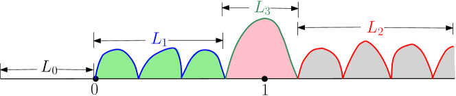
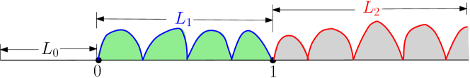
Figure 8: Illustration of the proof of Theorem 4.1. Top: A three-pointed disk from ${\mathcal{M}}^{\mathrm{disk}}_{2,\bullet}(W+U;\beta;\ell_{0})$ embedded as $(\mathbb{H},\phi,0,\infty,1)$ decorated by an independent $\widetilde{\mathrm{SLE}}_{\kappa}(W-2;U-2,0;1-\Delta_{\beta})$ curve on the top. This splits the surface into a weight $W$ thick disk and a three-pointed disk of weight $U$, which can further be decomposed into two weight $U$ disks (on the left and right of 1) and a disk from ${\mathcal{M}}^{\mathrm{disk}}_{2,\bullet}(\gamma^{2}-U;\beta)$. Bottom: As $\beta\downarrow\beta_{0}$, the disk containing the point 1 shrinks to a single point, yielding the picture in Theorem 4.1.

Consider a three-pointed quantum disk from ${\mathcal{M}}^{\mathrm{disk}}_{2,\bullet}(W+U;\beta;\ell_{0})^{\#}$ embedded as $(\mathbb{H},\phi_{\beta},0,\infty,1)$ (with 1 being the $\beta$-insertion and $\ell_{0}$ being the quantum length of $(-\infty,0)$), and draw an independent curve $\eta$ from $\widetilde{\mathrm{SLE}}_{\kappa}(W-2;U-2,0;1-\Delta_{\beta})^{\#}$. Note that by [AHS21, Theorem 1.1] $|\widetilde{\mathrm{SLE}}_{\kappa}(W-2;U-2,0;1-\Delta_{\beta})|<\infty$ for $\beta\in(\beta_{0},\gamma)$ and $|\widetilde{\mathrm{SLE}}_{\kappa}(W-2;U-2,0;1-\Delta_{\beta_{0}})|=\infty$. This curve is boundary-hitting, and let $\tau$ (resp. $\sigma$) be the start (resp. end) time of the excursion containing the point 1. Let $L_{1}$, $L_{2}$, $L_{3}$ be the quantum lengths of $\eta|_{[0,\tau]}$,$\eta|_{[\sigma,\infty)}$ and $\eta|_{[\tau,\sigma]}$. (See also Figure 8.) By Proposition 4.3, given the interface $\eta$ and its quantum length $\ell$, the surface above $\eta$ is a weight $W$ quantum disk from ${\mathcal{M}}^{\mathrm{disk}}_{2}(W;\ell)$, while the beaded surface below $\eta$ is a three-pointed quantum disk from ${\mathcal{M}}^{\mathrm{disk}}_{2,\bullet}(U;\beta;\ell)$, which by Definition 2.16 can further be realized as ${\mathcal{M}}^{\mathrm{disk}}_{2}(U)\times{\mathcal{M}}^{\mathrm{disk}}_{2}(\gamma^{2}-U;\beta)\times{\mathcal{M}}^{\mathrm{disk}}_{2}(U)$.

Lemma 4.4.

In the above setting, assume $W\in(\frac{\gamma^{2}}{2},2)$ and $\beta<\gamma$. Then as $\beta\downarrow\beta_{0}$, under the normalized measure ${\mathcal{M}}^{\mathrm{disk}}_{2,\bullet}(W+U;\beta;\ell_{0})^{\#}\otimes\widetilde{\mathrm{SLE}}_{\kappa}(W-2;U-2,0;1-\Delta_{\beta})^{\#}$, $\ell_{3}$ converges to 0 in probability.

Proof.

From Proposition 2.24 we know that $|{\mathcal{M}}^{\mathrm{disk}}_{2,\bullet}(W+U;\beta;\ell_{0})|$ is finite for $\beta\in[\beta_{0},\gamma]$ while $|\widetilde{\mathrm{SLE}}_{\kappa}(W-2;U-2,0;1-\Delta_{\beta_{0}})|=\infty$, it suffices to prove that for any $\varepsilon>0$, there is some constant $C>0$ not depending on $\beta\in(\beta_{0},\gamma)$ such that under ${\mathcal{M}}^{\mathrm{disk}}_{2,\bullet}(W+U;\beta;\ell_{0})\otimes\widetilde{\mathrm{SLE}}_{\kappa}(W-2;U-2,0;1-\Delta_{\beta})$, the event $\{\ell_{3}>\varepsilon\}$ has measure no larger than $C$.

By Proposition 4.3 and Definition 2.16, there exists some constants $c$ depending only on $\gamma,U,W$ (which might vary in the lines of the equation) but not on $\beta$ such that

$$\begin{split}&\ \ \ \ \big{(}{\mathcal{M}}^{\mathrm{disk}}_{2,\bullet}(W+U;\beta;\ell_{0})\otimes\widetilde{\mathrm{SLE}}_{\kappa}(W-2;U-2,0;1-\Delta_{\beta})\big{)}\big{[}\ell_{3}>\varepsilon\big{]}\\ &=c\int_{\varepsilon}^{\infty}\int_{0}^{\infty}\int_{0}^{\infty}|{\mathcal{M}}^{\mathrm{disk}}_{2}(W;\ell_{0},\ell_{1}+\ell_{2}+\ell_{3})||{\mathcal{M}}^{\mathrm{disk}}_{2}(U;\ell_{1})||{\mathcal{M}}^{\mathrm{disk}}_{2}(U;\ell_{2})||{\mathcal{M}}^{\mathrm{disk}}_{2}(\gamma^{2}-U;\beta;\ell_{3})|d\ell_{1}d\ell_{2}d\ell_{3}\\ &=c\int_{\varepsilon}^{\infty}\int_{\varepsilon}^{\ell}\int_{0}^{\ell-\ell_{3}}|{\mathcal{M}}^{\mathrm{disk}}_{2}(W;\ell_{0},\ell)|\ell_{1}^{-\frac{2U}{\gamma^{2}}}(\ell-\ell_{3}-\ell_{1})^{-\frac{2U}{\gamma^{2}}}\ell_{3}^{\frac{1}{\gamma}(\beta-\gamma+\frac{2U}{\gamma})-1}d\ell_{1}d\ell_{3}d\ell\\ &=c\int_{\varepsilon}^{\infty}\int_{\varepsilon}^{\ell}|{\mathcal{M}}^{\mathrm{disk}}_{2}(W;\ell_{0},\ell)|(\ell-\ell_{3})^{-\frac{4U}{\gamma^{2}}+1}\ell_{3}^{\frac{1}{\gamma}(\beta-\gamma+\frac{2U}{\gamma})-1}d\ell_{3}d\ell\\ &=c\int_{\varepsilon}^{\infty}|{\mathcal{M}}^{\mathrm{disk}}_{2}(W;\ell_{0},\ell)|\ell^{\frac{\beta}{\gamma}-\frac{2U}{\gamma^{2}}}\int_{\frac{\varepsilon}{\ell}}^{1}(1-x)^{-\frac{4U}{\gamma^{2}}+1}x^{\frac{1}{\gamma}(\beta-\beta_{0})-1}dxd\ell\end{split}$$ (4.6)

where in the third line we used Proposition 2.22 and Proposition 2.23. Now we fix $\delta>0$ small and observe that

$$\begin{split}&\int_{s}^{1}(1-x)^{-\frac{4U}{\gamma^{2}}+1}x^{\frac{1}{\gamma}(\beta-\beta_{0})-1}dx\leq s^{-\delta}\int_{0}^{1}(1-x)^{-\frac{4U}{\gamma^{2}}+1}x^{\frac{1}{\gamma}(\beta-\beta_{0})-1+\delta}dx\leq C(\delta)s^{-\delta}.\end{split}$$ (4.7)

Plugging (4.7) in, we observe that the quantity in (4.7) is controlled by

$$C\int_{\varepsilon_{0}}^{\infty}|{\mathcal{M}}^{\mathrm{disk}}_{2}(W;\ell_{0},\ell)|\ell^{\frac{\beta}{\gamma}-\frac{2U}{\gamma^{2}}+\delta}d\ell$$ (4.8)

where $C=C(\delta,\varepsilon,\gamma,W,U)$ is some constant. Now we take $\delta=\frac{U}{\gamma^{2}}$ so $\frac{\beta}{\gamma}-\frac{2U}{\gamma^{2}}+\delta$ varies between $(0,1-\frac{U}{\gamma^{2}})$. To conclude the proof, it suffices to verify that

$$\int_{0}^{\infty}|{\mathcal{M}}^{\mathrm{disk}}_{2}(W;\ell_{0},\ell)|\ell^{1-\frac{U}{\gamma^{2}}}d\ell<\infty.$$ (4.9)

We observe that by Proposition 2.24, a three-pointed disk from ${\mathcal{M}}^{\mathrm{disk}}_{2,\bullet}(\frac{U}{2};\gamma)$ (or equivalently $\mathrm{QT}(\frac{U}{2},\frac{U}{2},2)$) has unmarked boundary length law $c\ell^{1-\frac{U}{\gamma^{2}}}d\ell$, and by Proposition 4.3, (4.9) is a constant times

$$\int_{0}^{\infty}|{\mathcal{M}}^{\mathrm{disk}}_{2}(W;\ell_{0},\ell)||{\mathcal{M}}^{\mathrm{disk}}_{2,\bullet}(\frac{U}{2};\gamma;\ell)|d\ell=c|{\mathcal{M}}^{\mathrm{disk}}_{2,\bullet}(W+\frac{U}{2};\gamma;\ell_{0})|.$$ (4.10)

However, we know from Proposition 2.23 that $|{\mathcal{M}}^{\mathrm{disk}}_{2,\bullet}(W+\frac{U}{2};\gamma;\ell_{0})|<\infty$, which concludes the proof. ∎

The next lemma gives the interpretation of the right hand side of (4.1). We write $\bar{\mathcal{M}}_{2}(U)$ for the law of the surface constructed by concatenating a pair of samples from ${\mathcal{M}}^{\mathrm{disk}}_{2}(U)\times{\mathcal{M}}^{\mathrm{disk}}_{2}(U)$, giving the disintegration

$$\bar{\mathcal{M}}_{2}(U;\ell)=\int_{0}^{\ell}{\mathcal{M}}^{\mathrm{disk}}_{2}(U;r)\times{\mathcal{M}}^{\mathrm{disk}}_{2}(U;\ell-r)dr.$$ (4.11)

Lemma 4.5.

The triply marked surface on the right hand side of (4.1) is the same as

$$\int_{0}^{\infty}\mathrm{Weld}({\mathcal{M}}^{\mathrm{disk}}_{2}(W;\ell),\bar{\mathcal{M}}_{2}(U;\ell))d\ell.$$ (4.12)

Proof.

We start with a sample from ${\mathcal{M}}^{\mathrm{disk}}_{2}(W;\ell)$ where $\ell$ is its right boundary length. Then sample $r\sim\text{Leb}_{[0,\ell]}$ and mark the point on the right boundary arc with distance $r$ to the top endpoint. Recall that from Definition 2.13 and Proposition 2.14, once given $r$, after adding a third point onto the right boundary of weight $W$ disk, the law of the surface we get is precisely ${\mathcal{M}}^{\mathrm{disk}}_{2,\bullet}(W;r,\ell-r)$. Therefore the lemma follows by simultaneously welding a pair of samples from ${\mathcal{M}}^{\mathrm{disk}}_{2}(U;r)\times{\mathcal{M}}^{\mathrm{disk}}_{2}(U;\ell-r)$ to the right boundary arc according to quantum length and recalling the definition (4.11). ∎

We notice that as in the proof of Lemma 4.4,

$$|\int_{0}^{\infty}\mathrm{Weld}({\mathcal{M}}^{\mathrm{disk}}_{2}(W;\ell_{0},\ell),\bar{\mathcal{M}}_{2}(U;\ell))d\ell|=c\int_{0}^{\infty}|{\mathcal{M}}^{\mathrm{disk}}_{2}(W;\ell_{0},\ell)|\ell^{1-\frac{4U}{\gamma^{2}}}d\ell=c|{\mathcal{M}}^{\mathrm{disk}}_{2,\bullet}(W+2U;\ell_{0})|<\infty,$$ (4.13)

which means that we may sample a quantum surface from the normalized version of the measure on the right hand side of (4.1) embedded as $(\mathbb{H},\tilde{\phi},0,\infty,1)$ with $(\tilde{\eta}_{1},\tilde{\eta}_{2})$ being curves joining 1 with 0 and $\infty$. To prove the theorem, we need to show that the law of $(\mathbb{H},\tilde{\phi},0,\infty,1)$ is ${\mathcal{M}}^{\mathrm{disk}}_{2,\bullet}(W+U;\beta_{0};\ell_{0})^{\#}$, and $(\tilde{\eta}_{1},\tilde{\eta}_{2})$ are independent of the surface.

We go back to the setting as in Lemma 4.4 and Figure 8. Let $S_{\beta}$ be the connected component of $\mathbb{H}\backslash\eta$ containing 1, and $x_{\beta}$ be the quantum midpoint of the left boundary of $(\mathbb{H},\phi_{\beta},0,\infty,1)$ (i.e. $\nu_{\phi_{\beta}}((-\infty,x_{\beta}))=\nu_{\phi_{\beta}}((x_{\beta},0))=\frac{\ell_{0}}{2}$). Consider the conformal map $g_{\beta}$ from $\mathbb{H}\backslash S_{\beta}$ to $\mathbb{H}$ that fixes 0, $\infty$ and $x_{\beta}$. For any $\varepsilon>0$ let $\mathbb{H}_{\varepsilon}=\{z\in\mathbb{H}:|z-1|>\varepsilon\}$. Since it is clear that the law of $(\mathbb{H}_{\varepsilon},{\phi}_{\beta},0,\infty)$ converges in total variation to $(\mathbb{H}_{\varepsilon},{\phi}_{\beta_{0}},0,\infty)$ (which could be seen from the LCFT definition and the disintegration description in (2.33)), we may couple $(\mathbb{H}_{\varepsilon},{\phi}_{\beta},0,\infty)$ with $(\mathbb{H}_{\varepsilon},{\phi}_{\beta_{0}},0,\infty)$ such that the corresponding $x_{\beta}$ agrees with $x_{\beta_{0}}$ with probability $1-o_{\beta}(1)$. We shall work on the surface $(\mathbb{H}\backslash S_{\beta},0,\infty)$, which is equivalent to $(\mathbb{H},\hat{\phi}_{\beta},0,\infty)$ where $\hat{\phi}_{\beta}=\phi_{\beta}\circ g_{\beta}^{-1}+Q\log|(g_{\beta}^{-1})^{\prime}|$.

Lemma 4.6.

Fix $\varepsilon>0$. Under the measure ${\mathcal{M}}^{\mathrm{disk}}_{2,\bullet}(W+U;\beta;\ell_{0})^{\#}\otimes\widetilde{\mathrm{SLE}}_{\kappa}(W-2;U-2,0;1-\Delta_{\beta})^{\#}$, as $\beta\downarrow\beta_{0}$, the law of the surface $(\mathbb{H}_{\varepsilon},\hat{\phi}_{\beta},0,\infty)$ converges weakly to that of $(\mathbb{H}_{\varepsilon},\tilde{\phi},0,\infty)$.

Proof.

From Lemma 4.4, the quantum length of $\ell_{3}$ is converging in probability to zero, and therefore the claim follows directly from the continuity of the disintegration of quantum disks over quantum length (see e.g. [AHS20, Proposition 2.23] and [ARS21, Lemma 5.17]) and the description provided by Lemma 4.5. ∎

Proof of Theorem 4.1.

Step 1. Identifying the field. Assume that we are in the setting of Lemma 4.4 and 4.6, and $W\in(\frac{\gamma^{2}}{2},2]$. We prove that, for any $\varepsilon>0$, the distributions $\hat{\phi}_{\beta}$ converges weakly to $\phi_{\beta_{0}}$ in the domain $\mathbb{H}_{\varepsilon}$, where again $\phi_{\beta_{0}}$ is sampled from ${\mathcal{M}}^{\mathrm{disk}}_{2,\bullet}(W+U;\beta_{0};\ell_{0})^{\#}$. Then Lemma 4.6 implies that the law of $(\mathbb{H},\tilde{\phi},0,\infty,1)$ is $\mathrm{QT}(W+U,W+U,2+2U;\ell_{0})^{\#}$.

We start by extending $g_{\beta}$ to the conformal map from $\mathbb{C}\backslash(S_{\beta}^{*}\cup\mathbb{R}_{+})$ to $\mathbb{C}\backslash\mathbb{R}_{+}$ via Schwartz reflection, where $S_{\beta}^{*}=S_{\beta}\cup\{z:\bar{z}\in S_{\beta}\}$. Fix $\delta>0$ and work on the event that $x_{\beta}<-\delta$, which has probability $1-o_{\delta}(1)$. Then since the quantum length $\ell_{3}$ goes to 0 in probability, if we let $\beta\downarrow\beta_{0}$, the probability that an independent Brownian motion starting from $x-\beta$ exits $\mathbb{C}\backslash(S_{\beta}^{*}\cup\mathbb{R}_{+})$ through $\partial S_{\beta}$ goes to 0.

Consider the conformal map $\psi_{\beta}$ from $\mathbb{C}\backslash\mathbb{R}_{+}$ to the unit disk sending $x_{\beta}$ to 0 and $\infty$ to 1. Then the Beurling estimate (see e.g. [Law08, Section 3.8]) implies that for any fixed $\varepsilon>0$, with probability 1-$o_{\beta}(1)$, the set $\psi_{\beta}(S_{\beta}^{*})$ is contained in $\{z:1-\varepsilon<|z|<1\}$. This implies that the kernel of the set $\mathbb{C}\backslash(S_{\beta}^{*}\cup\mathbb{R}_{+})$ is $\mathbb{C}\backslash\mathbb{R}_{+}$ with probability $1-o_{\delta}(1)$, and the Carathéodory kernel theorem (see e.g. [Law08, Section 3.6]) implies that the conformal maps $g_{\beta}^{-1}$ converges uniformly on compact sets of $\mathbb{C}\backslash\mathbb{R}_{+}$ to the identity function. Then in $\mathbb{H}_{\varepsilon}$, since $\hat{\phi}_{\beta}=\phi_{\beta}\circ g_{\beta}^{-1}+Q\log|(g_{\beta}^{-1})^{\prime}|$ and $\phi_{\beta}$ converges in total variation distance to $\phi_{\beta_{0}}$, it is clear that as we first send $\beta\downarrow\beta_{0}$ and then $\delta\to 0$, $\hat{\phi}_{\beta}$ converges weakly to $\phi_{\beta_{0}}$, which concludes the first step of the proof.

Step 2. Identifying the interface. In Step 1 we have shown that in the $(\mathbb{H},\tilde{\phi},0,\infty,1)$ obtained by welding two weight $U$ disks with a weight $W$ disk, the field $\tilde{\phi}$ is precisely the Liouville field. Now we show that the law of the interfaces $(\tilde{\eta}_{1},\tilde{\eta}_{2})$ on the right hand side of (4.1) can be characterized by some SLE resampling property and independent of the field.

Recall that in curve-decorated surface ${\mathcal{M}}^{\mathrm{disk}}_{2,\bullet}(W+U;\beta;\ell_{0})\otimes\widetilde{\mathrm{SLE}}_{\kappa}(W-2;U-2,0;1-\Delta_{\beta})$, as we remove the bubble $S_{\beta}$, the interfaces $(\eta_{1},\eta_{2})$ are given by $(\eta|_{[0,\tau]},\eta|_{[\sigma,\infty)})$ where $\tau$ (resp. $\sigma$) be the start (resp. end) time of the excursion containing the point 1. Then by SLE Markov property, given $S_{\beta}$ and $\beta_{1}$, the law of $\eta_{2}$ is $\mathrm{SLE}_{\kappa}(W-2;U-2)$ with force points at $0$ and $\eta(\sigma)_{+}$ in the right connected component of $\mathbb{H}\backslash\eta|_{[0,\sigma]}$. Similarly, using the SLE reversibility statement [MS16b, Theorem 1.1], the law of $\eta_{1}$ given $S_{\beta}$ and $\eta_{2}$ is the $\mathrm{SLE}_{\kappa}(U-2;W-2)$ process from 1 to 0 in the left connected component of $\mathbb{H}\backslash\eta|_{[\tau,\infty)}$ with force points at $\eta(\tau)_{-}$ and $\infty$. Therefore it follows from Lemma 4.6 that the law of $\tilde{\eta}_{1}$ given $\tilde{\eta}_{2}$ is the $\mathrm{SLE}_{\kappa}(U-2;W-2)$ process from 1 to 0 in the left connected component of $\mathbb{H}\backslash\tilde{\eta}_{2}$ with force points at $1^{-}$ and $\infty$, while the law of $\tilde{\eta}_{2}$ given $\tilde{\eta}_{1}$ is the $\mathrm{SLE}_{\kappa}(W-2;U-2)$ process from 1 to $\infty$ in the left connected component of $\mathbb{H}\backslash\tilde{\eta}_{2}$ with force points at $0$ and $1^{+}$. Therefore it follows from the SLE resampling property (Proposition 3.1) that the joint law of $(\tilde{\eta}_{1},\tilde{\eta}_{2})$ is unique and independent of the field, and thus concluding the proof for $W\in(\frac{\gamma^{2}}{2},2]$.

Step 3. Extension to $W>2$. In Figure 7, by Theorem 4.2, we can weld the weight $W$ disk into a weight $W-2$ disk on the left and a weight 2 disk on the right with interface $\eta_{0}$. Then by Steps 1 and 2, the law of the quantum surface on the right of $\eta_{0}$ is a three-pointed disk ${\mathcal{M}}^{\mathrm{disk}}_{2,\bullet}(2+U;\beta_{0})$, and therefore by Proposition 4.3 the whole surface has law ${\mathcal{M}}^{\mathrm{disk}}_{2,\bullet}(W+U;\beta_{0})$. Moreover the marginal law of $\eta_{0}$ is $\widetilde{\mathrm{SLE}}_{\kappa}(W-4;U,0;1-\Delta_{\beta_{0}})$, while the law of the interfaces $(\eta_{1},\eta_{2})$ given $\eta_{0}$ are characterized by the SLE resampling properties. Therefore the law of $(\eta_{1},\eta_{2})$ is independent of the field, which concludes the proof of the Theorem. ∎

5 Proof of Theorem 1.2 for a restricted range

Theorem 5.1.

Suppose $0<U<\frac{\gamma^{2}}{2}<W$. Sample a curve-decorated quantum surface from

$$\int_{0}^{\infty}\mathrm{Weld}({\mathcal{M}}^{\mathrm{disk}}_{2}(U;\ell),\mathrm{QT}(W,2,W;\ell))\,d\ell$$

where the welding identifies a boundary edge of the quantum disk with a boundary edge of the quantum triangle with endpoints of weights $2,W$. Embed it as $(\mathbb{H},\phi,\eta,0,1,\infty)$, where the boundary points with weights $(U+2,W,U+W)$ are mapped to $(0,1,\infty)$. Then there is a finite constant $C=C(U,W)$ such that the law of $(\phi,\eta)$ is $C\mathrm{LF}_{\mathbb{H}}^{(\beta_{1},0),(\beta_{2},1),(\beta_{3},\infty)}\times\mathrm{SLE}_{\kappa}(U-2;0,W-2)$, where $\beta_{1}=\gamma-\frac{U}{\gamma}$, $\beta_{2}=Q+\frac{\gamma}{2}-\frac{W}{\gamma}$ and $\beta_{3}=Q+\frac{\gamma}{2}-\frac{U+W}{\gamma}$.

We point out that in the special case $W=2$ this is already known.

Proposition 5.2.

Theorem 5.1 holds when $W=2$.

Proof.

This is [AHS21, Lemma 4.4] with the parameters $(W_{-},W_{+})=(U,2)$. ∎

We prove the $W>2$ case in Section 5.1 and the $W\in(\frac{\gamma^{2}}{2},2)$ case in Section 5.2, and thus complete the proof of Theorem 5.1. The key is a Markovian characterization of Liouville fields with three insertions.

Proof of Theorem 5.1.

The various cases are proved in Propositions 5.2, 5.12 and 5.17. ∎

5.1 The case $W>2$

Proposition 5.3.

In the setting of Theorem 5.1 with $W>2$, let $M$ be the law of the field $\phi$. Then the joint law of $(\phi,\eta)$ is $M\times\mathrm{SLE}_{\kappa}(U-2;0,W-2)$.

Proof.

Let $P_{U,W}$ be the law of $(\eta_{1},\eta_{2})$ from Figure 4 where $(a_{1},a_{2},a_{3})=(\lambda(1-U),\lambda,\lambda(W-1))$ and $(\theta_{1},\theta_{2})=(0,-\frac{2\lambda}{\chi})$, so the curve $\eta_{1}$ is $\mathrm{SLE}_{\kappa}(U-2;0,W-2)$ from $0$ to $\infty$, and $\eta_{2}$ is $\mathrm{SLE}_{\kappa}(U,0;W-4)$ from $1$ to $\infty$. Let $D_{2}$ be the connected component of $\mathbb{H}\backslash\eta$ having $1$ on its boundary, and let $\eta_{2}$ be $\mathrm{SLE}_{\kappa}(0;W-4)$ in $D_{2}$ independent of $\phi$. By Theorem 4.2 the law of $(\mathbb{H},\phi,\eta,\eta_{2},0,1,\infty)/{\sim_{\gamma}}$ is

$$C\iint_{0}^{\infty}\mathrm{Weld}({\mathcal{M}}^{\mathrm{disk}}_{2}(U;\ell),\mathrm{QT}(2,2,2;\ell,\ell^{\prime}),{\mathcal{M}}^{\mathrm{disk}}_{2}(W-2;\ell^{\prime}))\,d\ell\,d\ell^{\prime}.$$ (5.1)

Theorem 4.2 implies that the conditional law of $\eta$ given $(\phi,\eta_{2})$ is $\mathrm{SLE}(U-2;0)$ in $(D_{1},0,\infty)$ where $D_{1}$ is the connected component of $\mathbb{H}\backslash\eta_{2}$ having $0$ on its boundary. By Proposition 3.1, conditioned on $\phi$, the conditional law of $(\eta,\eta_{2})$ is $P_{U,V}$, and so the conditional law of $\eta$ is $\mathrm{SLE}_{\kappa}(U-2;0,W-2)$ as desired. ∎

Recall from Proposition 2.1 that Gaussian free fields satisfy the domain Markov property. We now show that Liouville fields with three insertions satisfy a variant of the domain Markov property. In Proposition 5.12 we will show that this Markov property characterizes such Liouville fields. This will allow us to identify $M$ from Proposition 5.3 hence prove Theorem 5.1 in the $W>2$ case.

Lemma 5.4.

Suppose $\psi\sim\mathrm{LF}_{\mathbb{H}}^{(\beta_{1},0),(\beta_{2},1),(\beta_{3},\infty)}$, and the random set $S\subset\mathbb{H}$ is either the empty set or a bounded neighborhood of $0$ with $\overline{S}\cap[1,+\infty)=\emptyset$. Suppose that for any open $U\subset\mathbb{H}$, the event $\{(\mathbb{H}\backslash S)\subset U\}$ is measurable with respect to $\phi|_{U}$. Then conditioned on $(S,\psi|_{\mathbb{H}\backslash S})$ and on $\{S\neq\emptyset\}$, we have $\psi|_{S}\stackrel{{\scriptstyle d}}{{=}}h+\mathfrak{h}+\frac{\beta_{1}}{2}G_{S}(\cdot,0)$ where $h$ is a GFF on $S$ with zero (resp. free) boundary conditions on $\partial S\cap\mathbb{H}$ (resp. $\partial S\cap\mathbb{R}$), $\mathfrak{h}$ is the harmonic extension of $\psi|_{\mathbb{H}\backslash S}$ to $S$ with normal derivative zero on $\partial S\cap\mathbb{R}$, and $G_{S}$ is the Green function of $h$.

The same holds if $S$ is either the empty set or a bounded neighborhood of $1$ with $\overline{S}\cap(-\infty,0]=\emptyset$, and we replace $\frac{\beta_{1}}{2}G_{S}(\cdot,0)$ with $\frac{\beta_{2}}{2}G_{S}(\cdot,1)$.

The same holds if $S$ is either the empty set or a neighborhood of $\infty$ bounded away from $\{0,1\}$, and we replace $\frac{\beta_{1}}{2}G_{S}(\cdot,0)$ with $(\frac{\beta_{3}}{2}-Q)G_{S}(\cdot,\infty)$.

Proof.

When $\beta_{1}=0$, the set $\mathbb{H}\backslash S$ is a local set as defined in [SS13], and the statement follows from [SS13, Lemma 3.9]. When $\beta_{1}\neq 0$, the result is obtained by weighting the $\beta_{1}=0$ case by $\varepsilon^{\frac{\beta_{1}^{2}}{4}}e^{\frac{\beta_{1}}{2}\phi_{\varepsilon}(0)}$ and sending $\varepsilon\to 0$. The other two cases are similar. ∎

Since $\mathrm{LF}_{\mathbb{H}}^{(\beta_{1},0),(\beta_{2},1),(\beta_{3},\infty)}$ is an infinite measure, we need to clarify the definition of conditioning in the above lemma.

Definition 5.5.

Suppose $(\Omega,\mathcal{F})$ and $(\Omega^{\prime},\mathcal{F}^{\prime})$ are measurable spaces. We say $\Lambda:\Omega\times\mathcal{F}^{\prime}\to[0,1]$ is a Markov kernel if $\Lambda(\omega,\cdot)$ is a probability measure on $(\Omega^{\prime},\mathcal{F}^{\prime})$ for each $\omega\in\Omega$, and $\Lambda(\cdot,A)$ is $\mathcal{F}$-measurable for each $A\in\mathcal{F}^{\prime}$. If $(X,Y)$ is a sample from $\Lambda(x,dy)\mu(dx)$ for a measure $\mu$ on $(\Omega,\mathcal{F})$, we say the conditional law of $Y$ given $X$ is $\Lambda(X,\cdot)$.

Next, we will use Lemma 5.4 to derive corresponding Markov properties for $M$ in Lemmas 5.6, 5.7 and 5.9.

Recall that $\beta_{1}=\gamma-\frac{U}{\gamma}$, $\beta_{2}=\gamma-\frac{W-2}{\gamma}$ and $\beta_{3}=\gamma-\frac{U+W-2}{\gamma}$.

Lemma 5.6.

Let $A\subset\mathbb{H}$ be a bounded neighborhood of $1$ such that $A$ and $\mathbb{H}\backslash A$ are simply connected and $\overline{A}\cap(-\infty,0]=\emptyset$. For $\phi\sim M$, conditioned on $\phi|_{\mathbb{H}\backslash A}$ we have $\phi|_{A}\stackrel{{\scriptstyle d}}{{=}}h+\mathfrak{h}+\frac{\beta_{2}}{2}G_{A}(\cdot,1)$ where $h$ is a mixed boundary GFF in $A$ with zero (resp. free) boundary conditions on $\partial A\cap\mathbb{H}$ (resp. $\partial A\cap\mathbb{R}$), $\mathfrak{h}$ is the harmonic extension of $\phi|_{\mathbb{H}\backslash A}$ to $A$ with normal derivative zero on $\partial A\cap\mathbb{R}$, and $G_{A}$ is the Green function describing the covariance of $h$.

Proof.

Sample $(\phi,\eta)\sim M\times\mathrm{SLE}_{\kappa}(U-2;0,W-2)$. Let $D$ be the connected component of $\mathbb{H}\backslash\eta$ with $1$ on its boundary. Let $f:D\to\mathbb{H}$ be the conformal map fixing the three boundary points $\{0,1,\infty\}$. Let $\mathcal{D}=(\mathbb{H}\backslash D,\phi,0,\infty)/{\sim_{\gamma}}$ and let $\psi=f\bullet_{\gamma}\phi$. See Figure 9 (left).

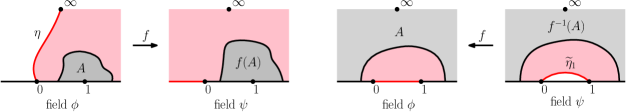
Figure 9: Left: Illustration for the proof of Lemma 5.6. Right: Illustration for the proof of Lemma 5.9.

By Proposition 5.3 and the definition of $M$, there is a constant $c$ such that the law of $(\psi,\mathcal{D})$ is $c\int\mathrm{LF}_{\mathbb{H}}^{(\gamma,0),(\beta_{2},1),(\beta_{2},\infty)}(\ell)\times{\mathcal{M}}^{\mathrm{disk}}_{2}(U;\ell)\,d\ell$, where $\mathrm{LF}_{\mathbb{H}}^{(\gamma,0),(\beta_{2},1),(\beta_{2},\infty)}(\ell)(d\psi)$ is defined as the disintegration of the measure $\mathrm{LF}_{\mathbb{H}}^{(\gamma,0),(\beta_{2},1),(\beta_{2},\infty)}(d\psi)$ on the event $\{\nu_{\psi}(-\infty,0)=\ell\}$.

Since $\eta$ is the interface when $(\mathbb{H},\psi,0,1,\infty)/{\sim_{\gamma}}$ is conformally welded to $\mathcal{D}$, the curve $\eta$ is measurable with respect to $\sigma(\mathcal{D},\nu_{\psi}|_{(-\infty,0)})$, thus $E:=\{\eta\subset\mathbb{H}\backslash A\}\in\sigma(\mathcal{D},\nu_{\psi}|_{(-\infty,0)})$. On $E$, define $S=f(A)$, and on $E^{c}$, define $S=\emptyset$. Lemma 5.4 is applicable with this choice of $S$. Consequently, conditioned on $E$ and on $(\mathcal{D},\psi|_{\mathbb{H}\backslash f(A)})$, we have $\psi|_{f(A)}\stackrel{{\scriptstyle d}}{{=}}\widetilde{h}+\widetilde{\mathfrak{h}}+\frac{\beta_{2}}{2}G_{f(A)}(\cdot,1)$, where $\widetilde{h}$ is a GFF on $f(A)$ with zero (resp. free) boundary conditions on $\partial f(A)\cap\mathbb{H}$ (resp. $\partial f(A)\cap\mathbb{R}$) and $\widetilde{\mathfrak{h}}$ is the harmonic extension of $\psi|_{\mathbb{H}\backslash f(A)}$ to $f(A)$ having normal derivative zero on $\partial(f(A))\cap\mathbb{R}$. By conformal invariance, we conclude that conditioned on $E$ and on $(\phi|_{\mathbb{H}\backslash A},\eta)$, we have $\phi|_{A}\stackrel{{\scriptstyle d}}{{=}}h+\mathfrak{h}+\frac{\beta_{2}}{2}G_{A}(\cdot,1)$.

Finally, since $(\phi,\eta)\sim M\times\mathrm{SLE}_{\kappa}(U-2;0,W-2)$, and the event $E$ only depends on $\eta$, we deduce the Markov property for $\phi$. ∎

Lemma 5.7.

Let $A\subset\mathbb{H}$ be a bounded neighborhood of $0$ such that $A$ and $\mathbb{H}\backslash A$ are simply connected and $\overline{A}\cap[1,\infty)=\emptyset$. For $\phi\sim M$, conditioned on $\phi|_{\mathbb{H}\backslash A}$ we have $\phi|_{A}\stackrel{{\scriptstyle d}}{{=}}h+\mathfrak{h}+\frac{\beta_{1}}{2}G_{A}(\cdot,0)$ where $h$ is a mixed boundary GFF in $A$ with zero (resp. free) boundary conditions on $\partial A\cap\mathbb{H}$ (resp. $\partial A\cap\mathbb{R}$), $\mathfrak{h}$ is the harmonic extension of $\phi|_{\mathbb{H}\backslash A}$ to $A$ with normal derivative zero on $\partial A\cap\mathbb{R}$, and $G_{A}$ is the Green function describing the covariance of $h$.

Proof.

Define $\eta_{2}$ as in the argument of Proposition 5.3. The same argument as in Lemma 5.6 applied to $(\phi,\eta_{2})$ yields the result. Indeed, the picture is symmetric if we interchange $U$ and $W-2$. ∎

Before proving the last Markov property Lemma 5.9, we first introduce a weighted quantum disk measure $\widetilde{\mathcal{M}}_{2}^{\mathrm{disk}}(U)$; this is not strictly necessary but simplifies the later exposition.

Lemma 5.8.

For $U\in(0,2]$ and $p\in(-1,\frac{4}{\gamma^{2}})$, if we sample a quantum disk from $R^{p}{\mathcal{M}}^{\mathrm{disk}}_{2}(U)$ then the law of $L$ is $1_{\ell>0}c\ell^{-\frac{2U}{\gamma^{2}}+p}\,d\ell$ where $c\in(0,\infty)$; here $L$ and $R$ are the left and right boundary arc lengths of the quantum disk. In particular, for $U<2$ the law of the left boundary arc length of $\widetilde{\mathcal{M}}^{\mathrm{disk}}_{2}(U):=R^{\frac{2U}{\gamma^{2}}}{\mathcal{M}}^{\mathrm{disk}}_{2}(U)$ is $c1_{\ell>0}\,d\ell$ for some $c\in(0,\infty)$.

Proof.

The exponent $-\frac{2U}{\gamma^{2}}+p$ is immediate from [AHS20, Lemma 2.19]; the interesting thing here is the fact that $c\in(0,\infty)$. If $U=2$ then this is immediate from the joint law $c(\ell+r)^{-\frac{4}{\gamma^{2}}-1}\,d\ell\,dr$ for $(L,R)$, where $c<\infty$ is a constant, see e.g. [AHS20, Proposition 7.8]. For $U<2$, this follows from the $U=2$ result and the fact that conformally welding a weight $U$ disk to a weight $(2-U)$ disk gives a weight 2 disk (Theorem 4.2). ∎

Lemma 5.9.

Let $A\subset\mathbb{H}$ be a neighborhood of $\infty$ such that $A$ and $\mathbb{H}\backslash A$ are simply connected and $\overline{A}\cap[0,1]=\emptyset$. For $\phi\sim M$, conditioned on $\phi|_{\mathbb{H}\backslash A}$ we have $\phi|_{A}\stackrel{{\scriptstyle d}}{{=}}h+\mathfrak{h}+(\frac{\beta_{3}}{2}-Q)G_{A}(\cdot,\infty)$ where $h$ is a mixed boundary GFF in $A$ with zero (resp. free) boundary conditions on $\partial A\cap\mathbb{H}$ (resp. $\partial A\cap\mathbb{R}$), $\mathfrak{h}$ is the harmonic extension of $\phi|_{\mathbb{H}\backslash A}$ to $A$ with normal derivative zero on $\partial A\cap\mathbb{R}$, and $G_{A}$ is the Green function describing the covariance of $h$.

Proof.

Let $\mathsf{m}(W;U)$ be the probability measure on pairs of curves from Theorem 4.1. Reflect this pair of curves across the line $\mathrm{Re}\,z=\frac{1}{2}$ to get a pair $(\widetilde{\eta}_{1},\widetilde{\eta}_{2})$ where $\widetilde{\eta}_{1}$ joins $0$ and $1$ and $\widetilde{\eta}_{2}$ joins $0$ and $\infty$. Let $\widetilde{\mathsf{m}}(W;U)$ be the law of $(\widetilde{\eta}_{1},\widetilde{\eta}_{2})$.

Let $\alpha=\gamma-\frac{2U}{\gamma}$. Sample

$$(\psi,\widetilde{\eta}_{1},\widetilde{\eta}_{2})\sim\nu_{\psi}(0,1)^{\frac{2U}{\gamma^{2}}}\mathrm{LF}_{\mathbb{H}}^{(\alpha,0),(\beta_{3},1)(\beta_{3},\infty)}(d\psi)\times\widetilde{\mathsf{m}}(W;U).$$

See Figure 9. By Theorem 4.1, the decorated quantum surface $(\mathbb{H},\psi,\widetilde{\eta}_{1},\widetilde{\eta}_{2},0,1,\infty)/{\sim_{\gamma}}$ has law

$$\iint_{0}^{\infty}\mathrm{Weld}({\mathcal{M}}^{\mathrm{disk}}_{2}(U;\ell),\mathrm{QT}(W,W,2;\ell;\ell^{\prime}),\widetilde{\mathcal{M}}^{\mathrm{disk}}_{2}(U;\ell^{\prime}))\,d\ell\,d\ell^{\prime},$$

where $\widetilde{\mathcal{M}}^{\mathrm{disk}}_{2}(U)$ is the weighted quantum disk defined in Lemma 5.8 and $\widetilde{\mathcal{M}}^{\mathrm{disk}}_{2}(U;\ell^{\prime})$ its disintegration by the unweighted boundary arc length.

By Lemma 5.8 we have $|\widetilde{\mathcal{M}}^{\mathrm{disk}}_{2}(U;\ell^{\prime})|=c$ for all $\ell^{\prime}$ for some finite constant $c$, so the marginal law of the decorated quantum surface above $\widetilde{\eta}_{1}$ is $c\int_{0}^{\infty}\mathrm{Weld}({\mathcal{M}}^{\mathrm{disk}}_{2}(U;\ell),\mathrm{QT}(W,W,2;\ell))\,d\ell$. Let $f$ be the conformal map sending the connected component of $\mathbb{H}\backslash\widetilde{\eta}_{1}$ above $\widetilde{\eta}_{1}$ to $\mathbb{H}$ such that $f$ fixes $(0,1,\infty)$, and let $\phi=f\bullet_{\gamma}\psi$. Then the marginal law of $\phi$ is $cM$.

Let $S=f^{-1}(A)$. Since $S$ is measurable with respect to $\widetilde{\eta}_{2}$ and $\psi$ is independent of $\widetilde{\eta}_{2}$, Lemma 5.4 tells us that conditioned on $S$ and $\psi|_{\mathbb{H}\backslash S}$, we have $\psi|_{S}\stackrel{{\scriptstyle d}}{{=}}h+\mathfrak{h}+(\frac{\beta_{3}}{2}-Q)G_{S}(\cdot,\infty)$ where $h$ is a GFF on $S$ with zero (resp. free) boundary conditions on $\partial S\cap\mathbb{H}$ (resp. $\partial S\cap\mathbb{R}$) and $\mathfrak{h}$ is the harmonic extension of $\psi|_{\mathbb{H}\backslash S}$ to $S$ with normal derivative zero on $\partial S\cap\mathbb{R}$. By the conformal invariance of the GFF and $\phi=f\bullet_{\gamma}\psi$, we obtain the desired Markov property for $\phi$. ∎

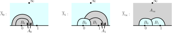
Figure 10: Illustration for the proof of Proposition 5.12. Each figure describes a Markov kernel where we resample the field in the grey region conditioned on the field in the blue region.

Lemma 5.10.

The measure $M$ is $\sigma$-finite.

Proof.

Let $V_{1},\dots,V_{n}\in(0,2]$ satisfy $\sum_{i=1}^{n}V_{i}=W-2$. Sample $(\eta,\eta_{2})\sim P_{U,W}$ (defined in the proof of Proposition 5.3), then in the region to the right of $\eta_{2}$ sample curves $(\hat{\eta}_{1},\dots,\hat{\eta}_{n-1})\sim\mathcal{P}^{\mathrm{disk}}(V_{1},\dots,V_{n})$ where $P^{\mathrm{disk}}(V_{1},\dots,V_{n})$ is the measure defined before Theorem 4.2. Let $\mathcal{L}$ denote the law of $(\eta,\eta_{2},\hat{\eta}_{1},\dots,\hat{\eta}_{n-1})$.

Sample $(\phi,\eta,\eta_{2},\hat{\eta}_{1},\dots,\hat{\eta}_{n-1})\sim M\times\mathcal{L}$, then the argument of Proposition 5.3 gives that the quantum surface $(\mathbb{H},\phi,\eta,\eta_{2},0,1,\infty)/{\sim_{\gamma}}$ has law (5.1). Applying Theorem 4.2, we see that the law of the quantum surface $(\mathbb{H},\phi,\eta,\eta_{2},\hat{\eta}_{1},\dots,\hat{\eta}_{n-1},0,1,\infty)/{\sim_{\gamma}}$ is

$$C^{\prime}\iiint_{0}^{\infty}\mathrm{Weld}({\mathcal{M}}^{\mathrm{disk}}_{2}(U;\ell),\mathrm{QT}(2,2,2;\ell,\ell^{\prime}),{\mathcal{M}}^{\mathrm{disk}}_{2}(V_{1};\ell^{\prime},\ell_{1}),\dots,{\mathcal{M}}^{\mathrm{disk}}_{2}(V_{n};\ell_{n-2},\ell_{n-1}))\,d\ell\,d\ell^{\prime}\,d\ell_{1}\dots d\ell_{n-1}.$$

Thus, for any $N>0$ the event $E_{N}$ that the quantum lengths of $\eta,\eta_{2},\hat{\eta}_{1},\dots,\hat{\eta}_{n-1}$ all lie in $(\frac{1}{N},N)$ has finite measure with respect to $M\times\mathcal{L}$, and the events $\{E_{N}\}_{N\geq 0}$ exhaust the sample space. Thus $M\times\mathcal{L}$ is $\sigma$-finite.

We now show that $M$ is $\sigma$-finite. Let $F_{N}$ be the set of $\phi$ such that conditioned on $\phi$, the conditional probability of $E_{N}$ is at least $\frac{1}{N}$. Then

$$\infty>(M\times\mathcal{L})[E_{N}]\geq\frac{1}{N}M[F_{N}],$$

so $M[F_{N}]<\infty$. Since $\{E_{N}\}_{N\geq 0}$ exhaust the sample space, the events $\{F_{N}\}$ also exhaust the sample space. ∎

We say a Markov kernel $K:\Omega\to\mathcal{F}$ on a measurable space $(\Omega,\mathcal{F})$ is irreducible if there exists a measure $\rho$ such that for any $A\in\mathcal{F}$ with $\rho(A)>0$ we have $K^{n}(\omega,A)>0$ for some $n>0$. [MT09, Propositions 4.2.1 and 10.1.1, Theorem 10.0.1] states that irreducible Markov chains with invariant probability measures have unique invariant probability measures. We need a $\sigma$-finite variant of this result.

Lemma 5.11.

Suppose a Markov kernel $K:\Omega\to\mathcal{F}$ on a measurable space $(\Omega,\mathcal{F})$ has two $\sigma$-finite invariant measures $\mu_{1},\mu_{2}$ such that for every $\omega\in\Omega$ the measures $\mu_{1},\mu_{2}$ are absolutely continuous with respect to $K(\omega,-)$. Further assume that for $i=1,2$ we have $K(x,dy)\mu_{i}(dx)=K(y,dx)\mu_{i}(dy)$. Then $\mu_{1}=c\mu_{2}$ for some $c\in(0,\infty)$.

Proof.

Let $E\in\mathcal{F}$ satisfy $\mu_{1}[E],\mu_{2}[E]<\infty$. Define the reflected Markov kernel $K_{E}(x,A):=K(x,A\cap E)+1_{x\in A}K(x,A\backslash E)$, i.e. if a step of a random walk would leave $E$ it instead stays in place. By reversibility, the measures $\mu_{1}|_{E}$ and $\mu_{2}|_{E}$ are invariant under $K_{E}$. Moreover $\mu_{1}|_{E}$ and $\mu_{2}|_{E}$ are absolutely continuous with respect to $K_{E}(\omega,-)$ for all $\omega\in E$, thus $K_{E}$ is irreducible. By [MT09, Propositions 4.2.1 and 10.1.1, Theorem 10.0.1] we have $\mu_{1}|_{E}=c\mu_{2}|_{E}$ for some constant $c$, and sending $E\uparrow\Omega$ gives the full result. ∎

Proposition 5.12.

Theorem 5.1 holds for $W>2$.

Proof.

Let $M$ be the law of the field $\phi$, then Proposition 5.3 identifies the law of $(\phi,\eta)$ as $M\times\mathrm{SLE}_{\kappa}(U-2;0,W-2)$. Thus it suffices to show that $M$ agrees with a multiple of $M^{\prime}:=\mathrm{LF}_{\mathbb{H}}^{(\beta_{1},0),(\beta_{2},1),(\beta_{3},\infty)}$.

We define three Markov transition kernels $\overline{\Lambda}_{0}$, $\overline{\Lambda}_{1}$ and $\overline{\Lambda}_{2}$ such that $M$ and $M^{\prime}$ are invariant measures under each Markov kernel, see Figure 10. Let $B_{0}\subset A_{0}$ be bounded neighborhoods of $0$ in $\mathbb{H}$ such that $\overline{A}_{0}\cap[1,\infty)=\emptyset$. Let $B_{1}\subset A_{1}$ be bounded neighborhoods of $1$ in $\mathbb{H}\backslash B_{0}$ such that $\overline{A}_{1}\cap(-\infty,0]=\emptyset$ and $\overline{B}_{1}\cap\partial B_{0}\neq\emptyset$. Finally let $A_{\infty}=\mathbb{H}\backslash\overline{B_{0}\cap B_{1}}$.

For $z\in\{0,1,\infty\}$, let $\overline{\Lambda}_{z}(\phi,d\psi)$ be the law of $\psi$ defined via $\psi|_{\mathbb{H}\backslash A_{z}}=\phi|_{\mathbb{H}\backslash A_{z}}$ and $\psi|_{A_{z}}=h+\mathfrak{h}+\frac{\alpha_{z}}{2}G_{A_{z}}(\cdot,z)$ where $h$ is a GFF in $A_{z}$, $\mathfrak{h}$ is the harmonic extension of $\phi|_{\mathbb{H}\backslash A_{z}}$ to $A_{z}$ having zero normal derivative on $\partial A_{z}\cap\mathbb{R}$, and $(\alpha_{0},\alpha_{1},\alpha_{\infty})=(\beta_{1},\beta_{2},\beta_{3}-2Q)$. By Lemmas 5.4, 5.6, 5.7 and 5.9, the measures $M$ and $M^{\prime}$ are invariant under $\overline{\Lambda}_{0},\overline{\Lambda}_{1}$ and $\overline{\Lambda}_{\infty}$, and more strongly we get reversibility: we have $\overline{\Lambda}_{j}(x,dy)M(dx)=\overline{\Lambda}_{j}(y,dx)M(dy)$ for $j\in\{0,1,\infty\}$, and the same holds for $M^{\prime}$.

Let $\widetilde{K}(\phi,dz)=\iint\overline{\Lambda}_{\infty}(y,dz)\overline{\Lambda}_{1}(x,dy)\overline{\Lambda}_{0}(\phi,dx)$, then $M$ and $M^{\prime}$ are invariant measures of $\widetilde{K}$. We now check that $M^{\prime}$ is absolutely continuous with respect to $\widetilde{K}(\phi,-)$ for all $\phi$. It is well known that if $h$ is a GFF in $A_{0}$ with zero (resp. free) boundary conditions on $\partial A_{0}\cap\mathbb{H}$ (resp. $\partial A_{0}\cap\mathbb{R}$) and $g$ is a smooth function on $A_{0}$, then the laws of $h|_{B_{0}}$ and $(h+g)|_{B_{0}}$ are mutually absolutely continuous, see e.g. the argument of [MS17, Proposition 2.9]. Thus, the $M^{\prime}(d\psi)$-law of $\psi|_{B_{0}}$ is absolutely continuous with respect to the $\overline{\Lambda}_{0}(\phi,dx)$-law of $x|_{B_{0}}$. Similarly, the $M^{\prime}(d\psi)$-law of $\psi|_{\overline{B_{0}\cup B_{1}}}$ is absolutely continuous with respect to the $\int\overline{\Lambda}_{1}(x,dy)\overline{\Lambda}_{0}(\phi,dx)$-law of $y|_{\overline{B_{0}\cup B_{1}}}$, and finally, $M^{\prime}$ is absolutely continuous with respect to $\iint\overline{\Lambda}_{\infty}(y,-)\overline{\Lambda}_{1}(x,dy)\overline{\Lambda}_{0}(\phi,dx)M(d\phi)$.

Now, let $K(\phi,dz)=\iint\overline{\Lambda}_{0}(y,dz)\overline{\Lambda}_{1}(x,dy)\widetilde{K}(\phi,dx)$. The measure $M^{\prime}$ is absolutely continuous with respect to $\widetilde{K}(\phi,-)$, and hence $K(\phi,-)$, for all $\phi$. Moreover, since $K=\overline{\Lambda}_{0}\overline{\Lambda}_{1}\overline{\Lambda}_{\infty}\overline{\Lambda}_{1}\overline{\Lambda}_{0}$, we get reversibility. Finally, $M$ is $\sigma$-finite (Lemma 5.10), and so is $M^{\prime}$ since the event $F_{N}$ that the average of $\psi$ on $(\partial B_{1}(0))\cap\mathbb{H}$ lies in $[-N,N]$ is finite satisfies $M^{\prime}[F_{N}]<\infty$, and $\{F_{N}\}_{N\geq 0}$ exhaust the sample space. By Lemma 5.11 $M=cM^{\prime}$ for some constant $c$, as desired. ∎

5.2 The case $W\in(\frac{\gamma^{2}}{2},2)$

The case $W\in(\frac{\gamma^{2}}{2},2)$ will be handled with the same proof structure as the $W>2$ case discussed in Section 5.1. The first step is to prove that the field and curve are independent, and identify the curve (Proposition 5.14). To that end, we need the following conformal welding result.

Lemma 5.13.

Let $U\in(0,2)$, $V\in(0,2-\frac{\gamma^{2}}{2})$ and $W=2-V$. Let $\widetilde{P}_{U,V}$ be the law of the curves $(\eta_{1},\eta_{2})$ in Figure 4 with parameters $(a_{1},a_{2},a_{3})=(\lambda(1-U),\lambda,\lambda)$ and $(\theta_{1},\theta_{2})=(0,\frac{\lambda(V-2)}{\chi})$. Sample

$$(\psi,\eta_{1},\eta_{2})\sim\mathrm{LF}_{\mathbb{H}}^{(\beta_{1},0),(\gamma,1),(\beta_{1},\infty)}\times\widetilde{P}_{U,V}.$$

Then the decorated quantum surface $(\mathbb{H},\psi,\eta_{1},\eta_{2},0,1,\infty)/{\sim_{\gamma}}$ has law

$$C\iint_{0}^{\infty}\mathrm{Weld}({\mathcal{M}}^{\mathrm{disk}}_{2}(U;\ell),\mathrm{QT}(W,2,W;\ell,\ell^{\prime}),{\mathcal{M}}^{\mathrm{disk}}_{2}(V;\ell^{\prime}))\,d\ell\,d\ell^{\prime},\qquad C\in(0,\infty).$$

Proof.

By [AHS21, Lemma 4.4], we have

$$\int_{0}^{\infty}\mathrm{Weld}(\mathrm{QT}(W,2,W;\ell^{\prime}),{\mathcal{M}}^{\mathrm{disk}}_{2}(V;\ell^{\prime}))\,d\ell^{\prime}=C_{1}\mathrm{QT}(2,2,2)\otimes\mathrm{SLE}_{\kappa}(-V;V-2),\qquad C_{1}\in(0,\infty).$$

By Proposition 5.2, we have

$$\int_{0}^{\infty}\mathrm{Weld}({\mathcal{M}}^{\mathrm{disk}}_{2}(U;\ell),\mathrm{QT}(2,2,2;\ell))\,d\ell=C_{2}\mathrm{QT}(U+2,U+2,2)\otimes\mathrm{SLE}_{\kappa}(U-2;0),\qquad C_{2}\in(0,\infty).$$

Combining these yields the result. ∎

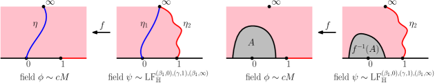
Figure 11: Left: Illustration for the proof of Proposition 5.14. Right: Illustration for the proof of Lemma 5.15.

Proposition 5.14.

In the setting of Theorem 5.1 with $W\in(\frac{\gamma^{2}}{2},2)$, let $M$ be the law of the field $\phi$. Then the joint law of $(\phi,\eta)$ is $M\times\mathrm{SLE}_{\kappa}(U-2;0,W-2)$.

Proof.

Let $V=2-W$. Recall the law $\widetilde{P}_{U,V}$ of Lemma 5.13. The marginal law of $\eta_{1}$ is $\mathrm{SLE}_{\kappa}(U-2;0)$ in $(\mathbb{H},0,\infty)$, and the conditional law of $\eta_{2}$ given $\eta_{1}$ is $\mathrm{SLE}_{\kappa}(-V;V-2)$ in $(D_{2},1,\infty)$ where $D_{2}$ is the connected component of $\mathbb{H}\backslash\eta_{1}$ with $1$ on its boundary.

Let $(\beta_{1},\beta_{2},\beta_{3})$ be insertions corresponding to weights $(2+U,2-V,2+U-V)$. Sample

$$(\psi,\eta_{1},\eta_{2})\sim\nu_{\psi}(1,\infty)^{\frac{2V}{\gamma^{2}}}\mathrm{LF}_{\mathbb{H}}^{(\beta_{1},0),(\gamma,1),(\beta_{1},\infty)}(d\psi)\times\widetilde{P}_{U,V}.$$

See Figure 11. By Lemma 5.13, the decorated quantum surface $(\mathbb{H},\psi,\eta_{1},\eta_{2},0,1,\infty)/{\sim_{\gamma}}$ has law

$$\iint_{0}^{\infty}\mathrm{Weld}({\mathcal{M}}^{\mathrm{disk}}_{2}(U;\ell),\mathrm{QT}(W,2,W;\ell,\ell^{\prime}),\widetilde{\mathcal{M}}^{\mathrm{disk}}_{2}(V;\ell^{\prime}))\,d\ell\,d\ell^{\prime},$$

where $\widetilde{\mathcal{M}}^{\mathrm{disk}}(V)$ is the weighted quantum disk defined in Lemma 5.8, and $\widetilde{\mathcal{M}}^{\mathrm{disk}}(V;\ell^{\prime})$ is the disintegration of $\widetilde{\mathcal{M}}^{\mathrm{disk}}(V)$ by the unweighted boundary arc length.

By Lemma 5.8 we have $|\widetilde{\mathcal{M}}^{\mathrm{disk}}_{2}(V;\ell)|=c$ for some finite constant $c$, so the marginal law of the decorated quantum surface to the left of $\eta_{2}$ is $c\int_{0}^{\infty}\mathrm{Weld}({\mathcal{M}}^{\mathrm{disk}}_{2}(U;\ell),\mathrm{QT}(W,2,W;\ell))\,d\ell$. Let $f$ be the conformal map sending the connected component of $\mathbb{H}\backslash\eta_{2}$ to the left of $\eta_{2}$ to $\mathbb{H}$ such that $f$ fixes $(0,1,\infty)$, and let $\phi=f\bullet_{\gamma}\psi$ and $\eta=f(\eta_{1})$. Then the marginal law of $\phi$ is $cM$.

Finally, by Proposition 3.1, when $(\eta_{1},\eta_{2})\sim\widetilde{P}_{U,V}$, the conditional law of $\eta_{1}$ given $\eta_{2}$ is $\mathrm{SLE}_{\kappa}(U-2;0,-V)$ the region to the left of $\eta_{2}$. Since $f$ is measurable with respect to $\sigma_{2}$, we deduce that the law of $(\phi,\eta)$ decomposes as a product measure $cM\times\mathrm{SLE}_{\kappa}(U-2;0,-V)$, as desired. ∎

Lemma 5.15.

For the measure $M$ defined in Proposition 5.14, the statements of Lemmas 5.6, 5.7 and 5.9 hold with $\beta_{1}=Q+\frac{\gamma}{2}-\frac{2+U}{\gamma}$, $\beta_{2}=Q+\frac{\gamma}{2}-\frac{W}{\gamma}$ and $\beta_{3}=Q+\frac{\gamma}{2}-\frac{U+W}{\gamma}$.

Proof.

The analogues of Lemmas 5.6 and 5.9 have exactly the same proofs as the original lemmas. We now discuss the analogue of Lemma 5.7.

The argument is very similar to that of Lemma 5.9 so we will be brief. We work in the setting of the argument of Proposition 5.14, see Figure 11. Let $A^{\prime}=f^{-1}(A)$, then since $f$ is measurable with respect to $\eta_{2}$ and $\psi$ is independent of $\eta_{2}$, the Markov property of the Liouville field gives a Markov property for $\psi|_{A^{\prime}}$ given $\psi|_{\mathbb{H}\backslash A^{\prime}}$. Using the map $f$, this gives the Markov property for $\phi_{A}$ given $\phi|_{\mathbb{H}\backslash A}$. ∎

Lemma 5.16.

$M$ is $\sigma$-finite.

Proof.

For $(\phi,\eta)\sim M\times\mathrm{SLE}_{\kappa}(U-2;0,W-2)$, the law of $(\mathbb{H},\phi,\eta,0,1,\infty)/{\sim_{\gamma}}$ is

$$c\int_{0}^{\infty}\mathrm{Weld}({\mathcal{M}}^{\mathrm{disk}}_{2}(U;\ell),\mathrm{QT}(W,2,W;\ell))\,d\ell\quad\text{ where }c\text{ is a constant},$$

so the event $E_{N}$ that the quantum length of $\eta$ lies in $[\frac{1}{N},N]$ has finite measure, and the events $\{E_{N}\}_{N\geq 0}$ exhaust the sample space. The rest of the argument is the same as that of Lemma 5.10. ∎

Proposition 5.17.

Theorem 5.1 holds for $W\in(\frac{\gamma^{2}}{2},2)$.

Proof.

The argument is identical to that of Proposition 5.12. We can define Markov kernels $\overline{\Lambda}_{z}(\phi,d\psi)$ for $z\in\{0,1,\infty\}$, under which $M$ and $M^{\prime}:=\mathrm{LF}_{\mathbb{H}}^{(\beta_{1},0),(\beta_{2},1),(\beta_{3},\infty)}$ are invariant by Lemmas 5.4 and 5.15. We then define the Markov kernel $K=\overline{\Lambda}_{0}\overline{\Lambda}_{1}\overline{\Lambda}_{\infty}\overline{\Lambda}_{1}\overline{\Lambda}_{0}$; it has $M$ and $M^{\prime}$ as invariant measures, and by the argument of Proposition 5.12 $K$ is irreducible. Finally, $M$ is $\sigma$-finite by Lemma 5.16, and $M^{\prime}$ is $\sigma$-finite by the same argument of Proposition 5.12, so Lemma 5.11 yields $M=cM^{\prime}$ for some constant $c$. ∎

6 Proof of Theorem 1.2 in the full range

In this section we prove Theorem 1.2. The first three subsections aim to establish the following weaker version of Theorem 1.2.

Let $\mathsf{m}$ be a measure on the space of curves in $(\mathbb{H},0,1,\infty)$ from $0$ to $\infty$ which do not hit $1$. Let $W,W_{1},W_{2},W_{3}>0$ such that none of $W+W_{1},W+W_{2},W_{1},W_{2},W_{3}$ equal $\frac{\gamma^{2}}{2}$. Sample a pair $S,\eta$ from $\mathrm{QT}(W+W_{1},W+W_{2},W+W_{3})\times\mathsf{m}$, let $(D,a_{1},a_{2},a_{3})$ be an embedding of $S$ and let $(\tilde{D},\tilde{a}_{1},\tilde{a}_{2},\tilde{a}_{3})$ be the corresponding embedding of the core of $S$. If $a_{1}\neq\tilde{a}_{1}$ let $\eta_{1}$ be independent $\mathrm{SLE}_{\kappa}(W-2;W_{1}-2)$ in each component in the interior of $D$ from $\tilde{a}_{1}$ to $a_{1}$. Likewise if $a_{2}\neq\tilde{a}_{2}$ let $\eta_{2}$ be independent $\mathrm{SLE}_{\kappa}(W-2;W_{2}-2)$ in each component in the interior of $D$ from $a_{2}$ to $\tilde{a}_{2}$. Let $\tilde{\eta}\subset D$ be the image of $\eta$ under the conformal map sending $\mathbb{H}$ to $(\tilde{D},\tilde{a}_{2},\tilde{a}_{3},\tilde{a}_{1})$, and let $\eta^{\prime}$ be the concatenation of $\tilde{\eta}$ with whichever of $\eta_{2},\eta_{1}$ we have defined. Let $\mathrm{QT}(W+W_{1},W+W_{2},{W}_{3})\otimes\mathsf{m}(W;W_{1},W_{2},W_{3})$ be the law of the decorated quantum surface $(D,\phi,a_{1},a_{2},a_{3},\eta^{\prime})$.

Proposition 6.1.

There exists a measure $\mathsf{m}(W;W_{1},W_{2},W_{3})$ and a constant $c=c_{W,W_{1},W_{2}}\in(0,\infty)$ such that

$$\mathrm{QT}(W+W_{1},W+W_{2},{W}_{3})\otimes\mathsf{m}(W;W_{1},W_{2},W_{3})=c\int_{0}^{\infty}\mathrm{Weld}({\mathcal{M}}^{\mathrm{disk}}_{2}(W;\ell),\mathrm{QT}(W_{1},W_{2},{W}_{3};\ell))d\ell$$ (6.1)

where we are welding the right boundary arc of the weight $W$ quantum disk with the left boundary arc of the quantum triangle linking the weight $W_{1}$ and $W_{2}$ vertices.

In particular, Theorem 5.1 is the special case of Proposition 6.1 with $W\in(0,\frac{\gamma^{2}}{2})$, $W_{1}=W_{3}>\frac{\gamma^{2}}{2}$ and $W_{2}=2$. In Section 6.1, by a reweighting argument, we are going to repeatedly apply Theorem 5.1 and hence prove Proposition 6.1 in the case where $W_{1},W_{2}>\frac{\gamma^{2}}{2}$ and $W,W_{3}>0$. In Section 6.2, we build on this result and work on the special case where $W_{1}+W_{2}={\gamma^{2}}$ using the thick-thin duality. Based on this, in Section 6.3 we conclude the proof of Proposition 6.1, while in Section 6.4 we identify the law of the curves via the SLE resampling property and thus complete the proof of Theorem 1.2 when none of the weights $W_{1},W_{2},W+W_{1},W+W_{2},W_{3}$ equal $\frac{\gamma^{2}}{2}$. Finally in Section 6.5 we prove the full version of Theorem 1.2 which addresses the case when some weight equals $\frac{\gamma^{2}}{2}$, while in Section 6.6 we prove Theorem 1.3 by a quick application of Theorem 1.2.

6.1 The $W_{1},W_{2}>\frac{\gamma^{2}}{2}$ regime

This section serves to prove the following:

Proposition 6.2.

Fix $W_{1},W_{2}>\frac{\gamma^{2}}{2}$ and $W,W_{3}>0$. Then there exists some measure $\mathsf{m}(W;W_{1},W_{2},W_{3})$ such that (6.1) holds.

To start with, we extend the idea of changing the weight of the third point as in [AHS21, Proposition 4.5] (See also Section 4.1) to quantum triangles with general weights in Proposition 6.3. Although this section only requires $W_{1},W_{2}>\frac{\gamma^{2}}{2}$, we state and prove Proposition 6.3 for a larger range for later sections. Suppose we have a curve-decorated surface from $\mathrm{QT}(W+W_{1},W+W_{2},\tilde{W}_{3})\otimes\mathsf{m}(W;W_{1},W_{2},\tilde{W}_{3})$ embedded as $(D,\phi,\eta,a_{1},a_{2},a_{3})$ and $\eta$ is a curve from $a_{2}$ to $a_{1}$. We choose $D$ such that each component of the interior of $D$ has smooth boundary. Let $(\tilde{D},\tilde{a}_{1},\tilde{a}_{2},\tilde{a}_{3})$ be the corresponding embedding of the core of the quantum triangle, and let $\tilde{D}_{\eta}$ be the connected component of $\tilde{D}\backslash\eta$ with $\tilde{a}_{3}$ on its boundary. See Figure 12. Let $\psi_{\eta}:\tilde{D}_{\eta}\to\mathbb{H}$ be the conformal mapping sending the first (resp. last) point on $\partial D_{\eta}$ (resp. $\partial D$) hit by $\eta$ to 0 (resp. $\infty$) and sending $\tilde{a}_{3}$ to $1$, and $\psi:\tilde{D}\to\mathbb{H}$ be the conformal map sending $(\tilde{a}_{2},\tilde{a}_{1},\tilde{a}_{3})$ to $(0,\infty,1)$.

Proposition 6.3.

Suppose that given $W,W_{1},W_{2},W_{3},\tilde{W}_{3}>0$, $W_{3},\tilde{W}_{3}\neq\frac{\gamma^{2}}{2}$ with $W_{1},W_{2},W+W_{1},W+W_{2}\neq\frac{\gamma^{2}}{2}$, there exists some measure $\mathsf{m}(W;W_{1},W_{2},\tilde{W}_{3})$ on random simple curves in $D$ starting from $a_{2}$ to $a_{1}$ and not hitting $a_{3}$ such that we have the conformal welding of quantum triangles as in (6.1) with $W_{3}$ replaced by $\tilde{W}_{3}$. Then if we define the measure $\mathsf{m}(W;W_{1},W_{2},W_{3})$ on curves by setting

$$\frac{d\mathsf{m}(W;W_{1},W_{2},W_{3})}{d\mathsf{m}(W;W_{1},W_{2},\tilde{W}_{3})}(\eta)=\left|\frac{\psi^{\prime}_{\eta}(a_{3})}{\psi^{\prime}(a_{3})}\right|^{\Delta_{\widetilde{\beta}_{3}}-\Delta_{\beta_{3}}}$$

where $\beta_{3}=\gamma+\frac{2-W_{3}}{\gamma}$ and $\tilde{\beta_{3}}=\gamma+\frac{2-\tilde{W}_{3}}{\gamma}$. Then (6.1) holds.

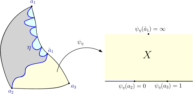
Figure 12: Setup of Proposition 6.3 in the case $W_{1}<\frac{\gamma^{2}}{2}$ and $W,W_{2},\tilde{W}_{3}>\frac{\gamma^{2}}{2}$ and an illustration of the conformal map $\psi_{\eta}$. By decorating a quantum triangle from $\mathrm{QT}(W+W_{1},W+W_{2},\tilde{W}_{3})$ with an independent curve $\eta$ from $\mathsf{m}(W;W_{1},W_{2},\tilde{W}_{3})$ we get a weight $W$ disk $S_{1}$ (gray) and a quantum triangle with weights $W_{1},W_{2},\tilde{W}_{3}$, which has two parts $S_{2}$ (blue) and $S_{3}$ (yellow). Consider the conformal map $\psi_{\eta}$ and let $X$ be the corresponding surface embedded on $\mathbb{H}$ as on the right panel. Weighting the law of curve-decorated surface by $e^{(\beta_{3}-\tilde{\beta}_{3})X(1)}$ allows us to shift (6.1) to $W_{3}$ from the $\tilde{W}_{3}$ case.

We can define a disintegration $\mathrm{LF}_{\mathbb{H}}^{(\beta_{1},\infty),(\beta_{2},0),(\beta_{3},1)}=\int_{0}^{\infty}\mathrm{LF}_{\mathbb{H},\ell}^{(\beta_{1},\infty),(\beta_{2},0),(\beta_{3},1)}\,d\ell$ where for each $\ell>0$ the measure $\mathrm{LF}_{\mathbb{H},\ell}^{(\beta_{1},\infty),(\beta_{2},0),(\beta_{3},1)}$ is supported on $\{\nu_{\phi}((-\infty,0))=\ell\}$, see e.g. Definition 2.26 and Lemma 2.27.

Lemma 6.4.

Let $\beta_{1},\beta_{2}<Q$, $\beta_{3},\tilde{\beta}_{3}\in\mathbb{R}$ and $\ell>0$. In the sense of weak convergence of measures,

$$\lim_{\varepsilon\to 0}\varepsilon^{\frac{\beta_{3}^{2}-\tilde{\beta}_{3}^{2}}{4}}e^{\frac{\beta_{3}-\tilde{\beta}_{3}}{2}\phi_{\varepsilon}(1)}\mathrm{LF}_{\mathbb{H},\ell}^{(\beta_{1},\infty),(\beta_{2},0),(\tilde{\beta}_{3},1)}(d\phi)=\mathrm{LF}_{\mathbb{H},\ell}^{(\beta_{1},\infty),(\beta_{2},0),({\beta}_{3},1)}(d\phi).$$ (6.2)

The proof is identical to that of [AHS21, Lemma 4.6], which is a direct application of the Girsanov theorem. We omit the details.

Proof of Proposition 6.3.

We first note that if the result holds for $W_{3},\tilde{W}_{3}>\frac{\gamma^{2}}{2}$, then it holds for the full range $W_{3},\tilde{W}_{3}\in(0,\infty)\backslash\{\frac{\gamma^{2}}{2}\}$. Indeed, if $W_{3}<\frac{\gamma^{2}}{2}<\tilde{W}_{3}$, we can use Proposition 6.3 with $W_{3}$ replaced by $\gamma^{2}-W_{3}$ and concatenate a weight $W_{3}$ quantum disk to the weight $\gamma^{2}-W_{3}$ vertex; since $\Delta_{\beta}$ takes the same value for $\beta=\gamma+\frac{2-W_{3}}{\gamma}$ and $\beta=\gamma+\frac{2-(\gamma^{2}-W_{3})}{\gamma}$, the law of the curve is as desired. For $W_{3}$ arbitrary and $\tilde{W}_{3}<\frac{\gamma^{2}}{2}$, recall that the quantum triangle with weights $(W_{1},W_{2},\tilde{W}_{3})$ is obtained by concatenating a quantum triangle with weights $(W_{1},W_{2},\gamma^{2}-\tilde{W}_{3})$ and a quantum disk of weight $W_{3}$; by forgetting this quantum disk we reduce the problem to the solved case where $\tilde{W}_{3}$ is replaced by $\gamma^{2}-\tilde{W}_{3}$. Henceforth we assume $W_{3},\tilde{W}_{3}>\frac{\gamma^{2}}{2}$.

First assume $W_{1}+W,W_{2}+W>\frac{\gamma^{2}}{2}$. The quantum triangle from $\mathrm{QT}(W+W_{1},W+W_{2},\tilde{W}_{3})$ can be embedded as $c\mathrm{LF}_{\mathbb{H}}^{(\beta_{1},\infty),(\beta_{2},0),(\tilde{\beta}_{3},1)}$ with the random curve $\eta$ going from 0 to $\infty$ not hitting 1. Sample $(Y,\eta)$ from $c\mathrm{LF}_{\mathbb{H}}^{(\beta_{1},\infty),(\beta_{2},0),(\tilde{\beta}_{3},1)}\times\mathsf{m}(W;W_{1},W_{2},\tilde{W}_{3})$, so by definition $(\mathbb{H},Y,\eta,\infty,0,1)/{\sim_{\gamma}}$ has the law of the left hand side of (6.1) with $W_{3}$ replaced by $\tilde{W}_{3}$. Let $D_{\eta}^{1}$ be the union of the components of $\mathbb{H}\backslash\eta$ whose boundaries contain a segment of $(-\infty,0)$, $D_{\eta}^{3}$ be the component of $\mathbb{H}\backslash\eta$ with 1 on its boundary as defined, and $D_{\eta}^{2}$ be the union of the remaining components (if not empty). Set

$$X=Y\circ\psi_{\eta}^{-1}+Q\log|(\psi_{\eta}^{-1})^{\prime}|$$ (6.3)

and define the quantum surfaces $S_{1}=(D_{\eta}^{1},Y,\infty,0)/{\sim_{\gamma}}$, $S_{2}=(D_{\eta}^{2},Y)/\sim_{\gamma}$, $S_{3}=(\mathbb{H},X,\infty,0,1)/\sim_{\gamma}$. See also Figure 12 for the setup. By (6.1) for $\tilde{W}_{3}$ instead of $W_{3}$ and our definition of quantum triangles, $S_{2}$ and $S_{3}$ are independent, while the conditional law of $S_{1}$ given $(S_{2},S_{3})$ is ${\mathcal{M}}^{\mathrm{disk}}_{2}(W;L)$ where $L$ is $\nu_{X}((-\infty,0))$ plus the sum of the quantum lengths of boundary arcs of $S_{2}$ lying within $\mathbb{H}$. We weight the law of $(Y,\eta)$ by $\varepsilon^{\frac{\beta_{3}^{2}-\tilde{\beta}_{3}^{2}}{4}}e^{\frac{\beta_{3}-\tilde{\beta}_{3}}{2}X_{\varepsilon}(1)}$ and send $\varepsilon\to 0$; using the argument of [AHS21, Proposition 4.5], the conditional law of $S_{1}$ given the pair $(S_{2},S_{3})$ is unchanged. Moreover, by the independence of $S_{2}$ and $S_{3}$, by Lemma 6.4, $(S_{2},S_{3})$ converges in law to $c\mathrm{QT}(W_{1},W_{2},W_{3})$ under the reweighting as $\varepsilon\to 0$, the joint law of the quantum surfaces $(S_{1},S_{2},S_{3})$ converges to the right hand side of (6.1), while the law of $(Y,\eta)/{\sim_{\gamma}}$ converges to the left side of (6.1). This finishes the proof for the case $W_{1}+W,W_{2}+W>\frac{\gamma^{2}}{2}$.

For the case where $W_{i}+W<\frac{\gamma^{2}}{2}$ for some $i$, we apply the above argument to the core of the quantum triangle; the proof is then identical. ∎

Proof of Proposition 6.2.

Step 1. $W\in(0,\frac{\gamma^{2}}{2})$, $W_{1}>\frac{\gamma^{2}}{2}$ and $W_{2}\geq 2$. First assume $W_{2}\in[2,\frac{\gamma^{2}}{2}+2)$. We start from the weight $(W_{1},2,2)$ triangle and weld an independent quantum disk from ${\mathcal{M}}^{\mathrm{disk}}_{2}(W)$ to its left boundary and an independent disk from ${\mathcal{M}}^{\mathrm{disk}}_{2}(W_{2}-2)$ to its bottom arc, see Figure 13. That is, we work on the measure

$$\int_{0}^{\infty}\int_{0}^{\infty}\mathrm{Weld}({\mathcal{M}}^{\mathrm{disk}}_{2}(W;\ell),\mathrm{QT}(W_{1},2,2;\ell,s),{\mathcal{M}}^{\mathrm{disk}}_{2}(W_{2}-2;s))dsd\ell.$$ (6.4)

On one hand, if we fix $s$ and integrate over $\ell$ first, i.e., we weld together the quantum triangle and the weight $W$ quantum disk, by Theorem 5.1 and Proposition 6.3, (6.4) is a constant multiple of

$$\int_{0}^{\infty}\mathrm{Weld}\bigg{(}\big{(}\mathrm{QT}(W+2,2,W+W_{1};s)\otimes\mathsf{m}(W;W_{1},2,2)\big{)},{\mathcal{M}}^{\mathrm{disk}}_{2}(W_{2}-2;s)\bigg{)}ds.$$ (6.5)

Integrating over $s$, by Theorem 5.1 we see that (6.5) is a constant times

$$\mathrm{QT}(W+W_{1},W+W_{2},W_{2})\otimes\mathsf{m}_{2}$$ (6.6)

where $\mathsf{m}_{2}$ is some measure on tuple of curves $(\eta_{1},\eta_{2})$, such that $\eta_{2}$ has marginal law $\mathsf{m}(W_{2}-2;W+2,2,W+W_{1})$ in $\mathbb{H}$ from 1 to 0 and the conditional law of $\eta_{2}$ given $\eta_{1}$ is $\mathsf{m}(W;W_{1},2,2)$ in $\mathbb{H}\backslash\eta_{2}$ from $0$ to $\infty$.

On the other hand, if we fix $\ell$ and integrate over $s$ first, i.e., we weld together the quantum triangle and the weight $W_{2}-\gamma^{2}+W_{1}$ quantum disk, by (4.5), we get a constant times

$$\int_{0}^{\infty}\mathrm{Weld}\bigg{(}{\mathcal{M}}^{\mathrm{disk}}_{2}(W;\ell),\big{(}\mathrm{QT}(W_{1},W_{2},W_{2})\otimes\mathsf{m}(W_{2}-2;2,2,W_{1})\big{)}\bigg{)}d\ell.$$ (6.7)

Therefore if we forget about the curve $\eta_{2}$ and compare (6.6) with (6.7), we obtain (6.1) in case $W_{3}=\tilde{W}_{3}:=W_{2}$. Applying Proposition 6.3 once more yields (6.1) for $W\in(0,\frac{\gamma^{2}}{2})$, $W_{1}>\frac{\gamma^{2}}{2}$ and $W_{2}{=W_{3}}\in[2,\frac{\gamma^{2}}{2}+2)$. Proposition 6.3 then allows us to choose $W_{3}$ arbitrary, completing the proof in this case.

Now suppose we have proved (6.1) for $W\in(0,\frac{\gamma^{2}}{2})$, $W_{1}>\frac{\gamma^{2}}{2}$ and $W_{2}\in[2+\frac{k\gamma^{2}}{2},2+\frac{(k+1)\gamma^{2}}{2})$ and some $k\geq 0$. Then for $W_{2}\in[2+\frac{(k+1)\gamma^{2}}{2},2+\frac{(k+2)\gamma^{2}}{2})$ we pick $U<\frac{\gamma^{2}}{2}$ such that $W_{2}\in[2+\frac{k\gamma^{2}}{2},2+\frac{(k+1)\gamma^{2}}{2})$, and replace the the weight $(W_{1},2,2)$ triangle in  (6.4) with a weight $(W_{1},W_{2}-U,W_{2}-U)$ quantum triangle and the weight $W_{2}-2$ quantum disk with a weight $U$ quantum disk. Then (6.1) follows by precisely the same argument and our assumption. This finishes the induction, so Step 1 is complete.

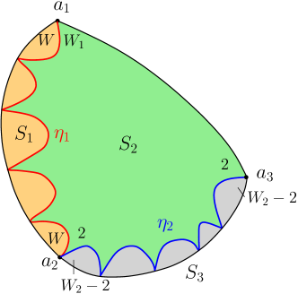
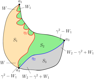
Figure 13: Left: Step 1 of proof of Proposition 6.2. We consider the simultaneous welding of the weight $W$ quantum disk (surface $S_{1}$), weight $(W_{1},2,2)$ quantum triangle (surface $S_{2}$) and weight $W_{2}-2$ quantum disk (surface $S_{3}$). If we choose to weld $S_{1}$ with $S_{2}$ first then $S_{3}$, we get a quantum triangle of weight $(W+W_{1},W+W_{2},W_{2})$ decorated with independent curves $(\eta_{1},\eta_{2})$. On the other hand, if we weld $S_{2}$ with $S_{3}$ first, we obtain a quantum triangle of weight $(W_{1},W_{2},W_{2})$ decorated by curve $\eta_{2}$. Thus we conclude that by further welding a weight $W$ quantum disk to the left and forgetting about $\eta_{2}$ we get a quantum triangle of weight $(W+W_{1},W+W_{2},W_{2})$ decorated by an independent curve $\eta_{1}$. Right: Step 1 for Proposition 6.1. The proof is almost identical and only the weights has been changed.

Step 2: $W>0$ and $\max\{W_{1},W_{2}\}\geq 2$. By symmetry we may assume $W_{2}\geq 2$. Suppose (6.1) holds for $W\in[\frac{k\gamma^{2}}{2},\frac{(k+1)\gamma^{2}}{2})$, $W_{1}>\frac{\gamma^{2}}{2}$ and $W_{2}\geq 2$ where again $k\geq 0$ is an integer. Note that the case $k=0$ follows directly from Step 1. Now if $W\in[\frac{(k+1)\gamma^{2}}{2},\frac{(k+2)\gamma^{2}}{2})$, again we pick some $U\in(0,\frac{\gamma^{2}}{2})$ such that $W-U\in[\frac{k\gamma^{2}}{2},\frac{(k+1)\gamma^{2}}{2})$. We start with a weight $(W_{1},W_{2},W_{3})$ quantum triangle. We first glue a weight $U$ quantum disk on its left boundary, inducing an interface $\eta_{2}$, and then a weight $W_{1}-U$ quantum disk to the left. That is, we are working with the measure

$$\int_{0}^{\infty}\int_{0}^{\infty}\mathrm{Weld}({\mathcal{M}}^{\mathrm{disk}}_{2}(W-U;\ell),{\mathcal{M}}^{\mathrm{disk}}_{2}(U;\ell,s),\mathrm{QT}(W_{1},W_{2},W_{3};s))dsd\ell.$$ (6.8)

See Figure 14 (left). Again by Step 1, we can now integrate over $s$ first and weld the weight $U$ quantum disk with the quantum triangle, with the law of the curve-decorated surface being $\mathrm{QT}(W_{1}+U,W_{2}+U,W_{3};\ell)\otimes\mathsf{m}(U;W_{1},W_{2},W_{3})$. Then by our induction hypothesis, integrating over $\ell$ once more and welding in the weight $(W-U)$ quantum disk, we obtain a quantum triangle of weight $(W+W_{1},W+W_{2},W_{3})$ decorated by independent curves $(\eta_{1},\eta_{2})$. On the other hand, if we weld the two disks first, by Theorem 4.2, we get

$$\int_{0}^{\infty}\mathrm{Weld}\bigg{(}\big{(}{\mathcal{M}}^{\mathrm{disk}}_{2}(W;\ell)\otimes\mathrm{SLE}_{\kappa}(W-U-2;U-2)\big{)},\mathrm{QT}(W_{1},W_{2},W_{3};\ell)\bigg{)}d\ell.$$ (6.9)

Thus if we forget about the curve $\eta_{1}$ and treat $\eta_{2}$ as the interface, we obtain (6.1). This finishes the induction step and draws the conclusion.

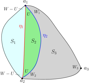
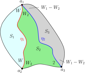
Figure 14: Left: Step 2 of proof of Proposition 6.2. Applying Step 1 and our induction hypothesis we can first weld $S_{3}$ to the right of $S_{2}$ and $S_{1}$ to the left to get a quantum triangle of weight $(W+W_{1},W+W_{2},W_{3})$. If we forget about $\eta_{1}$ then we get the left hand side of (6.1). On the other hand by Theorem 4.2 we can first weld $S_{1}$ and $S_{2}$ and the picture becomes the right hand side of (6.1). Right: The same commutation argument in Step 3.

Step 3: The general $W>0,W_{1},W_{2}>\frac{\gamma^{2}}{2}$ case. By symmetry and Step 2, we may assume $\frac{\gamma^{2}}{2}<W_{2}<W_{1}\leq 2$. We consider the setting of the right panel of Figure 14. Again by comparing the procedure of first welding $S_{2}$ with $S_{1}$ (by (4.5)) and then $S_{3}$ (by Step 2; and we obtain a quantum triangle with weight $(W+W_{1},W+W_{2},W_{1}-W_{2}+2)$) and first welding $S_{2}$ with $S_{3}$ (by Step 3 and we get a quantum triangle of weight $(W_{1},W_{2},W_{1}-W_{2}+2)$) and then $S_{1}$, we obtain (6.1) with $W_{3}=W_{1}-W_{2}+2$. Thus we conclude the proof by Proposition 6.3. ∎

6.2 The $W_{1}+W_{2}=\gamma^{2}$ regime via thick-thin duality

Let $W\in(0,\frac{\gamma^{2}}{2})$. In this section, we establish the conformal welding of a quantum triangle of weights $W,\gamma^{2}-W,2$ with a thick quantum disk, via Theorem 6.5. The key observation is that, using the thick-thin duality, the concatenation point on the quantum triangle has weight $2+\gamma^{2}$ in the global field and hence the $\beta$-value for insertion becomes $\beta=\gamma+\frac{2-(2+\gamma^{2})}{\gamma}=0$.

Theorem 6.5.

Fix $W>\frac{\gamma^{2}}{2}$, $W_{1}\in(0,\frac{\gamma^{2}}{2})$ and $W_{2}=\gamma^{2}-W_{1}$. Embed a sample from $\mathrm{QT}(W+W_{1},W+W_{2},2)$ as $(\mathbb{H},\phi,\infty,0,1)$, where the points $(\infty,0,1)$ corresponds to the weights $(W+W_{1},W+W_{2},2)$. Then there exists some constant $c=c_{W,W_{1}}\in(0,\infty)$ and some measure $\mathsf{m}(W;W_{1},W_{2},2)$ on random curves in $\mathbb{H}$ from $0$ to $\infty$ avoiding 1, such that

$$\begin{split}\mathrm{QT}(W+W_{1},W+W_{2},2)\otimes\mathsf{m}(W;W_{1},W_{2},2)=c\int_{0}^{\infty}\mathrm{Weld}({\mathcal{M}}^{\mathrm{disk}}_{2}(W;\ell),\mathrm{QT}(W_{1},W_{2},2;\ell))d\ell.\end{split}$$ (6.10)

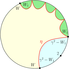
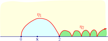
Figure 15: Left: Setup of Theorem 6.5, where we are proving that cutting a triangle from $\mathrm{QT}(W+W_{1},W+\gamma^{2}-W_{1},2)$ with some independent curve $\eta$ from $\mathsf{m}(W,W_{1},\gamma^{2}-W_{1},2)$ yields the welding of an independent weight $W$ disk and a thin triangle from $\mathrm{QT}(W_{1},\gamma^{2}-W_{1},2)$. Right: Conclusion of Lemma 6.6, embedded as $(\mathbb{H},\phi,\eta,\infty,0,2)$. We sample a point $\mathbf{x}$ from the quantum length measure on $[0,2]$ and use the scaling $f_{\mathbf{x}}(z)=\frac{z}{\mathbf{x}}$ to put the added point at 1.

By definition, the quantum surface on the right hand side of (6.10) consists of three parts: a weight $W$ two-pointed quantum disk, a weight $W_{1}$ thin quantum disk, and a three-pointed quantum disk from ${\mathcal{M}}^{\mathrm{disk}}_{2,\bullet}(W_{2})$. These can be glued together by Proposition 6.2. Parallel to our definition of thin quantum triangles, let $\tilde{\mathcal{M}}_{2}(W_{1})$ be the law of the quantum surface obtained by concatenating a sample from ${\mathcal{M}}^{\mathrm{disk}}_{2}(W_{1})\times{\mathcal{M}}^{\mathrm{disk}}_{2}(W_{2})$ with $W_{2}=\gamma^{2}-W_{1}$. Then we have the disintegration on the left boundary length

$$\tilde{\mathcal{M}}_{2}(W_{1};\ell)=\int_{0}^{r}{\mathcal{M}}^{\mathrm{disk}}_{2}(W_{1};r)\times{\mathcal{M}}^{\mathrm{disk}}_{2}(W_{2};\ell-r)dr.$$ (6.11)

Lemma 6.6.

In the setting of Theorem 6.5, there exists some constant $c=c_{W,W_{1}}\in(0,\infty)$ such that

$$\mathrm{QT}(W+W_{1},W+\gamma^{2}-W_{1},\gamma^{2}+2)\otimes\tilde{\mathsf{m}}(W,W_{1})=c\int_{0}^{\infty}\mathrm{Weld}({\mathcal{M}}^{\mathrm{disk}}_{2}(W;\ell),\tilde{\mathcal{M}}_{2}(W_{1};\ell))d\ell$$ (6.12)

where $\tilde{\mathsf{m}}(W,W_{1})$ is some law on pairs of the curves describing the two interfaces.

Proof.

We start with a triply marked quantum disk sampled from ${\mathcal{M}}^{\mathrm{disk}}_{2,\bullet}(W)$ and recall that ${\mathcal{M}}^{\mathrm{disk}}_{2,\bullet}(W)$ is a constant multiple of $\mathrm{QT}(W,W,2)$ (see Remark 2.19). By applying Proposition 6.2 twice, we can simultaneously glue quantum disks with weight $W_{1}$ and $\gamma^{2}-W_{1}$ to the marked boundary of the ${\mathcal{M}}^{\mathrm{disk}}_{2,\bullet}(W)$ quantum disk, with interface having law $\tilde{\mathsf{m}}(W,W_{1})$ and being independent of the surface. That is, if we write ${\mathcal{M}}^{\mathrm{disk}}_{2,\bullet}(W;\ell,r)$ for disintegration of the measure ${\mathcal{M}}^{\mathrm{disk}}_{2,\bullet}(W)$ over the length of the two boundary arcs containing the third marked point, then

$$\begin{split}&\mathrm{QT}(W+W_{1},W+\gamma^{2}-W_{1},\gamma^{2}+2)\otimes\tilde{\mathsf{m}}(W,W_{1})\\ &=c\int_{0}^{\infty}\int_{0}^{\infty}\mathrm{Weld}({\mathcal{M}}^{\mathrm{disk}}_{2,\bullet}(W;r,\ell),{\mathcal{M}}^{\mathrm{disk}}_{2}(W_{1};r),{\mathcal{M}}^{\mathrm{disk}}_{2}(\gamma^{2}-W_{1};\ell))d\ell dr\\ &=c\int_{0}^{\infty}\int_{0}^{\ell}\mathrm{Weld}({\mathcal{M}}^{\mathrm{disk}}_{2,\bullet}(W;r,\ell-r),{\mathcal{M}}^{\mathrm{disk}}_{2}(W_{1};r),{\mathcal{M}}^{\mathrm{disk}}_{2}(\gamma^{2}-W_{1};\ell-r))drd\ell.\end{split}$$ (6.13)

Now we study the right hand side of (6.13). By Definition 2.13, forgetting the marked point of a sample from ${\mathcal{M}}^{\mathrm{disk}}_{2,\bullet}(W;r,\ell-r)$ gives a sample from ${\mathcal{M}}^{\mathrm{disk}}_{2}(W;\ell)$. Combining this with (6.11), we conclude that the right hand side of (6.13) equals that of (6.12). ∎

Proof of Theorem 6.5.

We begin with the setting of Lemma 6.6. Embed the quantum triangle from $\mathrm{QT}(W+W_{1},W+\gamma^{2}-W_{1},\gamma^{2}+2)$ as $(\mathbb{H},\phi,\infty,0,2)$. The law of $\phi$ is $c\mathrm{LF}_{\mathbb{H}}^{(\beta_{1},\infty),(\beta_{2},0)}$ where $\beta_{1}=\gamma+\frac{2-W-W_{1}}{\gamma}$, $\beta_{2}=\gamma+\frac{2-W-\gamma^{2}+W_{1}}{\gamma}$ and $c=c_{W,W_{1}}$ is some constant. We emphasize that there is no $\beta$-insertion at the marked point 2 since $\beta_{3}=\gamma+\frac{2-(2+\gamma^{2})}{\gamma}=0$. The interface $\eta_{1}$ between the weight $W$ quantum disk and the weight $\gamma^{2}-W_{1}$ quantum disk is embedded as a simple curve from 0 to 2, and the interface $\eta_{2}$ between the weight $W$ disk and the weight $W_{1}$ thin disk is drawn as a boundary hitting curve from 2 to $\infty$. See Figure 15 for an illustration of the setup.

We add a fourth point to the field and rescale via the following procedure. First weight the law of $\phi$ by $\nu_{\phi}([0,2])$ and sample a point $\mathbf{x}$ on $(0,2)$ from the probability measure proportional to the quantum length measure $\nu_{\phi}|_{[0,2]}$, and then rescale the field and the curves via $f_{\mathbf{x}}(z)=\frac{z}{\mathbf{x}}$. Let

$$\tilde{\phi}=f_{x}\bullet_{\gamma}\phi=\phi\circ f_{\mathbf{x}}^{-1}+Q\log|(f_{\mathbf{x}}^{-1})^{\prime}|=\phi(\mathbf{x}\cdot)+Q\log\mathbf{x}.$$ (6.14)

Then $(\mathbb{H},\tilde{\phi},\infty,0,1)/{\sim_{\gamma}}=(\mathbb{H},\phi,\infty,0,\mathbf{x})/{\sim_{\gamma}}$. Let $\eta$ be the concatenation of the curves $\mathbf{x}^{-1}\eta_{1}(\cdot)$ and $\mathbf{x}^{-1}\eta_{2}(\cdot)$, going from 0 to $\infty$. Note that this point $\mathbf{x}$ is added to the weight $\gamma^{2}-W_{1}$ disk according to quantum length measure, and again by Proposition 2.14 this surface has the same law as $c\mathrm{QT}(\gamma^{2}-W_{1},\gamma^{2}-W_{1},2)$. Therefore, by applying the definition of quantum triangles, the law of the curve-decorated surface $(\mathbb{H},\tilde{\phi},\eta,\infty,0,1)$ is precisely the same as the right hand side of (6.10). We are going to prove that $\tilde{\phi}$ has the same law as $\mathrm{LF}_{\mathbb{H}}^{(\beta_{1},\infty),(\beta_{2},0),(\gamma,1)}$ and is independent of $\mathbf{x}$, which further implies that $\eta$ is independent of $\tilde{\phi}$ (since $\eta$ is defined via $\eta_{1},\eta_{2},\mathbf{x}$, which are all independent of $\tilde{\phi}$). This shows that the law of $(\mathbb{H},\tilde{\phi},\eta,\infty,0,1)$ is the same as the left hand side of (6.10), which concludes the proof.

Now suppose that $F$ is a bounded, non-negative and continuous function on $H^{-1}(\mathbb{H})$, and $g$ is a compactly supported non-negative function on $[0,2]$. Let $\phi_{\varepsilon}(x)$ be the circle average of $\phi$ around the semicircle $\{z:|z-x|=\varepsilon\}$. By the change of coordinates (6.14), $(f_{x}\bullet_{\gamma}\phi)_{\frac{\varepsilon}{x}}(1)=\phi_{\varepsilon}(x)+Q\log x$. Let $Q(d\phi,dx)=\nu_{\phi}(dx)\mathrm{LF}_{\mathbb{H}}^{(\beta_{1},\infty),(\beta_{2},0)}(d\phi)$ be the infinite measure on $H^{-1}(\mathbb{H})\times[0,2]$. Then

$$\begin{split}Q[F(\tilde{\phi})g(\mathbf{x})]&=\lim_{\varepsilon\to 0}\int\int_{0}^{2}F(f_{x}\bullet_{\gamma}\phi)g(x)\varepsilon^{\frac{\gamma^{2}}{4}}e^{\frac{\gamma}{2}\phi_{\varepsilon}(x)}dx\mathrm{LF}_{\mathbb{H}}^{(\beta_{1},\infty),(\beta_{2},0)}(d\phi)\\ &=\lim_{\varepsilon\to 0}\int\int_{0}^{2}F(f_{x}\bullet_{\gamma}\phi)g(x)(\frac{\varepsilon}{x})^{\frac{\gamma^{2}}{4}}x^{\frac{\gamma^{2}}{4}}e^{\frac{\gamma}{2}(f_{x}\bullet_{\gamma}\phi)_{\frac{\varepsilon}{x}}(1)-\frac{\gamma}{2}Q\log x}dx\mathrm{LF}_{\mathbb{H}}^{(\beta_{1},\infty),(\beta_{2},0)}(d\phi)\\ &=\lim_{\varepsilon\to 0}\int\int_{0}^{2}F(f_{x}\bullet_{\gamma}\phi)g(x)\varepsilon^{\frac{\gamma^{2}}{4}}e^{\frac{\gamma}{2}(f_{x}\bullet_{\gamma}\phi)_{\varepsilon}(1)}x^{\frac{\gamma^{2}-2\gamma Q}{4}}dx\mathrm{LF}_{\mathbb{H}}^{(\beta_{1},\infty),(\beta_{2},0)}(d\phi)\\ &=\lim_{\varepsilon\to 0}\int_{0}^{2}\int F(\tilde{\phi})g(x)\varepsilon^{\frac{\gamma^{2}}{4}}e^{\frac{\gamma}{2}\tilde{\phi}_{\varepsilon}(1)}x^{\frac{\gamma^{2}-2\gamma Q}{4}}[(f_{x})_{*}\mathrm{LF}_{\mathbb{H}}^{(\beta_{1},\infty),(\beta_{2},0)}](d\tilde{\phi})dx.\end{split}$$ (6.15)

Here we have used the fact that $\lim_{\varepsilon\to 0}\int_{0}^{2}\varepsilon^{\frac{\gamma^{2}}{4}}e^{\frac{\gamma}{2}h_{\varepsilon}(x)}g(x)dx=\int_{0}^{2}g(x)\nu_{h}(dx)$ in $L^{1}$ with respect to $P_{\mathbb{H}}$ (see e.g. [Ber17, Theorem 1.1]). Meanwhile, by Lemma 2.7 and Lemma 2.10, we have

$$\begin{split}(f_{x})_{*}\mathrm{LF}_{\mathbb{H}}^{(\beta_{1},\infty),(\beta_{2},0)}&=\lim_{r\to+\infty}r^{2\Delta_{\beta_{1}}}(f_{x})_{*}\mathrm{LF}_{\mathbb{H}}^{(\beta_{1},r),(\beta_{2},0)}\\ &=\lim_{r\to+\infty}r^{2\Delta_{\beta_{1}}}x^{-\Delta_{\beta_{1}}-\Delta_{\beta_{2}}}\mathrm{LF}_{\mathbb{H}}^{(\beta_{1},\frac{r}{x}),(\beta_{2},0)}=x^{\Delta_{\beta_{1}}-\Delta_{\beta_{2}}}\mathrm{LF}_{\mathbb{H}}^{(\beta_{1},\infty),(\beta_{2},0)}.\end{split}$$ (6.16)

Since $\frac{\gamma^{2}-2\gamma Q}{4}=-1$, plugging (6.16) into (6.15) and using Lemma 2.6, we get

$$\begin{split}Q[F(\tilde{\phi})g(\mathbf{x})]&=\lim_{\varepsilon\to 0}\int_{0}^{2}\bigg{(}\int F(\tilde{\phi})\varepsilon^{\frac{\gamma^{2}}{4}}e^{\frac{\gamma}{2}\tilde{\phi}_{\varepsilon}(1)}\mathrm{LF}_{\mathbb{H}}^{(\beta_{1},\infty),(\beta_{2},0)}(d\tilde{\phi})\bigg{)}g(x)x^{-1+\Delta_{\beta_{1}}-\Delta_{\beta_{2}}}dx\\ &=\bigg{(}\int F(\tilde{\phi})\mathrm{LF}_{\mathbb{H}}^{(\beta_{1},\infty),(\beta_{2},0),(\gamma,1)}(d\tilde{\phi})\bigg{)}\bigg{(}\int_{0}^{2}g(x)x^{-1+\Delta_{\beta_{1}}-\Delta_{\beta_{2}}}dx\bigg{)}.\end{split}$$ (6.17)

Therefore the law of $\tilde{\phi}$ is $\mathrm{LF}_{\mathbb{H}}^{(\beta_{1},\infty),(\beta_{2},0),(\gamma,1)}$ and is independent of the choice of $\mathbf{x}$, which concludes our proof.

∎

6.3 Extension to general weights

In this section, we finish the proof of Proposition 6.1 by repeatedly applying the change of weight argument in Proposition 6.3 along with Theorem 6.5. Since most of the proof isn identical to that of Proposition 6.2, we will only list the welding pictures and explain by which theorem we can weld surfaces together.

Proof of Proposition 6.1.

Without loss of generality, we only need to focus on the case when a least one of $W_{1}$ and $W_{2}$ is in $(0,\frac{\gamma^{2}}{2})$.

Step 1: $W_{1}\in(0,\frac{\gamma^{2}}{2})$, $W\geq\frac{\gamma^{2}}{2}$, $W_{2}\geq\gamma^{2}-W_{1}$. Consider the setting on the right panel of Figure 13. We start from the weight $(W_{1},\gamma^{2}-W_{1},\gamma^{2}-W_{1})$ quantum triangle $S_{2}$ and weld an independent quantum disk $S_{1}$ from ${\mathcal{M}}^{\mathrm{disk}}_{2}(W)$ to its left boundary and an independent quantum disk $S_{3}$ from ${\mathcal{M}}^{\mathrm{disk}}_{2}(W_{2}-(\gamma^{2}-W_{1}))$ to its bottom arc. If we first weld $S_{1}$ to the left of $S_{2}$ (by Theorem 6.5) and then $S_{3}$ to the bottom (by Proposition 6.2) and forget about $\eta_{2}$, the resulting law of the curve-decorated surface is the left hand side of (6.1). Meanwhile, we can also start by welding $S_{2}$ and $S_{3}$ together, which (by Proposition 4.3) leads to the right hand side of (6.1). This justifies the claim.

Step 2: $W_{1}\in(0,\frac{\gamma^{2}}{2}),\ W>0,\ W_{2}\geq\gamma^{2}$. By Step 1 we can assume $W\in(0,\frac{\gamma^{2}}{2})$. Consider the welding on the left panel of Figure 16. By Proposition 4.3, we can first weld $S_{1}$ and $S_{2}$ together. Then we weld the disk $S_{3}$ from below (if $W_{1}+W<\frac{\gamma^{2}}{2}$ then this is covered by Step 1; otherwise this is from Proposition 6.2). However we can also apply Theorem 6.5 and Proposition 6.3 to glue $S_{2}$ and $S_{3}$ together first. Comparing the two procedures (and applying Proposition 6.3) yields (6.1). By symmetry we may also swap $W_{1}$ and $W_{2}$ and (6.1) holds for $W_{1}\geq\gamma^{2},\ W>0,\ W_{2}\in(0,\frac{\gamma^{2}}{2})$.

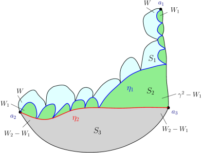
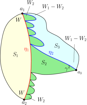
Figure 16: Left: Step 2 of the proof of Proposition 6.1. We can weld the three surfaces together by first glue $S_{1}$ with $S_{2}$ and then $S_{3}$ on the bottom. Apply this procedure we get a large triangle of weights $(W+W_{1},W+W_{2},W_{2}+\gamma^{2}-2W_{1})$. We can also weld $S_{2}$ with $S_{3}$ first and get a triangle of weights $(W_{1},W_{2},W_{2}+\gamma^{2}-2W_{1})$. Comparing the two procedures we get (6.1) (By Proposition 6.3, the weight at vertex $a_{3}$ can be replaced by any $W_{3}>0$). Right: Step 3 of Proposition 6.1. We can start by gluing $S_{1}$ and $S_{2}$ (Proposition 4.3) and then glue $S_{3}$ to the right (Proposition 6.2 and Step 2) to get a triangle of weights $(W+W_{1},W+W_{2},W_{1}-W_{2}+2)$ decorated with independent curves $(\eta_{1},\eta_{2})$. We can also start with $S_{2}$ and $S_{3}$ instead and see that the surface to the right of $\eta_{1}$ has law $\mathrm{QT}(W_{1},W_{2},W_{1}-W_{2}+2)$. Apply Proposition 6.3 once more we get the welding equation (6.1).

Step 3. The remaining cases. Without loss of generality suppose $W_{2}<W_{1}\leq\gamma^{2}$ and $W_{2}<\frac{\gamma^{2}}{2}$ (if $W_{1}=W_{2}$ then the claim is straightforward from Proposition 4.3). Consider a quantum triangle $S_{2}$ of weight ($W_{2},W_{2},\gamma^{2}$). Again by Proposition 4.3 we can weld a weight $W$ quantum disk $S_{1}$ to the left. Then we weld a weight $W_{1}-W_{2}$ quantum disk $S_{3}$ to the right and forget about the interface (if $W+W_{2}<\frac{\gamma^{2}}{2}$ we apply Step 2; otherwise we apply Proposition 6.2). Meanwhile we can apply Step 2 to weld $S_{2}$ and $S_{3}$ first. Comparing the two procedures (and change the third weight by Proposition 6.3) we obtain (6.1). ∎

6.4 The interface law

In this section, we identify the interface law $\mathsf{m}$ in Proposition 6.1 as $\widetilde{\mathrm{SLE}}_{\kappa}(W-2;W_{2}-2,W_{1}-W_{2},\alpha)$ with $\alpha=\frac{W_{3}+W_{2}-W_{1}-2}{4\kappa}(W_{3}+W_{1}+2-W_{2}-\kappa)$ using the SLE curve resampling properties, which completes the proof of Theorem 1.2 when none of the weights $W+W_{1},W+W_{2},W_{1},W_{2},W_{3}$ equals $\frac{\gamma^{2}}{2}$. We begin with the direct extension of Theorem 5.1 and work on the case where $W_{1}\geq W_{2}>0$, while the case $W_{2}>W_{1}$ is covered via the SLE${}_{\kappa}(\rho_{-};\rho_{+},\rho_{1})$ reversibility in Theorem 1.5. Note that if $W+W_{1}<\frac{\gamma^{2}}{2}$ and/or $W+W_{2}<\frac{\gamma^{2}}{2}$ then as in Proposition 3.1 and the discussion at the beginning of Section 6, the $\widetilde{\mathrm{SLE}}_{\kappa}(W-2;W_{2}-2,W_{1}-W_{2},\alpha)$ curve is understood as the concatenation of an $\widetilde{\mathrm{SLE}}_{\kappa}(W-2;W_{2}-2,W_{1}-W_{2},\alpha)$ in the core with independent $\mathrm{SLE}_{\kappa}(W-2;W_{1}-2)$ and/or $\mathrm{SLE}_{\kappa}(W-2;W_{2}-2)$ in each bead of the weight $W+W_{1}$ and/or $W+W_{2}$ thin quantum disk.

Lemma 6.7.

Suppose $W,W_{1}>0$ and $W_{1},W+W_{1}\neq\frac{\gamma^{2}}{2}$. Then there exists some constant $c=c_{W,W_{1}}\in(0,\infty)$ such that

$$\mathrm{QT}(W+W_{1},W+2,W_{1})\otimes\mathrm{SLE}_{\kappa}(W-2;0,W_{1}-2)=c\int_{0}^{\infty}\mathrm{Weld}({\mathcal{M}}^{\mathrm{disk}}_{2}(W;\ell),\mathrm{QT}(W_{1},2,{W}_{1};\ell))d\ell.$$ (6.18)

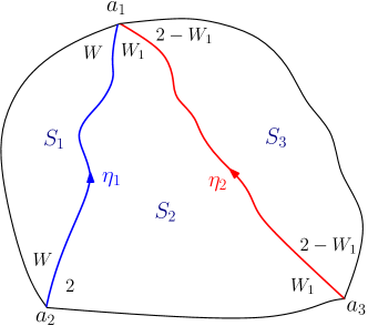
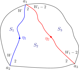
Figure 17: Left: Suppose $W_{1}<2$. Then we can weld a quantum disk of weight $2-W_{1}$ to the right side of the quantum triangle, as in the left panel. Conditioned on the surface $S_{1}$ and the interface $\eta_{1}$, Proposition 4.3 tells us that the interface $\eta_{2}$ has law $\mathrm{SLE}_{\kappa}(W_{1}-2;-W_{1})$ from $a_{3}$ to $a_{1}$ on the domain to the right of $\eta_{1}$, while the marginal law of $\eta_{1}$ is $\mathrm{SLE}_{\kappa}(W-2)$. This characterizes the law on pairs $(\eta_{1},\eta_{2})$, while one can verify by Proposition 3.1 that the right panel gives a desired coupling. Furthermore by Imaginary geometry the conditional law of $\eta_{1}$ given $\eta_{2}$ is $\mathrm{SLE}_{\kappa}(W-2;0,W_{1}-2)$, which justifies (6.18). Right: For $W_{1}>2$, similar to the left panel, by Proposition 4.3 the conditional law of $\eta_{1}$ given $\eta_{2}$ is $\mathrm{SLE}_{\kappa}(W-2)$, while the law of $\eta_{2}$ given $\eta_{1}$ is $\mathrm{SLE}_{\kappa}(W_{1}-4)$. Therefore by Proposition 3.1 the marginal law of $\eta_{1}$ is $\mathrm{SLE}_{\kappa}(W-2;0,W_{1}-2)$.

Proof.

If $W_{1}=2$, then the lemma follows directly from Proposition 4.3. For $W_{1}\neq 2$, see Figure 17 for an illustration. ∎

Now we deal with the case $W_{1}\geq W_{2}>0$. Recall the notion of $\widetilde{\mathrm{SLE}}_{\kappa}(\rho_{-};\rho_{+},\rho_{1};\alpha)$ in (1.6).

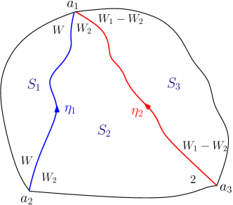
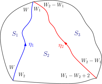
Figure 18: Left: Suppose $W+W_{2}\geq\frac{\gamma^{2}}{2}$. Again consider the welding of the three surfaces as in the left panel. Similar to the explanation in Figure 17, by Proposition 4.3 the conditional law of $\eta_{1}$ given $\eta_{2}$ is $\mathrm{SLE}_{\kappa}(W-2;W_{2}-2)$, while by Lemma 6.7, the marginal law of $\eta_{2}$ is $\mathrm{SLE}_{\kappa}(0,W+W_{2}-2;W_{1}-W_{2}-2)$. Therefore by Proposition 3.1 we can infer that the marginal law of $\eta_{1}$ is $\mathrm{SLE}_{\kappa}(W-2;W_{2}-2,W_{1}-W_{2})$, which gives (1.8). Right: Suppose $\max\{W_{1},W_{2}\}\geq 2$ and $|W_{1}-W_{2}|<2$. Consider the welding picture in the left panel. By Propositions 4.3 and 6.8 we may figure out the joint law of $(\eta_{1},\eta_{2})$ and therefore recover from Proposition 3.1 that the conditional law of $\eta_{1}$ given $\eta_{2}$ is $\mathrm{SLE}_{\kappa}(W-2;W_{2}-2,W_{1}-W_{2})$.

Proposition 6.8.

Theorem 1.2 holds when $W_{1}\geq W_{2}$ and $\frac{\gamma^{2}}{2}\not\in\{W+W_{1},W+W_{2},W_{1},W_{2},W_{3}\}$.

Proof.

Again if $W_{1}=W_{2}$ then the conclusion is clear from Proposition 4.3. Now we start with the case $W_{3}=W_{1}-W_{2}+2$ so that $\alpha=0$ and there is no weighting in the $\mathrm{SLE}$ law. The case when $W+W_{2}\geq\frac{\gamma^{2}}{2}$ is explained in Figure 18. If $W+W_{2}<\frac{\gamma^{2}}{2}$, then we may first replace $W$ with $\tilde{W}=2-W_{2}$ in Figure 18 and draw an independent curve $\eta_{0}\sim\mathrm{SLE}_{\kappa}(-W-W_{2};W-2)$ in the weight $\tilde{W}$ disk. Using the same argument one can read off the conditional law of $\eta_{1}$ given $\eta_{0}$, which coincides with that in (1.8). Finally for general $W_{3}>0$, we apply Proposition 6.3. In this setting, $\tilde{\beta}_{3}=\gamma+\frac{W_{2}-W_{1}}{\gamma}$ and $\beta_{3}=\gamma+\frac{2-W_{3}}{\gamma}$, and we finish the proof by calculating

$$\Delta_{\tilde{\beta}_{3}}-\Delta_{\beta_{3}}=\frac{W_{3}+W_{2}-W_{1}-2}{4\kappa}(W_{3}+W_{1}+2-W_{2}-\kappa)=\alpha.$$

∎

Proposition 6.8 has discussed the interface law for the case $W_{1}\geq W_{2}$. Now if $W_{1}<W_{2}$, by applying Theorem 1.5 and reversing the orientation of the curve, we are now able to finish the proof of Theorem 1.2 when none of the weights are $\frac{\gamma^{2}}{2}$.

Proposition 6.9.

Theorem 1.2 holds when $W_{1},W_{2},W_{3},W+W_{1},W+W_{2}\neq\frac{\gamma^{2}}{2}$.

Proof.

By Proposition 6.8, it remains to work on the case where $W_{1}<W_{2}$. Consider the welding as in the right hand side of (1.8) but with the interface going in the reverse direction. Then by Proposition 6.8 and left-right symmetry, the law of the interface is $\widetilde{\mathrm{SLE}}_{\kappa}(W_{1}-2,W_{2}-W_{1};W-2;\tilde{\alpha})$ where

$$\tilde{\alpha}=\frac{W_{3}+W_{1}-W_{2}-2}{4\kappa}(W_{3}+W_{2}+2-W_{1}-\kappa).$$

Note that the conformal radius appeared in the definition (1.6) is invariant under time reversal and the conformal map $z\mapsto-\frac{1}{z}$, therefore as we reverse the direction and let the interface $\eta$ go from $a_{2}$ to $a_{1}$, then by Theorem 1.5 $\eta$ has law $\widetilde{\mathrm{SLE}}_{\kappa}(W-2;W_{2}-2,W_{1}-W_{2};\tilde{\alpha}+\frac{(W_{2}-W_{1})(4-\kappa)}{2\kappa})$. (Again if any of $W+W_{1}$, $W+W_{2}$ is smaller than $\frac{\gamma^{2}}{2}$ then in each bead given by thin disk part we apply [MS16b, Theorem 1.1].) Therefore we conclude the proof by noticing $\tilde{\alpha}+\frac{(W_{2}-W_{1})(4-\kappa)}{2\kappa}=\alpha$ as given in (1.8). ∎

6.5 Welding of quantum triangles with weight $\frac{\gamma^{2}}{2}$

In this section, we finish the proof of Theorem 1.2. Using Proposition 6.9 and taking a limit, we can allow one or more of $W_{1},W_{2},W_{3}$ to be $\frac{\gamma^{2}}{2}$ and require $W>\frac{\gamma^{2}}{2}$ (Proposition 6.10). This argument is technical because we need to truncate on suitable events to make the measures finite. Finally we remove the remaining constraint $\frac{\gamma^{2}}{2}\not\in\{W+W_{1},W+W_{2}\}$ in Proposition 6.11 via gluing with an extra quantum disk.

Proposition 6.10.

Theorem 1.2 holds when $W+W_{1},W+W_{2}\neq\frac{\gamma^{2}}{2}$ and $W>\frac{\gamma^{2}}{2}$.

Proof.

We may assume that $W_{3}\geq\frac{\gamma^{2}}{2}$ since the $W_{3}<\frac{\gamma^{2}}{2}$ case follows from applying the result with the weight $\gamma^{2}-W_{3}$ and concatenating with a thin quantum disk of weight $W_{3}$.

We first explain the proof when $W_{1},W_{2}\geq\frac{\gamma^{2}}{2}$, then adapt the argument to the general case.

For each $i$ such that $W_{i}\neq\frac{\gamma^{2}}{2}$, let $(W_{i}^{n})$ be the constant sequence equal to $W_{i}$. For $i$ such that $W_{i}=\frac{\gamma^{2}}{2}$, let $(W_{i}^{n})$ be a decreasing sequence with limit $W_{i}$. Let $K>0$ be a parameter we will later send to $\infty$. Let $\rho$ be a probability measure with compact support in $\{z\in\mathcal{S}\>:\>|z|\leq 1/K\}$ such that $\iint G_{\mathcal{S}}(z,w)\rho(dw)\rho(dz)<\infty$.

Define the event $E_{K}$ for a pair of fields $X$ and $Y$ on $\mathcal{S}$:

$$E_{K}=\{\nu_{X}((-\infty,1)),\nu_{X}((1,\infty)),|(X,\rho)|,|(Y,\rho)|<K\}.$$

Let $x_{1}=+\infty,x_{2}=-\infty,x_{3}=1$, and let $\{\mathrm{LF}_{\mathcal{S},\ell}^{(\beta_{i}^{n},x_{i})_{i}}\}$ be the disintegration of $\mathrm{LF}_{\mathcal{S}}^{(\beta_{i}^{n},x_{i})_{i}}$ with respect to the quantum length of $\mathbb{R}\times\{\pi\}$, where $\beta_{i}^{n}:=Q+\frac{\gamma}{2}-\frac{W_{i}^{n}}{\gamma}$ for $i=1,2,3$. Sample $(X_{n},\mathcal{D}_{n})$ from $\int_{0}^{\infty}\mathrm{LF}_{\mathcal{S,\ell}}^{(\beta_{i}^{n},x_{i})_{i}}\times{\mathcal{M}}^{\mathrm{disk}}_{2}(W;\ell)\,d\ell$, and let $Y_{n}$ be the field such that $\mathcal{D}_{n}=(\mathcal{S},Y_{n},-\infty,+\infty)/{\sim_{\gamma}}$ and $\nu_{Y_{n}}(\mathbb{R})=\ell$ with embedding fixed by specifying $\nu_{Y_{n}}((-\infty,0)\times\{\pi\})=\nu_{Y_{n}}((0,\infty)\times\{\pi\})$. Let $\mathcal{L}_{n}$ be the law of $(X_{n},Y_{n})$. Similarly, sample $(X,Y)$ in the same way with $W_{i}^{n}$ replaced by $W_{i}$, and let $\mathcal{L}$ be the law of $(X,Y)$.

For a field $Z$ in $\mathcal{S}$ and a curve $\eta$ from $-\infty$ to $+\infty$ in $\mathcal{S}$ disjoint from $\partial\mathcal{S}$, define

$$X(Z,\eta)=f\bullet_{\gamma}Z,\qquad\qquad Y(Z,\eta)=g\bullet_{\gamma}Z$$

where $f$ is the conformal map from the connected component of $\mathcal{S}\backslash\eta$ below $\eta$ to $\mathcal{S}$ fixing $-\infty,+\infty$ and $1$, and $g$ is the conformal map from the connected component of $\mathcal{S}\backslash\eta$ above $\eta$ to $\mathcal{S}$ sending $(-\infty,+\infty,p)\mapsto(-\infty,+\infty,i\pi)$ where $p\in\mathbb{R}\times\{\pi\}$ is the point such that the $\nu_{Z}$-lengths of the two components of $(\mathbb{R}\times\{\pi\})\backslash\{p\}$ are the same. Let $\widetilde{E}_{K}$ be the event $\{(Z,\eta)\>:\>(X(Z,\eta),Y(Z,\eta))\in E_{K}\}$. In other words,

$$\widetilde{E}_{K}=\{(Z,\eta)\>:\>\nu_{Z}((-\infty,1)),\nu_{Z}((1,+\infty)),|(X(Z,\eta),\rho)|,|(Y(Z,\eta),\rho)|<K\}.$$

Let $\tilde{\beta}_{i}^{n}=Q+\frac{\gamma}{2}-\frac{W_{i}^{n}+W}{\gamma}$ for $i=1,2$ and let $\tilde{\beta}_{3}^{n}=\beta_{3}^{n}$. Let $\mathcal{L}_{n}^{\prime}$ be the law of a field and curve sampled from $\mathrm{LF}_{\mathcal{S}}^{(\tilde{\beta}_{i}^{n},x_{i})_{i}}\times\widetilde{\mathrm{SLE}}_{\kappa}(W-2;W_{2}^{n}-2,W_{1}^{n}-W_{2}^{n};\alpha)$ and conditioned on $\widetilde{E}_{K}$, and $\mathcal{L}^{\prime}$ the corresponding law when the $W_{i}^{n}$ are replaced by $W_{i}$ for $i=1,2,3$. We need to show that for a fixed $K$, if we sample $(Z,\eta)$ from $\mathcal{L}^{\prime}$, then the law of $(X(Z,\eta),Y(Z,\eta))$ is $\mathcal{L}$.

Let $F_{\varepsilon}=\{Z\>:\>|(Z,\rho)|<1/\varepsilon\}$ and $G_{\varepsilon}=\{\eta\>:\>\mathrm{dist}(1,\eta)>\varepsilon\}$. For fixed $\varepsilon$, as finite measures on the space of curves in $\mathcal{S}$ (equipped with the Gromov-Hausdorff topology for the two-point compactification of $\mathcal{S}$) we have $\lim_{n\to 0}\widetilde{\mathrm{SLE}}_{\kappa}(W-2;W_{2}^{n}-2,W_{1}^{n}-W_{2}^{n};\alpha)|_{G_{\varepsilon}}=\widetilde{\mathrm{SLE}}_{\kappa}(W-2;W_{2}-2,W_{1}-W_{2};\alpha)|_{G_{\varepsilon}}$. This and Proposition 2.32 imply that the measure $\mathcal{L}_{n}^{\prime}|_{F_{\varepsilon}\times G_{\varepsilon}}$ converges as $n\to\infty$ to $\mathcal{L}^{\prime}|_{F_{\varepsilon}\times G_{\varepsilon}}$.

By Proposition 6.9, for $(Z_{n},\eta_{n})\sim\mathcal{L}_{n}^{\prime}$, the law of $(X(Z_{n},\eta_{n}),Y(Z_{n},\eta_{n}))$ is $\mathcal{L}_{n}$, and by Proposition 2.32 we have $\mathcal{L}_{n}\to\mathcal{L}$. Combining this with $\mathcal{L}_{n}^{\prime}|_{F_{\varepsilon}\cap G_{\varepsilon}}\to\mathcal{L}^{\prime}|_{F_{\varepsilon}\cap G_{\varepsilon}}$ and $\mathcal{L}^{\prime}[F_{\varepsilon}\times G_{\varepsilon}]=1-o_{\varepsilon}(1)$, we conclude that for $(Z,\eta)\sim\mathcal{L}^{\prime}$ the law of $(X(Z,\eta),Y(Z,\eta))$ is within $o_{\varepsilon}(1)$ in total variation distance of $\mathcal{L}$. In fact, we see that the law is exactly $\mathcal{L}$ by sending $\varepsilon\to 0$. Finally, sending $K\to\infty$ gives the desired result for $W_{1},W_{2}\geq\frac{\gamma^{2}}{2}$.

For the general case where $W_{1},W_{2}$ might not both be thick, the argument is essentially identical, just that in various definitions we would have extra thin quantum disks (corresponding to the weights with $W_{i}<\frac{\gamma^{2}}{2}$). For instance, if $W_{1}<\frac{\gamma^{2}}{2}\leq W_{2},W_{3}$, we define $\mathcal{L}_{n}$ to be the law of $(X,Y,\mathcal{D}_{1})$ where we sample $(\mathcal{T},\mathcal{D})\sim\int_{0}^{\infty}\mathrm{QT}(W_{1}^{n},W_{2}^{n},W_{3}^{n};\ell)\times{\mathcal{M}}^{\mathrm{disk}}_{2}(W;\ell)\,d\ell$, let $Y$ and $X$ be the fields in $\mathcal{S}$ from suitably embedding $\mathcal{D}$ and the core of $\mathcal{T}$, let $\mathcal{D}_{1}$ be the (weight $W_{1}$) thin quantum disk at the first vertex of $\mathcal{T}$, and condition on the event $E_{K}$ that the two sides of $\mathcal{T}$ adjacent to the weight $W_{3}$ vertex have quantum lengths at most $K$ and $|(X,\rho)|,|(Y,\rho)|<K$. We similarly modify the definitions of $\mathcal{L},\mathcal{L}^{\prime}_{n},\mathcal{L}^{\prime}$; the arguments are otherwise identical. ∎

Proposition 6.11.

Theorem 1.2 holds.

Proof.

See Figure 19. We start by sampling

$$(\mathcal{D}^{\prime},\mathcal{D},\mathcal{T})\sim\iint_{0}^{\infty}{\mathcal{M}}^{\mathrm{disk}}_{2}(2;\ell_{1})\times\,{\mathcal{M}}^{\mathrm{disk}}_{2}(W;\ell_{1},\ell_{2})\times\,\mathrm{QT}(W_{1},W_{2},W_{3};\ell_{2})\,d\ell_{1}\,d\ell_{2}.$$ (6.19)

By Theorem 4.2, we can weld $\mathcal{D}^{\prime}$ to $\mathcal{D}$ first and then apply Proposition 6.10 to weld $\mathcal{T}$ in. As a consequence,  (6.19) is a constant multiple of $\mathrm{QT}(W_{1}+W+2,W_{2}+W+2,W_{3})\otimes\mathfrak{m}$, where $\mathfrak{m}$ is some measure on the interfaces $(\eta_{1},\eta_{2})$. If we embed the entire surface as $(\mathbb{H},\infty,0,1)$, then $(\eta_{1},\eta_{2})$ can be produced by (i) sample $\eta_{2}$ as a curve from 0 to $\infty$ from $\widetilde{\mathrm{SLE}}_{\kappa}(W;W_{2}-2,W_{1}-W_{2};\alpha)$ with $\alpha$ given by (1.7) and force points $0^{-};0^{+},1$ and (ii) sample $\eta_{1}$ on the left component of $\mathbb{H}\backslash\eta_{2}$ from the measure $\mathrm{SLE}_{\kappa}(0;W-2)$ with force points $0^{-};0^{+}$. Then by Lemma 3.3, we know that a sample $(\eta_{1},\eta_{2})\sim\mathfrak{m}$ can also be obtained by (i) sample $\eta_{1}$ from $\widetilde{\mathrm{SLE}}_{\kappa}(0;W_{2}-2,W_{1}-W_{2};\alpha)$ with force points $0^{-};0^{+},1$ and (ii) sample $\eta_{2}$ on the right component of $\mathbb{H}\backslash\eta_{1}$ from $\widetilde{\mathrm{SLE}}_{\kappa}(W-2;W_{2}-2,W_{1}-W_{2};\alpha)$ with force points $0^{-};0^{+},1$. Let $\tilde{\mathcal{T}}$ be the curve-decorated quantum surface given by the welding of $\mathcal{D}$ with $\mathcal{T}$. Then by Proposition 6.10, the law of $(\mathcal{D}^{\prime},\tilde{\mathcal{T}})$ is a constant times

$$\int_{0}^{\infty}{\mathcal{M}}^{\mathrm{disk}}_{2}(2;\ell)\times\,\big{(}\mathrm{QT}(W+W_{1},W+W_{2},W+W_{3};\ell)\otimes\widetilde{\mathrm{SLE}}_{\kappa}(W-2;W_{2}-2,W_{1}-W_{2};\alpha)\big{)}\,d\ell.$$ (6.20)

Therefore Theorem 1.2 follows by disintegrating the law (6.20) over the right boundary length $\ell$ of the disk $\mathcal{D}^{\prime}$. ∎

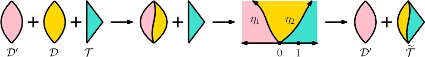
Figure 19: Proposition 6.11 follows from Proposition 6.10 and Theorem 4.2 by conformally welding quantum surfaces in different orders.

As a consequence of Theorem 1.2, we have the following. Recall the notion ${\mathcal{M}}^{\mathrm{disk}}_{2,\bullet}(W)$ for $W>0$ in Section 2.2.

Lemma 6.12.

For some constant depending only on $W$ and $\gamma$, we have ${\mathcal{M}}^{\mathrm{disk}}_{2,\bullet}(W)=C\mathrm{QT}(W,W,2)$.

Proof.

For $W\neq\frac{\gamma^{2}}{2}$, the claim follows from  [AHS20, Proposition 4.4] and [AHS21, Proposition 2.18]. If $W=\frac{\gamma^{2}}{2}$, then consider the conformal welding $(\mathcal{D},\eta)$ of two weight $\frac{\gamma^{2}}{4}$ quantum disks $\mathcal{D}_{1}$ and $\mathcal{D}_{2}$ as in Theorem 4.2. We weight the law of $(\mathcal{D}_{1},\mathcal{D}_{2})$ by the right boundary length of $\mathcal{D}_{2}$ and sample a marked point on the right boundary of $\mathcal{D}_{2}$ according to the quantum length measure. Then it follows from Definition 2.13 that the law of $(\mathcal{D},\eta)$ is some constant times ${\mathcal{M}}^{\mathrm{disk}}_{2,\bullet}(\frac{\gamma^{2}}{2})\otimes\mathrm{SLE}_{\kappa}(\frac{\kappa}{4}-2;\frac{\kappa}{4}-2)$. On the other hand, from the $W\neq\frac{\gamma^{2}}{2}$ case, we can also view $\mathcal{D}_{2}$ as a quantum triangle of weights $\frac{\gamma^{2}}{4},\frac{\gamma^{2}}{4},2$. Then by Theorem 1.1, the law of $(\mathcal{D},\eta)$ is a constant multiple of $\mathrm{QT}(\frac{\gamma^{2}}{2},\frac{\gamma^{2}}{2},2)\otimes\mathrm{SLE}_{\kappa}(\frac{\kappa}{4}-2;\frac{\kappa}{4}-2)$. This concludes the proof. ∎

6.6 Proof of Theorem 1.3

We prove the statement by inductively applying Theorem 1.1. When $n=1$, there is only one marked point with the law of $\eta_{1}$ being $\mathrm{SLE}_{\kappa}(-\frac{\theta_{1}\chi}{\lambda}-1;\frac{\theta_{1}\chi}{\lambda}-1)$, and from Theorem 4.2 we directly see that the weight 2 disk is the welding of a disk of weight $W_{0}=1-\frac{\theta_{1}\chi}{\lambda}$ and a disk of weight $W_{0}=1+\frac{\theta_{1}\chi}{\lambda}$.

Suppose we have proved the statement for the case with $n$ marked boundary points on the real line. Recall that from [AHS21, Definition 2.3] a sample from $\mathrm{QD}_{0,n+1}$ can obtained by first sampling $(\mathbb{H},\phi,\infty)/{\sim_{\gamma}}$ from $\nu_{\phi}(\mathbb{R})^{n}\mathrm{QD}_{0,1}$ and then independently sampling the marked points $w_{1},...,w_{n}$ on $\mathbb{R}$ according to $\nu_{\phi}^{\#}$. We start by claiming that the following two procedures agree:

1. Sample $(\mathbb{H},\phi,w_{1},...,w_{n+1},\infty)/{\sim_{\gamma}}$ from $\mathrm{QD}_{0,n+2}$ and let $z_{1}\leq...\leq z_{n+1}$ be the reordering of $(w_{1},...,w_{n+1})$. Output $(\mathbb{H},\phi,z_{1},...,z_{n+1},\infty)/{\sim_{\gamma}}$.

2. Sample $(\mathbb{H},\phi,\tilde{w}_{1},...,\tilde{w}_{n},\infty)/{\sim_{\gamma}}$ from $(n+1)s_{n+1}\mathrm{QD}_{0,n+1}$ where $\tilde{z}_{1}\leq...\leq\tilde{z}_{n}$ is the reordering of $(\tilde{w}_{1},...,\tilde{w}_{n})$ and $s_{n+1}=\nu_{\phi}((\tilde{z}_{n},\infty))$. Then sample $\tilde{z}_{n+1}$ from $(\nu_{\phi}|_{(\tilde{z}_{n},\infty)})^{\#}$. Output $(\mathbb{H},\phi,\tilde{z}_{1},...,\tilde{z}_{n+1},\infty)/{\sim_{\gamma}}$.

Let $\mathcal{L}$ and $\tilde{\mathcal{L}}$ be the corresponding law of the quantum surfaces. To prove the claim, we start with a sample $(\mathbb{H},\phi,\infty)/\sim_{\gamma}$ from $\mathrm{QD}_{0,1}$ and let $\ell_{i}$ (resp. $\tilde{\ell}_{i}$) be the quantum length of $(-\infty,z_{i})$ (resp. $(-\infty,\tilde{z}_{i})$). Then by our definition, for any non-negative functions $f_{1},...,f_{n+1}$ on $\mathbb{R}$ and $F$ on $H^{-1}(\mathbb{H})$,

$$\mathcal{L}\big{[}F(\phi)f_{1}(\ell_{1})...f_{n+1}(\ell_{n+1})\big{]}=\int\int_{(0,\nu_{\phi}(\mathbb{R}))^{n+1}}(n+1)!\mathbf{1}_{\ell_{1}\leq...\leq\ell_{n+1}}f_{1}(\ell_{1})...f_{n+1}(\ell_{n+1})d\ell_{1}...d\ell_{n+1}\mathrm{QD}_{0,1}(d\phi).$$ (6.21)

On the other hand,

$$\begin{split}\tilde{\mathcal{L}}&\big{[}F(\phi)f_{1}(\tilde{\ell}_{1})...f_{n+1}(\tilde{\ell}_{n+1})\big{]}=\\ &=\int\int_{(0,\nu_{\phi}(\mathbb{R}))^{n}}n!\mathbf{1}_{\tilde{\ell}_{1}\leq...\leq\tilde{\ell}_{n}}f_{1}(\tilde{\ell}_{1})...f_{n}(\tilde{\ell}_{n})\big{(}\int_{\tilde{\ell}_{n}}^{\nu_{\phi}(\mathbb{R})}(n+1)f_{n+1}(\tilde{\ell}_{n+1})d\tilde{\ell}_{n+1}\big{)}d\tilde{\ell}_{1}...d\tilde{\ell}_{n}\mathrm{QD}_{0,1}(d\phi)\\ &=\mathcal{L}\big{[}F(\phi)f_{1}(\ell_{1})...f_{n+1}(\ell_{n+1})\big{]},\end{split}$$ (6.22)

which justifies our claim.

From this claim, we may first sample the left $n$ marked points $z_{1}<...<z_{n}$, which produces a disk $(\mathbb{H},\phi,z_{1},...,z_{n},\infty)/\sim_{\gamma}$ from the measure $\mathrm{QD}_{0,n+1}$ weighted by the right most boundary arc. Then by our induction hypothesis, as we grow the $\theta_{i}$ angle flow lines of the zero boundary GFF, this splits the quantum disk into $n+1$ parts given by

$$\begin{split}\int_{[0,\infty)^{n+1}}s_{n+1}&\mathrm{Weld}\Big{(}{\mathcal{M}}^{\mathrm{disk}}_{2}(W_{0};s_{1}),\mathrm{QT}(W^{1}_{1},W^{2}_{1},W^{3}_{1};s_{1},s_{2}),\\ &\cdots,\mathrm{QT}(W^{n-1}_{1},W^{n-1}_{2},W^{n-1}_{3};s_{n-1},s_{n}),{\mathcal{M}}^{\mathrm{disk}}_{2}(\tilde{W}_{n};s_{n},s_{n+1})\Big{)}ds_{1}\cdots ds_{n+1}.\end{split}$$ (6.23)

where $W_{0}=1-\frac{\theta_{1}\chi}{\lambda}$, $W_{i}^{1}=\frac{(\theta_{i}-\theta_{i+1})\chi}{\lambda}$, $W_{i}^{2}=1+\frac{\theta_{i}\chi}{\lambda}$, $W_{i}^{3}=1-\frac{\theta_{i}\chi}{\lambda}$ for $i=1,...,n-1$ and $\tilde{W}_{n}=1+\frac{\theta_{n}\chi}{\lambda}$. Then from Definition 2.13 and Definition 2.15, as we add the point $z_{n+1}$ onto $(z_{n},\infty)$ according to the quantum length measure, the rightmost surface $D_{n}$ has law ${\mathcal{M}}^{\mathrm{disk}}_{2,\bullet}(\tilde{W}_{n})$, which by Lemma 6.12 is a constant times $\mathrm{QT}(\tilde{W}_{n},\tilde{W}_{n},2)$. Now conditioned on the points $z_{1},...,z_{n}$ and $\eta_{1},...,\eta_{n}$, from [MS16a, Theorem 1.1], the curve $\eta_{n+1}$ has law $\mathrm{SLE}_{\kappa}(-\frac{\theta_{n+1}\chi}{\lambda}-1,-\frac{\theta_{n}\chi}{\lambda}-1;\frac{\theta_{n+1}\chi}{\lambda}-1)$ from $z_{n+1}$ to $\infty$ within the surface $D_{n}$. Therefore by Theorems 1.1 we know $\eta_{n+1}$ cuts $D_{n}$ into a triangle of weight $(W_{n}^{1},W_{n}^{2},W_{n}^{3})=(\frac{(\theta_{n}-\theta_{n+1})\chi}{\lambda},1+\frac{\theta_{n}\chi}{\lambda},1-\frac{\theta_{n}\chi}{\lambda})$ and a disk of weight $W_{n+1}=\frac{\theta_{n+1}\chi}{\lambda}+1$. This finishes the induction step and concludes the proof.

∎

7 Applications to $\mathrm{SLE}$

As an application of our main theorems, in this section we look into several properties of $\mathrm{SLE}_{\kappa}(\rho_{-};\rho_{+},\rho_{1})$ curves. We comment on the relationship between the SLE reversibility and our conformal welding in Section 7.1, compute the moment of the SLE conformal radius in Section 7.2, and finally in Section 7.3 we describe the SLE commutation relation derived from Theorem 1.2.

7.1 Comments on $\mathrm{SLE}_{\kappa}(\rho_{-};\rho_{+},\rho_{1})$ reversibility

In Section 3.3, we proved the $\mathrm{SLE}_{\kappa}(\rho_{-};\rho_{+},\rho_{1})$ reversibility statement in Theorem 1.5 by extending the results in [Zha22] via a conformal map composition argument. It served as a key ingredient in the proof of Theorem 1.2. However, for a certain range of weights we can prove Theorem 1.2 independently of Theorem 1.5, just by reversing the orientation of the curve in (1.5) and applying Proposition 6.3. We record this proof because this is how we originally reached the statement of Theorem 1.5. Moreover, it demonstrates that conformal welding of finite area LQG surfaces is a natural tool for studying the time reversal of SLE curves.

Alternative proof of Theorem 1.2 for $\max\{W_{1},W_{2}\}\geq 2$ and $|W_{1}-W_{2}|<2$.

First assume $\frac{\gamma^{2}}{2}\notin\{W_{1},W_{2},W+W_{1},W+W_{2},W_{3},W_{1}-W_{2}+2\}$. By Proposition 6.8 along with the change weight argument Proposition 6.3, we may assume that $0<W_{1}<W_{2}$, $W_{2}>2$ and $W_{3}=W_{1}-W_{2}+2$. (If $W_{2}=2$ we may apply Lemma 6.7.) Since we know the law of the field by Proposition 6.1, it remains to identify the law of the interface without applying Theorem 1.5. Consider the setting of right panel of Figure 18 where we start with a quantum triangle of weight $(W+W_{1},W+W_{2},W_{3})$ embedded as $(D,\phi,a_{1},a_{2},a_{3})$ and curves $(\eta_{1},\eta_{2})$ such that the surfaces $(S_{1},S_{2},S_{3})$ are independent quantum disks and triangles from

$$\iint_{\mathbb{R}_{+}^{2}}\mathrm{Weld}({\mathcal{M}}^{\mathrm{disk}}_{2}(W;\ell_{1}),\mathrm{QT}(W_{1},W_{2},W_{1}-W_{2}+2;\ell_{1},\ell_{2}),{\mathcal{M}}^{\mathrm{disk}}_{2}(W_{1}-W_{2};\ell_{2}))\ d\ell_{1}\ d\ell_{2}$$

conditioned on having the same interface length as following from Proposition 6.1. Then we know that the marginal law of $\eta_{1}$ is $\mathrm{SLE}_{\kappa}(W-2;W_{2}-2)$, while by Proposition 6.8 (since $W_{1}>W_{1}-W_{2}+2$) the conditional law of $\eta_{2}$ given $\eta_{1}$ is $\mathrm{SLE}_{\kappa}(W_{1}-W_{2},2-W_{2};W_{2}-W_{1}-2)$. Therefore we can read off the conditional law of $\eta_{1}$ given $\eta_{2}$, which is $\mathrm{SLE}_{\kappa}(W-2;W_{2}-2,W_{1}-W_{2})$, and we conclude the proof by reweighting.

Finally if $\frac{\gamma^{2}}{2}\in\{W_{1},W_{2},W+W_{1},W+W_{2},W_{3},W_{1}-W_{2}+2\}$, the result follows from the same limiting argument as in Section 6.5. ∎

From this argument, we immediately obtain the following case of Theorem 1.5.

Proposition 7.1.

Theorem 1.5 holds for $\max\{\rho_{+},\rho_{+}+\rho_{1}\}\geq 0$ and $|\rho_{1}|\leq 2$.

Proof.

The claim follows immediately by reversing the direction of the curve $\eta$ in Theorem 1.2. ∎

7.2 $\mathrm{SLE}_{\kappa}(\rho_{-};\rho_{+},\rho_{1})$ conformal radius

In this section, as an application of Theorem 1.2, we shall prove Theorem 1.4. Since the method is almost identical to that in [AHS21, Section 5], we will be brief and only list the key steps.

Recall that by Theorem 1.2, the weights of the SLE curve are determined by $\rho_{-}=W-2$, $\rho_{+}=W_{2}-2$ and $\rho_{1}=W_{1}-W_{2}$. Define the function $m(\beta_{-},\beta_{1},\beta_{2},\alpha):=\mathbb{E}[\psi_{\eta}^{\prime}(1)^{\alpha}]$, where $\eta$ is an $\mathrm{SLE}_{\kappa}(W_{-}-2;W_{2}-2,W_{1}-W_{2})$ curve and $\psi_{\eta}$ is the mapping-out function defined in Section 1.4. Recall that $\alpha_{0}=\frac{1}{\kappa}(\rho_{+}+2)(\rho_{+}+\rho_{1}+4-\frac{\kappa}{2})=\frac{1}{\kappa}W_{-}(W_{1}+2-\frac{\kappa}{2})$. To start with, we need the following result on weight 2 and weight $\frac{\gamma^{2}}{2}$ quantum disks.

Lemma 7.2 (Propositions 7.7 and 7.8 of [AHS20]).

For $\ell,r>0$, there are constants $C_{1},C_{2}$ such that

$$|{\mathcal{M}}^{\mathrm{disk}}_{2}(2;l,r)|=C_{1}(\ell+r)^{-\frac{4}{\gamma^{2}}-1}\ \ \text{and}\ \ |{\mathcal{M}}^{\mathrm{disk}}_{2}(\frac{\gamma^{2}}{2};l,r)|=C_{2}\frac{(\ell r)^{4/\gamma^{2}-1}}{(\ell^{4/\gamma^{2}}+r^{4/\gamma^{2}})^{2}}.$$ (7.1)

The cases $\beta_{-}\in\{\gamma,Q\}$ correspond to $W_{-}\in\{\frac{\gamma^{2}}{2},2\}$, and for weight $W_{-}$ quantum disks Lemma 7.2 gives the boundary lengths law. Combining with our conformal welding result, we solve for special values of $m$.

Lemma 7.3.

For $\beta_{1},\beta_{2}<Q+\frac{\gamma}{2}$ with $\beta_{1},\beta_{2}\neq Q$, $\alpha<\alpha_{0}$, let $\beta$ be either solution to (1.12). Then we have

$$m(\gamma,\beta_{1},\beta_{2},\alpha)=\frac{\Gamma(\frac{2}{\gamma}(Q-\frac{\beta_{1}+\beta_{2}-\beta}{2}))\Gamma(\frac{2}{\gamma}(2Q-\frac{\beta_{1}+\beta_{2}+\beta}{2}))}{\Gamma(\frac{2}{\gamma}(Q+\frac{2}{\gamma}-\beta_{1}))\Gamma(\frac{2}{\gamma}(Q+\frac{\gamma}{2}-\beta_{2}))},$$ (7.2)

$$m(Q,\beta_{1},\beta_{2},\alpha)=\frac{\Gamma(\frac{\gamma}{2}(Q-\frac{\beta_{1}+\beta_{2}-\beta}{2}))\Gamma(\frac{\gamma}{2}(2Q-\frac{\beta_{1}+\beta_{2}+\beta}{2}))}{\Gamma(\frac{\gamma}{2}(Q+\frac{2}{\gamma}-\beta_{1}))\Gamma(\frac{\gamma}{2}(Q+\frac{\gamma}{2}-\beta_{2}))}.$$ (7.3)

Proof.

Let $\widetilde{\mathrm{QT}}(W_{1},W_{2},\beta_{3})$ be the corresponding quantum surface when the weight $W_{3}$ vertex is replaced by a $\beta_{3}$ Liouville field insertion and the constant $\frac{1}{\gamma(Q-\beta_{1})(Q-\beta_{2})(Q-\beta_{3})}$ is dropped. Then by Proposition 6.3, (1.8) continues to hold with ${\mathrm{QT}}(W_{1},W_{2},W_{3})$ and $\mathrm{QT}(W_{1}+W,W_{2}+W,W_{3})$ replaced by $\widetilde{\mathrm{QT}}(W_{1},W_{2},\beta_{3})$ and $\widetilde{\mathrm{QT}}(W_{1}+W,W_{2}+W,\beta_{3})$ as long as the Seiberg bounds (2.19) holds for $\widetilde{\mathrm{QT}}(W_{1},W_{2},\beta_{3})$. Let $\beta_{3}\in(\max\{|2Q-\beta_{1}-\beta_{2}|,|\beta_{1}-\beta_{2}|\},4Q-\beta_{1}-\beta_{2})$. A sample from the left hand side of (1.8) now has left boundary length law $1_{x>0}\mathfrak{C}x^{\frac{\beta_{1}+\beta_{2}+\beta_{3}-2Q}{\gamma}-\frac{4}{\gamma^{2}}-1}dx$ with $\mathfrak{C}=\frac{2}{\gamma}|\bar{H}_{(0,1,0)}^{(\beta_{1}-\frac{2}{\gamma},\beta_{2}-\frac{2}{\gamma},\beta_{3})}|m(\gamma,\beta_{1},\beta_{2},\alpha_{3})$ where $\alpha_{3}$ is determined by $\beta_{3}$ via (1.12). On the other hand, evaluating this using the right hand side of (1.8), we see that for some constants $c_{\beta_{1},\beta_{2}},\tilde{c}_{\beta_{1},\beta_{2}}$ not depending on $\beta_{3}$,

$$\begin{split}\mathfrak{C}&=\frac{2}{\gamma}c_{\beta_{1},\beta_{2}}\int_{0}^{\infty}|{\mathcal{M}}^{\mathrm{disk}}_{2}(2;1,\ell)|\cdot|\bar{H}_{(0,1,0)}^{(\beta_{1},\beta_{2},\beta_{3})}|\ell^{\frac{\beta_{1}+\beta_{2}+\beta_{3}-2Q}{\gamma}-1}d\ell\\ &=\frac{2}{\gamma}\tilde{c}_{\beta_{1},\beta_{2}}{\Gamma(\frac{\beta_{1}+\beta_{2}+\beta_{3}-2Q}{\gamma})\Gamma(\frac{4}{\gamma^{2}}+1+\frac{2Q-\beta_{1}+\beta_{2}+\beta_{3}}{\gamma})}.\end{split}$$ (7.4)

Using the definition of $\bar{H}_{(0,1,0)}^{(\beta_{1},\beta_{2},\beta_{3})}$ and the shift relations (2.15), this implies that for some constant $C_{\beta_{1},\beta_{2}}$ not depending on $\beta_{3}$ we have

$$m(\gamma,\beta_{1},\beta_{2},\alpha_{3})=C_{\beta_{1},\beta_{2}}\Gamma(\frac{1}{\gamma}(4Q-\beta_{1}-\beta_{2}-\beta_{3}))\Gamma(\frac{1}{\gamma}(2Q-\beta_{1}-\beta_{2}+\beta_{3})).$$ (7.5)

Exactly as in [AHS21, Section A.2], the input [MW17, Theorem 1.8] can be bootstrapped to give $\mathbb{E}[\psi_{\eta}^{\prime}(1)^{\alpha}]<\infty$ for any $\alpha<\alpha_{0}$. By Fubini’s theorem and Morera’s theorem, it is not hard to observe that $\alpha\mapsto\mathbb{E}[\psi_{\eta}^{\prime}(1)^{\alpha}]$ is holomorphic on $\{\alpha\in\mathbb{C}:\textup{Re}\ \alpha<\alpha_{0}\}$. From the uniqueness of holomorphic extensions, we observe that the equation (7.5) extends to any $\alpha<\alpha_{0}$. Therefore by setting $\alpha=0$ (and $\beta_{3}=\beta_{1}-\beta_{2}+\gamma$), we can solve for the constant $C_{\beta_{1},\beta_{2}}$ as $m(\gamma,\beta_{1},\beta_{2},0)$ is trivially 1. Substituting this expression of $C_{\beta_{1},\beta_{2}}$ in (7.5) gives (7.2). By a similar argument one obtains (7.3).

∎

The next step is to establish the shift relations by conformal map composition.

Lemma 7.4.

For $\beta_{-},\tilde{\beta},\beta_{1},\beta_{2}<Q+\frac{\gamma}{2}$ and $\alpha<0$, we have

$$m(\beta_{-}+\tilde{\beta}-Q-\frac{\gamma}{2},\beta_{1},\beta_{2},\alpha)=m(\tilde{\beta},\beta_{1}+\beta_{-}-\gamma-\frac{2}{\gamma},\beta_{2}+\beta_{-}-\gamma-\frac{2}{\gamma},\alpha)m(\beta_{-},\beta_{1},\beta_{2},\alpha).$$ (7.6)

In particular, if $\beta$ solves (1.12), then

$$\frac{m(\beta_{-}-\frac{2}{\gamma},\beta_{1},\beta_{2},\alpha)}{m(\beta_{-},\beta_{1},\beta_{2},\alpha)}=\frac{\Gamma(\frac{2}{\gamma}(2Q+\frac{\gamma-\beta_{1}-\beta_{2}-2\beta_{-}+\beta}{2}))\Gamma(\frac{2}{\gamma}(3Q+\frac{\gamma-\beta_{1}-\beta_{2}-2\beta_{-}-\beta}{2}))}{\Gamma(\frac{2}{\gamma}(3Q-\beta_{1}-\beta_{-}))\Gamma(\frac{2}{\gamma}(2Q+\gamma-\beta_{2}-\beta_{-}))};$$ (7.7)

$$\frac{m(\beta_{-}-\frac{\gamma}{2},\beta_{1},\beta_{2},\alpha)}{m(\beta_{-},\beta_{1},\beta_{2},\alpha)}=\frac{\Gamma(\frac{\gamma}{2}(2Q+\frac{\gamma-\beta_{1}-\beta_{2}-2\beta_{-}+\beta}{2}))\Gamma(\frac{\gamma}{2}(3Q+\frac{\gamma-\beta_{1}-\beta_{2}-2\beta_{-}-\beta}{2}))}{\Gamma(\frac{\gamma}{2}(3Q-\beta_{1}-\beta_{-}))\Gamma(\frac{\gamma}{2}(2Q+\gamma-\beta_{2}-\beta_{-}))}.$$ (7.8)

Proof.

Let $\rho_{-}=\gamma^{2}-\gamma\beta_{-}$, $\rho_{+}=\gamma^{2}-\gamma\beta_{2}$, $\rho_{1}=\gamma(\beta_{2}-\beta_{1})$ and $\tilde{\rho}=\gamma^{2}-\gamma\tilde{\rho}$. Sample an $\mathrm{SLE}_{\kappa}(\tilde{\rho};\rho_{-}+\rho_{+}+2,\rho_{1})$ curve $\eta_{1}$ in $\mathbb{H}$ from 0 to $\infty$, and an $\mathrm{SLE}_{\kappa}({\rho_{-}};\rho_{+},\rho_{1})$ curve $\eta_{2}$ in the connected component of $\mathbb{H}\backslash\eta_{1}$ with $1$ on its boundary. Let $\psi_{{\eta}_{2}|{\eta}_{1}}$ be the conformal map from the right component of $\mathbb{H}\backslash\psi_{{\eta}_{1}}({\eta}_{2})$ to $\mathbb{H}$ fixing $0,1,\infty$. As in the proof of Theorem 1.5, we know $\psi_{\eta_{2}}=\psi_{\eta_{2}|\eta_{1}}\circ\psi_{\eta_{1}}$ and $\psi_{\eta_{2}|\eta_{1}}$ and $\psi_{\eta_{1}}$ are independent. Moreover, using the imaginary geometry, the marginal law of $\eta_{2}$ is $\mathrm{SLE}_{\kappa}({\rho_{-}+\tilde{\rho}+2};\rho_{+},\rho_{1})$. Therefore (7.6) follows from $\mathbb{E}[\psi_{\eta_{2}}^{\prime}(1)^{\alpha}]=\mathbb{E}[\psi_{\eta_{2}|\eta_{1}}^{\prime}(1)^{\alpha}]\mathbb{E}[\psi_{\eta_{1}}^{\prime}(1)^{\alpha}]$. Equations (7.7) and (7.8) follow by setting $\tilde{\beta}\in\{\gamma,Q\}$ and applying Lemma 7.3. ∎

Set $g(\beta_{-},\beta_{1},\beta_{2},\alpha)$ to be the right hand side of (1.13), that is

$$g(\beta_{-},\beta_{1},\beta_{2},\alpha)=\frac{F(\beta+\beta_{2}-\beta_{1},\gamma^{2},\gamma^{2}-\gamma\beta_{-},\gamma^{2}-\gamma\beta_{2},\gamma(\beta_{2}-\beta_{1}))}{F(\gamma,\gamma^{2},\gamma^{2}-\gamma\beta_{-},\gamma^{2}-\gamma\beta_{2},\gamma(\beta_{2}-\beta_{1}))}.$$

Define $h(\beta_{-},\beta_{1},\beta_{2},\alpha):=\frac{m(\beta_{-},\beta_{1},\beta_{2},\alpha)}{g(\beta_{-},\beta_{1},\beta_{2},\alpha)}$. Using the argument in [AHS21, Section A.3], it is not hard to show that $h$ is meromorphic on $\{\alpha:\textup{Re}\ \alpha<0\}$. By the shift relations (2.15), we see

$$\begin{split}&h(\beta_{-}-\frac{2}{\gamma},\beta_{1},\beta_{2},\alpha)=h(\beta_{-},\beta_{1},\beta_{2},\alpha)\ \text{for}\ \beta_{-},\beta_{1},\beta_{2}<Q+\frac{\gamma}{2};\\ &h(\beta_{-}-\frac{\gamma}{2},\beta_{1},\beta_{2},\alpha)=h(\beta_{-},\beta_{1},\beta_{2},\alpha)\ \text{for}\ \beta_{-},\beta_{1},\beta_{2}<Q+\frac{\gamma}{2}.\end{split}$$ (7.9)

Proof of Theorem 1.4.

We start with the case where $\alpha<0$. First suppose $\gamma^{2}\notin\mathbb{Q}$. Assume $\beta_{1},\beta_{2}\neq Q$. The function $\beta_{-}\mapsto h(\beta_{-},\beta_{1},\beta_{2},\alpha)$ is well-defined on $(-\infty,Q+\frac{\gamma}{2})$ and is constant on a dense subset of $(-\infty,Q+\frac{\gamma}{2})$ by (7.9). Moreover, by Lemma 7.3 we know that $h(\gamma,\beta_{1},\beta_{2},\alpha)=1$ and therefore $m(\beta_{-},\beta_{1},\beta_{2},\alpha)=g(\beta_{-},\beta_{1},\beta_{2},\alpha)$ on a dense subset of $(-\infty,Q+\frac{\gamma}{2})$. On the other hand, since $\psi_{\eta}^{\prime}(1)>1$, a.s., it follows that $m(\beta_{-},\beta_{1},\beta_{2},\alpha)<1$ whenever $\alpha<0$, and therefore by (7.6) the function $\beta_{-}\mapsto m(\beta_{-},\beta_{1},\beta_{2},\alpha)$ is monotone. This proves (1.13) for $\beta_{1},\beta_{2}\neq Q$, and for $Q\in\{\beta_{1},\beta_{2}\}$, the claim follows by applying (7.6) to $(Q+\frac{\gamma}{2}-\varepsilon,\beta_{-},\beta_{1}+\varepsilon,\beta_{2}+\varepsilon)$ for $\varepsilon>0$ chosen to be small.

Now assume $\gamma^{2}\in\mathbb{Q}$. By the same SLE continuity argument as in [AHS21, Lemma A.3], for $\eta_{n}\sim\mathrm{SLE}_{\kappa_{n}}(\rho_{-};\rho_{+},\rho_{1})$ and $\eta\sim\mathrm{SLE}_{\kappa}(\rho_{-};\rho_{+},\rho_{1})$ with $\kappa_{n}\downarrow\kappa\in(0,4)$, when $\rho_{-},\rho_{+},\rho_{+}+\rho_{1}\geq\frac{\kappa}{2}-2$, i.e., the curves are non-boundary hitting, $\psi_{\eta_{n}}^{\prime}(1)\to\psi_{\eta}^{\prime}(1)$ in probability. This implies $m(\beta_{-},\beta_{1},\beta_{2},\alpha)=g(\beta_{-},\beta_{1},\beta_{2},\alpha)$ for $\beta_{-},\beta_{1},\beta_{2}\leq Q$ and all $\kappa\in(0,4)$. Then for $\beta_{-}\leq\frac{2}{\gamma}$, $\beta_{1},\beta_{2}<Q+\frac{\gamma}{2}$, $m(\beta_{-},\beta_{1},\beta_{2},\alpha)$ is solved by applying (7.6) along with (7.3) for the tuple $(Q,\beta_{-}+\frac{\gamma}{2},\beta_{1},\beta_{2})$, and the general $\beta_{-},\beta_{1},\beta_{2}<Q+\frac{\gamma}{2}$ case follows immediately by applying (7.6) to the tuple $(\beta_{-},\frac{2}{\gamma},\beta_{1},\beta_{2})$.

Finally, again by using the holomorphic extension in terms of $\alpha$, (1.13) extends to the full range $\alpha<\alpha_{0}$, as desired. ∎

7.3 SLE commutation relation

In Imaginary geometry theory, the GFF flow line construction neatly characterizes the marginal and conditional laws of interacting $\mathrm{SLE}_{\kappa}(\underline{\rho})$ curves. On the other hand, we can also read off the interface laws in the conformal welding statement in Theorem 1.2. By considering the different orders of welding quantum disks and triangles, this gives an alternative way of describing the marginal and conditional laws of $\mathrm{SLE}_{\kappa}(\rho_{-};\rho_{+},\rho_{1})$ curves. Moreover, this also extends to $\widetilde{\mathrm{SLE}}_{\kappa}(\rho_{-};\rho_{+},\rho_{1};\alpha)$, the $\mathrm{SLE}$ curves weighted by conformal radius.

As a quick application, we prove the following.

Proposition 7.5.

Fix $W,W^{\prime},W_{1},W_{2},W_{3}>0$. The following two laws on tuples of curves $(\eta_{1},\eta_{2})$ differs only by a multiplicative constant. Let $\alpha$ be the same as (1.7) and

$$\alpha^{\prime}=\frac{W_{2}+W_{3}-W_{1}-2}{4\kappa}({W_{2}+W_{1}+2-W_{3}-\kappa}).$$

1. First sample an $\widetilde{\mathrm{SLE}}_{\kappa}(W-2;W_{2}-2,W_{1}-W_{2}+W^{\prime};\alpha)$ (with force points $0^{-},0^{+},1$) curve $\eta_{1}$ on $\mathbb{H}$ from 0 to $\infty$, and then sample an $\widetilde{\mathrm{SLE}}_{\kappa}(W_{3}-2,W_{1}-W_{3};W^{\prime}-2;\alpha^{\prime})$ (with force points $1^{-},0,1^{+}$) curve $\eta_{2}$ to the right of $\eta_{1}$ in $\mathbb{H}\backslash\eta_{1}$.

2. First sample an $\widetilde{\mathrm{SLE}}_{\kappa}(W_{3}-2,W_{1}-W_{3}+W;W^{\prime}-2;\alpha^{\prime})$ (with force points $1^{-},0,1^{+}$) curve $\eta_{2}$ on $\mathbb{H}$ from 1 to $\infty$, and then sample an $\widetilde{\mathrm{SLE}}_{\kappa}(W-2;W_{2}-2,W_{1}-W_{2};\alpha)$ (with force points $0^{-},0^{+},1$) curve $\eta_{1}$ on the left component of $\mathbb{H}\backslash\eta_{2}$.

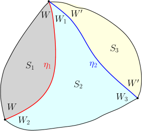
Figure 20: Proof of Proposition 7.5. If we start by welding $S_{1}$ to the left of $S_{2}$ first and then $S_{3}$ to the right, then by Theorem 1.2 we know the marginal law of $\eta_{2}$ and the law of $\eta_{1}$ given $\eta_{2}$. If we first weld $S_{3}$ to the right of $S_{2}$ and $S_{1}$ to the left, then we can interpret the marginal law of $\eta_{1}$ and then the conditional law of $\eta_{2}$ given $\eta_{1}$. This justifies Proposition 7.5.

Proof.

The proof is again an application of Theorem 1.2 and the argument in Section 6.3. Namely, suppose we are in the setting of Figure 20, where we sample surfaces $(S_{1},S_{2},S_{3})$ from the measure

$$\iint_{\mathbb{R}_{+}^{2}}\mathrm{Weld}({\mathcal{M}}^{\mathrm{disk}}_{2}(W;\ell_{1}),\mathrm{QT}(W_{1},W_{2},W_{3};\ell_{1},\ell_{2}),{\mathcal{M}}^{\mathrm{disk}}_{2}(W^{\prime};\ell_{2}))\ d\ell_{1}\ d\ell_{2}$$

and conformally weld them together. First consider the case where $W+W^{\prime}+W_{1},W+W_{2},W^{\prime}+W_{3}\geq\frac{\gamma^{2}}{2}$. We may first weld $S_{1}$ and $S_{2}$ together, which implies that given $\eta_{2}$, the conditional law of $\eta_{1}$ is $\widetilde{\mathrm{SLE}}_{\kappa}(W-2;W_{2}-2,W_{1}-W_{2};\alpha)$. Then as we weld $S_{3}$ to the right, we observe that the marginal law of $\eta_{2}$ is proportional to $\widetilde{\mathrm{SLE}}_{\kappa}(W_{3}-2,W_{1}-W_{3}+W;W^{\prime}-2;\alpha^{\prime})$. This implies the interface law $(\eta_{1},\eta_{2})$ is a constant multiple of the second law. On the other hand, if we first fix $S_{1}$ and weld $S_{3}$ to the right of $S_{2}$, and then weld $S_{1}$ to the left, by Theorem 1.2, we know that the conditional law of $\eta_{2}$ given $\eta_{1}$ is a constant times $\widetilde{\mathrm{SLE}}_{\kappa}(W_{3}-2,W_{1}-W_{3};W^{\prime}-2;\alpha^{\prime})$ and the marginal law of $\eta_{1}$ is $\widetilde{\mathrm{SLE}}_{\kappa}(W-2;W_{2}-2,W_{1}-W_{2}+W^{\prime};\alpha)$. If any of the vertex in the large triangle is thin, then we may focus on the thick triangle component. This concludes the proof. ∎

References

- [AHS20] M. Ang, N. Holden, and X. Sun. Conformal welding of quantum disks. arXiv preprint arXiv:2009.08389, 2020.
- [AHS21] Morris Ang, Nina Holden, and Xin Sun. Integrability of SLE via conformal welding of random surfaces. arXiv preprint arXiv:2104.09477, 2021.
- [ARS21] Morris Ang, Guillaume Remy, and Xin Sun. FZZ formula of boundary Liouville CFT via conformal welding. arXiv preprint arXiv:2104.09478, 2021.
- [ARSZ22] Morris Ang, Guillaume Remy, Xin Sun, and Tunan Zhu. Proof of the ponsot-teschner formula for boundary liouville cft. arXiv preprint, 2022.
- [AS21] Morris Ang and Xin Sun. Integrability of the conformal loop ensemble. arXiv preprint arXiv:2107.01788, 2021.
- [AY] Morris Ang and Pu Yu. Radial conformal welding and mating-of-trees in liouville theory. in preparation.
- [Ber17] Nathanaël Berestycki. An elementary approach to gaussian multiplicative chaos. Electronic communications in Probability, 22:1–12, 2017.
- [BGS22] Jacopo Borga, Ewain Gwynne, and Xin Sun. Permutons, meanders, and SLE-decorated Liouville quantum gravity. arXiv e-prints, page arXiv:2207.02319, July 2022.
- [BHSY22] Jacopo Borga, Nina Holden, Xin Sun, and Pu Yu. Baxter permuton and liouville quantum gravity. arXiv preprint arXiv:2203.12176, 2022.
- [BM17] Jérémie Bettinelli and Grégory Miermont. Compact Brownian surfaces I: Brownian disks. Probab. Theory Related Fields, 167(3-4):555–614, 2017.
- [BM22] Jacopo Borga and Mickaël Maazoun. Scaling and local limits of Baxter permutations and bipolar orientations through coalescent-walk processes. Ann. Probab., 50(4):1359–1417, 2022.
- [Bor21] Jacopo Borga. The skew Brownian permuton: a new universality class for random constrained permutations. arXiv e-prints, page arXiv:2112.00156, November 2021.
- [BP21] Nathanaël Berestycki and Ellen Powell. Gaussian free field, liouville quantum gravity and gaussian multiplicative chaos. Lecture notes, 2021.
- [DDDF20] Jian Ding, Julien Dubédat, Alexander Dunlap, and Hugo Falconet. Tightness of Liouville first passage percolation for . Publications mathématiques de l’IHÉS, 132(1):353–403, 2020.
- [DKRV17] François David, Antti Kupiainen, Rémi Rhodes, and Vincent Vargas. Renormalizability of Liouville quantum field theory at the Seiberg bound. Electronic Journal of Probability, 22:1–26, 2017.
- [DMS21] Bertrand Duplantier, Jason Miller, and Scott Sheffield. Liouville quantum gravity as a mating of trees. Astérisque, 427, 2021.
- [DS11] Bertrand Duplantier and Scott Sheffield. Liouville quantum gravity and KPZ. Inventiones mathematicae, 185(2):333–393, 2011.
- [Dub05] Julien Dubédat. SLE (, ) martingales and duality. The Annals of Probability, 33(1):223–243, 2005.
- [Dub07] Julien Dubédat. Commutation relations for schramm-loewner evolutions. Communications on Pure and Applied Mathematics: A Journal Issued by the Courant Institute of Mathematical Sciences, 60(12):1792–1847, 2007.
- [GHS19] Ewain Gwynne, Nina Holden, and Xin Sun. Mating of trees for random planar maps and liouville quantum gravity: a survey. arXiv preprint arXiv:1910.04713, 2019.
- [GM19] Ewain Gwynne and Jason Miller. Convergence of the free Boltzmann quadrangulation with simple boundary to the Brownian disk. Ann. Inst. Henri Poincaré Probab. Stat., 55(1):551–589, 2019.
- [GM21] Ewain Gwynne and Jason Miller. Existence and uniqueness of the Liouville quantum gravity metric for . Invent. Math., 223(1):213–333, 2021.
- [HRV18] Yichao Huang, Rémi Rhodes, and Vincent Vargas. Liouville quantum gravity on the unit disk. Ann. Inst. Henri Poincaré Probab. Stat., 54(3):1694–1730, 2018.
- [Law08] Gregory F Lawler. Conformally invariant processes in the plane. Number 114. American Mathematical Soc., 2008.
- [LSW03] Gregory Lawler, Oded Schramm, and Wendelin Werner. Conformal restriction: the chordal case. Journal of the American Mathematical Society, 16(4):917–955, 2003.
- [MS16a] J. Miller and S. Sheffield. Imaginary Geometry I: Interacting SLEs. Probability Theory and Related Fields, 164(3-4):553–705, 2016.
- [MS16b] Jason Miller and Scott Sheffield. Imaginary geometry II: Reversibility of SLE for . The Annals of Probability, 44(3):1647–1722, 2016.
- [MS17] Jason Miller and Scott Sheffield. Imaginary geometry IV: interior rays, whole-plane reversibility, and space-filling trees. Probab. Theory Related Fields, 169(3-4):729–869, 2017.
- [MS20] Jason Miller and Scott Sheffield. Liouville quantum gravity and the Brownian map I: the metric. Invent. Math., 219(1):75–152, 2020.
- [MS21] Jason Miller and Scott Sheffield. Liouville quantum gravity and the Brownian map II: Geodesics and continuity of the embedding. Ann. Probab., 49(6):2732–2829, 2021.
- [MT09] Sean Meyn and Richard L. Tweedie. Markov chains and stochastic stability. Cambridge University Press, Cambridge, second edition, 2009. With a prologue by Peter W. Glynn.
- [MW17] Jason Miller and Hao Wu. Intersections of sle paths: the double and cut point dimension of sle. Probability Theory and Related Fields, 167(1-2):45–105, 2017.
- [PT02] B. Ponsot and J. Teschner. Boundary Liouville field theory: Boundary three point function. Nucl. Phys. B, 622:309–327, 2002.
- [RV10] Raoul Robert and Vincent Vargas. Gaussian multiplicative chaos revisited. The Annals of Probability, 38(2):605–631, 2010.
- [RZ20] Guillaume Remy and Tunan Zhu. The distribution of Gaussian multiplicative chaos on the unit interval. The Annals of Probability, 48(2):872–915, 2020.
- [RZ22] Guillaume Remy and Tunan Zhu. Integrability of Boundary Liouville Conformal Field Theory. Comm. Math. Phys., 395(1):179–268, 2022.
- [Sch00] Oded Schramm. Scaling limits of loop-erased random walks and uniform spanning trees. Israel Journal of Mathematics, 118(1):221–288, 2000.
- [She16] Scott Sheffield. Conformal weldings of random surfaces: SLE and the quantum gravity zipper. The Annals of Probability, 44(5):3474–3545, 2016.
- [SS13] O. Schrmm and S. Sheffield. A contour line of the continuum Gaussian free field. Probab. Theory Related Fields, 157, 2013.
- [SW16] Scott Sheffield and Menglu Wang. Field-measure correspondence in Liouville quantum gravity almost surely commutes with all conformal maps simultaneously. arXiv preprint arXiv:1605.06171, 2016.
- [Wil74] David Williams. Path decomposition and continuity of local time for one-dimensional diffusions, I. Proceedings of the London Mathematical Society, 3(4):738–768, 1974.
- [Yu22] Pu Yu. Time-reversal of multiple-force-point chordal . arXiv preprint, 2022.
- [Zha08] Dapeng Zhan. Duality of chordal sle. Inventiones mathematicae, 174(2):309, 2008.
- [Zha22] Dapeng Zhan. Time-reversal of multiple-force-point with all force points lying on the same side. Ann. Inst. Henri Poincaré Probab. Stat., 58(1):489–523, 2022.