High-resolution resonant portraits of a single-planet white dwarf system

Abstract

The dynamical excitation of asteroids due to mean motion resonant interactions with planets is enhanced when their parent star leaves the main sequence. However, numerical investigation of resonant outcomes within post-main-sequence simulations is computationally expensive, limiting the extent to which detailed resonant analyses have been performed. Here, we combine the use of a high-performance computer cluster and the general semianalytical libration width formulation of Gallardo et al. (2021) in order to quantify resonant stability, strength and variation instigated by stellar evolution for a single-planet system containing asteroids on both crossing and non-crossing orbits. We find that resonant instability can be accurately bound with only main-sequence values by computing a maximum libration width as a function of asteroid longitude of pericentre. We also quantify the relative efficiency of mean motion resonances of different orders to stabilize versus destabilize asteroid orbits during both the giant branch and white dwarf phases. The $4$:$1$, $3$:$1$ and $2$:$1$ resonances represent efficient polluters of white dwarfs, and even when in the orbit-crossing regime, both the $4$:$3$ and $3$:$2$ resonances can retain small reservoirs of asteroids in stable orbits throughout giant branch and white dwarf evolution. This investigation represents a preliminary step in characterising how simplified extrasolar Kirkwood gap structures evolve beyond the main-sequence.

1 Introduction

The dynamics of post-main-sequence planetary systems are rich. After remaining relatively static for potentially billions of years along the main-sequence, planetary and small body architectures and reservoirs experience significant physical and orbital changes while and after their parent star convulses during its death throes (Veras, 2016).

The end result of many of these changes are manifest in the growing body of observations of planetary remnants close to and within the photospheres of white dwarfs. In fact, dedicated surveys suggest that over a quarter of all Milky Way white dwarfs are currently accreting planetary material (Zuckerman et al., 2003, 2010; Koester et al., 2014), with compositions that vary from rocky, terrestrial-like (Jura & Young, 2014; Doyle et al., 2019) to volatile-rich (Xu et al., 2017) and potentially consistent with primitive planetesimals (Xu et al., 2013; Curry et al., 2022), asteroids or meteorites (Gänsicke et al., 2012; Wilson et al., 2015; Melis & Dufour, 2017; Swan et al., 2019; Buchan et al., 2022), comets (Farihi et al., 2013; Raddi et al., 2015; Hoskin et al., 2020) or moons (Doyle et al., 2021; Klein et al., 2021).

The accretion of planetary matter onto white dwarfs – a process which is commonly known as “white dwarf pollution” – has been observed directly (Cunningham et al., 2022) and is thought to almost always (Rocchetto et al., 2015; Bonsor et al., 2017) originate from Solar radii-scale circumstellar discs. These discs probably represent the debris of broken-up minor planets, and over 60 of these discs have now been observed (e.g. Farihi, 2016; Manser et al., 2020). Their formation has been described dynamically (Jura, 2003; Debes et al., 2012; Veras et al., 2014a; Malamud & Perets, 2020b; Veras & Kurosawa, 2020; Li et al., 2021; Brouwers et al., 2022), and the nature of their progenitor bodies reflects the chemical composition seen in the photospheres of their parent white dwarfs.

This variation in composition and potential progenitor planetary bodies suggests that the dynamical mechanisms which so readily transport planetary material to the close vicinity of white dwarfs are system-specific. Nevertheless, a mechanism which is thought to be common is a sequence of gravitational perturbations generated by a surviving planet and imposed upon a minor body that creates a pathway for the latter to reach the Roche radius of (disruption distance from) the white dwarf.

Mounting investigations of these pathways reveal that they are more likely to be traversed with a greater number of perturbers in the system, whether these be additional planets (Veras et al., 2016; Maldonado et al., 2021; O’Connor et al., 2022) or additional stellar companions (Bonsor & Veras, 2015; Hamers & Portegies Zwart, 2016; Petrovich & Muñoz, 2017; Stephan et al., 2017; Veras et al., 2017). However, in a significant fraction of systems, only one planet may survive. In fact, all known planets orbiting white dwarfs are in single-planet systems (Thorsett et al., 1993; Sigurdsson et al., 2003; Luhman et al., 2011; Gänsicke et al., 2019; Vanderburg et al., 2020; Gaia Collaboration et al., 2022), including the notable case of a roughly Jovian analogue with respect to both planet-star separation and mass (Blackman et al., 2021).

In single-planet, single-star systems, the dynamical pathways for an asteroid or comet to reach the white dwarf are restricted. In the absence of external forces, a planet must be on an eccentric orbit in order to perturb an asteroid into a white dwarf (Antoniadou & Veras, 2016). The external force provided by the star as it traverses the giant branch phases and loses mass can change stability boundaries (Debes & Sigurdsson, 2002; Veras et al., 2013a; Mustill et al., 2014; Veras & Gänsicke, 2015) and thereby allow minor bodies to reach the star (Bonsor et al., 2011; Frewen & Hansen, 2014; Veras et al., 2021), but not always (Veras et al., 2020).

One way to increase a minor body’s eccentricity to a sufficiently high value to reach the white dwarf’s Roche radius is for the minor body to be trapped in a mean-motion resonance with the planet. Although resonances often appear in the post-main-sequence planetary literature, only a few such investigations have actually focussed on the dynamics of resonance. Voyatzis et al. (2013) semi-analytically modelled how stellar mass loss changes the resonant equations of motion, and used the the maximal Lyapunov characteristic number as a chaos indicator to explore relevant regions of phase space. Smallwood et al. (2018, 2021) focussed on the efficiency of secular resonances induced in multi-planet systems after one planet was engulfed. Other studies (Debes et al., 2012; Caiazzo & Heyl, 2017; Veras et al., 2018; Antoniadou & Veras, 2019; Ronco et al., 2020; Veras et al., 2021; Veras & Hinckley, 2021; Li et al., 2022) have included helpful individual plots that demonstrate the reach of particular mean-motion resonances in post-main-sequence planetary systems.

In this paper, we provide a focussed and detailed numerical analysis of post-main-sequence mean-motion resonances in two similar one-planet systems, each containing $10^{5}$ asteroids and differing only in planetary mass. For perspective, this number of asteroids is an order-of-magnitude greater than the number of asteroids we used in the simulations of Veras et al. (2021), and all of the simulations here combine stellar and planetary evolution self-consistently by using the slow but accurate code from Mustill et al. (2018). Here, we combine this computationally expensive suite of numerical integrations of these asteroids with an analysis enabled by employing the general semianalytical resonant characterization code of Gallardo et al. (2021).

A simplified version of this characterization code has been used in a suite of previous papers (Gallardo, 2006, 2019, 2020) and is particularly valuable because it is neither restricted to a particular resonant order nor subject to convergence failures of some disturbing function expansions. The code instead numerically calculates the disturbing function given a complete set of orbital elements and masses, and generates several useful outputs, the most relevant of which for this study is libration width. Such facility is enabled by assuming that the longitudes of pericentre and longitudes of ascending node of both planet and asteroid are fixed throughout the resonant motion (but remain selectable as initial conditions).

Our goals here are four-fold: (i) to provide a detailed resonant map for an evolved planetary architecture covering a wide range of resonant orders, (ii) to determine an efficient way to characterize these resonances, (iii) to determine which resonances can be efficient at perturbing asteroids towards the white dwarf, for this given architecture, and (iv) to determine which resonances can be efficient at ejecting asteroids from the system. This last point is particularly relevant to assess the likely origins of small interstellar free-floaters (Moro-Martín, 2022), of which we might see an increasing number passing through the solar system with the Vera C. Rubin Observatory.

This paper is organized as follows. In Section 2, we describe our simulation setup. We analyze these results in Section 3, and then summarise in Section 4.

2 Simulation setup

Because our objective is to analyze resonant outcomes and constraints for a single-planet system in detail, we carefully chose our simulation initial conditions such that they would generate substantial statistics while still remaining physical and plausible. We were guided by the following considerations:

1. Both asteroids and the planet are subject to destruction from the parent star as it transitions from a main-sequence to a giant branch star. The increase in the star’s size can tidally drag inward and engulf objects out to distances of several au (Kunitomo et al., 2011; Mustill & Villaver, 2012; Nordhaus & Spiegel, 2013; Villaver et al., 2014; Madappatt et al., 2016; Ronco et al., 2020), and the increase in the star’s luminosity could break up asteroids out to tens of au (Veras et al., 2014b; Veras & Scheeres, 2020) and drag debris both inwards and outwards (Veras et al., 2015a, 2019; Ferich et al., 2022). Hence, there is a minimum surviving distance for both the planet and asteroids, and asteroids could occupy a wide swathe of distance space.

2. When the planet mass is too small, the parameter space widths of mean motion resonances with asteroids fail to exceed the resolution achieved in numerical simulations. In other words, in this case, too many asteroids would need to be sampled to clearly detect the resonant signature. On distance scales of au, this critical mass is comparable to that of a Super-Earth or mini-Neptune (Veras et al., 2021). In general then, at the present time, only giant planets produce sufficiently high-resolution signatures in simulations of evolved planetary systems on au-scales for our purposes.

3. Within the solar system, we see resonances between objects which are both on osculating crossing orbits (e.g. Neptune and Pluto) and osculating non-crossing orbits (e.g. some Hecuba gap asteroids). We also detect much higher order resonant signatures (e.g. Fig. 20 of Dermott et al., 2021) than is currently achievable in observations of extrasolar planetary systems, although such signatures undoubtedly exist. Hence, the more types of mean-motion resonances we can sample, the better that we can reflect reality.

4. A planet on a circular orbit very rarely, if ever, can perturb an asteroid close to its parent star (Antoniadou & Veras, 2016; Veras et al., 2021). Hence, a planet on an eccentric orbit would need to be adopted in order to sample white dwarf pollution. Further, planets in evolved planetary systems which would survive to the white dwarf phase are rarely on exactly circular orbits (Grunblatt et al., 2018, 2022), and can only be circularized through subsequent gravitational perturbations and tidal effects by other larger bodies in the same system (Veras & Fuller, 2019, 2020; Muñoz & Petrovich, 2020; O’Connor & Lai, 2020; Stephan et al., 2021) or migration within common envelopes (Chamandy et al., 2021; Lagos et al., 2021; Szölgyén et al., 2022; Yarza et al., 2022).

These considerations have led us to choose a planetary architecture similar to one used in Veras et al. (2021), where, at the end of the main sequence, the planet’s semimajor axis is $a_{\rm pl}=10.5$ au and its eccentricity is $e_{\rm pl}=0.2$. Asteroids are interior to the planet and fill the $(a_{\rm ast},e_{\rm ast})$ parameter space at high resolution, subject to the restriction that their orbital pericentres exceed 2 au and $a_{\rm ast}=4-9$ au.

These choices allowed us to sample a variety of mean-motion commensurabilities: three of first-order ($2$:$1$, $3$:$2$, $4$:$3$), four of second-order ($3$:$1$, $5$:$3$, $7$:$5$, $9$:$7$), four of third-order ($4$:$1$, $5$:$2$, $7$:$4$, $8$:$5$), and numerous ones of slightly higher orders. Our choices also allowed us to sample crossing and non-crossing orbits.

The specifics of our simulation setup are as follows. We treated the asteroids as test particles. Hence, the planet’s orbit was not affected by the asteroids, and we patched together many serial simulations to create a single high-resolution resonant portrait. We did so in order to create two composite simulations, each containing a total of $10^{5}$ test particles. In one composite, the planet’s mass was a Saturn mass, and in the other, the planet’s mass was a Jupiter mass.

For the other orbital elements of the objects, we set the planet’s inclination $i_{\rm pl}$, argument of pericentre $\omega_{\rm pl}$ and longitude of ascending node $\Omega_{\rm pl}$ all to $0^{\circ}$. During stellar evolution, as the star loses mass, both $i_{\rm pl}$ and $\Omega_{\rm pl}$ remain fixed, but $\omega_{\rm pl}$ does vary (Omarov, 1962; Hadjidemetriou, 1963; Veras et al., 2011), assuming isotropic mass loss (Veras et al., 2013b; Dosopoulou & Kalogera, 2016a, b). For the asteroids, we randomly sampled them from uniform distributions of $a_{\rm ast}=3-9$ au and $e_{\rm ast}$, subject to their orbital pericentre $q_{\rm ast}\geq 2$ au. We randomly sampled $i_{\rm ast}$ values from uniform distributions from $0^{\circ}$ to $5^{\circ}$, and randomly chose $\omega_{\rm ast}$ and $\Omega_{\rm ast}$ from uniform distributions from $0^{\circ}$ to $360^{\circ}$.

The host star began as a $M_{\star}^{\rm MS}=2.0M_{\odot}$ main-sequence star and evolved into a $M_{\star}^{\rm WD}=0.637M_{\odot}$ white dwarf, according to the prescription given by SSE code (Hurley et al., 2000). This evolutionary sequence was incorporated within a numerical integration code that propagates planetary orbits. The details of this code are described in Mustill et al. (2018). Here, we used its RADAU integrator, and adopted a tolerance of $10^{-12}$. We started the simulations at the end of the main-sequence phase and ran the system for 10 Myr to clear out a minimum number of asteroids which would not have survived the main-sequence. The simulations then continued through the giant branch phases, and then for 1 Gyr during the white dwarf phase. In total, the simulation duration corresponds to 1.343 Gyr.

We henceforth use the word “instability” to describe a simulation where the asteroid has escaped the system, collided with the planet, or collided with the star. These outcomes contain quantitative subtleties: the boundaries of the system here are assumed to be aspherical according to the Galactic tide, and are changing with mass loss from the evolving star (Veras & Evans, 2013; Veras et al., 2014c). These boundaries form a triaxial ellipsoid, one with semi-axes on the order of $10^{5}$ au, by assuming a Galactocentric distance of 8 kpc. Collisions with the central star were computed by assuming that after the star becomes a white dwarf, its Roche sphere is $1R_{\odot}$: within the code, we hence artificially inflated the star’s radius to this typical value.

3 Simulation results

Although many aspects of the simulation outcomes may be analyzed, in this investigation we focus solely on the resonant-based outputs. A description of other properties and results, with similar but much lower resolution simulations, can be found in Veras et al. (2021). We start here by presenting the full instability portraits (Section 3.1), and then zoom into three different locations: the regime of non-crossing orbits (Section 3.2), the $2$:$1$ resonance (Section 3.3) and the other first-order resonances (Section 3.4). Then, we compare libration widths computed with different sets of initial conditions in Section 3.5, and quantify different resonant strengths and instability outcomes in Section 3.6.

3.1 Full profiles

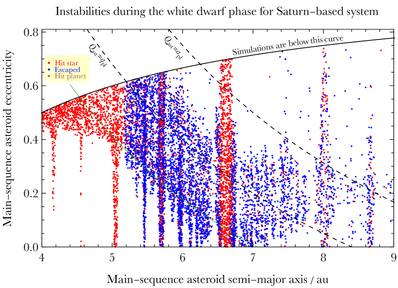
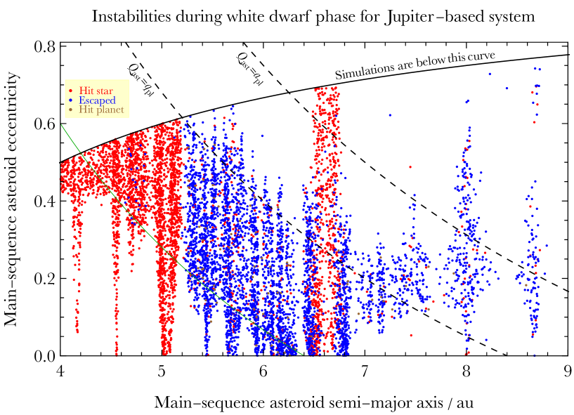
Figure 1: Full resonant instability portraits during the white dwarf phase only, for the Saturn-based architecture (top) and the Jupiter-based architecture (bottom). The planet’s main-sequence semi-major axis is 10.5 au and its eccentricity is 0.2. The black dashed curves indicate where the initial apocentre of the asteroid orbit intersects the initial semimajor axis and pericentre of the planet’s orbit. The solid green curves (starting below the legends) from equation (1) trace out purely analytic close encounter bounds between the planet and asteroids.

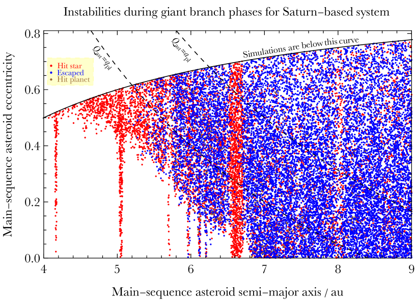
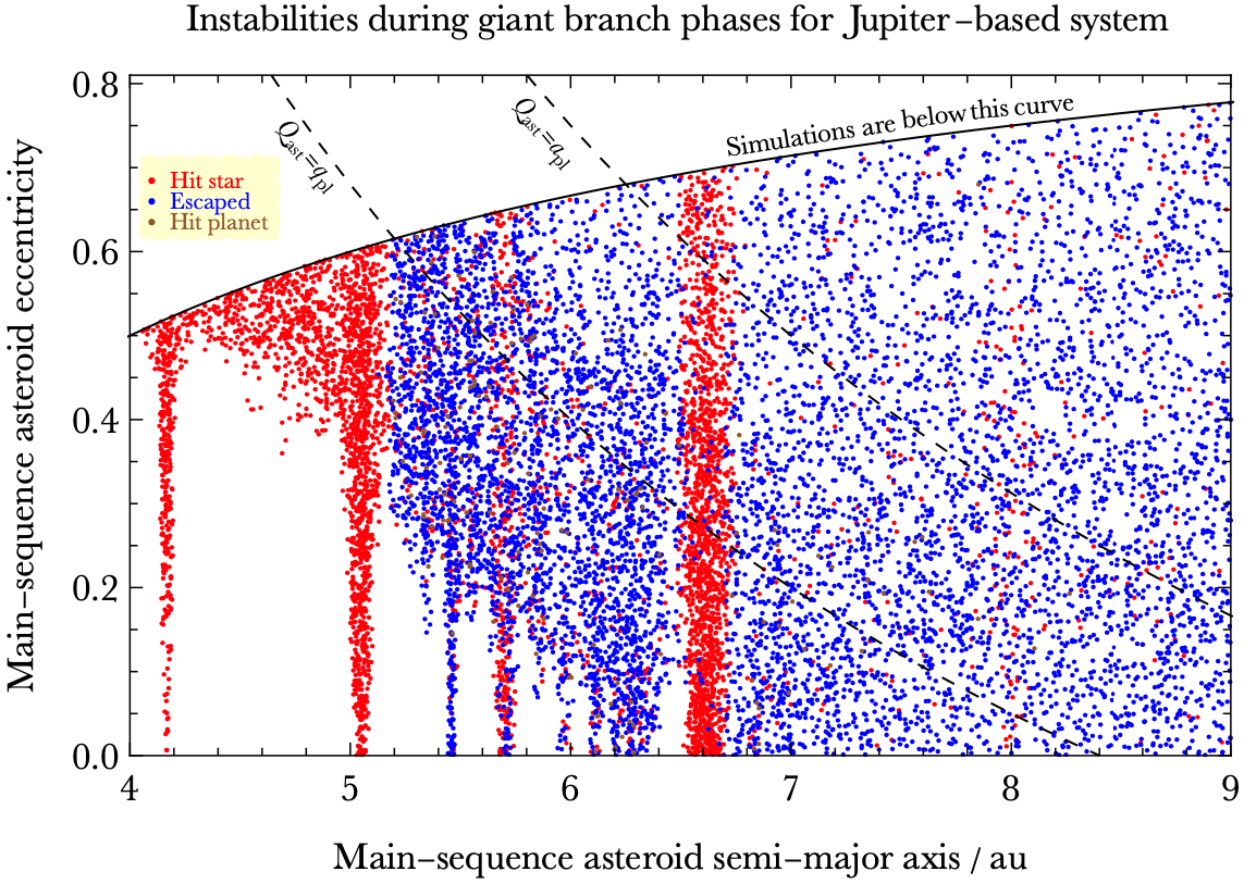
Figure 2: Full resonant instability portraits during the giant branch phases, for the Saturn-based architecture (top) and the Jupiter-based architecture (bottom).

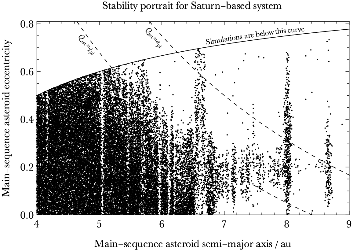
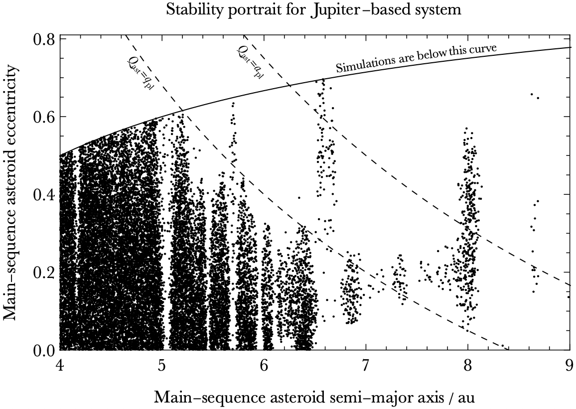
Figure 3: Full resonant stability portraits for the Saturn-based architecture (top) and the Jupiter-based architecture (bottom). All these asteroids remained stable throughout the numerical simulations until they ended, after 1 Gyr of white dwarf cooling. The orbit-crossing curves appear to bound some of the stable regions.

We display the complete instability and stability profiles of our simulations in Figs. 1-3 without yet introducing any markings which are indicative of resonance. In each figure, the top panel is for the system with the Saturn-mass planet, and the bottom panel is for the system with the Jupiter-mass planet.

Figures 1 and 2 identify the asteroids which became unstable during the, respectively, white dwarf and giant branch phases, and Fig. 3 identifies the stable asteroids. In the instability plots, the three colours of dots represent different instability outcomes. We present these profiles, as well as most of the plots in this paper, as a function of both $e_{\rm ast}$ and $a_{\rm ast}$, which represent initial conditions (corresponding to a time which is 10 Myr before the end of the main-sequence).

Each plot contains $3-4$ curves: one solid black, two dashed black, and potentially one solid green. The black solid curve reflects the ($a_{\rm ast},e_{\rm ast}$) boundary above which no asteroids were simulated. The dashed line labelled $Q_{\rm ast}=q_{\rm pl}$ represents the orbit crossing boundary when the arguments of pericentre of the orbits are anti-aligned: above this dashed line, the initial apocentre of the asteroid ($Q_{\rm ast}$) exceeds the initial pericentre of the planet ($q_{\rm pl}$). The dashed line labelled $Q_{\rm ast}=a_{\rm pl}$ instead represents the location where the initial apocentre of the asteroid equals the initial semi-major axis of the planet.

The solid green curve represents an analytical approximation of the close encounter interactions between the planet and the asteroids during the white dwarf phase, where we assume that a close encounter occurs within three times the Hill radius of the pericentre of the planet’s orbit. The curve is hence given by the following function:

$$e_{\rm ast}(a_{\rm ast})=\frac{q_{\rm pl}^{\rm WD}-3R_{\rm Hill}^{\rm WD}}{a_{\rm ast}^{\rm WD}}-1$$

$$\ \ \ \ \ \ \ \ \ \ \ =\frac{\left(\frac{M_{\star}^{\rm MS}}{M_{\star}^{\rm WD}}\right)q_{\rm pl}-3\left(\frac{M_{\star}^{\rm MS}}{M_{\star}^{\rm WD}}\right)^{4/3}R_{\rm Hill}^{\rm MS}}{\left(\frac{M_{\star}^{\rm MS}}{M_{\star}^{\rm WD}}\right)a_{\rm ast}}-1$$

$$\ \ \ \ \ \ \ \ \ \ \ =\frac{q_{\rm pl}}{a_{\rm ast}}\left[1-3^{2/3}\left(\frac{M_{\rm pl}}{M_{\star}^{\rm WD}}\right)^{1/3}\right]-1$$ (1)

where $R_{\rm Hill}^{\rm MS}$ and $R_{\rm Hill}^{\rm WD}$ are the Hill radii of the planet during the main-sequence and white dwarf phases respectively; the 4/3-power relation between these quantities was derived in Payne et al. (2016). Interestingly, equation (1) is independent of $M_{\star}^{\rm MS}$, which may be useful when modelling observed white dwarf planetary systems. All of the curves in Figs. 1-3 will also be drawn in other plots in this paper.

Figures 1-3 have five immediately apparent features. The first is that in almost no case do the asteroids collide with the planet: the instabilities are instead dominated by collisions with the star and escape from the system. The second is that asteroids in the non-resonant regions corresponding to $a_{\rm ast}=6.6-9.0$ au are largely cleared out through escape during the giant branch phases. The third is that for the white dwarf phase, the green solid curves appear to usefully bound some of the unstable regions. The fourth is that asteroids in the non-resonant regions corresponding to $a_{\rm ast}=4.0-6.6$ au remain mostly stable. The fifth is that resonances can act to either stabilize or destablize asteroids. We will quantify these trends in Section 3.6.

Comparing the two plots in each figure reveals other features. The Jupiter-mass planet clears away more asteroids than the Saturn-mass planet, as expected. The orbit-crossing dashed curve appears to play a role in carving out the long-term stability boundaries, despite the initial values of $\omega_{\rm ast}$ being randomized. This dashed curve also serves as a useful demarcation for our subsequent analysis, which now begins with resonances below this curve.

3.2 Resonances for non-crossing orbits

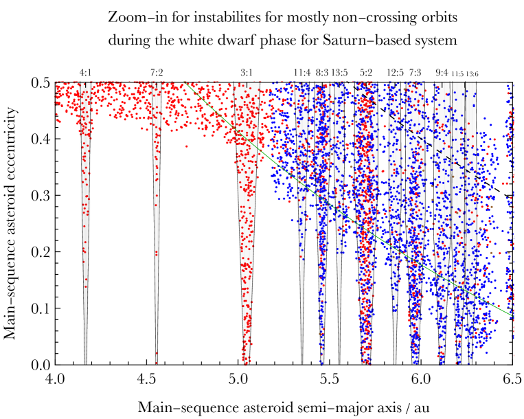
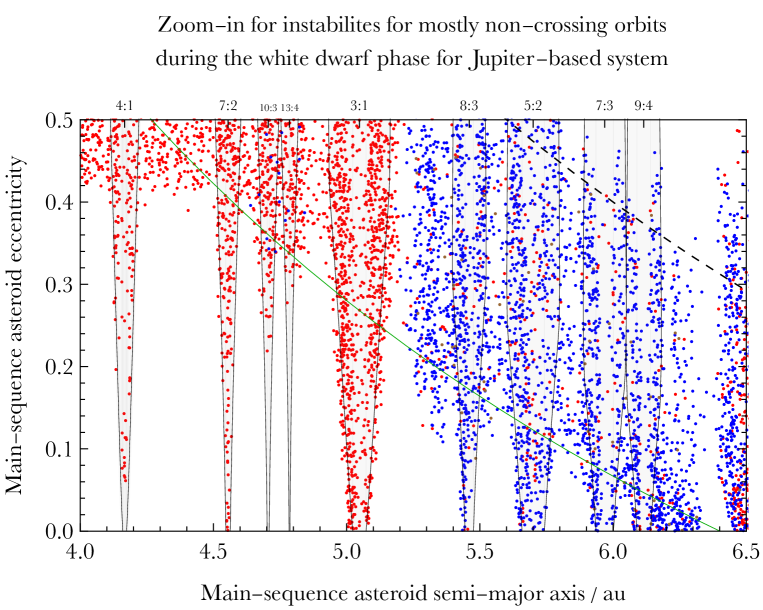
Figure 4: Resonant structures (in light gray shadings) for primarily non-crossing orbits, for the Saturn-based architecture (top) and the Jupiter-based architecture (bottom). The maximum libration widths were computed independently of the $N$-body simulations by integrating with the semi-analytic numerical code of Gallardo et al. (2021). These maximum libration regions are roughly triangular in shape in the non-crossing orbit regime.

Here we focus on resonant structures that are contained within non-crossing orbit regions, which are highlighted in Fig. 4.

The plots in that figure represent zoom-ins of the plots in Fig. 1, with superimposed libration regions represented by the light gray shaded areas and bound by pairs of thin black curves. These libration widths are computed from Gallardo et al. (2021) and actually represent maximum libration widths.

In order to compute these maximum widths, for the star, we assumed a stellar mass of $2.0M_{\odot}$. For the planet, we adopted $a_{\rm pl}=10.5$ au, $e_{\rm pl}=0.2$, and $i_{\rm pl}=\varpi_{\rm pl}=\Omega_{\rm pl}=0^{\circ}$, where $\varpi_{\rm pl}$ represents the longitude of pericentre of the planet. For the asteroid, we chose $a_{\rm pl}$ according to the location of the nominal resonance ($=10.5\,{\rm au}\left(p/q\right)^{-2/3}$, for a $p$:$q$ resonance), and sampled $e_{\rm ast}$ in increments of 0.025. We then fixed $i_{\rm ast}=\Omega_{\rm ast}=0^{\circ}$, but for each value of $e_{\rm ast}$, sampled 180 equally-incremented values of $\varpi_{\rm ast}$ starting at $0^{\circ}$. We finally adopted the maximum width attained from these 180 values, and connected these maximum values at different eccentricities with interpolated curves.

Therefore, the computation of maximum libration widths did not explicitly take into account stellar evolution or the evolution of the asteroid’s orbital parameters. Nevertheless, this method of computing maximum libration widths with just main-sequence values appears to be effective when compared to the results of the $N$-body simulations – which are completely independent from the code used to compute the libration widths.

As can be seen, these widths accurately reflect the resonant influences that are indicated by the outcome of the $N$-body simulations. These widths all monotonically increase with $e_{\rm ast}$ until around the eccentricity value where the orbits cross (the dashed line). Around this location, the widths become nearly fixed or slightly decrease for greater $e_{\rm ast}$. How reflective this structure is of the actual physical evolution is difficult to determine because at high values of $e_{\rm ast}$, resonant overlap occurs more readily and the unstable asteroids are sparse and do not form a coherent structure.

For crossing orbits, the libration widths are dependent on the close encounter criterion set in the Gallardo et al. (2021) code through the parameter rhtol. Gallardo (2020) found that an accurate value for this close encounter criterion in the restricted three-body problem is three planetary Hill radii (rhtol $=3$), which we adopted here. We also performed extensive tests with rhtol $=0$ and confirmed that while the libration widths with that value do not differ much for $e_{\rm ast}$ below the collision curve, above the collision curve widths become unrealistic and do not reflect the outcome of our $N$-body simulations.

Comparing the two plots in Fig. 4 reveals that during the white dwarf phase, the influence of some resonances vanish when the planetary mass changes; only resonances which have a discernible effect on the dynamics are plotted. For example, during this phase of stellar evolution, the Jupiter-mass planet apparently accessed pollution reservoirs at the 7th- and 9th-order resonances $10$:$3$ and $13$:$4$; such reservoirs are not easily identifiable for the Saturn-mass planet architecture.

3.3 The $2$:$1$ resonance

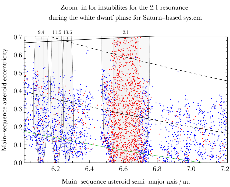
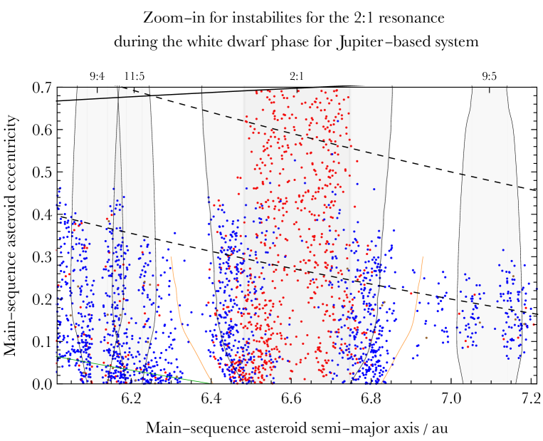
Figure 5: The $2$:$1$ resonant structures for the Saturn-based (top) and Jupiter-based (bottom) architectures. In the orbit-crossing regime (above the lower dashed curve) the semianalytic maximum libration structure stops increasing monotonically with $e_{\rm ast}$. The $2$:$1$ resonant core (the slightly darker gray regions) usefully separate white dwarf pollutants from escapers at high $e_{\rm ast}$.

We next zoom into the region surrounding the $2$:$1$ resonance, in Fig. 5. This resonance deserves special attention both because of its strength – being a first-order resonance – and because it has been highlighted in previous post-main-sequence resonance studies. Also, Fig. 1 indicates immediately that the $2$:$1$ resonance is a significant driver of white dwarf pollution.

In Fig. 5, there are resonant structures which are immediately apparent aside from the $2$:$1$ resonance. Libration widths for these other resonances have been computed and displayed on the plots, although their influence is clear primarily in the non-crossing orbit regime. For the $2$:$1$ resonance, for the planetary architecture that we adopted, crossing orbits occur when $e_{\rm ast}\gtrsim 0.27$.

We see structure on both sides of this eccentricity boundary. For $e_{\rm ast}\lesssim 0.27$, the computed maximum libration width region does provide a qualitatively-good bound on resonant behaviour, but does appear to slightly underestimate the true region of influence.

One potential reason for the underestimation is that the resonance width computed here does not take into account stellar evolution. When the star-to-planet mass ratio changes, the libration width should change also. Debes et al. (2012) explicitly drew this change for the $2$:$1$ resonance by using the formula for libration width from Murray & Dermott (1999), which does not incorporate as many input parameters as the semianalytical prescription from Gallardo et al. (2021).

Hence, as an exploratory exercise, for the Jupiter-based system, we recomputed the maximum libration width with the Gallardo et al. (2021) prescription, but instead adopted the white dwarf mass of $0.637M_{\odot}$ instead of the main-sequence mass of $2.0M_{\odot}$. We drew the result as a pair of thin superimposed solid orange curves on the bottom plot of Fig. 5. These curves, however, appear to significantly overestimate the region of influence of the resonance for $e_{\rm ast}\gtrsim 0.05$.

Returning to our original computation of libration width, the instability types suggest that we may usefully split the resonant region above the orbit-crossing curve into a “core” and a “tail”. We define the core as the width computed at $e_{\rm ast}=0$ as applied to all $e_{\rm ast}$, as indicated by the slightly darker gray region. The tail is then defined as the region outside of the core but bounded by libration width boundaries.

With these definitions, a visual inspection of the plot immediately indicates that $2$:$1$ asteroids which pollute the white dwarf are located in the resonant core, and those which escape the system are located in the tails. This trend appears to continue even in the crossing-orbit regime ($e_{\rm ast}\geq 0.27$) except that the locations of the asteroids which feature escape stick to the boundaries of the core before vanishing entirely above some critical eccentricity. These trends hold for both the Jupiter-mass and Saturn-mass cases.

The physical explanation for this behaviour is that only those asteroids which are deep enough in the resonance (in the core) can secularly evolve such that their eccentricities are increased to near-unity while their semi-major axes remain nearly constant. Alternatively, asteroids that are on the edge of the resonance (in the tails) more easily escape the resonance and subsequently experience encounters with the planet, allowing their semi-major axes to be periodically pumped until ejection.

3.4 The $3$:$2$ and $4$:$3$ resonances

Next, we zoom-in to the rightmost portion of Figs. 1 and 3 in Fig. 6, which features asteroids that are almost exclusively in the crossing-orbit regime. Here, for the two first-order resonances, the maximum libration width computed from the Gallardo et al. (2021) prescription does not increase monotonically with $e_{\rm ast}$, but rather does just the opposite.

The distribution of both unstable and stable asteroids which are illustrated in the figure strongly suggest that both the $3$:$2$ and $4$:$3$ resonances have played a role in the asteroids’ dynamical evolution. The $3$:$2$ resonance appears to have exerted influence on asteroids with higher values of $e_{\rm ast}$ than the $4$:$3$ resonance. Both resonance regions include a mixture of asteroids which pollute the white dwarf, and those which escape from the system during the white dwarf phase.

The bottom panel of Fig. 6 is notable for how it demonstrates that asteroids can be protected from instability through different stages of stellar evolution by being trapped into a strong resonance. The plot also shows how such asteroids are more likely to be protected for low values of $e_{\rm ast}$, even though a few remain stable at nearly the highest values of $e_{\rm ast}$ sampled.

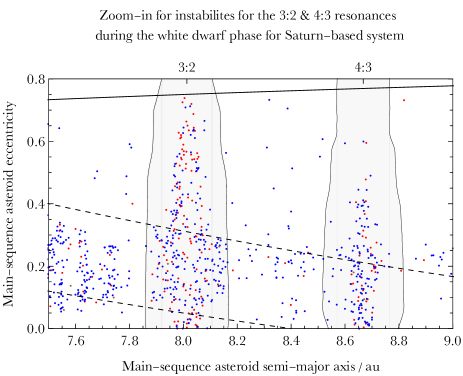
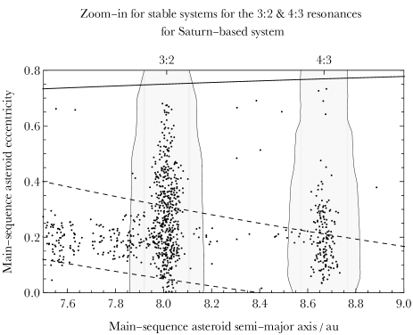
Figure 6: Influence of the $3$:$2$ and $4$:$3$ resonances, which are located almost entirely in the crossing-orbit regime, on instability location during the white dwarf phase (top panel) and on maintaining stability (bottom panel). Both resonances clearly influence the stability portraits across the sampled parameter space.

3.5 Libration width comparisons

We have now shown, by comparison with $N$-body simulations, that the maximum libration regions computed with main-sequence values may be sufficiently accurate to be used as reliable proxies for the initial location of post-main-sequence resonant dynamical behaviour. In this subsection, we explore in more detail how these maximum libration widths vary depending on the input parameters which are adopted. All plots in this section show $N$-body simulation output from the white dwarf phase only.

First, we tested the sensitivity of our maximum libration width computations on the sampling frequency of $\varpi_{\rm ast}$. So far, we have computed widths for each of 180 equally-spaced values of $\varpi_{\rm ast}$, and then drew output corresponding to the maximum of these widths. Figure 7 illustrates the result of reducing this sampling rate for the $3$:$1$ resonance in the Saturn-based system.

On the figure, we drew five different pairs of curves corresponding to sampling rates of 180, 72, 36, 18 and 1 value. The differences between the first four pairs of curves are not discernible for most of the non-orbit crossing regime, helping to illustrate the robustness of our fiducial choice for the plots in this paper. However, when we sampled just a single value of $\varpi_{\rm ast}$, in this case $\varpi_{\rm ast}=0^{\circ}$, the result differs, as shown by the middle pair of curves.

Overall then, this example demonstrates that adopting a single value of $\varpi_{\rm ast}$ produces a quantitatively different, and more inaccurate, result than sampling multiple values and taking the maximum output. Further, the results of our $N$-body simulations demonstrate that the libration region in the non-orbit crossing regime increases monotonically with $e_{\rm ast}$, and does not curve inward at $e_{\rm ast}=0.05$, as indicated by the $\varpi_{\rm ast}=0^{\circ}$ curve.

In order to fortify these conclusions, we performed the same exercise for the $2$:$1$ resonance. The result is shown in Fig. 8, and is the same: the shape of the curves resulting from the fixed value of $\varpi_{\rm ast}=0^{\circ}$ does not reflect the region of influence from the $N$-body simulations, and here significantly underestimates the number of asteroids under this influence.

Because the libration width prescription of Gallardo et al. (2021) requires a full set of three-dimension orbital inputs for both the asteroid and planet, and because all orbital elements of the asteroids varied throughout our simulations, we then explored how these libration curves change by varying $i_{\rm ast}$ and $\Omega_{\rm ast}$. The result is shown in Fig. 9.

Illustrated in this figure are 8 different pairs of maximum libration width curves, some of which overlap, that correspond to ($i_{\rm ast}$, $\Omega_{\rm ast}$) = ($0^{\circ}$, $0^{\circ}$), ($5^{\circ}$, $0^{\circ}$), ($20^{\circ}$, $0^{\circ}$), ($20^{\circ}$, $180^{\circ}$), ($50^{\circ}$, $0^{\circ}$), ($50^{\circ}$, $90^{\circ}$), ($50^{\circ}$, $180^{\circ}$) and ($50^{\circ}$, $270^{\circ}$). All of these curves do present shapes which are reflective of the results of the $N$-body simulations, but with slightly different tails.

For asteroids that pollute the white dwarf, we expect that the extent of the isotropy with which asteroids enter the white dwarf’s Roche radius to increase with planet mass (Veras et al., 2021). Hence, for particularly massive planets, we might obtain more accurate bounds on the libration region by sampling multiple values of $i_{\rm ast}$, $\Omega_{\rm ast}$ and $\varpi_{\rm ast}$, rather than just $\varpi_{\rm ast}$. However, doing so would become computationally expensive.

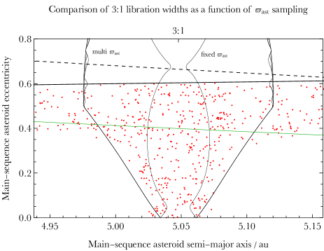
Figure 7: Result of computing maximum libration widths for the $3$:$1$ resonance with five different sampling frequencies for $\varpi_{\rm ast}$ (with 180, 72, 36, 18, 1 values sampled, starting at $0^{\circ}$). This plot illustrates that the maximum libration width is largely independent of sampling frequency. However, adopting a fixed value of $\varpi_{\rm ast}$ generates a qualitatively differently-shaped region (middle pair of curves).

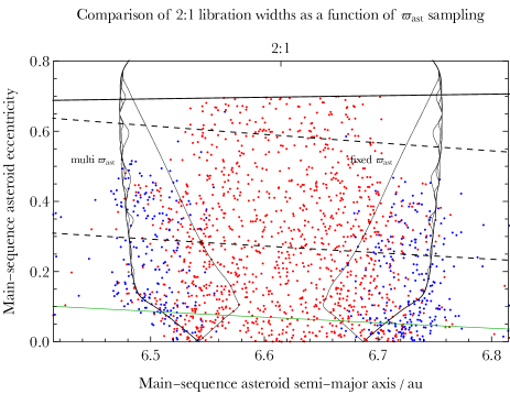
Figure 8: Similar to Fig. 7, except for the $2$:$1$ resonance, where the result of adopting a fixed value of $\varpi_{\rm ast}$ is more pronounced and would lead to a more significant underestimation of the number of asteroids which are influenced by this resonance.

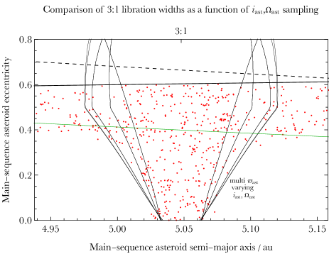
Figure 9: Result of computing maximum libration widths for the $3$:$1$ resonance with different initial values of ($i_{\rm ast}$, $\Omega_{\rm ast}$). The different pairs adopted, in addition to the nominal pair ($0^{\circ}$, $0^{\circ}$), were ($5^{\circ}$, $0^{\circ}$), ($20^{\circ}$, $0^{\circ}$), ($20^{\circ}$, $180^{\circ}$), ($50^{\circ}$, $0^{\circ}$), ($50^{\circ}$, $90^{\circ}$), ($50^{\circ}$, $180^{\circ}$) and ($50^{\circ}$, $270^{\circ}$).

Table 1: Simulation outcomes for selected resonant regions; WD stands for white dwarf and GB stands for giant branch. Included are all 1st- to 5th-order resonances between the $4$:$1$ and $2$:$1$ inclusive, as well as the $3$:$2$ and $4$:$3$ resonances, which are both deep into the crossing orbit regime. The value of $a_{\rm ast,nom}$ represents the asteroid’s nominal initial location for each resonance. The underlined values in the fourth column highlight relatively efficient white dwarf polluters (the $2$:$1$, $3$:$1$ and $4$:$1$ resonances).

Resonance	$a_{\rm ast,nom}$	Total	WD	WD	WD	GB	GB	GB	Stable
	/ au	Number	Hit star	Escaped	Hit planet	Hit star	Escaped	Hit Planet
$4$:$1$ Saturn	4.17	531	$\underline{21\%}$	$0\%$	$0\%$	$14\%$	$0\%$	$0\%$	$55\%$
$4$:$1$ Jupiter	4.17	1014	$\underline{32\%}$	$0\%$	$0\%$	$16\%$	$0\%$	$0\%$	$41\%$
$7$:$2$ Saturn	4.55	543	$5.3\%$	$0\%$	$0\%$	$13\%$	$0\%$	$0\%$	$81\%$
$7$:$2$ Jupiter	4.55	900	$7.1\%$	$0\%$	$0\%$	$31\%$	$0\%$	$0\%$	$60\%$
$3$:$1$ Saturn	5.05	1666	$\underline{24\%}$	$0\%$	$0\%$	$24\%$	$0\%$	$0\%$	$40\%$
$3$:$1$ Jupiter	5.05	2986	$\underline{36\%}$	$0.033\%$	$0\%$	$33\%$	$0.033\%$	$0\%$	$16\%$
$8$:$3$ Saturn	5.46	1187	$8.6\%$	$2.8\%$	$0.08\%$	$14\%$	$33\%$	$0.25\%$	$32\%$
$8$:$3$ Jupiter	5.46	1886	$5.9\%$	$22\%$	$0.80\%$	$2.2\%$	$19\%$	$0.42\%$	$14\%$
$5$:$2$ Saturn	5.70	2102	$8.2\%$	$4.0\%$	$0.29\%$	$25\%$	$22\%$	$0.24\%$	$31\%$
$5$:$2$ Jupiter	5.70	3234	$10\%$	$14\%$	$0.56\%$	$3.5\%$	$17\%$	$0.093\%$	$14\%$
$7$:$3$ Saturn	5.97	1803	$13\%$	$14\%$	$0.50\%$	$8.4\%$	$22\%$	$0.44\%$	$16\%$
$7$:$3$ Jupiter	5.97	2642	$2.2\%$	$12\%$	$0.26\%$	$1.3\%$	$11\%$	$0.26\%$	$9.0\%$
$9$:$4$ Saturn	6.11	1506	$13\%$	$21\%$	$0.86\%$	$3.1\%$	$16\%$	$0.13\%$	$12\%$
$9$:$4$ Jupiter	6.11	2328	$2.2\%$	$14\%$	$0.34\%$	$1.5\%$	$11\%$	$0.21\%$	$5.4\%$
$2$:$1$ Saturn	6.61	5295	$\underline{27\%}$	$7.3\%$	$0.23\%$	$21\%$	$4.9\%$	$0.019\%$	$12\%$
$2$:$1$ Jupiter	6.61	8787	$\underline{18\%}$	$4.3\%$	$0.057\%$	$8.2\%$	$5.6\%$	$0.023\%$	$3.4\%$
$3$:$2$ Saturn	8.01	6084	$7.1\%$	$18\%$	$0.23\%$	$1.9\%$	$3.4\%$	$0.033\%$	$9.1\%$
$3$:$2$ Jupiter	8.01	9619	$1.3\%$	$6.8\%$	$0.031\%$	$0.32\%$	$2.5\%$	$0.010\%$	$4.0\%$
$4$:$3$ Saturn	8.67	5873	$5.9\%$	$23\%$	$0.10\%$	$0.63\%$	$2.1\%$	$0.034\%$	$2.9\%$
$4$:$3$ Jupiter	8.67	8881	$0.53\%$	$7.1\%$	$0\%$	$0.14\%$	$1.1\%$	$0.011\%$	$0.17\%$

3.6 Resonant outcomes and strengths

So far, the plots in this paper have illustrated different instability outcomes for different resonances. In this subsection, we tabulate these results for selected resonances in Table 1.

The resonances (1st column) are ordered by horizontal location on Figs. 1-3 (second column). The third column reports the total number of asteroids initially contained within that resonant region. This number also includes those asteroids that have been cleared out during the first 10 Myr with a fixed stellar mass in order to allow the system to dynamically settle, at least to a minor extent.

The remaining columns report the outcomes of the simulations in percentages of the initial asteroid sample ( third column), with highlighted results underlined in the fourth column. The table illustrates the following trends:

1. The most significant polluters of white dwarfs arise from the $2$:$1$, $3$:$1$ and $4$:$1$ resonances, with at least 18 per cent of the asteroids in each of those resonant regions entering the Roche radius of the star. By way of comparison with another third-order resonance in the non-orbit crossing regime – the $5$:$2$ – the $4$:$1$ is a much more efficient polluter. This result supports the finding that the $4$:$1$ resonance can easily excite test particles to high eccentricity in the presence of a slightly eccentric planet (Pichierri et al., 2017).

2. A different measure of the efficiency of the $2$:$1$, $3$:$1$ and $4$:$1$ resonances to pollute the white dwarf is by comparison to the total number of polluters across our entire initial disc of asteroids. Although such a comparison is highly dependent on our choice of the inner and outer edges of the initial disc, this comparison may still be useful. For the Saturn-based and Jupiter-based systems, respectively, approximately $47$ and $80$ per cent of all polluters were generated from the $2$:$1$, $3$:$1$ and $4$:$1$ resonances. More specifically, for the Saturn-based system, each of these resonances provided respectively $35$, $9.6$ and $2.7$ per cent of pollutants, whereas for the Jupiter-based system, the percentages were $42$, $29$ and $8.6$.

3. Resonances can stabilise asteroids, even those in crossing orbits (the $4$:$3$ and $3$:$2$), and sometimes in large quantities (tens of per cent of the original reservoir). These stable populations are also potentially important for white dwarf pollution, particularly at late times (beyond 1 Gyr of white dwarf cooling) because they may be (a) accessed later by external perturbers which initially played no role in the dynamics within tens of au (Bonsor & Veras, 2015; Veras et al., 2016), or, (b) when close enough to the white dwarf, dragged into the star from its own radiation (Rafikov, 2011; Veras et al., 2015b, 2022; Veras, 2020; Malamud et al., 2021; Brouwers et al., 2022).

4. Escape from the system is more difficult, if not impossible, from resonant regions close to the star. In this region close asteroid encounters with the planet are non-existent; such encounters would be required for an asteroid to be ejected.

5. Asteroid collisions with the planet are rare in all cases. The three resonances which produce the greatest fraction of these types of collisions are the 4th- and 5th-order resonances $9$:$4$, $8$:$3$ and $7$:$3$, but only at the 1 per cent level.

In an attempt to quantify the strength of various resonances, we used a numerical strength measure from the semianalytic prescription that was defined in equation 8 of Gallardo (2006) as a difference in disturbing function evaluations, computed numerically (not with expansions). We then normalized this numerical strength measure for selected resonances as a function of $e_{\rm ast}$, and show the results in Fig. 10.

That plot illustrates that in the non-crossing orbit regime, strength varies smoothly with $e_{\rm ast}$. Also, the differences in strength are most pronounced for asteroids on low-eccentricity orbits. This strength metric usefully takes into account both resonant order and proximity to the planet, but does not trace secular evolution, the results of which are presented in Table 1.

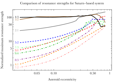
Figure 10: Relative strengths of different resonances as a function of $e_{\rm ast}$ for the Saturn-based system. The plot for the Jupiter-based system is equivalent, except for strengths which are scaled up by a factor of 3.34. The strengths are computed according to the prescription in Gallardo (2006). On this plot, the 1st-order resonances are given by solid curves, 2nd-order and 3rd-order resonances by dashed curves, and 4th-order and 5th-order resonances by dot-dashed curves. The curves are smooth and monotonically increasing with $e_{\rm ast}$ in the non-crossing orbit regime.

4 Discussion

The results of this investigation not only have intrinsic dynamical interest, but also may be applied to individual real systems in the near future, especially as more suitable one-planet polluted white dwarf systems are discovered. Right now no systems are confirmed as such, but we are at least aware of a near Jovian-analogue in planet-star separation and mass with MOA-2010-BLG-477L b (Blackman et al., 2021). If that star is shown to be polluted, then we might be able to make qualitative statements about the role mean motion resonances are playing in that system’s dynamical evolution.

The high computational expense of our simulations precludes a wider exploration of parameter space in this investigation. Amongst our “wish list” of potential extensions to this investigation include considering an interior, rather than exterior, planet, and determining how to scale down the mass of the planet while scaling up the resolution in order to still be able to detect resonant signatures. Veras et al. (2021) did perform a wider parameter space, but at a much lower resolution.

Our results here also may aid investigations which derive eccentric-orbit stability boundary and timescale criteria (Georgakarakos, 2008; Petit et al., 2018), as well as chaos-triggering and resonant overlap criteria (Quillen, 2011; Mustill & Wyatt, 2012; Deck et al., 2013; Hadden & Lithwick, 2018; Petit et al., 2020; Tamayo et al., 2021; Rath et al., 2022), and determine how these criteria might change with mass shifts as the star evolves.

What we have integrated here is many instances of the eccentric, non-coplanar restricted three-body problem with mass loss. However, as suggested by Ramos et al. (2015), this scenario is complex-enough to not necessarily be well-characterized by a single class of dynamical measures (e.g. Hill stability, Lagrange stability, angular momentum deficit, chaotic zone boundaries, resonance overlap). For example, none of the stable $4$:$3$ systems are Hill stable, and many of the resonant overlap investigations cited above assume circular orbits and multiple massive planets.

Indeed, one potential extension of this work is to include a second planet into our simulations. Then, secular resonances might become prominent, and the studies of Smallwood et al. (2018) and Smallwood et al. (2021) may better be used as a benchmark for comparison. Perhaps though the most physically important extension to these simulations would be to model the radiative effect on the test particles. Our results here hold only when the test particles are large enough ($\gtrsim 10^{3}$ km) to remain unaffected. Smaller debris would instead move about significantly during the simulations from stellar radiation alone (Bonsor & Wyatt, 2010; Dong et al., 2010; Veras et al., 2015a, 2019; Zotos & Veras, 2020; Ferich et al., 2022).

5 Summary

We have produced high-resolution resonant portraits (Figs. 1-3) of an evolved one-planet system with $10^{5}$ asteroids, and compared the $N$-body simulation results to a semi-analytical libration width calculator (Gallardo et al., 2021) that does not rely on traditional disturbing function expansions and allows for full three-dimensional inputs. These portraits include regimes of both crossing and non-crossing orbits, and provide insight into the escape, pollution and stability efficiencies of different resonances at different stages of stellar evolution (Table 1). Our maximum libration width computations are robust (e.g. Fig. 7) and usefully show (e.g. Fig. 4) that we can use main-sequence values to accurately determine the domain of influence of different resonances – saving time and computational resources for future resonance-based investigations of evolved planetary systems.

Data Availability

The simulation inputs and results discussed in this paper are available upon reasonable request to the corresponding author.

References

- Antoniadou & Veras (2016) Antoniadou, K. I., & Veras, D. 2016, MNRAS, 463, 4108
- Antoniadou & Veras (2019) Antoniadou, K. I., & Veras, D. 2019, A&A, 629, A126
- Blackman et al. (2021) Blackman, J. W., Beaulieu, J. P., Bennett, D. P., et al. 2021, Nature, 598, 272.
- Bonsor & Wyatt (2010) Bonsor, A., & Wyatt, M. 2010, MNRAS, 409, 1631
- Bonsor et al. (2011) Bonsor, A., Mustill, A. J., & Wyatt, M. C. 2011, MNRAS, 414, 930
- Bonsor & Veras (2015) Bonsor, A., & Veras, D. 2015, MNRAS, 454, 53
- Bonsor et al. (2017) Bonsor, A., Farihi, J., Wyatt, M. C., & van Lieshout, R. 2017, MNRAS, 468, 154
- Brouwers et al. (2022) Brouwers, M. G., Bonsor, A., & Malamud, U. 2022, MNRAS, 509, 2404.
- Brown et al. (2017) Brown, J. C., Veras, D., & Gänsicke, B. T. 2017, MNRAS, 468, 1575
- Buchan et al. (2022) Buchan, A. M., Bonsor, A., Shorttle, O., et al. 2022, MNRAS, 510, 3512.
- Caiazzo & Heyl (2017) Caiazzo, I., & Heyl, J. S. 2017, MNRAS, 469, 2750.
- Chamandy et al. (2021) Chamandy, L., Blackman, E. G., Nordhaus, J., et al. 2021, MNRAS, 502, L110.
- Cunningham et al. (2022) Cunningham, T., Wheatley, P. J., Tremblay, P.-E., et al. 2022, Nature, 602, 219.
- Curry et al. (2022) Curry, A., Bonsor, A., Lichtenberg, T., et al. 2022, MNRAS, 515, 395.
- Debes & Sigurdsson (2002) Debes, J. H., & Sigurdsson, S. 2002, ApJ, 572, 556
- Debes et al. (2012) Debes, J. H., Walsh, K. J., & Stark, C. 2012, ApJ, 747, 148
- Deck et al. (2013) Deck, K. M., Payne, M., & Holman, M. J. 2013, ApJ, 774, 129.
- Dermott et al. (2021) Dermott, S. F., Li, D., Christou, A. A., et al. 2021, MNRAS, 505, 1917.
- Dong et al. (2010) Dong, R., Wang, Y., Lin, D. N. C., & Liu, X.-W. 2010, ApJ, 715, 1036
- Dosopoulou & Kalogera (2016a) Dosopoulou, F. & Kalogera, V. 2016a, ApJ, 825, 70.
- Dosopoulou & Kalogera (2016b) Dosopoulou, F. & Kalogera, V. 2016b, ApJ, 825, 71.
- Doyle et al. (2019) Doyle, A. E., Young, E. D., Klein, B., et al. 2019, Science, 366, 356
- Doyle et al. (2021) Doyle, A. E., Desch, S. J., & Young, E. D. 2021, ApJL, 907, L35.
- Farihi et al. (2013) Farihi, J., Gänsicke, B. T., & Koester, D. 2013, Science, 342, 218.
- Farihi (2016) Farihi, J. 2016, New Astronomy Reviews, 71, 9
- Ferich et al. (2022) Ferich, N., Baronett, S. A., Tamayo, D., et al. 2022, ApJS, 262, 41.
- Frewen & Hansen (2014) Frewen, S. F. N., & Hansen, B. M. S. 2014, MNRAS, 439, 2442
- Gaia Collaboration et al. (2022) Gaia Collaboration, Arenou, F., Babusiaux, C., et al. 2022, arXiv:2206.05595, In Press, A&A
- Gallardo (2006) Gallardo, T. 2006, Icarus, 184, 29.
- Gallardo (2019) Gallardo, T. 2019, Icarus, 317, 121.
- Gallardo (2020) Gallardo, T. 2020, Celestial Mechanics and Dynamical Astronomy, 132, 9.
- Gallardo et al. (2021) Gallardo, T., Beaugé, C., & Giuppone, C. A. 2021, A&A, 646, A148.
- Gänsicke et al. (2012) Gänsicke, B. T., Koester, D., Farihi, J., et al. 2012, MNRAS, 424, 333
- Gänsicke et al. (2019) Gänsicke, B. T., Schreiber, M. R., Toloza, O., et al. 2019, Nature, 576, 61
- Gentile Fusillo et al. (2017) Gentile Fusillo, N. P., Gänsicke, B. T., Farihi, J., et al. 2017, MNRAS, 468, 971.
- Georgakarakos (2008) Georgakarakos, N. 2008, Celestial Mechanics and Dynamical Astronomy, 100, 151.
- Grunblatt et al. (2018) Grunblatt, S. K., Huber, D., Gaidos, E., et al. 2018, ApJL, 861, L5.
- Grunblatt et al. (2022) Grunblatt, S. K., Saunders, N., Chontos, A., et al. 2022, Submitted to ApJ
- Hadden & Lithwick (2018) Hadden, S. & Lithwick, Y. 2018, AJ, 156, 95.
- Hadjidemetriou (1963) Hadjidemetriou, J. D. 1963, Icarus, 2, 440
- Hamers & Portegies Zwart (2016) Hamers A. S., Portegies Zwart S. F., 2016, MNRAS, 462, L84
- Hoskin et al. (2020) Hoskin, M. J., Toloza, O., Gänsicke, B. T., et al. 2020, MNRAS, 499, 171.
- Hurley et al. (2000) Hurley, J. R., Pols, O. R., & Tout, C. A. 2000, MNRAS, 315, 543.
- Jura (2003) Jura, M. 2003, ApJL, 584, L91
- Jura & Young (2014) Jura, M., & Young, E. D. 2014, Annual Review of Earth and Planetary Sciences, 42, 45
- Klein et al. (2021) Klein, B. L., Doyle, A. E., Zuckerman, B., et al. 2021, ApJ, 914, 61.
- Koester et al. (2014) Koester, D., Gänsicke, B. T., & Farihi, J. 2014, A&A, 566, A34.
- Kunitomo et al. (2011) Kunitomo, M., Ikoma, M., Sato, B., Katsuta, Y., & Ida, S. 2011, ApJ, 737, 66
- Lagos et al. (2021) Lagos, F., Schreiber, M. R., Zorotovic, M., et al. 2021, MNRAS, 501, 676.
- Li et al. (2021) Li, D., Mustill, A. J., & Davies, M. B. 2021, MNRAS, 508, 5671.
- Li et al. (2022) Li, D., Mustill, A. J., & Davies, M. B. 2022, ApJ, 924, 61.
- Luhman et al. (2011) Luhman, K. L., Burgasser, A. J., & Bochanski, J. J. 2011, ApJL, 730, L9.
- Madappatt et al. (2016) Madappatt, N., De Marco, O., & Villaver, E. 2016, MNRAS, 463, 1040
- Malamud & Perets (2020a) Malamud, U. & Perets, H. B. 2020a, MNRAS, 492, 5561
- Malamud & Perets (2020b) Malamud, U. & Perets, H. B. 2020b, MNRAS, 493, 698.
- Malamud et al. (2021) Malamud, U., Grishin, E., & Brouwers, M. 2021, MNRAS, 501, 3806.
- Maldonado et al. (2021) Maldonado, R. F., Villaver, E., Mustill, A. J., et al. 2021, MNRAS, 501, L43.
- Manser et al. (2020) Manser, C. J., Gänsicke, B. T., Gentile Fusillo, N. P., et al. 2020, MNRAS, 493, 2127
- McDonald & Veras (2021) McDonald, C. H. & Veras, D. 2021, MNRAS, 506, 4031.
- Melis & Dufour (2017) Melis, C. & Dufour, P. 2017, ApJ, 834, 1.
- Moro-Martín (2022) Moro-Martín, A. 2022, arXiv:2205.04277
- Muñoz & Petrovich (2020) Muñoz, D. J. & Petrovich, C. 2020, ApJL, 904, L3.
- Murray & Dermott (1999) Murray, C. D. & Dermott, S. F. 1999, Solar system dynamics by C.D. Murray and S.F. McDermott. (Cambridge, UK: Cambridge University Press), ISBN 0-521-57295-9 (hc.), ISBN 0-521-57297-4 (pbk.).
- Mustill & Villaver (2012) Mustill, A. J., & Villaver, E. 2012, ApJ, 761, 121
- Mustill & Wyatt (2012) Mustill, A. J. & Wyatt, M. C. 2012, MNRAS, 419, 3074.
- Mustill et al. (2014) Mustill, A. J., Veras, D., & Villaver, E. 2014, MNRAS, 437, 1404
- Mustill et al. (2018) Mustill, A. J., Villaver, E., Veras, D., Gänsicke, B. T., Bonsor, A. 2018, MNRAS, 476, 3939.
- Nordhaus & Spiegel (2013) Nordhaus, J., & Spiegel, D. S. 2013, MNRAS, 432, 500
- O’Connor & Lai (2020) O’Connor, C. E. & Lai, D. 2020, MNRAS, 498, 4005.
- O’Connor et al. (2022) O’Connor, C. E., Teyssandier, J., & Lai, D. 2022, MNRAS, 513, 4178.
- Omarov (1962) Omarov, T. B. 1962, Izv. Astrofiz. Inst. Acad. Nauk. KazSSR, 14, 66
- Payne et al. (2016) Payne, M. J., Veras, D., Holman, M. J., Gänsicke, B. T. 2016, MNRAS, 457, 217
- Petit et al. (2018) Petit, A. C., Laskar, J., & Boué, G. 2018, A&A, 617, A93.
- Petit et al. (2020) Petit, A. C., Pichierri, G., Davies, M. B., et al. 2020, A&A, 641, A176.
- Petrovich & Muñoz (2017) Petrovich, C., & Muñoz, D. J. 2017, ApJ, 834, 116
- Pichierri et al. (2017) Pichierri, G., Morbidelli, A., & Lai, D. 2017, A&A, 605, A23.
- Quillen (2011) Quillen, A. C. 2011, MNRAS, 418, 1043.
- Raddi et al. (2015) Raddi, R., Gänsicke, B. T., Koester, D., et al. 2015, MNRAS, 450, 2083.
- Rafikov (2011) Rafikov, R. R. 2011, ApJL, 732, L3
- Ramos et al. (2015) Ramos, X. S., Correa-Otto, J. A., & Beaugé, C. 2015, Celestial Mechanics and Dynamical Astronomy, 123, 453.
- Rath et al. (2022) Rath, J., Hadden, S., & Lithwick, Y. 2022, ApJ, 932, 61.
- Rocchetto et al. (2015) Rocchetto, M., Farihi, J., Gänsicke, B. T., et al. 2015, MNRAS, 449, 574
- Ronco et al. (2020) Ronco, M. P., Schreiber, M. R., Giuppone, C. A., et al. 2020, ApJL, 898, L23.
- Sigurdsson et al. (2003) Sigurdsson, S., Richer, H. B., Hansen, B. M., et al. 2003, Science, 301, 193.
- Smallwood et al. (2018) Smallwood, J. L., Martin, R. G., Livio, M., & Lubow, S. H. 2018, MNRAS, 480, 57
- Smallwood et al. (2021) Smallwood, J. L., Martin, R. G., Livio, M., et al. 2021, MNRAS, 504, 3375.
- Stephan et al. (2017) Stephan, A. P., Naoz, S., & Zuckerman, B. 2017, ApJL, 844, L16
- Stephan et al. (2021) Stephan, A. P., Naoz, S., & Gaudi, B. S. 2021, ApJ, 922, 4.
- Swan et al. (2019) Swan, A., Farihi, J., Koester, D., et al. 2019, MNRAS, 490, 202
- Szölgyén et al. (2022) Szölgyén, Á., MacLeod, M., & Loeb, A. 2022, MNRAS, 513, 5465.
- Tamayo et al. (2021) Tamayo, D., Murray, N., Tremaine, S., et al. 2021, AJ, 162, 220.
- Thorsett et al. (1993) Thorsett, S. E., Arzoumanian, Z., & Taylor, J. H. 1993, ApJL, 412, L33.
- Vanderburg et al. (2020) Vanderburg, A., Rappaport, S. A., Xu, S., et al. 2020, Nature, 585, 363.
- Veras et al. (2011) Veras, D., Wyatt, M. C., Mustill, A. J., Bonsor, A., & Eldridge, J. J. 2011, MNRAS, 417, 2104
- Veras & Evans (2013) Veras, D. & Evans, N. W. 2013, MNRAS, 430, 403.
- Veras et al. (2013a) Veras, D., Mustill, A. J., Bonsor, A., & Wyatt, M. C. 2013a, MNRAS, 431, 1686
- Veras et al. (2013b) Veras, D., Hadjidemetriou, J. D., & Tout, C. A. 2013b, MNRAS, 435, 2416.
- Veras et al. (2014a) Veras, D., Leinhardt, Z. M., Bonsor, A., Gänsicke, B. T. 2014a, MNRAS, 445, 2244
- Veras et al. (2014b) Veras, D., Jacobson, S. A., Gänsicke, B. T. 2014b, MNRAS, 445, 2794
- Veras et al. (2014c) Veras, D., Evans, N. W., Wyatt, M. C., & Tout, C. A. 2014c, MNRAS, 437, 1127
- Veras & Gänsicke (2015) Veras, D., & Gänsicke, B. T. 2015, MNRAS, 447, 1049
- Veras et al. (2015a) Veras, D., Eggl, S., Gänsicke, B. T. 2015a, MNRAS, 451, 2814
- Veras et al. (2015b) Veras, D., Leinhardt, Z. M., Eggl, S., Gänsicke, B. T. 2015b, MNRAS, 451, 3453
- Veras (2016) Veras, D. 2016, Royal Society Open Science, 3, 150571
- Veras et al. (2016) Veras, D., Mustill, A. J., Gänsicke, B. T., et al. 2016, MNRAS, 458, 3942
- Veras et al. (2017) Veras, D., Georgakarakos, N., Dobbs-Dixon, I., & Gänsicke, B. T. 2017, MNRAS, 465, 2053
- Veras et al. (2018) Veras D., Georgakarakos N., Gänsicke B. T., Dobbs-Dixon I., 2018, MNRAS, 481, 2180
- Veras & Fuller (2019) Veras, D., & Fuller, J. 2019, MNRAS, 489, 2941
- Veras & Fuller (2020) Veras, D. & Fuller, J. 2020, MNRAS, 492, 6059.
- Veras et al. (2019) Veras, D., Higuchi, A., & Ida, S. 2019, MNRAS, 485, 708
- Veras (2020) Veras, D. 2020, MNRAS, 493, 4692
- Veras & Kurosawa (2020) Veras, D., & Kurosawa, K. 2020, MNRAS, 494, 442
- Veras & Scheeres (2020) Veras, D., & Scheeres, D. J. 2020, MNRAS, 492, 2437
- Veras et al. (2020) Veras, D., Reichert, K., Flammini Dotti, F., et al. 2020, MNRAS, 493, 5062.
- Veras (2021) Veras, D. 2021, Oxford Research Encyclopedia of Planetary Science, 1. doi:10.1093/acrefore/9780190647926.013.238
- Veras & Hinckley (2021) Veras, D., & Hinckley, S. 2021, MNRAS, 505, 1557.
- Veras et al. (2021) Veras, D., Georgakarakos, N., Mustill, A. J., et al. 2021, MNRAS, 506, 1148.
- Veras et al. (2022) Veras, D., Birader, Y., & Zaman, U. 2022, MNRAS, 510, 3379.
- Villaver et al. (2014) Villaver, E., Livio, M., Mustill, A. J., & Siess, L. 2014, ApJ, 794, 3
- Voyatzis et al. (2013) Voyatzis, G., Hadjidemetriou, J. D., Veras, D., & Varvoglis, H. 2013, MNRAS, 430, 3383
- Wilson et al. (2015) Wilson, D. J., Gänsicke, B. T., Koester, D., et al. 2015, MNRAS, 451, 3237.
- Xu et al. (2013) Xu, S., Jura, M., Klein, B., et al. 2013, ApJ, 766, 132.
- Xu et al. (2017) Xu, S., Zuckerman, B., Dufour, P., et al. 2017, ApJL, 836, L7.
- Yarza et al. (2022) Yarza, R., Razo Lopez, N., Murguia-Berthier, A., et al. 2022, arXiv:2203.11227, Submitted to ApJ
- Zotos & Veras (2020) Zotos, E. E.. Veras. D. 2020, A&A, 637, A14
- Zuckerman et al. (2003) Zuckerman, B., Koester, D., Reid, I. N., et al. 2003, ApJ, 596, 477.
- Zuckerman et al. (2010) Zuckerman, B., Melis, C., Klein, B., et al. 2010, ApJ, 722, 725.