The Interaction of Supernova 2018evt with a Substantial Amount of Circumstellar Matter — An SN 1997cy-like Event

Abstract

A rare class of supernovae (SNe) is characterized by strong interaction between the ejecta and several solar masses of circumstellar matter (CSM) as evidenced by strong Balmer-line emission. Within the first few weeks after the explosion, they may display spectral features similar to overluminous Type Ia SNe, while at later phase their observation properties exhibit remarkable similarities with some extreme case of Type IIn SNe that show strong Balmer lines years after the explosion. We present polarimetric observations of SN 2018evt obtained by the ESO Very Large Telescope from 172 to 219 days after the estimated time of peak luminosity to study the geometry of the CSM. The nonzero continuum polarization decreases over time, suggesting that the mass loss of the progenitor star is aspherical. The prominent H$\alpha$ emission can be decomposed into a broad, time-evolving component and an intermediate-width, static component. The former shows polarized signals, and it is likely to arise from a cold dense shell (CDS) within the region between the forward and reverse shocks. The latter is significantly unpolarized, and it is likely to arise from blackshocked, fragmented gas clouds in the H-rich CSM. We infer that SN 2018evt exploded inside a massive and aspherical circumstellar cloud. The symmetry axes of the CSM and the SN appear to be similar. blackSN 2018evt shows observational properties common to events that display strong interaction between the ejecta and CSM, implying that they share similar circumstellar configurations. Our preliminary estimate also suggests that the circumstellar environment of SN 2018evt has been significantly enriched at a rate of $\sim 0.1$ M_⊙ yr^-1 over a period of $>100$ yr.

1 Introduction

Type Ia supernovae (SNe Ia) originate from an exploding white dwarf (WD) after mass transfer from a donor star (see, e.g., Hoyle & Fowler, 1960; Nomoto et al., 1997; Howell, 2011; Hillebrandt et al., 2013; Maoz et al., 2014; Branch & Wheeler, 2017; Hoeflich, 2017 for reviews). The threshold in mass for the explosion may be reached by accretion from a non-WD companion star (single-degenerate channel [SD]; Whelan & Iben, 1973) or by the merger of two degenerate objects (double-degenerate channel [DD]; Iben & Tutukov, 1984; Webbink, 1984). Direct, head-on collisions of two WDs in triple systems provide another possibility for triggering SNe Ia (Katz & Dong, 2012). Two-dimensional high-resolution hydrodynamical simulations also show that such a shock-ignition process is able to reproduce the major observational properties (Kushnir et al., 2013).

Optical spectra of SNe Ia are typically characterised by the absence of hydrogen and the presence of intermediate-mass elements ($9\leq Z\leq 20$) such as silicon and sulfur in the first weeks after the explosion (see, e.g., Filippenko, 1997 for a review). Except for very few historical Galactic transients (e.g., Tycho SN 1572, Rest et al., 2008; Kepler SN 1604, Kerzendorf et al., 2014), the extragalactic nature of SNe Ia hinders any direct identification of their progenitor systems. Because the environment of an SN can provide an archive of the evolution of its progenitor system, substantial effort has gone into searching for circumstellar matter (CSM) to help discriminate between different models. Most SNe Ia reveal no evidence of CSM as predicted for the DD channel (however, see Shen et al., 2013 for possible CSM enrichment when a He WD surrounded by an H-rich layer interacts with a C/O WD companion). Detailed observations of the nearby Type Ia SN 2011fe (Li et al., 2011) have excluded a luminous red-giant companion and concluded that the companion of the exploding WD is a compact object consistent with a WD (Nugent et al., 2011). Both circumstances have been used to infer a DD origin for these SNe.

Efforts to search the CSM around normal SNe Ia have detected some evidence of the presence of moderate amount of circumstellar dust for some events (see, e.g., Patat et al., 2007; Wang et al., 2008, 2019; Yang et al., 2018b). An extreme case of SN 2002ic has established a new variety of SNe Ia that explode inside a dense circumstellar envelope (Hamuy et al., 2003; Deng et al., 2004; Kotak et al., 2004; Wood-Vasey et al., 2004; Wang et al., 2004). Such a configuration is demonstrated by the presence of strong Balmer emission lines and X-ray emission (Bochenek et al., 2018), and these objects are overluminous by a factor of $\sim 100$ compared with normal SNe Ia several months after the explosion. Often, the initially narrow H$\alpha$ line dramatically broadens and also strengthens in the first $\sim$100–150 days (Dilday et al., 2012; Silverman et al., 2013a). Modeling of the late-time spectroscopic evolution of such events shows that a few solar masses (M_⊙) of CSM are involved in the emission processes (Chugai & Yungelson, 2004; Fox et al., 2015; Inserra et al., 2016). As far as we know, no such event has ever been detected at radio wavelengths. The first detection of X-ray emission from a strongly-interacting SNmight be the case of SN 2012ca, which clearly indicates an interaction between the explosion ejecta and dense CSM (Bochenek et al., 2018). Although interaction has also been suggested by optical observations (Inserra et al., 2014; Fox et al., 2015; Inserra et al., 2016), the data favour the interpretation of SN 2012ca as an SN IIn triggered by core collapse of a massive star rather than an a thermonuclear explosion (Inserra et al., 2016). An excess of infrared emission has been observed in SNe 2012ca and 2013dn, suggesting the presence of circumstellar dust (Szalai et al., 2019).

At early phases, the spectra of such strongly-interacting SNe show similarities to the spectra of SN 1991T-like events, a subclass characterised by overluminous and slowly declining light curves, strong Fe iii absorption, and weak or no Ca ii and Si ii absorption around one week after the explosion (Filippenko et al., 1992; Phillips et al., 1992). Due to such spectroscopic similarities at early phases, these events are often denoted as ‘Type Ia-CSM SNe’ in some literature. In their spectra, Balmer emission lines can be identified at early phases. They start to dominate the spectra after $\sim 2$ weeks past maximum, suggesting that SN-CSM interaction contributes more flux than the radioactive decay of Ni⁵⁶ and Co⁵⁶ (Hamuy et al., 2003; Silverman et al., 2013a; Fox et al., 2015). The spectral features of SNe Ia-CSM exhibit a resemblance to those of SNe IIn, in which the Balmer lines are considered to arise from ionised CSM previously expelled by the massive progenitors of core-collapse SNe. A systematic search for SNe Ia-CSM among the spectra of 226 SNe IIn suggests that $\sim 11$% of Type IIn events have observational signatures similar to those of the Type Ia-CSM SN 2002ic (Silverman et al., 2013a). However, apart from SN 2002ic, only very few SNe Ia-CSM have been studied in detail: SNe 1997cy (Turatto et al., 2000; Germany et al., 2000), 1999E (Rigon et al., 2003), 2005gj (Aldering et al., 2006; Prieto et al., 2007; Silverman et al., 2013a), PTF11kx (Dilday et al., 2012; Silverman et al., 2013b; Graham et al., 2017), 2013dn (Fox et al., 2015), and 2015cp (Graham et al., 2019).

In previous literature, classifications of SNe Ia-CSM are generally based on similarities of their late-time spectra to those of previous events (e.g., Silverman et al., 2013a). It remains to be seen if all such events are of thermonuclear origin. On the one hand, early-time spectral sequences of some SNe Ia-CSM exhibit a striking resemblance to those of thermonuclear SNe without evidence of circumstellar interaction (e.g., PTF 11kx; Dilday et al., 2012. A near-ultraviolet (NUV) survey with the Hubble Space Telescope (HST) designed to search for the UV signals of SN Ia ejecta-CSM interaction identified only one such case, namely SN 2015cp at day 664 (Graham et al., 2019). This SN has also been classified as an overluminous SN 1991T-like object. On the other hand, an SN Ic embedded in a gas-rich environment might also account for the observational features of SN 2002ic (Benetti et al., 2006). Support for a nonthermonuclear nature of SNe Ia-CSM could also be derived from the agreement between the mass-loss profiles of SN 2005gj and luminous blue variables (LBVs; Trundle et al., 2008). A large energy budget and/or high kinetic-luminosity conversion efficiency are additionally required (Inserra et al., 2016).

Owing to the late-time spectral similarities between SNe Ia-CSM and core-collapse SNe showing prominent ejecta-CSM interaction (Type IIn), the two populations are likely contaminated by each other (Silverman et al., 2013a; Inserra et al., 2016; Leloudas et al., 2015). More effort is required to unveil the progenitor systems that lead to SN explosions within substantial CSM. This is not helped by the rarity of SNe Ia-CSM and the scarcity of high-quality datasets. It is remarkable that even though a substantial amount of H-rich CSM is involved in the interaction with the SN ejecta, the mechanism for establishing such a circumstellar environment still remains unclear. The most widely accepted single- or double-degenerate models do not predict such large amounts of CSM (i.e., $\lesssim 0.03\,{\rm M}_{\odot}$; Lundqvist et al., 2013).

Outside of mainstream models, several M_⊙ of H may correspond to the integrated mass loss from a massive (3–7 M_⊙) asymptotic giant branch (AGB) star before the SN explosion. The binary scenario of a C/O WD merging with the C/O core of a red supergiant has been suggested by Hamuy et al. (2003) to explain the substantial CSM in SN 2002ic, but it does not provide a clear explanation for the origin of such strong mass loss just prior to the SN explosion (Chugai & Yungelson, 2004). An alternative interpretation is suggested by the single-star scenario. For some initially massive AGB stars ($\lesssim 8$ $M_{\odot}$), mass loss may not reduce the mass of the star below the Chandrasekhar mass limit ($M_{\rm Ch}\approx 1.4$ M_⊙) before carbon ignites in the core. The high energy needed to lift the degeneracy in the core will trigger a thermonuclear explosion (Iben & Renzini, 1983). The designation “Type I$\frac{1}{2}$ SN” is derived from the simultaneous resemblance of such a model to SNe Ia, in which the explosion of the core liberates a substantial amount of radioactive Ni and Co, as well as to SNe IIn, with ionised H-rich environments from heavy pre-explosion mass loss.

Besides the uncertain nature of the progenitor system, the origin of the enormous width of the Balmer emission lines is also unclear. They typically consist of a broad ($\sim 7000$ km s^-1), an intermediate ($\sim 2000$ km s^-1), and a narrow ($\sim 100$ km s^-1) component, they persist for a long time, and they dominate the late-time spectra. The narrow central core of the H$\alpha$ emission is mostly produced by the ionisation of H in the CSM by the SN photons. The intermediate-width wings of the H$\alpha$ profile can result from multiple scattering of photons in the narrow line by thermal electrons in optically thick circumstellar gas (Chugai, 2001; Wang et al., 2004). The parameter dependence of the line profiles, including the optical depth, density, and velocity profile of the circumstellar gas, was carefully investigated by Huang & Chevalier (2018). black Alternatively, a broad velocity distribution may be caused by shear flows around radiatively shocked circumstellar clouds (see, e.g., Chugai & Danziger, 1994, and a more detailed discussion by Chugai, 1997). In this case, the broadening of the H$\alpha$ profile would be brought about by recombination in the shocked CSM.

The pre-explosion mass-loss history of SNe Ia-CSM should be encoded in the geometry of the CSM: mass loss in a binary system is likely to develop a disk/ring-like profile, while an AGB wind from a single star would produce a (probably multiple) shell profile. In direct imaging of AGB stars by HST (Morris et al., 2006) and ALMA (Kim et al., 2017), thin spiral patterns with multiple windings were found that probably result from thermal mass-loss pulses. Radiation from a relatively spherical structure is expected to show little to moderate polarization, while a more disk-like CSM geometry leads to a $\sim 10$% continuum polarization. The continuum polarization is expected to be low if a disk/torus geometry is viewed face-on.

SN 2018evt stands out as one of the nearest events compared to the $\sim 25$ SNe Ia-CSM in the sample compiled by Silverman et al. (2013a). It was discovered at $V\approx 16.5$ mag in Aug. 2018 (Nicholls & Dong, 2018), in the outskirts of the sprial galaxy MCG-01-35-011 (redshift $z=0.025352\pm 0.000133$; da Costa et al., 1998).

The classification spectrum is the only publicly available spectrum from the early phases of SN 2018evt. It exhibits hybrid characteristics: narrow Balmer emission lines superimposed on an overluminous SN 1991T-like spectrum (Stein et al., 2018). Direct follow-up observations were not possible since the SN was discovered as an evening-twilight object and soon was too close to the Sun in the sky. In Dec. 2018, when SN 2018evt was again observable, the brightness was still at a surprising $r\approx 16.4$ mag (absolute magnitude $M_{r}\approx-18.8$ mag; Dong et al., 2018). The relative strength of the H$\alpha$ emission had increased dramatically compared to the first spectrum obtained at an early phase (Stein et al., 2018). These two pieces of evidence suggest a violent interaction with the CSM, which efficiently converts kinetic energy of the ejecta into radiation. Both early and late spectra closely resemble those of the Type Ia-CSM SN 2002ic (Hamuy et al., 2003) and the possible Type Ia-CSM (though perhaps SN IIn) SN 2012ca (Inserra et al., 2014). Owing to the ambiguity in the classification and the separation between the classes of SNe Ia-CSM and SNe IIn, we refer to SN 2018evt as an SN 1997cy-like event throughout the paper.

This paper presents optical and near-infrared (NIR) photometry, as well as optical spectroscopy and spectropolarimetry, of SN 2018evt. It is organised as follows. Observations and data reduction are outlined in Section 2. Sections 3 and 4 describe the photometric and spectroscopic evolution, respectively. The spectropolarimetric behaviour of the SN is investigated in Section 5. Section 6 provides a summary of the major observational properties. Our discussion and final remarks are given in Sections 7 and  8, respectively.

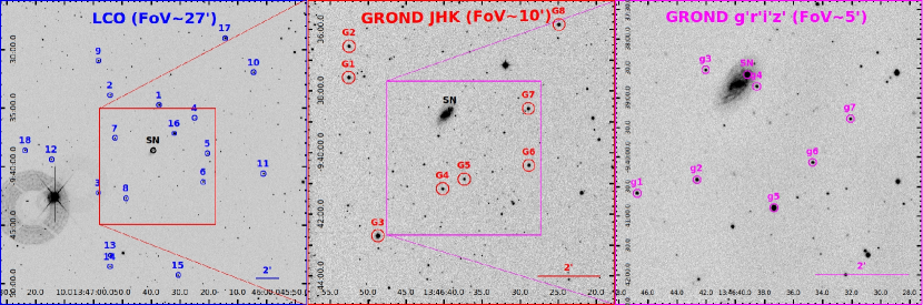
Figure 1: Left: LCO $V$-band image from 2019-06-30 showing the location of SN 2018evt. Local photometric reference stars are marked with blue circles. The red square outlines the GROND $JHK$ field of view (FoV) shown in the middle panel. Middle: GROND $J$-band image obtained on 2019-01-10 indicating the location of SN 2018evt. Local photometric reference stars used for the $JHK$ bands are marked with red circles and labeled with prefix “G”. The magenta square shows the size of the GROND $g^{\prime}r^{\prime}i^{\prime}z^{\prime}$-band FoV. Right: GROND $g^{\prime}$-band image of SN 2018evt obtained on 2019-01-10. Local photometric reference stars used for the $g^{\prime}r^{\prime}i^{\prime}z$ bands are marked with magenta circles and labeled with prefix “g”. The FoV and the angular scale (2′) are also marked in each panel. North is up, east is to the left.

2 Observations and Data Reduction

SN 2018evt (ASASSN-18ro) was discovered by the All-Sky Automated Survey for Supernovae (ASAS-SN; Shappee et al., 2014) on 2018-08-11 (UT dates are used throughout this paper; MJD 58341.005) at $V\approx 16.5$ mag (absolute magnitude $M_{V}\approx-18.7$ mag; Nicholls & Dong, 2018). Follow-up spectroscopy was obtained by the extended Public ESO Spectroscopic Survey for Transient Objects (ePESSTO; Smartt et al., 2015) with the New Technology Telescope (NTT) + ESO Faint Object Spectrograph and Camera 2 (EFOSC2; Buzzoni et al., 1984) on 2018-08-12 23:59 (MJD 58343.000; Stein et al., 2018). Cross-correlation with a library of SN spectra using the “Supernova Identification code” (SNID; Blondin & Tonry, 2007) suggests that the spectrum matches SN 1991T-like templates at $-9$ days relative to the $B$-band maximum. Because of the lack of early-time data, we adopt a peak-light epoch at MJD 58352 based on the best match from SNID but do not attempt to estimate the uncertainty. All phases are given relative to the roughly estimated $B$-band peak luminosity at MJD 58352 or 2018-08-22 (see Sec. 3) throughout the paper.

Astrometric measurements on the images obtained by the Sinistro cameras of the Las Cumbres Observatory (LCO) global network of 1 m telescopes (see Sec. 2.1.1) has been derived by using Astrometry.net (Lang et al., 2010). The world coordinate system (WCS) was solved for each frame and calibrated to the GAIA DR2 catalog (Gaia Collaboration et al., 2016, 2018). We chose a total of six exposures obtained by LCO in $g^{\prime}r^{\prime}i^{\prime}$ under very good conditions on 2019-05-09 (MJD 58612) to calculate the centroids of the SN and the host nucleus. We selected $\sim 100$ bright (signal-to-noise ratio [SNR] $>50$), isolated field stars within a $20\arcmin\times 20\arcmin$ box around the SN, cross-correlated their coordinates against the GAIA DR2 catalog, and deduced a median offset of $\rm\alpha^{LCO}-\alpha^{GAIA}=-0\aas@@fstack{\prime\prime}{110}\pm 0\aas@@fstack{\prime\prime}{164}$ and $\rm\delta^{LCO}-\delta^{GAIA}=0\aas@@fstack{\prime\prime}{103}\pm 0\aas@@fstack{\prime\prime}{125}$.

Adopting the median value of the measurements obtained on the six frames and correcting for the offset between the LCO images and the GAIA DR2 catalog, we estimate the position of SN 2018evt as $\rm(\alpha,\delta)_{SN}=(13^{h}46^{m}39\aas@@fstack{\prime\prime}{181}\pm 0\aas@@fstack{\prime\prime}{003}\pm 0\aas@@fstack{\prime\prime}{164},\ -09^{\circ}38^{\prime}36\aas@@fstack{\prime\prime}{042}\pm 0\aas@@fstack{\prime\prime}{040}\pm 0\aas@@fstack{\prime\prime}{125}$). The coordinates of the nucleus of the host spiral galaxy MCG-01-35-011 are $\rm(\alpha,\delta)_{Host}=(13^{h}46^{m}39\aas@@fstack{\prime\prime}{779}\pm 0\aas@@fstack{\prime\prime}{004}\pm 0\aas@@fstack{\prime\prime}{164},\ -09^{\circ}38^{\prime}45\aas@@fstack{\prime\prime}{641}\pm 0\aas@@fstack{\prime\prime}{070}\pm 0\aas@@fstack{\prime\prime}{125})$; see Fig. 1. For each quantity, the first and the second uncertainties represent the errors due to filter-to-filter differences and the 1$\sigma$ deviation of the coordinate differences among the stars used in the cross-calibration, respectively.

The heliocentric radial velocity of the host galaxy amounts to $7600\pm 40$ km s^-1 (da Costa et al., 1998). From the peak wavelength of the well-resolved narrow H$\alpha$ P Cygni profile in the flux spectrum obtained with a higher spectral resolution, we deduce the redshift of SN 2018evt to be $z=0.02523\pm 0.00015$ (for more details, see Sec. 4.2). This value is consistent with the reported redshift of the host galaxy; it is used throughout the paper. We interpret the radial velocity as exclusively due to redshift and adopt a Hubble constant of H${}_{0}=73.24\pm 1.74$ km s^-1 Mpc^-1(Riess et al., 2016). We derive a distance for the host of $103.3\pm 2.5$ Mpc. We measure the angular separation between SN 2018evt and the nucleus of its host as 13$\aas@@fstack{\prime\prime}$0, corresponding to a sky-projected separation of $6.5\pm 0.2$ kpc.

2.1 Optical and NIR Photometry

2.1.1 Las Cumbres Optical Photometry

Extensive $Bg^{\prime}Vr^{\prime}i^{\prime}$ photometry was acquired with the Sinistro cameras of the LCO network of 1 m telescopes. The data were taken as part of the Global Supernova Project. The pixel size is $0\aas@@fstack{\prime\prime}{389}$ pixel^-1, and most of the measured full widths at half maximum (FWHMs) of the point-spread function (PSF) fall within the range of $1\aas@@fstack{\prime\prime}{4}$ to $2\aas@@fstack{\prime\prime}{5}$. The images were preprocessed, including bias subtraction and flat-field correction, with the BANZAI automatic pipeline (McCully et al., 2018). Figure 1 (left panel) shows the field around SN 2018evt. For each frame, the PSF was determined from bright, isolated field stars and matched to the SN and local comparison stars. The PSF model fitting radius was chosen as the FWHM. Owing to the lack of template images obtained by LCO before the SN exploded, we estimate the galaxy contribution by fitting a median pixel value of an annulus around the SN with an inner radius of 4$\aas@@fstack{\prime\prime}$0 and an outer radius of 5$\aas@@fstack{\prime\prime}$5. The background was determined and subtracted iteratively during the fitting of the PSF using the ALLSTAR task under the IRAF DAOPHOT package (Stetson, 1987). The choice of the inner radius is justified by the fact that the residuals measured from the PSF-subtracted field stars were consistent with the noise beyond $\sim 1.5\times$ FWHM. The small inner and outer radii and the iteration procedure provide a realistic estimate of the local background of the SN. Employing magnitudes of 15 local comparison stars from the AAVSO Photometric All Sky Survey (APASS) DR9 Catalogue (Henden et al., 2016), we calibrated the instrumental $BV$ and $g^{\prime}r^{\prime}i^{\prime}$ magnitudes of SN 2018evt in the Johnson $BV$ system (Johnson, 1966) in Vega magnitudes and in the SDSS photometric system (Fukugita et al., 1996) in AB magnitudes (Oke & Gunn, 1983), respectively. The final $Bg^{\prime}Vr^{\prime}i^{\prime}$-band calibrations were derived from the median of the difference between catalogue and instrumental magnitudes. The $Bg^{\prime}Vr^{\prime}i^{\prime}$ comparison stars are identified in the left panel of Figure 1. We list the photometry of SN 2018evt in Table 7.

2.1.2 GROND Optical and NIR Photometry 

Simultaneous 7-band photometry in $g^{\prime}r^{\prime}i^{\prime}z^{\prime}JHK$ was obtained with the Gamma-Ray burst Optical/Near-infrared Detector (GROND; Greiner et al., 2008) mounted on the 2.2 m MPG/ESO telescope at the La Silla Observatory (Chile). The plate scales of the GROND optical ($g^{\prime}r^{\prime}i^{\prime}z$) and NIR ($JHK$) images are $0\aas@@fstack{\prime\prime}{389}$ pixel^-1 and $0\aas@@fstack{\prime\prime}{60}$ pixel^-1, respectively. In the NIR, the field of view (FoV) of $10^{\prime}\times 10^{\prime}$ is imaged onto a $1024\times 1024$ pixeo Rockwell HAWAII-1 array (pixel size 18.5 $\mu$m, plate scale $0\aas@@fstack{\prime\prime}{60}$ pixel^-1). The GROND pipeline resamples the NIR frame to 2k $\times$ 2k, yielding a pixel scale of $0\aas@@fstack{\prime\prime}{30}$ in the reduced images. The measured FWHM of the PSF from the GROND images ranges from $0\aas@@fstack{\prime\prime}{8}$ to $1\aas@@fstack{\prime\prime}{9}$. The median value of the measured FWHM during the entire observing sequence for different bandpasses is $1\aas@@fstack{\prime\prime}{2}$ with small variations (i.e., $1\aas@@fstack{\prime\prime}{1}$ for the $g^{\prime}$ band and $1\aas@@fstack{\prime\prime}{3}$ for the $H$ band). The fluxes of the SN and local reference stars were determined following a similar PSF-fitting procedure as for the LCO photometry. The inner and outer radii of the annulus were chosen to be 3$\aas@@fstack{\prime\prime}$0 and 4$\aas@@fstack{\prime\prime}$5, respectively. No images of the SN 2018evt field were obtained by GROND before the SN exploded, so template subtraction could not be performed.

The GROND $g^{\prime}r^{\prime}i^{\prime}z^{\prime}$ photometry was calibrated relative to PanSTARRS1 (Chambers et al., 2016) field stars in the AB system. The different sets of photometric standards for the GROND and LCO observations are mandated by the different FoVs: 5′ for GROND optical, 10′ for GROND NIR ($JHK$), and 27′ for the Sinistros. NIR magnitudes ($JHK$) were derived with respect to Two Micron All Sky Survey (2MASS; Cutri et al., 2003) field stars in the Vega system. The final calibration of the GROND photometry is based on the median difference between catalogue and instrumental magnitudes of seven and eight field stars in the $g^{\prime}r^{\prime}i^{\prime}z^{\prime}$ and $JHK$ bands, respectively. These stars are identified by the purple and red circles in the right panel of Figure 1. The GROND photometry is tabulated in Table 8.

The resulting LCO $g^{\prime}$ and $r^{\prime}$ light curves display offsets from the corresponding GROND photometry (Fig. 2). The difference between the two light curves may be caused by the different calibration catalogues. Querying the APASS and PanSTARRS1 catalogues centred on SN 2018evt with a box size of the LCO FoV, we found from more than 100 stars in common to both catalogues the median of the differences in magnitude and associated 1$\sigma$ ranges of $g_{\rm APASS}-g_{\rm Panstarrs1}\approx 0.05\pm 0.06$ mag and $r_{\rm APASS}-r_{\rm Panstarrs1}\approx-0.02\pm 0.06$ mag.

2.2 Optical Spectroscopy

A journal of the spectroscopic observations of SN 2018evt can be found in Table 1. In addition to the early NTT classification spectrum (day $-9$), the late-time spectral sequence of SN 2018evt spans days 129 to 365. Apart from the EFOSC flux spectra described in Section 2, the spectral database consists of LCO optical spectra taken with the FLOYDS spectrographs mounted on the 2 m Faulkes Telescopes North and South at Haleakala, USA (FTN) and Siding Spring, Australia (FTS), through the Global Supernova Project (Brown et al., 2013). A 2$\arcsec$ slit was placed on the target at the parallactic angle (Filippenko, 1982). One-dimensional spectra were extracted, reduced, and calibrated following standard procedures using the FLOYDS pipeline (Valenti et al., 2014). The $Bg^{\prime}Vr^{\prime}i^{\prime}$ light curves and FLOYDS/LCO spectra were obtained as part of the Global Supernova Project. All photometry and spectroscopy will become available via WISeREP (Yaron & Gal-Yam, 2012).

2.3 VLT Imaging Polarimetry

SN 2018evt was observed with FORS at the Cassegrain focus of UT1 at the VLT in imaging polarimetric mode (IPOL) as part of the Type Ia SN imaging polarimetry survey (Prog. ID 0102.D-0163(A), PI Cikota). The observations were obtained through the standard b_HIGH (on 2019-01-09/day 140) and v_HIGH (on 2019-01-10/day 141) FORS2 filters, with half-wave retarder plate angles of $\theta=0^{\circ}$, $22.5^{\circ}$, $45^{\circ}$, and $67.5^{\circ}$ at each epoch.

All frames were bias subtracted using dedicated bias frames, and we removed particle events using LACosmic (van Dokkum, 2001). Aperture photometry with a radius of 2 times the FWHM [$2\times 0\aas@@fstack{\prime\prime}{44}$ ($2\times 3.5$ pixels) in the b_HIGH images and $2\times 0\aas@@fstack{\prime\prime}{45}$ ($2\times 3.6$ pixels) in the v_HIGH images] was performed in the ordinary and extraordinary beams using the DAOPHOT.PHOT package (Stetson, 1987). The linear polarization and the polarization angle were derived following the FORS2 manual (Anderson, 2018). The Stokes $Q$ and $U$ values and the polarization angle were corrected for the chromatism of the half-wave plate, and the polarization was debiased following Wang et al. (1997). In order to study the intrinsic geometry of the SN, the interstellar polarization estimated in Section 5.1 was subtracted from both the imaging and the spectropolarimetry.

On 2019-01-10/day 141, we measured a high linear polarization of $\sim 1.4$% in the $B$ and $V$ bands. Since the high polarization level of SN 2018evt suggested significant contributions intrinsic to the SN, we requested Director’s Discretionary Time observations with FORS2 on the VLT to obtain multi-epoch spectropolarimetry (Prog. ID 2102.D-5031, PI Wang) for the geometric characterisation of the SN ejecta, the massive CSM, and the ejecta-CSM interaction region.

2.4 VLT Spectropolarimetry

Spectropolarimetry of SN 2018evt was conducted with the FOcal Reducer and low-dispersion Spectrograph 2 (FORS2; Appenzeller et al., 1998) on Unit Telescope 1 (UT1, Antu) of the ESO Very Large Telescope (VLT). Observations were carried out in the Polarimetric Multi-Object Spectroscopy (PMOS) mode at four epochs: days 172/2019-02-10, 195/2019-03-05, 198/2019-03-08, and 219/2019-03-29. For each epoch, a flux standard star was observed at half-wave plate angle $0^{\circ}$. Grism 300V and a 1$\arcsec$ slit were used at epochs 1, 2, and 4. According to the VLT FORS2 user manual (Anderson, 2018), this configuration provides a spectral resolving power of $R\approx 440$ (or 13 Å FWHM) at a central wavelength of 5849 Å. VLT observations at epoch 3 were obtained with grism 1200R and a $1\arcsec$ slit, providing a spectral resolving power $R\approx 2140$ (or 3 Å FWHM) at a central wavelength of 6530 Å). A log of the VLT spectropolarimety is presented in Table 2.

Table 1: Log of spectroscopic observations of SN 2018evt.

UT Time	MJD	Phasea	Range	Resolving Power	Exp. Time	Instrument/Telescope
(yy-mm-dd hh:mm)		(days)	(Å)	(blue/red)	(s)
18-08-12 23:59	58343.00	$-$9.0	3600$-$9000	$\sim$18 Åb	300	EFOSC2+gm13/NTT 3.6 m
18-12-24 15:16	58476.64	124.6	3400$-$9800	619/500	1800	FLOYDS/LCO 2.0 m FTN
19-01-01 16:45	58484.70	132.7	3400$-$9800	497/398	1600	FLOYDS/LCO 2.0 m FTS
19-01-11 13:56	58494.58	142.6	3400$-$9800	413/513	1600	FLOYDS/LCO 2.0 m FTN
19-01-21 15:15	58504.64	152.6	3400$-$9800	627/498	1600	FLOYDS/LCO 2.0 m FTN
19-02-10 06:37	58524.28	172.3	4100$-$9100	440	480$\times$4	FORS2/PMOS+300V/VLT 8.2 m
19-03-04 10:21	58546.43	194.4	3400$-$9800	626/510	1800	FLOYDS/LCO 2.0 m FTN
19-03-05 06:00	58547.25	195.3	3400$-$9100	440	640$\times$4	FORS2/PMOS+300V/VLT 8.2 m
19-03-08 05:23	58550.22	198.2	5700$-$7100	2140	570$\times$4	FORS2/PMOS+1200R/VLT 8.2 m
19-03-17 11:39	58559.48	207.5	3400$-$9000	639/502	1800	FLOYDS/LCO 2.0 m FTN
19-03-29 04:53	58571.20	219.2	3400$-$9100	440	570$\times$4	FORS2/PMOS+300V/VLT 8.2 m
19-03-30 11:45	58572.49	220.5	3400$-$9800	622/504	1800	FLOYDS/LCO 2.0 m FTN
19-04-23 15:47	58596.66	244.7	3400$-$9800	469/396	2700	FLOYDS/LCO 2.0 m FTS
19-05-11 09:19	58614.39	262.4	3400$-$9800	382/540	2700	FLOYDS/LCO 2.0 m FTN
19-06-09 08:48	58643.37	291.4	3400$-$9800	604/542	2700	FLOYDS/LCO 2.0 m FTN
19-07-15 06:06	58679.25	327.3	3400$-$9800	641/553	3600	FLOYDS/LCO 2.0 m FTN
19-08-22 08:54	58717.37	365.4	3700$-$9800	641/553	3600	FLOYDS/LCO 2.0 m FTN

^aDays after $B$-band maximum on MJD 58352 / 2018 Aug. 22.
^bResolution in Å (FWHM).

Table 2: Log of spectropolarimetic observations.

Epoch	Object	Date	Phasea	Exposure	Grism / Resol. Power	Mean
		(UT)	(day)	(s)		Airmass
1	SN 2018evt	2019-02-10	172.3	$4\times 480$	300V/440	1.23
	CD-32d9927b	2019-02-10	–	$1\times 10$	300V/440	1.16
2	SN 2018evt	2019-03-05	195.3	$4\times 640$	300V/440	1.09
	L595-22b	2019-03-05	–	$1\times 60$	300V/440	1.01
3	SN 2018evt	2019-03-08	198.2	$4\times 570$	1200R/2140	1.14
	CD-32d9927b	2019-03-08	–	$4\times 20$	1200R/2140	1.08
4	SN 2018evt	2019-03-29	219.2	$4\times 570$	300V/440	1.06
	CD-32d9927b	2019-03-29	–	$1\times 20$	300V/440	1.03

^aRelative to the estimated peak on MJD 58352.
^bFlux standard, observed at a half-wave plate angle of $0^{\circ}$.

The high spectral resolution configuration in epoch 3 enabled us to measure more details of the spectropolarimetric properties across the H$\alpha$ profile, which mostly fall in the spectral range 5750–7310 Å. Only at epochs 1 and 3 was the GG435 filter used, which has a cutoff at $\sim 4350$ Å and serves to prevent shorter-wavelength second-order contamination. The effect of second-order contamination on spectropolarimetry is mostly negligible unless the source is very blue (see the Appendix of Patat et al., 2010). The absence of the GG435 filter at epochs 2 and 4 is deliberate to extend the blue coverage as the SN aged, and any contamination by second-order light was considered negligible in extracting the true polarization signal. The slit position angle, $\chi$, was aligned with the north celestial meridian (i.e., $\chi=0$). Since all observations were conducted at small airmass ($\lesssim 1.2$), the loss of blue light can be well compensated by the linear atmospheric dispersion compensator (LADC; Avila et al., 1997). Therefore, we consider any effect on the spectral energy distribution (SED) caused by the misalignment between $\chi$ and the parallactic angle to be negligible.

For each epoch of observation, four exposures were carried out at retarder-plate angles of $0^{\circ}$, $22.5^{\circ}$, $45^{\circ}$, and $67.5^{\circ}$. The data were bias subtracted and flat-field corrected. Extraction of the ordinary (o) and extraordinary (e) beams was achieved following standard procedures within IRAF. Wavelength calibration was carried out separately for the o-ray and e-ray in each individual exposure (all four retarder-plate angles) using He-Ne-Ar arc-lamp exposures. A typical root-mean-square (RMS) accuracy of $\sim 0.25$ Å was achieved. Calculation of the Stokes parameters, as well as the determination of the bias-corrected polarization and associated errors, were performed with our own routines, following the recipes of Patat & Romaniello (2006) and Maund et al. (2007). A wavelength-dependent instrumental polarization in FORS2 ($\lesssim 0.1$%) was further corrected based on the quantification by Cikota et al. (2017). More detailed descriptions of the reduction of FORS spectropolarimetry can be found in a recent FORS2 Spectropolarimetry Cookbook and Reflex Tutorial, as well as in Cikota et al. (2017) and Appendix A of Yang et al. (2020).

We write the observed polarization degree and position angle ($p_{\rm obs}$, PA_obs) and the true values after bias correction ($p$, PA) in terms of the intensity ($I$)-normalised Stokes parameters ($Q$, $U$) as

$$p_{\rm obs}=\sqrt{Q^{2}+U^{2}},\ p=(p_{\rm obs}-\sigma_{p}^{2}/p_{\rm obs})\times h(p_{\rm obs}-\sigma_{p});$$ (1)

$$PA_{\rm obs}=\frac{1}{2}{\rm arctan}\bigg{(}\frac{U}{Q}\bigg{)},\ {\rm\ and\ }PA=PA_{\rm obs}.$$

Correction of the polarization bias followed the equations of Simmons & Stewart (1985) and Wang et al. (1997), where $\sigma_{p}$ and $h$ give the $1\sigma$ uncertainty in $p_{\rm obs}$ and the Heaviside step function, respectively.

3 Light Curves of SN 2018evt

In Figure 2, we show the $Bg^{\prime}Vr^{\prime}i^{\prime}$-band light curves without correction for interstellar extinction. The $Bg^{\prime}Vr^{\prime}i^{\prime}$ light curves were sampled during the period $t\approx$ 124 to 368 days. We list the calibrated LCO $Bg^{\prime}Vr^{\prime}i^{\prime}$ photometry in Table 7; the magnitudes are not corrected for extinction in the host galaxy or the Milky Way. We also present the Zwicky Transit Facility (ZTF; Bellm et al., 2019) $g$ and $r$ light curves of SN 2018evt obtained with the forced-PSF photometry based on the pipeline developed by Yao et al. (2019). The results are shown in Table 9.

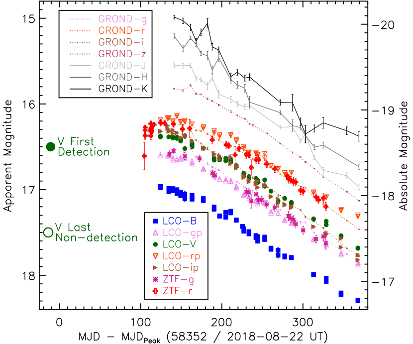
Figure 2: The optical and NIR light curves of SN 2018evt.

3.1 Interstellar Extinction Correction

The Galactic reddening along the line of sight to SN 2018evt was estimated as $E(B-V)^{\rm MW}_{\rm 18evt}=0.051$ mag by means of the NASA/IPAC NED Galactic Extinction Calculator and the extinction map by Schlafly & Finkbeiner (2011). Although an empirical relation between dust extinction and strength of the Na I D $\lambda\lambda 5890$, 5896 absorption doublet has been proposed (Munari & Zwitter, 1997) and is widely applied in extinction estimations, the validity of the method has been questioned for use with low-resolution spectra (Poznanski et al., 2011). Since all spectroscopic observations discussed in this study were carried out in the low- and medium-resolution regime, we do not consider extinction corrections based on interstellar Na I D lines. In the epoch-3 VLT spectrum ($R\approx 2140$), the spectral resolution is $\sim 2.8$ Å at Na I D. Limited by the insufficiently high spectral resolution, we calculate upper limits of the equivalent widths (EWs) of the two features as 0.47 Å and 0.37 Å for the Milky Way, and 0.66 Å and 0.50 Å for the host galaxy. Adopting an empirical relation between Na I D line width and dust reddening (Poznanski et al., 2012), we place upper limits on the extinction from the Milky Way and the host galaxy of $E(B-V)_{\rm MW}^{\rm Na~{}I~{}D}\textless 0.14\pm 0.02$ and $E(B-V)_{\rm Host}^{\rm Na~{}I~{}D}\textless 0.32\pm 0.05$, respectively. The intrinsically depolarized narrow H$\alpha$ emission line as measured from the high-resolution polarization spectrum at epoch 3 also suggests a low level of host reddening. See Section 5.1 for more details.

3.2 Pseudobolometric Light Curves

To better quantify the luminosity evolution of SN 2018evt, we computed its pseudobolometric luminosity over a range of wavelengths ($\sim 3870$–23,200 Å using the LCO $Bg^{\prime}Vr^{\prime}i^{\prime}$ optical and GROND $zJHK$ NIR photometry. The steps of the procedure are detailed in Appendix A.

The optical and optical-NIR pseudobolometric light curves of SN 2018evt are plotted in Figure 3. For comparison, we also applied the same procedure to the $Bg^{\prime}Vr^{\prime}i^{\prime}zJHK$ photometry of SN 2012ca (Inserra et al., 2016). We adopt a distance modulus of $39.454\pm 0.014$ mag for SN 2012ca (Shappee & Stanek, 2011), which is the same as the distance applied in the bolometric luminosity calculation conducted by Inserra et al. (2016). The calculated pseudobolometric light curve of SN 2012ca is also shown in Figure 3. The integration of the SN 2012ca SED was performed over the same wavelength ranges as for SN 2018evt. The middle panel presents the ratio of the optical (Opt, 3870–9000 Å) to optical–NIR (Opt–NIR, 3870–23,200 Å) flux. The Opt/Opt–NIR flux ratio ($F_{\rm Opt}/F_{\rm Opt-NIR}$) of SN 2018evt is lower than that of SN 2012ca.

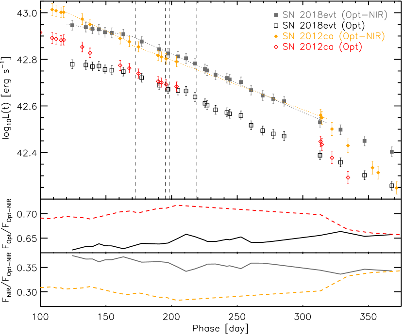
Figure 3: Pseudobolometric light curves of SNe 2018evt and 2012ca in the upper panel. Open black squares represent the bolometric luminosity integrated over the optical wavelength range (3870–9000 Å) while filled grey squares present the total bolometric luminosity within the optical-NIR wavelength range (3870–23,200 Å). Open red and filled orange diamonds give these quantities calculated for SN 2012ca. The dotted grey line segments fit the optical-NIR bolometric decline rate of SN 2018evt from days 120 to 170 and from days 170 to 320, respectively. The dotted orange line segments present the similar fit to SN 2012ca. Vertical dashed lines mark the times of spectropolarimetric observations of SN 2018evt. The middle and lower panels present the fractions of the optical and the NIR (9000–23,200 Å) fluxes of the total bolometric flux for SNe 2018evt (solid line) and 2012ca (dashed line), respectively.

We tabulate the optical and optical–NIR pseudobolometric luminosities of SN 2018evt in Table 10. As a sanity check, a comparison was carried out between the pseudobolometric luminosity of SN 2012ca derived by Inserra et al. (2016) and our calculation. We found that SN 2012ca has a maximum pseudobolometric luminosity of $L_{\rm Opt}=(1.37\pm 0.07)\times 10^{43}$ erg s^-1 and a peak optical–NIR luminosity of $L_{\rm Opt-NIR}=(1.84\pm 0.10)\times 10^{43}$ erg s^-1. These values are consistent with those published by Inserra et al. (2016): $L_{\rm pseudobol}\approx 1.29\times 10^{43}$ erg s^-1 and $L_{\rm bol}\approx 1.90\times 10^{43}$ erg s^-1, respectively. Since no data were obtained from days $\sim-10$ to 120, we do not attempt to estimate the peak bolometric luminosity of SN 2018evt. As presented in Figure 3, we suggest that the luminosity of SN 2018evt is similar to that of SN 2012ca at similar phases.

About 170 days after the estimated time of peak luminosity, the decline rate of the bolometric luminosity of SN 2018evt changed from $-0.111\pm 0.010$ to $-0.226\pm 0.002$ dex (100 days)^-1 as shown in Figure 3. Between days 170 and 320, SN 2018evt exhibited a similar decline rate as SN 2012ca. The steeper decline at later phases (days $\sim 300$–400) observed in all three events presented by Inserra et al. (2016) with data after a year from the peak (i.e., SNe 1997cy, 1999E, and 2012ca) was not followed by SN 2018evt. Conversely, none of these three SNe showed an earlier break at a similar phase as SN 2018evt. The logarithmic luminosity decline rates of SNe 2018evt and 2012ca over different phases are listed in Table 3.

Since a break in the bolometric light curve was found around day 170 (Sec. 3.2), before the epoch of the optical SED template used in the above calculations, we also performed the same analysis using the FLOYDS/LCO spectrum on day 125 as the template SED of SN 2018evt in the optical. This spectrum was obtained before the bolometric luminosity break. It has a similar profile to all the late-time spectra, but with relatively weaker line-emission features. The pseudobolometric flux calculated from the day-125 spectrum is overall $\sim 1.5$% lower than that from the day-219 spectrum. This systematic difference between the different SED converts to 0.007 in log $L$ or $\sim 1/3$ of the total uncertainty of the pseudobolometric luminosity. Therefore, we suggest that the early break in the bolometric flux has no significant effect on the late-time spectral evolution.

Table 3: Luminosity decline rates of SNe 2018evt and 2012ca.

SN	Phasea	Decline rate, log $L$/time
	[days]	[log (erg s-1)/100 d]
2018evt	120$-$170	$-$0.105$\pm$0.009
	170$-$320	$-$0.250$\pm$0.004
2012ca	120$-$170	$-$0.266$\pm$0.008
	170$-$320	$-$0.213$\pm$0.002
	120$-$320	$-$0.229$\pm$0.005
	380$-$560	$-$0.460$\pm$0.011

^aRelative to the estimated peak at MJD 58352.

4 Spectroscopy

Figure 4 presents our spectral sequence of SN 2018evt. In addition to the initial classification spectrum obtained with EFOSC2 on the NTT, the dataset consists of 16 further optical spectra spanning the interval from approximately days 125 to 365. All wavelengths were corrected for the redshift of the host galaxy.

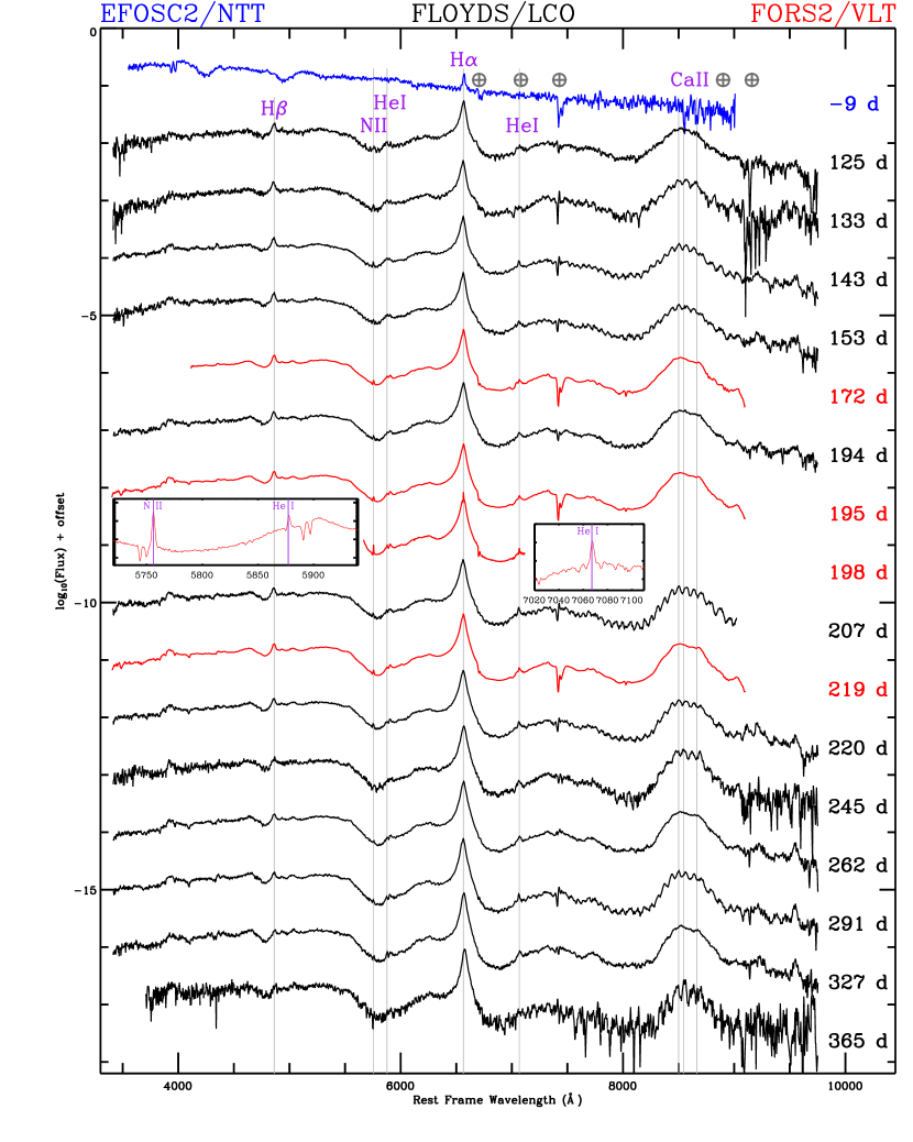
Figure 4: Spectral time series of SN 2018evt observed by NTT, LCO, and VLT (solid curves, phases are marked on the right; colours distinguish the spectrographs as shown at the top). Several prominent spectral lines are labeled, and some telluric lines are marked by crossed circles. The semi-regular fluctuations above $\sim 8000$ Å in some of the spectra are caused by fringing in the detectors; at still longer wavelengths, atmospheric water-vapor absorption sets in.

4.1 Evolution of the H$\alpha$ and H$\beta$ Lines

The prominent Balmer emission features in the late-time spectra indicate that the spectral evolution of SN 2018evt is slow and resembles that of other known SN 1997cy-like events. It has been suggested that the H$\alpha$ region in these objects can be characterised by a pseudocontinuum plus multiple emission components (e.g., Hamuy et al., 2003; Deng et al., 2004; Kotak et al., 2004). We suggest that the late-time H$\alpha$ emission of SN 2018evt is satisfactorily described by a combination of a broad and an intermediate Gaussian component. The details of the fitting procedure is described in Appendix B.

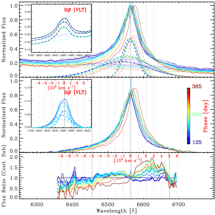
Figure 5: Temporal evolution of the H$\alpha$ profile of SN 2018evt. All spectra were corrected for Galactic extinction and are shown in the rest frame. The phases are colour coded as indicated by the vertical colour bar. In the upper panel, solid lines present the peak-normalised spectra. Dotted straight lines, dot-dashed curves, and dashed curves represent the pseudocontinuum and Gaussian fits to the broad and the intermediate components, respectively. The middle panel displays the H$\alpha$ profiles after subtracting the pseudocontinuum. Upper and middle insets show similar diagrams for H$\beta$ in the high-SNR VLT observations, indicating that the H$\beta$ profile can also be described with two Gaussian components like those of H$\alpha$. The H$\alpha$ profiles in the middle panel but divided by that of the first epoch on day 125 are plotted in the bottom panel. Wavelengths corresponding to different velocities relative to the H$\alpha$ peak in the rest frame are shown as vertical grey lines and labeled.

Figure 5 illustrates the evolution of the H$\alpha$ emission of SN 2018evt from days $\sim$125 to 365. The profile exhibits a prominent emission on an underlying quasi-continuum. The latter could be formed by the blending of relatively narrow lines of iron-group elements from fragmented cool shocked ejecta, mostly Fe ii lines (Chugai et al., 2004). In the upper panel of Figure 5, we present the H$\alpha$ profiles with the peak normalised to unity. Spectra after subtracting the pseudocontinuum are shown in the middle panel. To better expose the temporal evolution of the H$\alpha$ profile, we divided all late-phase spectra by our first late-time spectrum taken at day 125. Flux ratios were calculated from the normalised, pseudocontinuum-subtracted spectra and are shown in the bottom panel of Figure 5.

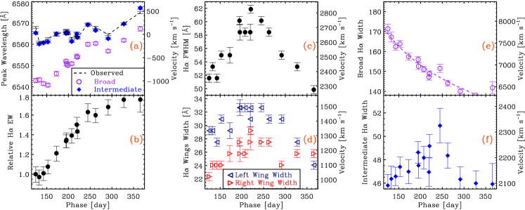
Figure 6: Evolution of H$\alpha$ emission parameters. Panel (a) shows the measured wavelength of the peak, together with the fitted central wavelengths of the broad and intermediate components, as a function of phase. Panel (b) depicts the ratio between the time series of the H$\alpha$ equivalent width and that measured at day $+$125 when the first late-time spectrum of SN 2018evt was obtained. Panels (c) and (d) present the time evolution of the FWHM, and the widths measured in the blue and the red emission wings only (all three in velocity units). Panels (e) and (f) give the width of the broad and the intermediate H$\alpha$ components, respectively. Except for panel (b), the corresponding velocities can be read off the right-hand ordinates.

In Figure 6, we plot the temporal evolution of the H$\alpha$ profile as encoded in several of its properties. We show the central wavelengths of the observed peak, the fitted broad and intermediate components (Fig. 6a), the total FWHM (Fig. 6c), and the widths of the blue and the red wing alone (Fig. 6d). The absolute value of the pseudo-equivalent width (pseudo-EW; $W_{\lambda}$) of the H$\alpha$ emission in Figure 6b is defined as $W_{\lambda}=\int_{\lambda_{\rm blue}^{\rm H\alpha}}^{\lambda_{\rm red}^{\rm H\alpha}}\left|\frac{f_{c}(\lambda)-f(\lambda)}{f_{c}(\lambda)}\right|d\lambda$, where $f(\lambda)$ and $f_{c}(\lambda)$ denote the flux across the emission line and the underlying continuum (respectively) at wavelength $\lambda$. Figures 6e and 6f present the width of the broad and the intermediate H$\alpha$ components, respectively. The 1$\sigma$ uncertainty of $W_{\lambda}$ was derived by error propagation of the uncertainty in the pseudocontinuum fitting. The absolute value of the pseudo-EW of an emission line measures how large a (pseudo)continuum range would have to be integrated over in order to obtain the same energy flux as contained in the emission line. To quantify the temporal evolution of the width of the H$\alpha$ profile, we divided $W_{\lambda}$ computed for different phases by that calculated for the first late-time spectrum acquired at day $+$125 and presented the result in Figure 6b.

In Figure 6a, one can see that the peak wavelength of both the continuum-subtracted flux spectrum (the black dashed line labelled “Observed”) and the intermediate component (blue filled diamonds) were confined to a narrow range of $\sim\pm 200$ km s^-1 before day 300, and started to shift toward longer wavelengths afterward. By contrast, the central wavelength of the broad component drifted from $-1200$ km s^-1 to $\sim+100$ km s^-1 between days 125 and 365. In Figure 6c, the FWHM (in velocity units) of the H$\alpha$ profile shows a monotonic increase from $\sim 2350$ km s^-1 and reached a maximum of $\sim 2800$ km s^-1 at day $\sim 220$, and then decreased to $\sim 2300$ km s^-1 at day $\sim 365$. This general trend is also shared by the widths of the blue and the red wings characterised by the absolute value of $W_{\lambda}$ as presented in the bottom-right panel. In Figure 6d, the absolute value of the H$\alpha$ pseudo-EW increases continuously until day $\sim 240$ by as much as 80%.

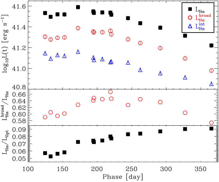
Figure 7: Temporal evolution of the H$\alpha$ luminosity and the contribution of its different components of SN 2018evt. The top panel compares the H$\alpha$ luminosity with the flux from the Gaussian-decomposed broad and intermediate components. The middle panel presents the flux ratios between the broad component and the H$\alpha$ luminosity. The bottom panel shows the ratio between the H$\alpha$ and the optical bolometric luminosities.

black H$\alpha$ luminosity of SN 2018evt from days 125 to 365 is shown in Figure 7. Flux contribution from the pseudocontinuum has been subtracted. The temporal evolution of the broad and the intermediate components based on the Gaussian decomposition, the ratio between the broad component and the H$\alpha$ luminosity, $\rm L_{H\alpha}^{broad}/L_{H\alpha}$, and the ratio between the H$\alpha$ and the optical luminosities, $\rm L_{H\alpha}/L_{opt}$ are also presented. From day 125, the H$\alpha$ and the flux of the broad component increase with time, while the flux of the intermediate component stays roughly constant. After reaching the peak at around days $\approx$170–220, both the broad and the intermediate components decrease monotonically. The ratio between the luminosity of the broad component and the H$\alpha$ profile, except for the first two epochs where it is more difficult to measure. The FWHM of the central Gaussian is rather constant, but it decreases in the last two spectra. The luminosities of the two components behave similarly, rising to a peak and then declining. SN 2018evt exhibits comparable strength of H$\alpha$ emission to SNe 1997cy (Turatto et al., 2000), 1999E (Hamuy et al., 2003), and 2002ic (Wang et al., 2004) at similar phases. The primary energy source of the broad H$\alpha$ is the interaction between the SN ejecta and the CSM, and its luminosity is proportional to the dissipation rate of the kinetic energy across the shock front (Kotak et al., 2004). The intermediate component is most likely arises from the preionized gas in the unshocked, optically thick CSM (Taddia et al., 2020). The origin of the different H$\alpha$ components will be discussed in Section 7.2.

4.2 The H$\alpha$ P Cygni Profile

VLT/FORS2 epoch-3 observations obtained with Grism 1200R provides a higher spectral resolving power ($R\approx 2140$) than the rest of the spectra presented in this work. The corresponding resolution element $\delta\lambda=\lambda/R\approx 3$ Å at the central wavelength of 6530 Å enables a detailed study of the narrow P Cygni core of the H$\alpha$ emission (rest-frame wavelength $\lambda_{0}^{\rm H\alpha}=6564.614$ Å) that is only revealed at this higher resolution. Therefore, a multiple-component Gaussian fitting process similar to that used with the lower-resolution spectra was applied to this P Cygni core. The pseudocontinuum was approximated by a low-order polynomial fitted to the spectrum between 5700 and 7300 Å with the H$\alpha$-dominated range 6300–6700 Å excluded. Apart from the broad and the intermediate components, two additional functions characterising the narrow absorption and the narrow emission components were included to fit the P Cygni core. The results are illustrated in the left panel of Figure 8.

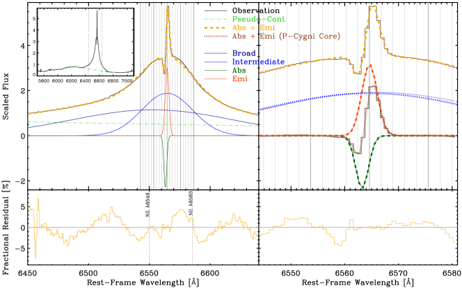
Figure 8: The H$\alpha$ profile of SN 2018evt in the VLT epoch-3 (day 198) spectrum fitted with multiple Gaussian functions. In the top-left panel, the observed spectrum (black histograms) is well approximated by the orange-dashed line, which consists of a pseudocontinuum (green dot-dashed line) and four Gaussian components, namely the broad (solid navy line), intermediate (solid blue line), and narrow (solid orange-red line) emission components and the narrow absorption (solid dark green line). The fractional residuals are provided in the bottom panel. The upper inset covers the full spectral range of the epoch-3 spectrum; the two vertical dashed lines mark the spectral range of the main panel. The top-right panel presents a three-component Gaussian fit to the spectrum near the H$\alpha$ core after subtracting the pseudocontinuum and the broad component. Blue-dotted, red-dashed, and green-dashed lines identify the intermediate and narrow emission components and the absorption, respectively. After further intermediate-component subtraction (grey histogram), the spectrum is well fitted by the narrow Gaussian absorption and emission components (brown dotted line). The fit to the core region is given by the orange dashed line. The fractional residuals are shown in the lower panel. Vertical grey lines are drawn at $\pm 1000$ km s^-1 relative to the H$\alpha$ narrow peak; 100 km s^-1 intervals are denoted by grey lines.

A more physical description of the H$\alpha$ profile would result from Monte Carlo simulations of selected structures of the electron-scattering zone (e.g., Huang & Chevalier, 2018). Moreover, the H$\alpha$ emission of CSM-interacting SNe may also be approximated with Lorentzian or exponent-modified Lorentzian profiles (Leonard et al., 2000; Smith et al., 2011). For example, the sum of a narrow Gaussian and a broad modified Lorentzian yielded a plausible fit in the case of the Type IIn SN 1998S (Shivvers et al., 2015). However, the physical interpretation of such a profile fitting is still not clear (see, e.g., Jerkstrand, 2017). There is no intuition for expecting that the H$\alpha$ emission can be represented by a superposition of a few simple functions. In our analysis, we also fitted the broad and the intermediate components with two Lorentzian functions as well as with a Gaussian plus a Lorentzian function, but found no significant improvement in the achieved quality. In view of the very limited knowledge of the CSM configuration and the arbitrarily defined pseudocontinuum, we descoped the decomposition and fitting of the H$\alpha$ profile to characterise the temporal evolution of the overall appearance of the feature.

In order to better separate the absorption and emission components of the P Cygni profile and determine the redshift and the wind velocity, a two-stage analysis was carried out in addition to a four-component Gaussian fit. In this latter process, the broad Gaussian component was removed along with the pseudocontinuum. Thereafter a three-component Gaussian fit to the spectrum near the H$\alpha$ core was performed over the wavelength interval 6544–6581 Å, roughly corresponding to a velocity range from $-950$ to $+750$ km s^-1. The results can be found in the right-hand panel of Figure 8. The narrow absorption and emission components together achieve an acceptable fit to the spectrum after further removal of the intermediate component. Assuming the narrow emission component has its peak at the rest-frame wavelength of the line, we measured a redshift $z=0.02523\pm 0.00015$ based on the three-component Gaussian fit over a narrow range near the H$\alpha$ emission core. This is consistent with the value deduced from the four-component Gaussian fitting ($z=0.02523\pm 0.00037$) and the redshift of the host galaxy reported by da Costa et al. (1998). The wind velocity inferred from the narrow, blueshifted absorption minimum is $v_{\rm wind}=63\pm 17$ km s^-1 (see Fig. 8). Note that the covariance between the fitted positions of the narrow emission and absorption components has been taken into account. We also conducted fits to the H$\alpha$ profile by adding additional Gaussian components and observed no improvement in the results.

4.3 Narrow Emission Lines

Several very narrow emission lines were identified in the late-time spectra of SN 2018evt. The most prominent feature is the [N ii] $\lambda$5755 forbidden emission. The line appears to have the same redshift as indicated by the narrow P Cygni H$\alpha$ component. Based on the VLT epoch-3 observations, we found that the FWHM of the line is consistent with the size of the spectral resolution element, $\Delta\lambda\approx 2.7$ Å. Therefore, the upper limit of the corresponding velocity is smaller than 140 km s^-1 within the N-rich matter, which is in agreement with the wind velocity inferred from the H$\alpha$ profile. We suggest that the N line forms in the CSM. The presence of the [N ii] $\lambda 5755$ line indicates that it originates from a cooler component of the CSM (i.e., less than a few $\times 10^{5}$ K; Salamanca et al., 2002).

The density of the CSM can be constrained by the intensity ratio of certain narrow lines. We measure the intensity ratio $I$([N ii $\lambda\lambda$6548, 6583])/$I$(N ii $\lambda 5755$) $\approx$0.18–0.28 from the VLT epoch-3 observations after subtracting either a pseudocontinuum or the multiple-component Gaussian fitting estimated from its ambient spectral region. The uncertainty of the intensity ratio depends mainly on the quality of the continuum removal and the wavelength ranges selected for the flux integration. Therefore, we calculated the intensity ratio for a series of wavelength bounds from $\pm 2$ to $\pm 4$ Å relative to the central wavelength. As the final value for $I$([N ii $\lambda\lambda$6548, 6583])/$I$(N ii $\lambda 5755$), we adopted a range of the values obtained with the aforementioned series of bounds. Following Equation 5.5 of Osterbrock (1989), for temperatures in the range $10^{4}<T<10^{7}$ K, the electron number density $n_{e}$ is between $\sim 2.9^{+0.8}_{-0.5}\times 10^{6}$ cm^-3 and $\sim 2.5^{+0.7}_{-0.5}\times 10^{7}$ cm^-3, with the lower bound of $n_{e}$ generally obtained at $T_{e}\approx 5\times 10^{4}$ K. The estimated high density in the CSM around SN 2018evt is broadly similar to those derived for SNe IIn; see, e.g., Salamanca et al. (2002) and Hoffman et al. (2008).

5 Polarimetry

In the next subsections, we present the VLT spectropolarimetry of SN 2018evt. First, we focus on the interstellar polarization. Second, we discuss the global intrinsic polarization properties of the SN and thereafter continue with the time evolution of the continuum polarization. Finally, we undertake a more detailed investigation of the polarization spectra across the most prominent H$\alpha$ emission at the late phases.

5.1 Interstellar Polarization

When light passes through the interstellar medium (ISM), it is polarized through dichroic absorption by nonspherical paramagnetic dust grains partially aligned by the large-scale magnetic field of the galaxy. The removal of this interstellar polarization (ISP) is essential for deriving the polarization vector intrinsic to the source. This step is challenging and requires a beacon shining through the ISM and tracing the ISP. The estimation of the ISP toward SNe usually relies on assumptions of certain parts of the intrinsic optical spectrum of the SN being unpolarized. Spectral signatures often considered unpolarized include (1) the late-time spectra of SNe ($\sim 40$ days after peak luminosity) when electron scattering in the substantially diluted ejecta is much reduced (e.g., Wang et al., 2001; Howell et al., 2001); (2) the blanketing by iron-group absorption features over certain wavelength ranges, e.g., $\sim 4800$–5600 Å (Howell et al., 2001; Chornock et al., 2006; Patat et al., 2009; Maund et al., 2010), where the electron-scattering opacity is dominated by line-blanketing opacity; and (3) the emission components of strong P Cygni profiles because the line emission is dominated by recombination photons (Wang et al., 2004, see also below). The assumption underlying all three cases is that any residual electron scattering does not contribute significantly to the total flux.

The narrow H$\alpha$ emission feature in the late-time spectra of SN 1997cy-like events is produced by the recombination of H in the nearly stationary CSM. Since the mechanism by which a proton captures an electron is distinct from the process causing a net polarization due to incomplete cancellation of electric vectors in the photosphere, H recombination lines are intrinsically unpolarized in the absence of strong magnetic fields. By contrast, the broad wings of the H$\alpha$ emission indicate the presence of fast-moving electrons in the CSM gas that is optically thick in H$\alpha$. Accordingly, following an approach similar to that of Wang et al. (2004), we adopt the value of the polarization at the narrow H$\alpha$ peak for our estimate of the ISP, which gives $p_{\rm ISP}=0.14\pm 0.08$%. The method is detailed in Appendix C.

An empirical rule for the dichroic extinction-induced ISP by Milky Way-like dust grains derived from observations of supposedly intrinsically unpolarized Galactic stars stipulates that $p_{\rm ISP}<9\%\times E(B-V)$ (Serkowski et al., 1975). For a standard Galactic $R_{V}=3.1$ extinction law (Cardelli et al., 1989), the upper limit on the ISP derived from the Milky Way reddening only, $E(B-V)=0.051$ mag, yields $p_{\rm ISP}<0.46$%. Accordingly, our ISP estimate passes this sanity check even in the case of vanishing extinction in the host galaxy. Therefore, we subtracted the above deduced $q_{\rm ISP}$ and $u_{\rm ISP}$ from all Stokes $Q$ and $U$ measurements in our VLT observations. The low line-of-sight polarization level of $\sim 0.14$% also suggests a low level of host reddening. Because of the relatively low ISP suggested by the low extinction toward SN 2018evt, we adopted a wavelength-independent ISP correction.

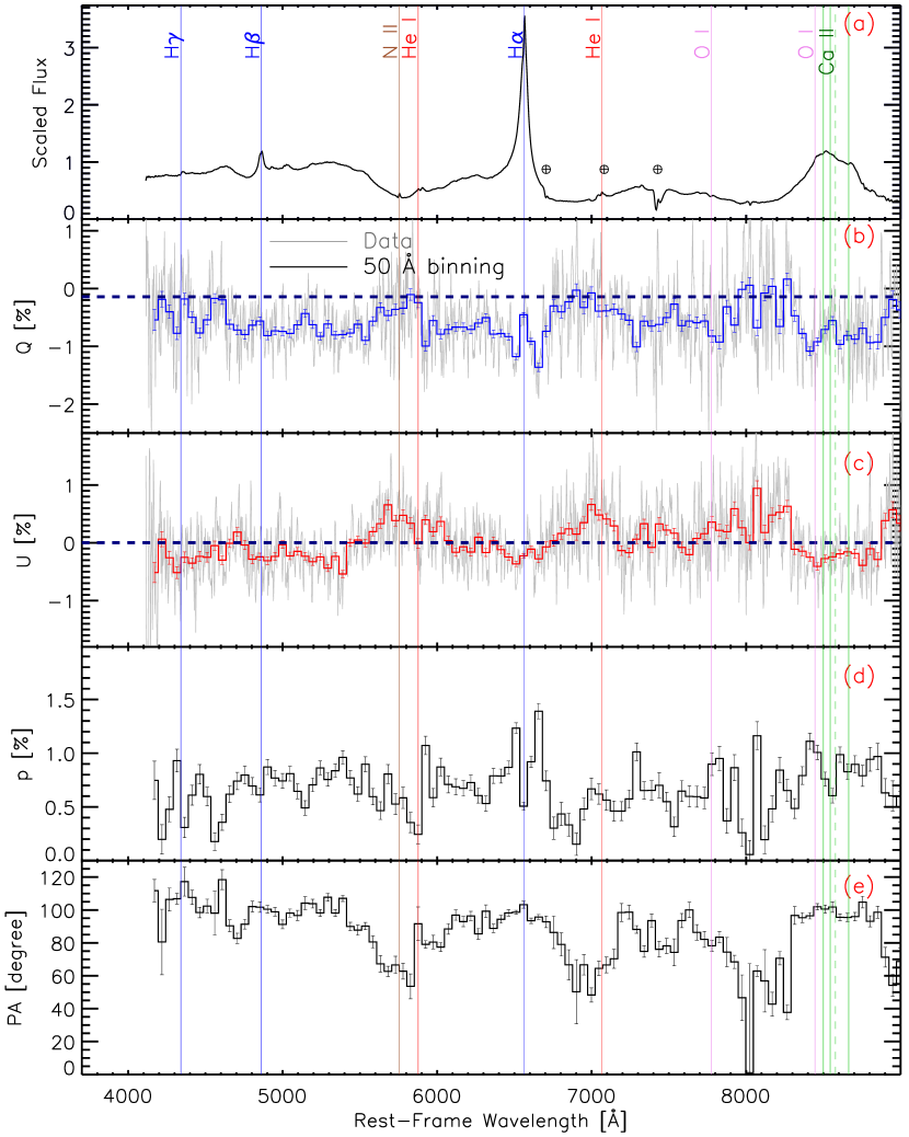
Figure 9: Spectropolarimetry of SN 2018evt on day 172 (epoch 1). The five panels (from top to bottom) give (a) the scaled flux spectrum; (b,c) the normalised Stokes parameters $Q$ and $U$, respectively; (d) the polarization spectrum ($p$); and (e) the polarization position angle PA. Line identifications are provided in the top panel. The data have been rebinned to 50 Å for clarity.

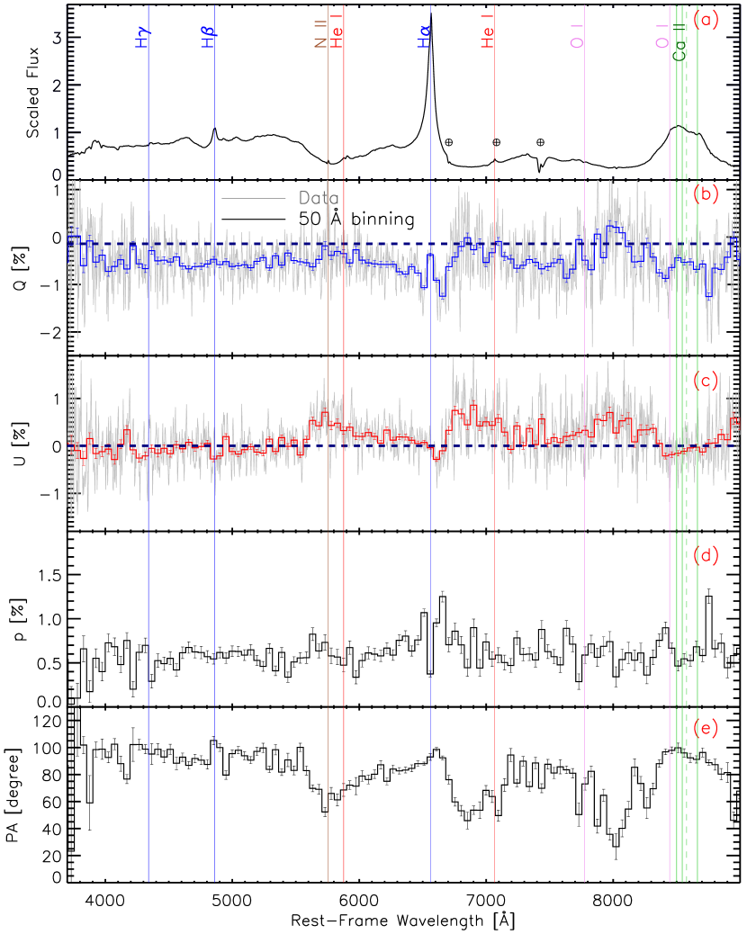
Figure 10: Same as Fig. 9, but for spectropolarimetry of SN 2018evt on day 195 (epoch 2).

The Stokes $Q$ and $U$ values measured by the imaging polarimetry after correcting for the ISP are listed in Table 4. Spectropolarimetry of SN 2018evt obtained at days 172, 195, 198, and 219, together with the associated flux spectra in the rest frame, is visualised in Figures 9 to 12, respectively. Additionally, we compare the $p$ and $PA$ at different epochs in Figure 13, where the amount of polarized flux ($p\times I$) is also presented.

Table 4: VLT/FORS2 imaging polarimetry of SN 2018evt.

UT of Obs.	Phase	Band	$Q_{0}$	$U_{0}$	$Q$	$U$	$p$	PA
	(day)		(%)	(%)	(%)	(%)	(%)	(∘)
2019-01-09 08:26:34	140.4	$b_{\rm HIGH}$	-1.43$\pm$0.09	-0.38$\pm$0.09	-1.29$\pm$0.09	-0.38$\pm$0.09	1.34$\pm$0.12	98.3$\pm$2.5
2019-01-10 08:38:52	141.4	$v_{\rm HIGH}$	-1.49$\pm$0.09	0.02$\pm$0.09	-1.35$\pm$0.09	0.02$\pm$0.09	1.35$\pm$0.12	89.6$\pm$2.5

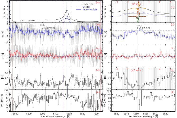
Figure 11: Spectropolarimetry of SN 2018evt obtained on day 198 (epoch 3) and at higher spectral resolution presented similarly as in Fig. 9. The vertical blue line marks H$\alpha$ at zero velocity. The right column portrays the H$\alpha$ emission core between the two vertical purple-dotted lines in the left panel. Vertical grey lines indicate velocities relative to H$\alpha$ in the rest frame in steps of 100 km s^-1. As shown in the fourth panels (d), the polarization reached local maxima at $\sim-2000$ km s^-1 and $\sim 3200$ km s^-1, where flux contributions from the intermediate component are negligible as can be deduced from the profile decompositions in the top panels.

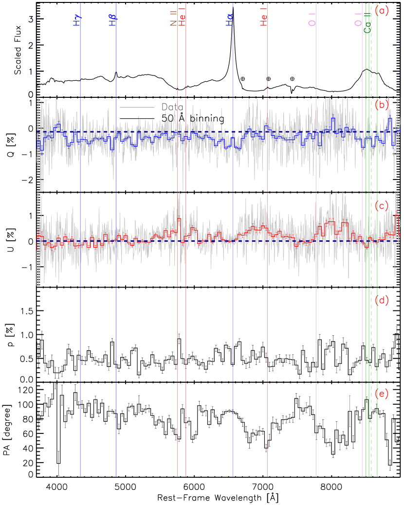
Figure 12: Same as Fig. 9, but for spectropolarimetry of SN 2018evt on day 219 (epoch 4).

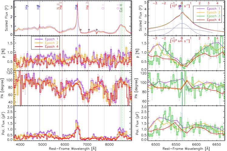
Figure 13: Comparision of the spectropolarimetry of SN 2018evt at different epochs. The left panel shows the observations on epochs 1, 2, and 4 at days 172 (purple), 195 (orange), and 219 (red) in the rest frame, respectively. The four rows present (from top to bottom) the scaled flux spectrum ($I$) with major lines from several species labeled at zero velocity, the degree of polarization ($p$), the polarization position angle (PA), and the polarized flux (the scaled product of $p$ and $I$), respectively. The $p$ and PA data in the left panel have been binned to 50 Å for clarity. The right panel portrays the polarization profile of the H$\alpha$ core on epoch 3 / day 198 (green) with a 3 Å bin size while 15 Å binning was used for the lower-resolution data on epochs 1, 2, and 4. Vertical grey lines indicate velocities in steps of 1000 km s^-1 relative to H$\alpha$.

5.2 The $Q-U$ Plane and Dominant Axes

Similarly to the difference between polar and rectangular coordinates, we present the observations in the $Q-U$ Plane, which is a mathematically convenient alternative to the degree of polarization and polarization position angle. The $Q-U$ plane defined by the Stokes parameters offers an intuitive visualisation of the polarization of the continuum as well as the spectral features (Wang et al., 2001). Each point represents the $Q$ and $U$ values measured in the chosen wavelength bin. Distances to the origin give the degree of polarization, i.e., $p=\sqrt{Q^{2}+U^{2}}$. The azimuth of each data point is directly related to PA$=(1/2)\,{\rm arctan}\,(U/Q)$. Depending on the departure from spherical and axial symmetries, spectral features representing particular chemical distributions may form specific patterns on the $Q-U$ plane.

If the data points (roughly) form a straight line, the PA is about the same at all wavelengths covered, indicating a common symmetry axis in the plane of the sky. Such a straight line on the $Q-U$ plane is known as the dominant axis (Wang et al., 2003; Maund et al., 2010). Any deviation from the dominant axis would be caused by (combinations of) regions of different composition, opacity, or velocity not (fully) sharing the symmetry axis. The dominant axis can be described as

$$U=\alpha+\beta Q.$$ (2)

In general, the SN spectral features arise from a variety of depths in the moving atmosphere and by a variety of processes. The polarization is, therefore, often decomposed into the dominant component $P_{d}$ and the orthogonal one, $P_{o}$, in the perpendicular direction. More details regarding this procedure are described by Wang et al. (2003) and Stevance et al. (2017).

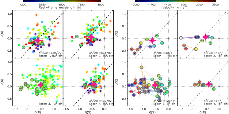
Figure 14: Left: Stokes parameters of SN 2018evt displayed on the $Q-U$ plane. The data have been rebinned to 10 Å for epoch 3 and to 50 Å for the other epochs. In each panel, the wavelength of each bin can be read from the colour bar at the top. The black lines trace the dominant axis computed from the data between 4200 Å and 8800 Å. The solid pink four-point stars identify the continuum polarization deduced over the wavelength range of 4300–6250 Å. The continuum polarization at epoch 3 has been assumed to be the same as at epoch 2 because the observations do not fully cover the continuum reference wavelength region. The larger open grey circles mark the H$\alpha$ region over the velocity range from $-3000$ to $+3500$ km s^-1. Right: same as the left panel but on the H$\alpha$ profile from $-3000$ to $+3500$ km s^-1 with smaller spectral binning as labelled. For the left and the right panels, all data points are coloured according to their wavelength and velocities (respectively), as encoded in the horizontal colour bars.

The left panel of Figure 14 shows the ISP-corrected Stokes parameters on the $Q-U$ plane for all four epochs of our VLT observations. The dominant axis of the SN 2018evt ejecta was determined by performing an inverse-error-weighted linear least-squares fitting of the data. The black long-dashed lines present the dominant polarization axes determined over the wavelength range from 4200 Å to 8800 Å for epochs 1, 2, and 4. Their common slope, $\beta={\rm tan}^{-1}(\theta_{d})$, indicates that the direction on the sky of the symmetry axis tends to be constant from days 173 to 219 ($\theta_{d}\approx 50^{\circ}$; see Table 5). However, although a dominant axis seems to be present at all epochs, we suggest that the large $\chi^{2}$ values per degree of freedom (DoF) as labeled in the lower-right corner of each subpanel imply that the geometry of the ejecta-CSM interaction cannot be well described by a single axial symmetry. Substantial departures on the $Q-U$ plane from a dominant axis can be recognised especially toward shorter wavelengths. This behaviour on the $Q-U$ plane from days 173 to 219 indicates that SN 2018evt belongs to the spectropolarimetic type D1 (Wang & Wheeler, 2008), in which a dominant axis is present with significant scatter of the data points.

The polarization can therefore be decomposed into two components, parallel ($P_{\rm d}$) and orthogonal ($P_{\rm o}$) to the dominant axis. The orthogonal component carries information about departures from the axial symmetry defined by the parallel component. This procedure is equivalent to determining the first two principal components of the polarization (see, for example, Wang et al., 2003; Maund et al., 2010; Stevance et al., 2017). The projected $P_{\rm d}$ and $P_{\rm o}$ at different epochs are shown in Figure 15. Over the three epochs with polarization measurements, the dominant component decreased across the H$\alpha$ wings, the H$\beta$ region and the Ca ii NIR triplet profile. The overall declining $P_{\rm d}$ indicates an increasingly spherically symmetric geometry of the ejecta as more circumstellar H recombines.

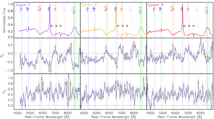
Figure 15: The normalised flux spectra together with the principle-components analysis of the SN 2018evt spectropolarimetry at days 172 (left), 195 (middle), and 219 (right). The top row gives the flux spectra normalised to the maximum value within the observed range. The middle and the bottom rows illustrate the polarization spectra projected onto the dominant axis ($P_{d}$) and the orthogonal axis ($P_{o}$), respectively. The vertical solid lines identify selected spectral features at zero rest-frame velocity. The $\earth$ symbols mark the major telluric features.

5.3 Intrinsic Continuum Polarization

On 2019-01-10 (day $\sim 141$) we detected a linear polarization of $\sim 1.4$% in the $B$ and $V$ bands. This is at a higher level than in the only other SN 1997cy-like event (SN 2002ic) having polarimetry (Wang et al., 2004), which exhibited a $\sim 0.8$% continuum polarization and a $\sim 0.8$% polarization difference between H$\alpha$ and its ambient spectral region. Continuum polarization results from Thomson scattering of free electrons, which is independent of wavelength. After subtracting the ISP as determined in Section 5.1, we arbitrarily selected the wavelength range of 4300–6250 Å, which appears to have no strongly polarized lines, to characterise the continuum polarization. The continuum polarization ($p^{\rm Cont}$) of SN 2018evt at epochs 1, 2, and 4 and the associated position angle (PA^Cont) were derived from the mean of 50 Å binned Stokes spectra weighted by the inverse-squared 1$\sigma$ uncertainties. This error was estimated by adding the uncertainties in the weighted mean (the standard deviation calculated from the same 50 Å binned spectra over the same continuum wavelength range) and the uncertainties in the ISP, in quadrature. Bias correction to the nonnegative $p^{\rm Cont}$ was carried out using Equation 1. Continuum polarizations at the three epochs are listed in Table 5.

We also binned the spectropolarimetry at days 172, 195, and 219 over the b_HIGH and v_HIGH filter passbands that have been used with the imaging polarimetry at days 140/141. This process determines the equivalent imaging polarimetry data points in the b_high and v_high bandpasses. In this way, we formed the polarimetric dataset with the largest possible time baseline. The broad-band polarization was calculated through the integration over wavelength of the filter-transmission-weighted polarized flux. We only consider the uncertainty from the ISP estimation since the spectropolarimetric observations were carried out at very high SNR. The results are given in Table 5. We also present the time evolution of the broad-band polarization and the continuum polarization in Figure 16. The b_HIGH and v_HIGH polarizations have decreased substantially in the time interval days 140/141 to 172 during which the break in the pseudobolometric light curve occurred (see Sec. 3.2). As shown in the bottom panel of Figure 16, we see no strong evidence of time evolution in the polarization position angle, indicating a consistent geometry of the continuum-emitting zone.

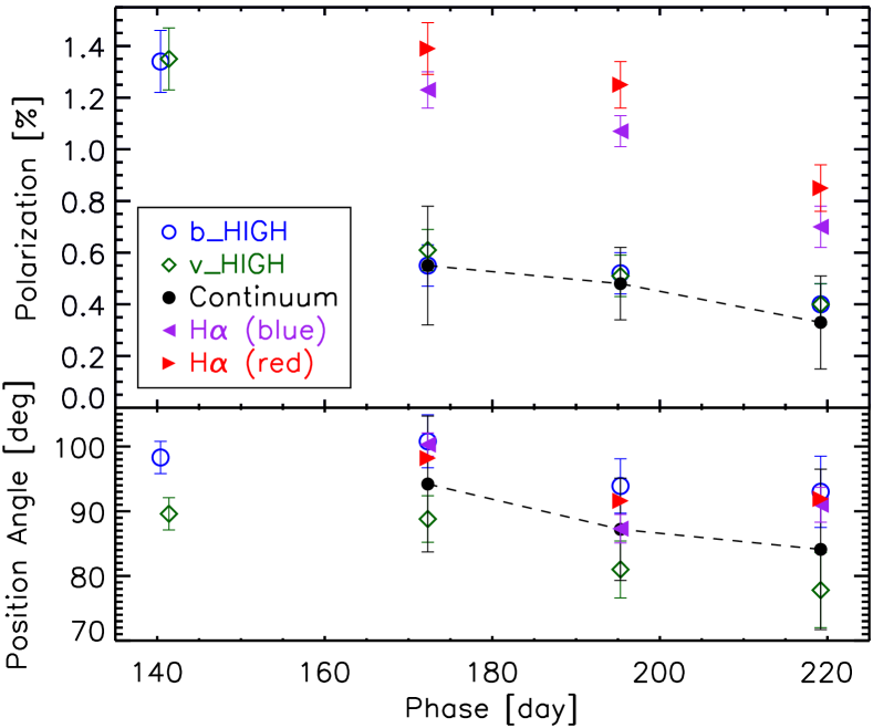
Figure 16: Upper panel: Time evolution of the intrinsic broad-band polarization of SN 2018evt. The presented values include the polarization determined across the VLT b_HIGH and v_HIGH filters, an arbitrarily defined continuum region (4300–6250 Å), as well as the blue and the red wings of the H$\alpha$ emission. Lower panel: The associated temporal evolution of the polarization position angle.

5.4 Intrinsic Polarization of the H$\alpha$ Emission Line

SN 2018evt offers only the second opportunity to date to study the geometry of the H-rich matter of SN 1997cy-like events by spectropolarimetry. Compared to the first case, SN 2002ic (Wang et al., 2004), high-SNR data with a much higher spectral resolution are available for it (Fig. 11). This dataset reveals more details of the prominent H$\alpha$ emission and further enables a more careful interpretation of the nature of the H-rich CSM component.

In addition, one can see that the polarization signal rises more rapidly from the central narrow emission core toward shorter than to longer wavelengths. Such a behaviour is more clearly visible in the right panel of Figure 11, which depicts the wavelength range of 6510–6640 Å and presents the data with a bin size of 3 Å. In the upper panels of Figure 11, we also show the broad and intermediate H$\alpha$ flux components. Furthermore, the narrow absorption and emission components are overplotted in the top-right panel of Figure 11. The maximum polarization level within the narrow absorption component amounts to $\sim 0.6$% in the blue wing of the absorption minimum at around $-$100 to $-$200 km s^-1. This can be understood as the blocking of unpolarized forward-scattered photons from the photosphere along the line of sight. Absorbing material blocks the unpolarized flux, which leads to an increased fraction of the scattering-polarized flux from the asymmetric limb (McCall, 1984).

On day 198, the most prominent H$\alpha$ features in the polarization spectra are significantly polarized line wings and an essentially depolarized core. The latter spans a narrow wavelength range as can be seen in Figures 11 and 13. The widths of the broad and intermediate components are FWHM${}_{\rm broad}^{\rm H\alpha}=7198\pm 34$ km s^-1 and FWHM${}_{\rm int}^{\rm H\alpha}=2291\pm 33$ km s^-1, respectively. Outside the essentially depolarized intermediate component, the peak polarizations were attained as $p_{\rm blue}^{\rm H\alpha}=1.53\pm 0.20$% at $\sim-2000$ km s^-1 ($\sim 2.1\sigma_{\rm broad}^{\rm H\alpha}$) and $p_{\rm blue}^{\rm H\alpha}=1.99\pm 0.34$% at $\sim 3200$ km s^-1 ($\sim 3.3\sigma_{\rm broad}^{\rm H\alpha}$) in the blue and the red wings, respectively. Similar structures can be identified in all other VLT observations (see right panels of Fig. 13). These peak polarization levels in H$\alpha$ are significantly higher than the continuum polarization, i.e., $p^{\rm Cont}=0.48\pm 0.14$%, as estimated in Section 5.3. The corresponding values are also listed in Table 5.

In Figure 16 we also compare the polarization position angle measured in the blue and the red wings of the H$\alpha$ profile. The adopted position angle was that exhibited by the local maximally polarised emission after 50 Å binning. We see neither significant time evolution of the $PA$ nor strong deviation of the $PA$ in the H$\alpha$ wings from the continuum. Therefore, we infer that the ejecta of SN 2018evt and its ambient CSM exhibit similar axial symmetry. Unlike the case of the Type IIn SNe 1997eg (Hoffman et al., 2008) and 2010jl (Patat et al., 2011), the symmetry axes of the SN ejecta and the CSM in SN 2018evt may not be substantially misaligned.

Table 5: Polarization properties of SN 2018evt^(a).

Epoch	Phase	$p^{\rm Cont}$	PACont	$p^{\rm b\_HIGH}$	PACont	$p^{\rm v\_HIGH}$	PAv_HIGH	$p^{\rm H\alpha}_{\rm blue}$	$p^{\rm H\alpha}_{\rm red}$	$\theta^{\rm H\alpha}_{d}$
	(days)	(%)	(degree)	(%)	(degree)	(%)	(degree)	(%)	(%)	(degree)
1(a)	172.3	0.55$\pm$0.23	94.2$\pm$10.5	0.55$\pm$0.08	100.8$\pm$4.1	0.61$\pm$0.08	88.8$\pm$3.6	1.23$\pm$0.07	1.39$\pm$0.10	48.6$\pm$2.0
2(a)	195.3	0.48$\pm$0.14	87.2$\pm$7.9	0.52$\pm$0.08	93.9$\pm$4.2	0.51$\pm$0.08	81.0$\pm$4.4	1.07$\pm$0.06	1.25$\pm$0.09	50.5$\pm$2.3
3(b)	198.2	–	–	–	–	–	–	1.53$\pm$0.20	1.99$\pm$0.34	–
4(a)	219.2	0.33$\pm$0.18	84.1$\pm$12.4	0.40$\pm$0.08	93.0$\pm$5.5	0.40$\pm$0.08	77.8$\pm$5.8	0.70$\pm$0.08	0.85$\pm$0.09	49.1$\pm$3.1

^(a)Measurements of epochs 1, 2, and 4 are based on spectra binned to 50 Å except column $\theta^{\rm H\alpha}_{d}$.
^(b)Measurements of epoch 3 are based on spectra binned to 3 Å.

6 Overview of the Main Observational Properties

The observing campaign on SN 2018evt started at around 110 days past the estimated peak luminosity. At these late times, the SN showed similar multiband absolute magnitudes, decline rates, and spectral evolution as other SN 1997cy-like events (Figs. 2 and 4). In the following, we give a concise overview of the main observational signatures of SN 2018evt. Some of them may not have been identified in earlier SN 1997cy-like events, most prominently the early break in the bolometric light curve, the evolution of the H$\alpha$ and H$\beta$ profiles after day $\sim 100$, the variability of the polarization, and details of the polarization profile of H$\alpha$.

(1) The decline rate of the optical-NIR pseudobolometric luminosity of SN 2018evt increased after day $\sim 170$, which can be seen as a break in Figure 3. To our knowledge, such an early break has not yet been identified in other SN 1997cy-like events, which are only known to exhibit a rapid drop between days $\sim 300$ and 400. Their light curves can be fitted with the equations formulated by Nicholl et al. (2014), which are based on a semianalytic model for the case of ejecta colliding with optically thick CSM (Chatzopoulos et al., 2012). A change in the late-time bolometric luminosity decline rate can be expected if there is a transition of the CSM radial profile from a denser inner region to an outer region with a steep drop in its density. Alternatively, such changes may also be caused by the reverse shock becoming ineffective, so that the forward shock is significantly decelerated. This can happen when the mass of the shocked CSM is comparable to that of the ejecta and the reverse shock is no longer propagating through the ejecta (Svirski et al., 2012).

We point out that the spectropolarimetric observations were only conducted after the first break of the bolometric luminosity; hence, they may not provide insights into the nature of this change. However, the synthesised broad-band polarization at these late epochs is significantly lower than the broad-band polarization measured on day $\sim 140$, obtained $\sim$30 days before the break. Therefore, we do not rule out that the initial luminosity break at day $\sim 170$ could be associated with a significant change of the geometry of the interaction zone between the ejecta and the CSM. Such a break can be caused by the uneven diminishing of the reverse shock if the shocked shell reaches the boundary of the dense part of the CSM (Moriya, 2014). For instance, this can be expected when the shock front has crossed the volume defined by the semiminor axis of a hypothetical dense ellipsoid but has not yet fully traversed the range spanned by the semimajor axis. Follow-up photometry has shown a secondary break in the multiband light curves of SN 2018evt at day $\sim$480 (see Sec. 7.3 and Wang, Lingzhi et al., in prep.). The time and amplitude of bolometric decline-rate variations are essential for modeling the mass and spatial extent of the CSM.

(2) The late-time H$\alpha$ emission can be satisfactorily described by the superposition of a pseudocontinuum and a broad and an intermediate Gaussian component, with widths at day 198 of FWHM${}_{\rm broad}^{\rm H\alpha}=7198\pm 34$ km s^-1 and FWHM${}_{\rm int}^{\rm H\alpha}=2291\pm 33$ km s^-1, respectively. The broad component exhibits conspicuous time evolution while the intermediate component is relatively stationary until day 300 (Figs. 5 and 6). After that, the intermediate component shifts toward longer wavelengths.

(3) The VLT spectrum with higher spectral resolution obtained on day 198 reveals the P Cygni nature of the inner H$\alpha$ profile. The core region can be well fitted by two narrow Gaussian functions characterising the absorption (FWHM $=110\pm 16$ km s^-1) and the emission (FWHM $=133\pm 24$ km s^-1) components. The expansion velocity measured in the absorption component amounts to $v_{\rm wind}=63\pm 17$ km s^-1 (see, e.g., Fig. 8).

(4) As the luminosity of SN 2018evt dropped, the strength of the Balmer lines relative to the underlying continuum increased between days $\sim 125$ and 240. The relative contribution by the blue wing to the total H$\alpha$ line emission decreased nonmonotonically through the end of our spectral series at day 365. The relative intensity of the red wing increased between days $\sim 125$ and 240 (see bottom panels of Figs. 5 and 6).

The changes in line structure were accompanied by a shift of the central peak of the broad H$\alpha$ component from $-1200$ km s^-1 to $\sim+100$ km s^-1 between days 125 and 365. This shift can be understood as follows. The broad H$\alpha$ component is produced in a cold dense shell (CDS) within the region between the forward and reverse shocks (see Section 7.2 for more details). As the ejecta expand over time and become progressively optically thin, the occultation of the red-side emission of H$\alpha$ gradually decreases. This results in an increase in the observed red-wing intensity and leads to a redward shift of the peak of the H$\alpha$ profile. Note that such a behaviour is different from the H$\alpha$ evolution at earlier phases reported for other interacting SNe. For instance, during days $\sim 75$–100, SN 1997cy-like events often show a decreased intensity in the red wing and an increased intensity in the blue wing. These signatures identified at relatively early phases were interpreted as a result of the formation of new dust grains in the shocked material (see, e.g., Lucy et al., 1989 for the first documented case of SN 1987A and Smith et al., 2009; Trundle et al., 2009; Fox et al., 2011; Smith et al., 2012, and Silverman et al., 2013a for SN 1997cy-like events, and Zhang et al., 2021 for the Type II SN 2018hfm).

(5) The continuum polarization of SN 2018evt decreased substantially over time. The $B$- and $V$-band polarizations were both $\sim 1.3$% on day 140. The continuum polarization dropped from $\sim 0.6$% to 0.3% between days 172 and 219. The polarization position angle remained constant within the uncertainties. That is, while the nonsphericity of the ejecta-CSM interaction region decreased with the recession of the photosphere into interior zones, the orientation of this asphericity did not change significantly on the plane of the sky (Figs. 9–12, Table 5).

(6) The narrow central peak of the prominent H$\alpha$ emission line is almost completely unpolarized (Figs. 11 and 13). Such a depolarization probably occurred in an H-recombination zone. The residual low line-of-sight polarization level of $\sim 0.14$% (Fig. 20) has been adopted for the ISP correction. At all four epochs, the peak polarization in the wings is a factor of $\sim 2.5$ higher than the continuum polarization. The position angles across the emission profile are different from those measured in the continuum (Table 5).

Since the intrinsic polarization of the H$\alpha$ recombination core is zero, we attributed a line-of-sight polarization level of 0.14$\pm$0.08% to the ISP (see, Section 5.1 and Appendix C). In other words, if a substantial amount of scattering dust is present in the CSM, an apparent line polarization at the H$\alpha$ emission core would be expected, which is incompatible with the observed low line-of-sight polarization level. Therefore, we infer that the number density of dust grains in the volume within the first $\sim 200$ days is probably insignificant. Furthermore, the asymmetry of the emission-line profiles is intrinsic and not only apparent owing to obscuration by dust. CSM with such a low dust content is consistent with the configuration of the circumstellar environment of the Type IIn SNe 1997eg (Hoffman et al., 2008) and 2010jl (Patat et al., 2011).

(7) The polarization across the H$\alpha$ line was found to increase monotonically from the minimum at the emission peak toward both shorter and longer wavelengths. The polarized flux exhibits an enhancement in the blue wing relative to the red wing as shown in the bottom panels of Figure 13. The peaks of the polarization are outside the intermediate emission component of H$\alpha$, suggesting that the polarized flux is contributed by the broad component while the intermediate component is likely to depolarize the emission. Such a structure was first seen in the H$\alpha$ polarization profile of the Type IIn SN 1998S (Leonard et al., 2000). It can be explained by the fractional contribution of the flux from the polarized continuum increasing toward the edges of the depolarizing intermediate component.

An alternative mechanism that explains the broad component of H$\alpha$ is given by the line-emitting clouds and its large number of fragmented cloudlets. According to the Monte-Carlo calculation based on the late-time observation of the Type IIn SN 2008iy, a large number of small, fragmented clouds ($N_{f}\gtrsim 10^{6}$) is required to account for the observed smoothness of the H$\alpha$ profile, compared to the number of the non-fragmented, shocked clouds ($N_{c}\sim 10^{3}$, Chugai, 2009, 2018, 2021). We suggest that such a configuration is also compatible with the decreased polarization toward the emission center of the H$\alpha$ profile since the flux will become progressively dominated by recombination toward the lower velocities, which is intrinsically unpolarized. The reproduction of the line profile through numerical simulations will be essential to probe the detailed line-forming mechanisms.

Although similar polarization profiles have been identified in the Type IIn SNe 1997eg (Hoffman et al., 2008) and 2010jl (Patat et al., 2011), we do not see strong evidence of a significant difference between the polarization angle over the H$\alpha$ profile and the pseudocontinuum as shown by those other events. The polarization position angle across the H$\alpha$ profile also exhibits little wavelength dependence. Therefore, the continuum-emitting region and the H-rich component may share a similar axial symmetry.

7 Discussion

7.1 Comparison Between SNe IIn and SNe Ia-CSM 

In Table 6, we briefly compare the general observational properties of SNe IIn and SNe Ia-CSM. The core difference between the two types of strongly interacting SNe is obviously whether the underlying explosion has a thermonuclear origin or is due to core collapse. The comparison suggests both similarities and discrepancies. For example, SNe IIn exhibit a bimodal distribution of their rise times, and SNe Ia-CSM are on average more luminous. The identification of strong He i $\lambda$5876 and O i $\lambda$7774 in the late phases of SNe IIn also differentiates the two classes. Moreover, it seems that the wind velocities inferred from the blueshift of narrow P Cygni absorption features in SNe Ia-CSM fall into a narrow and low range ($\sim 50$–100 km s^-1), while SNe IIn exhibit a wider range of wind velocity ($\sim 20$–800 km s^-1). However, the small sample size of long-term polarimetric temporal series of both SNe IIn and SNe Ia-CSM is not (yet) sufficient to deduce any time patterns.

Table 6: Comparison of the general observational properties of SNe IIn and SNe Ia-CSM.

		SNe IIn	SNe Ia-CSM
Light Curve	Rise Time	Fast, 20$\pm$6 d; slow 50$\pm$11 d[a]	20$\lesssim t_{\rm rise}\lesssim 40$ d[b]
		$20\lesssim t_{\rm rise}\lesssim 50$ d[c]
	Peak Mag	$-20\lesssim M_{r}\lesssim-17.8$ mag[a],	$-21.3\lesssim M_{R}\lesssim-19$ mag[b]
		$-19\lesssim M_{R}\lesssim-16$ mag[c]
Spectra	Early	Balmer lines + blue continuum[d]	Balmer lines + SN 1991T-like spectrum
			strong Fe iii, weak/no Ca ii and Si ii
	Late	He i $\lambda$5876	Weak He features[b]
		Prominent O i $\lambda$7774	No strong evidence of O[b]
	Wind Velocity	$20\lesssim v_{\rm wind}\lesssim 800$ km s-1 [e]	$50\lesssim v_{\rm wind}\lesssim 100$ km s-1 [f]
Polarization	Continuum	Around peak, 1.7%$\lesssim p^{\rm Cont}\lesssim 3.0$%[g]	day 141, $p^{\rm Cont}\approx 1.3$%[∗]; $\gtrsim$ day 200, $\lesssim 0.5\%^{[h,*]}$
		Decrease over time[i]	Decrease over time [j,∗]
	Position Angle	Exhibit little time evolution	Same as SN IIn[∗]
	Balmer Lines	Depolarized at the narrow emission core,	Same as SN IIn[∗]
		increase and exceed $p^{\rm Cont}$ toward outer wings
		Higher polarization peak in the red wing[k]
		Misaligned with the ejecta and He-rich CSM[k]	No misalignment between H-rich CSM and ejecta[∗]
	He i	Misaligned with the H-rich CSM,	No He i emission
		aligned with the ejecta[k]

^[a]Nyholm et al. (2020), ^[b]Silverman et al. (2013a), ^[c]Kiewe et al. (2012), ^[d]Filippenko (1997), ^[e]Salamanca et al. (1998); Fassia et al. (2001); Salamanca et al. (2002); Pastorello et al. (2002); Miller et al. (2010); Fransson et al. (2014); Inserra et al. (2014); Fox et al. (2015); Inserra et al. (2016); Andrews et al. (2017); Chugai (2019); Tartaglia et al. (2020); Taddia et al. (2020), ^[f]Kotak et al. (2004); Aldering et al. (2006); Dilday et al. (2012); Silverman et al. (2013b, a), ^[g]Wang et al. (2004), ^[h]Leonard et al. (2000), ^[i]Hoffman et al. (2008), ^[j]Inserra et al. (2014), ^[k]Hoffman et al. (2008), ^[∗]This work.

7.2 The Structure of the SN-CSM Interaction Region

The high continuum polarization is also indicative of significant asphericity of the SN-CSM interaction region. Because both SN 2002ic (Wang et al., 2004) and SN 2018evt exhibited considerable polarization at late times, major departures from spherical symmetry could be an intrinsic property of the SN 1997cy-like events. Moreover, the late-time spectroscopic and spectropolarimetric properties of SNe Ia-CSM and SNe IIn exhibit considerable similarity, suggesting commonality in the configuration of the SN-CSM interaction region of the two classes.

The polarization angle of a given emission component carries information about its geometric orientation. The dominant polarization axis, which is defined over the entire optical range, remained unchanged with time (see Table 5).

blackOne configuration that can produce a wavelength-independent polarization level and a time-invariant polarization position angle is an aspherical ejecta-CSM interaction zone. As the ejecta expand homologously, their scattering opacity decreases as the column density declines. In SN 2018evt, we observed monotonically decreasing levels of polarization across both the continuum and the broad H$\alpha$ wings, which is contradictory to the optically-thick regime ($\tau\textgreater 1$). This is because if $\tau$ is large, the reduction of multiple scattering will first lead to an increase of the continuum polarization until reaching the highest level when $\tau\approx 1$ before the polarization starts to decrease over time (Höflich, 1991). For SN 2018evt, the fact that the continuum polarization decreases from days 172 to 219 can be understood as the expansion of the SN ejecta leading to a continuous reduction in the scattering optical depth. Additionally, one picture that can qualitatively explain the polarization in the H$\alpha$ wings is the presence of an aspherical H-rich circumstellar envelope. The polarization may arise from electron scattering in the aspherical ejecta-CSM interaction zone. However, electron scattering cannot be the only source that shapes the broad H$\alpha$ component; Dopper broadening must play a significant role (see explanation below). As the CDS expands, the flux of the broad H$\alpha$ wings becomes progressively dominated by Doppler broadening while the contribution from electron scattering decreases, resulting in a decrease of the polarization in the broad H$\alpha$ wings.

In the late phases of SN 2018evt, the expansion speed of the CDS can be inferred from the FWHM of the broad H$\alpha$ component (Dessart et al., 2015; Smith, 2017). The rationale is mainly based on the fact that the CDS has become transparent to the radiation from the inner ejecta. Simulations of the spectral line profiles suggest that, at early times, complete thermalisation is taking place in the CDS. This yields a high optical depth and accounts for the majority of line broadening through noncoherent scattering with thermal electrons (Chugai, 2001; Dessart et al., 2009; Dessart et al., 2015). As the CDS expands, thermalisation becomes incomplete over all depths in the CSM, and the profile of the broad component becomes progressively dominated by the broadening from the large-scale velocity of the CDS (Dessart et al., 2009; Dessart et al., 2015; Taddia et al., 2020). For instance, the electron-scattering optical depth drops below 2/3 after day $\sim$350, implying a weak frequency-redistribution mechanism at such late phases (Dessart et al., 2015).

black Taddia et al. (2020) proposed that the intermediate component of the H$\alpha$ line of the Type IIn SN 2013L arises from the pre-ionised gas. Such a region in the unshocked dense CSM is also expanding at the same wind velocity as the narrow H$\alpha$ component ($\sim 100$ km s^-1). The H$\alpha$ emission was broadened to form the intermediate component with FWHM $\approx 1000$ km s^-1 in this optically thick ($\tau\textgreater 1$) region, while the narrow emission peak originates in the outer, optically thin ($\tau\textless 1$) CSM. However, this picture may not be able to account for the H$\alpha$ profile observed in SN 2018evt. The higher-resolution spectrum of SN 2018evt at day 198 shows that the narrow H$\alpha$ component is clearly separated from the underlying intermediate component (see Figure 8 and the upper-right panel of Figure 13), indicating that the latter cannot be developed through broadening by electron scattering in the unshocked CSM expanding at $\sim 63$ km s^-1.

black An alternative scheme which may account for such a discrete central line profile was proposed by (Chugai, 2021) based on late-time observations of the Type IIn SN 2008iy, which shows a narrow P Cygni profile superimposed on an intermediate (FWHM $\approx 2000$ km s^-1) component at day 702. The intermediate component can be interpreted to arise from a zone that contains shocked and fragmented circumstellar clouds (Chugai & Danziger, 1994). These cloud have already been processed by the forward shock but have not been disturbed by the expanding SN ejecta, which corresponds to the CDS. The H$\alpha$-emitting gas inhabits the velocity spectrum covered by the intermediate component, from the high-velocity range that is similar to the shock speed which accelerates the gas in the CSM, to the low-velocity range that represents the region that has not yet fragmented but accelerated through the development of vortical turbulence in shear flows (the Kelvin-Helmholtz instability). The velocity range thus determines the main profile of the intermediate component. Additionally, the smooth H$\alpha$ profile requires a sufficient fragmentation of the shocked circumstellar clouds.

black The narrow component is formed in the unshocked wind outside the CDS. According to the modeling of SN 2008iy at day 702, the wind speed is higher toward the inner region of the CSM owing to the acceleration by the expanding CDS. The pre-shock CSM around SN 2008iy was accelerated to 145 km s^-1 at the inner layers as indicated by the blueshifted absorption component, compared to the 45 km s^-1 wind speed required at the outermost layers as constrained by the emission component (Chugai, 2021). On the contrary, a constant wind speed cannot achieve a satisfactory fit to the emission component (Chugai, 2021).

black While a plausible modeling of SN 2008iy at day 702 requires minimal contribution of the CDS and electron scattering, we note that our high-resolution spectropolarimetry obtained on day 198 is much earlier. At this relatively early phase, the polarization signatures demonstrate a nonnegligible contribution of electron scattering during our observations of SN 2018evt. Evidence includes the temporal evolution of the continuum and the broad H$\alpha$ wing, the progressive depolarization toward the center of the H$\alpha$ line, and the peak in the polarization spectrum on day 198 around $-100$ to $-200$ km s^-1, which is similar to the velocity of the narrow blueshifted absorption minimum. Therefore, the H$\alpha$ profile is likely to be developed through an interplay between electron scattering and the emitting fragmented circumstellar clouds. The former would produce polarization signals, while the latter would produce strong depolarization over the velocity spectrum covered by the cloud fragments since the emitting flux is from recombination rather than scattering. The latter becomes progressively more dominant over time as the ejecta and the CDS expand, causing a decrease of polarized flux in all spectral regions.

black One concern about such an interplay scenario of SN 2018evt is the small amount of variation of the width of the intermediate component from days 125 to 365 (see Figures 5 and 6). The width of the intermediate component is determined by the shock velocity ($v_{\rm sh}$) and density contrast between the cloud ($\rho_{\rm c}$) and intercloud gas ($\rho_{\rm ic}$): $v_{\rm c}\propto v_{\rm sh}/\sqrt{\rho_{\rm c}/\rho_{\rm ic}}$ (Chugai, 2019). As the CDS expands and the shock decelerates, the characteristic speed of the gas in the shocked clouds would also decrease over time. On the other hand, we found that the central depolarization of the H$\alpha$ component favors an emission source in which recombination becomes progressively dominated toward the line center. The velocity coverage of the intermediate H$\alpha$ is also in good agreement with the range between the two polarization peaks identified across the entire H$\alpha$ profile (from $-2000$ km s^-1 to $+3200$ km s^-1; see Figure 13). We remarked that our Gaussian decomposition and fitting of the H$\alpha$ profile of SN 2018evt only serve as a qualitative description to the observations. The actually profiles originating from different zones may conspicuously differ from a Gaussian function. The detailed profile of each component and whether their temporal evolution can be understood under the framework of the fragmented shocked clouds scheme would require extensive numerical simulations.

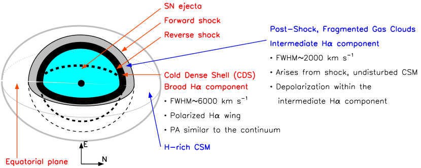
Figure 17: Schematic sketch (not to scale) of the CSM geometry of SN 2018evt viewed from a direction perpendicular to the plane of sky (at a phase of about 1 yr), as explained in Section 7.2. Owing to the lack of evidence to the contrary, the drawing assumes that the SN ejecta and CSM shell are concentric and not tilted with respect to one another.

In Figure 17 we propose a schematic picture of the ejecta-CSM interaction in SN 2018evt. Narrow, intermediate, and broad components of H$\alpha$ were first recognised in the spectrum of SN 1988Z (Filippenko, 1991) and identified by Chugai & Danziger (1994). The basic configuration has been adapted from the sketch of CSM-interacting SNe (for example, Type IIn and Type Ibn) as presented in Figure 1 of Smith (2017).

Figure 17 illustrates the following.
(1) The very inner region consists of the SN ejecta which expand into the CSM.
(2) A forward shock wave was created when the SN exploded and expanded into the ambient CSM. Meanwhile, a reverse shock is propagating into the SN ejecta. blackThe CSM swept up by the forward shock was heated and expanded.
(3) As this reverse shock is propagating inward and heating the inside ejecta, the forward shock moves into the H-rich CSM, creating a photoionised layer. According to the hydrodynamics of shock propagation (Chevalier & Fransson, 1994), the SN ejecta between the forward and the reverse shocks produce a high-density zone and subsequently a low ionisation parameter. Therefore, the gas has a relatively low temperature and was partially ionised. The high-velocity SN ejecta collide with the CSM, resulting in a broad H$\alpha$ emission component (Chugai & Danziger, 1994).
black (4) Gas processed by the forward shock but not yet disturbed was heated and accelerated. A fraction of the gas was fragmented into numerous clumps, developing a broad velocity spectrum of the H$\alpha$ emitting region. Electron scattering would also contribute to the entire H$\alpha$ profile, as indicated by the temporal evolution of the polarization across the continuum and the H$\alpha$ wings, and it becomes progressively less significant as the polarized flux decreased over time.

From error-weighted least-squares fitting of the Stokes $Q-U$ measurements for epochs 1, 2, and 4 (see Fig. 14 and Table. 5), we estimate that $PA^{\rm Cont}\approx 89^{\circ}$. If the continuum polarization arises from an ellipsoidal CSM scattering zone (Höflich, 1991), we conclude that the $PA$ of its semimajor axis is $\sim 179^{\circ}$ on the plane of the sky because it is perpendicular to the $PA^{\rm Cont}$ (see Fig. 17). The continuum-emitting region and the H-rich component have not been distinguished and presented as one axial symmetry in the schematic diagram since no strong evidence of different $PA$ between the pseudocontinuum and across the H$\alpha$ profile has been identified.

In the outer layer of the CSM, the shape of the region will be traced by the direction of the last scattering. In an atmosphere with Thomson scattering by free electrons, the level of polarization measured in SN 2018evt at early times suggests considerable asphericity. For example, with a density distribution following an inverse-square law, $n(r)\propto r^{-2}$, and a close inner boundary of CSM (1% of the radius of the semiminor axis of a hypothetical ellipsoidal CSM configuration), the continuum polarization ($p\approx 1.35$%) at day 141 indicates an axial ratio 0.75 (Höflich, 1991). At days 195 and 219, as the ejecta are moving through the CSM, the polarized flux decreases and the estimated effective axial ratio becomes greater than 0.9. We note that these are only upper limits in the case when the SN is seen from the equator (perpendicular to the axis of symmetry). The true axis ratio could be smaller, which would yield a larger asphericity.

A few weeks after the onset of the interaction between the SN ejecta and CSM, a $\sim 1$–2% continuum polarization developed in the Type IIn SN 201jl. At the same time, the wings became increasingly depolarized from the H$\alpha$ wings toward the rest wavelength of the line centre (Patat et al., 2011).

In SN 2018evt, an almost complete depolarization is also seen at the line centre of the H$\alpha$ profile, since the narrow H$\alpha$ core is formed by photons emitted by the outermost H-rich CSM that experiences no scattering by free electrons (see, e.g., Fig. 18 of Dessart et al., 2015). Such polarization signatures show a remarkable resemblance to SN 2018evt at much later phases. A two-dimensional polarized radiative-transfer model for overluminous interacting SNe adopting a prolate CSM with a certain pole-to-equator density ratio can reproduce the observed polarization properties of SN 2010jl (Dessart et al., 2015). Dragulin & Hoeflich (2016) have developed a semianalytic model for the interaction of spherically symmetric stellar winds with the pre-existing CSM. The exact geometry, density profile, and optical depth of the CSM require detailed modeling that is beyond the scope of this paper. Multidimensional radiation hydrodynamics simulations at different phases are essential to model the time-evolving polarization profile of SN 2018evt and further reveal the detailed structures of interacting SNe.

The above schematic as illustrated in Figure 17 explains the presence of both a broad, polarized H$\alpha$ wing and an intermediate-width, depolarized H$\alpha$ component. blackThe overall configuration of the ejecta-CSM interaction is also consistent with the picture of cloud fragmentation proposed by Chugai et al. (2004), Chugai (2019), and Chugai (2021). The formation of the entire H$\alpha$ profile may be due to the combination of the emission from the CDS, the shocked and fragmented clouds, and electron scattering. Detailed modelling is required to produce a more precise picture of the SN ejecta expanding into the CSM.

The polarization spectrum of the H$\alpha$ emission exhibits an asymmetric profile, and the polarization peak in the red wing is slightly higher than that in the blue wing at all four epochs (Table 5). The reason is that the H$\alpha$ line emission is higher in the blue than in the red wing, owing to the underlying pseudocontinuum ($p$ has already been intensity-normalised). A more meaningful representation is provided by the polarized flux ($p\times I$) shown in the bottom panels of Figure 13. At all four epochs, the polarized flux exhibits an enhancement in the blue wing relative to the red wing. Such a behaviour was also reported for the H$\alpha$ profile of the Type IIn SNe 1997eg (Hoffman et al., 2008) and 2010jl (Patat et al., 2011). The red-wing deficit in the polarized flux may be the result of the flux from the receding half of the scattering region being partially blocked by the approaching side, which can be explained by an ellipsoidal or disk-like CSM configuration that is not face-on to our line of sight.

7.3 CSM Mass Estimate

In this section, we conduct a rough order-of-magnitude estimation of the mass of the CSM around SN 2018evt. We especially focus on the late-time bolometric luminosity, for which we consider the kinetic energy of the SN ejecta as the source of the radiation energy. Therefore, the mass estimated below accounts for the CSM swept up by the expanding explosion shock wave. As discussed in Section 7.2, because the effective axial ratio of the ellipsoidal CSM is $\sim 0.9$ around day 200, a steady, spherically-symmetric mass loss is adopted for simplicity.

The observed late-time luminosity is dominated by the kinetic energy of the SN explosion interacting with the CSM which can be written as $dE_{\rm k}=q_{r}\times 4\pi r_{\rm sh}^{2}dr_{\rm sh}$. Here $r_{\rm sh}$ denotes the radius of a shell of CSM reached by the forward shock with negligible width $dr_{\rm sh}\ll r_{\rm sh}$. The term $q_{r}$ gives the dynamic pressure, or the kinetic energy per unit volume, and can be expressed in terms of the fluid density of the CSM ($\rho_{\rm csm}$) and the flow velocity: $q_{\rm r}=(1/2)\rho_{\rm csm}v_{\rm sh}^{2}$. Thus, the bolometric luminosity becomes $L=\epsilon_{k}\frac{dE_{k}}{dt}=2\pi\epsilon_{k}\rho_{\rm csm}r_{\rm sh}^{2}v_{\rm sh}^{3}$. In this expression, $\epsilon_{k}$ is the conversion efficiency from kinetic energy to radiation, and $v_{\rm sh}$ is the flow speed.

Assuming that the radial density structure of the CSM follows a power law as $\rho_{r}=\rho_{0}r_{\rm sh}^{-s}$, the mass-loss rate can be written as $\dot{M}=4\pi r_{\rm sh}^{2}\rho_{\rm csm}v_{\rm wind}$, where $v_{\rm wind}$ is the velocity of the wind from the progenitor. We remark that for the sake of simplicity, our raw approximation is based on the assumption of a steady, spherically symmetric mass-loss profile. Such a configuration is in contradiction to the implied disk-like CSM concentration from polarimetry. Therefore, the estimated mass of the CSM is more likely an upper limit. More careful modeling is required to investigate the effect of the asymmetric CSM on its mass profile.

In the case of steady mass loss ($s=2$), $\dot{M}$ becomes $4\pi\rho_{0}v_{\rm wind}$, and the bolometric luminosity can be written as $L=\frac{\epsilon_{k}}{2}\frac{\dot{M}}{v_{\rm wind}}v_{\rm sh}^{3}$. Therefore, $\dot{M}=\frac{2Lv_{\rm wind}}{\epsilon_{k}v_{\rm sh}^{3}}$, or

$$\dot{M}=\frac{3.17}{\epsilon_{k}}\bigg{(}\frac{L}{10^{42}\,{\rm erg\,s^{-1}}}\bigg{)}\bigg{(}\frac{v_{\rm wind}}{100\,\rm{km\,s^{-1}}}\bigg{)}\bigg{(}\frac{v_{\rm sh}}{1000\,\rm{km\,s^{-1}}}\bigg{)}^{-3}\times 0.1\,{\rm M}_{\odot}\,{\rm yr^{-1}}.$$ (3)

Because of the presence of significant H$\alpha$ emission as early as day $-9$ (Fig. 4), the CSM has a very small inner radius, $R_{\rm in}$. On day $\sim 365$, when the last optical spectrum presented in this paper was obtained, the residuals of the two-Gaussian component fitting (Fig. 19) suggest that the narrow P Cygni H$\alpha$ profile from the CSM still persisted. A rough lower limit on the outer radius $R_{\rm out}$ of the shell can be placed as

$$R_{\rm out}\approx v_{\rm CDS}\times t_{\rm shock}.$$ (4)

Here, $v_{\rm CDS}$ is the velocity of the CDS at the time of the fast expansion of the SN ejecta into the CSM.

$t_{\rm shock}$ denotes the time elapsed since the SN explosion. Since no significant increase of the decline rate was observed in the late-time bolometric luminosity until $\sim 1$ yr after the estimated maximum light ($\sim 385$ days after shock breakout), we infer that the reverse shock is still crossing the ejecta and the forward shock is still effectively interacting with the H-rich CSM at $t_{\rm shock}\approx 385$ days. Adopting $v_{\rm CDS}=(6580\pm 140)$ km s^-1 (see Fig. 6e), we estimate that $R_{\rm out}\gtrsim(2.19\pm 0.05)\times 10^{16}$ cm.

Therefore, the lower limit on the duration of the mass-loss phase of a hypothetical companion becomes $t_{\rm ml}=\frac{R_{\rm out}}{v_{\rm wind}}$, or

$$t_{\rm ml}=31.7\bigg{(}\frac{R_{\rm out}}{10^{16}\,{\rm cm}}\bigg{)}\bigg{(}\frac{v_{\rm wind}}{100\,{\rm km\,s}^{-1}}\bigg{)}^{-1}\,{\rm yr}.$$ (5)

The mass of the CSM can be estimated as $M_{\rm csm}=\dot{M}t_{\rm ml}$, or

$$M_{\rm csm}=\frac{10.0}{\epsilon_{k}}\bigg{(}\frac{L}{10^{42}\,{\rm erg\,s^{-1}}}\bigg{)}\bigg{(}\frac{v_{\rm sh}}{1000\,\rm{km\,s^{-1}}}\bigg{)}^{-3}\bigg{(}\frac{R_{\rm out}}{10^{16}\,{\rm cm}}\bigg{)}\,{\rm M}_{\odot}.$$ (6)

Finally, we attempt a rough estimate of the mass-loss rate and the total mass of the CSM. Based on the observational properties of SN 2018evt at day $\sim 365$ (when the last spectrum was obtained), and assuming that the mass loss matches a steady-state wind law ($\rho_{\rm csm}\propto r^{-2}$), we adopt log $L\approx 42.44\pm 0.02$ erg s^-1 from Table 10, $v_{\rm sh}\approx v_{\rm CDS}\approx 6580\pm 140$ km s^-1 (see, e.g., Fig. 6e), and $v_{\rm wind}=63\pm 17$ km s^-1 as determined from the P Cygni feature. This leads to a mass-loss rate of $\dot{M}\approx(1.9\pm 0.5)\times 10^{-3}\,/\epsilon_{k}\,{\rm M}_{\odot}$ yr^-1 and a total mass of the CSM of $M_{\rm csm}\approx(0.21\pm 0.03)\,/\epsilon_{k}\,{\rm M}_{\odot}$. The efficiency factor is highly uncertain. Simulations by van Marle et al. (2010) suggest an enhanced conversion efficiency with an increasing density of the circumstellar shell. For instance, a 15–30% of maximum efficiency in converting the kinetic energy of the shock to bolometric luminosity can be reached for a circumstellar shell mass of 10 M_⊙. Therefore, we infer that SN 2018evt experienced an order of $\approx 10^{-2}$ M_⊙ yr^-1 mass-loss rate and exhibit at least an order of $\approx$M_⊙ of CSM.

Obviously, the inferred age and mass of the CSM are highly dependent on the size of the dense circumstellar cloud, which is not well constrained by the current observations. However, a lower limit can be derived from the fact that the latest spectrum about 1 yr after the estimated peak luminosity is still dominated by strong Balmer emission lines. The slowly declining pseudobolometric luminosity observed until day 368 (when the last photometric point was obtained; see Sec. 3) also indicates that the intense mass loss building up the CSM started earlier than the SN explosion, namely at least $t_{\rm shock}^{\rm lim}\approx 385$ days before the last spectrum was obtained. Therefore, lower limits on the duration of the mass loss and the mass of the CSM yields $t_{\rm ml}^{\rm lim}\approx(110\pm 30)$ yr.

SN 2018evt emerged from solar conjunction in Dec. 2019. The latest LCO $Bg^{\prime}Vr^{\prime}i^{\prime}$ photometry shows a convincing light-curve break between 2019-12-14 and 2020-02-08. For example, the $g^{\prime}$ and $r^{\prime}$ light-curve decline rates have changed from $(0.588\pm 0.005)\,(100\,{\rm day})^{-1}$ and $(0.558\pm 0.009)\,(100\,{\rm day})^{-1}$ (between days 170 and 370) to $(1.11\pm 0.11)\,(100\,{\rm day})^{-1}$ and $(1.31\pm 0.07)\,(100\,{\rm day})^{-1}$ (between days 480 and 533), respectively. Although the time evolution of the bolometric luminosity is at best poorly documented owing to the lack of NIR photometry, we tentatively estimate that a secondary break of the SN luminosity evolution occurred around $t^{\prime}_{\rm shock}\approx 500$ days after the explosion. Therefore, the outer bound of the dense CSM becomes $R^{\prime}_{\rm out}\approx(2.84\pm 0.06)\times 10^{16}$ cm. The corresponding duration of the mass loss and the amount of the CSM then become $t^{\prime}_{\rm ml}\approx(143\pm 39)$ yr and $M^{\prime}_{\rm csm}\approx(0.27\pm 0.04)/\epsilon_{k}\,{\rm M}_{\odot}$, respectively. Observational properties of SN 2018evt obtained at even later epochs will be presented in a separate paper (Wang, Lingzhi et al., in prep.).

7.4 Implications of Various Pre-explosion Mass-Loss Models

The inferred mass of the CSM around SN 2018evt of several, and possibly even a few tens, solar masses is in extreme contrast to the upper mass limit ($\lesssim 0.03\,{\rm M}_{\odot}$; Lundqvist et al., 2013) in both SD and DD models for normal SNe Ia that do not exhibit Balmer lines. The following examines various mass-loss mechanisms but dismisses most of them.

The mass-loss rates of massive (3–7 M_⊙) AGB stars appears to be similar tothe above estimates for SN 2018evt (typically in the range of $10^{-8}$ to $10^{-5}$ M_⊙ yr^-1, but reaching up to $>10^{-4}$ M_⊙ yr^-1 in the superwind phase; Höfner & Olofsson, 2018). According to simulations of the evolution of solar-metallicity stars, the mass of an AGB star can be as large as $\sim 11$ M_⊙ with an H mass fraction of $\sim 70$% (Siess, 2006). However, the mechanism driving such intense mass loss within a short time window just prior to the terminal explosion of the companion WD as a SN remains unexplained.

Another way of producing much-enhanced mass loss in a binary system is Roche-lobe overflow (RLOF) at low wind velocity ($\sim 50$ km s^-1; Mohamed & Podsiadlowski, 2007). When the companion fills its Roche lobe, the mass-transfer rate is drastically enhanced (by two orders of magnitude) with respect to a wind, leading to intensive mass loss strongly concentrated toward the orbital plane. Mass transfer by Roche-lobe overflow (RLOF) can efficiently strip a star of its H envelope (Smith, 2014). Meng & Podsiadlowski (2017) proposed that a common envelope could be formed during such a RLOF phase. Moreover, the explosion of hybrid CONe WDs with a nondegenerate companion and within such a massive H-rich common envelope may explain most of the observational features as well as the rates of SNe Ia-CSM (Meng & Podsiadlowski, 2018; Soker, 2019).

The wind velocity of SN 2018evt is very similar to that reported for PTF11kx ($65\pm 10$ km s^-1, Dilday et al., 2012) but only $\sim 1/3$ of that determined for the other two well-studied objects showing remarkably similar photometric and spectroscopic evolution, namely SNe 2012ca (Inserra et al., 2014) and 1999E (Rigon et al., 2003), which were suggested to be core-collapse events. The low wind velocity of SN 2018evt together with a substantial amount of mass loss is consistent with the lower velocity bound of a few tens of km s^-1 during outbursts of LBVs. However, the current modeling suggests an order of magnitude lower mass-loss rate, even with a super-Eddington wind that might be driven by SOME dynamical instability during the final accretion phase to the WD (Meng & Podsiadlowski, 2017, 2018). Therefore, we consider the high mass-loss rate estimated for SN 2018evt may not be compatible with this scenario. A symbiotic nova system also requires that the CSM is highly concentrated in the orbital plane to be consistent with the photometric behaviour (Dilday et al., 2012). The high kinetic energy and large amount of CSM as inferred from the broad H$\alpha$ emission and the slowly evolving photometric and spectroscopic features perhaps suggest that the CSM around SN 2018evt may not have originated from multiple eruptions from a recurrent nova.

Chevalier (2012) discussed the possibility that a compact object may spiral into the central core of its companion star through a common-envelope evolution, which may lead to the explosion of a luminous, long-lasting SN IIn with massive CSM. This mechanism accounts for the delay by tens to hundreds of years in the SN explosion after the intense mass loss (a few $10^{-2}$–$10^{-1}$ M_⊙ yr^-1). This picture may also be compatible with a thermonuclear explosion if the compact object is a WD (Livio & Riess, 2003). Furthermore, the enhanced CSM during the common-envelope phase is concentrated toward the orbital plane of the binary (Terman et al., 1995; Taam & Sandquist, 2000), which is in agreement with the similar axial symmetry suggested by SN 2018evt. Detailed modeling of SN 2018evt will be particularly useful to test whether the common-envelope scheme would be able to account for (1) the polarization and its temporal evolution, and (2) massive CSM ($\sim$ M_⊙), as inferred from observations.

The identification of an LBV progenitor of the nearby Type IIn SN 2005gl in pre-explosion HST images provides a strong clue for SN explosions of LBVs, and indicates heavy mass loss and intense interaction between ejecta and CSM (Gal-Yam et al., 2007). The inferred mass loss of SN 2018evt, $\dot{M}\approx(1.9\pm 0.5)\times 10^{-3}\,/\epsilon_{k}\,{\rm M}_{\odot}$ yr^-1 at a speed of $v_{\rm wind}=68\pm 17$ km s^-1 over a period of at least $t_{\rm ml}\gtrsim(110\pm 30)$ yr, or $t^{\prime}_{\rm ml}\approx(143\pm 39)$ yr, may resemble LBV-like eruptions during about a century before explosion. A single LBV eruption may last from years to a few decades. For example, the 1890 eruption of $\eta$ Car has ejected a total mass of 10–20 M_⊙ within $\sim 20$ yr (Smith et al., 2003; Smith & Ferland, 2007; Smith & Frew, 2011). A long duration of the CSM build-up may require a series of eruptions. The mass loss of SN 2018evt may fall into the LBV giant-eruption regime in Figure 3 of Smith (2017), which illustrates the mass-loss rate as a function of wind velocity.

One extreme case of an SN that exploded inside a massive H-rich envelope is given by the Type IIn SN 2006gy (Smith & Townsend, 2007). Recently, Jerkstrand et al. (2020) proposed that emission lines at day $\sim 400$ of this luminous event (i.e., $M_{R}^{\rm Peak}\approx-21.8$ mag; Smith & Townsend, 2007) are from neutral iron. The large mass of ground-state iron ($\gtrsim 0.3$ M_⊙) expanding at 1500 km s^-1 is unlikely to be produced by a core-collapse explosion for which the expected kinetic energy of the ejecta is an order of magnitude higher. Therefore, Jerkstrand et al. (2020) proposed that SN 2006gy can be understood as a typical SN Ia hitting a dense shell of CSM. If the modelled iron mass of SN 2006gy is correct, it would establish a case of an extensive CSM enrichment preceding a common-envelope evolution that leads to a SN Ia explosion. However, compared to other events that have been classified as SNe Ia-CSM, SN 2006gy has an order-of-magnitude brighter peak luminosity, a much broader light curve, and significantly different spectral evolution. Whether the progenitor systems of various types of SNe interacting with a massive CSM are so heterogeneous is still pending observational tests.

8 Summary

We reported the results of our photometric, spectroscopic, and polarimetric follow-up observations of the SN 1997cy-like SN 2018evt from about 100 days to $\sim 1$ yr after the estimated peak luminosity. We identified an early break in the pseudobolometric luminosity around day 170, followed by a major further acceleration of the decline one year after peak luminosity. Based on a steady mass-loss wind profile, we infer that SN 2018evt exploded inside a massive circumstellar cloud with a lower mass limit $M^{\prime}_{\rm csm}\approx(0.21\pm 0.03)\,/\epsilon_{k}\,{\rm M}_{\odot}$, which may result from a mass-loss rate of $\dot{M}\approx(1.9\pm 0.5)\times 10^{-3}\,{\rm M}_{\odot}$ yr^-1 at a speed of $v_{\rm wind}=68\pm 17$ km s^-1 over a period of at least $t_{\rm ml}\gtrsim(110\pm 30)$ yr.

The polarization properties of SN 2018evt also indicate some geometric similarities to SNe IIn. For example, a high level of continuum polarization ($\sim 2$–3%) and a significant depolarization at the central core of the Balmer lines have also been observed in the Type IIn SNe 1997eg (Hoffman et al., 2008), 1998S (Leonard et al., 2000), and 2010jl (Patat et al., 2011). These features suggest that SNe Ia-CSM and SNe IIn alike possess substantial amounts of CSM with major deviations from spherical symmetry. Furthermore, multi-epoch spectropolarimetry shows that the level of the continuum polarization can decrease between about two weeks and 100 days after the explosion (Hoffman et al., 2008). No strong evidence of misalignment between the symmetry axes of the SN ejecta and the CSM has been identified in our observations.

Furthermore, the polarization of the prominent H$\alpha$ profile consists of a polarized broad wing and a depolarized intermediate core. The former comes from the photons emitted by the high-velocity regions in the inner cold dense shell, and the latter arises from shocked, fragmented, emitting gas clouds that have not been disturbed by the SN ejecta. High-resolution spectropolarimetry has been crucial in unveiling these and other properties of SN 2018evt. Not only does polarimetry achieve low-order spatial resolution regardless of angular size at any distance as long as the flux is sufficient but, at high spectral resolution, it can reveal structures in line profiles that, in total-flux spectra of SNe, are completely washed out by the extreme Doppler broadening.

The formation of a very massive CSM structure within just a century before the explosion is the central challenge for any attempt to model SN 2018evt and similar events involving either core-collapse or thermonuclear explosions. LBV eruptions as well as common-envelope evolution seem to be candidate mechanisms, and both may be realised by nature. LBV eruptions can only be connected to core-collapse events, whereas common-envelope phases may precede both thermonuclear and core-collapse explosions albeit with some preference for the former.

The observational properties of SN 2018evt exhibit a strong resemblance to the known SN 1997cy-like events. However, the exact nature of this event may still remain unclear. The high and evolving polarization signal measured from SN 2018evt can safely rule out any homogeneous mass-loss procedure and the presence of massive spherical shells of the CSM. A significant equator-to-polar mass-loss process of the progenitor system or the pre-existence of an aspherical protoplanetary nebula is favored.

High-resolution spectropolarimetry will continue to be an important tool to characterise the configuration of the massive CSM, which accounts for most of the energy output of SN 2018evt-like events. Additionally, spectroscopy at very late phases, when the optical depth of the interaction zone becomes sufficiently low, will identify unique fingerprints of the explosion physics. Observations and modelling of the line species, the ionisation states, and the line profiles should respectively add to the understanding of the explosion core’s composition, physical conditions, and dynamics, thereby further elucidating the nature of these special events.

Data Availability

The reduced data used in this work may be shared upon request to Yi Yang (yiyangtamu@gmail.com).

Affiliations (Continued)

²¹Department of Astronomy, University of Texas, Austin, TX 78712, USA
²²Purple Mountain Observatory, Chinese Academy of Sciences, Nanjing 210008, China
²³The Raymond and Beverly Sackler School of Physics and Astronomy, Tel Aviv University, Tel Aviv 69978, Israel
²⁴Steward Observatory, University of Arizona, 933 North Cherry Avenue, Tucson, AZ 85721-0065, USA
²⁵Gemini Observatory/NSF’s NOIRLab, 670 N. A’ohoku Place, Hilo, Hawai’i, 96720, USA
²⁶Institute of Space Sciences (ICE, CSIC), Campus UAB, Carrer de Can Magrans, s/n, E-08193 Barcelona, Spain
²⁷Institut d’Estudis Espacials de Catalunya (IEEC), E-08034 Barcelona, Spain
²⁸Physics Department and Tsinghua Center for Astrophysics (THCA), Tsinghua University, Beijing, 100084, People’s Republic of China
²⁹Beijing Planetarium, Beijing Academy of Science and Technology, Beijing, 100044, People’s Republic of China

Appendix A Construction of the Pseudobolometric Light Curve

Based on the absence of significant spectral evolution from days 125 to 365, we consider that a single late-time spectrum adequately represents the major spectral features of SN 2018evt during the late phases for which we obtained photometry. The VLT/FORS2 spectrum of SN 2018evt at epoch 4 (day 219) was used to characterise the shape of the spectral energy distribution (SED) in the optical. An NIR spectrum obtained on day 262 by the NASA Infrared Telescope Facility (IRTF; Rayner et al., 2003) served to represent the spectral shape in the NIR. The details of the NIR spectral properties of SN 2018evt at late phases will be discussed in a forthcoming paper (Lingzhi Wang, et al., in prep).

We dereddened the optical and NIR spectra of SN 2018evt adopting $E(B-V)^{\rm MW}_{\rm 18evt}=0.051$ mag and a Galactic $R_{V}=3.1$ extinction law (Cardelli et al., 1989), scaled the NIR spectrum, and tied it to the red end of the optical spectrum to compensate for the different phases of observation. This procedure creates a composite optical-NIR spectral template. We then performed photometry on this template to obtain synthesised magnitudes in the $Bg^{\prime}Vr^{\prime}i^{\prime}JHK$ bands. Thereafter, a warping procedure was applied to the template to match the difference between the synthesised magnitudes and the actual photometry of SN 2018evt in the AB system after correcting for Galactic extinction. Finally, two pseudobolometric luminosity estimates were obtained at each photometric epoch by integrating the warped spectrum over two wavelength ranges, namely 3870–9000 Å for the optical and 3870–23,200 Å for the optical-NIR.

The SED of SN 2018evt is illustrated in Fig. 18. The wavelength-weighted mean flux densities for each bandpass were computed as $\langle F(\lambda)\rangle=\frac{\int\lambda F_{\lambda}T(\lambda)d\lambda}{\int\lambda T(\lambda)d\lambda}$, as in the STMAG system described by Koornneef et al. (1986). The calculated mean flux densities are also shown in Fig. 18. Here $F_{\lambda}$ and $T_{\lambda}$ represent the flux density in units of erg cm^-1 s^-1 Å^-1 and dimensionless bandpass throughput at a given wavelength $\lambda$, respectively. Since the normalisation was applied to each bandpass individually, the absolute scale of the filter throughput will not affect the computed weighted mean flux density. A more detailed description of the steps is given by Yang et al. (2018a) and Appendix C of Yang et al. (2020).

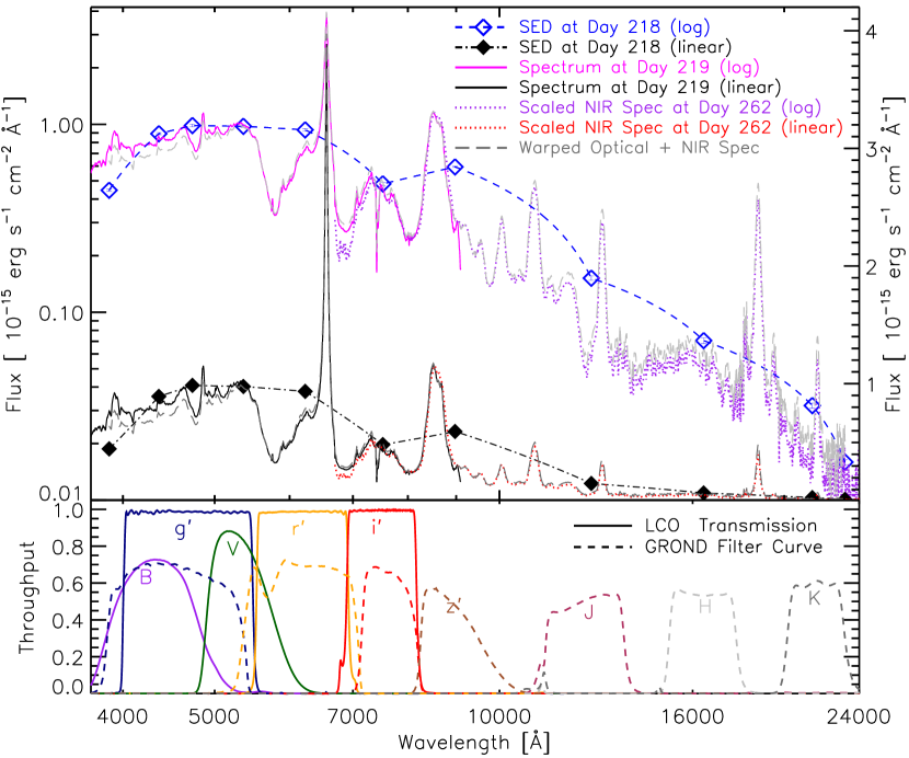
Figure 18: The SED constructed for SN 2018evt. In the upper panel, black diamonds show the flux from the photometry in each bandpass on day 218 at their pivotal wavelengths. The black dot-dashed line outlines the SED obtained by connecting the bandpass monochromatic fluxes. The black solid line and the red-dotted line represent the flux-calibrated VLT spectrum on day 219 and the scaled NIR spectrum on day 262, respectively. The composite optical-NIR spectral template (grey long-dashed line) was warped to match the photometry. The blue, purple, and grey lines and symbols present the same quantities on a logarithmic scale as indicated by the legend. The lower panel depicts the associated bandpass throughput curves. Notice the different shapes between the LCO and the GROND $g^{\prime}$, $r^{\prime}$, and $i^{\prime}$ bandpasses.

Appendix B Fitting the Balmer line profile

To better quantify the H$\alpha$ profile and probe its temporal evolution, we fitted the data as follows. First, we assigned the blue limit ($\lambda_{\rm blue}^{\rm H\alpha}=6330$ Å) and the red limit ($\lambda_{\rm red}^{\rm H\alpha}=6700$ Å) of the region of interest by visually inspecting the data. Second, we determined the pseudocontinuum by fitting a first-order polynomial to the wavelength ranges 6250–6330 Å and 6700–6800 Å. The limits were chosen to avoid any apparent spectral features and telluric absorption. Finally, we subtracted the pseudocontinuum and fitted the spectrum with a multiple Gaussian function, $f_{c}(\lambda)=\sum_{i=1}^{n}A_{i}\ {\rm exp}(-(\lambda_{i}-\lambda_{i}^{\rm rest})^{2}/(2\sigma_{i}^{2}))$. The fitting parameters are the central wavelength in the rest frame ($\lambda_{i}$), the width ($\sigma_{i}$), and the peak height ($A_{i}$) of each component. The results for two Gaussians can be seen in Figure 19.

The VLT flux spectrum at epoch 3 (day 198; also included in Fig. 19) has a higher resolution than the other spectra. It clearly reveals that the narrow H$\alpha$ core exhibits a P Cygni profile, which is unresolved in our other spectra, indicating the existence of a dense and optically thick CSM, into which the SN ejecta are expanding. Because the above two-Gaussian component fitting does not account for the contributions from this P Cygni profile, overt residuals up to $\sim 6$% arose around the line centre. However, the overall residuals across the wings ($\lesssim 2$%) and the RMS value over the entire fitting range ($\lesssim 1.5$%) are both small. Therefore, we suggest that outside the central region dominated by the very narrow P Cygni profile, the late-time H$\alpha$ emission of SN 2018evt is satisfactorily described by a combination of a broad and an intermediate Gaussian component.

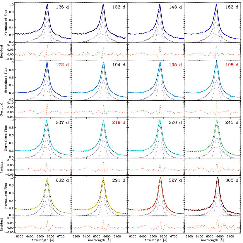
Figure 19: Two-Gaussian component fitting of the late-time H$\alpha$ profile of SN 2018evt. All spectra were resampled to the pixel size of the FLOYDS/LCO spectra, $\sim 1.7$ Å. In each subpanel, grey dotted, purple dot-dashed, and blue dashed lines represent the fits to the pseudocontinuum and to the broad and intermediate Gaussian components, respectively. The black dashed line presents the sum of these three components which tracks the fitted total-flux spectrum as shown by the colour-coded, solid curves. The lower subpanels display the corresponding residuals.

.

Appendix C Estimation of the Interstellar Polarization

Determining the minimal polarization in a spectral line is difficult, especially when noise and limited spectral resolution combine. The measurements will be biased toward higher levels if the line is not spectrally resolved. Our VLT spectropolarimetry at epoch 3 was conducted with a spectral resolution $R\approx 2140$ (3 Å FWHM) at a sampling of 0.73 Å pixel^-1. Such a relatively high spectral resolution enables a more thorough investigation of the ISP than is possible from low-resolution observations (see, e.g., Wang et al., 2004).

In order to quantify the effect of spectral resolution on the measured polarization, we determined the minimum polarization across the H$\alpha$ emission core in the Stokes spectra using various bin sizes. We chose a number of bin sizes $\Delta\lambda>13.3$ Å for the 300V grism configuration ($R\approx 440$) applied at epochs 1, 2, and 4, and $\Delta\lambda>3.0$ Å for the 1200R grism setup used at epoch 3. This operation was performed on the flux spectra obtained at each half-wave retarder-plate angle. The minimum polarization levels across the H$\alpha$ emission core determined with different $\Delta\lambda$ are presented in Figure 20. As shown in the right panel, the minimum polarization levels at epoch 3 tend to be constant for $3\leq\Delta\lambda\leq 10$ Å. A sharp increase from 15 Å and larger implies that the true level of the ISP is represented by the polarization binned to 3 to 10 Å.

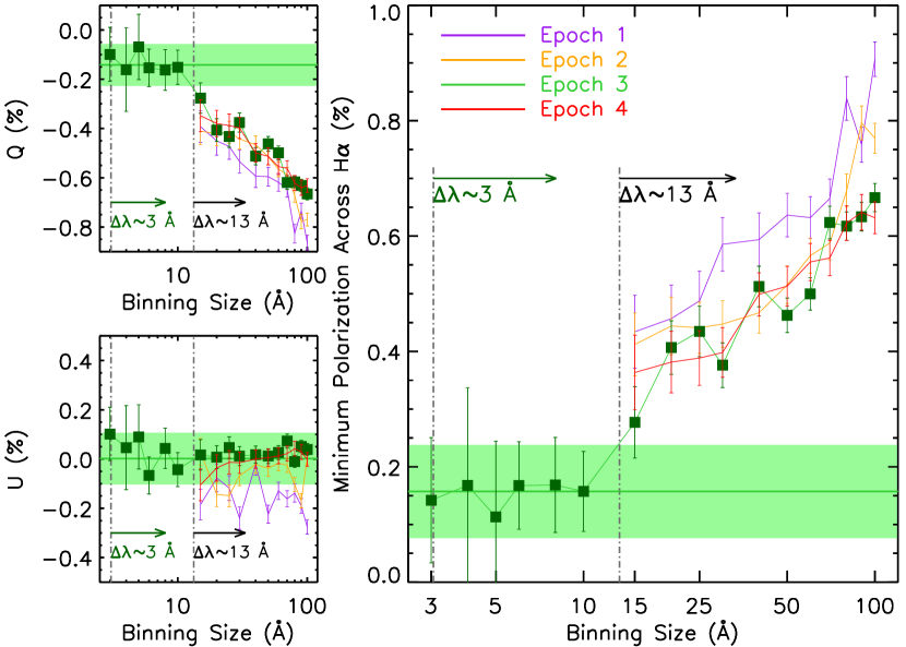
Figure 20: The minimum polarization measured across the H$\alpha$ emission peak as a function of bin size (right panel). In each panel, vertical dot-dashed lines indicate the size of the resolution element in the observations, i.e., $\Delta\lambda\approx 13$ Å for epochs 1, 2, and 4, and $\Delta\lambda\approx 3$ Å for epoch 3. The small scatter exhibited by the dark-green filled squares in all panels suggests that the polarization measured with bin sizes of 3–10 Å corresponds to the actual ISP level if SN 2018evt is intrinsically unpolarized in the narrow H$\alpha$ emission peak. The weighted mean value and the errors estimated in the main text are indicated by the green shaded areas.

We calculated means of the Stokes $Q$ and $U$ parameters over the range of bin sizes that minimise the polarization across the narrow emission peak in H$\alpha$, weighting each spectral element by the inverse square of its 1$\sigma$ error. The arbitrarily chosen bin sizes were 3, 4, 5, 6, 8, and 10 Å. Uncertainties were estimated by adding the associated errors in the error-weighted mean, the error-weighted standard deviation, and the uncertainty in the 10 Å measurement in quadrature. The first two terms can be found as Equations 17 and 18 (respectively) of Yang et al. (2018b). In this way, we derived $q_{\rm ISP}=-0.14\pm 0.08$% and $u_{\rm ISP}=0.00\pm 0.10$%, yielding $p_{\rm ISP}=0.14\pm 0.08$%, and PA${}_{\rm ISP}=89\aas@@fstack{\circ}{6}\pm 15\aas@@fstack{\circ}{4}$. For the estimation of the uncertainties, the covariance matrix of the Stokes parameters has been taken into account following Appendix F of Montier et al. (2015).

Table 7: LCO $Bg^{\prime}Vr^{\prime}i^{\prime}$ photometry of SN 2018evt.

Phasea	MJD	$B$ (mag)	MJD	$V$ (mag)	MJD	$g^{\prime}$ (mag)	MJD	$r^{\prime}$ (mag)	MJD	$i^{\prime}$ (mag)
124.328	58476.328	16.967(013)	58476.332	16.362(011)	58476.336	16.588(008)	58476.344	16.178(009)	58476.348	16.308(013)
124.328	58476.328	16.980(013)	58476.336	16.361(012)	58476.340	16.591(009)	58476.344	16.182(010)	58476.348	16.313(014)
134.688	58486.688	16.976(010)	58486.691	16.377(009)	58485.309	16.599(012)	58485.309	16.131(013)	58485.312	16.241(019)
134.688	58486.688	17.018(011)	58486.691	16.382(008)	58486.691	16.613(006)	58485.312	16.145(014)	58485.316	16.244(021)
139.688	58491.688	17.008(010)	58491.691	16.392(017)	58486.695	16.598(007)	58486.695	16.166(007)	58486.699	16.303(009)
139.688	58491.688	16.989(017)	58491.691	16.376(024)	58491.691	16.634(027)	58486.699	16.166(006)	58486.703	16.314(011)
144.656	58496.656	16.994(022)	58496.660	16.396(013)	58491.695	16.625(013)	58491.695	16.245(031)	58491.699	16.332(018)
144.660	58496.660	17.062(018)	58496.664	16.400(015)	58496.664	16.641(010)	58491.699	16.203(025)	58491.703	16.289(013)
149.254	58501.254	17.057(016)	58501.258	16.399(012)	58496.668	16.617(010)	58496.668	16.120(009)	58496.672	16.339(014)
149.258	58501.258	17.043(018)	58501.262	16.426(011)	58501.262	16.623(009)	58496.672	16.161(008)	58496.672	16.317(014)
154.398	58506.398	17.086(036)	58506.402	16.470(024)	58501.266	16.649(009)	58501.266	16.208(009)	58501.270	16.385(013)
154.402	58506.402	17.148(036)	58506.406	16.388(022)	58506.406	16.601(016)	58501.270	16.204(010)	58501.270	16.395(013)
163.285	58515.285	17.062(009)	58515.289	16.457(011)	58506.410	16.617(016)	58506.410	16.192(016)	58506.414	16.374(025)
163.289	58515.289	17.066(010)	58515.293	16.466(011)	58515.293	16.658(022)	58506.410	16.213(015)	58506.414	16.357(025)
163.301	58515.301	17.102(010)	58515.305	16.468(011)	58515.305	16.702(009)	58515.309	16.239(011)	58515.312	16.419(017)
163.301	58515.301	17.104(011)	58515.305	16.500(008)	58515.309	16.694(008)	58515.312	16.233(011)	58515.316	16.423(015)
177.207	58529.207	17.137(009)	58529.207	16.515(009)	58529.211	16.749(007)	58529.215	16.266(008)	58529.219	16.510(013)
177.207	58529.207	17.106(011)	58529.211	16.509(009)	58529.215	16.765(007)	58529.215	16.276(009)	58529.219	16.518(014)
190.559	58542.559	17.210(016)	58542.562	16.653(009)	58542.566	16.834(006)	58542.570	16.335(007)	58542.570	16.611(021)
190.559	58542.559	17.208(014)	58542.562	16.615(009)	58542.566	16.832(007)	58542.570	16.312(008)	58542.574	16.579(025)
197.281	58549.281	17.312(012)	58549.285	16.643(010)	58549.285	16.877(008)	58549.289	16.372(010)	58549.293	16.605(012)
197.281	58549.281	17.311(012)	58549.285	16.635(009)	58549.289	16.869(008)	58549.293	16.351(010)	58549.293	16.635(013)
204.855	58556.855	17.279(019)	58556.859	16.646(014)	58556.859	16.882(014)
204.855	58556.855	17.309(018)	58556.859	16.659(014)	58556.863	16.894(014)
211.004	58563.004	17.264(027)	58563.008	16.680(021)	58563.008	16.892(019)	58563.012	16.365(020)	58563.016	16.708(027)
211.004	58563.004	17.264(027)	58563.008	16.626(022)	58563.012	16.893(022)	58563.016	16.381(022)	58563.016	16.656(030)
217.863	58569.863	17.362(015)	58569.867	16.718(016)	58569.867	16.975(018)	58569.871	16.435(021)	58569.875	16.724(023)
217.863	58569.863	17.357(014)	58569.867	16.726(018)	58569.871	16.955(016)	58569.875	16.419(016)	58569.875	16.745(020)
225.406	58577.406	17.424(015)
225.410	58577.410	17.438(015)
227.109	58579.109	17.460(016)	58579.109	16.829(011)	58579.113	17.057(009)	58579.117	16.519(011)	58579.121	16.826(015)
227.109	58579.109	17.478(014)	58579.113	16.810(011)	58579.117	17.050(008)	58579.117	16.485(009)	58579.121	16.857(013)
233.484	58585.484	17.498(012)	58585.488	16.864(010)	58585.492	17.091(007)	58585.496	16.562(007)	58585.500	16.911(013)
233.488	58585.488	17.520(011)	58585.492	16.851(009)	58585.496	17.083(006)	58585.496	16.564(008)	58585.500	16.886(013)
242.098	58594.098	17.529(022)	58594.102	16.911(016)	58594.105	17.128(015)	58594.105	16.558(011)	58594.109	16.907(018)
242.098	58594.098	17.577(025)	58594.102	16.873(016)	58594.105	17.131(014)	58594.109	16.561(011)	58594.113	16.940(019)
244.219	58596.219	17.591(013)	58596.223	16.904(009)	58596.227	17.137(008)	58596.230	16.591(008)	58596.234	16.971(012)
244.219	58596.219	17.552(013)	58596.223	16.893(011)	58596.230	17.172(008)	58596.234	16.590(007)	58596.238	16.879(012)
252.832	58604.832	17.548(017)	58604.836	16.877(020)	58604.840	17.166(023)	58604.848	16.593(023)	58604.848	16.937(033)
252.836	58604.836	17.578(018)	58604.840	16.960(026)	58604.844	17.173(021)	58604.848	16.636(027)	58604.852	16.956(029)
260.566	58612.566	17.685(009)	58612.570	17.013(009)	58612.574	17.269(009)	58612.582	16.716(010)	58612.586	17.067(013)
260.570	58612.570	17.696(009)	58612.574	17.013(009)	58612.578	17.253(009)	58612.582	16.719(010)	58612.586	17.083(012)
269.367	58621.367	17.755(032)	58621.371	17.137(071)	58621.379	17.304(031)	58621.379	16.740(016)	58621.383	17.116(025)
269.367	58621.367	17.706(029)					58621.383	16.754(016)	58621.387	17.140(029)
277.508	58629.508	17.784(009)	58629.512	17.092(009)	58629.516	17.346(008)	58629.520	16.800(008)	58629.523	17.172(013)
277.508	58629.508	17.770(010)	58629.512	17.098(009)	58629.520	17.350(008)	58629.523	16.804(009)	58629.527	17.178(013)
285.727	58637.727	17.788(010)	58637.734	17.151(011)	58637.738	17.382(009)	58637.742	16.795(009)	58637.746	17.186(016)
285.730	58637.730	17.786(009)	58637.734	17.149(011)	58637.738	17.384(010)	58637.742	16.801(009)	58637.746	17.207(015)
313.066	58665.066	17.987(011)	58665.070	17.338(011)	58665.074	17.571(009)	58665.082	17.021(011)	58665.086	17.414(015)
313.070	58665.070	17.980(011)	58665.074	17.335(010)	58665.078	17.574(009)	58665.082	17.027(010)	58665.086	17.422(015)
328.719	58680.719	18.035(024)	58680.727	17.409(019)	58680.730	17.619(014)	58680.738	17.083(013)	58680.746	17.488(019)
328.723	58680.723	18.079(025)	58680.730	17.374(017)	58680.734	17.643(014)	58680.742	17.090(013)	58680.750	17.509(021)
346.996	58698.996	18.200(014)	58699.004	17.535(012)	58699.012	17.754(008)	58699.020	17.233(012)	58699.023	17.672(018)
347.000	58699.000	18.218(013)	58699.008	17.535(012)	58699.016	17.733(009)	58699.020	17.230(010)	58699.027	17.597(018)
367.746	58719.746	18.292(016)	58719.754	17.678(017)	58719.762	17.840(010)	58719.770	17.322(010)	58719.773	17.753(018)
367.750	58719.750	18.287(017)	58719.758	17.672(015)	58719.766	17.861(009)	58719.770	17.314(009)	58719.777	17.803(021)

^aDays after $B$-band maximum on MJD 58352.

Table 8: GROND $grizJHK$ photometry of SN 2018evt.

Phasea	MJD	$g$ (mag)	$r$ (mag)	$i$ (mag)	$z$ (mag)	$J$ (mag)	$H$ (mag)	$K$ (mag)
141.324	58493.324	16.522(004)	16.227(002)	16.322(004)	15.822(004)	15.548(029)	15.208(033)	14.986(022)
152.293	58504.293	16.569(019)	16.250(008)	16.359(008)	15.842(009)	15.554(028)	15.353(038)	15.029(032)
161.340	58513.340	16.520(010)	16.203(007)	16.308(008)	15.782(009)	15.549(026)	15.232(020)	15.105(036)
168.305	58520.305	16.621(007)	16.310(005)	16.420(008)	15.882(007)	15.701(021)	15.303(025)	15.268(032)
174.387	58526.387	16.648(009)	16.315(004)	16.462(006)	15.889(005)	15.716(021)	15.411(025)	15.165(040)
182.352	58534.352	16.694(015)	16.350(010)	16.521(013)	15.940(009)	15.787(043)	15.438(049)	15.059(056)
188.207	58540.207	16.737(007)	16.377(004)	16.558(006)	15.966(007)	15.692(037)	15.603(044)	15.333(038)
196.305	58548.305	16.770(007)	16.425(008)	16.583(010)	16.011(007)	15.887(047)	15.463(045)	15.371(036)
211.215	58563.215	16.885(019)	16.495(009)	16.686(010)	16.090(009)	15.947(035)	15.716(040)	15.681(041)
219.227	58571.227	16.910(006)	16.540(005)	16.730(006)	16.135(006)	15.999(029)	15.778(040)	15.629(035)
228.352	58580.352	16.973(004)	16.577(004)	16.796(005)	16.171(004)	16.035(030)	15.817(045)	15.699(034)
234.211	58586.211	17.001(007)	16.622(007)	16.839(006)	16.231(007)	16.018(035)	15.979(067)	15.686(038)
238.230	58590.230	17.019(011)	16.642(010)	16.861(010)	16.249(008)
256.176	58608.176	17.132(004)	16.725(004)	16.971(005)	16.344(005)
272.094	58624.094	17.235(006)	16.820(004)	17.070(004)	16.463(004)	16.274(021)	16.103(023)	15.982(032)
287.125	58639.125	17.344(006)	16.913(008)	17.186(007)	16.568(006)	16.264(050)	16.252(069)	15.986(097)
297.000	58649.000	17.380(011)	16.967(004)	17.235(006)	16.623(005)	16.431(018)	16.277(020)	16.208(045)
303.027	58655.027	17.383(006)	16.976(008)	17.320(009)	16.677(005)	16.354(042)	16.369(056)	16.351(102)
314.027	58666.027	17.503(004)	17.091(001)	17.375(003)	16.752(004)	16.627(025)	16.505(028)	16.286(041)
324.996	58676.996	17.570(010)	17.164(006)	17.449(008)	16.848(008)	16.775(033)	16.481(034)	16.220(063)
354.012	58706.012	17.753(006)	17.360(003)	17.686(005)	17.025(004)	16.839(036)		16.313(046)
369.008	58721.008	17.848(003)	17.464(003)	17.777(004)	17.129(004)	16.970(026)	16.734(030)	16.377(057)

^aDays after $B$-band maximum on MJD 58352.

Table 9: ZTF $g$ and $r$ photometry of SN 2018evt.

Phasea	Filter	MJD	AB Mag	Error
104.563	$r$	58456.563	16.61	0.16
105.550	$r$	58457.550	16.31	0.02
105.555	$r$	58457.555	16.27	0.02
105.561	$r$	58457.561	16.37	0.03
105.566	$r$	58457.566	16.37	0.04
112.555	$r$	58464.555	16.32	0.03
112.560	$r$	58464.560	16.30	0.03
112.565	$r$	58464.565	16.23	0.03
112.570	$r$	58464.570	16.37	0.05
113.558	$r$	58465.558	16.31	0.03
113.563	$r$	58465.563	16.28	0.03
113.568	$r$	58465.568	16.32	0.04
116.540	$r$	58468.540	16.24	0.02
124.541	$r$	58476.541	16.22	0.04
129.544	$r$	58481.544	16.22	0.03
135.498	$g$	58487.498	16.58	0.03
140.499	$r$	58492.499	16.24	0.04
140.534	$g$	58492.534	16.55	0.03
151.502	$r$	58503.502	16.29	0.06
154.507	$g$	58506.507	16.61	0.04
160.522	$r$	58512.522	16.29	0.11
172.436	$g$	58524.436	16.64	0.04
188.336	$r$	58540.336	16.42	0.04
188.440	$g$	58540.440	16.81	0.03
191.481	$g$	58543.481	16.83	0.05
205.360	$r$	58557.360	16.48	0.04
208.397	$r$	58560.397	16.49	0.04
216.335	$r$	58568.335	16.59	0.10
221.403	$r$	58573.403	16.52	0.04
230.272	$r$	58582.272	16.59	0.04
230.353	$g$	58582.353	17.03	0.05
233.273	$g$	58585.273	17.03	0.05
233.314	$r$	58585.314	16.59	0.03
236.314	$g$	58588.314	17.13	0.08
236.361	$r$	58588.361	16.74	0.09
242.252	$g$	58594.252	17.05	0.06
242.335	$r$	58594.335	16.65	0.05
245.293	$g$	58597.293	17.12	0.04
245.376	$r$	58597.376	16.65	0.05
249.232	$g$	58601.232	17.12	0.04
255.247	$r$	58607.247	16.70	0.04
255.295	$g$	58607.295	17.17	0.04
265.196	$g$	58617.196	17.21	0.04
265.272	$r$	58617.272	16.76	0.04
280.286	$r$	58632.286	16.84	0.04
282.233	$g$	58634.233	17.31	0.05
282.234	$g$	58634.234	17.31	0.05
282.273	$r$	58634.273	16.88	0.05
282.286	$r$	58634.286	16.85	0.04
285.189	$r$	58637.189	16.89	0.04
285.231	$g$	58637.231	17.34	0.05
288.190	$g$	58640.190	17.35	0.05
288.210	$r$	58640.210	16.90	0.05
291.191	$g$	58643.191	17.40	0.04
291.232	$r$	58643.232	16.91	0.05
297.233	$r$	58649.233	17.01	0.05
300.190	$g$	58652.190	17.48	0.04
300.274	$r$	58652.274	17.02	0.05
316.172	$r$	58668.172	17.09	0.05
316.190	$g$	58668.190	17.58	0.04
319.206	$r$	58671.206	17.12	0.04
325.170	$g$	58677.170	17.55	0.05
325.190	$r$	58677.190	17.10	0.05
328.192	$g$	58680.192	17.63	0.07
328.235	$r$	58680.235	17.20	0.05

^aDays after $B$-band maximum on MJD 58352.

Table 10: Pseudobolometric luminosities of SN 2018evt.

Phasea	log $L^{b}$ (Opt–NIR)	log $L^{b}$ (Opt)
(Day)	[log (erg s-1)]	[log (erg s-1)]
124.3	42.960(021)	42.791(019)
134.7	42.948(021)	42.783(019)
139.7	42.939(021)	42.777(019)
144.7	42.935(021)	42.776(019)
149.3	42.927(021)	42.769(019)
154.4	42.922(021)	42.762(020)
163.3	42.920(021)	42.757(019)
177.2	42.889(021)	42.732(019)
190.6	42.855(021)	42.700(019)
197.3	42.843(021)	42.686(019)
204.9	42.824(021)	42.672(019)
211.0	42.811(021)	42.664(019)
217.9	42.793(021)	42.648(019)
225.4	42.776(021)	42.628(019)
227.1	42.772(021)	42.623(019)
233.5	42.757(021)	42.605(019)
242.1	42.737(021)	42.584(019)
244.2	42.735(021)	42.583(019)
252.8	42.722(021)	42.572(019)
260.6	42.701(021)	42.550(019)
269.4	42.678(022)	42.526(020)
277.5	42.661(021)	42.509(019)
285.7	42.649(021)	42.498(019)
313.1	42.573(021)	42.434(019)
328.7	42.520(021)	42.378(019)
347.0	42.486(021)	42.350(020)
367.8	42.437(021)	42.303(020)

^aDays after $B$-band maximum on MJD 58352.
^bUncertainty in the distance not included.

Table 11: H$\alpha$ luminosity of SN 2018evt.

Phasea	log $L_{H\alpha}^{b}$
(Day)	[log (erg s-1)]
124.6	41.5331(0192)
132.7	41.4965(0192)
142.6	41.5204(0192)
152.6	41.5194(0194)
172.3	41.5897(0191)
194.4	41.5483(0191)
195.3	41.5345(0191)
207.5	41.5388(0192)
219.2	41.5371(0190)
220.5	41.5171(0190)
244.7	41.4835(0191)
262.4	41.4351(0190)
291.4	41.3919(0191)
327.3	41.3149(0192)
365.4	41.2207(0192)

^aDays after $B$-band maximum on MJD 58352.
^bUncertainty in the distance not included.

References

- Aldering et al. (2006) Aldering G., et al., 2006, ApJ, 650, 510
- Anderson (2018) Anderson J. et al., 2018, EUROPEAN SOUTHERN OBSERVATORY, Doc. No. VLT-MAN-ESO-13100-1543
- Andrews et al. (2017) Andrews J. E., Smith N., McCully C., Fox O. D., Valenti S., Howell D. A., 2017, MNRAS, 471, 4047
- Appenzeller et al. (1998) Appenzeller I., et al., 1998, The Messenger, 94, 1
- Avila et al. (1997) Avila G., Rupprecht G., Beckers J. M., 1997, in Ardeberg A. L., ed., Society of Photo-Optical Instrumentation Engineers (SPIE) Conference Series Vol. 2871, PROCSPIE. pp 1135–1143, doi:10.1117/12.269000
- Bellm et al. (2019) Bellm E. C., et al., 2019, PASP, 131, 018002
- Benetti et al. (2006) Benetti S., Cappellaro E., Turatto M., Taubenberger S., Harutyunyan A., Valenti S., 2006, ApJL, 653, L129
- Blondin & Tonry (2007) Blondin S., Tonry J. L., 2007, ApJ, 666, 1024
- Bochenek et al. (2018) Bochenek C. D., Dwarkadas V. V., Silverman J. M., Fox O. D., Chevalier R. A., Smith N., Filippenko A. V., 2018, MNRAS, 473, 336
- Branch & Wheeler (2017) Branch D., Wheeler J. C., 2017, Supernova Explosions, doi:10.1007/978-3-662-55054-0.
- Brown et al. (2013) Brown T. M., et al., 2013, PASP, 125, 1031
- Buzzoni et al. (1984) Buzzoni B., et al., 1984, The Messenger, 38, 9
- Cardelli et al. (1989) Cardelli J. A., Clayton G. C., Mathis J. S., 1989, ApJ, 345, 245
- Chambers et al. (2016) Chambers K. C., et al., 2016, arXiv e-prints, p. arXiv:1612.05560
- Chatzopoulos et al. (2012) Chatzopoulos E., Wheeler J. C., Vinko J., 2012, ApJ, 746, 121
- Chevalier (2012) Chevalier R. A., 2012, ApJL, 752, L2
- Chevalier & Fransson (1994) Chevalier R. A., Fransson C., 1994, ApJ, 420, 268
- Chornock et al. (2006) Chornock R., Filippenko A. V., Branch D., Foley R. J., Jha S., Li W., 2006, PASP, 118, 722
- Chugai (1997) Chugai N. N., 1997, Ap&SS, 252, 225
- Chugai (2001) Chugai N. N., 2001, MNRAS, 326, 1448
- Chugai (2009) Chugai N. N., 2009, MNRAS, 400, 866
- Chugai (2018) Chugai N. N., 2018, MNRAS, 481, 3643
- Chugai (2019) Chugai N. N., 2019, Astronomy Letters, 45, 71
- Chugai (2021) Chugai N. N., 2021, MNRAS, 508, 6023
- Chugai & Danziger (1994) Chugai N. N., Danziger I. J., 1994, MNRAS, 268, 173
- Chugai & Yungelson (2004) Chugai N. N., Yungelson L. R., 2004, Astronomy Letters, 30, 65
- Chugai et al. (2004) Chugai N. N., Chevalier R. A., Lundqvist P., 2004, MNRAS, 355, 627
- Cikota et al. (2017) Cikota A., Patat F., Cikota S., Faran T., 2017, MNRAS, 464, 4146
- Cutri et al. (2003) Cutri R. M., et al., 2003, 2MASS All Sky Catalog of point sources.
- Deng et al. (2004) Deng J., et al., 2004, ApJL, 605, L37
- Dessart et al. (2009) Dessart L., Hillier D. J., Gezari S., Basa S., Matheson T., 2009, MNRAS, 394, 21
- Dessart et al. (2015) Dessart L., Audit E., Hillier D. J., 2015, MNRAS, 449, 4304
- Dilday et al. (2012) Dilday B., et al., 2012, Science, 337, 942
- Dong et al. (2018) Dong S., et al., 2018, The Astronomer’s Telegram, 12325
- Dragulin & Hoeflich (2016) Dragulin P., Hoeflich P., 2016, ApJ, 818, 26
- Fassia et al. (2001) Fassia A., et al., 2001, MNRAS, 325, 907
- Filippenko (1982) Filippenko A. V., 1982, PASP, 94, 715
- Filippenko (1991) Filippenko A. V., 1991, in Woosley S. E., ed., Supernovae. p. 467
- Filippenko (1997) Filippenko A. V., 1997, ARAA, 35, 309
- Filippenko et al. (1992) Filippenko A. V., et al., 1992, ApJL, 384, L15
- Fox et al. (2011) Fox O. D., et al., 2011, ApJ, 741, 7
- Fox et al. (2015) Fox O. D., et al., 2015, MNRAS, 447, 772
- Fransson et al. (2014) Fransson C., et al., 2014, ApJ, 797, 118
- Fukugita et al. (1996) Fukugita M., Ichikawa T., Gunn J. E., Doi M., Shimasaku K., Schneider D. P., 1996, AJ, 111, 1748
- Gaia Collaboration et al. (2016) Gaia Collaboration et al., 2016, A&A, 595, A1
- Gaia Collaboration et al. (2018) Gaia Collaboration et al., 2018, A&A, 616, A1
- Gal-Yam et al. (2007) Gal-Yam A., et al., 2007, ApJ, 656, 372
- Germany et al. (2000) Germany L. M., Reiss D. J., Sadler E. M., Schmidt B. P., Stubbs C. W., 2000, ApJ, 533, 320
- Graham et al. (2017) Graham M. L., Harris C. E., Fox O. D., Nugent P. E., Kasen D., Silverman J. M., Filippenko A. V., 2017, ApJ, 843, 102
- Graham et al. (2019) Graham M. L., et al., 2019, ApJ, 871, 62
- Greiner et al. (2008) Greiner J., et al., 2008, PASP, 120, 405
- Hamuy et al. (2003) Hamuy M., et al., 2003, Nature, 424, 651
- Henden et al. (2016) Henden A. A., Templeton M., Terrell D., Smith T. C., Levine S., Welch D., 2016, VizieR Online Data Catalog, 2336
- Hillebrandt et al. (2013) Hillebrandt W., Kromer M., Röpke F. K., Ruiter A. J., 2013, Frontiers of Physics, 8, 116
- Hoeflich (2017) Hoeflich P., 2017, Explosion Physics of Thermonuclear Supernovae and Their Signatures. p. 1151, doi:10.1007/978-3-319-21846-5_56
- Hoffman et al. (2008) Hoffman J. L., Leonard D. C., Chornock R., Filippenko A. V., Barth A. J., Matheson T., 2008, ApJ, 688, 1186
- Höflich (1991) Höflich P., 1991, A&A, 246, 481
- Höfner & Olofsson (2018) Höfner S., Olofsson H., 2018, A&ARv, 26, 1
- Howell (2011) Howell D. A., 2011, Nature Communications, 2, 350
- Howell et al. (2001) Howell D. A., Höflich P., Wang L., Wheeler J. C., 2001, ApJ, 556, 302
- Hoyle & Fowler (1960) Hoyle F., Fowler W. A., 1960, ApJ, 132, 565
- Huang & Chevalier (2018) Huang C., Chevalier R. A., 2018, MNRAS, 475, 1261
- Iben & Renzini (1983) Iben Jr. I., Renzini A., 1983, ARAA, 21, 271
- Iben & Tutukov (1984) Iben Jr. I., Tutukov A. V., 1984, ApJs, 54, 335
- Inserra et al. (2014) Inserra C., et al., 2014, MNRAS, 437, L51
- Inserra et al. (2016) Inserra C., et al., 2016, MNRAS, 459, 2721
- Jerkstrand (2017) Jerkstrand A., 2017, Spectra of Supernovae in the Nebular Phase. p. 795, doi:10.1007/978-3-319-21846-5_29
- Jerkstrand et al. (2020) Jerkstrand A., Maeda K., Kawabata K. S., 2020, Science, 367, 415
- Johnson (1966) Johnson H. L., 1966, ARAA, 4, 193
- Katz & Dong (2012) Katz B., Dong S., 2012, arXiv e-prints, p. arXiv:1211.4584
- Kerzendorf et al. (2014) Kerzendorf W. E., Childress M., Scharwächter J., Do T., Schmidt B. P., 2014, ApJ, 782, 27
- Kiewe et al. (2012) Kiewe M., et al., 2012, ApJ, 744, 10
- Kim et al. (2017) Kim H., Trejo A., Liu S.-Y., Sahai R., Taam R. E., Morris M. R., Hirano N., Hsieh I.-T., 2017, Nature Astronomy, 1, 0060
- Koornneef et al. (1986) Koornneef J., Bohlin R., Buser R., Horne K., Turnshek D., 1986, Highlights of Astronomy, 7, 833
- Kotak et al. (2004) Kotak R., Meikle W. P. S., Adamson A., Leggett S. K., 2004, MNRAS, 354, L13
- Kushnir et al. (2013) Kushnir D., Katz B., Dong S., Livne E., Fernández R., 2013, ApJL, 778, L37
- Lang et al. (2010) Lang D., Hogg D. W., Mierle K., Blanton M., Roweis S., 2010, AJ, 139, 1782
- Leloudas et al. (2015) Leloudas G., et al., 2015, A&A, 574, A61
- Leonard et al. (2000) Leonard D. C., Filippenko A. V., Barth A. J., Matheson T., 2000, ApJ, 536, 239
- Li et al. (2011) Li W., et al., 2011, Nature, 480, 348
- Livio & Riess (2003) Livio M., Riess A. G., 2003, ApJL, 594, L93
- Lucy et al. (1989) Lucy L. B., Danziger I. J., Gouiffes C., Bouchet P., 1989, Dust Condensation in the Ejecta of SN 1987 A. p. 164, doi:10.1007/BFb0114861
- Lundqvist et al. (2013) Lundqvist P., et al., 2013, MNRAS, 435, 329
- Maoz et al. (2014) Maoz D., Mannucci F., Nelemans G., 2014, ARAA, 52, 107
- Maund et al. (2007) Maund J. R., Wheeler J. C., Patat F., Baade D., Wang L., Höflich P., 2007, MNRAS, 381, 201
- Maund et al. (2010) Maund J. R., et al., 2010, ApJ, 722, 1162
- McCall (1984) McCall M. L., 1984, MNRAS, 210, 829
- McCully et al. (2018) McCully C., Volgenau N. H., Harbeck D.-R., Lister T. A., Saunders E. S., Turner M. L., Siiverd R. J., Bowman M., 2018, in Software and Cyberinfrastructure for Astronomy V. p. 107070K (arXiv:1811.04163), doi:10.1117/12.2314340
- Meng & Podsiadlowski (2017) Meng X., Podsiadlowski P., 2017, MNRAS, 469, 4763
- Meng & Podsiadlowski (2018) Meng X., Podsiadlowski P., 2018, ApJ, 861, 127
- Miller et al. (2010) Miller A. A., et al., 2010, MNRAS, 404, 305
- Mohamed & Podsiadlowski (2007) Mohamed S., Podsiadlowski P., 2007, in Napiwotzki R., Burleigh M. R., eds, Astronomical Society of the Pacific Conference Series Vol. 372, 15th European Workshop on White Dwarfs. p. 397
- Montier et al. (2015) Montier L., Plaszczynski S., Levrier F., Tristram M., Alina D., Ristorcelli I., Bernard J.-P., 2015, A&A, 574, A135
- Moriya (2014) Moriya T. J., 2014, arXiv e-prints, p. arXiv:1402.2519
- Morris et al. (2006) Morris M., Sahai R., Matthews K., Cheng J., Lu J., Claussen M., Sánchez-Contreras C., 2006, in Barlow M. J., Méndez R. H., eds, IAU Symposium Vol. 234, Planetary Nebulae in our Galaxy and Beyond. pp 469–470, doi:10.1017/S1743921306003784
- Munari & Zwitter (1997) Munari U., Zwitter T., 1997, A&A, 318, 269
- Nicholl et al. (2014) Nicholl M., et al., 2014, MNRAS, 444, 2096
- Nicholls & Dong (2018) Nicholls B., Dong S., 2018, Transient Name Server Discovery Report, 1144
- Nomoto et al. (1997) Nomoto K., Iwamoto K., Kishimoto N., 1997, Science, 276, 1378
- Nugent et al. (2011) Nugent P. E., et al., 2011, Nature, 480, 344
- Nyholm et al. (2020) Nyholm A., et al., 2020, A&A, 637, A73
- Oke & Gunn (1983) Oke J. B., Gunn J. E., 1983, ApJ, 266, 713
- Osterbrock (1989) Osterbrock D. E., 1989, Astrophysics of gaseous nebulae and active galactic nuclei
- Pastorello et al. (2002) Pastorello A., et al., 2002, MNRAS, 333, 27
- Patat & Romaniello (2006) Patat F., Romaniello M., 2006, PASP, 118, 146
- Patat et al. (2007) Patat F., et al., 2007, Science, 317, 924
- Patat et al. (2009) Patat F., Baade D., Höflich P., Maund J. R., Wang L., Wheeler J. C., 2009, A&A, 508, 229
- Patat et al. (2010) Patat F., Maund J. R., Benetti S., Botticella M. T., Cappellaro E., Harutyunyan A., Turatto M., 2010, A&A, 510, A108
- Patat et al. (2011) Patat F., Taubenberger S., Benetti S., Pastorello A., Harutyunyan A., 2011, A&A, 527, L6
- Phillips et al. (1992) Phillips M. M., Wells L. A., Suntzeff N. B., Hamuy M., Leibundgut B., Kirshner R. P., Foltz C. B., 1992, AJ, 103, 1632
- Poznanski et al. (2011) Poznanski D., Ganeshalingam M., Silverman J. M., Filippenko A. V., 2011, MNRAS, 415, L81
- Poznanski et al. (2012) Poznanski D., Prochaska J. X., Bloom J. S., 2012, MNRAS, 426, 1465
- Prieto et al. (2007) Prieto J. L., et al., 2007, preprint, (arXiv:0706.4088)
- Rayner et al. (2003) Rayner J. T., Toomey D. W., Onaka P. M., Denault A. J., Stahlberger W. E., Vacca W. D., Cushing M. C., Wang S., 2003, PASP, 115, 362
- Rest et al. (2008) Rest A., et al., 2008, ApJL, 681, L81
- Riess et al. (2016) Riess A. G., et al., 2016, ApJ, 826, 56
- Rigon et al. (2003) Rigon L., et al., 2003, MNRAS, 340, 191
- Salamanca et al. (1998) Salamanca I., Cid-Fernandes R., Tenorio-Tagle G., Telles E., Terlevich R. J., Munoz-Tunon C., 1998, MNRAS, 300, L17
- Salamanca et al. (2002) Salamanca I., Terlevich R. J., Tenorio-Tagle G., 2002, MNRAS, 330, 844
- Schlafly & Finkbeiner (2011) Schlafly E. F., Finkbeiner D. P., 2011, ApJ, 737, 103
- Serkowski et al. (1975) Serkowski K., Mathewson D. S., Ford V. L., 1975, ApJ, 196, 261
- Shappee & Stanek (2011) Shappee B. J., Stanek K. Z., 2011, ApJ, 733, 124
- Shappee et al. (2014) Shappee B. J., et al., 2014, ApJ, 788, 48
- Shen et al. (2013) Shen K. J., Guillochon J., Foley R. J., 2013, ApJL, 770, L35
- Shivvers et al. (2015) Shivvers I., Groh J. H., Mauerhan J. C., Fox O. D., Leonard D. C., Filippenko A. V., 2015, ApJ, 806, 213
- Siess (2006) Siess L., 2006, A&A, 448, 717
- Silverman et al. (2013a) Silverman J. M., et al., 2013a, ApJs, 207, 3
- Silverman et al. (2013b) Silverman J. M., et al., 2013b, ApJ, 772, 125
- Simmons & Stewart (1985) Simmons J. F. L., Stewart B. G., 1985, A&A, 142, 100
- Smartt et al. (2015) Smartt S. J., et al., 2015, A&A, 579, A40
- Smith (2014) Smith N., 2014, ARA&A, 52, 487
- Smith (2017) Smith N., 2017, Interacting Supernovae: Types IIn and Ibn. p. 403, doi:10.1007/978-3-319-21846-5_38
- Smith & Ferland (2007) Smith N., Ferland G. J., 2007, ApJ, 655, 911
- Smith & Frew (2011) Smith N., Frew D. J., 2011, MNRAS, 415, 2009
- Smith & Townsend (2007) Smith N., Townsend R. H. D., 2007, ApJ, 666, 967
- Smith et al. (2003) Smith N., Gehrz R. D., Hinz P. M., Hoffmann W. F., Hora J. L., Mamajek E. E., Meyer M. R., 2003, AJ, 125, 1458
- Smith et al. (2009) Smith N., et al., 2009, ApJ, 695, 1334
- Smith et al. (2011) Smith N., et al., 2011, ApJ, 732, 63
- Smith et al. (2012) Smith N., Silverman J. M., Filippenko A. V., Cooper M. C., Matheson T., Bian F., Weiner B. J., Comerford J. M., 2012, AJ, 143, 17
- Soker (2019) Soker N., 2019, MNRAS, 490, 2430
- Stein et al. (2018) Stein R., Callis E., Kostrzewa-rutkowska Z., Fraser M., Yaron O., 2018, Transient Name Server Classification Report, 1168
- Stetson (1987) Stetson P. B., 1987, PASP, 99, 191
- Stevance et al. (2017) Stevance H. F., et al., 2017, MNRAS, 469, 1897
- Svirski et al. (2012) Svirski G., Nakar E., Sari R., 2012, ApJ, 759, 108
- Szalai et al. (2019) Szalai T., Zsíros S., Fox O. D., Pejcha O., Müller T., 2019, ApJS, 241, 38
- Taam & Sandquist (2000) Taam R. E., Sandquist E. L., 2000, ARA&A, 38, 113
- Taddia et al. (2020) Taddia F., et al., 2020, A&A, 638, A92
- Tartaglia et al. (2020) Tartaglia L., et al., 2020, A&A, 635, A39
- Terman et al. (1995) Terman J. L., Taam R. E., Hernquist L., 1995, ApJ, 445, 367
- Trundle et al. (2008) Trundle C., Kotak R., Vink J. S., Meikle W. P. S., 2008, A&A, 483, L47
- Trundle et al. (2009) Trundle C., et al., 2009, A&A, 504, 945
- Turatto et al. (2000) Turatto M., et al., 2000, ApJL, 534, L57
- Valenti et al. (2014) Valenti S., et al., 2014, MNRAS, 438, L101
- Wang & Wheeler (2008) Wang L., Wheeler J. C., 2008, ARAA, 46, 433
- Wang et al. (1997) Wang L., Wheeler J. C., Höflich P., 1997, ApJL, 476, L27
- Wang et al. (2001) Wang L., Howell D. A., Höflich P., Wheeler J. C., 2001, ApJ, 550, 1030
- Wang et al. (2003) Wang L., et al., 2003, ApJ, 591, 1110
- Wang et al. (2004) Wang L., Baade D., Höflich P., Wheeler J. C., Kawabata K., Nomoto K., 2004, ApJL, 604, L53
- Wang et al. (2008) Wang X., Li W., Filippenko A. V., Foley R. J., Smith N., Wang L., 2008, ApJ, 677, 1060
- Wang et al. (2019) Wang X., Chen J., Wang L., Hu M., Xi G., Yang Y., Zhao X., Li W., 2019, ApJ, 882, 120
- Webbink (1984) Webbink R. F., 1984, ApJ, 277, 355
- Whelan & Iben (1973) Whelan J., Iben Jr. I., 1973, ApJ, 186, 1007
- Wood-Vasey et al. (2004) Wood-Vasey W. M., Wang L., Aldering G., 2004, ApJ, 616, 339
- Yang et al. (2018a) Yang Y., et al., 2018a, ApJ, 852, 89
- Yang et al. (2018b) Yang Y., et al., 2018b, ApJ, 854, 55
- Yang et al. (2020) Yang Y., et al., 2020, ApJ, 902, 46
- Yao et al. (2019) Yao Y., et al., 2019, ApJ, 886, 152
- Yaron & Gal-Yam (2012) Yaron O., Gal-Yam A., 2012, PASP, 124, 668
- Zhang et al. (2021) Zhang X., et al., 2021, MNRAS,
- da Costa et al. (1998) da Costa L. N., et al., 1998, AJ, 116, 1
- van Dokkum (2001) van Dokkum P. G., 2001, PASP, 113, 1420
- van Marle et al. (2010) van Marle A. J., Smith N., Owocki S. P., van Veelen B., 2010, MNRAS, 407, 2305