Multiple Packing:
Lower Bounds via Infinite Constellations

Abstract

We study the problem of high-dimensional multiple packing in Euclidean space. Multiple packing is a natural generalization of sphere packing and is defined as follows. Let $N>0$ and $L\in\mathbb{Z}_{\geq 2}$. A multiple packing is a set $\mathcal{C}$ of points in $\mathbb{R}^{n}$ such that any point in $\mathbb{R}^{n}$ lies in the intersection of at most $L-1$ balls of radius $\sqrt{nN}$ around points in $\mathcal{C}$. Given a well-known connection with coding theory, multiple packings can be viewed as the Euclidean analog of list-decodable codes, which are well-studied for finite fields. In this paper, we derive the best known lower bounds on the optimal density of list-decodable infinite constellations for constant $L$ under a stronger notion called average-radius multiple packing. To this end, we apply tools from high-dimensional geometry and large deviation theory.

I Introduction

We study the problem of multiple packing in Euclidean space, a natural generalization of the sphere packing problem [CS13]. Let $N>0$ and $L\in{\mathbb{Z}}_{\geq 2}$. We say that a point set ${\mathcal{C}}$ in ${\mathbb{R}}^{n}$ forms a $(N,L-1)$-multiple packing if any point in ${\mathbb{R}}^{n}$ lies in the intersection of at most $L-1$ balls of radius $\sqrt{nN}$ around points in ${\mathcal{C}}$. Equivalently, the radius of the smallest ball containing any size-$L$ subset of ${\mathcal{C}}$ is larger than $\sqrt{nN}$. This radius is known as the Chebyshev radius of the $L$-sized subset. If $L=2$, then ${\mathcal{C}}$ forms a sphere packing, i.e., a point set such that balls of radius $\sqrt{nN}$ around points in ${\mathcal{C}}$ are disjoint, or equivalently, the pairwise distance of points in ${\mathcal{C}}$ is larger than $2\sqrt{nN}$. The density of ${\mathcal{C}}$ is measured by rate (a.k.a. the normalized logarithmic density (NLD)) defined as

$$R({\mathcal{C}})\coloneqq\limsup_{K\to\infty}\frac{1}{n}\ln\frac{\left|{\mathcal{C}}\cap[-K,K]^{n}\right|}{\left|[-K,K]^{n}\right|},$$ (1)

i.e., the (normalized) number of points per volume. Denote by $C_{L-1}(N)$ the largest rate of a $(N,L-1)$-multiple packing as $n\to\infty$. The goal of this paper is to advance the understanding of $C_{L-1}(N)$.

The problem of multiple packing is closely related to the list-decoding problem [Eli57, Woz58] in coding theory. Indeed, a multiple packing can be seen exactly as the Euclidean analog of a list-decodable code. We will interchangeably use the terms “packing” and “code” to refer to the point set of interest. To see the connection, note that if any point in a multiple packing is transmitted through an adversarial channel that can inflict an arbitrary additive noise of length at most $\sqrt{nN}$, then given the distorted transmission, one can decode to a list of the nearest $L-1$ points which is guaranteed to contain the transmitted one. The quantity $C_{L-1}(N)$ can therefore be interpreted as the capacity of this channel (in the sense of Poltyrev [Pol94]). Moreover, list-decodable codes can be turned into unique-decodable codes with the aid of side information such as common randomness shared between the transmitter and receiver [Lan04, Sar08, BBJ19]. List-decoding also serves as a proof technique towards unique-decoding in various communication scenarios; see, e.g., [ZVJS22, ZVJ20].

For $L=2$, the sphere packing problem has a long history since at least the Kepler conjecture [Kep11] in 1611. The best known lower bound is due to Minkowski [Min10] using a straightforward volume packing argument. The best known upper bound is obtained by reducing it to the bounded case (i.e., packing points in a ball rather than in ${\mathbb{R}}^{n}$) for which we have the Kabatiansky–Levenshtein linear programming-type bound [KL78]. For $L>2$, Blinovsky [Bli05b] claimed a lower bound by analyzing an (expurgated) Poisson Point Process (PPP). However, we noticed some gaps in the proof (see Section X-F). In this work we use a different approach to construct an unbounded packing which achieves the same lower bound as claimed in [Bli05b]. The paper [Bli05b] also presented an Elias–Bassalygo-type bound without a proof. A complete proof of it can be found in [ZV22c].

For the multiple packing problem with $L>2$, many existing lower bounds are obtained under a stronger notion known as the average-radius multiple packing (see Definition 4 for the exact definition). A set ${\mathcal{C}}$ of ${\mathbb{R}}^{n}$-valued points is called an average-radius multiple packing if for any $(L-1)$-subset of ${\mathcal{C}}$, the maximum distance from any point in the subset to the centroid of the subset is less than $\sqrt{nN}$. Here the centroid of a subset is defined as the average of the points in the subset. Denote by $\overline{C}_{L-1}(N)$ the largest density of average-radius multiple packings. In fact, we study this stronger notion of multiple packing in the present paper. For any finite $L\in{\mathbb{Z}}_{\geq 2}$, it is unknown whether the largest multiple packing density under the regular notion is the same as that under the average-radius variant.

For $L\to\infty$, Zhang and Vatedka [ZV22b] determined the limiting value of $C_{L-1}(N)$. It follows from results in this paper that $\overline{C}_{L-1}(N)$ converges to the same value as $L\to\infty$.

Very little is known about structured packings. Grigorescu and Peikert [GP12] initiated the study of list-decodability of lattices. See also the recent work [MP22] by Mook and Peikert. Zhang and Vatedka [ZV22b] had results on list-decodability of random lattices.

Relation to conference version

This work was presented in part at the 2022 IEEE International Symposium on Information Theory [ZV22a]. [ZV22a] only contains the proof of Equation 2 using PPPs. In the current paper, the same result is obtained via infinite constellations whose analysis is simpler and more transparent. Furthermore, results on fundamental properties of different notions of packing density and radius are presented.

II Related works

For $L=2$, the problem of sphere packing has a long history and has been extensively studied, especially for small dimensions. The largest packing density is open for almost every dimension, except for $n=1$ (trivial), $2$ ([Thu11, Tót40]), $3$ (the Kepler conjecture, [HF11, HAB⁺17]), $8$ ([Via17]) and $24$ ([CKM⁺17]). For $n\to\infty$, the best lower and upper bounds remain the trivial sphere packing bound [Min10] and Kabatiansky–Levenshtein’s linear programming bound [KL78]. This paper is only concerned with (multiple) packings in high dimensions and we measure the density in the normalized way as mentioned in Section I.

There is a parallel line of research in combinatorial coding theory. Specifically, a uniquely-decodable code (resp. list-decodable code) is nothing but a sphere packing (resp. multiple packing) which has been extensively studied for ${\mathbb{F}}_{q}^{n}$ equipped with the Hamming metric. Empirically, it seems that the problem is harder for smaller field sizes $q$.

We first list the best known results for sphere packing (i.e., $L=2$) in Hamming spaces. For $q=2$, the best lower and upper bounds are the Gilbert–Varshamov bound [Gil52, Var57] proved using a trivial volume packing argument and the second MRRW bound [MRRW77] proved using the seminal Delsarte’s linear programming framework [Del73], respectively. Surprisingly, the Gilbert–Varshamov bound can be improved using algebraic geometry codes [Gop77, TVZ82] for $q\geq 49$. Note that such a phenomenon is absent in ${\mathbb{R}}^{n}$; as far as we know, no algebraic constructions of Euclidean sphere packings are known to beat the greedy/random constructions. For $q\geq n$, the largest packing density is known to exactly equal the Singleton bound [Kom53, Jos58, Sin64] which is met by, for instance, the Reed–Solomon code [RS60].

Less is known for multiple packing in Hamming spaces. We first discuss the binary case (i.e., $q=2$). For every $L\in{\mathbb{Z}}_{\geq 2}$, the best lower bound appears to be Blinovsky’s bound [Bli12, Theorem 2, Chapter 2] proved under the stronger notion of average-radius list-decoding. The best upper bound for $L=3$ is due to Ashikhmin, Barg and Litsyn [ABL00] who combined the MRRW bound [MRRW77] and Litsyn’s bound [Lit99] on distance distribution. For any $L\geq 4$, the best upper bound is essentially due to Blinovsky again [Bli86], [Bli12, Theorem 3, Chapter 2], though there are some partial improvements. In particular, the idea in [ABL00] was recently generalized to larger $L$ by Polyanskiy [Pol16] who improved Blinovsky’s upper bound for even $L$ (i.e., odd $L-1$) and sufficiently large $R$. Similar to [ABL00], the proof also makes use of a bound on distance distribution due to Kalai and Linial [KL95] which in turn relies on Delsarte’s linear programming bound. For larger $q$, Blinovsky’s lower and upper bounds [Bli05a, Bli08], [AB08, Chapter III, Lecture 9, §1 and 2] remain the best known.

As $L\to\infty$, the limiting value of the largest multiple packing density is a folklore in the literature known as the “list-decoding capacity” theorem. Moreover, the limiting value remains the same under the average-radius notion.

The problem of list-decoding was also studied for settings beyond the Hamming errors, e.g., list-decoding against erasures [Gur06, BADTS20], insertions/deletions [GHS20], asymmetric errors [PZ21], etc. Zhang et al. considered list-decoding over general adversarial channels [ZBJ20]. List-decoding against other types of adversaries with limited knowledge such as oblivious or myopic adversaries were also considered in the literature [Hug97, SG12, ZJB20, HK19, ZVJS22]. The current paper can be viewed as a collection of results for list-decodable codes for adversarial channels over ${\mathbb{R}}$ with $\ell_{2}$ constraints.

III Our results

We derive the best known lower bound on the largest multiple packing density. Let $C_{L-1}(N)$ and $\overline{C}_{L-1}(N)$ denote the largest density of multiple packings under the standard and the average-radius notions, respectively.

We juxtapose our bound with various existing bounds for the $(N,L-1)$-multiple packing problem. In Theorem 8, we prove the following lower bound on the optimal density for $(N,L-1)$-average-radius list-decoding (which is stronger than $(N,L-1)$-list-decoding):

$$\overline{C}_{L-1}(N) \geq\frac{1}{2}\ln\frac{L-1}{2\pi eNL}-\frac{\ln L}{2(L-1)}.$$ (2)

This bound turns out to be the largest known lower bound on both $C_{L-1}(N)$ and $\overline{C}_{L-1}(N)$ for all $N\geq 0$ and $L\in{\mathbb{Z}}_{\geq 2}$. In [Bli05b], Blinovsky considered PPPs and arrived at the same bound. See Section X-F for a discussion. Curiously, the above bound can also be obtained under $(N,L-1)$-list-decoding (which is weaker than $(N,L-1)$-average-radius list-decoding) via a connection with error exponents [ZV22d]. The techniques for bounded packings (in which all points lie either in ${\mathcal{B}}^{n}(\underline{0},\sqrt{nP})$ or on ${\mathcal{S}}^{n-1}(\underline{0},\sqrt{nP})$ for some $P>0$) in [BF63] can be adapted to the unbounded setting (where points can lie anywhere in ${\mathbb{R}}^{n}$) considered in this paper and be strengthened to work for the stronger notion of average-radius multiple packing. They yield the following lower bound on $\overline{C}_{L-1}(N)$:

$$\overline{C}_{L-1}(N) \geq\frac{1}{2}\ln\frac{L-1}{4\pi eNL}.$$ (3)

As for upper bound, the techniques in [BF63, Bli99, Bli05b] can be adapted to the unbounded setting as well which yield the following upper bound on $C_{L-1}(N)$:

$$C_{L-1}(N) \leq\frac{1}{2}\ln\frac{L-1}{2\pi eNL}.$$ (4)

Finally, it is known (see, e.g., [ZV22b]) that as $L\to\infty$, $C_{L-1}(N)$ converges to the following expression:

$$C_{\mathrm{LD}}(N) =\frac{1}{2}\ln\frac{1}{2\pi eN}.$$ (5)

Note that, by the lower and upper bounds (Equations 2 and 4) on $\overline{C}_{L-1}(N)$ for finite $L$, the limiting value of $\overline{C}_{L-1}(N)$ as $L\to\infty$ is also the above expression.

All the above bounds for $(N,L-1)$-multiple packing are plotted in Figure 1 with $L=5$. The horizontal axis is $N$ and the vertical axis is the value of various bounds. The largest lower bound turns out to be Equation 2 (for all $N\geq 0$ and $L\in{\mathbb{Z}}_{\geq 2}$). This bound together with the Elias–Bassalygo-type upper bound in Equation 4 are plotted in Figure 2 for $L=3,4,5$. They both converge from below to Equation 5 as $L$ increases.

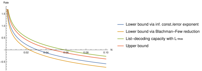
Figure 1: Comparison of different bounds for the $(N,L-1)$-list-decoding problem. The horizontal axis is $N$ and the vertical axis is the value of bounds. We plot bounds for $L=5$. Recall that the rate (Equation 1) of a multiple packing is defined as the (normalized) number of points per volume which can be negative. The expressions for all bounds can be found in Equations 2, 3, 4 and 5.

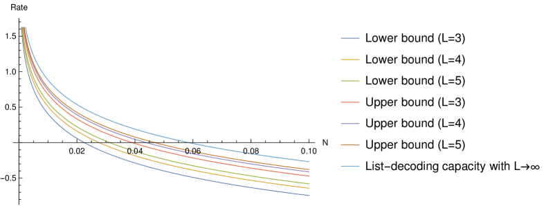
Figure 2: Plots of the best known lower bound (Equation 2) on $C_{L-1}(N)$ and the Elias–Bassalygo-type upper bound for $L=3,4,5$. As $L$ increases, they both converge from below to $C_{\mathrm{LD}}(N)$ (Equation 5). The lower bound Equation 2 derived in this paper is under the average-radius notion of multiple packing. Moreover, it can be obtained using a connection with error exponents [ZV22d] under the standard notion of multiple packing.

IV List-decoding capacity for large $L$

All bounds in this paper hold for any fixed $L$. In this section, we discuss the impact of our finite-$L$ bounds on the understanding of the limiting values of the largest multiple packing density as $L\to\infty$. Some of these results were known previously and others follow from the bounds in the current paper.

Characterizing $C_{L-1}(N)$ or $\overline{C}_{L-1}(N)$ is a difficult task that is out of reach given the current techniques. However, if the list-size $L$ is allowed to grow, we can actually characterize

$$C_{\mathrm{LD}}(N)\coloneqq\lim_{L\to\infty}C_{L-1}(N),\quad\overline{C}_{\mathrm{LD}}(N)\coloneqq\lim_{L\to\infty}\overline{C}_{L-1}(N),$$

where the subscript $\mathrm{LD}$ denotes List-Decoding.

The value of $C_{\mathrm{LD}}(N)$ is characterized in [ZV22b] which equals $\frac{1}{2}\ln\frac{1}{2\pi eN}$.

Theorem 1 ([ZV22b]).

Let $N>0$. Then for any $\varepsilon>0$,

1. There exist $(N,L-1)$-multiple packings of rate $\frac{1}{2}\ln\frac{1}{2\pi eN}-\varepsilon$ for some $L={\mathcal{O}}\left(\frac{1}{\varepsilon}\ln\frac{1}{\varepsilon}\right)$;

2. Any $(N,L-1)$-multiple packing of rate $\frac{1}{2}\ln\frac{1}{2\pi eN}+\varepsilon$ must satisfy $L=e^{\Omega(n\varepsilon)}$.

Therefore, $C_{\mathrm{LD}}(N)=\frac{1}{2}\ln\frac{1}{2\pi eN}$.

Moreover, we claim $\overline{C}_{\mathrm{LD}}(N)=\frac{1}{2}\ln\frac{1}{2\pi eN}$. For an upper bound, recall that average-radius list-decodability implies (regular) list-decodability. Therefore, any upper bound on $C_{L-1}(N)$ is also an upper bound on $\overline{C}_{L-1}(N)$. We already saw an upper bound on $C_{L-1}(N)$ in Equation 4 that approaches $\frac{1}{2}\ln\frac{1}{2\pi eN}$ as $L\to\infty$. Indeed, according to Theorem 8, for sufficiently large $L$, our construction achieves $\frac{1}{2}\ln\frac{1}{2\pi eN}$ under average-radius multiple packing.

Theorem 2.

For any $N>0$, $\overline{C}_{\mathrm{LD}}(N)=\frac{1}{2}\ln\frac{1}{2\pi eN}$.

V Our techniques

We summarize our techniques below.

To obtain lower bounds on the largest multiple packing density, our basic strategy is random coding with expurgation, a standard tool from information theory. To show the existence of a list-decodable code of rate $R$, we simply randomly sample $e^{nR}$ points independently each according to a certain distribution. There might be bad lists of size $L$ that violates the multiple packing condition. We then throw away (a.k.a. expurgate) one point from each of the bad lists. By carefully analyzing the error event and choosing a proper rate, we can guarantee that the remaining code has essentially the same rate after the removal process. We then get a list-decodable code of rate $R$ by noting that the remaining code contains no bad lists.

In the above framework, the key ingredient is a good estimate on the probability of the error event, i.e., the probability that the list-decoding radius of a size-$L$ list is smaller than $\sqrt{nN}$. Under the standard notion of multiple packing, the list-decoding radius is the Chebyshev radius of the list, i.e., the radius of the smallest ball containing the list. Under the average-radius notion of multiple packing, the (squared) list-decoding radius is the average squared radius of the list, i.e., the average squared distance from each point in the list to the centroid of the list.

Using the above idea, we first construct a finite codebook with minimum average squared radius $nN$ and supported over the hypercube $[-K,K]^{n}$ for a suitably chosen $K$. This is obtained by expurgating a random codebook obtained by choosing points independently and uniformly from $[-K,K]^{n}$. The finite codebook is then tiled across ${\mathbb{R}}^{n}$ to obtain an infinite constellation with the aforementioned density and minimum average squared radius $nN$. This construction is loosely inspired by the infinite constellations [Pol94] which was originally studied in the context of coding for the additive white Gaussian noise channel. A similar construction was used by [ZV22b] to derive lower bounds on $C_{\mathrm{LD}}(N)$ for large $L$.

The exact exponents of the probability of the error event are obtained using Cramér’s large deviation principle and the Laplace’s method.

As a technical contribution, we discover several new representations of the average radius and the Chebyshev radius. They play crucial roles in facilitating the analyses and the applications of some of these representations go beyond the scope of this paper. To name a few, the average squared radius of a list can be written as a quadratic form associated with the list. This representation is used to analyze Gaussian codes and spherical codes in [ZV22c] and infinite constellations in this paper. The average squared radius can also be written as the difference between the average (squared) norm of points in the list and the (squared) norm of the centroid of the list. This representation is used to analyze spherical codes and ball codes in [ZV22c]. The average squared radius can be further written as the average pairwise distance of the list. This allows us to give a one-line proof of the Blachman–Few reduction and its strengthened version [ZV22c]. Yet another way of writing the average squared radius using the average norm and the average pairwise correlation turns out to be useful for the proof of the Plotkin-type bound [ZV22c].

VI Organization of the paper

This paper derives a lower bound on the largest multiple packing density which turns out to be the best known so far. The rest of the paper is organized as follows. Notational conventions and preliminary definitions/facts are listed in Sections VII and VIII, respectively. After that, we present in Section IX the formal definitions of multiple packing and pertaining notions. We also discuss different notions of density of codes used in the literature. Furthermore, we obtain several novel representations of the Chebyshev radius and the average squared radius which are crucial for estimating their tail probabilities. In Section X, we formally introduce our construction and prove the main result. We end the paper with several open questions in Section XI.

VII Notation

Conventions. Sets are denoted by capital letters in calligraphic typeface, e.g., ${\mathcal{C}},{\mathcal{B}}$, etc. Random variables are denoted by lower case letters in boldface or capital letters in plain typeface, e.g., ${\mathbf{x}},S$, etc. Their realizations are denoted by corresponding lower case letters in plain typeface, e.g., $x,s$, etc. Vectors (random or fixed) of length $n$, where $n$ is the blocklength without further specification, are denoted by lower case letters with underlines, e.g., ${\underline{\mathbf{x}}},{\underline{\mathbf{g}}},{\underline{x}},{\underline{g}}$, etc. Vectors of length different from $n$ are denoted by an arrow on top and the length will be specified whenever used, e.g., $\vec{t},\vec{\alpha}$, etc. The $i$-th entry of a vector ${\underline{x}}\in{\mathcal{X}}^{n}$ is denoted by ${\underline{x}}(i)$ since we can alternatively think of ${\underline{x}}$ as a function from $[n]$ to ${\mathcal{X}}$. Same for a random vector ${\underline{\mathbf{x}}}$. Matrices are denoted by capital letters, e.g., $A,\Sigma$, etc. Similarly, the $(i,j)$-th entry of a matrix $G\in{\mathbb{F}}^{n\times m}$ is denoted by $G(i,j)$. We sometimes write $G_{n\times m}$ to explicitly specify its dimension. For square matrices, we write $G_{n}$ for short. Letter $I$ is reserved for identity matrix.

Functions. We use the standard Bachmann–Landau (Big-Oh) notation for asymptotics of real-valued functions in positive integers.

For two real-valued functions $f(n),g(n)$ of positive integers, we say that $f(n)$ asymptotically equals $g(n)$, denoted $f(n)\asymp g(n)$, if

$$\lim_{n\to\infty}\frac{f(n)}{g(n)}=1.$$

For instance, $2^{n+\log n}\asymp 2^{n+\log n}+2^{n}$, $2^{n+\log n}\not\asymp 2^{n}$. We write $f(n)\doteq g(n)$ (read $f(n)$ dot equals $g(n)$) if the coefficients of the dominant terms in the exponents of $f(n)$ and $g(n)$ match,

$$\lim_{n\to\infty}\frac{\log f(n)}{\log g(n)}=1.$$

For instance, $2^{3n}\doteq 2^{3n+n^{1/4}}$, $2^{2^{n}}\not\doteq 2^{2^{n+\log n}}$. Note that $f(n)\asymp g(n)$ implies $f(n)\doteq g(n)$, but the converse is not true.

For any $q\in{\mathbb{R}}_{>0}$, we write $\log_{q}(\cdot)$ for the logarithm to the base $q$. In particular, let $\log(\cdot)$ and $\ln(\cdot)$ denote logarithms to the base $2$ and $e$, respectively.

For any ${\mathcal{A}}\subseteq\Omega$, the indicator function of ${\mathcal{A}}$ is defined as, for any $x\in\Omega$,

$$\mathds{1}_{{\mathcal{A}}}(x)\coloneqq\begin{cases}1,&x\in{\mathcal{A}}\\ 0,&x\notin{\mathcal{A}}\end{cases}.$$

At times, we will slightly abuse notation by saying that $\mathds{1}_{{\mathsf{A}}}$ is $1$ when event ${\mathsf{A}}$ happens and 0 otherwise. Note that $\mathds{1}_{{\mathcal{A}}}(\cdot)=\mathds{1}{\left\{\cdot\in{\mathcal{A}}\right\}}$.

Sets. For any two nonempty sets ${\mathcal{A}}$ and ${\mathcal{B}}$ with addition and multiplication by a real scalar, let ${\mathcal{A}}+{\mathcal{B}}$ denote the Minkowski sum of them which is defined as ${\mathcal{A}}+{\mathcal{B}}\coloneqq\left\{a+b\colon a\in{\mathcal{A}},b\in{\mathcal{B}}\right\}$. If ${\mathcal{A}}=\{x\}$ is a singleton set, we write $x+{\mathcal{B}}$ and for $\{x\}+{\mathcal{B}}$. For any $r\in{\mathbb{R}}$, the $r$-dilation of ${\mathcal{A}}$ is defined as $r{\mathcal{A}}\coloneqq\left\{r{\underline{a}}:{\underline{a}}\in{\mathcal{A}}\right\}$. In particular, $-{\mathcal{A}}\coloneqq(-1){\mathcal{A}}$.

For $M\in{\mathbb{Z}}_{>0}$, we let $[M]$ denote the set of first $M$ positive integers $\{1,2,\cdots,M\}$.

Geometry. Let $\left\|\cdot\right\|_{2}$ denote the Euclidean/$\ell_{2}$-norm. Specifically, for any ${\underline{x}}\in{\mathbb{R}}^{n}$,

$$\left\|{\underline{x}}\right\|_{2}\coloneqq\left(\sum_{i=1}^{n}{\underline{x}}(i)^{2}\right)^{1/2}.$$

With slight abuse of notation, we let $|\cdot|$ denote the “volume” of a set w.r.t. a measure that is obvious from the context. If ${\mathcal{A}}$ is a finite set, then $|{\mathcal{A}}|$ denotes the cardinality of ${\mathcal{A}}$ w.r.t. the counting measure. For a set ${\mathcal{A}}\subset{\mathbb{R}}^{n}$, let

$$\operatorname{aff}({\mathcal{A}}) \coloneqq\left\{\sum_{i=1}^{k}\lambda_{i}{\underline{a}}_{i}:k\in{\mathbb{Z}}_{\geq 1};\;\forall i\in[k],{\underline{a}}_{i}\in{\mathcal{A}},\lambda_{i}\in{\mathbb{R}},\sum_{i=1}^{k}\lambda_{i}=1\right\}$$

denote the affine hull of ${\mathcal{A}}$, i.e., the smallest affine subspace containing ${\mathcal{A}}$. If ${\mathcal{A}}$ is a connected compact set in ${\mathbb{R}}^{n}$ with nonempty interior and $\operatorname{aff}({\mathcal{A}})={\mathbb{R}}^{n}$, then $|{\mathcal{A}}|$ denotes the volume of ${\mathcal{A}}$ w.r.t. the $n$-dimensional Lebesgue measure. If $\operatorname{aff}({\mathcal{A}})$ is a $k$-dimensional affine subspace for $1\leq k<n$, then $|{\mathcal{A}}|$ denotes the $k$-dimensional Lebesgue volume of ${\mathcal{A}}$.

The closed $n$-dimensional Euclidean unit ball is defined as

$${\mathcal{B}}^{n}\coloneqq\left\{{\underline{y}}\in{\mathbb{R}}^{n}\colon\left\|{\underline{y}}\right\|_{2}\leq 1\right\}.$$

The $(n-1)$-dimensional Euclidean unit sphere is defined as

$${\mathcal{S}}^{n-1}\coloneqq\left\{{\underline{y}}\in{\mathbb{R}}^{n}\colon\left\|{\underline{y}}\right\|_{2}=1\right\}.$$

For any ${\underline{x}}\in{\mathbb{R}}^{n}$ and $r\in{\mathbb{R}}_{>0}$, let ${\mathcal{B}}^{n}(r)\coloneqq r{\mathcal{B}}^{n},{\mathcal{S}}^{n-1}(r)\coloneqq r{\mathcal{S}}^{n-1}$ and ${\mathcal{B}}^{n}({\underline{x}},r)\coloneqq{\underline{x}}+r{\mathcal{B}}^{n},{\mathcal{S}}^{n-1}({\underline{x}},r)\coloneqq{\underline{x}}+r{\mathcal{S}}^{n-1}$.

Let $V_{n}\coloneqq|{\mathcal{B}}^{n}|$.

VIII Preliminaries

Lemma 3 (Change of variable).

Let ${\mathcal{U}}\subset{\mathbb{R}}^{n}$ be an open set and $\varphi\colon{\mathcal{U}}\to{\mathbb{R}}^{n}$ be an injective differentiable function with continuous partial derivatives, the Jacobian of which is nonzero for every ${\underline{x}}\in{\mathcal{U}}$. Then for any compactly supported, continuous function $f\colon\varphi({\mathcal{U}})\to{\mathbb{R}}$, the substitution ${\underline{v}}=\varphi({\underline{u}})$ yields the following formula

$$\int_{\varphi({\mathcal{U}})}f({\underline{v}})\mathrm{d}{\underline{v}} =\int_{\mathcal{U}}f(\varphi({\underline{u}}))\left|\det(\nabla\varphi)({\underline{u}})\right|\mathrm{d}{\underline{u}},$$

where $\nabla\varphi\in{\mathbb{R}}^{n\times n}$ denotes the Jacobian matrix of $\varphi$.

Theorem 4 (Laplace’s method).

Suppose $f\colon{\mathbb{R}}^{d}\to{\mathbb{R}}$ is a twice continuously differentiable function on ${\mathcal{A}}\subset{\mathbb{R}}^{d}$, and there exists a unique point $\vec{t}^{*}\in\operatorname{int}({\mathcal{A}})$ (where $\operatorname{int}(\cdot)$ denotes the interior of a set) such that

$$f(\vec{t}^{*})=\min_{\vec{t}\in{\mathcal{A}}}f(\vec{t}),\quad(\operatorname{Hess}f)(\vec{t}^{*})\succ 0,$$

where $\operatorname{Hess}f\in{\mathbb{R}}^{d\times d}$ denotes the Hessian matrix of $f$. Suppose $g(\vec{t})$ is positive. Then

$$\int_{{\mathcal{A}}}g(\vec{t})e^{-Mf(\vec{t})}\mathrm{d}\vec{t} \stackrel{{\scriptstyle M\to\infty}}{{\asymp}}e^{-Mf(\vec{t}^{*})}\left(\frac{2\pi}{M}\right)^{d/2}\frac{g(\vec{t}^{*})}{\sqrt{\det((\operatorname{Hess}f)(\vec{t}^{*}))}}.$$

Theorem 5 (Cramér).

Let $\left\{{\mathbf{x}}_{i}\right\}_{i=1}^{n}$ be a sequence of i.i.d. real-valued random variables. Let ${\mathbf{s}}_{n}\coloneq\frac{1}{n}\sum_{i=1}^{n}{\mathbf{x}}_{i}$. Then for any closed ${\mathcal{F}}\subset{\mathbb{R}}$,

$$\limsup_{n\to\infty}\frac{1}{n}\ln\Pr\left[{\mathbf{s}}_{n}\in{\mathcal{F}}\right] \leq-\inf_{x\in{\mathcal{F}}}\sup_{\lambda\in{\mathbb{R}}}\left\{\lambda x-\ln\mathbb{E}\left[e^{\lambda{\mathbf{x}}_{1}}\right]\right\};$$

and for any open ${\mathcal{G}}\subset{\mathbb{R}}$,

$$\liminf_{n\to\infty}\frac{1}{n}\ln\Pr\left[{\mathbf{s}}_{n}\in{\mathcal{G}}\right] \geq-\inf_{x\in{\mathcal{G}}}\sup_{\lambda\in{\mathbb{R}}}\left\{\lambda x-\ln\mathbb{E}\left[e^{\lambda{\mathbf{x}}_{1}}\right]\right\}.$$

Furthermore, when ${\mathcal{F}}$ or ${\mathcal{G}}$ corresponds to the upper (resp. lower) tail of ${\mathbf{s}}_{n}$, the maximizer $\lambda\geq 0$ (resp. $\lambda\leq 0$).

IX Basic definitions and facts

Given the intimate connection between packing and error-correcting codes, we will interchangeably use the terms “multiple packing” and “list-decodable code”. The parameter $L\in{\mathbb{Z}}_{\geq 2}$ is called the multiplicity of overlap or the list-size. The parameter $N$ is called the noise power constraints. Elements of a packing are called either points or codewords. We will call a size-$L$ subset of a packing an $L$-list. This paper is only concerned with the fundamental limits of multiple packing for asymptotically large dimension $n\to\infty$. When we say “a” code ${\mathcal{C}}$, we always mean an infinite sequence of codes $\left\{{\mathcal{C}}_{i}\right\}_{i\geq 1}$ where ${\mathcal{C}}_{i}\subset{\mathbb{R}}^{n_{i}}$ and $\left\{n_{i}\right\}_{i\geq 1}$ is an increasing sequence of positive integers.

In the rest of this section, we list a sequence of formal definitions and some facts associated with these definitions.

Definition 1 (Multiple packing).

Let $N>0$ and $L\in{\mathbb{Z}}_{\geq 2}$. A subset ${\mathcal{C}}\subseteq{\mathbb{R}}^{n}$ is called a $(N,L-1)$-list-decodable code (a.k.a. an $(N,L-1)$-multiple packing) if for every ${\underline{y}}\in{\mathbb{R}}^{n}$,

$$\left|{\mathcal{C}}\cap{\mathcal{B}}^{n}({\underline{y}},\sqrt{nN})\right|\leq L-1.$$ (6)

The rate (a.k.a. density) of ${\mathcal{C}}$ is defined as

$$R({\mathcal{C}})\coloneqq \limsup_{K\to\infty}\frac{1}{n}\ln\frac{\left|{\mathcal{C}}\cap(K{\mathcal{B}})\right|}{\left|K{\mathcal{B}}\right|},$$ (7)

where ${\mathcal{B}}$ is an arbitrary centrally symmetric connected compact set in ${\mathbb{R}}^{n}$ with nonempty interior.

Remark 1.

Common choices of ${\mathcal{B}}$ include the unit ball ${\mathcal{B}}^{n}$, the unit cube $[-1,1]^{n}$, the fundamental Voronoi region ${\mathcal{V}}_{\Lambda}$ of a (full-rank) lattice $\Lambda\subset{\mathbb{R}}^{n}$, etc. Some choices of ${\mathcal{B}}$ may be more convenient than the others for analyzing certain ensembles of packings. Therefore, we do not fix the choice of ${\mathcal{B}}$ in Definition 1.

Remark 2.

The rate of a packing (as per Equation 7) is also called the normalized logarithmic density in the literature. It measures the the normalized number of points per unit volume.

Note that the condition given by Equation 6 is equivalent to that for any $({\underline{x}}_{1},\cdots,{\underline{x}}_{L})\in\binom{{\mathcal{C}}}{L}$,

$$\bigcap_{i=1}^{L}{\mathcal{B}}^{n}({\underline{x}}_{i},\sqrt{nN})=\emptyset.$$ (8)

Definition 2 (Chebyshev radius and average squared radius of a list).

Let ${\underline{x}}_{1},\cdots,{\underline{x}}_{L}$ be $L$ points in ${\mathbb{R}}^{n}$. Then the squared Chebyshev radius $\operatorname{rad}^{2}({\underline{x}}_{1},\cdots,{\underline{x}}_{L})$ of ${\underline{x}}_{1},\cdots,{\underline{x}}_{L}$ is defined as the (squared) radius of the smallest ball containing ${\underline{x}}_{1},\cdots,{\underline{x}}_{L}$, i.e.,

$$\operatorname{rad}^{2}({\underline{x}}_{1},\cdots,{\underline{x}}_{L})\coloneqq \min_{{\underline{y}}\in{\mathbb{R}}^{n}}\max_{i\in[L]}\left\|{\underline{x}}_{i}-{\underline{y}}\right\|_{2}^{2}.$$ (9)

The average squared radius $\overline{\operatorname{rad}}^{2}({\underline{x}}_{1},\cdots,{\underline{x}}_{L})$ of ${\underline{x}}_{1},\cdots,{\underline{x}}_{L}$ is defined as the average squared distance to the centroid, i.e.,

$$\overline{\operatorname{rad}}^{2}({\underline{x}}_{1},\cdots,{\underline{x}}_{L})\coloneqq \frac{1}{L}\sum_{i=1}^{L}{\left\|{\underline{x}}_{i}-{\underline{x}}\right\|_{2}^{2}},$$ (10)

where ${\underline{x}}\coloneqq\frac{1}{L}\sum_{i=1}^{L}{\underline{x}}_{i}$ is the centroid of ${\underline{x}}_{1},\cdots,{\underline{x}}_{L}$. We refer to the square root of the average squared radius as the average radius of the list.

Remark 3.

One should note that for an $L$-list ${\mathcal{L}}$ of points, the smallest ball containing ${\mathcal{L}}$ is not necessarily the same as the circumscribed ball, i.e., the ball such that all points in ${\mathcal{L}}$ live on the boundary of the ball. The circumscribed ball of the polytope $\operatorname{conv}\left\{{\mathcal{L}}\right\}$ spanned by the points in ${\mathcal{L}}$ may not exist. If it does exist, it is not necessarily the smallest one containing ${\mathcal{L}}$. However, whenever it exists, the smallest ball containing ${\mathcal{L}}$ must be the circumscribed ball of a certain subset of ${\mathcal{L}}$.

Remark 4.

We remark that the motivation behind the definition of average squared radius (Equation 10) is to replace the maximization in Equation 9 with average.

$$\min_{{\underline{y}}\in{\mathbb{R}}^{n}}\mathop{\mathbb{E}}_{{\mathbf{i}}\sim[L]}\left[\left\|{\underline{x}}_{\mathbf{i}}-{\underline{y}}\right\|_{2}^{2}\right] =\min_{{\underline{y}}\in{\mathbb{R}}^{n}}\frac{1}{L}\sum_{i=1}^{L}\sum_{j=1}^{n}\left({\underline{x}}_{i}(j)-{\underline{y}}(j)\right)^{2}$$

$$=\min_{(y_{1},\cdots,y_{n})\in{\mathbb{R}}^{n}}\sum_{j=1}^{n}\frac{1}{L}\sum_{i=1}^{L}\left({\underline{x}}_{i}(j)-y_{j}\right)^{2}$$ (11)

$$=\sum_{j=1}^{n}\min_{y_{j}\in{\mathbb{R}}}\frac{1}{L}\sum_{i=1}^{L}\left({\underline{x}}_{i}(j)-y_{j}\right)^{2}$$ (12)

$$=\frac{1}{L}\sum_{i=1}^{L}\sum_{j=1}^{n}\left({\underline{x}}_{i}(j)-y_{j}^{*}\right)^{2}$$ (13)

$$=\frac{1}{L}\sum_{i=1}^{L}\left\|{\underline{x}}_{i}-{\underline{x}}\right\|_{2}^{2}.$$ (14)

Equation 12 holds since the inner summation $\frac{1}{L}\sum_{i=1}^{L}\left({\underline{x}}_{i}(j)-{\underline{y}}(j)\right)^{2}$ in Equation 11 only depends on $y_{j}$ among all $y_{1},\cdots,y_{n}$. Equation 13 follows since for each $j$, the minimizer of the minimization in Equation 12 is $y_{j}^{*}\coloneqq\frac{1}{L}\sum_{i=1}^{L}{\underline{x}}_{i}(j)$. In Equation 14, the minimizer ${\underline{y}}^{*}$ equals ${\underline{x}}\coloneqq\frac{1}{L}\sum_{i=1}^{L}{\underline{x}}_{i}$.

Definition 3 (Chebyshev radius and average squared radius of a code).

Given a code ${\mathcal{C}}\subset{\mathbb{R}}^{n}$ of rate $R$, the squared $(L-1)$-list-decoding radius of ${\mathcal{C}}$ is defined as

$$\operatorname{rad}^{2}_{L}({\mathcal{C}})\coloneqq \min_{{\mathcal{L}}\in\binom{{\mathcal{C}}}{L}}\operatorname{rad}^{2}({\mathcal{L}}).$$ (15)

The $(L-1)$-average squared radius of ${\mathcal{C}}$ is defined as

$$\overline{\operatorname{rad}}^{2}_{L}({\mathcal{C}})\coloneqq \min_{{\mathcal{L}}\in\binom{{\mathcal{C}}}{L}}\overline{\operatorname{rad}}^{2}({\mathcal{L}}).$$ (16)

Definition 4 (Average-radius multiple packing).

A subset ${\mathcal{C}}\subset{\mathbb{R}}^{n}$ is called an $(N,L-1)$-average-radius list-decodable code (a.k.a. an $(N,L-1)$-average-radius multiple packing) if $\overline{\operatorname{rad}}^{2}_{L}({\mathcal{C}})>nN$. The rate (a.k.a. density) $R({\mathcal{C}})$ of ${\mathcal{C}}$ is given by Equation 7. The $(N,L-1)$-average-radius list-decoding capacity (a.k.a. $(N,L-1)$ average-radius multiple packing density) is defined as

$$\overline{C}_{L-1}(N)\coloneqq\limsup_{n\to\infty}\limsup_{{\mathcal{C}}\subseteq{\mathbb{R}}^{n}\colon\overline{\operatorname{rad}}^{2}_{L}({\mathcal{C}})>nN}R({\mathcal{C}}).$$

The squared $(L-1)$-average-radius list-decoding radius at rate $R$ (without input constraint) is defined as

$$\overline{\operatorname{rad}}^{2}_{L}(R)\coloneqq \limsup_{n\to\infty}\limsup_{{\mathcal{C}}\subseteq{\mathbb{R}}^{n}\colon R({\mathcal{C}})\geq R}\overline{\operatorname{rad}}^{2}_{L}({\mathcal{C}}).$$

Note that $(L-1)$-list-decodability defined by Equation 8 is equivalent to $\operatorname{rad}^{2}_{L}({\mathcal{C}})>nN$. We also define the $(N,L-1)$-list-decoding capacity (a.k.a. $(N,L-1)$-multiple packing density) $C_{L-1}(N)$ and the $(L-1)$-list-decoding radius $\operatorname{rad}^{2}_{L}(R)$ at rate $R$:

$$C_{L-1}(N) \coloneqq\limsup_{n\to\infty}\limsup_{{\mathcal{C}}\subseteq{\mathbb{R}}^{n}\colon\operatorname{rad}^{2}_{L}({\mathcal{C}})>nN}R({\mathcal{C}}),$$

$$\operatorname{rad}^{2}_{L}(R) \coloneqq\limsup_{n\to\infty}\limsup_{{\mathcal{C}}\subseteq{\mathbb{R}}^{n}\colon R({\mathcal{C}})\geq R}\operatorname{rad}^{2}_{L}({\mathcal{C}}).$$

Since the average radius is at most the Chebyshev radius, average-radius list-decodability is stronger than regular list-decodability. Any lower (resp. upper) bound on $\overline{C}_{L-1}(N)$ (resp. $C_{L-1}(N)$) is automatically a lower (resp. upper) bound on $C_{L-1}(N)$ (resp. $\overline{C}_{L-1}(N)$). Proving upper/lower bounds on $C_{L-1}(N)$ (resp. $\overline{C}_{L-1}(N)$) is equivalent to proving upper/lower bounds on $\operatorname{rad}^{2}_{L}(R)$ (resp. $\overline{\operatorname{rad}}^{2}_{L}(R)$).

IX-A Different notions of density of packings

We measure the density of a packing using Equation 7. In the literature, there exists another commonly used notion of density for multiple packings. It counts the fraction of space occupied by the union of the balls of radius $\sqrt{nN}$ centered around points in the packing. Specifically, for an $(N,L-1)$-packing ${\mathcal{C}}\subset{\mathbb{R}}^{n}$,

$$\Delta({\mathcal{C}})\coloneqq \limsup_{P\to\infty}\frac{1}{n}\ln\left(\left|\bigcup_{{\underline{x}}\in{\mathcal{C}}}{\mathcal{B}}^{n}({\underline{x}},\sqrt{nN})\cap{\mathcal{B}}^{n}(\sqrt{nP})\right|\big{/}\left|{\mathcal{B}}^{n}(\sqrt{nP})\right|\right).$$ (17)

We prove the following statement.

Theorem 6.

Let $N>0$ and $L\in{\mathbb{Z}}_{\geq 2}$. Let ${\mathcal{C}}\subset{\mathbb{R}}^{n}$ be an $(N,L-1)$-multiple packing. Then $\Delta({\mathcal{C}})\stackrel{{\scriptstyle n\to\infty}}{{\asymp}}R({\mathcal{C}})+\frac{1}{2}\ln(2\pi eN)$.

Proof.

Note that for sufficiently large $P$,

$$\left|\bigcup_{{\underline{x}}\in{\mathcal{C}}}{\mathcal{B}}^{n}({\underline{x}},\sqrt{nN})\cap{\mathcal{B}}^{n}(\sqrt{nP})\right| \lesssim\left|{\mathcal{C}}\cap{\mathcal{B}}^{n}(\sqrt{nP})\right|\cdot\left|{\mathcal{B}}^{n}(\sqrt{nN})\right|.$$

Therefore,

$$\Delta({\mathcal{C}}) \leq\limsup_{P\to\infty}\frac{1}{n}\ln\frac{\left|{\mathcal{C}}\cap{\mathcal{B}}^{n}(\sqrt{nP})\right|\cdot\left|{\mathcal{B}}^{n}(\sqrt{nN})\right|}{\left|{\mathcal{B}}^{n}(\sqrt{nP})\right|}$$

$$=R({\mathcal{C}})+\frac{1}{n}\ln\left|{\mathcal{B}}^{n}(\sqrt{nN})\right|$$

$$\asymp R({\mathcal{C}})+\frac{1}{n}\ln\left(\sqrt{nN}^{n}\cdot\frac{1}{\sqrt{\pi n}}\sqrt{\frac{2\pi e}{n}}^{n}\right)$$

$$\asymp R({\mathcal{C}})+\frac{1}{2}\ln(2\pi eN).$$ (18)

On the other hand, we claim that for sufficiently large $P$,

$$\left|\bigcup_{{\underline{x}}\in{\mathcal{C}}}{\mathcal{B}}^{n}({\underline{x}},\sqrt{nN})\cap{\mathcal{B}}^{n}(\sqrt{nP})\right| \gtrsim\frac{1}{L-1}\left|{\mathcal{C}}\cap{\mathcal{B}}^{n}(\sqrt{nP})\right|\cdot\left|{\mathcal{B}}^{n}(\sqrt{nN})\right|.$$ (19)

The above claim is justified at the end of this subsection. Then following the same lines of calculations above, we have

$$\Delta({\mathcal{C}}) \geq R({\mathcal{C}})+\frac{1}{2}\ln(2\pi eN)-o(1).$$ (20)

Combining Equations 18 and 20, we have that for any $(N,L-1)$-packing ${\mathcal{C}}$,

$$\Delta({\mathcal{C}}) \asymp R({\mathcal{C}})+\frac{1}{2}\ln(2\pi eN).$$

To see Equation 19, consider the set of convex sets

$${\mathscr{D}} \coloneqq\left\{{\mathcal{D}}({\underline{x}}):{\underline{x}}\in{\mathcal{C}},\;{\mathcal{B}}^{n}({\underline{x}},\sqrt{nN})\cap{\mathcal{B}}^{n}(\sqrt{nP})\neq\emptyset\right\},$$

where

$${\mathcal{D}}({\underline{x}}) \coloneqq{\mathcal{B}}^{n}({\underline{x}},\sqrt{nN})\cap{\mathcal{B}}^{n}(\sqrt{nP}).$$

Note that some elements in ${\mathscr{D}}$ are balls ${\mathcal{B}}^{n}({\underline{x}},\sqrt{nN})$, while other elements are the intersection of two balls ${\mathcal{B}}^{n}({\underline{x}},\sqrt{nN})\cap{\mathcal{B}}^{n}(\sqrt{nP})$ for some ${\underline{x}}\in{\mathcal{C}}$.

We now rearrange all ${\mathcal{D}}({\underline{x}})$ in ${\mathscr{D}}$ so that they become disjoint. Then the volume induced by the resulting packing is

$$\sum_{{\mathcal{D}}\in{\mathscr{D}}}\left|{\mathcal{D}}\right| =\sum_{\begin{subarray}{c}{\underline{x}}\in{\mathcal{C}}\\ {\mathcal{B}}^{n}({\underline{x}},\sqrt{nN})\cap{\mathcal{B}}^{n}(\sqrt{nP})\neq\emptyset\end{subarray}}|{\mathcal{D}}({\underline{x}})|$$

$$\approx\sum_{{\underline{x}}\in{\mathcal{C}}\cap{\mathcal{B}}^{n}(\sqrt{nP})}\left|{\mathcal{D}}({\underline{x}})\right|$$

$$=\sum_{{\underline{x}}\in{\mathcal{C}}\cap{\mathcal{B}}^{n}(\sqrt{nP})}\left|{\mathcal{B}}^{n}({\underline{x}},\sqrt{nN})\cap{\mathcal{B}}^{n}(\sqrt{nP})\right|.$$ (21)

On the other hand, for any ${\underline{y}}\in\bigcup\limits_{{\mathcal{D}}\in{\mathscr{D}}}{\mathcal{D}}$, it can split into at most $L-1$ points after the above process since by $(L-1)$-list-decodability, each point in a ball is covered by at most $L-2$ other balls. Therefore, the volume induced by the rearranged packing is at most

$$(L-1)\left|\bigcup_{{\mathcal{D}}\in{\mathscr{D}}}{\mathcal{D}}\right| =(L-1)\left|\bigcup_{{\underline{x}}\in{\mathcal{C}}}{\mathcal{B}}^{n}({\underline{x}},\sqrt{nN})\cap{\mathcal{B}}^{n}(\sqrt{nP})\right|.$$ (22)

Combining Equations 21 and 22, we have, for sufficiently large $P$,

$$\left|\bigcup_{{\underline{x}}\in{\mathcal{C}}}{\mathcal{B}}^{n}({\underline{x}},\sqrt{nN})\cap{\mathcal{B}}^{n}(\sqrt{nP})\right| \gtrsim\frac{1}{L-1}\sum_{{\underline{x}}\in{\mathcal{C}}\cap{\mathcal{B}}^{n}(\sqrt{nP})}\left|{\mathcal{B}}^{n}({\underline{x}},\sqrt{nN})\cap{\mathcal{B}}^{n}(\sqrt{nP})\right|$$

$$\approx\frac{1}{L-1}\left|{\mathcal{C}}\cap{\mathcal{B}}^{n}(\sqrt{nP})\right|\left|{\mathcal{B}}^{n}(\sqrt{nN})\right|,$$

as claimed in Equation 19. ∎

IX-B Chebyshev radius and average radius

In this section, we present several different representations of the Chebyshev radius and average squared radius. Some of them will be crucially used in the subsequent sections of this paper. These representations are summarized in the following theorem which will be proved in the subsequent subsections.

Theorem 7.

Let $L\in{\mathbb{Z}}_{\geq 2}$ and ${\underline{x}}_{1},\cdots,{\underline{x}}_{L}\in{\mathbb{R}}^{n}$. Then the squared Chebyshev radius of ${\underline{x}}_{1},\cdots,{\underline{x}}_{L}$ admits the following alternative representations:

1. $\begin{aligned} \operatorname{rad}^{2}({\underline{x}}_{1},\cdots,{\underline{x}}_{L})&=\max_{{\vec{z}}\in\Delta_{L}}\sum_{i=1}^{L}{\vec{z}}(i)\left\|{\underline{x}}_{i}-{\underline{y}}_{\vec{z}}\right\|_{2}^{2},\end{aligned}$ where ${\underline{y}}_{\vec{z}}\coloneqq\sum_{i=1}^{L}{\vec{z}}(i){\underline{x}}_{i}$ and $\Delta_{L}$ denotes the probability simplex on $[L]$;

2. $\begin{aligned} \operatorname{rad}^{2}({\underline{x}}_{1},\cdots,{\underline{x}}_{L})&=\lim_{p\to\infty}\operatorname{rad}^{(p)}({\underline{x}}_{1},\cdots,{\underline{x}}_{L}),\end{aligned}$ where

   $$\operatorname{rad}^{(p)}({\underline{x}}_{1},\cdots,{\underline{x}}_{L}) \coloneqq\left(\min_{{\underline{y}}\in{\mathbb{R}}^{n}}\frac{1}{L}\sum_{i=1}^{L}\left\|{\underline{x}}_{i}-{\underline{y}}\right\|_{2}^{2p}\right)^{1/p};$$

3. there exists a unique $1\leq q\leq\infty$ depending on ${\underline{x}}_{1},\cdots,{\underline{x}}_{L}$ such that

   $$\operatorname{rad}^{2}({\underline{x}}_{1},\cdots,{\underline{x}}_{L}) =\left(\frac{1}{L}\sum_{i=1}^{L}\left\|{\underline{x}}_{i}-{\underline{x}}\right\|_{2}^{2q}\right)^{1/q},$$

   and ${\underline{x}}\coloneqq\frac{1}{L}\sum_{i=1}^{L}{\underline{x}}_{i}$.

The average squared radius of ${\underline{x}}_{1},\cdots,{\underline{x}}_{L}$ admits the following alternative representations:

1. $\begin{aligned} \overline{\operatorname{rad}}^{2}({\underline{x}}_{1},\cdots,{\underline{x}}_{L})&=\frac{1}{L}\sum_{i=1}^{L}\left\|{\underline{x}}_{i}\right\|_{2}^{2}-\left\|{\underline{x}}\right\|_{2}^{2};\end{aligned}$

2. $\begin{aligned} \overline{\operatorname{rad}}^{2}({\underline{x}}_{1},\cdots,{\underline{x}}_{L})&=\frac{L-1}{L^{2}}\sum_{i=1}^{L}\left\|{\underline{x}}_{i}\right\|_{2}^{2}-\frac{1}{L^{2}}\sum_{(i,j)\in[L]^{2}:i\neq j}\left\langle{\underline{x}}_{i},{\underline{x}}_{j}\right\rangle;\end{aligned}$

3. $\begin{aligned} \overline{\operatorname{rad}}^{2}({\underline{x}}_{1},\cdots,{\underline{x}}_{L})&=\frac{1}{2L^{2}}\sum_{(i,j)\in[L]^{2}:i\neq j}\left\|{\underline{x}}_{i}-{\underline{x}}_{j}\right\|_{2}^{2}.\end{aligned}$

IX-B1 Another representation of the Chebyshev radius

The Chebyshev radius involves a minimax expression which is in general tricky to handle. One can use minimax theorem to interchange the min and max and then compute the inner min explicitly.

$$\operatorname{rad}^{2}({\underline{x}}_{1},\cdots,{\underline{x}}_{L}) =\min_{{\underline{y}}\in{\mathbb{R}}^{n}}\max_{i\in[L]}\left\|{\underline{x}}_{i}-{\underline{y}}\right\|_{2}^{2}=\min_{{\underline{y}}\in{\mathbb{R}}^{n}}\max_{{\vec{z}}\in\Delta_{L}}\sum_{i=1}^{L}{\vec{z}}(i)\left\|{\underline{x}}_{i}-{\underline{y}}\right\|_{2}^{2}.$$

The last equality follows since the maximum is always achieved by a singleton ${\vec{z}}\in\{0,1\}^{L}$. Note that the objective function on the RHS is linear (hence concave) in ${\vec{z}}$ and quadratic (hence convex) in ${\underline{y}}$. Therefore the max and min can be interchanged and we get

$$\max_{{\vec{z}}\in\Delta_{L}}\min_{{\underline{y}}\in{\mathbb{R}}^{n}}\sum_{i=1}^{L}{\vec{z}}(i)\left\|{\underline{x}}_{i}-{\underline{y}}\right\|_{2}^{2}=\max_{{\vec{z}}\in\Delta_{L}}\min_{{\underline{y}}\in{\mathbb{R}}^{n}}\sum_{j=1}^{n}\sum_{i=1}^{L}{\vec{z}}(i)\left({\underline{x}}_{i}(j)-{\underline{y}}(j)\right)^{2}=\max_{{\vec{z}}\in\Delta_{L}}\sum_{j=1}^{n}\min_{y_{j}\in{\mathbb{R}}}\sum_{i=1}^{L}{\vec{z}}(i)\left({\underline{x}}_{i}(j)-y_{j}\right)^{2}.$$

The last equality follows since each inner summation $\sum_{i=1}^{L}{\vec{z}}(i)\left({\underline{x}}_{i}(j)-{\underline{y}}(j)\right)^{2}$ only depends on ${\underline{y}}(j)$ among all ${\underline{y}}(1),\cdots,{\underline{y}}(n)$. For each $j$, the minimizing $y_{j}^{*}$ equals

$$y_{j}^{*} \coloneqq\frac{\sum_{i=1}^{L}{\vec{z}}(i){\underline{x}}_{i}(j)}{\sum_{i=1}^{L}{\vec{z}}(i)}=\sum_{i=1}^{L}{\vec{z}}(i){\underline{x}}_{i}(j),$$

where the last equality is because ${\vec{z}}\in\Delta_{L}$. Therefore

$$\operatorname{rad}^{2}({\underline{x}}_{1},\cdots,{\underline{x}}_{L}) =\max_{{\vec{z}}\in\Delta_{L}}\sum_{i=1}^{L}{\vec{z}}(i)\left\|{\underline{x}}_{i}-{\underline{y}}_{\vec{z}}\right\|_{2}^{2},$$ (23)

where ${\underline{y}}_{\vec{z}}\coloneqq\sum_{i=1}^{L}{\vec{z}}(i){\underline{x}}_{i}$.

IX-B2 Higher-order approximations to the Chebyshev radius

As explained in Remark 4, the average squared radius is a linear relaxation of the squared Chebyshev radius:

$$\overline{\operatorname{rad}}^{2}({\underline{x}}_{1},\cdots,{\underline{x}}_{L}) =\min_{{\underline{y}}\in{\mathbb{R}}^{n}}\mathop{\mathbb{E}}_{{\mathbf{i}}\sim[L]}\left[\left\|{\underline{x}}_{\mathbf{i}}-{\underline{y}}\right\|_{2}^{2}\right].$$ (24)

One may obtain better and better approximations to the squared Chebyshev radius by taking higher and higher order relaxations:

$$\operatorname{rad}^{(p)}({\underline{x}}_{1},\cdots,{\underline{x}}_{L}) =\min_{{\underline{y}}\in{\mathbb{R}}^{n}}\left(\mathop{\mathbb{E}}_{{\mathbf{i}}\sim[L]}\left[\left\|{\underline{x}}_{\mathbf{i}}-{\underline{y}}\right\|_{2}^{2p}\right]\right)^{1/p}=\left(\min_{{\underline{y}}\in{\mathbb{R}}^{n}}\mathop{\mathbb{E}}_{{\mathbf{i}}\sim[L]}\left[\left\|{\underline{x}}_{\mathbf{i}}-{\underline{y}}\right\|_{2}^{2p}\right]\right)^{1/p},$$ (25)

where $p\geq 1$. The second equality in Equation 25 follows since the $f(\cdot)=(\cdot)^{1/p}$ is monotonically increasing. Note that $\operatorname{rad}^{(1)}({\underline{x}}_{1},\cdots,{\underline{x}}_{L})=\overline{\operatorname{rad}}^{2}({\underline{x}}_{1},\cdots,{\underline{x}}_{L})$. Moreover, since $\mathbb{E}\left[(\cdot)^{p}\right]^{1/p}$ is increasing in $p$, we have

$$\operatorname{rad}^{(p)}({\underline{x}}_{1},\cdots,{\underline{x}}_{L})\xrightarrow{p\to\infty}\operatorname{rad}^{2}({\underline{x}}_{1},\cdots,{\underline{x}}_{L}).$$

However, we do not know how to analyze $\operatorname{rad}^{(p)}$. It seems difficulty to get a closed-form solution of the minimization since the minimizer ${\underline{y}}^{*}$ cannot be obtained by minimizing over ${\underline{y}}(j)$ for different $j\in[n]$ separately.

IX-B3 More representations of the average squared radius

Recall that Equation 24, as a lower bound on $\operatorname{rad}^{2}({\underline{x}}_{1},\cdots,{\underline{x}}_{L})$, admits an explicit formula given by Equation 14:

$$\operatorname{rad}^{2}({\underline{x}}_{1},\cdots,{\underline{x}}_{L})\geq\overline{\operatorname{rad}}^{2}({\underline{x}}_{1},\cdots,{\underline{x}}_{L})=\frac{1}{L}\sum_{i=1}^{L}\left\|{\underline{x}}_{i}-{\underline{x}}\right\|_{2}^{2},$$ (26)

where ${\underline{x}}\coloneqq\frac{1}{L}\sum_{i=1}^{L}{\underline{x}}_{i}$ denotes the centroid of ${\underline{x}}_{1},\cdots,{\underline{x}}_{L}$. On the other hand, we have

$$\operatorname{rad}^{2}({\underline{x}}_{1},\cdots,{\underline{x}}_{L})=\min_{{\underline{y}}\in{\mathbb{R}}^{n}}\max_{i\in[L]}\left\|{\underline{x}}_{i}-{\underline{y}}\right\|_{2}^{2}\leq\max_{i\in[L]}\left\|{\underline{x}}_{i}-{\underline{x}}\right\|_{2}^{2}\eqqcolon\operatorname{rad}^{2}_{\max}({\underline{x}}_{1},\cdots,{\underline{x}}_{L}).$$ (27)

Contrasting Equations 26 and 27, by monotonicity and continuity of $\left\|\cdot\right\|_{p}$ in $p$, we know that there exists $1\leq p\leq\infty$ such that

$$\operatorname{rad}^{2}({\underline{x}}_{1},\cdots,{\underline{x}}_{L})=\left(\frac{1}{L}\sum_{i=1}^{L}\left\|{\underline{x}}_{i}-{\underline{x}}\right\|_{2}^{2p}\right)^{1/p}.$$

However, we do not know how to use the above observation for the following two reasons. Firstly, the above expression seems tricky to handle. Secondly and more importantly, the number $p$ depends on ${\underline{x}}_{1},\cdots,{\underline{x}}_{L}$ and is typically different for different lists.

Finally, we provide several alternative expressions for $\overline{\operatorname{rad}}^{2}({\underline{x}}_{1},\cdots,{\underline{x}}_{L})$ which will be useful in the proceeding sections of this paper.

$$\overline{\operatorname{rad}}^{2}({\underline{x}}_{1},\cdots,{\underline{x}}_{L}) =\frac{1}{L}\sum_{i=1}^{L}\left\|{\underline{x}}_{i}-{\underline{x}}\right\|_{2}^{2}$$

$$=\frac{1}{L}\sum_{i=1}^{L}\left\langle{\underline{x}}_{i}-{\underline{x}},{\underline{x}}_{i}-{\underline{x}}\right\rangle$$

$$=\frac{1}{L}\sum_{i=1}^{L}\left(\left\|{\underline{x}}_{i}\right\|_{2}^{2}-2\left\langle{\underline{x}}_{i},{\underline{x}}\right\rangle+\left\|{\underline{x}}\right\|_{2}^{2}\right)$$

$$=\frac{1}{L}\sum_{i=1}^{L}\left\|{\underline{x}}_{i}\right\|_{2}^{2}-2\left\langle{\underline{x}},{\underline{x}}\right\rangle+\left\|{\underline{x}}\right\|_{2}^{2}$$

$$=\frac{1}{L}\sum_{i=1}^{L}\left\|{\underline{x}}_{i}\right\|_{2}^{2}-\left\|{\underline{x}}\right\|_{2}^{2}.$$ (28)

The above expression can be further written as

$$\overline{\operatorname{rad}}^{2}({\underline{x}}_{1},\cdots,{\underline{x}}_{L}) =\frac{1}{L}\sum_{i=1}^{L}\left\|{\underline{x}}_{i}\right\|_{2}^{2}-\left\|{\underline{x}}\right\|_{2}^{2}$$

$$=\frac{1}{L}\sum_{i=1}^{L}\left\|{\underline{x}}_{i}\right\|_{2}^{2}-\frac{1}{L^{2}}\sum_{(i,j)\in[L]^{2}}\left\langle{\underline{x}}_{i},{\underline{x}}_{j}\right\rangle$$

$$=\frac{1}{L}\sum_{i=1}^{L}\left\|{\underline{x}}_{i}\right\|_{2}^{2}-\frac{1}{L^{2}}\sum_{i=1}^{L}\left\|{\underline{x}}_{i}\right\|_{2}^{2}-\frac{1}{L^{2}}\sum_{(i,j)\in[L]^{2}:i\neq j}\left\langle{\underline{x}}_{i},{\underline{x}}_{j}\right\rangle$$

$$=\frac{L-1}{L^{2}}\sum_{i=1}^{L}\left\|{\underline{x}}_{i}\right\|_{2}^{2}-\frac{1}{L^{2}}\sum_{(i,j)\in[L]^{2}:i\neq j}\left\langle{\underline{x}}_{i},{\underline{x}}_{j}\right\rangle.$$ (29)

At last, Equation 29 can in turn be rewritten as

$$\overline{\operatorname{rad}}^{2}({\underline{x}}_{1},\cdots,{\underline{x}}_{L}) =\frac{L-1}{L^{2}}\sum_{i=1}^{L}\left\|{\underline{x}}_{i}\right\|_{2}^{2}-\frac{1}{L^{2}}\sum_{(i,j)\in[L]^{2}:i\neq j}\left\langle{\underline{x}}_{i},{\underline{x}}_{j}\right\rangle$$

$$=\frac{L-1}{L^{2}}\sum_{i=1}^{L}\left\|{\underline{x}}_{i}\right\|_{2}^{2}-\frac{1}{2L^{2}}\sum_{(i,j)\in[L]^{2}:i\neq j}\left(\left\|{\underline{x}}_{i}\right\|_{2}^{2}+\left\|{\underline{x}}_{j}\right\|_{2}^{2}\right)+\frac{1}{2L^{2}}\sum_{(i,j)\in[L]^{2}:i\neq j}\left(\left\|{\underline{x}}_{i}\right\|_{2}^{2}+\left\|{\underline{x}}_{j}\right\|_{2}^{2}-2\left\langle{\underline{x}}_{i},{\underline{x}}_{j}\right\rangle\right)$$

$$=\frac{L-1}{L^{2}}\sum_{i=1}^{L}\left\|{\underline{x}}_{i}\right\|_{2}^{2}-\frac{1}{L^{2}}\sum_{(i,j)\in[L]^{2}:i\neq j}\left\|{\underline{x}}_{i}\right\|_{2}^{2}+\frac{1}{2L^{2}}\sum_{(i,j)\in[L]^{2}:i\neq j}\left\|{\underline{x}}_{i}-{\underline{x}}_{j}\right\|_{2}^{2}$$

$$=\frac{1}{2L^{2}}\sum_{(i,j)\in[L]^{2}:i\neq j}\left\|{\underline{x}}_{i}-{\underline{x}}_{j}\right\|_{2}^{2}.$$ (30)

If all ${\underline{x}}_{1},\cdots,{\underline{x}}_{L}$ have the same $\ell_{2}$ norm $\sqrt{nP}$, then Equation 28

$$\overline{\operatorname{rad}}^{2}({\underline{x}}_{1},\cdots,{\underline{x}}_{L})=nP-\left\|{\underline{x}}\right\|_{2}^{2}.$$ (31)

and Equation 29 becomes

$$\overline{\operatorname{rad}}^{2}({\underline{x}}_{1},\cdots,{\underline{x}}_{L})=\frac{L-1}{L}nP-\frac{1}{L^{2}}\sum_{(i,j)\in[L]^{2}:i\neq j}\left\langle{\underline{x}}_{i},{\underline{x}}_{j}\right\rangle.$$ (32)

X Lower bounds for unbounded packings

In this section, we analyze average-radius list-decodability of a class of regular infinite constellations obtained by expurgating and tiling a random code supported over an $n$-dimensional hypercube. Using this, we prove the following lower bound on the $(N,L-1)$-average-radius list-decoding capacity of multiple packings.

Theorem 8.

For any $N>0$ and $L\in{\mathbb{Z}}_{\geq 2}$, the $(N,L-1)$-average-radius list-decoding capacity is at least

$$\overline{C}_{L-1}(N) \geq\frac{1}{2}\ln\frac{L-1}{2\pi eNL}-\frac{1}{2(L-1)}\ln L.$$ (33)

Remark 5.

Note that the above bound (Equation 33) approaches $\frac{1}{2}\ln\frac{1}{2\pi eN}$ as $L\to\infty$. The latter quantity is known to be the list-decoding capacity for asymptotically large $L$ (see Section IV). On the extreme, when $L=2$, the above bound becomes $\frac{1}{2}\ln\frac{1}{8\pi eN}$ which recovers the best known bound due to Minkowski [Min10].

To prove the above theorem, let $R<\frac{1}{2}\ln\frac{L-1}{2\pi eNL}-\frac{1}{2(L-1)}\ln L$ and $\lambda_{n}\doteq e^{nR}$. The exact choice of $\lambda_{n}$ is given by Equation 54.

To analyze average-radius list-decodability of ${\mathcal{C}}$, we first construct an average-radius list-decodable code ${\mathcal{C}}_{K}$ supported within ${\mathcal{A}}={\mathcal{I}}^{n}$ where ${\mathcal{I}}\coloneqq[-K,K]$ is a sufficiently large interval for some $K>0$. We later tile this codebook over ${\mathbb{R}}^{n}$ to obtain an infinite constellation having the same average squared radius as the finite codebook.

The finite codebook ${\mathcal{C}}_{K}$ is obtained by drawing $M\coloneqq\lambda_{n}|{\mathcal{A}}|$ points independently and uniformly at random from ${\mathcal{A}}$ and expurgating the resulting codebook. Let ${\mathcal{C}}_{K}^{\prime}\coloneqq\{{\underline{\mathbf{x}}}_{1},\cdots,{\underline{\mathbf{x}}}_{M}\}$ denote the $M$ independent points uniformly distributed over ${\mathcal{A}}$.

Lemma 9.

There exists a finite codebook ${\mathcal{C}}_{K}$ supported over ${\mathcal{A}}$, having minimum average squared radius at least $\sqrt{nN}$ and density

$$\frac{1}{n}\ln\frac{|{\mathcal{C}}_{K}|}{|{\mathcal{A}}|}\geq\frac{1}{2}\ln\frac{L-1}{2\pi eNL}-\frac{1}{2(L-1)}\ln L+o(1).$$

The first step is to bound

$$\Pr\left[\overline{\operatorname{rad}}^{2}({\underline{\mathbf{x}}}_{1},\cdots,{\underline{\mathbf{x}}}_{L})\leq nN\right].$$ (34)

for every subset of $L$ codewords in ${\mathcal{C}}_{K}^{\prime}$. In fact, we will prove the following lemma.

Lemma 10.

For any ${\underline{\mathbf{x}}}_{1},\cdots,{\underline{\mathbf{x}}}_{L}$ drawn independently and uniformly at random from ${\mathcal{A}}$, we have

$$\Pr\left[\overline{\operatorname{rad}}^{2}({\underline{\mathbf{x}}}_{1},\cdots,{\underline{\mathbf{x}}}_{L})\leq nN\right]=e^{nE(K)+o(n)},$$

where the $o(n)$ term is independent of $K$, and

$$E(K)\coloneqq\frac{L-1}{2}\ln\frac{L-1}{2\pi eNL}-\frac{1}{2}\ln L+(L-1)\ln(2K).$$

First, we note that Equation 34 can be alternatively written as

$$\Pr\left[\overline{\operatorname{rad}}^{2}({\underline{\mathbf{x}}}_{1},\cdots,{\underline{\mathbf{x}}}_{L})\leq nN\right] =\Pr\left[\frac{1}{L}\sum_{i=1}^{L}\left\|{\underline{\mathbf{x}}}_{i}\right\|_{2}^{2}-\left\|{\underline{\mathbf{x}}}\right\|_{2}^{2}\leq nN\right]$$ (35)

$$=\Pr\left[\sum_{i=1}^{L}\left\|{\underline{\mathbf{x}}}_{i}\right\|_{2}^{2}-L\left\|{\underline{\mathbf{x}}}\right\|_{2}^{2}\leq LnN\right]$$

$$=\Pr\left[\sum_{j=1}^{n}\sum_{i=1}^{L}{\underline{\mathbf{x}}}_{i}(j)^{2}-L\sum_{j=1}^{n}\left(\frac{1}{L}\sum_{i=1}^{L}{\underline{\mathbf{x}}}_{i}(j)\right)^{2}\leq LnN\right]$$

$$=\Pr\left[\sum_{j=1}^{n}\left(\sum_{i=1}^{L}{\underline{\mathbf{x}}}_{i}(j)^{2}-\frac{1}{L}\left(\sum_{i=1}^{L}{\underline{\mathbf{x}}}_{i}(j)\right)^{2}\right)\leq LnN\right],$$ (36)

where Equation 35 is by Equation 28 and ${\underline{\mathbf{x}}}\coloneqq\frac{1}{L}\sum_{i=1}^{L}{\underline{\mathbf{x}}}_{i}$.

Define

$$g(x_{1},\cdots,x_{L})\coloneqq \sum_{i=1}^{L}x_{i}^{2}-\frac{1}{L}\left(\sum_{i=1}^{L}x_{i}\right)^{2}.$$

The above probability (Equation 36) can be rewritten as

$$\Pr\left[\sum_{j=1}^{n}g({\underline{\mathbf{x}}}_{1}(j),\cdots,{\underline{\mathbf{x}}}_{L}(j))\leq LnN\right]$$ (37)

where ${\underline{\mathbf{x}}}_{i}(j)\overset{\mathrm{i.i.d.}}{\sim}\operatorname{Unif}({\mathcal{I}})$ for each $i\in[L]$ and $j\in[n]$.

We note that the function $g(\vec{t})$ is a quadratic form of $\vec{t}\in{\mathbb{R}}^{L}$. Indeed,

$$g(\vec{t}) =\sum_{i=1}^{L}\vec{t}(i)^{2}-\frac{1}{L}\left(\sum_{i=1}^{L}\vec{t}(i)\right)^{2}=\left(1-\frac{1}{L}\right)\sum_{i=1}^{L}\vec{t}(i)^{2}-\frac{2}{L}\sum_{i,j\in[L]:i<j}\vec{t}(i)\vec{t}(j)=\vec{t}^{\top}A\vec{t},$$ (38)

where

$$A\coloneqq I_{L}-\frac{1}{L}J_{L}\in{\mathbb{R}}^{L\times L}$$

and $I_{L}$ denotes the $L\times L$ identity matrix and $J_{L}$ denotes the $L\times L$ all-one matrix. Therefore we can write Equation 34 as

$$\Pr\left[\sum_{j=1}^{n}\vec{\mathbf{x}}_{j}^{\top}A\vec{\mathbf{x}}_{j}\leq LnN\right],$$ (39)

where $\vec{\mathbf{x}}_{j}\coloneqq[{\underline{\mathbf{x}}}_{1}(j),\cdots,{\underline{\mathbf{x}}}_{L}(j)]\in{\mathbb{R}}^{L}$ and ${\underline{\mathbf{x}}}_{i}(j)\overset{\mathrm{i.i.d.}}{\sim}\operatorname{Unif}({\mathcal{I}})$ for each $1\leq i\leq L$ and $1\leq j\leq n$.

X-A Large deviation principle

Since $\vec{\mathbf{x}}_{j}^{\top}A\vec{\mathbf{x}}_{j}$ is independent for each $1\leq j\leq n$, we can apply the large deviation principle (Theorem 5) to get the asymptotic behaviour of Equation 39. Specifically,

$$\frac{1}{n}\ln\lx@cref{creftypecap~refnum}{eqn:ppp-to-bound-clean}$$

$$\xrightarrow{n\to\infty}-\max_{\lambda\leq 0}\left\{\lambda LN-\ln\mathbb{E}\left[e^{\lambda\vec{\mathbf{x}}^{\top}A\vec{\mathbf{x}}}\right]\right\}$$

$$=-\max_{\lambda\geq 0}\left\{-\lambda LN-\ln\mathbb{E}\left[e^{-\lambda\vec{\mathbf{x}}^{\top}A\vec{\mathbf{x}}}\right]\right\},$$ (40)

where $\vec{\mathbf{x}}\sim\operatorname{Unif}^{\otimes L}({\mathcal{I}})$.

We need to compute the following integral:

$$\mathbb{E}\left[e^{-\lambda\vec{\mathbf{x}}^{\top}A\vec{\mathbf{x}}}\right] =\frac{1}{(2K)^{L}}\int_{{\mathcal{I}}^{L}}e^{-\lambda\vec{x}^{\top}A\vec{x}}\mathrm{d}\vec{x}$$

$$=\frac{1}{(2K)^{L}}\int_{[-1,1]^{L}}e^{-\lambda K^{2}\vec{t}^{\top}A\vec{t}}K^{L}\mathrm{d}\vec{t}$$

$$=\frac{1}{2^{L}}\int_{[-1,1]^{L}}e^{-K^{2}\lambda\vec{t}^{\top}A\vec{t}}\mathrm{d}\vec{t},$$ (41)

where $\lambda\geq 0$.

Note that $A\in{\mathbb{R}}^{L\times L}$ has rank $L-1$ and therefore is singular, unfortunately. In fact, $A$ has eigendecomposition $A=PDP^{-1}$ where

$$P\coloneqq \begin{bmatrix}[c|c|c|c|c]-1&-1&\cdots&-1&1\\ &&&1&1\\ &&\iddots&&\vdots\\ &1&&&1\\ 1&&&&1\end{bmatrix}\in{\mathbb{R}}^{L\times L}$$

consists of the eigenvectors of $A$ as its columns and

$$D\coloneqq \begin{bmatrix}1&&&\\ &\ddots&&\\ &&1&\\ &&&0\end{bmatrix}\in{\mathbb{R}}^{L\times L}$$

consists of the eigenvalues of $A$ as its diagonal entries. However, $P$ is not orthogonal. One can orthogonalize it using the Gram–Schmidt process which gives us an orthogonal matrix $U\in{\mathbb{R}}^{L\times L}$. We claim that

$$U =\begin{bmatrix}-\frac{1}{\sqrt{1\times 2}}&-\frac{1}{\sqrt{2\times 3}}&-\frac{1}{\sqrt{3\times 4}}&-\frac{1}{\sqrt{4\times 5}}&\cdots&-\frac{1}{\sqrt{(L-2)\times(L-1)}}&-\frac{1}{\sqrt{(L-1)\times L}}&\frac{1}{\sqrt{L}}\\ &&&&&&\sqrt{\frac{L-1}{L}}&\frac{1}{\sqrt{L}}\\ &&&&&\sqrt{\frac{L-2}{L-1}}&-\frac{1}{\sqrt{(L-1)\times L}}&\vdots\\ &&&&\iddots&-\frac{1}{\sqrt{(L-2)\times(L-1)}}&\vdots&\vdots\\ &&&\sqrt{\frac{4}{5}}&\vdots&\vdots&\vdots&\vdots\\ &&\sqrt{\frac{3}{4}}&-\frac{1}{\sqrt{4\times 5}}&\vdots&\vdots&\vdots&\vdots\\ &\sqrt{\frac{2}{3}}&-\frac{1}{\sqrt{3\times 4}}&\vdots&\vdots&\vdots&\vdots&\vdots\\ \sqrt{\frac{1}{2}}&-\frac{1}{\sqrt{2\times 3}}&-\frac{1}{\sqrt{3\times 4}}&-\frac{1}{\sqrt{4\times 5}}&\vdots&-\frac{1}{\sqrt{(L-2)\times(L-1)}}&-\frac{1}{\sqrt{(L-1)\times L}}&\frac{1}{\sqrt{L}}\end{bmatrix}\in{\mathbb{R}}^{L\times L}.$$ (42)

The above $U$ gives us the Singular Value Decomposition of $A$ which is $A=UDU^{\top}$. Note that $U^{\top}=U^{-1}$ by orthogonality of $U$ and the diagonalization of $A$ is given by $D=U^{-1}AU^{-\top}=U^{\top}AU$. Under the change of variable $\vec{t}=U\vec{y}$, the quadratic form $\vec{t}^{\top}A\vec{t}$ becomes a diagonal form $\vec{y}^{\top}D\vec{y}$ and the RHS of Equation 41 becomes

$$\frac{1}{2^{L}}\int_{[-1,1]^{L}}\exp\left(-K^{2}\lambda\vec{t}^{\top}A\vec{t}\right)\mathrm{d}\vec{t}$$

$$=\frac{1}{2^{L}}\int_{U^{-1}[-1,1]^{L}}\exp\left(-K^{2}\lambda(U\vec{y})^{\top}A(U\vec{y})\right)\cdot|\det(U)|\mathrm{d}\vec{y}$$ (43)

$$=\frac{1}{2^{L}}\int_{U^{\top}[-1,1]^{L}}\exp\left(-K^{2}\lambda\vec{y}^{\top}(U^{\top}AU)\vec{y}\right)\mathrm{d}\vec{y}$$ (44)

$$=\frac{1}{2^{L}}\int_{U^{\top}[-1,1]^{L}}\exp\left(-K^{2}\lambda\vec{y}^{\top}D\vec{y}\right)\mathrm{d}\vec{y}$$

$$=\frac{1}{2^{L}}\int_{U^{\top}[-1,1]^{L}}\exp\left(-K^{2}\lambda\sum_{i=1}^{L-1}\vec{t}(i)^{2}\right)\mathrm{d}\vec{t}.$$ (45)

Equation 43 is by Lemma 3. In Equation 44, we use the facts that $U^{-1}=U^{\top}$ and $|\det(U)|=1$.

X-B Laplace’s method and proof of Lemma 10

To compute Equation 45, we note that the integral is degenerate along the direction of the last coordinate $\vec{t}(L)$. Since the integral domain is bounded, the integral is still finite. We first integrate out $\vec{t}(L)$ and get an $(L-1)$-dimensional integral w.r.t. $\vec{t}(1),\cdots,\vec{t}(L-1)$. To this end, observe that for $\vec{t}\in U[-1,1]^{L}$, the last component $\vec{t}(L)$ is a function of $\vec{t}(1),\cdots,\vec{t}(L-1)$ and it can take any value of the last coordinate of $U^{\top}[-1,1]^{L}$. Therefore the range of $\vec{t}(L)$ can be written as $[g_{1}(\vec{t}(1),\cdots,\vec{t}(L-1)),g_{2}(\vec{t}(1),\cdots,\vec{t}(L-1))]$ where $g_{1}(\cdot)$ and $g_{2}(\cdot)$ are piecewise linear continuous functions given by $U$. We now integrate out $\vec{t}(L)$ and get

$$\int_{(U^{\top}[-1,1]^{L})|_{[t_{1},\cdots,t_{L-1}]}}e^{-K^{2}\lambda\sum_{i=1}^{L-1}t_{i}^{2}}(g_{2}(t_{1},\cdots,t_{L-1})-g_{1}(t_{1},\cdots,t_{L-1}))\mathrm{d}(t_{1},\cdots,t_{L-1}),$$ (46)

where $(U^{\top}[-1,1]^{L})|_{[t_{1},\cdots,t_{L-1}]}\subset{\mathbb{R}}^{L-1}$ denotes the set obtained by restricting each vector in $U^{\top}[-1,1]^{L}\subset{\mathbb{R}}^{L}$ to the first $L-1$ coordinates $(t_{1},\cdots,t_{L-1})$.

Note that the quadratic function $f(t_{1},\cdots,t_{L-1})\coloneqq\lambda\sum_{i=1}^{L-1}t_{i}^{2}$ is nonnegative and attains its unique minimum (which is zero) at $[t_{1},\cdots,t_{L-1}]=[0,\cdots,0]$ which is in the interior of $U^{\top}[-1,1]^{L}$. Therefore, by Laplace’s method (Theorem 4), Equation 46 converges to

$$\left(\frac{2\pi}{K^{2}}\right)^{\frac{L-1}{2}}\frac{g_{2}(0,\cdots,0)-g_{1}(0,\cdots,0)}{\sqrt{\det((\operatorname{Hess}f)(0,\cdots,0))}}$$

as $K\to\infty$. Since $\operatorname{Hess}f=2\lambda I_{L-1}\succ 0$, we have

$$\left(\frac{2\pi}{K^{2}}\right)^{\frac{L-1}{2}}\frac{g_{2}(0,\cdots,0)-g_{1}(0,\cdots,0)}{\sqrt{(2\lambda)^{L-1}}}$$

$$=\left(\frac{\pi}{K^{2}\lambda}\right)^{\frac{L-1}{2}}(g_{2}(0,\cdots,0)-g_{1}(0,\cdots,0)).$$

Note that $g_{2}(0,\cdots,0)-g_{1}(0,\cdots,0)$ is nothing but the length of the range of the last coordinate $t_{L-1}$ of vectors in $U^{\top}[-1,1]^{L}$. Since any vector $\vec{t}\in U^{\top}[-1,1]^{L}$ can be written as $U^{\top}\vec{u}$ for some $\vec{u}\in[-1,1]^{L}$, the length of the range of the last coordinate of $\vec{t}$ is twice the $\ell_{1}$-norm of the last row of $U^{\top}$, i.e., the last column of $U$. From Equation 42, it is not hard to see that

$$g_{2}(0,\cdots,0)-g_{1}(0,\cdots,0) =2\cdot L\cdot\frac{1}{\sqrt{L}}=2\sqrt{L}.$$ (47)

Finally, we get that Equation 46 (asymptotically) equals

$$\left(\frac{\pi}{K^{2}\lambda}\right)^{\frac{L-1}{2}}\cdot 2\sqrt{L}.$$ (48)

Recall that $E(K)$ is the error exponent corresponding to Equation 34. Plugging Equation 48 back to Equation 45 and then back to Equation 40, we have

$$E(K) =\max_{\lambda\geq 0}\left\{-\lambda LN-\ln\left(\frac{1}{2^{L}}\cdot\left(\frac{\pi}{K^{2}\lambda}\right)^{\frac{L-1}{2}}\cdot 2\sqrt{L}\right)\right\}$$

$$=\max_{\lambda\geq 0}\left\{-\lambda LN-\ln\left(\left(\frac{\pi}{(2K)^{2}\lambda}\right)^{\frac{L-1}{2}}\sqrt{L}\right)\right\}$$

$$=\max_{\lambda\geq 0}\left\{-LN\lambda+\frac{L-1}{2}\ln\lambda+(L-1)\ln(2K)\right.$$

$$\qquad\qquad\left.-\frac{L-1}{2}\ln\pi-\frac{1}{2}\ln L\right\}$$

$$=\max_{\lambda\geq 0}\left\{-LN\lambda+\frac{L-1}{2}\ln\lambda\right\}+(L-1)\ln(2K)$$

$$\qquad-\frac{L-1}{2}\ln\pi-\frac{1}{2}\ln L$$ (49)

$$=-\frac{L-1}{2}+\frac{L-1}{2}\ln\frac{L-1}{2LN}-\frac{L-1}{2}\ln\pi$$

$$\qquad+(L-1)\ln(2K)-\frac{1}{2}\ln L$$ (50)

$$=\frac{L-1}{2}\ln\frac{L-1}{2\pi eNL}-\frac{1}{2}\ln L+(L-1)\ln(2K).$$ (51)

Equation 50 follows since the function of $\lambda$ in the maximization in Equation 49 is convex and attains its maximum at $\lambda=\frac{L-1}{2LN}$. This completes the proof. ∎

X-C Finite codebook with minimum average squared radius $nN$ and proof of Lemma 9

Since the number $M$ of points in ${\mathcal{A}}$ is $\lambda_{n}|{\mathcal{A}}|=\lambda_{n}(2K)^{n}$, the expected number of lists with average squared radius at most $nN$ is

$$\mathop{\mathbb{E}}\left[\left|\left\{{\mathcal{L}}\in\binom{{\mathcal{C}}_{K}^{\prime}}{L}:\overline{\operatorname{rad}}^{2}({\mathcal{L}})\leq nN\right\}\right|\right]$$

$$=\mathop{\mathbb{E}}_{{\underline{\mathbf{x}}}_{1},\cdots,{\underline{\mathbf{x}}}_{M}}\left[\left|\left\{{\mathcal{L}}\in\binom{[M]}{L}:\overline{\operatorname{rad}}^{2}(\left\{{\underline{\mathbf{x}}}_{i}\right\}_{i\in{\mathcal{L}}})\leq nN\right\}\right|\right]$$ (52)

$$=\binom{M}{L}e^{-nE(K)}$$

$$=\frac{M^{L}e^{o(n)}}{L!}e^{-nE(K)}$$

$$=\frac{\lambda_{n}^{L}(2K)^{nL}e^{-nE(K)+o(n)}}{L!}.$$ (53)

We now set $\lambda_{n}$ in such a way that Equation 53 is at most $\frac{1}{2}\mathbb{E}\left[M\right]=\frac{1}{2}\lambda_{n}|{\mathcal{A}}|=\frac{1}{2}\lambda_{n}(2K)^{n}$. That is,

$$\frac{1}{2}\lambda_{n}(2K)^{n} \geq\frac{\lambda_{n}^{L}(2K)^{nL}e^{-nE(K)+o(n)}}{L!}$$

$$\impliedby L!/2 \geq\lambda_{n}^{L-1}(2K)^{(L-1)n}e^{-nE(K)+o(n)}$$

$$\impliedby \lambda_{n} \leq(L!/2)^{\frac{1}{L-1}}\frac{e^{nE(K)/(L-1)+o(n)}}{(2K)^{n}}$$

$$=(L!/2)^{\frac{1}{L-1}}e^{n\left(\frac{E(K)}{L-1}-\ln(2K)\right)+o(n)}$$

$$=(L!/2)^{\frac{1}{L-1}}\exp\left(n\left(\frac{1}{2}\ln\frac{L-1}{2\pi eNL}-\frac{1}{2(L-1)}\ln L\right)+o(n)\right).$$ (54)

After expurgating out one codeword from each bad list, we get an $(N,L-1)$-average-radius multiple packing ${\mathcal{C}}_{K}$ of size at least $\frac{1}{2}\mathbb{E}\left[M\right]$ and the density $\frac{1}{n}\ln\frac{|{\mathcal{C}}_{K}|}{|{\mathcal{A}}|}$ is therefore at least

$$\frac{1}{n}\ln\frac{\frac{1}{2}\mathbb{E}\left[M\right]}{|{\mathcal{A}}|} =\frac{1}{n}\ln\frac{\frac{1}{2}\lambda_{n}|{\mathcal{A}}|}{|{\mathcal{A}}|}=\frac{1}{n}\ln\frac{\lambda_{n}}{2}.$$ (55)

Substituting Equation 54 here, we get the following lower bound on the density

$$\frac{1}{2}\ln\frac{L-1}{2\pi eNL}-\frac{1}{2(L-1)}\ln L+o(1),$$ (56)

as promised in Lemma 9.

X-D Unbounded packing and proof of Theorem 8

The above derivation shows the existence of a finite codebook ${\mathcal{C}}\cap[-K,K]^{n}$ in which all $L$-tuple of points have radius at least $\sqrt{nN}$. To obtain an unbounded $(N,L-1)$-packing, let us take $K=n^{2}$ and define ${\mathcal{C}}_{n}\coloneqq{\mathcal{C}}\cap[-n^{2},n^{2}]^{n}$ and

$${\mathcal{C}}_{\infty} \coloneqq{\mathcal{C}}_{n}+(n^{2}+n^{0.6}){\mathbb{Z}}^{n}.$$

In words, ${\mathcal{C}}_{\infty}$ is obtained by tiling ${\mathbb{R}}^{n}$ using translations of ${\mathcal{C}}_{n}$ and leaving a gap of width $2\cdot n^{0.6}$ between adjacent copies of ${\mathcal{C}}_{n}$. The NLD of ${\mathcal{C}}_{\infty}$ is essentially the same as that of ${\mathcal{C}}\cap[-n^{2},n^{2}]^{n}$ which is given by Equation 56. Indeed, since ${\mathcal{C}}_{\infty}$ is periodic, we have

$$R({\mathcal{C}}_{\infty}) =\frac{1}{n}\ln\frac{|{\mathcal{C}}_{n}|}{\left|[-(n^{2}+n^{0.6}),(n^{2}+n^{0.6})]^{n}\right|}=\frac{1}{n}\ln\frac{|{\mathcal{C}}_{n}|}{\left|[-n^{2},n^{2}]^{n}\right|}+\frac{1}{n}\ln\frac{(2n^{2})^{n}}{(2(n^{2}+n^{0.6}))^{n}}\xrightarrow{n\to\infty}R({\mathcal{C}}_{n}).$$

Moreover, we claim that ${\mathcal{C}}_{\infty}$ is an $(N,L-1)$-packing. To see this, take any ${\mathcal{L}}\subset\binom{{\mathcal{C}}_{\infty}}{L}$. If ${\mathcal{L}}\subset{\mathcal{C}}_{n}+{\underline{z}}$ for some ${\underline{z}}\in(n^{2}+n^{0.6}){\mathbb{Z}}^{n}$, then $\operatorname{rad}({\mathcal{L}})\geq\sqrt{nN}$ by the guarantee of ${\mathcal{C}}_{n}$. Otherwise, there exist two points ${\underline{x}}_{1},{\underline{x}}_{2}\in{\mathcal{L}}$ such that ${\underline{x}}_{1}\in{\mathcal{C}}_{n}+{\underline{z}}_{1}$ and ${\underline{x}}_{2}\in{\mathcal{C}}_{n}+{\underline{z}}_{2}$ for two distinct ${\underline{z}}_{1}\neq{\underline{z}}_{2}\in(n^{2}+n^{0.6}){\mathbb{Z}}_{n}$. Then

$$\operatorname{rad}({\mathcal{L}}) \geq\frac{1}{2}\left\|{\underline{x}}_{1}-{\underline{x}}_{2}\right\|_{2}\geq n^{0.6}\geq\sqrt{nN}.$$

Therefore, we obtain an $(N,L-1)$-packing ${\mathcal{C}}_{\infty}$ of NLD asymptotically equal to Equation 56. The proof of Theorem 8 is complete.

X-E Alternate approaches for bounding Equation 39

We managed to compute the exact asymptotics (up to lower order terms in the exponent) of the tail probability given by Equation 39. The way we did so is by applying the large deviation principle and performing ad hoc calculations on the moment generating function of the random quadratic form of interest. From the perspective of concentration of measure, the tail probability we computed can be cast from several different angles:

1. Gaussian integral w.r.t. a general (non-identity) degenerate covariance matrix $A$;

2. Concentration of the uniform measure on a solid cube (a useful trick for which is to push it forward to the Gaussian measure and apply Lipschitz concentration [Bob10]);

3. The (standard) Gaussian measure of a parallelepiped defined by the linear transformation $U$;

4. The probability that a Gaussian (with zero mean and general covariance matrix) lies in a cube;

5. Hanson–Wright inequality for quadratic forms in subgaussian random vectors [Ver18] which, in our case, are uniform vectors in a solid cube.

We tried all the above techniques. However, they do not seem to yield the correct exponent, at least in their vanilla forms, though they may give certain exponentially decaying bounds. Therefore, we feel that Equation 39 is a cute example for which standard concentration tools are not able to produce the optimal bound.

X-F Connections to [Bli05b]

The paper [Bli05b] analyzed the list-decodability of expurgated PPPs and arrived at the same bound (Equation 33) as ours, and in fact the current paper was inspired by [Bli05b].

However, there were some gaps in the proof of [Bli05b] that we were not able to resolve. In the paper, it was shown that for every sufficiently large $K>0$, there exists an (infinite) codebook ${\mathcal{C}}$ obtained by expurgating a PPP such that every $L$-tuple of points in ${\mathcal{C}}\cap[-K,K]^{n}$ has radius at least $\sqrt{nN}$. However, we could not find a rigorous way to pass to the limit as $K\to\infty$ and argue that ${\mathcal{C}}$ itself as an infinite point set is an $(N,L-1)$-multiple packing. Indeed, it is claimed in [ST01, Note 5] that ${\mathcal{C}}\cap[-K,K]^{n}$ may not converge as $K\to\infty$.

Although our proof also involves analyzing the tail probability of the average squared radius (Equation 34), our techniques are different, as outlined below.

Let ${\mathcal{C}}$ be a PPP (without expurgation yet) and $K\in{\mathbb{R}}$. Let ${\underline{\mathbf{x}}}_{1},\cdots,{\underline{\mathbf{x}}}_{L}\in{\mathcal{C}}\cap[-K,K]^{n}$ be an $L$-list. Recall that they are independent and uniformly distributed in $[-K,K]^{n}$. Let ${\underline{\mathbf{x}}}=\frac{1}{L}\sum_{i=1}^{L}{\underline{\mathbf{x}}}_{i}$ denote the centroid of the list. To compute Equation 34, [Bli05b] claimed that we could use an orthogonal transformation ${\underline{\mathbf{x}}}_{i}\mapsto{\underline{\mathbf{u}}}_{i}$ ($1\leq i\leq L$) to the list so that $\frac{1}{L}\left\|{\underline{\mathbf{u}}}_{1}\right\|_{2}=\left\|{\underline{\mathbf{u}}}\right\|_{2}$ where ${\underline{\mathbf{u}}}\coloneqq\frac{1}{L}\sum_{i=1}^{L}\left\|{\underline{\mathbf{u}}}_{i}\right\|_{2}$. This is in contrast to our approach. However, it should be noted that an orthogonal transformation only reflects and/or rotates the list, but does not translate it.

From our understanding of the paper [Bli05b], the ideas can be interpreted as follows. Since the average squared radius is invariant under rigid transformations (i.e., translations, rotations, reflections and their combination) and a homogeneous PPP is stationary and isotropic, [Bli05b] attempts to transform the list rigidly so that the resulting average squared radius admits a simpler expression and the list is still independent and uniformly distributed in the cube. However, it appears that such a rigid transformation does not exist. We instead use a different, much simpler approach by first constructing a finite codebook and then tiling this. The high-level construction is similar to [Pol94] which was originally studied for the problem of reliable communication over additive-white Gaussian noise channels.

XI Open questions

We end the paper with several intriguing open questions.

1. The problem of packing spheres in $\ell_{p}$ space was also addressed in the literature [Ran55, Spe70, Bal87, Sam13]. Recently, there was an exponential improvement on the optimal packing density in $\ell_{p}$ space [SSSZ20] relying on the Kabatiansky–Levenshtein bound [KL78]. It is worth exploring the $\ell_{p}$ version of the multiple packing problem. One obstacle here is that the $\ell_{p}$ average radius does not admit a closed form expression unlike the $p=2$ case.

2. In this paper, we treat (regular) list-decoding and average-radius list-decoding as two different notions and obtain bounds for the latter (which automatically lower bounds the former). It follows from our bounds that the largest multiple packing density under these two notions coincide as $L\to\infty$. However, as far as we know, it is unknown whether the largest multiple packing density under standard and average-radius list-decoding is the same for any finite $L$.

XII Acknowledgement

YZ thanks Jiajin Li for making the observation given by Equation 23. He also would like to thank Nir Ailon and Ely Porat for several helpful conversations throughout this project, and Alexander Barg for insightful comments on the manuscript.

YZ has received funding from the European Union’s Horizon 2020 research and innovation programme under grant agreement No 682203-ERC-[Inf-Speed-Tradeoff]. The work of SV was supported by a seed grant from IIT Hyderabad and the start-up research grant from the Science and Engineering Research Board, India (SRG/2020/000910).

References

• [AB08] Rudolf Ahlswede and Vladimir Blinovsky. Lectures on advances in combinatorics. Universitext. Springer-Verlag, Berlin, 2008.
• [ABL00] Alexei Ashikhmin, Alexander Barg, and Simon Litsyn. A new upper bound on codes decodable into size-2 lists. In Numbers, Information and Complexity, pages 239–244. Springer, 2000.
• [BADTS20] Avraham Ben-Aroya, Dean Doron, and Amnon Ta-Shma. Near-optimal erasure list-decodable codes. In 35th Computational Complexity Conference (CCC 2020). Schloss Dagstuhl-Leibniz-Zentrum für Informatik, 2020.
• [Bal87] Keith Ball. Inequalities and sphere-packing inl p. Israel Journal of Mathematics, 58(2):243–256, 1987.
• [BBJ19] Sagnik Bhattacharya, Amitalok J Budkuley, and Sidharth Jaggi. Shared randomness in arbitrarily varying channels. In 2019 IEEE International Symposium on Information Theory (ISIT), pages 627–631. IEEE, 2019.
• [BF63] NM Blachman and L Few. Multiple packing of spherical caps. Mathematika, 10(1):84–88, 1963.
• [Bli86] Vladimir M Blinovsky. Bounds for codes in the case of list decoding of finite volume. Problems of Information Transmission, 22:7–19, 1986.
• [Bli99] V Blinovsky. Multiple packing of the euclidean sphere. IEEE Transactions on Information Theory, 45(4):1334–1337, 1999.
• [Bli05a] Vladimir M Blinovsky. Code bounds for multiple packings over a nonbinary finite alphabet. Problems of Information Transmission, 41:23–32, 2005.
• [Bli05b] Vladimir M Blinovsky. Random sphere packing. Problems of Information Transmission, 41(4):319–330, 2005.
• [Bli08] Vladimir M Blinovsky. On the convexity of one coding-theory function. Problems of Information Transmission, 44:34–39, 2008.
• [Bli12] Volodia Blinovsky. Asymptotic combinatorial coding theory, volume 415. Springer Science & Business Media, 2012.
• [Bob10] Sergey G Bobkov. On concentration of measure on the cube. Journal of Mathematical Sciences, 165(1):60–70, 2010.
• [CKM+17] Henry Cohn, Abhinav Kumar, Stephen D Miller, Danylo Radchenko, and Maryna Viazovska. The sphere packing problem in dimension 24. Annals of Mathematics, pages 1017–1033, 2017.
• [CS13] John Horton Conway and Neil James Alexander Sloane. Sphere packings, lattices and groups, volume 290. Springer Science & Business Media, 2013.
• [Del73] Philippe Delsarte. An algebraic approach to the association schemes of coding theory. Philips Res. Rep. Suppl., 10:vi+–97, 1973.
• [Eli57] Peter Elias. List decoding for noisy channels. Massachusetts Institute of Technology, Research Laboratory of Electronics, Cambridge, Mass., 1957. Rep. No. 335.
• [GHS20] Venkatesan Guruswami, Bernhard Haeupler, and Amirbehshad Shahrasbi. Optimally resilient codes for list-decoding from insertions and deletions. In Proceedings of the 52nd Annual ACM SIGACT Symposium on Theory of Computing, pages 524–537, 2020.
• [Gil52] Edgar N Gilbert. A comparison of signalling alphabets. The Bell system technical journal, 31(3):504–522, 1952.
• [Gop77] Valerii Denisovich Goppa. Codes associated with divisors. Problemy Peredachi Informatsii, 13(1):33–39, 1977.
• [GP12] Elena Grigorescu and Chris Peikert. List decoding barnes-wall lattices. In 2012 IEEE 27th Conference on Computational Complexity, pages 316–325. IEEE, 2012.
• [Gur06] V Guruswami. List decoding from erasures: bounds and code constructions. IEEE Transactions on Information Theory, 49(11):2826–2833, 2006.
• [HAB+17] Thomas Hales, Mark Adams, Gertrud Bauer, Tat Dat Dang, John Harrison, Hoang Le Truong, Cezary Kaliszyk, Victor Magron, Sean McLaughlin, Tat Thang Nguyen, et al. A formal proof of the kepler conjecture. In Forum of mathematics, Pi, volume 5. Cambridge University Press, 2017.
• [HF11] Thomas Hales and Samuel Ferguson. The Kepler conjecture. Springer, New York, 2011. The Hales-Ferguson proof, Including papers reprinted from Discrete Comput. Geom. 36 (2006), no. 1, Edited by Jeffrey C. Lagarias.
• [HK19] Fatemeh Hosseinigoki and Oliver Kosut. List-decoding capacity of the Gaussian arbitrarily-varying channel. Entropy, 21(6):Paper No. 575, 16, 2019.
• [Hug97] Brian L. Hughes. The smallest list for the arbitrarily varying channel. IEEE Transactions on Information Theory, 43(3):803–815, 1997.
• [Jos58] D. D. Joshi. A note on upper bounds for minimum distance codes. Information and Control, 1:289–295, 1958.
• [Kep11] Johannes Kepler. Strena seu de nive sexangula (the six-cornered snowflake). Frankfurt: Gottfried. Tampach, 1611.
• [KL78] Grigorii Anatolevich Kabatiansky and Vladimir Iosifovich Levenshtein. On bounds for packings on a sphere and in space. Problemy Peredachi Informatsii, 14(1):3–25, 1978.
• [KL95] Gil Kalai and Nathan Linial. On the distance distribution of codes. IEEE Transactions on Information Theory, 41(5):1467–1472, 1995.
• [Kom53] Y Komamiya. Application of logical mathematics to information theory. Proc. 3rd Japan. Nat. Cong. Appl. Math, 437, 1953.
• [Lan04] M. Langberg. Private codes or succinct random codes that are (almost) perfect. In 45th Annual IEEE Symposium on Foundations of Computer Science, pages 325–334, 2004.
• [Lit99] Simon Litsyn. New upper bounds on error exponents. IEEE Transactions on Information Theory, 45(2):385–398, 1999.
• [Min10] Hermann Minkowski. Geometrie der zahlen. BG Teubner, 1910.
• [MP22] Ethan Mook and Chris Peikert. Lattice (list) decoding near Minkowski’s inequality. IEEE Trans. Inform. Theory, 68(2):863–870, 2022.
• [MRRW77] Robert McEliece, Eugene Rodemich, Howard Rumsey, and Lloyd Welch. New upper bounds on the rate of a code via the delsarte-macwilliams inequalities. IEEE Transactions on Information Theory, 23(2):157–166, 1977.
• [Pol94] Gregory Poltyrev. On coding without restrictions for the awgn channel. IEEE Transactions on Information Theory, 40(2):409–417, 1994.
• [Pol16] Yury Polyanskiy. Upper bound on list-decoding radius of binary codes. IEEE Transactions on Information Theory, 62(3):1119–1128, 2016.
• [PZ21] Nikita Polyanskii and Yihan Zhang. Codes for the z-channel. arXiv preprint arXiv:2105.01427, 2021.
• [Ran55] R.A. Rankin. The closest packing of spherical caps in n dimensions. Proc. Glasgow Math. Assoc., 2:139–144, 1955.
• [RS60] Irving S Reed and Gustave Solomon. Polynomial codes over certain finite fields. Journal of the society for industrial and applied mathematics, 8(2):300–304, 1960.
• [RYZ22] Nicolas Resch, Chen Yuan, and Yihan Zhang. Zero-rate thresholds and new capacity bounds for list-decoding and list-recovery. arXiv preprint arXiv:2210.07754, 2022.
• [Sam13] Alex Samorodnitsky. A bound on l1 codes. https://www.cs.huji.ac.il/~salex/papers/L1_codes.pdf, 2013.
• [Sar08] Anand D. Sarwate. Robust and adaptive communication under uncertain interference. PhD thesis, EECS Department, University of California, Berkeley, Jul 2008.
• [SG12] Anand D Sarwate and Michael Gastpar. List-decoding for the arbitrarily varying channel under state constraints. IEEE transactions on information theory, 58(3):1372–1384, 2012.
• [Sin64] Richard Singleton. Maximum distance q-nary codes. IEEE Transactions on Information Theory, 10(2):116–118, 1964.
• [Spe70] E Spence. Packing of spheres in lp. Glasgow Mathematical Journal, 11(1):72–80, 1970.
• [SSSZ20] Ashwin Sah, Mehtaab Sawhney, David Stoner, and Yufei Zhao. Exponential improvements for superball packing upper bounds. Advances in Mathematics, 365:107056, 2020.
• [ST01] Senya Shlosman and Michael A. Tsfasman. Random lattices and random sphere packings: typical properties. Mosc. Math. J., 1(1):73–89, 2001.
• [Thu11] Axel Thue.  ”U about the densest compilation of congruent circles in a plane. Number 1. J. Dybwad, 1911.
• [Tót40] L Fejes Tóth. Uber einen geometrischen satz. Math, 2(46):79–83, 1940.
• [TVZ82] Michael A Tsfasman, SG Vlădutx, and Th Zink. Modular curves, shimura curves, and goppa codes, better than varshamov-gilbert bound. Mathematische Nachrichten, 109(1):21–28, 1982.
• [Var57] Rom Rubenovich Varshamov. Estimate of the number of signals in error correcting codes. Docklady Akad. Nauk, SSSR, 117:739–741, 1957.
• [Ver18] Roman Vershynin. High-dimensional probability: An introduction with applications in data science, volume 47. Cambridge university press, 2018.
• [Via17] Maryna S Viazovska. The sphere packing problem in dimension 8. Annals of Mathematics, pages 991–1015, 2017.
• [Woz58] John M Wozencraft. List decoding. Quarterly Progress Report, 48:90–95, 1958.
• [ZBJ20] Yihan Zhang, Amitalok J. Budkuley, and Sidharth Jaggi. Generalized List Decoding. In Thomas Vidick, editor, 11th Innovations in Theoretical Computer Science Conference (ITCS 2020), volume 151 of Leibniz International Proceedings in Informatics (LIPIcs), pages 51:1–51:83, Dagstuhl, Germany, 2020. Schloss Dagstuhl–Leibniz-Zentrum fuer Informatik.
• [ZJB20] Yihan Zhang, Sidharth Jaggi, and Amitalok J Budkuley. Tight List-Sizes for Oblivious AVCs under Constraints. arXiv preprint arXiv:2009.03788, 2020.
• [ZV22a] Yihan Zhang and Shashank Vatedka. List-decodability of poisson point processes. In 2022 IEEE International Symposium on Information Theory (ISIT), pages 2559–2564, 2022.
• [ZV22b] Yihan Zhang and Shashank Vatedka. List decoding random euclidean codes and infinite constellations. IEEE Transactions on Information Theory, pages 1–1, 2022.
• [ZV22c] Yihan Zhang and Shashank Vatedka. Multiple packing: Lower and upper bounds. arXiv preprint arXiv:2211.04406, 2022.
• [ZV22d] Yihan Zhang and Shashank Vatedka. Multiple packing: Lower bounds via error exponents. arXiv preprint arXiv:2211.04408, 2022.
• [ZVJ20] Yihan Zhang, Shashank Vatedka, and Sidharth Jaggi. Quadratically constrained two-way adversarial channels. arXiv preprint arXiv:2001.02575, 2020.
• [ZVJS22] Yihan Zhang, Shashank Vatedka, Sidharth Jaggi, and Anand D. Sarwate. Quadratically constrained myopic adversarial channels. IEEE Transactions on Information Theory, 68(8):4901–4948, 2022.