Self-buckling and self-writhing of semi-flexible microorganisms

Abstract

The twisting and writhing of a cell body and associated mechanical stresses is an underappreciated constraint on microbial self-propulsion. Multi-flagellated bacteria can even buckle and writhe under their own activity as they swim through a viscous fluid. New equilibrium configurations and steady-state dynamics then emerge which depend on the organism’s mechanical properties and on the oriented distribution of flagella along its surface. Modeling the cell body as a semi-flexible Kirchhoff rod and coupling the mechanics to a dynamically evolving flagellar orientation field, we derive the Euler-Poincaré equations governing dynamics of the system, and rationalize experimental observations of buckling and writhing of elongated swarmer cells of the bacterium Proteus mirabilis. A sequence of bifurcations is identified as the body is made more compliant, due to both buckling and torsional instabilities. These studies highlight a practical requirement for the stiffness of bacteria below which self-buckling occurs and cell motility becomes ineffective.

Motility introduces a number of demands on the mechanical construction of bacterial cells. Such constraints have been studied for motility organelles; slender flagella can buckle below a critical bending stiffness or above a critical motor torque Vogel and Stark (2012); Jawed et al. (2015), and the same is true of the flexible flagellar hook Nguyen and Graham (2018); Zou et al. (2021). The shape and size of bacterial cells is influenced by numerous considerations Young (2006); Marshall et al. (2012); Willis and Huang (2017); Si et al. (2019), including efficient motility in liquids Avron et al. (2004); Spagnolie and Lauga (2010); Schuech et al. (2019). However, motile bacterial cells are canonically presumed to be rod-shaped, non-deformable structures, and cell stiffness, a feature normally provided by cell wall composition Tuson et al. (2012); Rojas et al. (2018); Al-Mosleh et al. (2022) and turgor pressure Rojas and Huang (2018), is typically overlooked in studies of motility. Cell wall stiffness regulation alters bacterial cell shape, influences motility, and enables bacteria to adapt and survive Auer et al. (2016); Auer and Weibel (2017).

Since the bending stiffness of an elongated body tends to be sensitive to its length, long cells can become highly deformed in complex or flowing environments. The length of Proteus mirabilis (P. mirabilis) cells, for instance, increases by up to 20-40x when they are in a swarming state Rather (2005), and deformation in cell shape are visibly clear in a swarm Copeland and Weibel (2009); Auer et al. (2019a). P. mirabilis swarmer cells have reduced cell stiffness compared to normal vegetative cells Auer et al. (2019b). Gene deletion has also been used to artificially reduce cell stiffness Trivedi et al. (2018). But the nature and organization of any motility organelles is also important. A swarmer cell swims by rotating up to thousands of flagella which are distributed along its surface Kearns (2010); Tuson et al. (2013). The flagellar motion drives active, wavelike surface features more often used to describe ciliated organisms, which themselves are classically modeled as a continuum of active stress Blake (1972); Brennen and Winet (1977).

A wild-type P. mirabilis cell is stiff and rod-shaped and swims along a straight trajectory, with its flagella oriented with their tips opposite the swimming direction (Fig. 1e) Hoeniger (1965). The fluid response to flagellar motion drives the body forward, and induces a rotational velocity along the long axis as dictated by the force- and torque-free nature of swimming in viscous fluids Lauga (2020). Elongated swarmer cells, however, can express a wide range of intricate and stunning dynamics. Figure 1 shows P. mirabilis cells which have buckled under their own activity. The flagellar tips appear to be pointing away from the direction of local body motion, suggestive that their orientation depends upon local viscous stresses (Fig. 1a-b; see Supplementary Movies M1-M4). Strongly three-dimensional configurations and dynamics are shown in Fig. 1c, which includes a spinning motion about the direction of swimming. An even more highly deformed state with multiple self-crossings is shown in Fig. 1d.

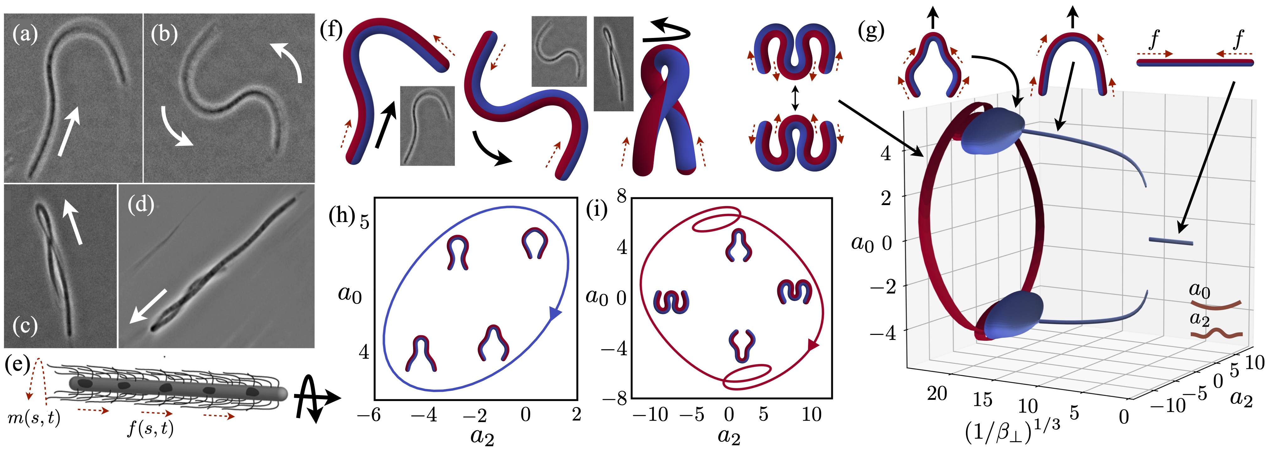
Figure 1: (a-d) Swarmer P. mirabilis cells bend, rotate, and twist under their own flagellar activity (see Supplementary Movies M1-M4). Solid arrows indicate the direction of motion. (e) Flagellar stresses are modeled as a continuous force density $f(s,t)$ and proportional moment density $m=\chi f$ which drives and rotates the body through the fluid. (f) An active swimming Kirchhoff rod reproduces U-shaped swimming, S-shaped rotation, and twisted, rotating swimming states found in experiments. Dashed arrows indicate the direction of local flagellar forcing. (g) Phase projection onto the first two even biharmonic modes for periodic symmetric dynamics with no active moment for a range of $\beta_{\perp}$. Bifurcations from straight filaments to swimming-U shapes, then to periodic waving-U dynamics, then to periodic flapping-W dynamics are observed as the bending stiffness is reduced. (h) A cross-section of the phase diagram in (g) with $\beta_{\perp}=1.3\times 10^{-4}$ (waving-U dynamics). (i) A cross-section of the phase diagram in (g) with $\beta_{\perp}=7.6\times 10^{-5}$ (flapping-W dynamics).

Such active systems are particularly rich, as even passive slender bodies driven by external forces Du Roure et al. (2019) or flows Lindner and Shelley (2015) continue to reveal new buckling behaviors Li et al. (2013); Pham et al. (2015); Manikantan and Saintillan (2015); Liu et al. (2018); Chakrabarti et al. (2020); Floyd et al. (2022). The shapes and dynamics of elongated P. mirabilis cells share many similarities with active or externally forced filaments which exhibit spontaneous symmetry breaking Jayaraman et al. (2012); Ling et al. (2018); Shi et al. (2022). The U- and S-shaped configurations in Fig. 1a-b have been observed numerically in related systems in two dimensions Laskar and Adhikari (2015), as have spiral-shaped configurations Isele-Holder et al. (2015). The response of semi-flexible polymers to molecular-motor-driven stress has seen tremendous interest Winkler et al. (2017), particularly in the context of cytoskeletal networks and interphase chromatin configurations Man and Kanso (2019); Ghosh and Gov (2014); Saintillan et al. (2018).

Flagellar propulsion, however, introduces additional features, for instance a competition between twist/bend elasticity and twist injection Wolgemuth et al. (2000); Lim and Peskin (2004); Powers (2010), and a dynamic rearrangement of flagellar stress. It is plausible that the highly nonlinear twist-bend coupling Goldstein et al. (1998); Goriely and Tabor (1997a) responsible for the emergence of writhing instabilities Goriely and Tabor (1997b) and chiral configurations Nizette and Goriely (1999) in generic elastic filaments is also responsible for the configurations seen in Fig. 1c-d.

In this paper we explore numerically and analytically a Kirchhoff rod model of a long, swimming cell which is driven by active forces and moments associated with flagellar activity. Body dynamics are described using the Euler-Poincaré formalism Gay-Balmaz et al. (2009); Boyer and Renda (2017); Ellis et al. (2011) which leverages the geometric structure of the Euclidean group $SE(3)$ and its Lie algebra $\mathfrak{se}(3)$ to seamlessly incorporate numerous kinematic constraints. The model reproduces both two- and three-dimensional configurations (Fig. 1f) and predicts microorganism buckling and writhing under its own flagellar activity and viscous stress response. Bifurcations in the shapes and dynamics appear as the cell body is made more flexible, including buckling and torsional instabilities commonly observed in passive elastic systems, and new modes of motion are found upon the introduction of the active moment.

The cell is assumed to have length $L$ with uniform circular cross-section of diameter $a$. Aspect ratios $a/L$ of swarmers, typically on the order of $10^{-2}$ to $5\times 10^{-2}$ Hoeniger (1965); Auer et al. (2019c), are sufficiently small that extensile and shear deformations are neglected Antman (1995). Associated with each station of the filament in arclength $s$ and time $t$ is a Euclidean transformation represented as a 4-by-4 matrix $\rho(s,t)=\left(\begin{matrix}Q&\mathbf{r}\\ 0&1\end{matrix}\right)$ which depends on the centerline position $\mathbf{r}$ and orthonormal material frame $Q=[\bm{q}_{0}|\bm{q}_{1}|\bm{q}_{2}]$. Body configurations are written as path ordered exponentials Shapere and Wilczek (1989),

$$\rho(0,t)=\rho(0,0)\text{Pexp}\left(\int_{0}^{t}\psi_{t}(0,\xi)\differential{\xi}\right),$$ (1)

$$\rho(s,t)=\rho(0,t)\text{Pexp}\left(\int_{0}^{s}\psi_{s}(\xi,t)\differential{\xi}\right),$$ (2)

of $\mathfrak{se}(3)$-valued velocities $\psi_{t}=\rho^{-1}\partial_{t}\rho=\left(\begin{matrix}\hat{\bm{\omega}}&\mathbf{u}\\ 0&0\end{matrix}\right)$ and deformations $\psi_{s}=\rho^{-1}\partial_{s}\rho=\left(\begin{matrix}\hat{\bm{\Omega}}&\mathbf{U}\\ 0&0\end{matrix}\right)$, where we have defined the antisymmetric operators $\hat{\bm{\omega}}:=\bm{\omega}\times$ and $\hat{\bm{\Omega}}:=\bm{\Omega}\times$. Working in the local material frame, we formulate dynamics directly in terms linear and angular velocities, $\mathbf{u}=Q^{-1}\partial_{t}\bm{r}$ and $\bm{\hat{\omega}}=Q^{-1}\partial_{t}Q$, respectively, and their space-like analogues, the linear deformation $\mathbf{U}=Q^{-1}\partial_{s}\bm{r}$ and twist/curvature operator $\bm{\hat{\Omega}}=Q^{-1}\partial_{s}Q$. The well known compatibility relations Powers (2010); Antman (1995) for elastic rods are subsumed by the Euclidean structure equations Darling (1994)

$$\partial_{s}\bm{\omega}-\partial_{t}\mathbf{\Omega}+\mathbf{\Omega}\times\bm{\omega}=\mathbf{0},$$ (3)

$$\partial_{s}\mathbf{u}-\partial_{t}\mathbf{U}+\mathbf{\Omega}\times\mathbf{u}-\bm{\omega}\times\mathbf{U}=\mathbf{0},$$ (4)

which ensure the integrability of the system $\rho^{-1}\differential{\rho}=\psi_{s}\differential{s}+\psi_{t}\differential{t}$. A principal advantage of this approach is that it naturally leads to numerical schemes which circumvent violations of inextensibility, unshearbility, and frame orthonormality, and do not require soft penalties or explicit parameterization of rotations by Euler angles or quaternions Iserles et al. (2000); Giusteri and Fried (2018); Park and Chung (2005); Haier et al. (2006); Crouch and Grossman (1993).

Viscous stresses, $\bm{\zeta}\cdot\bm{u}$ and $\zeta_{r}\bm{\omega}_{\parallel}=\left(\bm{U}\cdot\bm{\omega}\right)\bm{U}$, are characterized by the drag tensor, $\bm{\zeta}=\zeta_{\parallel}\mathbf{U}\mathbf{U}^{T}+\zeta_{\perp}(1-\mathbf{U}\mathbf{U}^{T})$ with longitudinal $\zeta_{\parallel}$ and transverse $\zeta_{\perp}$ coefficients, and by a rotational drag coefficient $\zeta_{r}$ Wolgemuth et al. (2000); Wada (2011). Driving the system away from equilibrium are active stresses arising from a distribution of flagella, modeled here as a continuum providing an effective tangential force density $f\mathbf{U}$ and proportional moment density $m\mathbf{U}:=\chi f\mathbf{U}$ (Fig. 1e). To account for the tendency of flagella to align with local flow, we consider $f$ to evolve according to

$$\tau_{f}\partial_{t}f=(F/L)\left[1-(f/F)^{2}\right]\mathbf{U}\cdot\mathbf{u}+D\partial_{s}^{2}f,$$ (5)

with $\partial_{s}f(-L/2)=\partial_{s}f(L/2)=0$. The density tends toward a characteristic magnitude $F$ with a relaxation time $\tau_{f}\zeta_{\parallel}L/F$ depending on the dimensionless parameter $\tau_{f}$, and $D$ is a diffusion constant.

The internal energy of the body is given by $E=\int_{-L/2}^{L/2}\frac{1}{2}\bm{\Omega}\cdot B\bm{\Omega}+\bm{\Lambda}\cdot\bm{U}\differential{s}$, where $\bm{\Lambda}$ is a Lagrange multiplier which enforces inextensibility and unshearability,

$$\mathbf{q}_{0}=Q\mathbf{U}$$ (6)

and $B=B_{\parallel}\mathbf{U}\mathbf{U}^{T}+B_{\perp}(1-\mathbf{U}\mathbf{U}^{T})$ penalizes twisting and bending with moduli $B_{\parallel}$ and $B_{\perp}$, respectively Antman (1995). Balancing structure preserving variations Gay-Balmaz et al. (2009) of $E$ with active and viscous work gives the Euler-Poincaré equations,

$$\bm{\zeta}\cdot\bm{u}=\partial_{s}\bm{\Lambda}+\bm{\Omega}\times\bm{\Lambda}+f\bm{U},$$ (7)

$$\zeta_{r}\bm{\omega}_{\parallel}=\partial_{s}\left(B\mathbf{\Omega}\right)+\mathbf{\Omega}\times B\mathbf{\Omega}+\mathbf{U}\times\mathbf{\Lambda}+m\mathbf{U},$$ (8)

which represent local force and moment balance sup . The kinematic relations (1)-(4),(6), the flagellar evolution law (5), and the balance equations (7),(8) form a closed system describing dynamics of the body and its flagellar distribution.

Using (6)-(8), and the transverse part of (4), we solve for $\bm{U}$, $\bm{u}$, $\bm{\omega}$, and $\bm{\Lambda}_{\perp}:=(1-\mathbf{U}\mathbf{U}^{T})\cdot\bm{\Lambda}$ in terms of the curvature $\bm{\Omega}$, active force density $f$ and tension, $\lambda:=\bm{\Lambda}\cdot\mathbf{U}$. These remaining variables evolve according to (3), (5), and the tangential component of (4), with force and moment-free endpoints requiring $\mathbf{\Omega}$, $\partial_{s}\mathbf{\Omega}_{\perp}$, and $\lambda$ to vanish at the boundaries sup . Equations (1) and (2) are used to locate and orient the body with respect to an inertial frame. Upon scaling by the length $L$, force density $F$, and stiffness $B_{\perp}$, the system is found to depend on five dimensionless groups: a relative bending modulus $\beta_{\perp}=B_{\perp}/(FL^{3})$, twist modulus $\beta_{\parallel}=B_{\parallel}/(FL^{3})$, translational drag ratio $\eta=\zeta_{\perp}/\zeta_{\parallel}$, rotational drag $\eta_{r}=\zeta_{r}/(\zeta_{\parallel}L^{2})$, and scaled active moment $M=\chi/L$.

The equations governing $(\bm{\Omega},f,\lambda)$ are discretized in space uniformly using second-order accurate central difference approximations, and advanced in time using a second-order implicit backward-differentiation scheme with a hybrid nonlinear solver applied at each timestep. Equations (1)-(2) are solved using explicit second-order accurate Magnus integrators Iserles and Nørsett (1999); Blanes et al. (2009); sup . Other approaches to this stiff numerical problem with different treatments of the hydrodynamics have recently been developed Lim (2010); Griffith and Lim (2012); Olson et al. (2013); Lee et al. (2014); Koens and Lauga (2016); Maxian et al. (2022); Walker et al. (2023); Garg and Kumar (2023); Lin et al. (2022); Maxian and Donev (2022). The parameters $(\eta,D,\tau_{f})=(2,10^{-3},10^{-2})$, timestep size $\Delta t=10^{-3}$, and spatial gridspacing $\Delta s=1/64$ are fixed for the duration unless otherwise stated.

In the case of no active moment, $M=0$, the body configuration is fully characterized by a single rotational strain, the (signed) centerline curvature $\kappa=\pm|\Omega_{\perp}|$. Restricting the shape evolution equations to two dimensions, the curvature and tension satisfy

$$\partial_{t}\kappa=-\frac{\beta_{\perp}}{\eta}\partial_{s}^{4}\kappa+\frac{1}{\eta}\partial_{s}^{2}\left(\kappa\lambda\right)\\ +\partial_{s}\left(\kappa\left[\partial_{s}\lambda+f\right]\right)+\frac{\beta_{\perp}}{3}\partial_{s}^{2}\left(\kappa^{3}\right),$$ (9)

and

$$\partial_{s}^{2}\lambda-\frac{\kappa^{2}}{\eta}\lambda=-\partial_{s}f-\frac{\beta_{\perp}}{2}\partial_{s}^{2}\left(\kappa^{2}\right)-\frac{\beta_{\perp}}{\eta}\kappa\partial_{s}^{2}\kappa.$$ (10)

The space of possible body motions is vast, so to begin we consider shapes which are symmetric about the body midpoint $s=0$ (and active forces which are odd). To describe the geometry it is convenient to use the eigenfunctions of $\partial_{s}^{4}$ satisfying force- and moment-free boundary conditions Wiggins et al. (1998) (the first three of which are shown in Fig. 2c as dashed red curves). The curvature is decomposed as a sum $\kappa(s,t)=\sum_{k=0}^{\infty}a_{k}(t)\phi_{k}(s)$. Figure 1g shows a phase portrait for the dynamics of the first two even biharmonic modes, $(a_{0},a_{2})$, for a range of bending stiffness $\beta_{\perp}$ with $M=0$.

Phases in Fig. 1g are identified by examining the long time behaviour of filaments initialized with a compressive active force density $f(s,0)=-\tanh(10s)$. For $\beta_{\perp}>9.1\times 10^{-3}$, the stiff filament relaxes to a straight configuration, with the active stress eventually decaying due to diffusion via Eq. (5). At approximately $\beta_{\perp}=9\times 10^{-3}$ there is a bifurcation to steady state U-shaped swimmers with a nonzero $a_{0}$ which dominates all other modes. Further decreases in stiffness lead to curvature oscillations (this cross-section of the phase diagram is shown in Fig. 1h) and excitation of progressively higher modes. At approximately $\beta_{\perp}=6.8\times 10^{-5}$, another bifurcation is observed to unsteady, periodic flapping dynamics which involve even larger excursions in the phase plane (Fig. 1i), and periodic changes in the swimming direction.

Figure 2: (a) Dominant eigenvalues $\mu_{n}$ of the linearized curvature dynamics with no active moment show the emergence of multiple unstable modes at critical bending stiffnesses; the first at $\beta_{\perp}\approx 1.0\times 10^{-2}$. (b) Growth rates of biharmonic eigenfunctions, $\phi_{n}(s)$, in the fully nonlinear system with $M=0$ (solid lines) and $M=0.01$ (dashed). (c) First three unstable modes of the linearized system (solid), and biharmonic eigenfunctions (dashed).

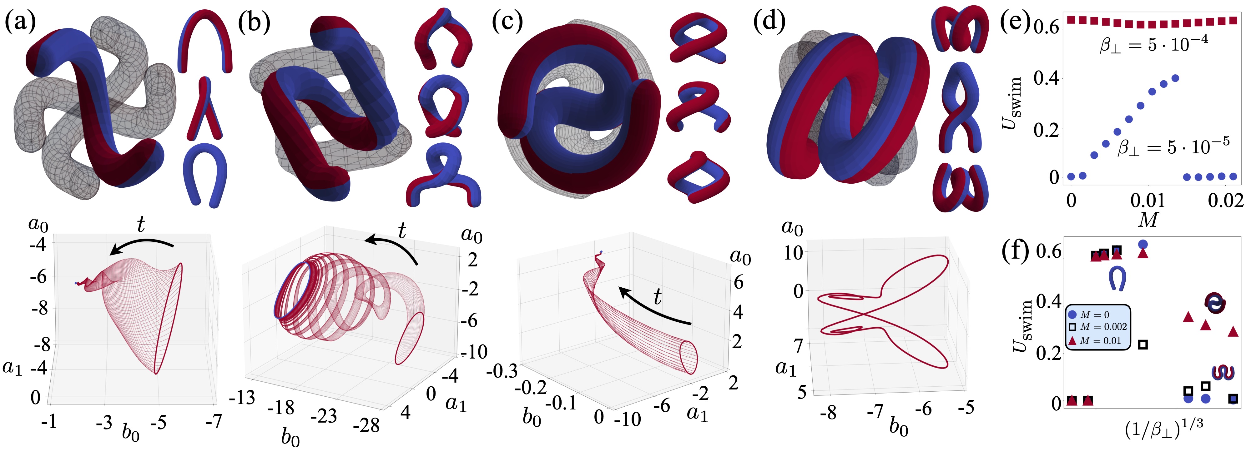
Figure 3: (a-d) New attractors emerge upon the addition of an active moment (with body symmetry assumed). Top - snapshots of body configurations over a half-period, bottom - trajectories of the first two bending ($a_{0},a_{1}$) and the first twisting ($b_{0}$) mode coefficients suggests convergence to a fixed shape. (a) $(\beta_{\parallel},\beta_{\perp},M)=(1\times 10^{-4},2.5\times 10^{-4},6\times 10^{-3})$: a U-shaped swimmer with a twist. (b) $(\beta_{\parallel},\beta_{\perp},M)=(1\times 10^{-5},8\times 10^{-5},1.35\times 10^{-2})$: reduced stiffness and increased active moment introduces a limit cycle corresponding to waving while twisting (see Supplementary Movie M5). (c) $(\beta_{\parallel},\beta_{\perp},M)=(1\times 10^{-3},5.45\times 10^{-5},1\times 10^{-2})$: convergence to a new twisted-S shape. (d) Periodic flapping appears with further increases in $M$ (see Supplementary Movie M6). (e) Swimming speed across a range of active moments for $\beta_{\parallel}=2.5\times 10^{-4}$, for a stiffer ($\beta_{\perp}=5\times 10^{-4}$, squares) and softer ($\beta_{\perp}=5\times 10^{-5}$, circles) body. (f) Swimming speed across a range of bending stiffness for $\beta_{\parallel}=2.5\times 10^{-4}$ and active moments $M=0$ (circles), $M=0.002$ (squares), and $M=0.01$ (triangles).

Susceptibility to buckling can be understood by exploring linear instabilities of a nearly straight body with a symmetric compressive force. Linearization of Eqs. (9)-(10) yields an eigenvalue problem, $\mathcal{L}[\kappa]=\mu\kappa$, where

$$\mathcal{L}[\kappa]=-\frac{\beta_{\perp}}{\eta}\partial_{s}^{4}\kappa-\frac{1}{\eta}\partial_{s}^{2}\left(\kappa\int_{-L/2}^{s}f\differential{s}\right).$$ (11)

Figure 2a shows the (real part) of dominant eigenvalues $\mu_{n}$ of Eq. (11) for a range of stiffness $\beta_{\perp}$. The unstable modes of the linear system are illustrated in Fig. 2c by solid blue curves, along with the biharmonic eigenfunctions for comparison. Growth rates $\sigma_{n}=\left.\partial_{t}a_{n}(t)\right|_{t=0}/a_{n}(0)$, computed using the fully nonlinear system, Eqs. (9)-(10), with $a_{n}(0)=10^{-3}$ are shown in Fig. 2b.

To identify the critical values of $\beta_{\perp}$ where different spatial modes become unstable, we set $\mu=0$ and seek solutions to $\mathcal{L}[\kappa]=0$. For a piecewise constant force density, $f(s)=1-2H(s)$, where $H(s)$ the Heaviside step function, critical values for even modes using Eq. (11) are given by the solutions of

$$\text{Bi}^{\prime}(\xi)\int_{0}^{\xi}\text{Ai}(x)\differential{x}-\text{Ai}^{\prime}(\xi)\int_{0}^{\xi}\text{Bi}(x)\differential{x}=0,$$ (12)

where Ai and Bi are the Airy functions of the first and second kind, and $\xi=-\beta_{\perp}^{-1/3}/2$ sup . For odd modes they are given by solutions of

$$-\xi\text{Bi}(\xi)\int_{0}^{\xi}\text{Ai}(x)\differential{x}+\xi\text{Ai}(\xi)\int_{0}^{\xi}\text{Bi}(x)\differential{x}$$

$$+\text{Bi}^{\prime}(0)\text{Ai}(\xi)-\text{Ai}^{\prime}(0)\text{Bi}(\xi)-1/\pi=0.$$ (13)

When compared to the first ten critical stiffnesses in the fully nonlinear dynamics with regularized active force density, predictions of Eqs. (12)-(13) were found to differ by $0.5\%$-$15\%$. The first bending stiffness below which the filament becomes unstable from the full system is $\beta_{\perp}=1.0\times 10^{-2}$, whereas the linearized dynamics predict $\beta_{\perp}=1.1\times 10^{-2}$.

We turn now to the fully three-dimensional system, including the active moment contribution due to flagellar chirality ($M\neq 0$). Numerous dynamical regimes appear as the result of rotational forcing (see supplementary Movie M7), with transitions between newly emergent phases brought about by variations in any one of the twisting stiffness, $\beta_{\parallel}$, bending stiffness, $\beta_{\perp}$, or active moment, $M$.

As with the 2D system, we seek a reduced order phase space in which to study these bifurcations. To this end, we consider systems initialized with the twist $\Omega_{0}$ and curvature $\Omega_{2}$ even about the midpoint, and the curvature $\Omega_{1}$ odd. This is equivalent to the system possessing a $\pi$-rotational symmetry, and, provided the initial active stress distributions are odd functions of $s$ about the midpoint, this symmetry is conserved. Taking advantage of their conserved parity, the twist and curvatures may be decomposed into sums of harmonic $\gamma_{2k}$ and biharmonic $\{\phi_{2k},\phi_{2k+1}\}$ functions satisfying appropriate parity and boundary and conditions: $\Omega_{0}(s,t)=\sum_{k}b_{2k}(t)\gamma_{2k}(s)$, $\Omega_{1}(s,t)=\sum_{k}a^{(1)}_{2k+1}(t)\phi_{2k+1}(s)$, $\Omega_{2}(s,t)=\sum_{k}a^{(2)}_{2k}(t)\phi_{2k}(s)$.

Figure 3a-d shows characteristic shapes of four observed phases (top), as well as corresponding phase space trajectories of $(b_{0},a_{1},a_{0}):=(b_{0},a_{1}^{(1)},a_{0}^{(2)})$ appearing in the decomposition of twist/curvatures for a range of initial conditions (bottom). For $\beta_{\parallel}<2.5\times 10^{-4}$, $\beta_{\perp}>7.5\times 10^{-4}$, and $M>1.4\times 10^{-2}$ the body adopts a straight configuration. A bifurcation to a twisted-U shape appears upon increasing $\beta_{\parallel}$, decreasing $\beta_{\perp}$, or decreasing $M$ (Fig. 3a). With $M<1.8\times 10^{-2}$, the twisted-$U$ phase persists as $\beta_{\perp}$ is decreased until approximately $\beta_{\perp}=2\times 10^{-4}$, at which point the system develops periodic oscillations (Fig. 3b, see Supplementary Movie M5). Again with $M<1.8\times 10^{-2}$, new S-shaped equilibria emerge for $\beta_{\perp}<1\times 10^{-4}$ (Fig. 3c). A fourth phase appears for $M>1.8\times 10^{2}$ and $\beta_{\perp}<2.5\times 10^{-4}$ with twist-curvature oscillations accompanied by periodic changes in swimming direction (Fig. 3d, see Supplementary Movie M6).

Transitions between phases can lead to wide variations in swimming trajectories, and in the swimming speed, defined as the magnitude of the average velocity of the body’s midpoint in the lab frame, $U_{swim}(T)=\left|\int_{0}^{T}Q(0,t)\mathbf{u}(0,t)\differential{t}\right|/T$. The complicated relationship between bend and twist is further illustrated by the nonmonotonic, and discontinuous, changes in swimming speed that arise due to variations in bending stiffness $\beta_{\perp}$ and active moment $M$. Figure 3e shows the swimming speed as a function of the active moment for two different bending stiffnesses. For the stiffer body the active moment induces waving (from Fig. 3a to Fig. 3b, see Supplementary Movie M5) but the swimming speed remains roughly unchanged. For the softer body, however, which at $M=0$ is in the dramatic flapping-W state in two dimensions (Fig. 1i), the introduction of the active moment can stabilize the shape in three dimensions and result in a ballistic trajectory (Fig. 3c). Further increases in $M$, however, then trigger another phase transition to the three-dimensional flapping dynamics of Fig. 3d (see Supplementary Movie M6), resulting in average speeds (but not instantaneous speeds) tending to zero. A different view is offered by Fig. 3f, which shows the swimming speed across a range of bending stiffnesses for three different active moments. A sufficiently large active moment can delay the onset of flapping dynamics, and thereby stabilize swimming trajectories over a larger range of stiffnesses.

At the lower bending stiffness typical of swarmer cells, rotational forcing introduces a dynamical twist-bend instability. As shown in Fig. 2b as dashed lines for $M=0.01$, the presence of an active moment can decrease the force required to excite higher unstable modes. As described in relation to Fig. 3e above, this allows the system to access new energetically favorable out-of-plane equilibria similar to the ‘locked curvature’ configurations observed in model cilia Ling et al. (2018); Man and Kanso (2019).

Though not explored in detail here, both of the low stiffness configurations shown in Fig. 3c,d are generically unstable with respect to asymmetric perturbations, which lead to non-periodic dynamics and trajectories which depend sensitively upon the bending stiffness (see Supplementary Movie M8). The self-contact evident in Fig. 1d, and self intersections observed at low bending stiffness in the model, suggest that steric interactions are important for stabilizing body configurations of longer swarmer cells. Confinement by neighboring cells in bacterial swarms may play a similar role.

Comparison of our results with experimental observations shows many behaviours of P. mirabilis swarmer cells are captured by the active Kirchhoff rod model. The relative bending stiffness $\beta_{\perp}=B_{\perp}/FL^{3}$, relating the flagellar stress to the cell’s material and geometric properties, is seen to play an outsized role. Our analysis reveals a minimal value, approximately $\beta_{\perp}=1.01\times 10^{-2}$, required of a cell below which its motility is severely hampered by self-buckling. For P. mirabilis swarmer cells, this corresponds to a critical bending stiffness of $B_{\perp}=3\times 10^{-23}\text{Nm}^{2}$, approximately one order of magnitude lower than the experimentally determined stiffness of typical cells Auer et al. (2019c). That the discrepancy is not multiple orders of magnitude suggests that cells may actively maintain mechanical properties to prevent buckling during motility. This is a fascinating observation that may offer insight relevant to the evolutionary development of motility, bacterial adaptation and survival, and potential mechanically-motivated medical interventions. Additional experimental measures of twisting moduli of real biological cells, and more detailed treatment of the hugely complex, flagellated surface, would be needed to further probe this conjecture.

This work was supported by NSF Grant No. DMS-1661900.

References

- Vogel and Stark (2012) R. Vogel and H. Stark, Euro. Phys. J. E 35, 15 (2012).
- Jawed et al. (2015) M. K. Jawed, N. K. Khouri, F. Da, E. Grinspun, and P. M. Reis, Phys. Rev. Lett. 115, 168101 (2015).
- Nguyen and Graham (2018) F. T. M. Nguyen and M. D. Graham, Phys. Rev. E 98, 042419 (2018).
- Zou et al. (2021) Z. Zou, W. Lough, and S. Spagnolie, Phys. Rev. Fluids 6, 103102 (2021).
- Young (2006) K. D. Young, Microbiol. Mol. Biol. Rev. 70, 660 (2006).
- Marshall et al. (2012) W. F. Marshall, K. D. Young, M. Swaffer, E. Wood, P. Nurse, A. Kimura, J. Frankel, J. Wallingford, V. Walbot, X. Qu, et al., BMC Biol. 10, 1 (2012).
- Willis and Huang (2017) L. Willis and K. C. Huang, Nature Rev. Microbiol. 15, 606 (2017).
- Si et al. (2019) F. Si, G. Le Treut, J. T. Sauls, S. Vadia, P. A. Levin, and S. Jun, Curr. Biol. 29, 1760 (2019).
- Avron et al. (2004) J. E. Avron, O. Gat, and O. Kenneth, Phys. Rev. Lett. 93, 186001 (2004).
- Spagnolie and Lauga (2010) S. E. Spagnolie and E. Lauga, Phys. Fluids 22, 031901 (2010).
- Schuech et al. (2019) R. Schuech, T. Hoehfurtner, D. J. Smith, and S. Humphries, Proc. Natl. Acad. Sci. 116, 14440 (2019).
- Tuson et al. (2012) H. H. Tuson, G. K. Auer, L. D. Renner, M. Hasebe, C. Tropini, M. Salick, W. C. Crone, A. Gopinathan, K. C. Huang, and D. B. Weibel, Mol Microbiol. 84, 874 (2012).
- Rojas et al. (2018) E. R. Rojas, G. Billings, P. D. Odermatt, G. K. Auer, L. Zhu, A. Miguel, F. Chang, D. B. Weibel, J. A. Theriot, and K. C. Huang, Nature 559, 617 (2018).
- Al-Mosleh et al. (2022) S. Al-Mosleh, A. Gopinathan, C. D. Santangelo, K. C. Huang, and E. R. Rojas, Proc. Natl. Acad. Sci. 119 (2022).
- Rojas and Huang (2018) E. R. Rojas and K. C. Huang, Curr. Op. Microbiol. 42, 62 (2018).
- Auer et al. (2016) G. K. Auer, T. K. Lee, M. Rajendram, S. Cesar, A. Miguel, K. C. Huang, and D. B. Weibel, Cell systems 2, 402 (2016).
- Auer and Weibel (2017) G. K. Auer and D. B. Weibel, Biochemistry 56, 3710 (2017).
- Rather (2005) P. N. Rather, Env. Microbiol. 7, 1065 (2005).
- Copeland and Weibel (2009) M. F. Copeland and D. B. Weibel, Soft Matter 5, 1174 (2009).
- Auer et al. (2019a) G. K. Auer, P. M. Oliver, M. Rajendram, T.-Y. Lin, Q. Yao, G. J. Jensen, and D. B. Weibel, Mbio 10, e00210 (2019a).
- Auer et al. (2019b) G. K. Auer, P. M. Oliver, M. Rajendram, T.-Y. Lin, Q. Yao, G. J. Jensen, and D. B. Weibel, Mbio 10, e00210 (2019b).
- Trivedi et al. (2018) R. R. Trivedi, J. A. Crooks, G. K. Auer, J. Pendry, I. P. Foik, A. Siryaporn, N. L. Abbott, Z. Gitai, and D. B. Weibel, MBio 9, e01340 (2018).
- Kearns (2010) D. B. Kearns, Nature Rev. Microbiol. 8, 634 (2010).
- Tuson et al. (2013) H. H. Tuson, M. F. Copeland, S. Carey, R. Sacotte, and D. B. Weibel, J. Bacteriol. 195, 368 (2013).
- Blake (1972) J. Blake, J. Fluid Mech. 55, 1 (1972).
- Brennen and Winet (1977) C. Brennen and H. Winet, Ann. Rev. Fluid Mech. 9, 339 (1977).
- Hoeniger (1965) J. F. M. Hoeniger, Microbiol. 40, 29 (1965).
- Lauga (2020) E. Lauga, The fluid dynamics of cell motility, Vol. 62 (Cambridge University Press, 2020).
- Du Roure et al. (2019) O. Du Roure, A. Lindner, E. N. Nazockdast, and M. J. Shelley, Annu. Rev. of Fluid Mech. 51, 539 (2019).
- Lindner and Shelley (2015) A. Lindner and M. Shelley, Fluid-structure interactions in low-Reynolds-number flows 168 (2015).
- Li et al. (2013) L. Li, H. Manikantan, D. Saintillan, and S. E. Spagnolie, J. Fluid Mech. 735, 705 (2013).
- Pham et al. (2015) J. T. Pham, A. Morozov, A. J. Crosby, A. Lindner, and O. du Roure, Phys. Rev. E 92, 011004(R) (2015).
- Manikantan and Saintillan (2015) H. Manikantan and D. Saintillan, Phys. Rev. E 92, 041002(R) (2015).
- Liu et al. (2018) Y. Liu, B. Chakrabarti, D. Saintillan, A. Lindner, and O. Du Roure, Proc. Natl. Acad. Sci. 115, 9438 (2018).
- Chakrabarti et al. (2020) B. Chakrabarti, Y. Liu, J. LaGrone, R. Cortez, L. Fauci, O. du Roure, D. Saintillan, and A. Lindner, Nature Phys. 16, 689 (2020).
- Floyd et al. (2022) C. Floyd, H. Ni, R. S. Gunaratne, R. Erban, and G. A. Papoian, J. Chem. Theory and Comput. 18, 4865 (2022).
- Jayaraman et al. (2012) G. Jayaraman, S. Ramachandran, S. Ghose, A. Laskar, M. S. Bhamla, P. S. Kumar, and R. Adhikari, Phys. Rev. Lett. 109, 158302 (2012).
- Ling et al. (2018) F. Ling, H. Guo, and E. Kanso, J. Roy. Soc. Interface 15, 20180594 (2018).
- Shi et al. (2022) X. Shi, A.-K. Pumm, J. Isensee, W. Zhao, D. Verschueren, A. Martin-Gonzalez, R. Golestanian, H. Dietz, and C. Dekker, Nature Phys. 18, 1105 (2022).
- Laskar and Adhikari (2015) A. Laskar and R. Adhikari, Soft Matter 11, 9073 (2015).
- Isele-Holder et al. (2015) R. E. Isele-Holder, J. Elgeti, and G. Gompper, Soft Matter 11, 7181 (2015).
- Winkler et al. (2017) R. G. Winkler, J. Elgeti, and G. Gompper, Journal of the Physical Society of Japan 86, 101014 (2017).
- Man and Kanso (2019) Y. Man and E. Kanso, Soft Matter 15, 5163 (2019).
- Ghosh and Gov (2014) A. Ghosh and N. Gov, Biophys. J. 107, 1065 (2014).
- Saintillan et al. (2018) D. Saintillan, M. J. Shelley, and A. Zidovska, Proc. Natl. Acad. Sci. 115, 11442 (2018).
- Wolgemuth et al. (2000) C. W. Wolgemuth, T. R. Powers, and R. E. Goldstein, Phys. Rev. Lett. 84, 1623 (2000).
- Lim and Peskin (2004) S. Lim and C. S. Peskin, SIAM J. Sci. Comput. 25, 2066 (2004).
- Powers (2010) T. R. Powers, Rev. Modern Phys. 82, 1607 (2010).
- Goldstein et al. (1998) R. E. Goldstein, T. R. Powers, and C. H. Wiggins, Phys. Rev. Lett. 80, 5232 (1998).
- Goriely and Tabor (1997a) A. Goriely and M. Tabor, Physica D 105, 45 (1997a).
- Goriely and Tabor (1997b) A. Goriely and M. Tabor, Physica D 105, 20 (1997b).
- Nizette and Goriely (1999) M. Nizette and A. Goriely, J. Math. Phys. 40, 2830 (1999).
- Gay-Balmaz et al. (2009) F. Gay-Balmaz, D. D. Holm, and T. S. Ratiu, Journal Of Geometric Mechanics 1, 417 (2009).
- Boyer and Renda (2017) F. Boyer and F. Renda, J. Nonlinear Sci. 27, 1 (2017).
- Ellis et al. (2011) D. C. Ellis, F. Gay-Balmaz, D. D. Holm, and T. S. Ratiu, Journal of Geometry and Physics 61, 2120 (2011).
- Auer et al. (2019c) G. K. Auer, P. M. Oliver, M. Rajendram, T.-Y. Lin, Q. Yao, G. J. Jensen, and D. B. Weibel, Mbio 10 (2019c).
- Antman (1995) S. S. Antman, Nonlinear Problems of Elasticity (Springer, 1995).
- Shapere and Wilczek (1989) A. Shapere and F. Wilczek, J. Fluid Mech. 198, 557 (1989).
- Darling (1994) R. W. R. Darling, Differential Forms and Connections (Cambridge University Press, 1994).
- Iserles et al. (2000) A. Iserles, H. Z. Munthe-Kaas, S. P. Nørsett, and A. Zanna, Acta Numer. 9, 215 (2000).
- Giusteri and Fried (2018) G. G. Giusteri and E. Fried, Journal of Elasticity 132, 43 (2018).
- Park and Chung (2005) J. Park and W.-K. Chung, IEEE Transactions on Robotics 21, 850 (2005).
- Haier et al. (2006) E. Haier, C. Lubich, and G. Wanner, Geometric Numerical Integration: Structure-Preserving Algorithms for Ordinary Differential Equations (Springer, 2006).
- Crouch and Grossman (1993) P. E. Crouch and R. Grossman, Journal of Nonlinear Science 3, 1 (1993).
- Wada (2011) H. Wada, Phys. Rev. E 84, 042901 (2011).
- (66) .
- Iserles and Nørsett (1999) A. Iserles and S. P. Nørsett, Philos. Trans. Royal Soc. A 357, 983 (1999).
- Blanes et al. (2009) S. Blanes, F. Casas, J.-A. Oteo, and J. Ros, Physics reports 470, 151 (2009).
- Lim (2010) S. Lim, Phys. Fluids 22, 024104 (2010).
- Griffith and Lim (2012) B. E. Griffith and S. Lim, Comm. Comput. Phys. 12, 433 (2012).
- Olson et al. (2013) S. D. Olson, S. Lim, and R. Cortez, J. Comput. Phys. 238, 169 (2013).
- Lee et al. (2014) W. Lee, Y. Kim, S. D. Olson, and S. Lim, Phys. Rev. E 90, 033012 (2014).
- Koens and Lauga (2016) L. Koens and E. Lauga, Phys. Fluids 28, 013101 (2016).
- Maxian et al. (2022) O. Maxian, B. Sprinkle, C. S. Peskin, and A. Donev, Phys. Rev. Fluids 7, 074101 (2022).
- Walker et al. (2023) B. J. Walker, K. Ishimoto, and E. A. Gaffney, Phys. Rev. Fluids (2023).
- Garg and Kumar (2023) M. Garg and A. Kumar, Math. Mech. Solids 28, 692 (2023).
- Lin et al. (2022) Y. L. Lin, N. J. Derr, and C. H. Rycroft, Proc. Natl. Acad. Sci. 119, e2105338118 (2022).
- Maxian and Donev (2022) O. Maxian and A. Donev, J. Fluid Mech. 952, A5 (2022).
- Wiggins et al. (1998) C. H. Wiggins, D. Riveline, A. Ott, and R. E. Goldstein, Biophys. J. 74, 1043 (1998).