A Deep solver for BSDEs with jumps

Abstract.

The aim of this work is to propose an extension of the Deep BSDE solver by Han, E, Jentzen (2017) to the case of FBSDEs with jumps. As in the aforementioned solver, starting from a discretized version of the BSDE and parametrizing the (high dimensional) control processes by means of a family of ANNs, the BSDE is viewed as model-based reinforcement learning problem and the ANN parameters are fitted so as to minimize a prescribed loss function. We take into account both finite and infinite jump activity by introducing, in the latter case, an approximation with finitely many jumps of the forward process.

1. Introduction

Forward backward stochastic differential equations (FBSDEs) have become a popular tool in several application domains. One reason is that, due to the Feynman-Kac theorem, they essentially represent the stochastic counterpart of partial differential equations (PDEs): such equations naturally arise when modelling phenomena in diverse fields such as physics, engineering and finance. In finance, for example, PDEs/FBSDEs emerge in the context of the problem of pricing a contingent claim, when the underlying security, i.e. the state variable, is modelled by means of a diffusion process. Similar remarks apply when we consider state variables following a jump diffusion process: in this case a further integral/non local term appears in the Cauchy problem, which is then referred to as a partial integro-differential equation (PIDE). BSDEs in this case are in turn generalized by the introduction of a jump term driven by a Poisson random measure.

When a closed-form solution to the PIDE is not available and the dimension of the vector of state variables is low, several approaches for the numerical solution are availble, the most famous being finite difference and finite element methods. For further details, we refer the reader to Cont and Tankov (2003), Hilber et al. (2013). However, the application of such standard numerical techniques becomes increasingly difficult as the dimension of the state space increases: the tightness of error bounds may be negatively affected or, more simply, the required computational time might increase significantly. Such phenomena are often referred to as the curse of dimension.

The above mentioned problems in a high dimensional setting provide the motivation for the recent surge in interest in machine-learning based methods to solve PDEs/BSDEs, where artificial neural networks (ANNs) are employed in order to parametrize e.g. the function satisfying the PDE and/or its gradient. From a mathematical perspective, ANNs are multiple nested compositions of relatively simple multivariate functions. ANNs can be graphically represented by logical maps with a structure that loosely resembles the one of the human brain, where each neuron (corresponding to the application of a simple function on a multi-dimensional vector) is linked to a multitude of neighboring neurons grouped in sequential layers. The term deep neural networks refers to ANNs with several interconnected layers. One remarkable property of ANNs is given in the ‘Universal Approximation Theorem’, which essentially states that any continuous function in any dimension can be represented to arbitrary accuracy by means of an ANN, and has been proven in different versions, starting from the remarkable insight of Kolmogorov’s Representation Theorem in Kolmogorov (1956) and the seminal works of Cybenko (1989) and Hornik (1991). In a nutshell, this result states that any continuous function in any dimension can be represented to arbitrary accuracy by means of an ANN. Several authors have shown, under different assumption and in different settings, that ANNs can overcome the curse of dimension when approximating the solutions of PDEs, see e.g. Jentzen et al. (2018), Reisinger and Zhang (2020), Hutzenthaler et al. (2018).

Recently, several authors have proposed different numerical schemes for PDEs/BSDEs based on the Feynman-KaKacc theorem in absence of jumps. Seminal works in this sense are E et al. (2017) and Han et al. (2018), together with the convergence study in Han and Long (2020). In these works, the BSDE is discretized forward in time via a standard Euler scheme. The initial condition and the controls of the BSDE, at each point in time, are then parametrized by a family of ANNs. The parameters of the ANNs are optimized by minimizing the expected square distance between the known terminal condition and the terminal value of the discretized BSDE. An alternative route has been followed in Huré et al. (2020). They propose two schemes, DBDP1 and DBDP2, that involve a backward recursion based on the dynamic programming principle. At each time step, they seek to minimize the distance between the BSDE at the subsequent time step and the parametrized dynamics of the BSDE which depends on ANNs. In the first version (DBDP1) two families of neural networks are employed to approximate the value process and the control in the solution of the BSDE. The second version of the algorithm (DBDP2) exploits the fact that the control is linked to the gradient of the value process of the BSDE so that only one family of neutral networks is employed for the approximation of the value process. The control is obtained by automatic differentiation. Another alternative is the so-called deep splitting method, first proposed in Beck et al. (2021): in this case the differential operator of a parabolic PDE is split into a linear and a non-linear part. The non-unique split is chosen is such a way that the non-linear part becomes small. The PDE is then solved iteratively over small time intervals. Such numerical solution involves the recursive computation of conditional expectations which are approximated by means of ANNs. We also mention, among others, the deep Galerkin method proposed in Sirignano and Spiliopoulos (2018): this method is not based on the link between FBSDE and PDEs instead, in their approach, the ANN is trained in order to satisfy the differential operator, the initial condition, and the boundary conditions.

The above mentioned papers have been generalized in a multitude of directions and we refer to Beck et al. (2021) for an extensive literature review.

Concerning the case with jumps the number of studies linking deep learning with the numerical solution of PIDEs is lower. The aforementioned contribution Huré et al. (2020) has been extended to the jump diffusion case in Castro (2021), which also proposes a convergence analysis. A generalization of Beck et al. (2021) is presented in Frey and Köck (2021) with a convergence analysis provided in Frey and Köck (2022). The deep Galerkin method instead is extended in Al-Aradi et al. (2019).

In this paper, we generalize the algorithm of E et al. (2017) and Han et al. (2018) to the jump diffusion setting. Following their reasoning, we discretize the FBSDE with jumps in a forward loop with respect to the time dimension. Next, we introduce deep learning approximations, in the form of two families of ANNs with different tasks: the first family approximates the value process of the BSDE, i.e. the solution of the PIDE, whereas the second is introduced in order to approximate the possibly high dimensional integral with respect to the Lévy measure that appears in the discretized BSDE. Our algorithm is first formulated for processes where the jump term exhibits finite activity. The first family of networks is trained by minimizing the expected square distance between the terminal value of the parametrized BSDE and the known terminal condition, in line with E et al. (2017) and Han et al. (2018). To train the second family of ANNs we exploit the martingale property of compensated Poisson integrals and the $L^{2}$-minimality of conditional expectations, which results in a second penalty term to be minimized. We also propose an extension for the infinite activity/infinite variation of jumps case: we rely on the literature on the approximation of paths of infinite activity Lévy processes by means of compound Poisson processes, (see e.g. Asmussen and Rosiński (2001) among others) and we also introduce a perturbation of the diffusion coefficient to approximate jumps smaller than a pre-specified threshold.

The paper is organized as follows. In Section 2, we present our main assumptions and notations, whereas Section 3 is devoted to the presentation of our algorithm both in the finite and the infinite activity case. Section 4 presents some a priori error estimates that study the distance between the solution of the true FBSDE with jumps of infinite activity and the one of the approximating FBSDE driven by a compound Poisson process. Finally Section 5 presents some numerical experiments both in the finite and infinite activity setting.

2. Setting and preliminaries

We fix a time horizon $T\in\mathbb{R}_{+}$ with $T<\infty$. Let $\left(\Omega,\mathcal{F},\mathbb{F},\mathbb{Q}\right)$ be a filtered probability space, where the filtration $\mathbb{F}=\left(\mathcal{F}_{t}\right)_{t\in[0,T]}$ satisfies the usual assumptions. All semimartingales introduced in the following are càdlàg.

We suppose that the filtered probability space supports an $\mathbb{R}^{d}$ valued standard Brownian motion $W=(W_{t})_{t\in[0,T]}$, together with a Poisson random measure $N$ with associated Lévy measure $\nu$, such that

(2.1) $$\nu(\{0\})=0,\quad\int_{\mathbb{R}^{d}}1\wedge|z|^{2}\nu(\mathrm{d}z)<\infty,\quad\text{ and }\int_{|z|\geq 1}|z|^{2}\nu(\mathrm{d}z)<\infty,$$

allowing us to introduce the compensated random measure

(2.2) $$\tilde{N}(\mathrm{d}t,\mathrm{d}z):=N(\mathrm{d}t,\mathrm{d}z)-\nu(\mathrm{d}z)\mathrm{d}t.$$

Let us introduce the following spaces

• $\mathbb{L}_{\mathcal{F}}^{2}\left(\mathbb{R}^{d}\right)$, the space of all $\mathcal{F}$-measurable random variables $X:\Omega\rightarrow\mathbb{R}^{d}$ satisfying

  $$\|X\|^{2}:=\mathbb{E}\left(|X|^{2}\right)<+\infty;$$

• $\mathbb{H}_{T}^{2}\left(\mathbb{R}^{d}\right)$, the space of all predictable process $\phi:\Omega\times[0,T]\rightarrow\mathbb{R}^{d}$ such that

  $$\|\phi\|^{2}_{\mathbb{H}^{2}}:=\mathbb{E}\left[\int_{0}^{T}\left|\phi_{t}\right|^{2}\mathrm{~{}d}t\right]<+\infty.$$

As previously mentioned, the filtration $\mathbb{F}$ supports the Brownian motion $W$ and the Poisson random measure $N$. The following is the statement of the predictable representation property in the present setting

Lemma 2.1 (See Lemma III, 4.24 in Jacod and Shiryaev (2003)).

Any $\mathbb{F}$ local martingale $M$ has the representation

$$M_{t}=M_{0}+\int_{0}^{t}Z_{s}\mathrm{~{}d}W_{s}+\int_{0}^{t}\int_{\mathbb{R}^{d}}U_{s}(z)\tilde{N}(\mathrm{d}s,\mathrm{d}z),\quad 0\leq t\leq T$$

where $Z$ and $U$ are $\mathbb{F}$-predictable processes both integrable with respect to $W$ and $\tilde{N}$.

Next, we introduce the following spaces that are needed to define the concept of solution to FBSDEs.

• $\mathbb{H}_{T,N}^{2}\left(\mathbb{R}^{d}\right)$ is the space of all predictable process $\phi:\Omega\times[0,T]\times\mathbb{R}^{d}\rightarrow\mathbb{R}^{d}$ satisfying

  $$\|\phi\|^{2}_{\mathbb{H}_{N}^{2}}:=\mathbb{E}\left[\int_{0}^{T}\int_{\mathbb{R}^{d}}\left|\phi_{t}(z)\right|^{2}\nu(\mathrm{d}z)\mathrm{d}t\right]<+\infty,$$

  where we integrate with respect to the predictable compensator of the Poisson random measure $N$.

• $\mathbb{S}_{T}^{2}\left(\mathbb{R}^{d}\right)$ is the space of $\mathbb{F}$-adapted càdlàg processes $\phi:\Omega\times[0,T]\rightarrow\mathbb{R}^{d}$ satisfying

  $$\|\phi\|_{\mathbb{S}^{2}}:=\mathbb{E}\left[\sup_{0\leq t\leq T}\left|\phi_{t}\right|^{2}\right]<+\infty.$$

Let us consider a SDE in the following general form:

(2.3) $$X_{s} =x+\int_{t}^{s}b\left(X_{r-}\right)\mathrm{d}r+\int_{t}^{s}\sigma\left(X_{r-}\right)^{\top}\mathrm{d}W_{r}+\int^{s}_{t}\int_{\mathbb{R}^{d}}\Gamma\left(X_{r-},z\right)\tilde{N}(\mathrm{d}r,\mathrm{d}z),\,\;t\in[0,T],\,x\in\mathbb{R}^{d}.$$

The vector fields $b:\mathbb{R}^{d}\mapsto\mathbb{R}^{d}$, $\sigma:\mathbb{R}^{d}\mapsto\mathbb{R}^{d\times d}$, $\Gamma:\mathbb{R}^{d}\times\mathbb{R}^{d}\mapsto\mathbb{R}^{d}$ are measurable functions satisfying the following assumptions.

• The functions $b$ and $\sigma$ are Lipschitz continuous;

• The function $\Gamma$ satisfies, for some constant $K>0$

  $$\begin{aligned} &\int_{|z|<1}\left|\Gamma\left(x,z\right)-\Gamma\left(x^{\prime},z\right)\right|^{2}\nu(\mathrm{d}z)\leq K\left|x-x^{\prime}\right|^{2}\\ &\int_{|z|<1}|\Gamma(x,z)|^{2}\nu(\mathrm{d}z)\leq K\left(1+|x|^{2}\right)\end{aligned}$$

Under such assumption the SDE (2.3) admits a unique strong solution with initial time $t$ and initial condition $x\in\mathbb{R}^{d}$ that we denote by $X^{t,x}=(X^{t,x}_{s})_{t\in[t,T]}$. In our setting the $\sigma$-algebra $\mathcal{F}_{t}$ is then the trivial one.

Theorem 2.2.

Let assumptions (A1)-(A2) be satisfied. The following holds:

1. for each $(t,x)\in[0,T]\times\mathbb{R}^{d}$ exists a unique adapted, càdlàg solution $X^{t,x}:=$ $(X_{s}^{t,x})_{t\leq s\leq T}$ to (2.3);

2. the solution $X^{t,x}$ is a homogeneous Markov process.

Proof.

The claims follow from Theorem 6.2.9. and Theorem 6.4.6 in Applebaum (2009) respectively. ∎

Let us then introduce the following BSDE:

(2.4) $$Y_{t}= g(X_{T})+\int_{t}^{T}f\left(s,X_{r-},Y_{r-},Z_{r},\int_{\mathbb{R}^{d}}U_{r}(z)\nu(\mathrm{d}z)\right)\mathrm{d}r-\int_{t}^{T}Z_{r}^{\top}\mathrm{d}W_{r}$$

$$-\int^{T}_{t}\int_{\mathbb{R}^{d}}U_{r}(z)\tilde{N}(\mathrm{d}r,\mathrm{d}z).$$

Remark 2.3.

A more general formulation of the BSDE (2.4) may involve a driver of the form $f:[0,T]\times\mathbb{R}^{d}\times\mathbb{R}\times\mathbb{R}^{d}\times L^{2}_{\nu}(\mathbb{R}^{d})\rightarrow\mathbb{R}$, where $L^{2}_{\nu}(\mathbb{R}^{d})$ is the space of functions $\phi$ such that $\int_{\mathbb{R}^{d}}|\phi(z)|^{2}\nu(\mathrm{d}z)<\infty$, i.e. the driver in (2.4) may be replaced by a generic functional $f\left(s,X_{r-},Y_{r-},Z_{r},U_{r}(\cdot)\right)$. We introduce instead a dependence on the integral of $U$ with respect to the Lévy measure, which is often found in applications, see e.g. Delong (2017).

We consider the following assumptions:

1. the function $f:[0,T]\times\mathbb{R}^{d}\times\mathbb{R}\times\mathbb{R}^{d}\times\mathbb{R}^{d}\rightarrow\mathbb{R}$ is Lipschitz continuous with respect to the state variables, uniformly in $t$, i.e. there exists $K>0$ such that

   $$\left|f(t,x,y,z,u)-f\left(t,x^{\prime},y^{\prime},z^{\prime},u^{\prime}\right)\right|$$

   $$\quad\leq K\left(\left|x-x^{\prime}\right|+\left|y-y^{\prime}\right|+\left|z-z^{\prime}\right|+\left|u-u^{\prime}\right|\right)$$

   for all $(t,x,y,z,u),\left(t,x^{\prime},y^{\prime},z^{\prime},u^{\prime}\right)\in[0,T]\times\mathbb{R}^{d}\times\mathbb{R}\times\mathbb{R}^{d}\times\mathbb{R}^{d}$;

2. the function $g:\mathbb{R}^{d}\rightarrow\mathbb{R}$ is Lipschitz continuous, i.e. there exists $K>0$ such that

   $$\left|g(x)-g\left(x^{\prime}\right)\right|\leq K\left|x-x^{\prime}\right|,$$

   for all $x,x^{\prime}\in\mathbb{R}^{d}$.

The above conditions allow us to recall the following existence and uniqueness theorem. We use again superscripts $t,x$ to stress the dependence on the initial condition $x$ at time $t$.

Theorem 2.4.

[Theorem 4.1.3, Delong (2017)] Under assumptions (A1)-(A4) there exists a unique solution $(X^{t,x},Y^{t,x},Z^{t,x},U^{t,x})\in\mathbb{S}_{T}^{2}\left(\mathbb{R}^{d}\right)\times$ $\mathbb{S}_{T}^{2}(\mathbb{R})\times\mathbb{H}_{T}^{2}\left(\mathbb{R}^{d}\right)\times\mathbb{H}_{T,N}^{2}\left({\mathbb{R}}\right)$ to the FBSDE (2.3)-(2.4).

To alleviate notations, hereafter we omit when possible the dependency on the initial condition $(t,x)$ of the processes $(X^{t,x}_{\cdot},Y^{t,x}_{\cdot},Z^{t,x}_{\cdot},U^{t,x}_{\cdot})$.

Our objective is to numerically solve FBSDEs with jumps, possibly in a high dimensional setting, by means of deep learning techniques. It is well known that FBSDEs with jumps are strongly related to PIDEs, so our solver offers in turn a numerical approach to the solution of high dimentional PIDEs. The main theoretical tool that underpins this link is the Feynman-Kac theorem, that links PIDEs and FBSDEs in a Markovian setting. For the reader’s convenience, let us recall the version of the Feynman-Kac theorem that is relevant for our purposes. We are interested in finding a function $u\in C^{1,2}([0,T]\times\mathbb{R}^{d},\mathbb{R})$ that satisfies the PIDE

(2.5) $$\begin{aligned} &-u_{t}(t,x)-\mathscr{L}u(t,x)\\ &\quad-f\left(t,x,u(t,x),D_{x}u(t,x)\sigma(x),\mathscr{J}u(t,x)\right)=0,\quad(t,x)\in[0,T)\times\mathbb{R}^{d},\\ &u(T,x)=g(x),\quad x\in\mathbb{R}^{d},\end{aligned}$$

where

(2.6) $$\begin{aligned} \mathscr{L}u(t,x)=&\left\langle\mu(x),D_{x}u(t,x)\right\rangle+\frac{1}{2}\left\langle\sigma(x)D^{2}_{x}u(t,x),\sigma(x)\right\rangle\\ &+\int_{\mathbb{R}^{d}}\left(u(t,x+\Gamma(x,z))-u(t,x)-\left\langle\Gamma(x,z),D_{x}u(t,x)\right\rangle\right)\nu(dz),\\ \mathscr{J}u(t,x)=&\int_{\mathbb{R}^{d}}(u(t,x+\Gamma(x,z))-u(t,x))\nu(dz).\end{aligned}$$

The link between the FBSDE (2.3)-(2.4) and the PIDE (2.5)-(2.6) is established via the following :

Theorem 2.5 (Theorem 4.2.1, Delong (2017)).

Let assumptions (A1)-(A4) be satisfied and let $u\in C^{1,2}([0,T]\times\mathbb{R}^{d},\mathbb{R})$ satisfy the PIDE (2.5)-(2.6) and the linear growth conditions

(2.7) $$|u(t,x)|\leq K(1+|x|),\quad\left|u_{x}(t,x)\right|\leq K(1+|x|),\quad\forall\,(t,x)\in[0,T]\times\mathbb{R}^{d},$$

then

(2.8) $$\begin{aligned} Y^{t,x}_{s}=&u(s,{X}^{t,x}_{s}),\quad t\leq s\leq T,\\ Z^{t,x}_{s}=&\sigma({X}^{t,x}_{s-})^{\top}D_{x}u(s,{X}^{t,x}_{s-}),\quad t\leq s\leq T,\\ U^{t,x}_{s}(z)=&u(s,{X}^{t,x}_{s-}+\Gamma({X}^{t,x}_{s-},z))-u(s,{X}^{t,x}_{s-}),\quad t\leq s\leq T,z\in\mathbb{R}^{d}.\end{aligned}$$

The above formulation of FBSDEs is intrinsically linked to the following stochastic optimal control problem:

(2.12) $$\underset{\begin{array}[]{c}y\in\mathbb{R},\\ Z\in\mathbb{H}_{T}^{2}\left(\mathbb{R}^{d}\right),\\ U\in\mathbb{H}_{T,N}^{2}\left(\mathbb{R}\right)\end{array}}{\text{minimise}}\mathbb{E}\left[\left(g\left(X^{t,x}_{T}\right)-Y^{y,Z,U}_{T}\right)^{2}\right],$$

(2.13) subject to:

$$\begin{cases}X^{t,x}_{s}=x+\int_{t}^{s}b(X^{t,x}_{r-})\mathrm{d}r+\int_{t}^{s}\sigma(X^{t,x}_{r-})^{\top}\mathrm{d}W_{r}+\int^{s}_{t}\int_{\mathbb{R}^{d}}\Gamma(X^{t,x}_{r-},z)\tilde{N}(\mathrm{d}r,\mathrm{d}z),\\ Y^{y,Z,U}_{s}=y-\int_{t}^{s}f(r,X^{t,x}_{r-},Y^{y,Z,U}_{r-},Z_{r},\int_{\mathbb{R}^{d}}U_{r}(z)\nu(\mathrm{d}z))\mathrm{d}r+\int_{t}^{s}(Z_{r})^{\top}\mathrm{d}W_{r}\\ \quad\quad\qquad+\int^{s}_{t}\int_{\mathbb{R}^{d}}U_{r}(z)\tilde{N}(\mathrm{d}r,\mathrm{d}z),\hfill s\in[t,T].\end{cases}$$

Lemma 2.6.

Under assumptions (A1)-(A4), the minimum in problem (2.12) is achieved and the corresponding minimizer $(y^{\star},Z^{\star},U^{\star})$ is the unique solution to the FBSDE (2.3)-(2.4). In particular, one has

$$\mathbb{E}\left[\left(g\left(X^{t,x}_{T}\right)-Y^{y^{\star},Z^{\star},U^{\star}}_{T}\right)^{2}\right]=0$$

and

$$\begin{aligned} y^{\star}&=Y^{t,x}_{t}=u\left(t,x\right),\\ Z^{\star}_{s}&=Z^{t,x}_{s}=\sigma({X}^{t,x}_{s-})^{\top}D_{x}u(s,{X}^{t,x}_{s-}),\quad t\leq s\leq T,\\ U^{\star}_{s}(z)&=U^{t,x}_{s}(z)=u(s,{X}^{t,x}_{s-}+\Gamma({X}^{t,x}_{s-},z))-u(s,{X}^{t,x}_{s-}),\quad t\leq s\leq T,z\in\mathbb{R}^{d}.\end{aligned}$$

Proof.

Thanks to assumptions (A1)-(A4) the FBSDE (2.3)-(2.4) has a unique solution $({X}^{t,x},{Y}^{t,x},{Z}^{t,x},{U}^{t,x})$ as stated in Theorem 2.4. We consider now $({Y}^{t,x}_{t},{Z}^{t,x},{U}^{t,x})$ as the control of the minimization problem (2.12), observing that the dynamics constraint is satisfied. Since we have ${Y}^{t,x}_{T}=g({X}^{t,x}_{T})$ $\mathbb{P}$-a.s. it means that

$$\mathbb{E}\left[\left(g\left(X^{t,x}_{T}\right)-Y^{{Y}^{t,x}_{t},{Z}^{t,x},{U}^{t,x}}_{T}\right)^{2}\right]=0$$

and the minimum is then achieved at $(y^{\star},Z^{\star},U^{\star})=({Y}^{t,x}_{t},{Z}^{t,x},{U}^{t,x})$. Moreover, any other minimizer should be a solution of the FBSDE, but being such a solution unique we can conclude by Theorem 2.5 that the last statement of the lemma holds. ∎

2.1. The Deep BSDE solver by E-Han-Jentzen

We provide an overview of the algorithm proposed in E et al. (2017). The main idea of their approach is to consider, in a setting without jumps, a discretized version of the stochastic control problem in (2.12) and then approximate, at each time step, the control process by using an artificial neural network (ANN). First of all, let us observe that, in absence of jumps the dynamics constraints in (2.12) becomes

(2.14) $$\begin{cases}X^{t,x}_{s}=x+\int_{t}^{s}b(X^{t,x}_{r-})\mathrm{d}r+\int_{t}^{s}\sigma(X^{t,x}_{r-})^{\top}\mathrm{d}W_{r},\\ Y^{y,Z}_{s}=y-\int_{t}^{s}f(r,X^{t,x}_{r-},Y^{y,Z}_{r-},Z_{r})\mathrm{d}r+\int_{t}^{s}(Z_{r})^{\top}\mathrm{d}W_{r},\hskip 28.45274pt\hfill s\in[t,T],\end{cases}$$

and the control problem (2.12) reduces to an optimization with respect to $y\in\mathbb{R}$ and $Z\in\mathbb{H}_{T}^{2}$. Given $M\in\mathbb{N}$, a time discretization $0\leq t=t_{0}<t_{1}<\ldots<t_{M}=T$ is introduced. For simplicity let us assume that the mesh grid is uniform with step $\Delta t>0$. Let $\Delta W_{n}=W_{t_{n+1}}-W_{t_{n}}$ denote the increments of the Brownian motion. An Euler-Maruyama discretization of the FBSDE is considered, i.e. for $n=0,\ldots,M-1$ we define the following discrete time version of the dynamics (2.14),

(2.15) $$\begin{cases}{\widetilde{X}}_{{n+1}}&={\widetilde{X}}_{n}+b({\widetilde{X}}_{n})\Delta t+\sigma({\widetilde{X}}_{n})\Delta W_{n},\hfill\widetilde{X}_{0}=x,\\ {\widetilde{Y}}_{{n+1}}&={\widetilde{Y}}_{n}-f(t_{n},{\widetilde{X}}_{n},{\widetilde{Y}}_{n},\widetilde{Z}_{n})\Delta t+\widetilde{Z}_{n}^{\top}\Delta W_{n},\hfill\hskip 28.45274pt{\widetilde{Y}}_{0}=y.\end{cases}$$

The next step is to represent, for each $n$, the control process $\widetilde{Z}_{n}$ in (2.15) by using an artificial neural network (ANN). In particular, feedforward ANN with $\mathcal{L}+1\in\mathbb{N}\setminus\{1,2\}$ layers are employed. Each layer consists of $\upsilon_{\ell}$ nodes (also called neurons), for $\ell=0,\ldots,\mathcal{L}$. The $0$-th layer represents the input layer, while the $\mathcal{L}$-th layer is called the output layer. The remaining $\mathcal{L}-1$ layers are hidden layers. For simplicity, we set $\upsilon_{\ell}=\upsilon$, $\ell=1,\ldots,\mathcal{L}-1$. In our setting, the dimension of the input layer is set equal to $d$, i.e. the dimension of the forward process $X$.

A feedforward neural network is a function defined via the composition

$$x\in\mathbb{R}^{d}\longmapsto\mathcal{A}_{\mathcal{L}}\circ\varrho\circ\mathcal{A}_{\mathcal{L}-1}\circ\ldots\circ\varrho\circ\mathcal{A}_{1}(x),$$

where all $\mathcal{A}_{\ell}$, $\ell=1,\ldots,\mathcal{L}$, are affine transformations of the form $\mathcal{A}_{\ell}(x):=\mathcal{W}_{\ell}x+\beta_{\ell}$, $\ell=1,\ldots,\mathcal{L}$, where $\mathcal{W}_{\ell}$ and $\beta_{\ell}$ are matrices and vectors of suitable size called, respectively, weights and biases. The function $\varrho$, called activation function, is a univariate function $\varrho:\mathbb{R}\mapsto\mathbb{R}$ that is applied component-wise to vectors. With an abuse of notation, we denote $\varrho(x_{1},\ldots,x_{\upsilon})=\left(\varrho(x_{1}),\ldots,\varrho(x_{\upsilon})\right).$ The elements of $\mathcal{W}_{\ell}$ and $\beta_{\ell}$ are the parameters of the neural network. One can regroup all parameters in a vector of size $R=\sum_{\ell=0}^{\mathcal{L}}\upsilon_{\ell}(1+\upsilon_{\ell})$.

Let, for each $n=0,\ldots,M-1$, $\mathcal{Z}^{{\rho_{n}}}_{n}:\mathbb{R}^{d}\to\mathbb{R}^{d}$ be an ANN with parameters ${\rho_{n}}\in\mathbb{R}^{R}$. Replacing $Z_{n}$ with $\mathcal{Z}^{{\rho_{n}}}_{n}({\widetilde{X}}_{n})$ in (2.15) one obtains the following dynamics for the process $\widetilde{Y}$ parametrized by $\rho{=(\rho_{0},\ldots,\rho_{M-1})\in(\mathbb{R}^{R})^{M}}$

(2.16) $$\widetilde{Y}^{y,\rho}_{n+1}={\widetilde{Y}^{y,\rho}}_{n}-f(t_{n},{\widetilde{X}}_{n},\widetilde{Y}^{y,\rho}_{n},\mathcal{Z}^{{\rho_{n}}}_{n}({\widetilde{X}}_{{n}}))\Delta t+(\mathcal{Z}^{{\rho_{n}}}_{n}({\widetilde{X}}_{{n}}))^{\top}\Delta W_{n},\hfill\hskip 28.45274pt{\widetilde{Y}^{y,\rho}}_{0}=y.$$

Observe that the solver involves the introduction of $M$ distinct neural networks, one network for each time step.

The family of neural network is then trained simultaneously over a set of simulated Monte Carlo samples of the dynamics via a standard training algorithm such as stochastic gradient descent or its extensions (one notable example in this sense being given by the ADAM algorithm, see Kingma and Ba (2015)) in order to minimize with respect to $y\in\mathbb{R}$ and $\rho\in\mathbb{R}^{R({\mathcal{Z}})}$ the loss function

(2.17) $$\mathbb{E}\left[\left(g(\widetilde{X}_{M})-\widetilde{Y}^{y,\rho}_{M}\right)^{2}\right].$$

3. Deep Solver with jumps

The aim of this section is to present our proposed extension of the Deep BSDE solver of E et al. (2017) to cover the case of the FBSDE with jumps (2.3)-(2.4).

The main challenge in view of the extension is represented by the case where the forward (and consequently the backward) process exhibits infinitely many jumps, be it of finite or infinite variation. Clearly, such jumps cannot be simulated exactly on a pre-specified grid of time instants. This problem has been first encountered in the literature on the discretization and simulation of Lévy-driven stochastic differential equations, see Fournier (2011) among others. For the reader’s convenience, we split the presentation of our solver in two subsections. In the first subsection we only consider the case with finitely many jumps since it can be simulated exactly via an Euler type discretization. In the second subsection we present the additional steps that we propose in order to cover the infinite activity case.

3.1. Finite activity case

In this subsection we assume that the Lévy measure satisfies the condition $\nu(\mathbb{R}^{d})<\infty$, meaning that the jumps are those of a compound Poisson process. We fix $M\in\mathbb{N}$ and introduce a uniform time discretization $0\leq t=t_{0}<t_{1}<\ldots<t_{M}=T$ with time step $\Delta t>0$. As a starting point, we consider the forward SDE (2.3) between two subsequent time steps $t_{n}$ and $t_{n+1}$, namely,

$$X_{t_{n+1}} =X_{t_{n}}+\int_{t_{n}}^{t_{n+1}}b\left(X_{r-}\right)\mathrm{d}r+\int_{t_{n}}^{t_{n+1}}\sigma\left(X_{r-}\right)^{\top}\mathrm{d}W_{r}+\int^{t_{n+1}}_{t_{n}}\int_{\mathbb{R}^{d}}\Gamma\left(X_{r-},z\right)\tilde{N}(\mathrm{d}r,\mathrm{d}z),$$

with $X_{t_{0}}=x\in\mathbb{R}^{d}$. We freeze the coefficients between to consecutive time steps introducing the discrete time process $\widetilde{X}=(\widetilde{X}_{n})_{n=0,\ldots,M}$, defined recursively by

$$\widetilde{X}_{n+1}=\widetilde{X}_{{n}}+\int_{t_{n}}^{t_{n+1}}b(\widetilde{X}_{n})\mathrm{d}r+\int_{t_{n}}^{t_{n+1}}\sigma(\widetilde{X}_{n})^{\top}\mathrm{d}W_{r}+\int^{t_{n+1}}_{t_{n}}\int_{\mathbb{R}^{d}}\Gamma(\widetilde{X}_{n},z)\tilde{N}(\mathrm{d}r,\mathrm{d}z),\qquad n=0,\ldots,M-1,$$

with $\widetilde{X}_{0}=x.$ We write $N([0,t_{n}],\mathbb{R}^{d})$ to denote the number of $\mathbb{R}^{d}$-valued jump sizes occurring over the time interval $[0,t_{n}]$. The previous equation can then be rewritten as

(3.1) $$\begin{aligned} \widetilde{X}_{n+1}&=\widetilde{X}_{n}+b(\widetilde{X}_{n})\Delta t+\sigma(\widetilde{X}_{n})^{\top}\Delta W_{n}\\ &\quad+\sum_{i=N([0,t_{n}],\mathbb{R}^{d})+1}^{N([0,t_{n+1}],\mathbb{R}^{d})}\Gamma(\widetilde{X}_{n},z_{i})-\Delta t\int_{\mathbb{R}^{d}}\Gamma(\widetilde{X}_{n},z)\nu(\mathrm{d}z),\qquad n=0,\ldots,M-1.\end{aligned}$$

We proceed similarly for the backward dynamics (2.4). We consider again two consecutive time instants $t_{n}$ and $t_{n+1}$

$$Y_{t_{n+1}}= Y_{t_{n}}-\int_{t_{n}}^{t_{n+1}}f\Big{(}r,X_{r-},Y_{r-},Z_{r},\int_{\mathbb{R}^{d}}U_{r}(z)\nu(\mathrm{d}z)\Big{)}\mathrm{d}r+\int_{t_{n}}^{t_{n+1}}Z_{r}^{\top}\mathrm{d}W_{r}+\int_{t_{n}}^{t_{n+1}}\int_{\mathbb{R}^{d}}U_{r}(z)\tilde{N}(\mathrm{d}r,\mathrm{d}z).$$

We now make use of the Feynman-Kac Theorem 2.5, meaning that above dynamics can be read as follows

$$Y_{t_{n+1}} =Y_{t_{n}}-\int_{t_{n}}^{t_{n+1}}f\Big{(}r,X_{r-},Y_{r-},\sigma({X}_{r-})^{\top}D_{x}u(r,{X}_{r-}),\int_{\mathbb{R}^{d}}u(r,X_{r-}+\Gamma(X_{r_{-}},z))-u(r,X_{r-})\nu(\mathrm{d}z)\Big{)}\mathrm{d}r$$

$$\quad+\int_{t_{n}}^{t_{n+1}}(D_{x}u(r,{X}_{r-}))^{\top}\sigma({X}_{r-})\mathrm{d}W_{r}$$

$$\quad+\int_{t_{n}}^{t_{n+1}}\int_{\mathbb{R}^{d}}u(r,X_{r-}+\Gamma(X_{r_{-}},z))-u(r,X_{r-})\tilde{N}(\mathrm{d}r,\mathrm{d}z).$$

Next, we freeze again the coefficients and consider the following discrete time approximation

$$\widetilde{Y}_{{n+1}}= \widetilde{Y}_{{n}}-f\Big{(}t_{n},\widetilde{X}_{{n}},\widetilde{Y}_{{n}},\sigma(\widetilde{X}_{n})^{\top}D_{x}u(t_{n},\widetilde{X}_{n}),\int_{\mathbb{R}^{d}}u(t_{n},\widetilde{X}_{n}+\Gamma(\widetilde{X}_{n},z))-u(t_{n},\widetilde{X}_{n})\nu(\mathrm{d}z)\Big{)}\Delta t$$

$$+(D_{x}u(t_{n},\widetilde{X}_{n}))^{\top}\sigma(\widetilde{X}_{n})\Delta W_{n}$$

$$+\sum_{i=N([0,t_{n}],\mathbb{R}^{d})+1}^{N([0,t_{n+1}],\mathbb{R}^{d})}u(t_{n},\widetilde{X}_{n}+\Gamma(\widetilde{X}_{n},z_{i}))-u(t_{n},\widetilde{X}_{n})$$

$$-\Delta t\int_{\mathbb{R}^{d}}u(t_{n},\widetilde{X}_{n}+\Gamma(\widetilde{X}_{n},z))-u(t_{n},\widetilde{X}_{n})\nu(\mathrm{d}z).$$

At this point, we introduce neural network approximations. We shall introduce 2 distinct $M$-dimensional families of neural network in the solution of the FBSDE (2.3)-(2.4).

We employ the first family of networks to parametrize the function $u$, thus introducing the neural network approximation $\mathcal{U}_{n}^{{\rho_{n}}}:\mathbb{R}^{d}\mapsto\mathbb{R}^{d}$, $n=0,\ldots,M-1$, parametrized by $\rho{=(\rho_{0},\ldots,\rho_{M-1})\in(\mathbb{R}^{R})^{M}}$ and indexed by the time discretization $n\in\{0,\ldots,M-1\}$. Notice that, due to the Feynman-Kac theorem, the control $Z$ depends on the gradient of the function $u$, meaning that, in the numerical scheme, we need to compute the gradient of the neural network. The computation of the gradient of $\mathcal{U}_{n}^{{\rho_{n}}}$ at each time step involves an application of the chain rule for differentiation. This can be easily implemented by relying on Tensorflow’s automatic differentiation capabilities. In our numerical experiments we make use of a sigmoid activation function $\varrho(x)=\frac{1}{1+e^{-x}}$ in order to guarantee differentiability.

Introducing the family of networks ${(\mathcal{U}_{n}^{\rho_{n}})_{n=0,\ldots,M-1}}$ makes it possible to obtain a straightforward approximation for both the stochastic integral with respect to the Brownian motion and the one with respect to the uncompensated Poisson random measure, leaving the question of approximating the compensator term, namely

(3.2) $$\int_{\mathbb{R}^{d}}u(t_{n},\widetilde{X}_{n}+\Gamma(\widetilde{X}_{n},z))-u(t_{n},\widetilde{X}_{n})\nu(\mathrm{d}z),$$

open. Once replaced $u{(t_{n},\cdot)}$ by the ANN $\mathcal{U}^{{\rho_{n}}}_{n}$, thus obtaining

$$\int_{\mathbb{R}^{d}}\mathcal{U}^{\rho_{n}}_{n}(\widetilde{X}_{n}+\Gamma(\widetilde{X}_{n},z))-\mathcal{U}^{\rho_{n}}_{n}(\widetilde{X}_{n})\nu(\mathrm{d}z),$$

the first option, which is feasible when the dimension $d$ is low, is to employ a standard quadrature rule. When the dimension increases one can resort to Monte Carlo integration. However, the training of the networks we introduced involves a further Monte Carlo simulation during the training phase, so that such approach would lead to costly nested Monte Carlo simulations.

We propose a different approach, where at each time step $t_{n}$, we approximate (3.2) via a second family of neural networks $\mathcal{V}_{n}^{{\theta_{n}}}:\mathbb{R}^{d}\to\mathbb{R}$, $n=0\ldots,M-1$, parametrized by $\theta{=(\theta_{0},\ldots,\theta_{M-1})\in(\mathbb{R}^{R})^{M}}$. Here, with the sole aim of simplifying the notation, we are assuming that the size of the parameter vector of every ANN involved in the solver is equal to $R$. Let us recall that the stochastic integral with respect to the compensated Poisson random measure is a square integrable martingale under our assumptions, meaning that

$$\mathbb{E} \left[\left.\int_{t_{n}}^{t_{n+1}}\int_{\mathbb{R}^{d}}u\left(r,X_{r-}+\Gamma(X_{r_{-}},z)\right)-u\left(r,X_{r-}\right)\tilde{N}(\mathrm{d}r,\mathrm{d}z)\right|\mathcal{F}_{t_{n}}\right]=0.$$

Let us recall that the conditional expectation of a random variable $\mathscr{X}\in\mathbb{L}^{2}_{\mathcal{F}}(\mathbb{R})$ with respect to $\mathcal{F}_{t_{n}}\subset\mathcal{F}$ satisfies

$$\mathbb{E}\left[\left.\mathscr{X}\right|\mathcal{F}_{t_{n}}\right]=\operatorname*{arg\,min}_{\widetilde{\mathscr{X}}\in\mathbb{L}^{2}_{\mathcal{F}_{t_{n}}}(\mathbb{R})}\mathbb{E}\left[(\mathscr{X}-\widetilde{\mathscr{X}})^{2}\right]$$

so that, setting $\mathscr{X}=\int_{t_{n}}^{t_{n+1}}\int_{\mathbb{R}^{d}}u\left(r,X_{r-}+\Gamma(X_{r_{-}},z)\right)-u\left(r,X_{r-}\right)\tilde{N}(\mathrm{d}r,\mathrm{d}z)$ we are led to

$$0=\operatorname*{arg\,min}_{\widetilde{\mathscr{X}}\in\mathbb{L}^{2}_{\mathcal{F}_{t_{n}}}(\mathbb{R})}\mathbb{E}\left[(\int_{t_{n}}^{t_{n+1}}\int_{\mathbb{R}^{d}}u\left(r,X_{r-}+\Gamma(X_{r_{-}},z)\right)-u\left(r,X_{r-}\right)\tilde{N}(\mathrm{d}r,\mathrm{d}z)-\widetilde{\mathscr{X}})^{2}\right],$$

which inspires the introduction of a further penalty term to be minimized during the training phase in addition to (2.17): at each time $t_{n}$, we would like to minimize the quantity

$$\mathbb{E}\left[\left(\sum_{i=N([0,t_{n}],\mathbb{R}^{d})+1}^{N([0,t_{n+1}],\mathbb{R}^{d})}\left(\mathcal{U}_{n}^{{\rho_{n}}}(\widetilde{X}_{n}+\Gamma(\widetilde{X}_{n},z_{i}))-\mathcal{U}_{n}^{{\rho_{n}}}(\widetilde{X}_{n})\right)-\Delta t\mathcal{V}_{n}^{{\theta_{n}}}(\widetilde{X}_{n})\right)^{2}\right].$$

This concludes the description of the algorithm for the finite activity case. To summarize, our approach considers the following discretized stochastic control problem

(3.3) $$\begin{aligned} &\underset{\begin{subarray}{c}y\in\mathbb{R},\\ \rho\in{(\mathbb{R}^{R(\mathcal{U})})^{M}},\\ \theta\in{(\mathbb{R}^{R(\mathcal{V})})^{M}}\end{subarray}}{\text{minimise}}\quad\mathbb{E}\left[\left(g(\widetilde{X}_{M})-\widetilde{Y}_{M}^{y,\rho,\theta}\right)^{2}\right]\\ &\qquad\quad+\sum_{n=0}^{M-1}\mathbb{E}\left[\left(\sum_{i=N([0,t_{n}],\mathbb{R}^{d})+1}^{N([0,t_{n+1}],\mathbb{R}^{d})}\left(\mathcal{U}_{n}^{{\rho_{n}}}(\widetilde{X}_{n}+\Gamma(\widetilde{X}_{n},z_{i}))-\mathcal{U}_{n}^{{\rho_{n}}}(\widetilde{X}_{n})\right)-\Delta t\mathcal{V}_{n}^{{\theta_{n}}}(\widetilde{X}_{n})\right)^{2}\right]\end{aligned}$$

subject to:

$$\begin{cases}\widetilde{X}_{n+1}=&\widetilde{X}_{n}+b(\widetilde{X}_{n})\Delta t+\sigma(\widetilde{X}_{n})^{\top}\Delta W_{n}\\ &+\sum_{i=N([0,t_{n}],\mathbb{R}^{d})+1}^{N([0,t_{n+1}],\mathbb{R}^{d})}\Gamma(\widetilde{X}_{n},z_{i})-\Delta t\int_{\mathbb{R}^{d}}\Gamma(\widetilde{X}_{n},z)\nu(\mathrm{d}z)\vspace{0.1cm}\\ \widetilde{Y}^{y,\rho,\theta}_{n+1}=&\widetilde{Y}^{y,\rho,\theta}_{n}-f\left(t_{n},\widetilde{X}_{n},\widetilde{Y}^{y,\rho,\theta}_{n},\sigma(\widetilde{X}_{n})^{\top}D_{x}{\mathcal{U}^{\rho_{n}}_{n}(\widetilde{X}_{n})},\mathcal{V}_{n}^{{\theta_{n}}}(\widetilde{X}_{n})\right)\Delta t\\ &+(D_{x}{\mathcal{U}^{\rho_{n}}_{n}(\widetilde{X}_{n})})^{\top}\sigma(\widetilde{X}_{n})\Delta W_{n}\\ &+\sum_{i=N([0,t_{n}],\mathbb{R}^{d})+1}^{N([0,t_{n+1}],\mathbb{R}^{d})}\left(\mathcal{U}_{n}^{{\rho_{n}}}(\widetilde{X}_{n}+\Gamma(\widetilde{X}_{n},z_{i}))-\mathcal{U}_{n}^{{\rho_{n}}}(\widetilde{X}_{n})\right)-\Delta t\mathcal{V}_{n}^{{\theta_{n}}}\left(\widetilde{X}_{n}\right).\end{cases}$$

3.2. Infinite activity case

To cover the case where the forward process $X$ exhibits infinitely many jumps, we will proceed by introducing an approximating jump diffusion $X^{\epsilon}$ with finitely many jumps, meaning that the jump component will correspond to a compound Poisson process. The small jumps might be truncated or, as we do, they could be approximated via the diffusion term by increasing the volatility. This will constitute the first source of numerical error of our algorithm. Concerning this first approximation step for the forward SDE for $X$ we follow, among others Asmussen and Rosiński (2001), Cohen and Rosiński (2007) and Jum (2015)

Moving from the process $X$ to the process $X^{\epsilon}$ has an implication on the FBSDE as well. To proceed, we will need to introduce some additional assumptions, in particular regarding the structure of the Poisson random measure: let $\epsilon\in(0,1]$. We define

$$\nu^{\epsilon}(\mathrm{d}z):=\mathbbm{1}_{\{|z|>\epsilon\}}\nu(\mathrm{d}z),$$

$$\nu_{\epsilon}(\mathrm{d}z):=\mathbbm{1}_{\{|z|\leq\epsilon\}}\nu(\mathrm{d}z),$$

so that we write

$$\nu=\nu_{\epsilon}+\nu^{\epsilon}.$$

From the definition of the Lévy measure $\nu$ we immediately have $\int_{\mathbb{R}^{d}}|z|^{2}\nu_{\epsilon}(dz)<\infty\;$. We need the following additional assumption

• We assume $\;\nu^{\epsilon}\left(\mathbb{R}^{d}\right)<\infty\;$.

The assumption above means that we can can factorize the jump term in two components, the first one corresponding to the small jumps, and the second one to the big jumps, i.e. a compound Poisson process. The factorization of the Lévy measure means that we are assuming that we can write the Poisson Random Measure $N$ as

(3.4) $$N=N_{\epsilon}+N^{\epsilon}\;,$$

with $N_{\epsilon}$ and $N^{\epsilon}$ having the compensator $\nu_{\epsilon}$ and $\nu^{\epsilon}$, respectively.

In line with Cohen and Rosiński (2007) we introduce the following quantity

$$\Sigma_{\epsilon}:=\int_{\mathbb{R}^{d}}zz^{\top}\nu_{\epsilon}(\mathrm{d}z)=\int_{|z|<\epsilon}zz^{\top}\nu(\mathrm{d}z),$$

taking values in the cone of positive semidefinite $d\times d$ matrices $S^{d}_{+}$. We also introduce a further assumption on the jump term of the forward SDE:

• the function $\Gamma:\mathbb{R}^{d}\times\mathbb{R}^{d}\to\mathbb{R}^{d}$ is of the form

  $$\Gamma(x,z):=\gamma(x)z$$

  for some Lipschitz continuous function $\gamma:\mathbb{R}^{d}\mapsto\mathbb{R}^{d\times d}$.

The remaining assumptions on the vector fields $b,\sigma,\Gamma$ are unchanged with respect to (2.3).

Given $(t,x)\in[0,T]\times\mathbb{R}^{d}$, we approximate the solution $X^{t,x}_{\cdot}$ of the forward SDE (2.3) by means of the process $X^{\epsilon,t,x}_{\cdot}$, whose dynamics are

(3.5) $$\begin{aligned} X^{\epsilon,t,x}_{s}=&x+\int_{t}^{s}b(X^{\epsilon,t,x}_{r-})\mathrm{d}r+\int_{t}^{s}\sigma(X^{\epsilon,t,x}_{r-})^{\top}+\gamma(X^{\epsilon,t,x}_{r-})\sqrt{\Sigma_{\epsilon}}\mathrm{d}W_{r}+\int^{s}_{t}\int_{\mathbb{R}^{d}}\gamma(X^{\epsilon,t,x}_{r-})z\tilde{N}^{\epsilon}(\mathrm{d}r,\mathrm{d}z),\end{aligned}$$

where $\sqrt{\Sigma_{\epsilon}}$ denotes the matrix square root of $\Sigma_{\epsilon}\in S^{d}_{+}$ and we set $\tilde{N}^{\epsilon}:=N^{\epsilon}(\mathrm{d}r,\mathrm{d}z)-\nu^{\epsilon}(\mathrm{d}z)\mathrm{d}r$. Again, whenever possible, we will simply use the notation $X^{\epsilon}$, thus neglecting the dependence on the starting point $(t,x)$. A priori error estimates of the error we introduce by approximating $X$ via $X^{\epsilon}$ can be derived following, for instance, Cohen and Rosiński (2007) and Jum (2015) and will be discussed in the next section.

At this point we apply the solver as described in Section 3.1 to the following BSDE

$$Y^{\epsilon\epsilon}_{t}= g(X^{\epsilon}_{T})+\int_{t}^{T}f(s,X^{\epsilon}_{r-},Y^{\epsilon\epsilon}_{r-},Z^{\epsilon\epsilon}_{r},\int_{\mathbb{R}^{d}}U^{\epsilon\epsilon}(r,z)\nu^{\epsilon}(\mathrm{d}z))\mathrm{d}r-\int_{t}^{T}{Z^{\epsilon\epsilon}_{r}}^{\top}\mathrm{d}W_{r}$$

(3.6) $$-\int^{T}_{t}\int_{\mathbb{R}^{d}}U^{\epsilon\epsilon}_{r}(z)\tilde{N}^{\epsilon}(\mathrm{d}r,\mathrm{d}z).$$

whose solution $(Y^{\epsilon\epsilon},Z^{\epsilon\epsilon},U^{\epsilon\epsilon})$ is intended to approximate $(Y,Z,U)$ solving (2.4).

4. Error estimates

In this section we present a priori error estimates for the error introduced by the approximation of small jumps in the infinite activity case on the solution of the FBSDE.

4.1. A priori error estimates for the forward approximation

We start by providing the $L^{2}$ estimate of the error that we introduce by approximating $X_{\cdot}$ via $X^{\epsilon}_{\cdot}$. We report the full derivation, obtained following Cohen and Rosiński (2007) and Jum (2015), for the sake of completeness. We first have the following moment bound:

Lemma 4.1.

Under the assumptions (A1)-(A2), (A5)-(A6), the SDE (3.5) admits a unique solution $X^{\epsilon}:=(X_{s}^{\epsilon})_{t\leq s\leq T}$. Moreover, there exists $C>0$ such that the following estimate holds

(4.1) $$\mathbb{E}\left[\sup_{s\in[t,T]}\left|X^{\epsilon}_{s}\right|^{2}\right]\leq C\left(1+|x|^{2}\right),\qquad\forall(t,x)\in[0,T]\times\mathbb{R}^{d}.$$

Proof.

Existence and uniqueness follow from the same arguments used for (2.3). We concentrate on the estimate in the following.

$$\mathbb{E}\left[\sup_{s\in[t,T]}\left|X^{\epsilon}_{s}\right|^{2}\right]$$

$$\ \leq C\left(|x|^{2}+\mathbb{E}\left[\int_{t}^{T}\left|b\left(X^{\epsilon}_{r-}\right)\right|^{2}\mathrm{d}r\right]\right.$$

$$\ \ \left.+\mathbb{E}\left[\sup_{s\in[t,T]}\left|\int_{t}^{s}\sigma\left(X^{\epsilon}_{r-}\right)^{\top}+\gamma\left(X^{\epsilon}_{r-}\right)\sqrt{\Sigma_{\epsilon}}\mathrm{d}W_{r}\right|^{2}\right]+\mathbb{E}\left[\sup_{s\in[t,T]}\left|\int^{s}_{t}\int_{\mathbb{R}^{d}}\gamma\left(X^{\epsilon}_{r-}\right)z\tilde{N}^{\epsilon}(\mathrm{d}r,\mathrm{d}z)\right|^{2}\right]\right)\;.$$

Using the Burkholder-Davis-Gundy inequality or equivalently Theorem 2.11 in Kunita (2004) we have

$$\mathbb{E}\left[\sup_{s\in[t,T]}\left|X^{\epsilon}_{s}\right|^{2}\right]$$

$$\ \leq C\left(|x|^{2}+\mathbb{E}\left[\int_{t}^{T}\left|b\left(X^{\epsilon}_{r-}\right)\right|^{2}\mathrm{d}r\right]\right.$$

$$\ \ \left.+\mathbb{E}\left[\int_{t}^{T}\left|\sigma\left(X^{\epsilon}_{r-}\right)^{\top}+\gamma\left(X^{\epsilon}_{r-}\right)\sqrt{\Sigma_{\epsilon}}\right|^{2}\mathrm{d}r\right]+\mathbb{E}\left[\int_{t}^{T}\int_{\mathbb{R}^{d}}\left|\gamma\left(X^{\epsilon}_{r-}\right)z\right|^{2}\nu^{\epsilon}(\mathrm{d}z)\mathrm{d}r\right]\right)$$

We use the fact that $\sup_{\epsilon\in(0,1]}|\sqrt{\Sigma_{\epsilon}}|<\infty$, together with $\int_{\mathbb{R}^{d}}|z|^{2}\nu^{\epsilon}(\mathrm{d}z)<\infty$ (which is a direct consequence of Assumption (A5)) and the Lipschitz continuity of $b,\sigma$ and $\gamma$ so that, redefining the constant $C$ we have

$$\mathbb{E}\left[\sup_{s\in[t,T]}\left|X^{\epsilon}_{s}\right|^{2}\right]\leq C\left(1+|x|^{2}+\mathbb{E}\left[\int_{t}^{T}|X^{\epsilon}_{r}|^{2}\mathrm{d}r\right]\right)\;.$$

Using Gronwall’s inequality we obtain the claim. ∎

Proposition 4.2.

Under the assumptions (A1)-(A2), (A5)-(A6), there exists a constant $C>0$ such that

(4.2) $$\mathbb{E}\left[\sup_{s\in[t,T]}\left|X_{s}-X^{\epsilon}_{s}\right|^{2}\right]\leq C(1+|x|^{2})\int_{\mathbb{R}^{d}}|z|^{2}\nu_{\epsilon}(\mathrm{d}z),\qquad\forall(t,x)\in[0,T]\times\mathbb{R}^{d}.$$

Proof.

$$\mathbb{E} \left[\sup_{s\in[t,T]}\left|X_{s}-X^{\epsilon}_{s}\right|^{2}\right]$$

$$\quad=\mathbb{E}\left[\sup_{s\in[t,T]}\left|\int_{t}^{s}b\left(X_{r-}\right)-b\left(X^{\epsilon}_{r-}\right)\mathrm{d}r+\int_{t}^{s}\sigma\left(X_{r-}\right)^{\top}-\sigma\left(X^{\epsilon}_{r-}\right)^{\top}-\gamma\left(X^{\epsilon}_{r-}\right)\sqrt{\Sigma_{\epsilon}}\mathrm{d}W_{r}\right.\right.$$

$$\quad\quad\quad\quad\quad\quad\left.\left.+\int^{s}_{t}\int_{\mathbb{R}^{d}}\gamma\left(X_{r-}\right)z\tilde{N}(\mathrm{d}r,\mathrm{d}z)-\int^{s}_{t}\int_{\mathbb{R}^{d}}\gamma\left(X^{\epsilon}_{r-}\right)z\tilde{N}^{\epsilon}(\mathrm{d}r,\mathrm{d}z)\right|^{2}\right]$$

$$\quad=\mathbb{E}\left[\sup_{s\in[t,T]}\bigg{|}\int_{t}^{s}b\left(X_{r-}\right)-b\left(X^{\epsilon}_{r-}\right)\mathrm{d}r+\int_{t}^{s}\sigma\left(X_{r-}\right)^{\top}-\sigma\left(X^{\epsilon}_{r-}\right)^{\top}-\gamma\left(X^{\epsilon}_{r-}\right)\sqrt{\Sigma_{\epsilon}}\mathrm{d}W_{r}\right.$$

$$\quad\quad\quad\quad\quad\quad+\int^{s}_{t}\int_{\mathbb{R}^{d}}\gamma\left(X_{r-}\right)z\tilde{N}(\mathrm{d}r,\mathrm{d}z)-\int^{s}_{t}\int_{\mathbb{R}^{d}}\gamma\left(X^{\epsilon}_{r-}\right)z(\underbrace{N-\nu^{\epsilon}-\nu_{\epsilon}}_{\tilde{N}})(\mathrm{d}r,\mathrm{d}z)$$

$$\quad\quad\quad\quad\quad\quad\left.+\int^{s}_{t}\int_{\mathbb{R}^{d}}\gamma\left(X^{\epsilon}_{r-}\right)z(\underbrace{N_{\epsilon}-\nu_{\epsilon}}_{\tilde{N}_{\epsilon}})(\mathrm{d}r,\mathrm{d}z)\bigg{|}^{2}\right].$$

As in Jum (2015), we now use Theorem 2.11 in Kunita (2004) with $p=2$ and obtain

$$\mathbb{E} \left[\sup_{s\in[t,T]}\left|X_{s}-X^{\epsilon}_{s}\right|^{2}\right]$$

$$\leq C\bigg{\{}\mathbb{E}\left[\int_{t}^{T}\left|b\left(X_{r-}\right)-b\left(X^{\epsilon}_{r-}\right)\right|^{2}\mathrm{d}r\right]+\mathbb{E}\left[\int_{t}^{T}\left|\sigma\left(X_{r-}\right)^{\top}-\sigma\left(X^{\epsilon}_{r-}\right)^{\top}-\gamma\left(X^{\epsilon}_{r-}\right)\sqrt{\Sigma_{\epsilon}}\right|^{2}\mathrm{d}r\right]$$

$$+\mathbb{E}\left[\int_{t}^{T}\int_{\mathbb{R}^{d}}\left|\gamma\left(X_{r-}\right)-\gamma\left(X^{\epsilon}_{r-}\right)\right|^{2}\left|z\right|^{2}\nu(\mathrm{d}z)\mathrm{d}r\right]+\mathbb{E}\left[\int_{t}^{T}\int_{\mathbb{R}^{d}}\left|\gamma\left(X^{\epsilon}_{r-}\right)\right|^{2}\left|z\right|^{2}\nu_{\epsilon}(\mathrm{d}z)\mathrm{d}r\right]\bigg{\}}$$

Exploiting the Lipschitz property of the coefficient functions $b,\sigma,\gamma$ one obtains

$$\mathbb{E} \left[\sup_{s\in[t,T]}\left|X_{s}-X^{\epsilon}_{s}\right|^{2}\right]$$

$${\leq C\left\{\left(1+\int_{\mathbb{R}^{d}}|z|^{2}\nu(dz)\right)\mathbb{E}\left[\int_{t}^{T}\left|X_{r}-X^{\epsilon}_{r}\right|\mathrm{d}r\right]+\left(\left|\sqrt{\Sigma_{\epsilon}}\right|^{2}+\int_{\mathbb{R}^{d}}|z|^{2}\nu_{\epsilon}(dz)\right)\mathbb{E}\left[\int^{T}_{0}1+\left|X^{\epsilon}_{r}\right|^{2}\mathrm{d}r\right]\right\}}$$

so that, thanks to assumption (A5), applying Lemma 4.1 and observing that $\left|\sqrt{\Sigma_{\epsilon}}\right|^{2}=\int_{\mathbb{R}^{d}}|z|^{2}\nu_{\epsilon}(dz)$ (see (Jum, 2015, Proposition 4.1.2)), one has

$$\mathbb{E}\left[\sup_{s\in[t,T]}\left|X_{s}-X^{\epsilon}_{s}\right|^{2}\right]\leq C\left\{\mathbb{E}\left[\int_{t}^{T}\left|X_{r}-X^{\epsilon}_{r}\right|\mathrm{d}r\right]+(1+|x|^{2})\int_{\mathbb{R}^{d}}|z|^{2}\nu_{\epsilon}(dz)\right\}.$$

We then apply the Gronwall’s inequality to complete the proof. ∎

4.2. A priori error estimates for the backward approximation

In this section we estimate the error induced by the approximation of small jumps on the solution $(Y,Z,U)\in S^{2}_{T}\times\mathbb{H}_{T}\times\mathbb{H}_{T,N}$ to (2.4). Let $(Y^{\epsilon\epsilon},Z^{\epsilon\epsilon},U^{\epsilon\epsilon})\in S^{2}_{T}\times\mathbb{H}_{T}\times\mathbb{H}_{T,N^{\epsilon}}$ be the solution to (3.6). We have the following result

Proposition 4.3.

Under assumptions (A1)-(A6), there exists a constant $C>0$ such that the following estimates hold

$$\left\|Y-Y^{\epsilon\epsilon}\right\|_{\mathbb{S}^{2}}^{2}+\left\|Z-Z^{\epsilon\epsilon}\right\|_{\mathbb{H}^{2}}^{2}+\left\|U-U^{\epsilon\epsilon}\right\|_{\mathbb{H}^{2}_{N^{\epsilon}}}^{2}\leq C(1+|x|^{2})\int_{\mathbb{R}^{d}}|z|^{2}\nu_{\epsilon}(\mathrm{d}z)\qquad\forall x\in\mathbb{R}^{d}.$$

for some positive constant $C$.

Proof.

Let us consider, in addition to (2.4) and (3.6), a third BSDE where we only substitute the forward process with the jump diffusion approximation and keep the original Poisson measure $N$ for the jump component:

(4.3) $$Y^{\epsilon}_{t}= g(X^{\epsilon}_{T})+\int_{t}^{T}f\left(s,X^{\epsilon}_{s-},Y^{\epsilon}_{s-},Z^{\epsilon}_{s},\int_{\mathbb{R}^{d}}U^{\epsilon}_{s}(z)\nu(\mathrm{d}z)\right)\mathrm{d}s-\int_{t}^{T}{Z_{s}^{\epsilon}}^{\top}\mathrm{d}W_{s}$$

$$-\int^{T}_{t}\int_{\mathbb{R}^{d}}U^{\epsilon}_{s}(z)\tilde{N}(\mathrm{d}s,\mathrm{d}z).$$

We clearly have

(4.4) $$\begin{aligned} \left\|Y-Y^{\epsilon\epsilon}\right\|_{\mathbb{S}^{2}}^{2}:=&\mathbb{E}\left[\sup_{t\in[0,T]}\left|Y_{t}-Y^{\epsilon\epsilon}_{t}\right|^{2}\right]=\mathbb{E}\left[\sup_{t\in[0,T]}\left|Y_{t}-Y^{\epsilon}_{t}+Y^{\epsilon}_{t}-Y^{\epsilon\epsilon}_{t}\right|^{2}\right]\\ &\leq 2\left(\left\|Y-Y^{\epsilon}\right\|_{\mathbb{S}^{2}}^{2}+\left\|Y^{\epsilon}-Y^{\epsilon\epsilon}\right\|_{\mathbb{S}^{2}}^{2}\right)\end{aligned}$$

(4.5) $$\begin{aligned} \left\|Z-Z^{\epsilon\epsilon}\right\|_{\mathbb{H}^{2}}^{2}:=&\mathbb{E}\left[\int^{T}_{0}\left|Z_{t}-Z^{\epsilon\epsilon}_{t}\right|^{2}\mathrm{d}t\right]=\mathbb{E}\left[\int^{T}_{0}\left|Z_{t}-Z^{\epsilon}_{t}+Z^{\epsilon}_{t}-Z^{\epsilon\epsilon}_{t}\right|^{2}\mathrm{d}t\right]\\ &\leq 2\left(\left\|Z-Z^{\epsilon}\right\|_{\mathbb{H}^{2}}^{2}+\left\|Z^{\epsilon}-Z^{\epsilon\epsilon}\right\|_{\mathbb{H}^{2}}^{2}\right)\end{aligned}$$

(4.6) $$\begin{aligned} \left\|U-U^{\epsilon\epsilon}\right\|_{\mathbb{H}^{2}_{N^{\epsilon}}}^{2}:=&\mathbb{E}\left[\int^{T}_{0}\int_{\mathbb{R}^{d}}\left|U_{t}(z)-U^{\epsilon\epsilon}_{t}(z)\right|^{2}\nu^{\epsilon}(\mathrm{d}z)\mathrm{d}t\right]\\ &=\mathbb{E}\left[\int^{T}_{0}\int_{\mathbb{R}^{d}}\left|U_{t}(z)-U^{\epsilon}_{t}(z)+U^{\epsilon}_{t}(z)-U^{\epsilon\epsilon}_{t}(z)\right|^{2}\nu^{\epsilon}(\mathrm{d}z)\mathrm{d}t\right]\\ &\leq 2\left(\mathbb{E}\left[\int^{T}_{0}\int_{\mathbb{R}^{d}}\left|U_{t}(z)-U^{\epsilon}_{t}(z)\right|^{2}\nu(\mathrm{d}z)\mathrm{d}t\right]+\mathbb{E}\left[\int^{T}_{0}\int_{\mathbb{R}^{d}}\left|U^{\epsilon}_{t}(z)-U^{\epsilon\epsilon}_{t}(z)\right|^{2}\nu^{\epsilon}(\mathrm{d}z)\mathrm{d}t\right]\right)\\ &\leq 2\left(\left\|U-U^{\epsilon}\right\|_{\mathbb{H}^{2}_{N}}^{2}+\left\|U^{\epsilon}-U^{\epsilon\epsilon}\right\|_{\mathbb{H}^{2}_{N^{\epsilon}}}^{2}\right)\end{aligned}$$

In what follows we will not keep track of the constants and we will denote them by a generic $C$. We start by the first term in the right hand side of (4.4), (4.5) and (4.6). For any $(\omega,s,y,z,u)\in\Omega\times[0,T]\times\mathbb{R}\times\mathbb{R}^{d}\times L^{2}_{\nu}(\mathbb{R}^{d})$, let us define

$$F(\omega,s,y,z,u):=f(s,X_{s-},y,z,\int_{\mathbb{R}^{d}}u(z)\nu(\mathrm{d}z))$$

and

$$F^{\epsilon}(\omega,s,y,z,u):=f(s,X^{\epsilon}_{s-},y,z,\int_{\mathbb{R}^{d}}u(z)\nu(\mathrm{d}z)).$$

Applying the estimates (3.5) and (3.7) in Delong (2017) one has that for any $\rho>0$ there exists some constant $C$ such that

(4.7) $$\begin{aligned} &\mathbb{E}\left[\sup_{t\in[0,T]}e^{\rho t}|Y_{t}-Y^{\epsilon}_{t}|^{2}\right]+\mathbb{E}\left[\int^{T}_{0}e^{\rho t}|Z_{t}-Z^{\epsilon}_{t}|^{2}\mathrm{d}t\right]+\mathbb{E}\left[\int^{T}_{0}\int_{\mathbb{R}^{d}}e^{\rho t}|U_{t}(z)-U^{\epsilon}_{t}(z)|^{2}\nu(\mathrm{d}z)\mathrm{d}t\right]\\ &\leq C\left(\mathbb{E}\left[e^{\rho T}\left|g(X_{T})-g(X^{\epsilon}_{T})\right|^{2}\right]\right.\\ &\quad\left.+\mathbb{E}\left[\int_{0}^{T}e^{\rho t}\left|F(t,Y_{t-},Z_{t},U_{t}(\cdot))-F^{\epsilon}(t,Y_{t-},Z_{t},U_{t}(\cdot))\right|^{2}\mathrm{d}t\right]\right)\\ &=C\left(\mathbb{E}\left[e^{\rho T}\left|g(X_{T})-g(X^{\epsilon}_{T})\right|^{2}\right]\right.\\ &\quad\left.+\mathbb{E}\left[\int_{0}^{T}e^{\rho t}\left|f(t,X_{t-},Y_{t-},Z_{t},\int_{\mathbb{R}^{d}}U_{t}(z)\nu(\mathrm{d}z))-f(t,X^{\epsilon}_{t-},Y_{t-},Z_{t},\int_{\mathbb{R}^{d}}U_{t}(z)\nu(\mathrm{d}z))\right|^{2}\mathrm{d}t\right]\right).\end{aligned}$$

Thanks to the Lipschitz continuity of $g$ and $f$, see (A1) and (A2), and Proposition 4.2 we then obtain

$$\left\|Y-Y^{\epsilon}\right\|_{\mathbb{S}^{2}}^{2}+\|Z-Z^{\epsilon}\|_{\mathbb{H}^{2}}+\|U-U^{\epsilon}\|_{\mathbb{H}^{2}_{N}}$$

$$\leq\mathbb{E}\left[\sup_{t\in[0,T]}e^{\rho t}|Y_{t}-Y^{\epsilon}_{t}|^{2}\right|+\mathbb{E}\left[\int^{T}_{0}e^{\rho t}|Z_{t}-Z^{\epsilon}_{t}|^{2}\mathrm{d}t\right]+\mathbb{E}\left[\int^{T}_{0}\int_{\mathbb{R}^{d}}e^{\rho t}|U_{t}(z)-U^{\epsilon}_{t}(z)|^{2}\nu(\mathrm{d}z)\mathrm{d}t\right]$$

$$\leq C\mathbb{E}\left[\sup_{t\in[0,T]}\left|X_{t}-X^{\epsilon}_{t}\right|^{2}\right]\leq C(1+|x|^{2})\int_{\mathbb{R}^{d}}|z|^{2}\nu_{\epsilon}(\mathrm{d}z).$$

Let us now move to the estimates for the terms $\left\|Y^{\epsilon}-Y^{\epsilon\epsilon}\right\|_{\mathbb{S}^{2}}^{2}$, $\left\|Z^{\epsilon}-Z^{\epsilon\epsilon}\right\|_{\mathbb{H}^{2}}^{2}$ and $\left\|U^{\epsilon}-U^{\epsilon\epsilon}\right\|_{\mathbb{H}^{2}_{N^{\epsilon}}}^{2}$ in (4.4), (4.5), (4.6), respectively. First of all, let us observe that defining

$$\hat{U}^{\epsilon\epsilon}_{s}(z):=U^{\epsilon\epsilon}_{s}(z)\mathbbm{1}_{|z|\geq\epsilon}$$

we can write $Y^{\epsilon\epsilon}$ as

$$Y^{\epsilon\epsilon}_{t}= g(X^{\epsilon}_{T})+\int_{t}^{T}f\left(s,X^{\epsilon}_{s-},Y^{\epsilon\epsilon}_{s-},Z^{\epsilon\epsilon}_{s},\int_{\mathbb{R}^{d}}\hat{U}^{\epsilon\epsilon}_{s}(z)\nu(\mathrm{d}z)\right)\mathrm{d}s-\int_{t}^{T}{Z_{s}^{\epsilon\epsilon}}^{\top}\mathrm{d}W_{s}$$

(4.8) $$-\int^{T}_{t}\int_{\mathbb{R}^{d}}\hat{U}^{\epsilon\epsilon}_{s}(z)\tilde{N}(\mathrm{d}s,\mathrm{d}z).$$

We proceed in line with (Delong, 2017, Lemma 3.1.1). We apply the Itô’s formula to $e^{\rho t}\left|Y^{\epsilon}_{t}-Y^{\epsilon\epsilon}_{t}\right|^{2}$ and we derive, for any $\tau\in[t,T]$,

(4.9) $$\begin{aligned} &e^{\rho t}\left|Y^{\epsilon}_{t}-Y^{\epsilon\epsilon}_{t}\right|^{2}+\rho\int_{t}^{\tau}e^{\rho s}\left|Y^{\epsilon}_{s}-Y^{\epsilon\epsilon}_{s}\right|^{2}\mathrm{d}s+\int_{t}^{\tau}e^{\rho s}\left|Z^{\epsilon}_{s}-Z^{\epsilon\epsilon}_{s}\right|^{2}\mathrm{d}s\\ &+\int_{t}^{\tau}\int_{\mathbb{R}^{d}}e^{\rho s}\left|U^{\epsilon}_{s}(z)-\hat{U}^{\epsilon\epsilon}_{s}(z)\right|^{2}\nu(\mathrm{d}z)\mathrm{d}s\\ =&e^{\rho\tau}\left|Y^{\epsilon}_{\tau}-Y^{\epsilon\epsilon}_{\tau}\right|^{2}\\ &-2\int_{t}^{\tau}e^{\rho s}\left(Y^{\epsilon}_{s}-Y^{\epsilon\epsilon}_{s}\right)\\ &\cdot\left(-f(s,X^{\epsilon}_{s-},Y^{\epsilon}_{s-},Z^{\epsilon}_{s},\int_{\mathbb{R}^{d}}U^{\epsilon}_{s}(z)\nu(\mathrm{d}z))+f(s,X^{\epsilon}_{s-}Y^{\epsilon\epsilon}_{s-},Z^{\epsilon\epsilon}_{s},\int_{\mathbb{R}^{d}}\hat{U}^{\epsilon\epsilon}_{s}(z)\nu(\mathrm{d}z))\right)\mathrm{d}s\\ &-2\int_{t}^{\tau}e^{\rho s}\left(Y^{\epsilon}_{s-}-Y^{\epsilon\epsilon}_{s-}\right)\left(Z^{\epsilon}_{s}-Z^{\epsilon\epsilon}_{s}\right)\mathrm{d}W_{s}\\ &-2\int_{t}^{\tau}\int_{\mathbb{R}^{d}}e^{\rho s}\left(Y^{\epsilon}_{s-}-Y^{\epsilon\epsilon}_{s-}\right)\left(U^{\epsilon}(s,z)-\hat{U}^{\epsilon\epsilon}(s,z)\right)\tilde{N}(\mathrm{d}s,\mathrm{d}z)\\ &-\int_{t}^{\tau}\int_{\mathbb{R}^{d}}e^{\rho s}\left|U^{\epsilon}_{s}(z)-\hat{U}^{\epsilon\epsilon}_{s}(z)\right|^{2}\tilde{N}(\mathrm{d}s,\mathrm{d}z),\quad 0\leq t\leq\tau\leq T.\end{aligned}$$

The stochastic integrals appearing above are local martingales. Even more, they are uniformly integrable martingales. Taking the expectation of the inequality above and choosing $\tau=T$ we find

$$\begin{aligned} &e^{\rho t}\mathbb{E}\left[\left|Y^{\epsilon}_{t}-Y^{\epsilon\epsilon}_{t}\right|^{2}\right]+\rho\mathbb{E}\left[\int_{t}^{T}e^{\rho s}\left|Y^{\epsilon}_{s}-Y^{\epsilon\epsilon}_{s}\right|^{2}\mathrm{d}s\right]+\mathbb{E}\left[\int_{t}^{T}e^{\rho s}\left|Z^{\epsilon}_{s}-Z^{\epsilon\epsilon}_{s}\right|^{2}\mathrm{d}s\right]\\ &+\mathbb{E}\left[\int_{t}^{T}\int_{\mathbb{R}^{d}}e^{\rho s}\left|U^{\epsilon}_{s}(z)-\hat{U}^{\epsilon\epsilon}_{s}(z)\right|^{2}\nu(\mathrm{d}z)\mathrm{d}s\right]\\ =&2\mathbb{E}\bigg{[}\int_{t}^{T}e^{\rho s}\left(Y^{\epsilon}_{s}-Y^{\epsilon\epsilon}_{s}\right)\\ &\cdot\left(f(s,X^{\epsilon}_{s-},Y^{\epsilon}_{s-},Z^{\epsilon}_{s},\int_{\mathbb{R}^{d}}U^{\epsilon}_{s}(z)\nu(\mathrm{d}z))-f(s,X^{\epsilon}_{s-}Y^{\epsilon\epsilon}_{s-},Z^{\epsilon\epsilon}_{s},\int_{\mathbb{R}^{d}}\hat{U}^{\epsilon\epsilon}_{s}(z)\nu(\mathrm{d}z))\right)\mathrm{d}s\bigg{]},\quad 0\leq t\leq T.\end{aligned}$$

We can use the following inequality: for any $\alpha>0$.

(4.10) $$2|uv|\leq\frac{1}{\alpha}|u|^{2}+\alpha|v|^{2}.$$

We apply this to the term involving the difference between the drivers and obtain

$$2\left|Y^{\epsilon}_{s}-Y^{\epsilon\epsilon}_{s}\right|\left|f(s,X^{\epsilon}_{s-},Y^{\epsilon}_{s-},Z^{\epsilon}_{s},\int_{\mathbb{R}^{d}}U^{\epsilon}_{s}(z)\nu(\mathrm{d}z))-f(s,X^{\epsilon}_{s-}Y^{\epsilon\epsilon}_{s-},Z^{\epsilon\epsilon}_{s},\int_{\mathbb{R}^{d}}\hat{U}^{\epsilon\epsilon}_{s}(z)\nu(\mathrm{d}z))\right|$$

$$\leq\alpha\left|Y^{\epsilon}_{s}-Y^{\epsilon\epsilon}_{s}\right|^{2}+\frac{1}{\alpha}\left|f(s,X^{\epsilon}_{s-},Y^{\epsilon}_{s-},Z^{\epsilon}_{s},\int_{\mathbb{R}^{d}}U^{\epsilon}_{s}(z)\nu(\mathrm{d}z))-f(s,X^{\epsilon}_{s-}Y^{\epsilon\epsilon}_{s-},Z^{\epsilon\epsilon}_{s},\int_{\mathbb{R}^{d}}\hat{U}^{\epsilon\epsilon}_{s}(z)\nu(\mathrm{d}z))\right|^{2},$$

so that we get

(4.11) $$\begin{aligned} &e^{\rho t}\mathbb{E}\left[\left|Y^{\epsilon}_{t}-Y^{\epsilon\epsilon}_{t}\right|^{2}\right]+\rho\mathbb{E}\left[\int_{t}^{T}e^{\rho s}\left|Y^{\epsilon}_{s}-Y^{\epsilon\epsilon}_{s}\right|^{2}\mathrm{d}s\right]+\mathbb{E}\left[\int_{t}^{T}e^{\rho s}\left|Z^{\epsilon}_{s}-Z^{\epsilon\epsilon}_{s}\right|^{2}\mathrm{d}s\right]\\ &\quad+\mathbb{E}\left[\int_{t}^{T}\int_{\mathbb{R}^{d}}e^{\rho s}\left|U^{\epsilon}_{s}(z)-\hat{U}^{\epsilon\epsilon}_{s}(z)\right|^{2}\nu(\mathrm{d}z)\mathrm{d}s\right]\\ &\leq\alpha\mathbb{E}\left[\int_{t}^{T}e^{\rho s}\left|Y^{\epsilon}_{s}-Y^{\epsilon\epsilon}_{s}\right|^{2}\mathrm{d}s\right]\\ &\quad+\frac{1}{\alpha}\mathbb{E}\bigg{[}\int_{t}^{T}e^{\rho s}\left|f(s,X^{\epsilon}_{s-},Y^{\epsilon\epsilon}_{s-},Z^{\epsilon\epsilon}_{s},\int_{\mathbb{R}^{d}}\hat{U}^{\epsilon\epsilon}_{s}(z)\nu(\mathrm{d}z))-f(s,X^{\epsilon}_{s-},Y^{\epsilon}_{s-},Z^{\epsilon}_{s},\int_{\mathbb{R}^{d}}U^{\epsilon}_{s}(z)\nu(\mathrm{d}z))\right|^{2}\mathrm{d}s\bigg{]}.\end{aligned}$$

Using the Lipschitz continuity of $f$ one has

$$\left|f(s,X^{\epsilon}_{s-},Y^{\epsilon}_{s-},Z^{\epsilon}_{s},\int_{\mathbb{R}^{d}}U^{\epsilon}_{s}(z)\nu(\mathrm{d}z))-f(s,X^{\epsilon}_{s-},Y^{\epsilon\epsilon}_{s-},Z^{\epsilon\epsilon}_{s},\int_{\mathbb{R}^{d}}\hat{U}^{\epsilon\epsilon}_{s}(z)\nu(\mathrm{d}z))\right|^{2}$$

$$\leq C\left\{\left|Y^{\epsilon}_{s-}-Y^{\epsilon\epsilon}_{s-}\right|^{2}+\left|Z^{\epsilon}_{s}-Z^{\epsilon\epsilon}_{s}\right|^{2}+\left|\int_{\mathbb{R}^{d}}U^{\epsilon}_{s}(z)-\hat{U}^{\epsilon\epsilon}_{s}(z)\nu(\mathrm{d}z)\right|^{2}\right\}.$$

Therefore, from (4.11) one gets

(4.12) $$\begin{aligned} &e^{\rho t}\mathbb{E}\left[\left|Y^{\epsilon}_{t}-Y^{\epsilon\epsilon}_{t}\right|^{2}\right]+\rho\mathbb{E}\left[\int_{t}^{T}e^{\rho s}\left|Y^{\epsilon}_{s}-Y^{\epsilon\epsilon}_{s}\right|^{2}\mathrm{d}s\right]+\mathbb{E}\left[\int_{t}^{T}e^{\rho s}\left|Z^{\epsilon}_{s}-Z^{\epsilon\epsilon}_{s}\right|^{2}\mathrm{d}s\right]\\ &+\mathbb{E}\left[\int_{t}^{T}\int_{\mathbb{R}^{d}}e^{\rho s}\left|U^{\epsilon}_{s}(z)-\hat{U}^{\epsilon\epsilon}_{s}(z)\right|^{2}\nu(\mathrm{d}z)\mathrm{d}s\right]\\ &\leq\left(\alpha+\frac{C}{\alpha}\right)\mathbb{E}\left[\int_{t}^{T}e^{\rho s}\left|Y^{\epsilon}_{s}-Y^{\epsilon\epsilon}_{s}\right|^{2}\mathrm{d}s\right]+\frac{C}{\alpha}\mathbb{E}\bigg{[}\int_{t}^{T}e^{\rho s}\left|Z^{\epsilon}_{s}-Z^{\epsilon\epsilon}_{s}\right|^{2}\mathrm{d}s\bigg{]}\\ &\quad+\frac{C}{\alpha}\mathbb{E}\bigg{[}\int_{t}^{T}e^{\rho s}\left|\int_{\mathbb{R}^{d}}(U^{\epsilon}_{s}(z)-\hat{U}^{\epsilon\epsilon}_{s}(z))\nu(\mathrm{d}z)\right|^{2}\mathrm{d}s\bigg{]}\\ &\leq\left(\alpha+\frac{C}{\alpha}\right)\mathbb{E}\left[\int_{t}^{T}e^{\rho s}\left|Y^{\epsilon}_{s}-Y^{\epsilon\epsilon}_{s}\right|^{2}\mathrm{d}s\right]+\frac{C}{\alpha}\mathbb{E}\bigg{[}\int_{t}^{T}e^{\rho s}\left|Z^{\epsilon}_{s}-Z^{\epsilon\epsilon}_{s}\right|^{2}\mathrm{d}s\bigg{]}\\ &\quad+\frac{2C}{\alpha}\mathbb{E}\bigg{[}\int_{t}^{T}e^{\rho s}\left\{\left|\int_{\mathbb{R}^{d}}(U^{\epsilon}_{s}(z)-U^{\epsilon\epsilon}_{s}(z))\nu^{\epsilon}(\mathrm{d}z)\right|^{2}+\left|\int_{\mathbb{R}^{d}}U^{\epsilon}_{s}(z)\nu_{\epsilon}(\mathrm{d}z)\right|^{2}\right\}\mathrm{d}s\bigg{]}\\ &\leq\left(\alpha+\frac{C}{\alpha}\right)\mathbb{E}\left[\int_{t}^{T}e^{\rho s}\left|Y^{\epsilon}_{s}-Y^{\epsilon\epsilon}_{s}\right|^{2}\mathrm{d}s\right]+\frac{C}{\alpha}\mathbb{E}\bigg{[}\int_{t}^{T}e^{\rho s}\left|Z^{\epsilon}_{s}-Z^{\epsilon\epsilon}_{s}\right|^{2}\mathrm{d}s\bigg{]}\\ &\quad+\frac{2C}{\alpha}\mathbb{E}\bigg{[}\int_{t}^{T}e^{\rho s}\int_{\mathbb{R}^{d}}\left|U^{\epsilon}_{s}(z)-U^{\epsilon\epsilon}_{s}(z)\right|^{2}\nu^{\epsilon}(\mathrm{d}z)\mathrm{d}s\bigg{]}+\frac{2C}{\alpha}\mathbb{E}\bigg{[}\int_{t}^{T}e^{\rho s}\int_{\mathbb{R}^{d}}\left|U^{\epsilon}_{s}(z)\right|^{2}\nu_{\epsilon}(\mathrm{d}z)\mathrm{d}s\bigg{]}\\ \end{aligned}$$

Observing that

$$\mathbb{E}\left[\int_{t}^{T}\int_{\mathbb{R}}e^{\rho s}\left|U^{\epsilon}_{s}(z)-\hat{U}^{\epsilon\epsilon}_{s}(z)\right|^{2}\nu(\mathrm{d}z)\mathrm{d}s\right]\geq\mathbb{E}\left[\int_{t}^{T}\int_{\mathbb{R}^{d}}e^{\rho s}\left|U^{\epsilon}_{s}(z)-U^{\epsilon\epsilon}_{s}(z)\right|^{2}\nu^{\epsilon}(\mathrm{d}z)\mathrm{d}s\right]$$

one obtains

(4.13) $$\begin{aligned} &e^{\rho t}\mathbb{E}\left[\left|Y^{\epsilon}_{t}-Y^{\epsilon\epsilon}_{t}\right|^{2}\right]+\rho\mathbb{E}\left[\int_{t}^{T}e^{\rho s}\left|Y^{\epsilon}_{s}-Y^{\epsilon\epsilon}_{s}\right|^{2}\mathrm{d}s\right]+\mathbb{E}\left[\int_{t}^{T}e^{\rho s}\left|Z^{\epsilon}_{s}-Z^{\epsilon\epsilon}_{s}\right|^{2}\mathrm{d}s\right]\\ &+\mathbb{E}\left[\int_{t}^{T}\int_{\mathbb{R}^{d}}e^{\rho s}\left|U^{\epsilon}_{s}(z)-U^{\epsilon\epsilon}_{s}(z)\right|^{2}\nu^{\epsilon}(\mathrm{d}z)\mathrm{d}s\right]\\ &\leq\left(\alpha+\frac{C}{\alpha}\right)\mathbb{E}\left[\int_{t}^{T}e^{\rho s}\left|Y^{\epsilon}_{s}-Y^{\epsilon\epsilon}_{s}\right|^{2}\mathrm{d}s\right]+\frac{C}{\alpha}\mathbb{E}\bigg{[}\int_{t}^{T}e^{\rho s}\left|Z^{\epsilon}_{s}-Z^{\epsilon\epsilon}_{s}\right|^{2}\mathrm{d}s\bigg{]}\\ &\quad+\frac{C}{\alpha}\mathbb{E}\bigg{[}\int_{t}^{T}e^{\rho s}\int_{\mathbb{R}^{d}}\left|(U^{\epsilon}_{s}(z)-U^{\epsilon\epsilon}_{s}(z))\right|^{2}\nu^{\epsilon}(\mathrm{d}z)\mathrm{d}s\bigg{]}+\frac{C}{\alpha}\mathbb{E}\bigg{[}\int_{t}^{T}e^{\rho s}\int_{\mathbb{R}^{d}}\left|U^{\epsilon}_{s}(z)\right|^{2}\nu_{\epsilon}(\mathrm{d}z)\mathrm{d}s\bigg{]}\end{aligned}$$

for a generic constant $C$ that majorates all constants appearing in (4.12). Assuming $\rho$ sufficiently big we can take $\alpha$ such that $\rho=\alpha+\frac{C}{\alpha}$ and $C<\alpha$ in order to obtain

$$\mathbb{E}\left[\int_{t}^{T}e^{\rho s}\left|Z^{\epsilon}_{s}-Z^{\epsilon\epsilon}_{s}\right|^{2}\mathrm{d}s\right]+\mathbb{E}\left[\int_{t}^{T}\int_{\mathbb{R}^{d}}e^{\rho s}\left|U^{\epsilon}_{s}(z)-U^{\epsilon\epsilon}_{s}(z)\right|^{2}\nu^{\epsilon}(\mathrm{d}z)\mathrm{d}s\right]$$

$$\leq C\mathbb{E}\bigg{[}\int_{t}^{T}e^{\rho s}\int_{\mathbb{R}^{d}}\left|U^{\epsilon}_{s}(z)\right|^{2}\nu_{\epsilon}(\mathrm{d}z)\mathrm{d}s\bigg{]}.$$

To estimate the right end side of the last inequality we can use the representation of $U^{\epsilon}$ given by Theorem 2.5. Indeed, for the starting FBSDE (2.4) where we replace the forward component $X$ with $X^{\epsilon}$, we have

$$U^{\epsilon}(s,z)=u\left(s,{X}^{\epsilon}_{s-}+\Gamma\left({X}^{\epsilon}_{s-},z\right)\right)-u\left(s,{X}^{\epsilon}_{s-}\right),\quad t\leq s\leq T,z\in\mathbb{R}^{d}$$

so that by the Lipschitz continuity of $u$ (see (Delong, 2017, Lemma 4.1.1)) and the growth condition on $\Gamma$ the following holds

(4.14) $$\left|U^{\epsilon}_{s}(z)\right|^{2}=\left|u\left(s,{X}^{\epsilon}_{s-}+\Gamma\left({X}^{\epsilon}_{s-},z\right)\right)-u\left(s,{X}^{\epsilon}_{s-}\right)\right|^{2}\leq C(1+\left|{X}^{\epsilon}_{s-}\right|^{2})|z|^{2}.$$

In conclusion, thanks to Lemma 4.1, we obtain

(4.15) $$\|Z^{\epsilon}-Z^{\epsilon\epsilon}\|^{2}_{\mathbb{H}^{2}}+\|U^{\epsilon}-U^{\epsilon\epsilon}\|^{2}_{\mathbb{H}^{2}_{N^{\epsilon}}}$$

$$\leq\mathbb{E}\left[\int_{0}^{T}e^{\rho s}\left|Z^{\epsilon}_{s}-Z^{\epsilon\epsilon}_{s}\right|^{2}\mathrm{d}s\right]+\mathbb{E}\left[\int_{0}^{T}\int_{\mathbb{R}^{d}}e^{\rho s}\left|U^{\epsilon}_{s}(z)-U^{\epsilon\epsilon}_{s}(z)\right|^{2}\nu^{\epsilon}(\mathrm{d}z)\mathrm{d}s\right]$$

$$\leq Ce^{\rho T}(1+|x|^{2})\int_{\mathbb{R}^{d}}|z|^{2}\nu_{\epsilon}(\mathrm{d}z)$$

Again from (LABEL:eq:ItoFormula), taking $\tau=T$, we have the following estimates

(4.16) $$\begin{aligned} \sup_{t\in[0,T]}&e^{\rho t}\left|Y^{\epsilon}_{t}-Y^{\epsilon\epsilon}_{t}\right|^{2}\\ &\leq\;2\int_{0}^{T}e^{\rho s}\left|Y^{\epsilon}_{s}-Y^{\epsilon\epsilon}_{s}\right|\\ &\cdot\left|f(s,X^{\epsilon}_{s-},Y^{\epsilon}_{s-},Z^{\epsilon}_{s},\int_{\mathbb{R}^{d}}U^{\epsilon}_{s}(z)\nu(\mathrm{d}z))-f(s,X^{\epsilon}_{s-}Y^{\epsilon\epsilon}_{s-},Z^{\epsilon\epsilon}_{s},\int_{\mathbb{R}^{d}}\hat{U}^{\epsilon\epsilon}_{s}(z)\nu(\mathrm{d}z))\right|\mathrm{d}s\\ &+2\sup_{t\in[0,T]}\left|\int_{t}^{T}e^{\rho s}\left(Y^{\epsilon}_{s-}-Y^{\epsilon\epsilon}_{s-}\right)\left(Z^{\epsilon}_{s}-Z^{\epsilon\epsilon}_{s}\right)\mathrm{d}W_{s}\right|\\ &+2\sup_{t\in[0,T]}\left|\int_{t}^{T}\int_{\mathbb{R}^{d}}e^{\rho s}\left(Y^{\epsilon}_{s-}-Y^{\epsilon\epsilon}_{s-}\right)\left(U^{\epsilon}_{s}(z)-\hat{U}^{\epsilon\epsilon}_{s}(z)\right)\tilde{N}(\mathrm{d}s,\mathrm{d}z)\right|\\ \leq&\;2\int_{0}^{T}e^{\rho s}\left|Y^{\epsilon}_{s}-Y^{\epsilon\epsilon}_{s}\right|\\ &\cdot\left|f(s,X^{\epsilon}_{s-},Y^{\epsilon}_{s-},Z^{\epsilon}_{s},\int_{\mathbb{R}^{d}}U^{\epsilon}_{s}(z)\nu(\mathrm{d}z))-f(s,X^{\epsilon}_{s-}Y^{\epsilon\epsilon}_{s-},Z^{\epsilon\epsilon}_{s},\int_{\mathbb{R}^{d}}\hat{U}^{\epsilon\epsilon}_{s}(z)\nu(\mathrm{d}z))\right|\mathrm{d}s\\ &+4\sup_{t\in[0,T]}\left|\int_{0}^{t}e^{\rho s}\left(Y^{\epsilon}_{s-}-Y^{\epsilon\epsilon}_{s-}\right)\left(Z^{\epsilon}_{s}-Z^{\epsilon\epsilon}_{s}\right)\mathrm{d}W_{s}\right|\\ &+4\sup_{t\in[0,T]}\left|\int_{0}^{t}\int_{\mathbb{R}^{d}}e^{\rho s}\left(Y^{\epsilon}_{s-}-Y^{\epsilon\epsilon}_{s-}\right)\left(U^{\epsilon}_{s}(z)-\hat{U}^{\epsilon\epsilon}_{s}(z)\right)\tilde{N}(\mathrm{d}s,\mathrm{d}z)\right|.\end{aligned}$$

Taking the expectation and using the Burkholder-Davis-Gundy inequality together with other classical estimates we get

(4.17) $$\begin{aligned} \mathbb{E}&\left[\sup_{t\in[0,T]}e^{\rho t}\left|Y^{\epsilon}_{t}-Y^{\epsilon\epsilon}_{t}\right|^{2}\right]\\ &\leq 2\mathbb{E}\left[\int_{0}^{T}e^{\rho s}\left|Y^{\epsilon}_{s}-Y^{\epsilon\epsilon}_{s}\right|\right.\\ &\cdot\left.\left|f(s,X^{\epsilon}_{s-},Y^{\epsilon}_{s-},Z^{\epsilon}_{s},\int_{\mathbb{R}^{d}}U^{\epsilon}(s,z)\nu(\mathrm{d}z))-f(s,X^{\epsilon}_{s-}Y^{\epsilon\epsilon}_{s-},Z^{\epsilon\epsilon}_{s},\int_{\mathbb{R}^{d}}\hat{U}^{\epsilon\epsilon}(s,z)\nu(\mathrm{d}z))\right|\mathrm{d}s\right]\\ &+C\mathbb{E}\left[\left(\int_{0}^{T}e^{2\rho s}\left|Y^{\epsilon}_{s-}-Y^{\epsilon\epsilon}_{s-}\right|^{2}\left|Z^{\epsilon}_{s}-Z^{\epsilon\epsilon}_{s}\right|^{2}\mathrm{d}s\right)^{\frac{1}{2}}\right]\\ &+C\mathbb{E}\left[\left(\int_{0}^{T}\int_{\mathbb{R}^{d}}e^{2\rho s}\left|Y^{\epsilon}_{s-}-Y^{\epsilon\epsilon}_{s-}\right|^{2}\left|U^{\epsilon}_{s}(z)-\hat{U}^{\epsilon\epsilon}_{s}(z)\right|^{2}{N}(\mathrm{d}s,\mathrm{d}z)\right)^{\frac{1}{2}}\right]\\ &\leq 2\mathbb{E}\left[\int_{0}^{T}e^{\rho s}\left|Y^{\epsilon}_{s}-Y^{\epsilon\epsilon}_{s}\right|\right.\\ &\cdot\left.\left|f(s,X^{\epsilon}_{s-},Y^{\epsilon}_{s-},Z^{\epsilon}_{s},\int_{\mathbb{R}^{d}}U^{\epsilon}_{s}(z)\nu(\mathrm{d}z))-f(s,X^{\epsilon}_{s-}Y^{\epsilon\epsilon}_{s-},Z^{\epsilon\epsilon}_{s},\int_{\mathbb{R}^{d}}\hat{U}^{\epsilon\epsilon}_{s}(z)\nu(\mathrm{d}z))\right|\mathrm{d}s\right]\\ &+C\mathbb{E}\left[\sup_{t\in[0,T]}e^{\frac{\rho}{2}t}\left|Y^{\epsilon}_{t}-Y^{\epsilon\epsilon}_{t}\right|\left(\int_{0}^{T}e^{\rho s}\left|Z^{\epsilon}_{s}-Z^{\epsilon\epsilon}_{s}\right|^{2}\mathrm{d}s\right)^{\frac{1}{2}}\right]\\ &+C\mathbb{E}\left[\sup_{t\in[0,T]}e^{\frac{\rho}{2}t}\left|Y^{\epsilon}_{t}-Y^{\epsilon\epsilon}_{t}\right|\left(\int_{0}^{T}\int_{\mathbb{R}^{d}}e^{\rho s}\left|U^{\epsilon}_{s}(z)-\hat{U}^{\epsilon\epsilon}_{s}(z)\right|^{2}{N}(\mathrm{d}s,\mathrm{d}z)\right)^{\frac{1}{2}}\right]\end{aligned}$$

We use again (4.10) to majorate the two final terms.

(4.18) $$\begin{aligned} \mathbb{E}&\left[\sup_{t\in[0,T]}e^{\rho t}\left|Y^{\epsilon}_{t}-Y^{\epsilon\epsilon}_{t}\right|^{2}\right]\\ &\leq 2\mathbb{E}\left[\int_{0}^{T}e^{\rho s}\left|Y^{\epsilon}_{s}-Y^{\epsilon\epsilon}_{s}\right|\right.\\ &\cdot\left.\left|f(s,X^{\epsilon}_{s-},Y^{\epsilon}_{s-},Z^{\epsilon}_{s},\int_{\mathbb{R}^{d}}U^{\epsilon}_{s}(z)\nu(\mathrm{d}z))-f(s,X^{\epsilon}_{s-}Y^{\epsilon\epsilon}_{s-},Z^{\epsilon\epsilon}_{s},\int_{\mathbb{R}^{d}}\hat{U}^{\epsilon\epsilon}_{s}(z)\nu(\mathrm{d}z))\right|\mathrm{d}s\right]\\ &+\frac{C}{\tilde{\alpha}}\mathbb{E}\left[\sup_{t\in[0,T]}e^{\rho t}\left|Y^{\epsilon}_{t}-Y^{\epsilon\epsilon}_{t}\right|^{2}\right]\\ &+C\tilde{\alpha}\mathbb{E}\left[\int_{0}^{T}e^{\rho s}\left|Z^{\epsilon}_{s}-Z^{\epsilon\epsilon}_{s}\right|^{2}\mathrm{d}s\right]\\ &+C\tilde{\alpha}\mathbb{E}\left[\int_{0}^{T}\int_{\mathbb{R}^{d}}e^{\rho s}\left|U^{\epsilon}_{s}(z)-\hat{U}^{\epsilon\epsilon}_{s}(z)\right|^{2}{N}(\mathrm{d}s,\mathrm{d}z)\right]\end{aligned}$$

In the last expectation we can substitute the random measure with its compensator hence

(4.19) $$\begin{aligned} \mathbb{E}&\left[\sup_{t\in[0,T]}e^{\rho t}\left|Y^{\epsilon}_{t}-Y^{\epsilon\epsilon}_{t}\right|^{2}\right]\\ &\leq 2\mathbb{E}\left[\int_{0}^{T}e^{\rho s}\left|Y^{\epsilon}_{s}-Y^{\epsilon\epsilon}_{s}\right|\right.\\ &\cdot\left.\left|f(s,X^{\epsilon}_{s-},Y^{\epsilon}_{s-},Z^{\epsilon}_{s},\int_{\mathbb{R}^{d}}U^{\epsilon}_{s}(z)\nu(\mathrm{d}z))-f(s,X^{\epsilon}_{s-}Y^{\epsilon\epsilon}_{s-},Z^{\epsilon\epsilon}_{s},\int_{\mathbb{R}^{d}}\hat{U}^{\epsilon\epsilon}_{s}(z)\nu(\mathrm{d}z))\right|\mathrm{d}s\right]\\ &+\frac{C}{\tilde{\alpha}}\mathbb{E}\left[\sup_{t\in[0,T]}e^{\rho t}\left|Y^{\epsilon}_{t}-Y^{\epsilon\epsilon}_{t}\right|^{2}\right]\\ &+C\tilde{\alpha}\mathbb{E}\left[\int_{0}^{T}e^{\rho s}\left|Z^{\epsilon}_{s}-Z^{\epsilon\epsilon}_{s}\right|^{2}\mathrm{d}s\right]\\ &+C\tilde{\alpha}\mathbb{E}\left[\int_{0}^{T}\int_{\mathbb{R}^{d}}e^{\rho s}\left|U^{\epsilon}_{s}(z)-\hat{U}^{\epsilon\epsilon}_{s}(z)\right|^{2}\nu(\mathrm{d}z)\mathrm{d}s\right]\end{aligned}$$

We choose $\tilde{\alpha}>C$, then we have

(4.20) $$\begin{aligned} \mathbb{E}&\left[\sup_{t\in[0,T]}e^{\rho t}\left|Y^{\epsilon}_{t}-Y^{\epsilon\epsilon}_{t}\right|^{2}\right]\\ &\quad\leq 2C\mathbb{E}\left[\int_{0}^{T}e^{\rho s}\left|Y^{\epsilon}_{s}-Y^{\epsilon\epsilon}_{s}\right|\right.\\ &\cdot\left.\left|f(s,X^{\epsilon}_{s-},Y^{\epsilon}_{s-},Z^{\epsilon}_{s},\int_{\mathbb{R}^{d}}U^{\epsilon}_{s}(z)\nu(\mathrm{d}z))-f(s,X^{\epsilon}_{s-}Y^{\epsilon\epsilon}_{s-},Z^{\epsilon\epsilon}_{s},\int_{\mathbb{R}^{d}}\hat{U}^{\epsilon\epsilon}_{s}(z)\nu(\mathrm{d}z))\right|\mathrm{d}s\right]\\ &+C\left(\mathbb{E}\left[\int_{0}^{T}e^{\rho s}\left|Z^{\epsilon}_{s}-Z^{\epsilon\epsilon}_{s}\right|^{2}\mathrm{d}s\right]+\mathbb{E}\left[\int_{0}^{T}\int_{\mathbb{R}^{d}}e^{\rho s}\left|U^{\epsilon}_{s}(z)-\hat{U}^{\epsilon\epsilon}_{s}(z)\right|^{2}\nu(\mathrm{d}z)\mathrm{d}s\right]\right)\end{aligned}$$

Applying again (4.10), for some $\hat{\alpha}>0$,

$$2\mathbb{E}\left[\int_{0}^{T}e^{\rho s}\left|Y^{\epsilon}_{s}-Y^{\epsilon\epsilon}_{s}\right|\right.$$

$$\quad\cdot\left.\left|f(s,X^{\epsilon}_{s-},Y^{\epsilon}_{s-},Z^{\epsilon}_{s},\int_{\mathbb{R}^{d}}U^{\epsilon}_{s}(z)\nu(\mathrm{d}z))-f(s,X^{\epsilon}_{s-}Y^{\epsilon\epsilon}_{s-},Z^{\epsilon\epsilon}_{s},\int_{\mathbb{R}^{d}}\hat{U}^{\epsilon\epsilon}_{s}(z)\nu(\mathrm{d}z))\right|\mathrm{d}s\right]$$

$$\leq\hat{\alpha}\mathbb{E}\left[\int_{0}^{T}e^{\rho s}\left|Y^{\epsilon}_{s}-Y^{\epsilon\epsilon}_{s}\right|^{2}\mathrm{d}s\right]$$

$$\quad+\frac{1}{\hat{\alpha}}\mathbb{E}\left[\int_{0}^{T}e^{\rho s}\left|f(s,X^{\epsilon}_{s-},Y^{\epsilon}_{s-},Z^{\epsilon}_{s},\int_{\mathbb{R}^{d}}U^{\epsilon}_{s}(z)\nu(\mathrm{d}z))-f(s,X^{\epsilon}_{s-}Y^{\epsilon\epsilon}_{s-},Z^{\epsilon\epsilon}_{s},\int_{\mathbb{R}^{d}}\hat{U}^{\epsilon\epsilon}_{s}(z)\nu(\mathrm{d}z))\right|^{2}\mathrm{d}s\right]$$

$$\leq\hat{\alpha}\mathbb{E}\left[\int_{0}^{T}e^{\rho s}\left|Y^{\epsilon}_{s}-Y^{\epsilon\epsilon}_{s}\right|^{2}\mathrm{d}s\right]$$

$$\quad+\frac{C}{\hat{\alpha}}\mathbb{E}\left[\int_{0}^{T}e^{\rho s}|Y^{\epsilon}_{s-}-Y^{\epsilon\epsilon}_{s-}|^{2}+e^{\rho s}|Z^{\epsilon}_{s}-Z^{\epsilon\epsilon}_{s}|^{2}+e^{\rho s}|\int_{\mathbb{R}^{d}}U^{\epsilon}_{s}(z)-\hat{U}^{\epsilon\epsilon}_{s}(z)\nu(\mathrm{d}z)|^{2}\mathrm{d}s\right]$$

$$\leq\left(\hat{\alpha}+\frac{C}{\hat{\alpha}}\right)\mathbb{E}\left[\int_{0}^{T}e^{\rho s}\left|Y^{\epsilon}_{s}-Y^{\epsilon\epsilon}_{s}\right|^{2}\mathrm{d}s\right]$$

$$\quad+\frac{C}{\hat{\alpha}}\mathbb{E}\left[\int_{0}^{T}e^{\rho s}|Z^{\epsilon}_{s}-Z^{\epsilon\epsilon}_{s}|^{2}\mathrm{d}s\right]+\frac{C}{\hat{\alpha}}\mathbb{E}\left[\int^{T}_{0}\int_{\mathbb{R}^{d}}e^{\rho s}|U^{\epsilon}_{s}(z)-\hat{U}^{\epsilon\epsilon}_{s}(z)|^{2}\nu(\mathrm{d}z)\mathrm{d}s\right]$$

Therefore, we get

$$\begin{aligned} \mathbb{E}&\left[\sup_{t\in[0,T]}e^{\rho t}\left|Y^{\epsilon}_{t}-Y^{\epsilon\epsilon}_{t}\right|^{2}\right]\\ &\leq C\mathbb{E}\left[\int_{0}^{T}e^{\rho s}\left|Y^{\epsilon}_{s}-Y^{\epsilon\epsilon}_{s}\right|^{2}\mathrm{d}s\right]+C\mathbb{E}\left[\int_{0}^{T}e^{\rho s}|Z^{\epsilon}_{s}-Z^{\epsilon\epsilon}_{s}|^{2}\mathrm{d}s\right]+C\mathbb{E}\left[\int^{T}_{0}\int_{\mathbb{R}^{d}}e^{\rho s}|U^{\epsilon}_{s}(z)-\hat{U}^{\epsilon\epsilon}_{s}(z)|^{2}\nu(\mathrm{d}z)\mathrm{d}s\right]\end{aligned}$$

For controlling the last to terms we use (4.14)-(4.15) getting

$$\begin{aligned} &\mathbb{E}\left[\int_{0}^{T}e^{\rho s}\left|Z^{\epsilon}_{s}-Z^{\epsilon\epsilon}_{s}\right|^{2}\mathrm{d}s\right]+\mathbb{E}\left[\int_{0}^{T}\int_{\mathbb{R}^{d}}e^{\rho s}\left|U^{\epsilon}_{s}(z)-\hat{U}^{\epsilon\epsilon}_{s}(z)\right|^{2}\nu(\mathrm{d}z)\mathrm{d}s\right]\\ &\leq\mathbb{E}\left[\int_{0}^{T}e^{\rho s}\left|Z^{\epsilon}_{s}-Z^{\epsilon\epsilon}_{s}\right|^{2}\mathrm{d}s\right]\\ &\quad+\mathbb{E}\left[\int_{0}^{T}\int_{\mathbb{R}^{d}}e^{\rho s}\left|U^{\epsilon}_{s}(z)-U^{\epsilon\epsilon}_{s}(z)\right|^{2}\nu^{\epsilon}(\mathrm{d}z)\mathrm{d}s\right]+\mathbb{E}\left[\int_{0}^{T}\int_{\mathbb{R}^{d}}e^{\rho s}\left|U^{\epsilon}_{s}(z)\right|^{2}\nu_{\epsilon}(\mathrm{d}z)\mathrm{d}s\right]\\ &\leq Ce^{\rho T}(1+|x|^{2})\int_{\mathbb{R}^{d}}|z|^{2}\nu_{\epsilon}(\mathrm{d}z).\end{aligned}$$

Then, one has

$$\mathbb{E}\left[\sup_{t\in[0,T]}e^{\rho t}\left|Y^{\epsilon}_{t}-Y^{\epsilon\epsilon}_{t}\right|^{2}\right]\leq C\mathbb{E}\left[\int_{0}^{T}e^{\rho s}\left|Y^{\epsilon}_{s}-Y^{\epsilon\epsilon}_{s}\right|^{2}\mathrm{d}s\right]+C(1+|x|^{2})\int_{\mathbb{R}^{d}}|z|^{2}\nu_{\epsilon}(\mathrm{d}z)$$

and applying Gronwall’s inequality we obtain

$$\|Y^{\epsilon}-Y^{\epsilon\epsilon}\|_{\mathbb{S}^{2}}\leq\mathbb{E}\left[\sup_{t\in[0,T]}e^{\rho t}\left|Y^{\epsilon}_{t}-Y^{\epsilon\epsilon}_{t}\right|^{2}\right]\leq C(1+|x|^{2})\int_{\mathbb{R}^{d}}|z|^{2}\nu_{\epsilon}(\mathrm{d}z)$$

that together with (4.15) gives the desired result.

∎

5. Numerical results

In order to check the performance of our algorithm, we provide four different examples where we are able to compare the results from a theoretical point of view or via Monte Carlo simulations. The code for our experiments is available at the following link https://github.com/AlessandroGnoatto/DeepBsdeSolverWithJumps.

5.1. Pure jump expectation

Consider the following pure jump process

(5.1) $$\frac{\mathrm{d}X_{t}}{X_{t-}}=\int_{\mathbb{R}}(e^{z}-1)\tilde{N}(\mathrm{d}z,\mathrm{d}t)\;,$$

where $\nu(\mathrm{d}z)=\lambda\varphi(z)\mathrm{d}z$ is the Lévy measure with $\lambda>0$ and $\varphi(z)=\frac{1}{\sqrt{2\pi}\sigma}e^{-\frac{1}{2}\left(\frac{z-\mu}{\sigma}\right)^{2}}$.

The solution to (5.1) satisfies

(5.2) $$X_{T}=X_{t}\exp\left\{-\int_{\mathbb{R}}(e^{z}-1-z)\nu(\mathrm{d}z)(T-t)+\int_{t}^{T}\int_{\mathbb{R}}z\tilde{N}(\mathrm{d}z,\mathrm{d}s)\right\}\;.$$

The characteristic function of $\ln X_{T}$ is

(5.3) $$\mathbb{E}\left[e^{iq\ln X_{T}}|\mathcal{F}_{t}\right]=\exp\left\{iq\ln X_{t}-iq(T-t)\psi(-i)+(T-t)\psi(q)\right\}\;,$$

where $\psi(q)\coloneqq\lambda\left(e^{iu\mu-\frac{1}{2}q^{2}\sigma^{2}}-1\right)$ is the characteristic exponent.

Thanks to the Markov property we can write

(5.4) $$\mathbb{E}\left[e^{iq\ln X_{T}}|\mathcal{F}_{t}\right]=u(t,X_{t})\;,$$

where $u$ solves the following PIDE:

(5.5) $$\begin{cases}u_{t}(t,x)+\int_{\mathbb{R}}u(t,xe^{z})-u(t,x)-x(e^{z}-1)u_{x}(t,x)\nu(\mathrm{d}z)=0\\ u(T,x)=e^{iq\ln x}\;.\end{cases}$$

Therefore, the related BSDE is

(5.6) $$\begin{cases}-\mathrm{d}Y_{s}=-\int_{\mathbb{R}}U_{s}(z)\tilde{N}(\mathrm{d}z,\mathrm{d}s)\\ Y_{T}=e^{iq\ln X_{T}}\;,\end{cases}$$

where, by the Feynman-Kac representation formula, $Y_{t}=u(t,X_{t})$ and $U_{t}(z)=u(t,X_{t^{-}}e^{z})-u(t,X_{t^{-}})$.

Assuming that $q=-i$ in Equation (5.3), then

(5.7) $$Y_{t}=\mathbb{E}\left[e^{iq\ln X_{T}}|\mathcal{F}_{t}\right]=X_{t}\;,\;\forall t\in[0,T]\;.$$

In this first example we fix $X_{0}=1$ and we set $\lambda=0.3$, $\mu=0.5$, $\sigma=0.25$. The ANNs have $\mathcal{L}-1=2$ hidden layers, each one with $\upsilon=d+1=21$ nodes. We consider $M=40$ time steps and perform $8000$ iterations of the SGD on a batch of size $64$. The results are reported in Table 2 and in Figure 1.

Table 1. Algorithm results for the pure jump expectation example

Step	Loss	$X_{0}$	Time∗
0	5.945	-0.145	33
100	0.252	0.042	147
500	0.230	0.365	187
1000	0.114	0.785	234
2000	0.126	0.937	329
3000	0.103	0.989	423
4000	0.886	1.005	515
5000	0.084	1.002	607
6000	0.131	1.001	701
7000	0.061	1.005	796
8000	0.059	1.008	894

Table 2. *

^∗ Elapsed time in seconds.

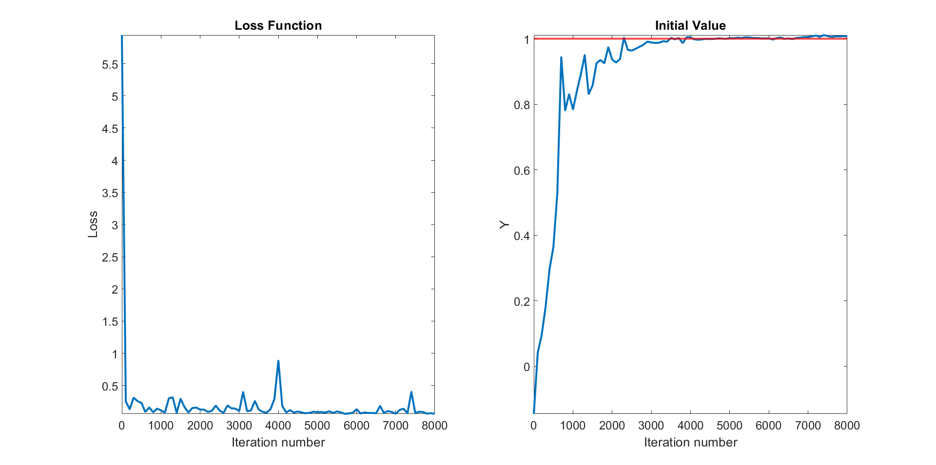
Figure 1. The loss function value (left) and the fitted initial value $X_{0}$ (right) increasing the iteration number for the pure jump expectation example. In red the theoretical value $X_{0}=1$.

The loss function decreases very quickly and the fitted $X_{0}$ reaches a good approximation after only $2000$ iterations. At the end, the initial value obtained using the proposed approach is very close to the theoretical one, showing an error of 0.76%.

5.2. Call option example

Let $X$ denote the price of an underlying asset under the risk-neutral probability measure $\mathbb{Q}$ described by the following dynamics

(5.8) $$\frac{\mathrm{d}X_{t}}{X_{t-}}=r\mathrm{d}t+\sigma\mathrm{d}W^{\mathbb{Q}}_{t}+\int_{\mathbb{R}}(e^{z}-1)\tilde{N}(\mathrm{d}z,\mathrm{d}t)\;,\quad X_{0}=x_{0}\in\mathbb{R},$$

where $r\in\mathbb{R}$, $\sigma\in\mathbb{R^{+}}$ and $\nu(\mathrm{d}z)=\lambda\varphi(z)\mathrm{d}z$ is the Lévy measure with $\lambda>0$ and $\varphi(z)=\frac{1}{\sqrt{2\pi}\sigma_{J}}e^{-\frac{1}{2}\left(\frac{z-\mu_{J}}{\sigma_{J}}\right)^{2}}$.

The solution to (5.8) is given by:

$$X_{T} =X_{t}\exp\left\{\left(r-\frac{\sigma^{2}}{2}\right)(T-t)+\sigma W_{t}^{\mathbb{Q}}-\int_{\mathbb{R}}(e^{z}-1-z)\nu(\mathrm{d}z)(T-t)+\int_{t}^{T}\int_{\mathbb{R}}z\tilde{N}(\mathrm{d}z,\mathrm{d}s)\right\}\;.$$

Let $Y$ be a European call option on $X$ with value at time $t\in[0,T]$ given by

$$Y_{t}=\mathbb{E}^{\mathbb{Q}}\left[e^{-r(T-t)}(X_{T}-k)^{+}|\mathcal{F}_{t}\right]\;,$$

where $k\in\mathbb{R^{+}}$ is the strike price and $(x)^{+}=\max(x,0)$. Thanks to the Markov property of the process $X$ we can write $Y_{t}=u(t,X_{t})$, where $u$ solves the following PIDE:

$$\begin{cases}u_{t}(t,x)+u_{x}(t,x)rx+\frac{1}{2}\sigma^{2}x^{2}u_{xx}(t,x)+\int_{\mathbb{R}}u(t,xe^{z})-u(t,x)-x(e^{z}-1)u_{x}(t,x)\nu(\mathrm{d}z)-ru(t,x)=0\\ u(T,x)=(x-k)^{+}\;.\end{cases}$$

Therefore, the related BSDE is

$$\begin{cases}-\mathrm{d}Y_{s}=-rY_{s}\mathrm{d}s-Z_{s}\mathrm{d}W_{s}^{\mathbb{Q}}-\int_{\mathbb{R}}U(s,z)\tilde{N}(\mathrm{d}z,\mathrm{d}s)\\ Y_{T}=(X_{T}-k)^{+}\;,\end{cases}$$

where, from the Feynman-Kac representation formula we also have $Z_{t}=u_{x}(t,X_{t^{-}})\sigma X_{t^{-}}$ and $U_{t}(z)=u(t,X_{t^{-}}e^{z})-u(t,X_{t^{-}})$.

Our goal is to estimate the value $Y_{0}$ using the deep solver and compare it with a standard Monte Carlo simulation. We set $X_{0}=1$, $k=0.9$, $r=0.04$, $\sigma=0.25$, $\lambda=0.3$, $\mu_{J}=0.5$, $\sigma_{J}=0.25$. For the numerical scheme, we use $M=40$ time steps and $8000$ iterations for the optimization for ANNs with $2$ hidden layers each one with $\upsilon=d+1=21$ nodes. The batch size is equal to 64. The deep solver results are reported in Table 13 and Figure 5 while the Monte Carlo result is $Y_{0}^{mc}=0.251$.

Table 3. Algorithm results for the call option example.

Step	Loss	$Y_{0}$	Time∗
0	15.738	0.017	36
100	0.513	0.056	156
500	0.281	0.084	195
1000	0.108	0.182	243
2000	0.082	0.247	341
3000	0.162	0.252	439
4000	0.197	0.258	536
5000	0.127	0.254	629
6000	0.107	0.253	725
7000	0.106	0.250	827
8000	0.097	0.250	927

Table 4. *

^∗ Elapsed time in seconds

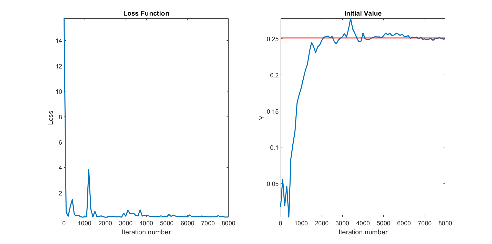
Figure 2. The loss function value (left) and the fitted initial value $Y_{0}$ (right) increasing the iteration number for the call option example. In red the Monte Carlo fitted value $Y_{0}^{mc}=0.251$

As in the previous case, the loss function decreases rapidly and the fitted $Y_{0}$ provides a good approximation after only $2000$ iterations. Finally, the initial valued obtained using the deep solver is very close to the value resulting from Monte Carlo approach; the error is only $0.46\%$.

5.3. A Basket call option example

The examples we presented so far are mainly meant to provide a validation of the methodology in the one dimensional case. The example we proceed to discuss now instead provides evidence that the methodology is viable in a high dimensional setting. We consider the case of several underlying assets $(X^{1};\cdots;X^{d})$:

(5.9) $$\frac{\mathrm{d}X_{t}^{i}}{X_{t-}^{i}}=r^{i}\mathrm{d}t+\sigma^{i}\mathrm{d}W^{\mathbb{Q},i}+\int_{\mathbb{R}}(e^{z}-1)\tilde{N}^{i}(\mathrm{d}z,\mathrm{d}t)\;,\quad X_{0}^{i}=x_{0}^{i}\in\mathbb{R}^{d},\quad i=1,\cdots,d\,,$$

where $r^{i}\in\mathbb{R}$, $\sigma^{i}\in\mathbb{R^{+}},i=1,\cdots,d$, $W^{\mathbb{Q}}=(W^{\mathbb{Q},1},\cdots,W^{\mathbb{Q},d})$ is a standard Brownian motion in $\mathbb{R}^{d}$ and $\nu^{i}(\mathrm{d}z)=\lambda\varphi(z)\mathrm{d}z$, $i=1,\cdots,d$, is the Lévy measure with $\lambda>0$ and $\varphi(z)=\frac{1}{\sqrt{2\pi}\sigma_{J}}e^{-\frac{1}{2}\left(\frac{z-\mu_{J}}{\sigma_{J}}\right)^{2}}$.

The solution to (5.9) satisfies, for any $i=1,\ldots,d$,

$$\begin{aligned} X_{T}^{i}=X_{t}^{i}\exp\left\{\left(r^{i}-\frac{\sigma^{2,i}}{2}\right)(T-t)+\sigma^{i}W_{t}^{\mathbb{Q},i}-\int_{\mathbb{R}}(e^{z}-1-z)\nu^{i}(\mathrm{d}z)(T-t)+\int_{t}^{T}\int_{\mathbb{R}}z\tilde{N}^{i}(\mathrm{d}z,\mathrm{d}s)\right\}\;.\end{aligned}$$

Let $Y$ be a basket of European call option on $(X^{1};\cdots;X^{d})$ with value at time $t\in[0,T]$ given by

(5.10) $$Y_{t}=\mathbb{E}^{\mathbb{Q}}\left[e^{-r(T-t)}\left(\sum_{i=1}^{d}X_{T}^{i}-d\,k\right)^{+}\biggr{|}\mathcal{F}_{t}\right]\;.$$

where $k\in\mathbb{R^{+}}$ is the strike price. From the Feynman-Kac representation formula we have $Y_{t}=u(t,X_{t}^{1},\cdots,X_{t}^{d})=u(t,X_{t})$ where $u$ solves the following PIDE:

(5.11) $$\begin{cases}\!\begin{aligned} u_{t}(t,x)+\nabla_{x}u(t,x)b_{x}+\frac{1}{2}\mathop{\mathrm{Tr}}\left[\sigma\sigma^{\intercal}(t,x)D^{2}_{x}u(t,x)\right]&-ru(t,x)\\ +\int_{\mathbb{R}^{d}}u(t,x_{.}e^{z})-u(t,x)&-x_{.}(e^{z}-\mathbf{1})\nabla_{x}u(t,x)\nu(\mathrm{d}z)=0\end{aligned}\\ u(T,x)=\left(\sum_{i=1}^{d}x_{i}-d\,k\right)^{+};\end{cases}$$

where we use _. to denote the component-wise product between vectors, $e^{z}$ is the vector where each entry is of the form $e^{z_{i}}$, $i=1,\ldots d$, $\mathbf{1}$ is the vector with all elements equal to one and $\nu$ is the product of the $d$ Lévy measures of the individual driving processes. Therefore, the related BSDE is

(5.12) $$\begin{cases}-\mathrm{d}Y_{s}=-rY_{s}\mathrm{d}s-Z_{s}\mathrm{d}W_{s}^{\mathbb{Q}}-\int_{\mathbb{R}^{d}}U(s,z)\tilde{N}(\mathrm{d}z,\mathrm{d}s)\\ Y_{T}=\left(\sum_{i=1}^{d}X_{T}^{i}-d\,k\right)^{+};,\end{cases}$$

where $U_{t}(z)=u(t,X_{t^{-}}{}_{.}e^{z})-u(t,X_{t^{-}})$.

Once again, we estimate the value $Y_{0}$ using the deep solver and compare it with a standard Monte Carlo simulations. We set $d=100$, $X_{0}=\mathbf{1}$, ${k=0.9};r=0.04;\sigma^{i}=\sigma=0.25$ for all $i=1,\cdots,d$, $\lambda=0.3$, $\mu_{J}=0.5$, $\sigma_{J}=0.25$. We consider $M=40$ time steps and perform $20.000$ iterations, with ANNs with $\mathcal{L}-1=2$ hidden layers each with $\upsilon=d+20=120$ nodes. The batch size is maintained equal to $64$. We have increased the iterations number compared to the previous examples to have more accurate estimates as the problem dimension increases. The deep solver results are reported in Table 6 and Figure 3 while the Monte Carlo result is $Y_{0}^{mc}=13.607$.

Table 5. Algorithm results for a basket call option example of dimension $100$.

Step	Loss	$Y_{0}$	Time∗
0	274.500	-0.068	57
100	40.219	1.590	242
1000	31.378	12.241	444
2000	23.488	12.820	648
3000	35.340	11.852	854
4000	25.627	12.367	1065
5000	21.274	12.493	1270
8000	29.688	13.299	1900
10000	20.917	13.028	2319
15000	18.102	13.510	3372
20000	17.951	13.479	4438

Table 6. *

^∗ Elapsed time in seconds

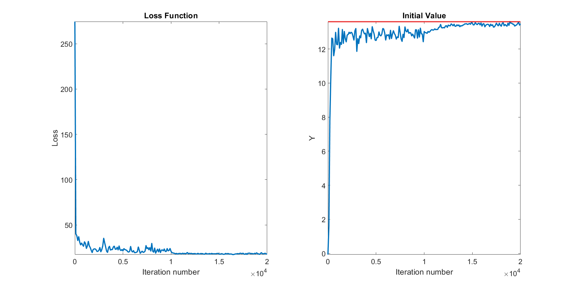
Figure 3. The loss function value (left) and the fitted initial value $Y_{0}$ (right) increasing the iteration number for the basket call option example of dimension 100. In red the Monte Carlo fitted value $Y_{0}^{mc}=13.607$

In spite of the high dimension of the problem, also in this case, the loss function decreases quite fast and the fitted $Y_{0}$ reaches a good approximation after only $2000$ iterations. At the end, the initial valued obtained using the deep solver is very close to the value resulting from the Monte Carlo approach showing an error of 0.95%. The estimation procedure requires about 74 minutes to perform $20.000$ iterations. Comparing the elapsed time at $8000$ iterations as in the previous cases, we note that we can obtain good results in $d=100$ with only twice as much computational time.

5.3.1. Robustness checks

It may be argued that the goodness of estimates could be affected by a specific set of parameters. In order to address such type of questions we propose a set of robustness checks. At first, we run the algorithm on the basket call example by varying the dimension of the problem. In Table 8 we show the results which display an error lower than 1% in all cases.

Table 7. Simulations results by varying basket dimension.

Dim	MC Price	BSDE Price	Err.%	Time∗
5	0.903	0.908	0.59%	1984
10	1.614	1.612	0.15%	1861
25	3.618	3.612	0.17%	2105
50	6.858	6.902	0.64%	2450
75	10.138	10.093	0.44%	2840
100	13.607	13.479	0.95%	4438

Table 8. *

^∗ Elapsed time in seconds

It is important to note that by increasing the number of time steps, the proposed procedure implies a substantial growth in the number of parameters to be estimated, since each additional time step implies the introduction of two additional neural networks whose parameters need to be estimated. For this reason, as the number of time steps increases, it could be necessary to increase the number of iterations of the optimizer. This is shown in Table 10: moving from $20000$ to $40000$ iterations, we can reduce the error of the procedure from $7.01\%$ to $0.03\%$.

Table 9. Simulation results by varying iterations number.

Iter.	MC Price	BSDE Price	Err.%	Time∗
20,000	13.645	12.751	7.01%	10231
40,000	13.528	13.524	0.03%	20274

Table 10. *

^∗ Elapsed time in seconds

Finally, we control for the intensity jump parameter $\lambda$, see Table 11. The intuition behind the experiment is the following: if the jump intensity/activity is high, a finer time discretization grid will be needed in order to realistically approximate the trajectories of the FBSDE. As expected, we find that the error substantially increases when $\lambda$ increases, thus signaling the need to introduce a finer time discretization. We remark however that the values of $\lambda$ we are employing in the present experiment are much higher in comparison to those obtained from a calibration to prices of financial products, see among others Kienitz and Wetterau (2013).

Table 11. Simulation results by varying $\lambda$.

$\lambda$	MC Price	BSDE Price	Err.%
0.1	13.515	13.505	0.08%
0.3	13.607	13.479	0.95%
0.5	13.772	13.602	1.25%
0.7	14.019	13.839	1.30%
0.9	14.524	14.085	3.12%
1.1	14.944	14.263	4.78%
1.3	16.111	14.457	11.44%

5.4. Infinite activity example

The final example we propose provides evidence for the feasibility of the proposed algorithm for the infinite activity case. We consider the CGMY process, which is a pure jump Lévy process $L$ with characteristic triplet $(0,0,\nu(\mathrm{d}z))$, where the Lévy measure is given by

$$\nu(\mathrm{d}z)=C\frac{e^{-G|z|}}{|z|^{1+Y}}\mathtt{1}_{\{z<0\}}\mathrm{d}z+C\frac{e^{-Mz}}{z^{1+Y}}\mathtt{1}_{\{z>0\}}\mathrm{d}z.$$

The Lévy measure corresponds to that of a difference of two tempered stable subordinators, meaning that we can write $L_{t}=L^{+}_{t}-L^{-}_{t}$ where

• $L^{+}$ has triplet $(0,0,\nu^{+}(\mathrm{d}z))$, where $\nu^{+}(\mathrm{d}z):=C\frac{e^{-Mz}}{z^{1+Y}}\mathtt{1}_{\{z>0\}}\mathrm{d}z$;

• $L^{-}$ has triplet $(0,0,\nu^{-}(\mathrm{d}z))$, where $\nu^{-}(\mathrm{d}z):=C\frac{e^{-Gz}}{z^{1+Y}}\mathtt{1}_{\{z>0\}}\mathrm{d}z$.

In the following we outline the procedure to approximate a tempered stable subordinator by following Cont and Tankov (2003) and references therein among others. Since the procedure is the same for $L^{+}$ and $L^{-}$, we choose to concentrate on $L^{+}$. We fix $\epsilon>0$: this will represent a threshold for jump sizes: all jumps smaller than $\epsilon$ will be approximated by a diffusion process, whereas all jumps larger than $\epsilon$ will be approximated by a suitably constructed compensated compound Poisson process. We first look at the large jumps. The jump compensator of the approximating compound Poisson process is given by

$$\int_{\epsilon}^{\infty}zC\frac{e^{-Mz}}{z^{1+Y}}\mathrm{d}z =C\int_{\epsilon}^{\infty}z^{-Y}e^{-Mz}\mathrm{d}z=C\int_{M\epsilon}^{\infty}\left(\frac{\ell}{M}\right)^{-Y}e^{-\ell}\mathrm{d}\ell$$

$$=\frac{C}{M^{a}}\int_{M\epsilon}^{\infty}\ell^{a-1}e^{-\ell}\mathrm{d}\ell\;,$$

where we set $a:=1-Y$. Let us now recall the lower incomplete Gamma function as implemented in scipy or Matlab $\Gamma(a,M\epsilon):=\frac{1}{\Gamma(a)}\int_{0}^{M\epsilon}\ell^{a-1}e^{-\ell}\mathrm{d}\ell$, where $\Gamma(a)$ is the Gamma function computed in $a$. We conclude that

$$\int_{\epsilon}^{\infty}zC\frac{e^{-Mz}}{z^{1+Y}}\mathrm{d}z =\Gamma(a)\left(1-\Gamma(a,M\epsilon)\right):=-b_{\epsilon^{+}}\;.$$

The intensity of the approximating compound Poisson process is given by

$$\lambda^{+}_{\epsilon}:=\int_{\epsilon}^{\infty}C\frac{e^{-Mz}}{z^{1+Y}}\mathrm{d}z\;.$$

To find a convenient expression for the intensity, we integrate by parts and obtain

$$\int_{0}^{\infty}zC\frac{e^{-Mz}}{z^{1+Y}}\mathrm{d}z=\frac{C}{M}e^{-M\epsilon}\epsilon^{-Y}-\frac{YC}{M}\int_{\epsilon}^{\infty}e^{-Mz}z^{-1-Y}\mathrm{d}z\;.$$

By rearranging terms, we can write

$$\lambda^{+}_{\epsilon}=Ce^{-M\epsilon}\frac{\epsilon^{-Y}}{Y}+\frac{M}{Y}b_{\epsilon^{+}}\;.$$

Next, we need to determine the jump size distribution. We denote by $f_{\epsilon^{+}}$ such density. Recalling the general form of the Lévy measure of a compound Poisson process we can write

$$f_{\epsilon^{+}}(z)=\frac{1}{\lambda^{+}_{\epsilon}}C\frac{e^{-Mz}}{z^{1+Y}}\mathtt{1}_{\{z>\epsilon\}}\;.$$

It is possible to sample from such distribution by means of the acceptance rejection method as outlined in Cont and Tankov (2003). Finally, we also introduce a diffusion approximation of small jumps. The coefficient of the diffusion approximation is given by

$$\sigma^{2}_{\epsilon}:=\int_{-\epsilon}^{\epsilon}z^{2}\nu(\mathrm{d}z)\;.$$

Again, due to the particular structure of the Lévy measure, we can split the computation between the positive and negative jumps. For the positive jumps we have

$$\int_{0}^{\epsilon}z^{2}C\frac{e^{-Mz}}{z^{1+Y}}\mathrm{d}z=\frac{C}{M^{2-Y}}\Gamma(a+1)\Gamma(a+1,M\epsilon)\;,$$

and similarly for the negative jumps. In summary, to simulate the CGMY process $L$, we introduce the discrete time approximation $L^{\epsilon}$ given by

$$L^{\epsilon}_{t_{n+1}}=L^{\epsilon}_{t_{n}}+\sigma_{\epsilon}\Delta W_{n+1}+\sum_{j=1}^{N_{n+1}^{+}}\Delta L_{n+1,j}^{+}-b_{\epsilon^{+}}\Delta_{n+1}-\sum_{j=1}^{N_{n+1}^{-}}\Delta L_{n+1,j}^{-}+b_{\epsilon^{-}}\Delta_{n+1}\;,$$

where

$$N_{n+1}^{+} \sim\mathcal{P}\left(\lambda_{\epsilon}^{+},\Delta_{n+1}\right)\;,$$

$$N_{n+1}^{-} \sim\mathcal{P}\left(\lambda_{\epsilon}^{-},\Delta_{n+1}\right)\;,$$

$$\Delta L_{n+1,j}^{+} \sim f_{\epsilon^{+}}\;,$$

$$\Delta L_{n+1,j}^{-} \sim f_{\epsilon^{-}}\;.$$

The approximating asset price process is then of the form

(5.13) $$X^{\epsilon}_{t_{n+1}}=X^{\epsilon}_{t_{n}}\exp\left\{-\int_{\mathbb{R}}(e^{z}-1-z)\nu(\mathrm{d}z)(t_{n+1}-t_{n})+L^{\epsilon}_{t_{n+1}}-L^{\epsilon}_{t_{n}}\right\}\;,\\$$

where

$$-\int_{\mathbb{R}}(e^{z}-1-z)\nu(\mathrm{d}z)=-C\Gamma(-Y)\left((M-1)^{Y}-M^{Y}+(G+1)^{Y}-G^{Y}\right)\;.$$

5.4.1. Call option under the CGMY model

Let $X$ be the price of a stock described by (5.13) and $Y$ a European call option with value

(5.14) $$Y_{t}=\mathbb{E}^{\mathbb{Q}}\left[e^{-r(T-t)}(X_{T}-k)^{+}|\mathcal{F}_{t}\right].$$

Our goal is to estimate the value $Y_{0}$ using the deep solver and compare it with a standard Monte Carlo simulations. Before we proceed with the estimation, we test the goodness of fit of the proposed approximation by comparing it with the semi closed-form density obtained via the Fast Fourier Transform (FFT) applied to the characteristic function of the CGMY process. In Figure 4 we are able to verify the goodness of fit.

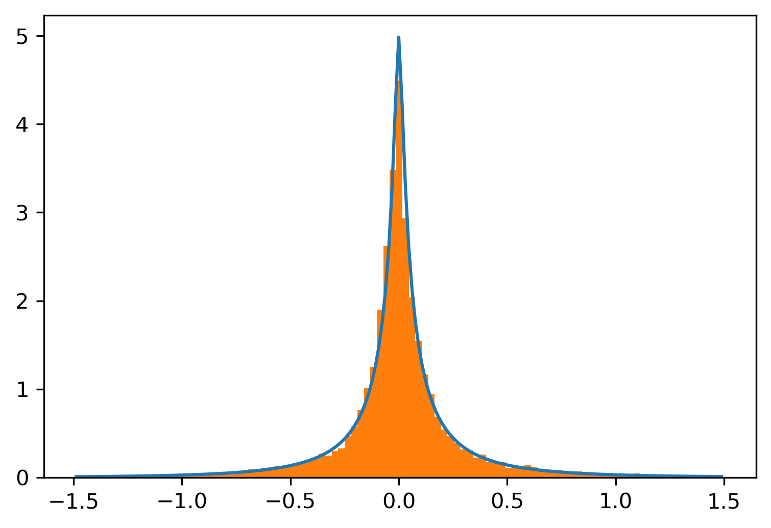
Figure 4. Histogram of empirical density in orange and true density in blue.

We set $X_{0}=1$, $k=0.9$, $r=0.04$, $C=0.1$, $G=1.4$, $M=1.3$, $Y=0.5$, $\epsilon=0.0001$. We consider $M=100$ time steps, $8000$ iterations and the same ANNs’ architecture of the previous examples. The deep solver results are reported in Table 13 and Figure 5 while the Monte Carlo result is $Y_{0}^{mc}=0.164$.

Table 12. Algorithm results for the call option with CGMY example.

step	loss	$Y_{0}$	Time∗
0	54.462	0.518	127
100	0.212	0.494	519
500	0.442	0.428	666
1000	0.148	0.353	845
2000	0.248	0.289	1211
3000	0.459	0.140	1586
4000	2.991	0.141	1948
5000	0.023	0.140	2304
6000	0.085	0.162	2652
7000	0.032	0.158	2999
8000	0.019	0.161	3363

Table 13. *

^∗ Elapsed time in seconds

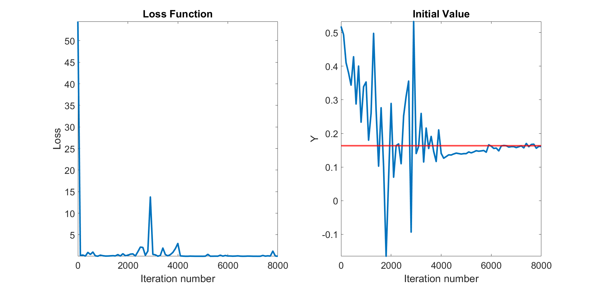
Figure 5. The loss function value (left) and the fitted initial value $Y_{0}$ (right) increasing the iteration number for the call option example. In red the Monte Carlo fitted value $Y_{0}^{mc}=0.164$

The loss function varies significantly during the first 2500 iterations and then stabilizes during the subsequent 2500 iterations: this is due to the choice of a schedule for the learning rate. The fitted $Y_{0}$ reaches a good approximation after $3000$ iterations. At the end, the initial value obtained by using the deep solver is very close to the value resulting from the Monte Carlo approach, showing an error of $1.72\%$. However, in this case, the elapsed time for the fitting is greater and takes about 56 minutes: the increase in the computational time is due to the procedure that constructs the approximating Poisson processes.

References

- Al-Aradi et al. (2019) Al-Aradi, A., Correia, A., de Frietas Naiff, D., Jardim, G., and Saporito, Y. (2019). Extensions of the Deep Galerkin Method. arXiv e-prints, page arXiv:1912.01455.
- Applebaum (2009) Applebaum, D. (2009). Lévy Processes and Stochastic Calculus, volume 116 of Cambridge Studies in Advanced Mathematics. Cambridge University Press, second edition.
- Asmussen and Rosiński (2001) Asmussen, S. and Rosiński, J. (2001). Approximations of small jumps of lévy processes with a view towards simulation. Journal of Applied Probability, 38(2):482–493.
- Beck et al. (2021) Beck, C., Becker, S., Cheridito, P., Jentzen, A., and Neufeld, A. (2021). Deep splitting method for parabolic pdes. SIAM Journal on Scientific Computing, 43(5):A3135–A3154.
- Castro (2021) Castro, J. (2021). Deep Learning Schemes For Parabolic Nonlocal Integro-Differential Equations. arXiv e-prints, page arXiv:2103.15008.
- Cohen and Rosiński (2007) Cohen, S. and Rosiński, J. (2007). Gaussian approximation of multivariate Lévy processes with applications to simulation of tempered stable processes. Bernoulli, 13(1):195 – 210.
- Cont and Tankov (2003) Cont, R. and Tankov, P. (2003). Financial Modelling with Jump Processes. Chapman & Hall/CRC.
- Cybenko (1989) Cybenko, G. (1989). Approximations by superpositions of sigmoidal functions. Mathemtics of Control, Signals, and Systems, 2(4):303–314.
- Delong (2017) Delong, L. (2017). Backward Stochastic Differential Equations with Jumps and Their Actuarial and Financial Applications. Springer, Berlin, New York.
- E et al. (2017) E, W., Han, J., and Jentzen, A. (2017). Deep learning-based numerical methods for high-dimensional parabolic partial differential equations and backward stochastic differential equations. Communications in Mathematics and Statistics, 5:349–380.
- Fournier (2011) Fournier, N. (2011). Simulation and approximation of lévy-driven stochastic differential equations. ESAIM: Probability and Statistics, 15:233–248.
- Frey and Köck (2021) Frey, R. and Köck, V. (2021). Deep Neural Network Algorithms for Parabolic PIDEs and Applications in Insurance Mathematics. arXiv e-prints, page arXiv:2109.11403.
- Frey and Köck (2022) Frey, R. and Köck, V. (2022). Convergence Analysis of the Deep Splitting Scheme: the Case of Partial Integro-Differential Equations and the associated FBSDEs with Jumps. arXiv e-prints, page arXiv:2206.01597.
- Han et al. (2018) Han, J., Jentzen, A., and E, W. (2018). Solving high-dimensional partial differential equations using deep learning. Proceedings of the National Academy of Sciences, 115(34):8505–8510.
- Han and Long (2020) Han, J. and Long, J. (2020). Convergence of the deep BSDE method for coupled FBSDEs. Probability, Uncertainty and Quantitative Risk, 5(1):1–33.
- Hilber et al. (2013) Hilber, N., Reichmann, O., Schwab, C., and Winter, C. (2013). Computational methods for quantitative finance. Springer Finance. Springer, Berlin, Germany, 2013 edition.
- Hornik (1991) Hornik, K. (1991). Approximation capabilities of multilayer feedforward networks. Neural Networks, 4(2):251–257.
- Huré et al. (2020) Huré, C., Pham, H., and Warin, X. (2020). Deep backward schemes for high-dimensional nonlinear pdes. Mathematics of Computation, 89(324):1547–1579.
- Hutzenthaler et al. (2018) Hutzenthaler, M., Jentzen, A., Kruse, T., Nguyen, T. A., and von Wurstemberger, P. (2018). Overcoming the curse of dimensionality in the numerical approximation of semilinear parabolic partial differential equations. arXiv preprint arXiv:1807.01212.
- Jacod and Shiryaev (2003) Jacod, J. and Shiryaev, A. (2003). Limit Theorems for Stochastic Processes, volume 288 of Grundlehren der mathematischen Wissenschaften. Springer, Berlin - Heidelberg - New York, second edition.
- Jentzen et al. (2018) Jentzen, A., Salimova, D., and Welti, T. (2018). A proof that deep artificial neural networks overcome the curse of dimensionality in the numerical approximation of Kolmogorov partial differential equations with constant diffusion and nonlinear drift coefficients. arXiv preprint arXiv:1809.07321.
- Jum (2015) Jum, E. (2015). Numerical Approximation of Stochastic Differential Equations Driven by Levy Motion with Infinitely Many Jumps. PhD thesis, University of Tennessee.
- Kienitz and Wetterau (2013) Kienitz, J. and Wetterau, D. (2013). Financial modelling: Theory, implementation and practice with MATLAB source. John Wiley & Sons.
- Kingma and Ba (2015) Kingma, D. P. and Ba, J. (2015). Adam: A Method for Stochastic Optimization. In Proceedings of the 3rd International Conference for Learning Representations, San Diego, 2015.
- Kolmogorov (1956) Kolmogorov, A. N. (1956). On the representation of continuous functions of several variables by superposition of continuous functions of one variable and addition. Doklady Akademii Nauk SSSR, 108(2):679–681.
- Kunita (2004) Kunita, H. (2004). Stochastic differential equations based on lévy processes and stochastic flows of diffeomorphisms. In Real and Stochastic Analysis, pages 305–373. Birkhäuser Boston, Boston, MA.
- Reisinger and Zhang (2020) Reisinger, C. and Zhang, Y. (2020). Rectified deep neural networks overcome the curse of dimensionality for nonsmooth value functions in zero-sum games of nonlinear stiff systems. Analysis and Applications. https://doi.org/10.1142/S0219530520500116.
- Sirignano and Spiliopoulos (2018) Sirignano, J. and Spiliopoulos, K. (2018). Dgm: A deep learning algorithm for solving partial differential equations. Journal of Computational Physics, 375:1339–1364.
- Thomas (1998) Thomas, J. W. (1998). Numerical partial differential equations: Finite difference methods. Texts in Applied Mathematics. Springer, New York, NY, 1 edition.