Calibrated Perception Uncertainty Across Objects and Regions in Bird’s-Eye-View

Abstract

In driving scenarios with poor visibility or occlusions, it is important that the autonomous vehicle would take into account all the uncertainties when making driving decisions, including choice of a safe speed. The grid-based perception outputs, such as occupancy grids, and object-based outputs, such as lists of detected objects, must then be accompanied by well-calibrated uncertainty estimates. We highlight limitations in the state-of-the-art and propose a more complete set of uncertainties to be reported, particularly including undetected-object-ahead probabilities. We suggest a novel way to get these probabilistic outputs from bird’s-eye-view probabilistic semantic segmentation, in the example of the FIERY model. We demonstrate that the obtained probabilities are not calibrated out-of-the-box and propose methods to achieve well-calibrated uncertainties.

1 Introduction

Autonomous vehicles (AVs) are more popular and feasible than ever before, heavily relying on different sensors: LiDARs, radars, GPS, and cameras. With the high travelling speed of the vehicles in the traffic, the planning and decision-making subsystem of AVs must make fast and justified decisions about the driving speed and trajectory, avoiding other vehicles, pedestrians, and obstacles (Koopman, 2022). To ensure safety, reliable and uncertainty-aware outputs are needed from the perception subsystem which has to detect surrounding objects (Veres et al., 2010; Gruyer et al., 2017). Planning and decision-making methods for autonomous driving (AD) are increasingly able to make use of perception uncertainty (Claussmann et al., 2019). To facilitate further improvements in the perception-planning stack, the goal of our paper is to (1) discuss limitations of existing perception uncertainty quantification methods for AD; (2) propose a more complete set of uncertainty estimates; and (3) propose practical methods to obtain uncertainty estimates for this set. In particular, we aim to have uncertainty estimates that are well-calibrated, in the sense that if the model predicts a pedestrian with 80 percent probability for 100 times, then 80 times out of these 100 there should be a pedestrian.

1.1 Related work

There are various methods for motion planning and for creating a representation of driving situation (Claussmann et al., 2019). Many of them are based on finding cost maps (Choset et al., 2005). Cost maps give costs to different paths or trajectories, which can be based on cost functions checking constraints from situations and different obstacles (Kuwata et al., 2009). Cost maps may also consider uncertainty about different aspects, for example, localisation (Gonzalez and Stentz, 2007) and environment (Kuwata et al., 2009). Further, to find suitable paths, occupancy grids can be used (Mouhagir et al., 2016). Occupancy grids are divided into cells, denoting where detected objects are. For example, Voronoi uncertainty fields (Ok et al., 2013) and occupancy grids with safety distances (Mouhagir et al., 2016) are using uncertainty to avoid collisions in finding plausible trajectories.

While the grid-based view using cost maps or occupancy grids provides useful information about each location, it lacks the object-specific information which is important for behavioural modelling (Claussmann et al., 2019). Therefore, it is important to explicitly detect individual objects, and identify their location, class, etc, which we refer to as the object-based view. For example, YOLOv3 (Redmon and Farhadi, 2018) outputs bounding boxes for each object in the image. Further using Gaussian YOLOv3 (Choi et al., 2019), uncertainties about bounding box location are modeled as well. However, 2D bounding boxes lack distance information, which is available in 3D bounding boxes (Yang et al., 2019).

Due to the computational limitations, the list of detected objects in the object-based view always remains non-exhaustive, in the sense that there can be objects that are not detected by the object-based view, while the grid-based view still shows some tiny probability (e.g. less than one-in-a-million) for something to be present at that location. Ignoring such objects is hazardous and not acceptable, e.g. consider driving in fog. Therefore, the information from the grid-based and object-based views is complementary, and it is preferable if the perception system can provide both. To some extent, the object-based view can be extracted from several grid-based views, as it has been done in the FIERY model (Hu et al., 2021).

FIERY (Hu et al., 2021) is a bird’s-eye-view (BEV) semantic segmentation model. FIERY converts surrounding camera images into top-down semantic segmentation of vehicles. It takes six camera images and intrinsic and extrinsic information about cameras as input. FIERY uses past time steps and current time steps to output semantic segmentation for current and future time steps. Further, to achieve instance segmentation with trajectories, FIERY has the following four outputs: semantic segmentation, offset, flow and centerness, which are all grid-based, with the resolution of 0.5m x 0.5m grid cells. By combining these outputs and by using thresholding and clustering it is possible to extract object-based information, e.g. in the form of instance segmentation which differentiates individual vehicles or pedestrians, in contrast to the standard segmentation which for any grid cell only provides the class (vehicle, pedestrian, etc.).

The grid-based view is typically readily providing individual uncertainty estimates for each grid cell, e.g. in FIERY the semantic segmentation is probabilistic, for each cell providing the probability of whether an object is covering this cell or not. The object-based view as in YOLOv3 can include objectness scores (Choi et al., 2019) where a higher score stands for a higher probability to be a true positive, whereas a lower score is more likely to indicate a false positive.

For safety, it is very important to be able to calculate the probability that the road ahead is safe to drive in the sense that there are no other vehicles, pedestrians or obstacles other than those already detected by the perception system (Koopman, 2022). Such probability is essential for deciding about safe driving speed. For example, in case of poor visibility due to weather or lighting conditions it is more likely that some objects have not been detected. However, to our knowledge, the existing perception systems do not provide such undetected-object-ahead probability explicitly.

1.2 Contributions

• We propose a more complete set of outputs that the perception subsystem needs to provide to the planning and decision-making subsystem, including undetected-object-ahead probabilities;

• We suggest a novel way to get these probabilistic outputs from bird’s-eye-view (BEV) probabilistic semantic segmentation;

• We show that these outputs are not calibrated out-of-the-box and propose methods to achieve well-calibrated uncertainty estimates also.

The out-of-distribution aspect of uncertainty quantification (Amodei et al., 2016) remains out of the scope of this paper and is an important future research direction.

2 Uncertainty-aware perception for autonomous driving

This section gives an overview of our approach to uncertainty-aware perception for autonomous driving. The potential need and benefits of such an approach are described and explained.

2.1 Envisioned role of uncertainty in the perception-planning stack

The role of uncertainty is growing more and more in perception-planning; however, the planning algorithms have not yet fully adapted it (Section 1.1). Thus, we propose to use extra uncertainty information about detected and undetected objects.

Following our proposal, the perception model should report:

1. a list of detected objects, and for each of these objects: (a) presence uncertainty, i.e. the probability that this is actually an object and not a false positive detection; (b) location uncertainty, i.e. a probability distribution over possible locations of the mass centre of this object; (c) shape uncertainty, i.e. a probability distribution over possible shapes (including orientations) of this object; (d) trajectory uncertainty, i.e. a probability distribution over possible trajectories that this object would take in the near future;

2. undetected-object-ahead uncertainties for several relevant regions (e.g. at different distances, or e.g. current lane, and lanes to the left and right), providing for each such region a single probability that there is an undetected object in that region.

To make this proposal clearer, let us consider an example, where the FIERY model trained for detecting pedestrians (see details below in the Experiments). This model provides a bird’s-eye-view (BEV) probabilistic semantic segmentation with 0.5m x 0.5m grid cells, see Figure 1(a), where the colours indicate log-scale probabilities for the grid cell to contain an object, and the ego-vehicle is located at $(100,100)$. Due to limited computational resources in the perception-planning stack, the object-based view cannot contain all the positive signals from the grid-based view, visualised by clipping at $-5$ in subfigure (b). Subfigure (c) illustrates location uncertainty of the detected (above threshold) objects (ellipsoids) as well as example regions (red rectangles) ahead of the ego-vehicle (blue rectangle) for which our approach can provide undetected-object-ahead probabilities, one for each region.

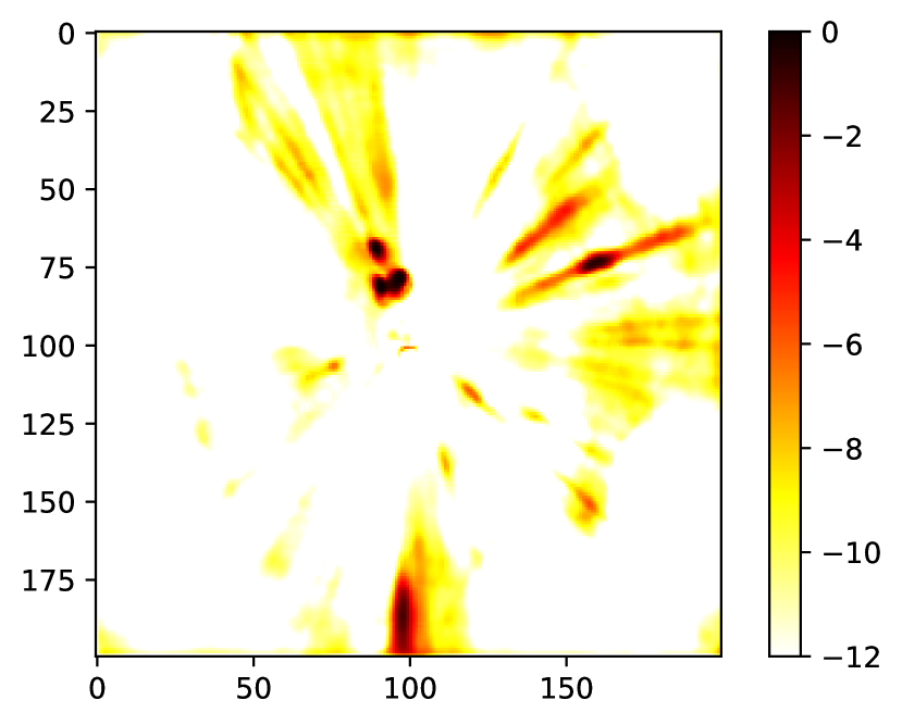
(a)

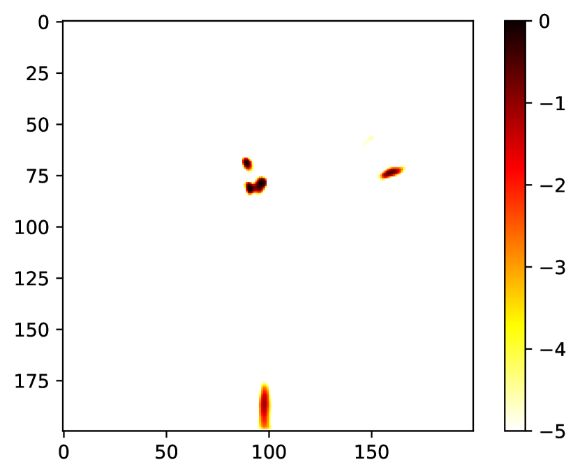
(b)

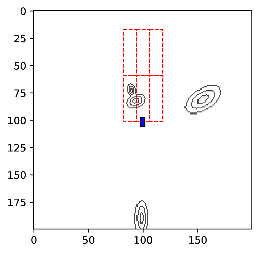
(c)

Figure 1: BEV perception uncertainty on top of the FIERY model. Subfigures (a) and (b) display FIERY semantic segmentation in log-scale (natural logarithm) for better visibility, clipped at -12 in (a) and at -5 in (b). Subfigure (c) shows our proposed extra information about locations (ellipsoids) and undetected areas (dashed red rectangles). The blue rectangle at $(100,100)$ indicates the ego-vehicle. The example is generated using approach in Section 2.2

In the following paragraphs, we describe the need for different extra inputs to the planner (i.e. outputs from perception) and their potential benefits compared to planners using only segmentation or detected objects.

The need of probabilistic object presence.

The planner of course needs to come up with a trajectory avoiding all detected objects. However, it can sometimes happen that it is no longer physically possible to obtain a 100% safe trajectory avoiding all objects, and then it becomes important which detected objects are more likely to be false detections.

The need of probabilistic object center location.

It is used by the planner to reason about the uncertainties of where is the predicted object. The location uncertainties give information on how confident the model is about the object’s location, and the planner must avoid any possible collisions caused by bad localization.

The need of probabilistic object shape.

It is used to consider the possible variability of an object’s dimensions and shape. The object’s shape is needed for the planner to reason about the object’s possible position and how much area it might take. The higher shape uncertainty could mean that the object is occluded, or the conditions make it harder for the model to predict precise shape.

The need of probabilistic trajectory of the objects.

These are needed for the planner to reason about the future location of dynamic objects and find out about static objects. These uncertainties are required to predict other participants’ behaviors in traffic. If the behavior of other participants is uncertain, the planner should take extra caution.

The need of the undetected-object-ahead probabilities by areas.

These are needed for the planner to reason about the risk of missing an object and the safe speed to continue driving. These areas give extra information about how likely it is in an area to find missed objects and what areas should be avoided or when it is necessary to slow down because of significant uncertainty.

The first three, the location and presence probability with shape, are needed to achieve complete information about a detected object. This kind of split helps to understand the possible size and location of the object. For example, if the shape is known, it is possible to assume how much area it takes in location prediction. This information can also be used to select the best trajectory to avoid the object potentially. For example, if the model output that the object is more towards left than right, the planner could also consider choosing the best trajectory, as if the object is in one location, it cannot be in another. And when getting closer, the planner receives more information from the model about the object’s location.

All these inputs should be well-calibrated to reflect the truth about different driving scenarios and conditions. Further, these inputs can be used to assess risk and check model reliability.

2.2 Methodology

In this subsection, we propose methodology of how the previously mentioned five outputs (object presence, object location, object shape, object trajectory, and undetected object presence) can be extracted from probabilistic BEV semantic segmentation, and how the uncertainty estimates can be calibrated. BEV semantic segmentation has been previously used by some planners as an input (Paden et al., 2016) and we believe that our extended set of perception outputs and associated well-calibrated uncertainties can be used to improve the performance of the perception-planning stack further.

The probabilistic object center location.

This probability distribution $d_{loc}$ can be modeled as, for example, a two-dimensional (2D) Gaussian, for x and y coordinates in BEV. The location uncertainty from semantic segmentation can be fitted with Gaussian mixture models (GMM) with one Gaussian per object.

First, a suitable number of GMM nodes are selected by finding potential cluster centers based on semantic segmentation and with a probability threshold of $p_{thresh}$. For this we use the same clustering method as used in the FIERY model uses for obtaining instance segmentation (Hu et al., 2021). Next, we sample with replacement a large set of possible object locations following the probabilities in individual grid-cells, i.e. grid-cells with high segmentation probability will give rise to many points and grid-cells with low probability yield no points at all. GMM is then fitted on this set of possible object locations. In practice, we use stratified sampling in the sense that we directly calculate point counts by multiplying the grid-cell’s probability by a constant parameter $m_{thresh}$ to get counts $c_{xy}$, and each pixel is added to the input array of GMM $c_{xy}$ times. Decreasing $p_{thresh}$ and increasing $m_{thresh}$ allows to find objects with lower probabilities, thus getting more potential detections. For $m_{thresh}$, the value $\frac{1}{p_{thresh}}$ could be used. As a result, GMM returns predicted object locations as a list of 2D Gaussians.

The probabilistic object presence.

The presence probability $p_{obj}$ is a single number from 0 to 1, which indicates the probability of having an object in a given location. In order to find the object’s presence uncertainty from semantic segmentation, the location of the detected object is needed. To find the potential location of the object Gaussian mixture model (GMM) is used. Next, the likelihood of object presence in the location is found. This could be done by summing the probability mass of the semantic segmentation in the location. This is following the logic that if segmentation probabilities are $p_{1}$ and $p_{2}$ which are very small numbers and independent, then the joint probability is $(1-p_{1})(1-p_{2})=1-(p1+p2)+p_{1}p_{2}\approx 1-(p1+p2)$, where $p_{1}p_{2}$ is negligible since $p_{1}$ and $p_{2}$ are both small. As an object usually takes up multiple pixels in the segmentation, the final probability mass is normalized by the number of pixels based on the object’s shape prediction. Using this approach, the probability of presence might be over 1, for example, if multiple values are close by and also summing does not consider pixel-wise dependencies. Thus, the values are clipped, so the maximal value of $p_{obj}$ is 1.

The probabilistic object shape.

$d_{shape}$ can be indicated as three distributions for width, length, and direction. Each distribution should be an output from the model. Based on the semantic segmentation, the overall distribution could be generated for width and length. However, it depends on how well the semantic segmentation model is able to predict shape. On the other hand, the shape distributions could be found by checking annotated object sizes. For direction, future semantic segmentation predictions could be used to check the direction of the object. This can be done by checking the future position of detections. Several possible future states could be considered to generate more versatile probabilistic information.

The probabilistic trajectory.

$p_{traj}$ could be modeled as the speed and direction of the detected object or as a future location of detected objects. Either way, this information can be gathered from future semantic segmentation predictions by checking the future position of detections. Similarly to the probabilistic object shape, multiple future states could be considered.

The probabilistic undetected-object-ahead by areas.

This can be outputted as different areas with $p_{area}$ probability of having an object in the area. These areas can be of different sizes and shapes to cover all important areas for the next time steps. The way to get probability estimation of undetected objects could be done in a similar fashion to the object’s presence $p_{obj}$. Further, the detection locations are removed from the selected area, because the probability is about undetected objects. Finally, all the remaining area in selection is taken as a prediction, and the semantic segmentation predictions are summed for the remaining area.

Calibration of semantic segmentation.

The calibration of semantic segmentation is done in a pixel-wise manner. Each pixel’s value in semantic segmentation is separately calibrated. For calibration a separate validation set is used to avoid overfitting.

3 Experiments

This section describes the experimental set-up and results. In this section, all the results are achieved using FIERY (Hu et al., 2021) BEV semantic segmentation model which we trained on the pedestrian class of NuScenes (Caesar et al., 2019) dataset, instead of the vehicle class which was used in the original article presenting FIERY (Hu et al., 2021), but otherwise, we use the same experimental setup as the original article. Since the FIERY model is too good on vehicles, we trained it for pedestrians to be able to assess calibration of its uncertainties more reliably, given the limited size of the test set.

NuScenes (Caesar et al., 2019) contains various sequences of real-life driving under multiple conditions in Boston and Singapore. The dataset consists of 700 labeled training sequences and 150 labeled validation sequences with about 30 frames per sequence. Frames are captured with a 1-second delay, and each sequence captures about 30 seconds.

The following subsections have experiments about the calibration of semantic segmentation and calibration of detected and undetected objects. The calibration of segmentation is done using isotonic regression (Zadrozny and Elkan, 2002), and object-wise calibration is done using beta calibration (Kull et al., 2017). Calibration is done on data from 20 percent of frames, and testing is done on remaining 80 percent of data, while ensuring that every driving episode in the test data has no frames in the training or validation sets. The isotonic regression outputs are clipped at the value $\frac{1}{numberofvalidationinstances}$, because isotonic regression cannot reliably predict very low probabilities due to the limited validation set on which it is trained (Allikivi and Kull, 2019).

For calibration evaluation, we use expected calibration error (ECE) (Naeini et al., 2015) and reliability diagrams (Niculescu-Mizil and Caruana, 2005), as these are widely used. ECE divides model output confidences into the same width or size bins. This means that each bin covers an equal area (equal-width) in the probability space or alternatively, has the same number of elements (equal-size) in each bin. The ECE is calculated by finding a weighted average of the difference between confidence and accuracy for each bin. The reliability diagram plots the same information used to calculate ECE: the x-axis shows the predicted probability and the y-axis shows the observed frequency. By looking at how far off the diagonal the bin is, it is possible to see the difference between average predicted and calibrated probability (Figure 2). It is easier to compare different models using a single number ECE; however, the reliability diagram helps to check how calibrated the model is doing for certain confidence levels. Finally, to increase the readability of reliability diagrams, the usual bars with a flat top can be replaced by bars with tilted-roofs (Kängsepp et al., 2022), as the distance from the diagonal can be visually assessed along the whole top, not just the red dot. The red dot indicates the average predicted probability in the bin.

The BEV shape and size of pedestrians is difficult to distinguish from the segmentation. Thus, $5$ pixels as the training set median value in annotations is taken for its shape, and shape is omitted from the experiments section.

3.1 Probabilistic object locations

Probabilistic object location $p_{loc}$ is modeled using 2-dimensional Gaussian distributions, as the FIERY’s segmentation predictions tend to have ellipsoidal shapes for pedestrians (Figure 1(b)). For finding predicted locations with GMM, $p_{thresh}=0.01$ and $m_{thresh}=100$ were used.

Next, these 2D Gaussians are used to assess the calibration of probabilistic locations. The calibration of 2D Gaussian as a 2D regression problem is divided into two 1D regression calibration problems. The method proposed by (Kuleshov et al., 2018) is used to check the calibration of these 1D Gaussians. First, the center of annotation is used to check where the pedestrian is according to distance $y$ and direction error $x$, based on the Gaussian distributions. The axes are rotated so that distance $y$ is based from the center of the ego-vehicle $(100,100)$ and direction error $x$ is perpendicular to $y$. From these distributions, the quantiles for $x$ and $y$ are calculated. In total, for all the true positive predictions, we find quantiles for both distributions. The center of annotation is found using the mean width and length of the object. The calibration is done only for matched objects. Detection and annotation are matched if there are any annotated pixels in the location area (Gaussian). In addition, one annotation can be matched to multiple detections (Gaussians). This means that one annotation can be detected by multiple detections, and one detection can be for multiple annotations.

We run the same experiments three times, first using uncalibrated semantic segmentation as input for generating GMMs and second using pixel-wise calibrated semantic segmentation (subsection 3.5). Finally, we calibrate the results in an object-wise manner, learning the mapping (check Figure 2) from validation data and checking the results on test data. The size of validation data is 2497 detections, and test data has 9760 detections. For that, we can check the values mapping from validation data. For example, if 0.001 is mapped to 0.1 in validation data, then we map all the values with 0.001 to 0.1 also in test data. The validation map has quantiles with 0.01 steps, so it has 100 mappings. All the values not covered by the mapping are linearly interpolated based on the closest numbers.

In Figure 2a and b, we show how well location probabilities are calibrated on the regression calibration plot. From these plots, it is possible to see that the values are not following the diagonal, so these are not well-calibrated both for uncalibrated and pixel-wise calibrated cases. However, object-wise calibration is able to achieve well-calibrated results. For example, in an uncalibrated case, both ends of the line are flat, indicating that there are a bunch of values near zero and one, meaning the model is too confident in some cases. Further, for direction error $y$, the model seems to be also too uncertain. Thus it has a mix of over- and under-confidence.

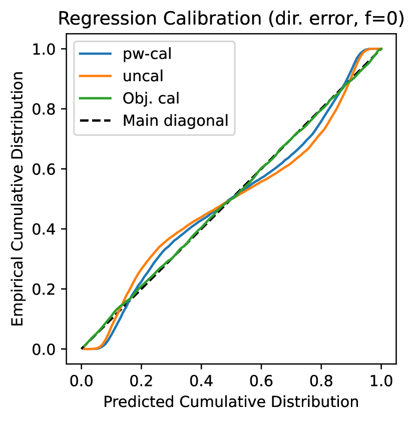
(a)

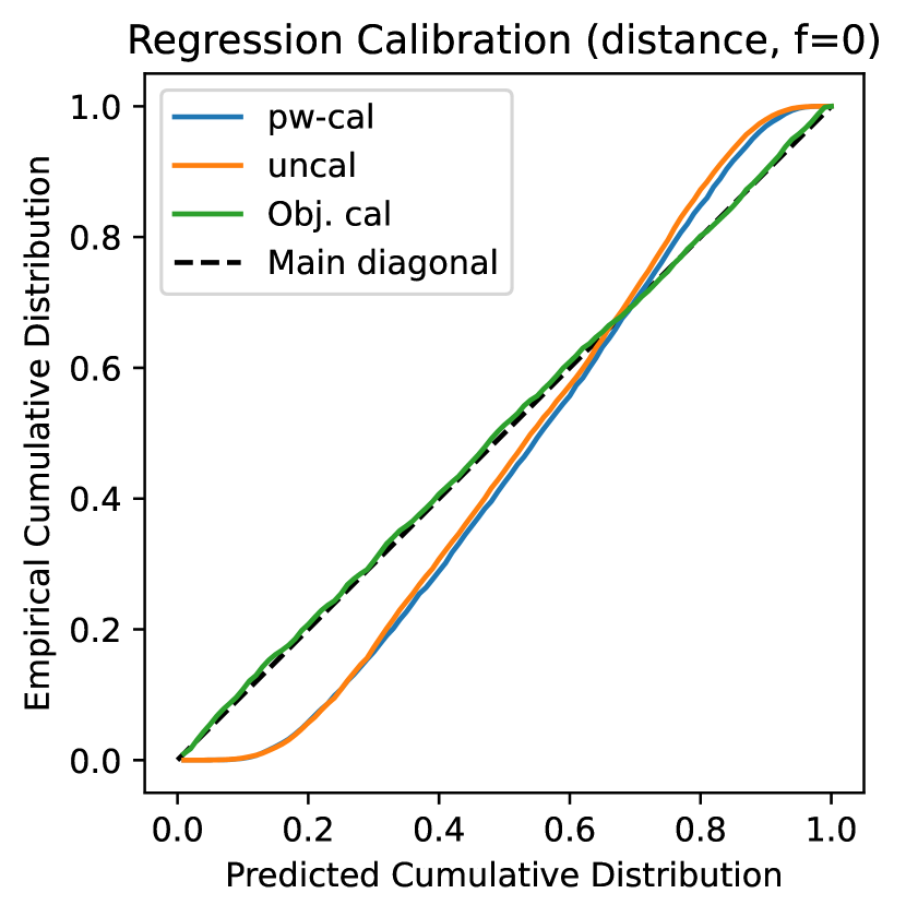
(b)

Figure 2: Regression calibration plot (Kuleshov et al., 2018) for object’s location probabilities: (a) direction error and (b) distance. The Figures have results on uncalibrated (uncal), pixel-wise calibrated (pw-cal), and object-wise calibrated (Obj. cal). The black dashed line shows perfect calibration.

3.2 Probabilistic object presence

A probabilistic object presence $p_{obj}$ is modeled using single probability. In experiments, approximately 99 percent of the probabilistic area under the location is considered. To correct the probability prediction, it is divided by 5, the median pedestrian size. Each detected object is matched with ground truth similar to the previous subsection 3.1. The only difference is that also unmatched detection is used for checking calibration, as all detections are needed for uncertainty analyses.

Again, we ran the same experiments three times, first using uncalibrated semantic segmentation as input for generating detections (uncal) and second using pixel-wise calibrated semantic segmentation for finding detections (pw-cal). Finally, in the object-wise manner (Obj. cal), the resulting probabilistic object presence is calibrated in addition. The calibration is done on the validation dataset (3477 instances) using Beta Calibration. Results are shown on 13810 test instances.

Figure 3 displays that the predictions are overestimating the probability of pedestrians’ presence. After calibration, these effects are alleviated. This is also indicated by ECE scores: 0.184, 0.110, and 0.018.

Based on the histograms below the reliability diagrams, most of the predictions have very high probabilities. The object-wise calibration moves many instances towards lower probability; thus, the histogram is more evenly distributed.

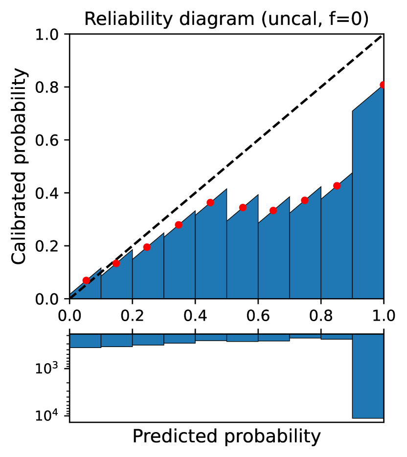
(a)

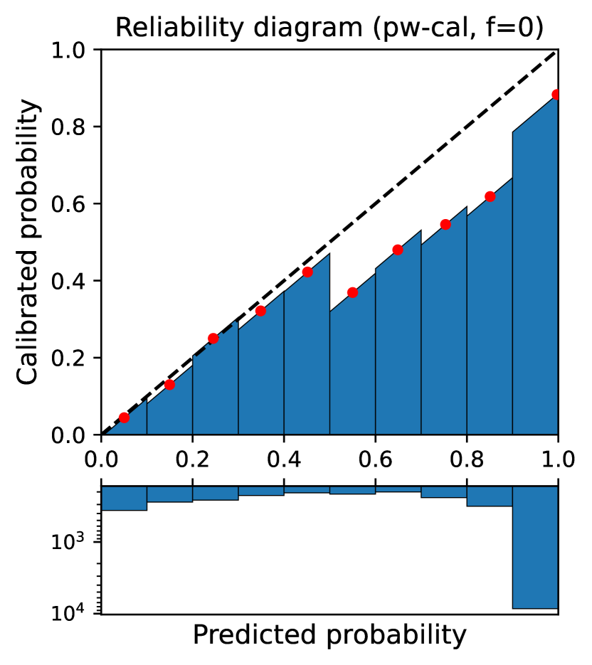
(b)

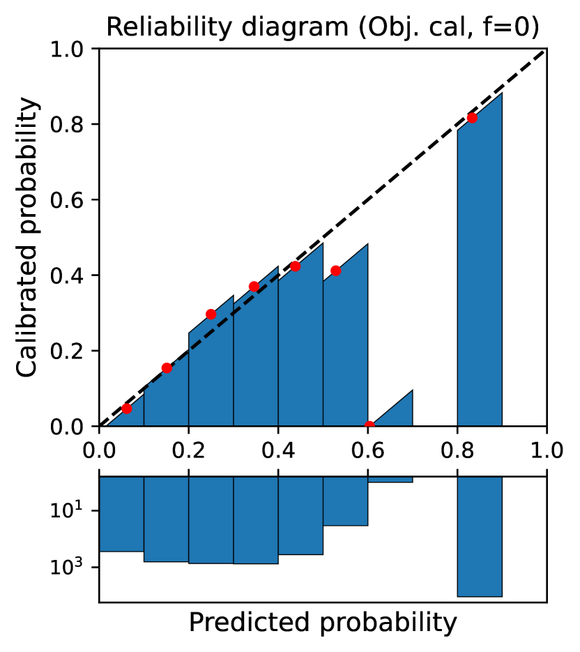
(c)

Figure 3: Reliability diagrams of object’s presence probabilities: (a) uncalibrated, (b) pixel-wise calibrated, and (c) object-wise calibrated. Histograms below the reliability diagrams show how many elements fall into each bin of the reliability diagram. The y-axis for histograms is log-scaled for better comparison. Instances are divided into 10 bins.

3.3 Probabilistic trajectories of objects

Probabilistic trajectories of objects are modeled as a future location $p_{loc}^{f=4}$ and presence of objects $p_{obj}^{f=4}$. These are generated in similar fashion as in two previous subsections 3.1 and 3.2. Based on Figures (Figures 6 and 7 in Appendix A.1), these are acting in a similar manner as for time step 0, $f=0$, so it is possible to conclude that the model is able to predict future time steps ($f=0$) as well-calibrated as current time steps. Furthermore, indicating that the model is able to predict future trajectories quite well for the pedestrian class.

3.4 Probability estimation of undetected-object-ahead by areas

The probability $p_{area}$ is found in a similar way as in subsection 3.2. First, we selected the area 10 meters times 20 meters in front of the vehicle. Then probability of object presence is found and it is checked whether there is any annotated object in the area or not.

In Figure 4 for uncalibrated data, the model underestimates the probability in most of the bins, which means that chance of missing an object is higher than expected. For pixel-wise calibrated cases, it tends to be another way, resulting in worse ECE. The object-wise calibration has the best calibration. The ECE scores are the following: 0.011, 0.069, and 0.003. The equal-size binning is used as most of the probabilities in front of the vehicle are really small. There are only a few (30) undetected objects in the selected area of 4096 test frames; to have more concrete results, more data should be collected and analysed.

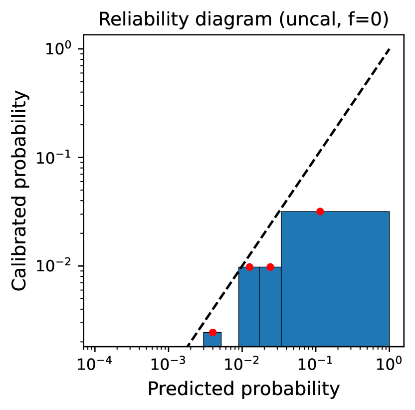
(a)

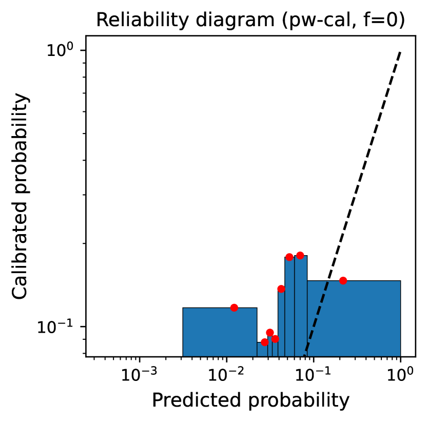
(b)

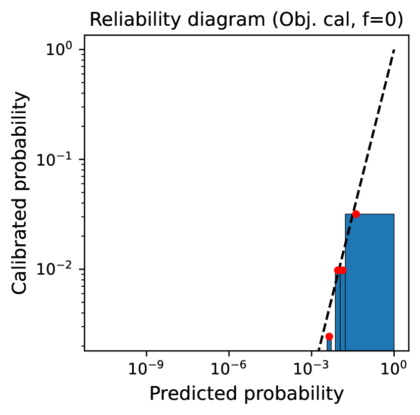
(c)

Figure 4: Reliability diagrams of undetected-object-ahead probabilities: (a) uncalibrated, (b) pixel-wise calibrated, and (c) object-wise calibrated. Data in reliability diagrams are divided equally in bins (equal-size binning), and the axes are log-scaled for better visibility. Instances are divided into 10 bins.

3.5 Calibration of Semantic Segmentation

Semantic segmentation predicted by FIERY contains 200x200 pixels, each for 0.5x0.5 meters area. So in total, 50 meters on each side around the ego-vehicle. The calibration of the semantic segmentation is done in a pixel-wise manner. For calibration Isotonic Regression (Zadrozny and Elkan, 2002) is used. The calibration is done on 20 percent of validation frames (40 million pixels), and the model is evaluated on the remaining 80 percent of test frames (186 million pixels). Uncalibrated ECE (0.00035) is worse than pixel-wise calibrated ECE (0.000013). Further, calibration improves NLL (0.00347) over NLL (0.00322).

In Figure 5, the uncalibrated semantic segmentation is over-estimating the probabilities for segmentation pixels. After calibration, these effects are alleviated as the bins are much closer to the diagonal. Finally, subplot (c) with equal-size binning displays the calibration of low probability pixels, as there were many low probability pixels. The reliability diagram indicates that low probability predictions are also well-calibrated.

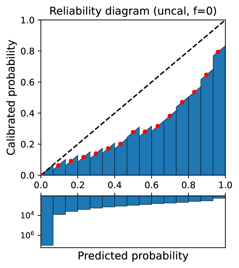
(a)

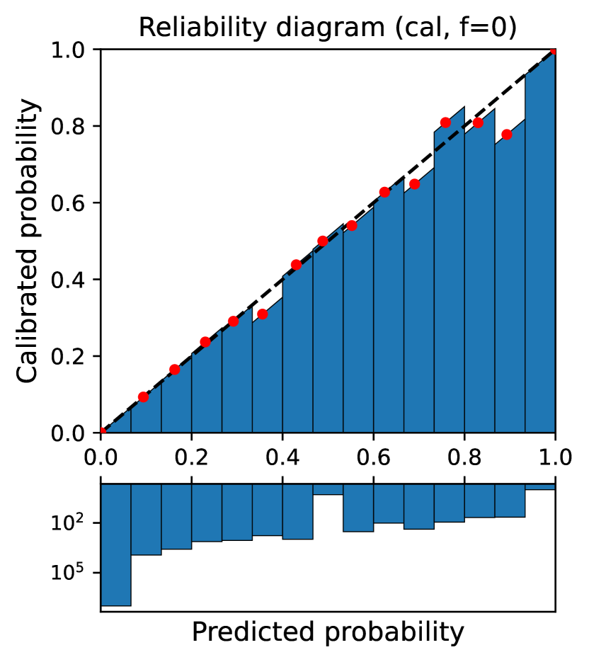
(b)

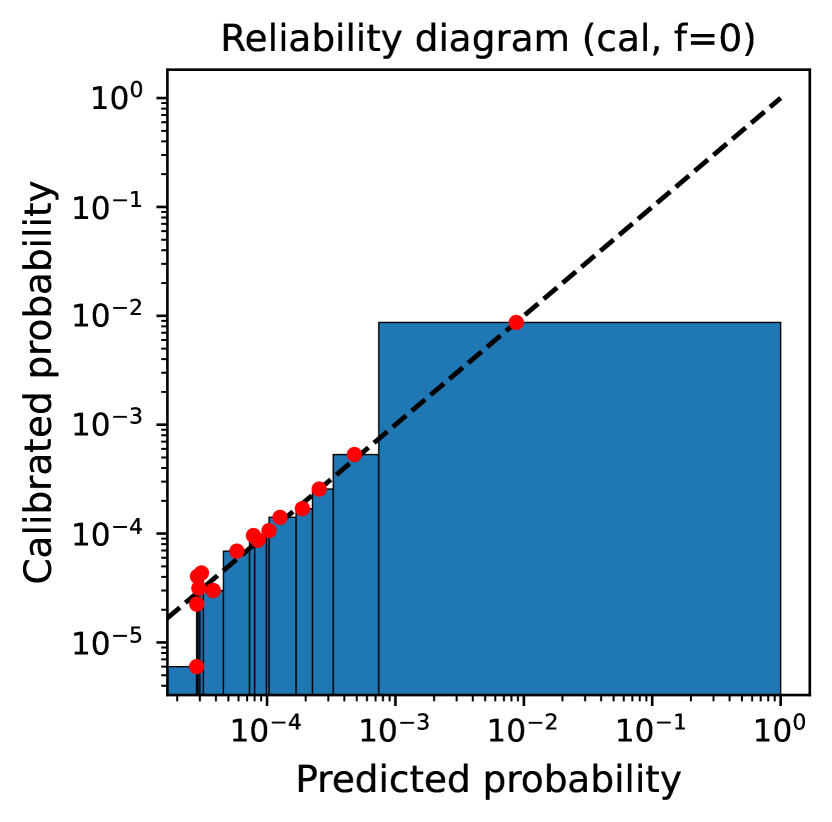
(c)

Figure 5: Reliability diagrams of pixel-wise semantic segmentation calibration: (a) uncalibrated, (b) pixel-wise calibrated with equal-width binning, and (c) pixel-wise calibrated with equal-size binning. Instances are divided into 15 bins.

4 Discussion

Based on the results of experiments, we are able to calibrate all different uncertainties quite well. Pixel-wise calibration is able to calibrate semantic segmentation, but does not convert well to object-wise uncertainties. Thus, object-wise uncertainties are calibrated separately. FIERY model is able to predict pedestrians well, however, it is not certain enough as predictions for pedestrians are not concrete and are drawn out over larger area. Thus, predictions of undetected-object-ahead have too high probabilities for safe driving. This could be alleviated by larger number of examples and more precise annotations. Our work includes couple of limitations. Firstly, we experimented on binary segmentation, in real world, segmentation should involve all necessary classes. Secondly, our work does not address the computational efficiency of uncertainty aspect.

5 Conclusion

In conclusion, a novel way to model probabilities of detections was introduced. These are probabilistic object location, shape, presence, trajectory, and probabilistic undetected-object-ahead by areas. In the experiments, we showed how to model these probabilities from semantic segmentation on pedestrian class. As a result, these probabilities were not calibrated; using object-wise calibration was able to calibrate these probabilities. Using only pixel-wise calibration was not able to capture enough information about object-wise relations of these probabilities. However, it still was able to get a more calibrated object presence. Future work includes out-of-distribution and data set shifts.

6 Acknowledgments

This work was supported by the Estonian Research Council grant PRG1604, by Bolt Technology OÜ grant LLTAT21278, and by the European Social Fund via IT Academy programme.

Appendix A Appendix

A.1 Additional Figures from Experiments

This Section has additional Figures not covered in Experiments Section.

Figures 6 and 7 display results on future timestep ($f=4$). For uncalibrated and pixel-wise calibrated object presence and location these are not well-calibrated. However, object-wise calibration is able to well-calibrate the probabilistic object presence and location.

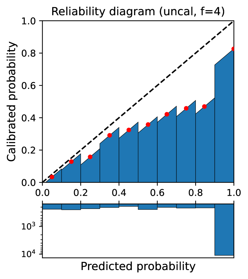
(a)

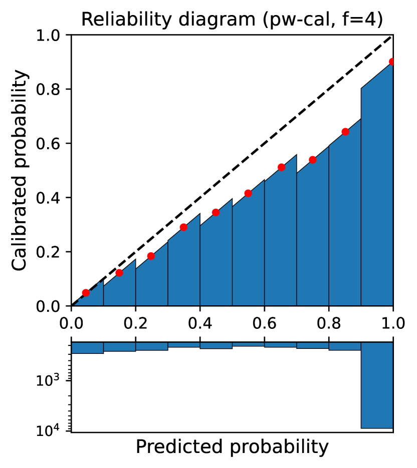
(b)

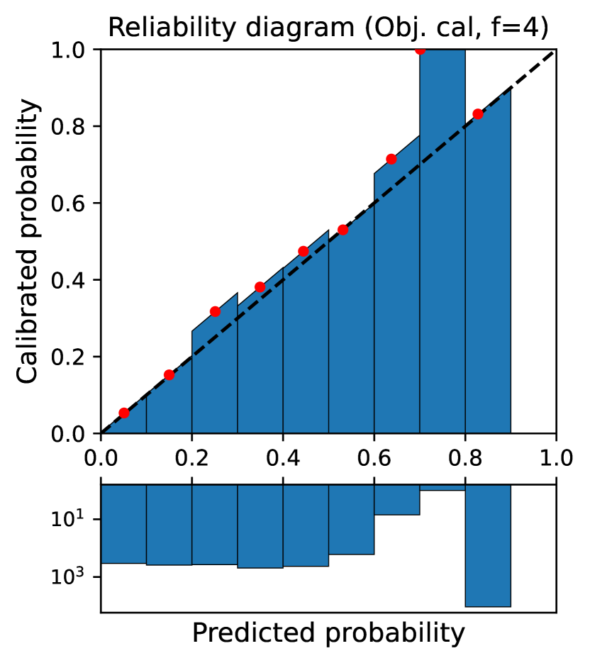
(c)

Figure 6: Reliability diagrams of object’s presence probabilities: (a) uncalibrated, (b) pixel-wise calibrated, and (c) object-wise calibrated. Histograms below the reliability diagrams show how many elements fall into each bin of the reliability diagram. The y-axis for histograms is log-scaled for better comparison. $f=4$ stands for fourth future time step (4 seconds in future). Instances are divided into 10 bins.

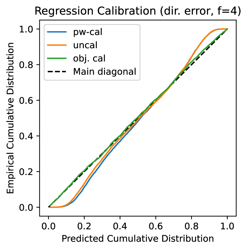
(a)

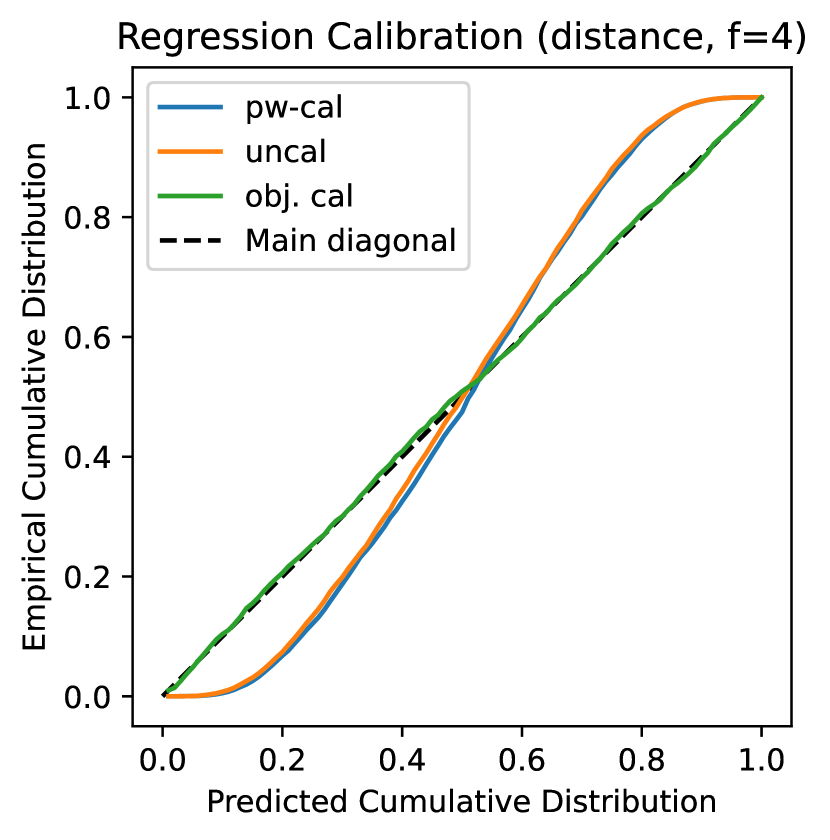
(b)

Figure 7: Regression calibration plot [Kuleshov et al., 2018] for object’s location probabilities: (a) direction error and (b) distance. The Figures have results on uncalibrated (uncal), pixel-wise calibrated (pw-cal), and object-wise calibrated (obj. cal). The black dashed line shows perfect calibration. $f=4$ stands for fourth future time step (4 seconds in future).

References

- Allikivi and Kull (2019) Mari-Liis Allikivi and Meelis Kull. Non-parametric bayesian isotonic calibration: Fighting over-confidence in binary classification. In Joint European Conference on Machine Learning and Knowledge Discovery in Databases, pages 103–120. Springer, 2019.
- Amodei et al. (2016) Dario Amodei, Chris Olah, Jacob Steinhardt, Paul Christiano, John Schulman, and Dan Mané. Concrete problems in ai safety. arXiv preprint arXiv:1606.06565, 2016.
- Caesar et al. (2019) Holger Caesar, Varun Bankiti, Alex H. Lang, Sourabh Vora, Venice Erin Liong, Qiang Xu, Anush Krishnan, Yu Pan, Giancarlo Baldan, and Oscar Beijbom. nuscenes: A multimodal dataset for autonomous driving. arXiv preprint arXiv:1903.11027, 2019.
- Choi et al. (2019) Jiwoong Choi, Dayoung Chun, Hyun Kim, and Hyuk-Jae Lee. Gaussian yolov3: An accurate and fast object detector using localization uncertainty for autonomous driving. In Proceedings of the IEEE/CVF International Conference on Computer Vision, pages 502–511, 2019.
- Choset et al. (2005) Howie Choset, Kevin M Lynch, Seth Hutchinson, George A Kantor, and Wolfram Burgard. Principles of robot motion: theory, algorithms, and implementations. MIT press, 2005.
- Claussmann et al. (2019) Laurene Claussmann, Marc Revilloud, Dominique Gruyer, and Sébastien Glaser. A review of motion planning for highway autonomous driving. IEEE Transactions on Intelligent Transportation Systems, 21(5):1826–1848, 2019.
- Gonzalez and Stentz (2007) Juan Pablo Gonzalez and Anthony Stentz. Planning with uncertainty in position using high-resolution maps. In Proceedings 2007 IEEE International Conference on Robotics and Automation, pages 1015–1022. IEEE, 2007.
- Gruyer et al. (2017) Dominique Gruyer, Valentin Magnier, Karima Hamdi, Laurène Claussmann, Olivier Orfila, and Andry Rakotonirainy. Perception, information processing and modeling: Critical stages for autonomous driving applications. Annual Reviews in Control, 44:323–341, 2017.
- Hu et al. (2021) Anthony Hu, Zak Murez, Nikhil Mohan, Sofía Dudas, Jeffrey Hawke, Vijay Badrinarayanan, Roberto Cipolla, and Alex Kendall. Fiery: Future instance prediction in bird’s-eye view from surround monocular cameras. In Proceedings of the IEEE/CVF International Conference on Computer Vision, pages 15273–15282, 2021.
- Kängsepp et al. (2022) Markus Kängsepp, Kaspar Valk, and Meelis Kull. On the usefulness of the fit-on-the-test view on evaluating calibration of classifiers. arXiv preprint arXiv:2203.08958, 2022.
- Koopman (2022) Philip Koopman. How Safe Is Safe Enough?: Measuring and Predicting Autonomous Vehicle Safety. Independently published, 2022.
- Kuleshov et al. (2018) Volodymyr Kuleshov, Nathan Fenner, and Stefano Ermon. Accurate uncertainties for deep learning using calibrated regression. In International conference on machine learning, pages 2796–2804. PMLR, 2018.
- Kull et al. (2017) Meelis Kull, Telmo Silva Filho, and Peter Flach. Beta calibration: a well-founded and easily implemented improvement on logistic calibration for binary classifiers. In Artificial Intelligence and Statistics, pages 623–631. PMLR, 2017.
- Kuwata et al. (2009) Yoshiaki Kuwata, Justin Teo, Gaston Fiore, Sertac Karaman, Emilio Frazzoli, and Jonathan P How. Real-time motion planning with applications to autonomous urban driving. IEEE Transactions on control systems technology, 17(5):1105–1118, 2009.
- Mouhagir et al. (2016) Hafida Mouhagir, Reine Talj, Véronique Cherfaoui, François Aioun, and Franck Guillemard. Integrating safety distances with trajectory planning by modifying the occupancy grid for autonomous vehicle navigation. In 2016 IEEE 19th international conference on intelligent transportation systems (ITSC), pages 1114–1119. IEEE, 2016.
- Naeini et al. (2015) Mahdi Pakdaman Naeini, Gregory Cooper, and Milos Hauskrecht. Obtaining well calibrated probabilities using bayesian binning. In Twenty-Ninth AAAI Conference on Artificial Intelligence, 2015.
- Niculescu-Mizil and Caruana (2005) Alexandru Niculescu-Mizil and Rich Caruana. Predicting good probabilities with supervised learning. In Proceedings of the 22nd international conference on Machine learning, pages 625–632, 2005.
- Ok et al. (2013) Kyel Ok, Sameer Ansari, Billy Gallagher, William Sica, Frank Dellaert, and Mike Stilman. Path planning with uncertainty: Voronoi uncertainty fields. In 2013 IEEE International Conference on Robotics and Automation, pages 4596–4601. IEEE, 2013.
- Paden et al. (2016) Brian Paden, Michal Čáp, Sze Zheng Yong, Dmitry Yershov, and Emilio Frazzoli. A survey of motion planning and control techniques for self-driving urban vehicles. IEEE Transactions on intelligent vehicles, 1(1):33–55, 2016.
- Redmon and Farhadi (2018) Joseph Redmon and Ali Farhadi. Yolov3: An incremental improvement. arXiv preprint arXiv:1804.02767, 2018.
- Veres et al. (2010) Sandor Veres, Levente Molnar, Nick Lincoln, and Colin Morice. Autonomous vehicle control systems - a review of decision making. IMechE Journal of Systems and Control, 225, 05 2010. doi: 10.1177/2041304110394727.
- Yang et al. (2019) Bo Yang, Jianan Wang, Ronald Clark, Qingyong Hu, Sen Wang, Andrew Markham, and Niki Trigoni. Learning object bounding boxes for 3d instance segmentation on point clouds. Advances in neural information processing systems, 32, 2019.
- Zadrozny and Elkan (2002) Bianca Zadrozny and Charles Elkan. Transforming classifier scores into accurate multiclass probability estimates. In Proceedings of the eighth ACM SIGKDD international conference on Knowledge discovery and data mining, pages 694–699, 2002.