Resolution enhancement of one-dimensional molecular wavefunctions in plane-wave basis via quantum machine learning

Abstract

Super-resolution is a machine-learning technique in image processing which generates high-resolution images from low-resolution images. Inspired by this approach, we perform a numerical experiment of quantum machine learning, which takes low-resolution (low plane-wave energy cutoff) one-particle molecular wavefunctions in plane-wave basis as input and generates high-resolution (high plane-wave energy cutoff) wavefunctions in fictitious one-dimensional systems, and study the performance of different learning models. We show that the trained models can generate wavefunctions having higher fidelity values with respect to the ground-truth wavefunctions than a simple linear interpolation, and the results can be improved both qualitatively and quantitatively by including data-dependent information in the ansatz. On the other hand, the accuracy of the current approach deteriorates for wavefunctions calculated in electronic configurations not included in the training dataset. We also discuss the generalization of this approach to many-body electron wavefunctions.

I introduction

Quantum machine learning (QML) is considered to be one of the potential promising applications of near-term and future quantum computing [1, 2]. Hybrid classical-quantum QML algorithms with a parameterized quantum circuit (PQC) [3] are extensively studied as a practical application of noisy intermediate-scale quantum (NISQ) devices, and fully quantum approaches, such as quantum support vector machines [4], have also been proposed.

Although significant progress has been made in this field, it is still unclear if QML applied on classical input data can offer quantum advantage, except for a few special cases [5, 6, 7, 8, 9]. A new direction in QML is to use quantum states directly as input data [10, 11]. This approach is most straightforwardly applicable to problems in physical science if quantum states of physical objects are encoded as input data into QML. Many-body wavefunctions are a representative input for classification of topological or magnetic phases [12, 13, 14, 15], and molecular electronic wavefunctions are also used [16, 17]. While encoding of the classical input data into quantum states is a highly nontrivial problem in QML [18, 19], no such issue arises when learning directly on quantum data. In this case, the performance of a QML model is solely determined by the structure of the ansatz, i.e., the arrangement of the parameterized unitaries, to be employed.

In this work, we consider a different type of QML experiment with quantum input using one-particle molecular electronic wavefunctions, inspired by the super-resolution technique developed in the field of (classical) machine learning. Through this experiment, we study how we can improve QML models with quantum input. As a possible improvement for QML model, we explore the possibility of adding classical information to quantum input data in a scheme similar to the data re-uploading [20, 21, 22]. The single-image super-resolution is an image processing technique which generates a high-resolution (HR) image from a low-resolution (LR) image [23, 24]. Existing works on super-resolution are based on several deep learning approaches, such as deep convolutional networks [25] and generative adversarial networks [26]. A potential future application of this work is to generate approximate electron wavefunctions in high-throughput quantum chemistry calculations with low computational cost.

We consider molecular one-particle wavefunctions expressed in plane waves. The plane-wave basis is a flexible basis widely used in the electronic structure calculations of solid-state systems [27], and several quantum algorithms based on plane-wave expansion of the wavefunctions have recently been proposed for fault-tolerant quantum computers, both in the second and first quantization formalisms [28, 29, 30, 31, 32, 33]. In this work, “low-resolution” wavefunctions are expressed with a small number of plane waves (low plane-wave energy cutoff), and by using them as input of QML we aim to construct “high-resolution” wavefunctions which are expressed with a larger number of plane waves. As a benchmark test of this approach, we consider fictitious molecular systems in one spatial dimension [34].

The state of an electronic system with a fixed number of particles can be encoded into a quantum register through either the first or second quantization approaches. The first option may use significantly fewer qubits, especially when the number of particles is small, while the second option uses as many qubits as the number of basis functions. Because our one-particle wavefunctions are expanded into up to 31 plane-waves, we opt for the first quantization encoding. The price we have to pay for this dense encoding in first quantization is that the resulting quantum states are highly entangled. In our experiments, we use exact amplitude encoding for the LR/HR wavefunctions and use rather deep parameterized circuits with a statevector-based quantum simulator. Simplification of the ansatzes and consideration of various runtime errors, which would be required for this work to be practically applicable in the NISQ era, are left for future research. We also discuss a generalization of this approach to many-body wavefunctions.

II method

II.1 Molecular orbitals in plane-wave basis

We consider fictitious one-dimensional molecular systems interacting via exponential Coulomb-mimicking functions proposed in Ref. [34], although the current approach can be generalized to treat general three-dimensional systems. We impose a periodic boundary condition with periodicity $L$ and expand the one-particle wavefunctions (molecular orbitals) $\psi_{\mu\sigma}(x)$ with $N_{\textrm{pw}}$ plane-wave basis functions $\chi_{k_{j}}(x)$ as

$$\psi_{\mu\sigma}(x)=\sum_{k_{j}}C_{k_{j}\mu\sigma}\chi_{k_{j}}(x),$$ (1)

where $\mu$ and $\sigma$ are spatial orbital and spin indices, respectively, and

$$\chi_{k_{j}}(x)=\frac{1}{\sqrt{L}}e^{ik_{j}x},$$ (2)

$$k_{j}=\frac{2\pi}{L}j\quad j=0,\pm 1,\pm 2,\dots,\pm\frac{N_{\textrm{pw}}-1}{2}.$$ (3)

We consider odd $N_{\textrm{pw}}$. The expansion coefficients $C_{k_{j}\mu\sigma}$ are determined by solving the following Hartree-Fock equation self-consistently

$$\sum_{k_{j^{\prime}}}h^{\textrm{HF}\sigma}_{jj^{\prime}}C_{k_{j^{\prime}}\mu\sigma}=\varepsilon_{\mu\sigma}C_{k_{j}\mu\sigma},$$ (4)

where $h^{\textrm{HF}}$ is the Hartree-Fock one-particle Hamiltonian matrix and $\varepsilon_{\mu\sigma}$ are Hartree-Fock eigenenergies. The details of the calculations are given in Appendix A.

II.2 Quantum circuit for resolution enhancement

Figure 1: Quantum circuit to calculate the fidelity between the $i$-th true HR wavefunction and the predicted wavefunction generated from the corresponding LR data.

Figure 2: The initialization operation $U_{\textrm{init}}$ (first CNOT gate) and the shift operation $U^{(i)}_{\textrm{shift}}$ ($e^{ik_{j}d^{(i)}_{\textrm{CM}}}$) in Fig. 1 for $n_{\textrm{LR}}=3$. Here $k_{j}$ are plane-wave wavevectors, and $d^{(i)}_{\textrm{CM}}$ is the center of mass for the $i$-th data.

We encode the LR molecular wavefunction coefficients $C^{\textrm{LR}}_{k_{j}\mu\sigma}$ for $N^{\textrm{LR}}_{\textrm{pw}}$ plane waves in a quantum circuit as the amplitudes of $n_{\textrm{LR}}=\lceil\log_{2}N_{\textrm{pw}}^{\textrm{LR}}\rceil$ qubit states, and generate the HR wavefunction coefficients $C^{\textrm{HR}}_{k_{j}\mu\sigma}$ for $N^{\textrm{HR}}_{\textrm{pw}}(>N^{\textrm{LR}}_{\textrm{pw}})$ plane waves with $n_{\textrm{HR}}=\lceil\log_{2}N_{\textrm{pw}}^{\textrm{HR}}\rceil$ qubits, using parametrized quantum circuits whose parameters are determined by minimizing some cost function. We consider the case $n_{\textrm{HR}}=n_{\textrm{LR}}+1$, although more general resolution enhancement ($n_{\textrm{HR}}=n_{\textrm{LR}}+m,m\in\mathbb{N}$) is also possible. We consider the case where the LR wavefunctions are underconverged. Under this condition, the HR wavefunctions cannot be obtained by a simple interpolation of the corresponding LR wavefunctions in real space, but have to be obtained by the extrapolation of the LR wavefunction coefficients $C_{k_{j}\mu\sigma}$ in the Fourier (wavevector) space. We prepare LR/HR wavefunction pairs $\{\psi_{\text{LR/HR}}^{(i)}\}_{i=1}^{N_{\text{data}}}$ as datasets and try to find $U(\bm{\theta},\bm{D}^{(i)})$ which can generate approximate HR wavefunctions $|\tilde{\psi}_{\text{HR}}^{(i)}\rangle$ from LR wavefunctions as $|\tilde{\psi}_{\text{HR}}^{(i)}\rangle=U(\bm{\theta},\bm{D}^{(i)})|0\rangle\otimes|\psi^{(i)}_{\text{LR}}\rangle$ by optimizing parameters $\theta$. Here $i$ is the sample index. The ansatz $U(\bm{\theta},\mathbf{D}^{(i)})$ may also depend on the data-dependent parameters $\mathbf{D}^{(i)}$ for the sample $i$. The state $|\psi^{(i)}_{\textrm{LR}}\rangle$ is the $i$-th LR wavefunction expressed using $n_{\textrm{LR}}$ qubits. Unitary operations guarantee that LR plane-wave basis wavefunctions are mapped to orthonormal HR wavefunctions. The parameters $\bm{\theta}$ are optimized by maximizing the fidelity between the predicted and the true HR orbitals, or equivalently by minimizing the cost function

$$\mathcal{L}=-\frac{1}{N_{\textrm{data}}}\sum_{i=1}^{N_{\textrm{data}}}|\langle\psi^{(i)}_{\textrm{HR}}|\tilde{\psi}^{(i)}_{\textrm{HR}}\rangle|^{2}.$$ (5)

Figure 1 shows the quantum circuit used to compute the fidelity between $|\psi^{(i)}_{\textrm{HR}}\rangle$ and $|\tilde{\psi}^{(i)}_{\textrm{HR}}\rangle$. Here $V_{\textrm{LR}}^{(i)}$ and $V_{\textrm{HR}}^{(i)}$ are unitary operations to encode $C^{\textrm{LR}(i)}_{k_{j}\mu\sigma}$ and $C^{\textrm{HR}(i)}_{k_{j}\mu\sigma}$, respectively. We encode the LR wavefunctions as

$$|\psi^{(i)}_{\textrm{LR}}\rangle=V_{\textrm{LR}}^{(i)}|0\rangle^{\otimes n_{\textrm{LR}}}=\sum_{j=-\frac{N^{\textrm{LR}}_{\textrm{pw}}-1}{2}}^{+\frac{N^{\textrm{LR}}_{\textrm{pw}}-1}{2}}C^{\textrm{LR}(i)}_{k_{j}\mu\sigma}|k_{j}\rangle,$$ (6)

where $|k_{j}\rangle$ are expressed by following the convention in the Fast Fourier Transform [36]

$$|k_{j}\rangle=\left\{\begin{array}[]{ll}|j\rangle&(j\geq 0)\\ |j+2^{n_{\textrm{LR}}}\rangle&(j<0)\end{array}\right.$$ (7)

with $|j\rangle$ the binary representation of $j$. The HR wavefunctions are similarly embedded in the HR space with $n_{\textrm{HR}}=n_{\text{LR}}+1$ qubits with $V_{\textrm{HR}}^{(i)}$. The two unitaries $U_{\textrm{init}}$ and $U^{(i)}_{\textrm{shift}}$ in Fig. 1 are the initialization and shifting operations, respectively, which are described below. The fidelity is obtained as the probability of observing $|0\rangle^{\otimes n_{\textrm{HR}}}$ in the measurements in Fig. 1.

Figure 2 shows the initialization part of Fig. 1. The first CNOT reorders the coefficients $C^{\textrm{LR}(i)}_{k_{j}\mu\sigma}$ in the $2^{n_{\textrm{LR}}+1}$-dimensional space, and the second operation multiplies a phase factor $e^{ik_{j}d^{(i)}_{\textrm{CM}}}$ to each of the plane-wave basis, which corresponds to setting the origin to $d_{\textrm{CM}}^{(i)}$, the center of mass of sample $i$.

II.3 Dataset and ansatz

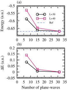
Figure 3: (a) The calculated energy of a hydrogen atom for $L=30$ a.u. (circles) and $L=40$ a.u. (squares) with $N_{\textrm{pw}}=7,15,31$. The result of a real space grid approach in Ref. [34] ($E_{\textrm{ref}}=-0.670$) is also shown as a dashed line for comparison. (b) The energy difference defined as $|E-E_{\textrm{ref}}|$.

As a benchmark test of the approach, we consider the wavefunctions of the systems consisting of hydrogen atoms, H_x, similar to those used in Ref. [35]. We consider only symmetric molecules and place them so that their centers are at $x=0$. With this choice, the wavefunction coefficients $C_{k_{j}\mu\sigma}$ can be chosen to be real, and the shifting operation $U^{(i)}_{\textrm{shift}}$ in Fig. 1 is not required. We use 52 Hartree-Fock occupied wavefunctions for training, and the trained model is applied to the validation dataset, which includes molecules not included in the training dataset and uses a finer bond length grid. The details of the training and validation datasets are described in Appendix B.

Two cases are considered in our experiments: (i) LR (HR) wavefunctions are constructed with $N_{\textrm{pw}}=7\ (15)$ plane waves at $L=30$ a.u.; (ii) LR (HR) wavefunctions are constructed with $N_{\textrm{pw}}=15\ (31)$ plane waves at $L=40$ a.u.. The number of qubits used in our experiments is four and five for cases (i) and (ii), respectively. The total energies of a hydrogen atom calculated with these parameters are shown in Figs. 3 (a, b). In case (i) ($N_{\textrm{pw}}:7\to 15$) the Fourier wavevector grid of the LR wavefunctions is very coarse, making the LR wavefunctions very crude approximations, while in case (ii) ($N_{\textrm{pw}}:15\to 31$) the grid is finer and the LR wavefunctions are closer to the exact wavefunctions. With $N_{\textrm{pw}}=31$, the calculated energy values are within 0.01 a.u. of the reference energy obtained from a real space grid approach in Ref. [34] for both $L=30$ and $L=40$.

Two classes of ansatzes are employed as the unitary $U(\bm{\theta},\mathbf{D}^{(i)})$: the first (ansatz 1) is a general ansatz for real amplitudes and is independent of the input sample,

$$U(\bm{\theta})=\prod_{l=1}^{N_{\textrm{layer}}}\Bigl{[}\Bigl{(}\prod_{i_{q}=1}^{n_{q}}R^{i_{q}}_{y}(\theta_{i_{q},l})\Bigr{)}U_{\textrm{Ent}}\Bigr{]}\prod_{i_{q}=1}^{n_{q}}R^{i_{q}}_{y}(\theta_{i_{q},0}),$$ (8)

where $N_{\textrm{layer}}$ and $n_{q}$ are the number of layers and qubits, respectively, and $U_{\textrm{Ent}}$ is an entangling operator consisting of $n_{q}-1$ CNOT gates connecting the $i$-th and $(i+1)$-th qubits. The total number of parameters in this class of ansatzes is $n_{q}(N_{\textrm{layer}}+1)$. See Fig. 4 for a circuit diagram.

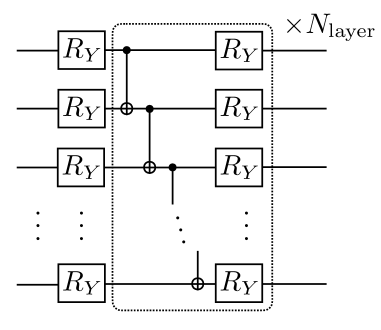
Figure 4: Circuit diagram of ansatz 1.

The second class (ansatz 2) consists of sample-dependent ansatzes inspired by the Fourier-transformed variational Hamiltonian ansatz [37]

$$U(\bm{\theta},\mathbf{D}^{(i)})=\prod_{l=1}^{N_{\textrm{layer}}}U_{\textrm{HEA}}(\bm{\theta}_{l})\textrm{QFT}^{\dagger}e^{-i\theta_{l,0}\mathcal{V}^{(i)}(x)}\textrm{QFT},$$ (9)

where $U_{\textrm{HEA}}$ is a hardware-efficient ansatz

$$U_{\textrm{HEA}}(\bm{\theta}_{l}) = \prod_{\tilde{l}=1}^{\tilde{N}_{\textrm{layer}}}\Bigl{[}\Bigl{(}\prod_{i_{q}=1}^{n_{q}}R^{i_{q}}_{z}(\theta_{l,i_{q},\tilde{l},z})R^{i_{q}}_{x}(\theta_{l,i_{q},\tilde{l},x})\Bigr{)}U_{\textrm{Ent}}\Bigr{]}$$ (10)

$$\times\prod_{i_{q}=1}^{n_{q}}R^{i_{q}}_{z}(\theta_{l,i_{q},0,z})R^{i_{q}}_{x}(\theta_{l,i_{q},0,x}),$$

with $\tilde{N}_{\textrm{layer}}$ the number of sublayers. The corresponding circuit diagram is shown in Fig. 5. The first QFT in Eq. (9) performs the Quantum Fourier Transform and transforms the input LR wavefunction from the Fourier space to real space, $|k_{j}\rangle\to|x_{j}\rangle$. The following operator adds phase factors to the states as $|x_{j}\rangle\to e^{-i\theta_{l,0}\mathcal{V}^{(i)}(x_{j})}|x_{j}\rangle$, where $\mathcal{V}^{(i)}(x)$ is a sample-dependent effective one-particle potential. While $\mathcal{V}^{(i)}(x)$ can be any function of the electron position $x$ in principle, we use the electron-nuclei Coulomb potential $v_{\textrm{en}}(x)$ in Eq. (21), which depends only on the numbers and positions of the atoms in each sample, as the simplest choice. The wavefunction is transformed back to the Fourier space with the next QFT^† before the last operation $U_{\textrm{HEA}}(\bm{\theta}_{l})$, which accounts for the kinetic part of the Hamiltonian and also other effects not included in $e^{-i\theta_{l,0}\mathcal{V}^{(i)}(x)}$.

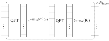
(a) full ansatz

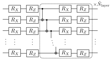
(b) HEA part

Figure 5: Circuit diagram of ansatz 2.

We choose the number of layers $N_{\textrm{layer}}=32$ for ansatz 1 (Eq. (8)). We use this large number of layers to provide this model with sufficient flexibility. We observe that increasing the number of layers up to $N_{\textrm{layer}}=64$ does not improve the results significantly. For ansatz 2 (Eq. (9)), $N_{\textrm{layer}}=3,\tilde{N}_{\textrm{layer}}=8$ are used. The number of variational parameters in ansatz 1 (ansatz 2) are 132 (219) and 165 (273) for case (i) and case (ii), respectively. Because of the data-dependent potential term, ansatz 2 is more easily trapped in local minima than ansatz 1. We find that starting with $\bm{\theta}=0$ in ansatz 2 generally shows a good convergence. We use the PennyLane library [38] and minimize the cost function (Eq. (5)) using the Adam optimizer.

II.4 Extension to many-body wavefunctions

Figure 6: Quantum circuit to generate a HR two-electron wavefunction from the $i$-th LR wavefunction $\Psi^{(i)}_{2,\textrm{LR}}$ (represented by the first four qubits of the circuit) for $n_{\textrm{LR}}=2$.

In this section we consider whether we can apply the model trained with one-particle wavefunctions directly to enhance the resolution of many-body wavefunctions. Neglecting spin degrees of freedom for simplicity, in first quantization, the $N_{\textrm{el}}$-electron wavefunctions can be written with $N_{\textrm{el}}\lceil\log_{2}N_{\textrm{pw}}\rceil$ qubits as [31]

$$|\Psi_{N_{\textrm{el}}}\rangle=\sum_{\{k_{j}\}}C_{k_{0}k_{1}\dots k_{N_{\textrm{el}}-1}}|k_{0}k_{1}\dots k_{N_{\textrm{el}}-1}\rangle,$$ (11)

where the expansion coefficients are antisymmetric:

$$C_{\dots k_{i}\dots k_{j}\dots}=-C_{\dots k_{j}\dots k_{i}\dots}.$$ (12)

When $U(\bm{\theta},\mathbf{D}^{(i)})$ does not contain orbital-dependent parameters, as in ansatz 1 and ansatz 2 in the previous section, one can generate an approximate antisymmetric HR many-body wavefunction from a LR many-body state expressed with $N_{\textrm{el}}n_{\textrm{LR}}$ qubits and with extra $N_{\textrm{el}}$ qubits, $|\Psi^{\textrm{LR}(i)}_{N_{\textrm{el}}}\rangle\otimes|0\rangle^{\otimes N_{\textrm{el}}}$, by applying $\bar{U}^{(i)}=U(\bm{\theta},\mathbf{D}^{(i)})U_{\textrm{shift}}^{(i)}U_{\textrm{init}}$ to each of the $N_{\textrm{el}}$ registers as

$$|\tilde{\Psi}^{\textrm{HR}(i)}_{N_{\textrm{el}}}\rangle \approx \Bigl{[}\bar{U}^{(i)}\otimes\bar{U}^{(i)}\otimes\cdots\otimes\bar{U}^{(i)}\Bigr{]}$$ (13)

$$U_{\textrm{SWAP}}|\Psi^{\textrm{LR}(i)}_{N_{\textrm{el}}}\rangle\otimes|0\rangle^{\otimes N_{\textrm{el}}}.$$

Here, $U_{\textrm{SWAP}}$ is a unitary operation that reorders states $|k_{0}k_{1}\dots k_{N_{\textrm{el}}-1}\rangle\otimes|0\rangle^{\otimes N_{\textrm{el}}}$ to $|0\,k_{0}0\,k_{1}\dots 0\,k_{N_{\textrm{el}}-1}\rangle$ using SWAP gates. The case for $N_{\textrm{el}}=2$ is shown in Fig. 6. Spin degrees of freedom can be included in Eq. (13) by adding extra $N_{\textrm{el}}$ qubits.

Although this procedure is simple and very easy to implement, there are two potential problems in this generalization. First, since a many-body wavefunction is written as a sum of the product of $N_{\textrm{el}}$ one-particle wavefuntion in first quantization, the fidelity between the predicted and true HR wavefunctions, $|\langle\tilde{\Psi}^{\textrm{HR}}_{N_{\textrm{el}}}|\Psi^{\textrm{HR}}_{N_{\textrm{el}}}\rangle|^{2}$, decreases as $O\bigl{(}(f_{1})^{N_{\textrm{el}}}\bigr{)}$, where $f_{1}$ is a typical fidelity of one-particle wavefunctions obtained with the ansatz used. A scalable generalization of this approach to many-body systems would require some correction operation that entangles qubits in different registers and that still keeps the antisymmetry of the wavefunctions. This point is left for our future research. The second problem is the phase of the predicted wavefunctions; in the current approach based on fidelity maximization, the unitary operation $\bar{U}^{(i)}$ can add orbital-dependent phase factors to the predicted one-particle wavefunctions as

$$\bar{U}^{(i)}\psi^{\textrm{LR}}_{\mu\sigma}\approx e^{i\theta_{\mu}^{(i)}}\psi^{\textrm{HR}}_{\mu\sigma}.$$ (14)

This implies that each term in the predicted wavefunction in Eq. (11) can potentially get a different relative phase, resulting in a low-fidelity state. A simple fix to this problem is to consider a linear combination of orbital pairs,

$$\psi^{(i)}_{\mu_{1}\mu_{2}\sigma}=\frac{1}{\sqrt{2}}\Bigl{[}\psi^{(i)}_{\mu_{1}\sigma}+\psi^{(i)}_{\mu_{2}\sigma}\Bigr{]},$$ (15)

and include $\psi^{(i)}_{\mu_{1}\mu_{2}\sigma}$ in the training dataset, which has an effect of aligning the two phases $e^{i\theta_{\mu_{1}}}$ and $e^{i\theta_{\mu_{2}}}$ in Eq. (14). In addition, the phases of LR and HR wavefunctions in the training dataset must also be consistent. This can be done by preprocessing the training dataset, as described in Appendix B.

III results and discussion

III.1 One-electron case

	case (i)	case (ii)
	$N_{\textrm{pw}}:7\to 15,L=30$	$N_{\textrm{pw}}:15\to 31,L=40$
no ansatz	0.890	0.981
ansatz 1	0.959	0.992
ansatz 2	0.983	0.997
linear interpolation	0.839	0.954

Table 1: Calculated average fidelities of the training dataset.

Table  1 shows the calculated average fidelity values between the ground-truth and predicted HR wavefunctions for the training dataset. In the table we also show the results of the linear interpolation in real space calculated with one ancilla qubit, which is detailed in Appendix C. In case (i) ($N_{\textrm{pw}}:7\to 15$), as the LR wavefunctions are very crude approximations of the HR wavefunctions, without including any ansatz we get a low average fidelity of 0.890. The linear interpolation in real space, shown in the last row in Table 1, performs even poorer. Of the two parameterized models, ansatz 2 gives better results. This may owe to the nonlinearity introduced in the model through the inclusion of sample-dependent information in the ansatz. We further note that this information is inserted into the ansatz repeatedly, which may improve the expressibility of the ansatz in a similar manner to the data reuploading technique used to encode classical information into quantum states [20]. In case (ii) ($N_{\textrm{pw}}:15\to 31$) the LR wavefunctions already have high fidelity values with the HR wavefunctions, but the results are improved also in this case by including the two ansatzes.

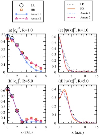
Figure 7: The occupied Hartree-Fock wavefunction of the singlet ground state of H₂ at bond length $R=1.0$ a.u. (a, c) and $R=5.0$ a.u. (b, d) in Fourier space (a, b) and in real space (c, d) at $L=30$ a.u. for $N_{\textrm{pw}}:7\to 15$ resolution enhancement. The hydrogen atoms are located at $x=\pm\frac{R}{2}$. Only $k\geq 0$ and $0\leq x\leq\frac{L}{2}$ regions are shown.

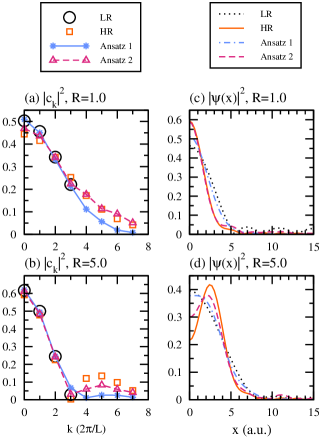
Figure 8: The lowest occupied Hartree-Fock wavefunction of the triplet ground state of H₂ at bond length $R=1.0$ a.u. (a, c) and $R=5.0$ a.u. (b, d) at $L=30$ a.u. for $N_{\textrm{pw}}:7\to 15$ resolution enhancement.

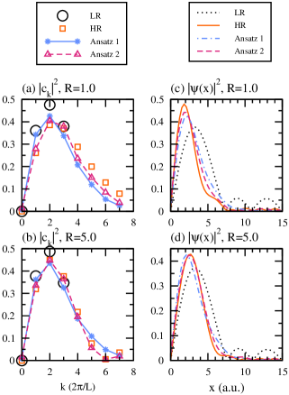
Figure 9: The second lowest occupied Hartree-Fock wavefunction of the triplet ground state of H₂ at bond length $R=1.0$ a.u. (a, c) and $R=5.0$ a.u. (b, d) at $L=30$ a.u. for $N_{\textrm{pw}}:7\to 15$ resolution enhancement.

In order to investigate the qualitative difference between the results of the two ansatzes, in Fig. 7 (a–d) we show the results of case (i) for the singlet ground state of the H₂ molecule at two bond lengths, $R=1.0$ and $R=5.0$. In the Fourier space (Fig. 7 (a, b)), both ansatzes extrapolate the LR wavefunction coefficients $C^{\textrm{LR}}_{k_{j}\mu}$ from the LR region ($k\leq 3$), but only ansatz 2 reproduces a subpeak centered at around $k=5$ in the $R=5.0$ result (Fig. 7 (b)). Ansatz 1 fails to reproduce this structure, and because of the absence of this peak in the Fourier space, the peak of the real-space wavefunction at $x=\pm\frac{R}{2}=2.5$ in Fig. 7 (d) is not reproduced. Similar results are obtained for the two occupied wavefunctions of the triplet H₂, shown in Fig. 8 and Fig. 9, where ansatz 2 better approximates the “tail” region (i.e. $k>3$) and only ansatz 2 can reproduce a subpeak in Fig. 8 (b), although the agreement is not as good as the singlet case. The calculated fidelity values for ansatz 1 (ansatz 2) for the singlet (Fig. 7 (b)) and lowest triplet (Fig. 8 (b)) orbitals at $R=5.0$ are 0.974 (0.996) and 0.930 (0.978), respectively.

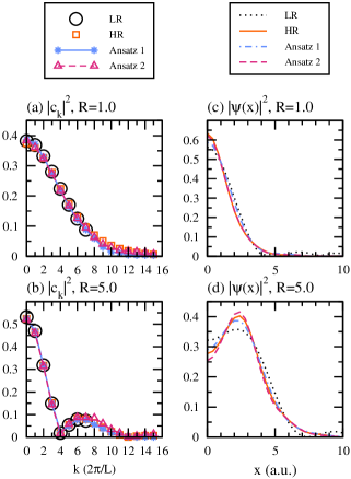
Figure 10: The occupied Hartree-Fock wavefunctions of the singlet ground state of H₂ at bond length $R=1.0$ a.u. (a, c) and $R=5.0$ a.u. (b, d) in Fourier space (a, b) and in real space (c, d) with $L=40$ a.u. for $N_{\textrm{pw}}:15\to 31$ resolution enhancement.

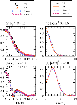
Figure 11: The lowest occupied Hartree-Fock wavefunctions of the triplet H₂ at bond length $R=1.0$ a.u. (a, c) and $R=5.0$ a.u. (b, d) in Fourier space (a, b) and in real space (c, d) with $L=40$ a.u. for $N_{\textrm{pw}}:15\to 31$ resolution enhancement.

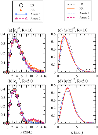
Figure 12: The second lowest occupied Hartree-Fock wavefunctions of the triplet H₂ at bond length $R=1.0$ a.u. (a, c) and $R=5.0$ a.u. (b, d) in Fourier space (a, b) and in real space (c, d) with $L=40$ a.u. for $N_{\textrm{pw}}:15\to 31$ resolution enhancement.

Figures 10–12 show the results of the H₂ molecule in case (ii). In this case the LR Fourier wavevectors cover a wider region ($k\leq 7$) and the contribution from the tail region ($k>7$) is small, but one can still see that ansatz 2 shows a better agreement with the HR wavefunctions.

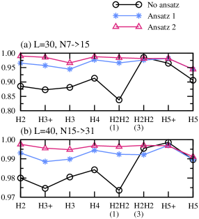
Figure 13: Calculated average fidelity values for the validation dataset. The numbers in the parentheses of the H₂H₂ labels indicate the bond length of the two H₂ molecules.

Figure 13 shows the average fidelity values for each species included in the validation data (Table 3). The validation dataset contains samples for molecules and cations not included in the training data, namely H${}_{3}^{+}$, H₂-H₂(two H₂ molecules), H${}_{5}^{+}$, and H₅. One can see the same overall trend as the training data, where both ansatzes improve the fidelity, and ansatz 2 generally gives higher fidelity values. Larger disagreements are seen in H₃ for case (i) and H₅, both of which have odd numbers of electrons.

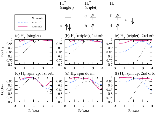
Figure 14: Fidelity values of the occupied wavefunctions of H${}^{+}_{3}$(a–c) and H₃(d–f) for various bond lengths for $N_{\textrm{pw}}:7\to 15$ resolution enhancement at $L=30$.

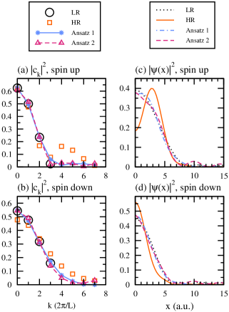
Figure 15: The two lowest Hartree-Fock wavefunctions of H₃ at bond length $R=3.0$ at $L=30$ for $N_{\textrm{pw}}:7\to 15$ resolution enhancement. (a) the lowest occupied spin-up (majority spin) wavefunction, (b) the occupied spin-down (minority spin) wavefunction.

To analyze the obtained results, in Fig. 14 we plot orbital-dependent fidelity values of H${}^{+}_{3}$ and H₃ for case (i) as a function of bond length $R$. One can see that the LR wavefunctions without including an ansatz, shown with dashed lines, generally have low fidelity values for small $R$, due to the fact that in the LR calculation the atomic positions cannot be properly resolved in this region. In fact, small $R$ seems to be the main domain where the current QML models are the most effective. Ansatz 2 yields higher fidelity values for the three H${}^{+}_{3}$ orbitals (Fig. 14 (a–c)) and the highest orbital of H₃ (Fig. 14 (f)) for all $R$, but large discrepancies are seen in the lowest two orbitals of H₃ (Fig. 14 (d, e)) for large $R$. In Fig. 15 we plot these two wavefunctions at $R=3.0$. While the HR curves of the two orbitals in the Fourier space (squares in Fig. 15 (a, b)) have qualitatively different shapes especially for $k>3$, the LR curves (open circles), whose domain is $k\leq 3$, are fairly similar, making the prediction of distinct extrapolations rather challenging. One possible way to improve the results is to include the spin dependence in the effective potential used in Eq. (9) for ansatz 2. This point is left for future research.

H₅ is the largest molecule in the current dataset and is also the system where our models perform the poorest. The reason for the low fidelity values may partly be due to the spin-dependence not included in our ansatz as in the H₃ case, and also because of its electron configuration. H₅ contains five occupied (spin) orbitals, with the highest one having a distinctive spatial character that is not well represented in the training dataset. Adding training data with this configuration would be required to improve the prediction performance on H₅. Interestingly, the fidelity is higher for H${}_{5}^{+}$ and also for two H₂ (H₂H₂), which have the same electron configuration as H₄ and has no spin polarization. These results suggest that the accuracy is more affected by the electronic configuration of the system than by the atomic positions.

Our results indicate that ansatz 2 shows a good predictive power not only for the systems in the training dataset, but also for those which were not present in the dataset, except when the electron configuration is significantly underrepresented in the training dataset. It may be interesting to interpret this ansatz in the context of quantum optimal control (QOC) theory [39, 40, 41]; QOC theory considers a unitary time propagator with an effective Hamiltonian $e^{-iH_{\textrm{eff}}t}$, where $H_{\textrm{eff}}$ consists of the system Hamiltonian and the time-dependent drift or control Hamiltonian. The latter Hamiltonian steers a given system to some desired state, which in the current case is the true HR wavefunction. Our ansatz 2, given by Eq. (9), may be regarded as a QOC time propagator with $N_{l}$ discretized time steps, where the potential term of the system Hamiltonian is explicitly included, and the second part $(U_{\textrm{HEA}})$ takes into account the rest of the system Hamiltonian and also the (system-dependent) drift term. Adding more layers in the ansatz corresponds to increasing the evolution time or reducing the time step in the propagation, which is expected to give improved results. One may be able to reduce the number of parameters in the ansatz by explicitly including the kinetic energy term. It could also be possible to simplify the training algorithm with the help of quantum optimal control techniques, such as the gradient ascent pulse engineering (GRAPE) algorithm [42].

III.2 Two-electron case

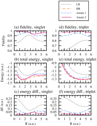
Figure 16: Results of $N_{\textrm{pw}}:7\to 15$ enhancement for the two-electron wavefunctions of the H₂ molecule at $L=30$ a.u. as a function of the bond length $R$ for the singlet state (a, b, c) and the triplet state (d, e, f). (a) and (d) show the fidelity values between true $HR$ and predicted wavefunctions, (b) and (e) show the total energies, and (c, f) are energy differences from HR results, $\Delta E=|E-E_{\textrm{HR}}|$.

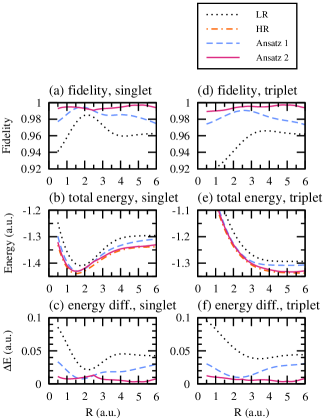
Figure 17: Same as Fig. 16 but for $N_{\textrm{pw}}:15\to 31$ resolution enhancement at $L=40$.

To further investigate the performance of the trained models, we apply the trained models to generate interacting HR two-electron wavefunctions of the H₂ molecule from the LR wavefunctions, using the approach explained in the previous section. We consider the spatial part of two-electron wavefunctions in spin singlet ($s$) and triplet ($t$) states

$$|\Psi^{s,t}_{2}\rangle=\sum_{k_{0}k_{1}}C^{s,t}_{k_{0}k_{1}}|k_{0}k_{1}\rangle,$$ (16)

where the expansion coefficients satisfy the following symmetry properties:

$$C^{s}_{k_{0}k_{1}} = +C^{s}_{k_{1}k_{0}},$$ (17)

$$C^{t}_{k_{0}k_{1}} = -C^{t}_{k_{1}k_{0}}.$$ (18)

In Figs. 16 (a, d) and Figs. 17 (a, d), the calculated fidelities are shown for various bond lengths. It can be seen that as in the one-particle case, both of the trained models (ansatzes 1 and 2) generate wavefunctions with higher fidelity values with the true HR wavefunctions, and ansatz 2 again yields better results. Near the equilibrium bond length ($R\approx 1.5$ a.u.), the wavefunction can be approximated by a single Slater determinant, and by neglecting the antisymmetry of the wavefunctions the fidelity values of the two-body wavefunctions $f$ can be estimated from those of the one-particle orbitals in the wavefunction $f_{\mu\sigma}$ as $f\approx\prod_{\mu\sigma}^{\textrm{occupied}}f_{\mu\sigma}$. For case (i) (Fig. 16), the estimated fidelity values of the singlet (triplet) H₂ at $R=1.0$ are 0.925 (0.900) and 0.991 (0.971) for ansatz 1 and 2, respectively, and for case (ii) (Fig. 17) they are 0.987 (0.980) and 0.997 (0.990) for ansatz 1 and 2, respectively. The fidelity in ansatz 1 decreases for larger $R$ in both cases, which again indicates the limitation of a linear ansatz for this problem. This error originates from the inaccuracy of the one-particle model $U(\bm{\theta})$ for larger $R$ as shown in, for example, one-particle data in Fig. 8 (b).

In Fig. 16 and Fig. 17 we also compute the total energy of H₂, calculated as the expectation value of the following first-quantized Hamiltonian [31]

$$H = \sum_{i_{\textrm{el}}}^{2}\sum_{k,k^{\prime}}\Bigl{[}\delta_{kk^{\prime}}\frac{k^{2}}{2}|k\rangle\langle k|_{i_{\textrm{el}}}$$ (19)

$$-\sum_{I}^{N_{\textrm{nuc}}}Z_{I}e^{-i(k-k^{\prime})d_{I}}\tilde{v}_{\textrm{exp}}(k-k^{\prime})|k\rangle\langle k^{\prime}|_{i_{\textrm{el}}}\Bigr{]}$$

$$+\frac{1}{2}\sum_{i_{\textrm{el}}\neq i_{\textrm{el}}^{\prime}}^{2}\sum_{q,k,k^{\prime}}\Bigl{[}\tilde{v}_{\textrm{exp}}(q)|k-q\rangle\langle k|_{i_{\textrm{el}}}|k^{\prime}+q\rangle\langle k^{\prime}|_{i_{\textrm{el}}^{\prime}}\Bigr{]}$$

$$+E_{\textrm{nn}},$$

where $i_{\textrm{el}},i_{\textrm{el}}^{\prime}$ are the electron indices and $|k\rangle\langle k|_{i_{\textrm{el}}}$ act on the $i_{\textrm{el}}$-th register. The remainder of the equation is explained in Appendix A. Although we do not optimize wavefunctions by minimizing the energy expectation values, the calculated total energies with the generated wavefunctions are closer to the HR values.

It is interesting that this approach, using the models trained with one-particle wavefunctions, also works for many-body wavefunctions, especially for larger $R$, where the wavefunctions have a multi-reference character (i.e. wavefunctions are more strongly entangled) and mean-field approaches like the Hartree-Fock approximation become invalid. This suggests one potential future application of the current approach, which is to generate approximate many-body wavefunctions with low computational cost by using a model $U(\bm{\theta},\mathbf{D}^{(i)})$ trained with one-particle wavefunctions, which can be obtained efficiently with classical computers.

IV conclusions

We performed a numerical experiment of quantum machine learning with quantum input data, where one-particle wavefunctions expanded in the plane-wave basis are generated from those composed from a smaller number of basis functions. The results were improved significantly by including sample-dependent information in the ansatz, suggesting the importance of nonlinearity in the ansatz for this problem. The trained models yielded reasonable results also for molecular structures not included in the training dataset, although they do not generalize enough to generate HR wavefunctions with unseen electronic configurations. Possible pathways to improve the generalizability have been identified. We also showed that the trained models can be used to enhance the resolution of two-electron wavefunctions, and that many-body correction is required for a scalable generalization of the current approach to many-body wavefunctions.

The current work provides one QML example where a data re-uploading-like ansatz is successfully combined with quantum input, by injecting data-dependent classical information into the ansatz. It may be interesting to see if a similar improvement can be achieved in other cases, when some auxiliary data-dependent information is available.

One may think of potential applications of this approach in various directions, such as the generation of all-electron wavefunctions from pseudo wavefunctions in pseudo-potential-based calculations [27].

Appendix A Plane-wave basis

We consider the following one-dimensional Hamiltonian for $N_{\textrm{el}}$ electrons in the presence of $N_{\textrm{nuc}}$ nuclei

$$H = \sum_{i=1}^{N_{\textrm{el}}}\Bigl{[}-\frac{1}{2}\frac{d^{2}}{dx_{i}^{2}}+v_{\textrm{en}}(x_{i})\Bigr{]}+\sum_{i<j}^{N_{\textrm{el}}}V_{\textrm{ee}}(x_{i}-x_{j})$$ (20)

$$+E_{\textrm{nn}},$$

where $v_{\textrm{en}}(x)$ is the attractive Coulomb potential between the electrons and the nuclei, $V_{\textrm{ee}}(|x_{i}-x_{j}|)$ is the repulsive Coulomb potential between the electrons, and $E_{\textrm{nn}}$ is the Coulomb potential between the nuclei, which is a constant under the Born-Oppenheimer approximation. We use atomic units throughout. The explicit forms of these terms are

$$v_{\textrm{en}}(x)=\sum_{I}^{N_{\textrm{nuc}}}-Z_{I}v_{\textrm{exp}}(x-d_{I}),$$ (21)

$$V_{\textrm{ee}}(x)=v_{\textrm{exp}}(x),$$ (22)

$$E_{\textrm{nn}}=\sum_{I<J}Z_{I}Z_{J}v_{\textrm{exp}}(d_{I}-d_{J}).$$ (23)

Here $Z_{I}$ and $d_{I}$ are respectively the atomic number and the position of nucleus $I$, and $v_{\textrm{exp}}(x)$ is the exponential Coulomb-mimicking potential proposed in Ref. [34]

$$v_{\textrm{exp}}(x)=A\exp(-\kappa|x|)$$ (24)

with $A=1.071295$ and $\kappa=1/2.385345$.

The Hartree-Fock one-particle Hamiltonian in Eq. (4) for spin $\sigma$$(=\uparrow,\downarrow)$ is given as

$$h^{\textrm{HF}\sigma}_{jj^{\prime}} = \langle\chi_{k_{j}}|h^{\textrm{HF}\sigma}|\chi_{k_{j^{\prime}}}\rangle$$ (25)

$$= h^{0}_{jj^{\prime}}+\sum_{\sigma^{\prime}}\sum_{ll^{\prime}}D_{ll^{\prime}}^{\sigma^{\prime}}\Bigl{[}V_{jj^{\prime}l^{\prime}l}-\delta_{\sigma\sigma^{\prime}}V_{jll^{\prime}j^{\prime}}\Bigr{]},$$

where

$$h^{0}_{jj^{\prime}} = \delta_{k_{j}k_{j^{\prime}}}\frac{k_{j}^{2}}{2}$$ (26)

$$-\sum_{I}^{N_{\textrm{nuc}}}Z_{I}e^{i(k_{j}-k_{j^{\prime}})d_{I}}\tilde{v}_{\textrm{exp}}(k_{j}-k_{j^{\prime}}),$$

$$D_{ll^{\prime}}^{\sigma}=\sum_{\mu}^{\textrm{occupied}}C_{k_{l}\mu\sigma}C^{*}_{k_{l^{\prime}}\mu\sigma},$$ (27)

$$V_{jj^{\prime}ll^{\prime}}=\delta_{k_{j}+k_{j^{\prime}},k_{l}+k_{l^{\prime}}}\tilde{v}_{\textrm{exp}}(k_{l}-k_{l^{\prime}}).$$ (28)

Here $\tilde{v}_{\textrm{exp}}(k)$ are the Fourier components of $v_{\textrm{exp}}(x)$

$$\tilde{v}_{\textrm{exp}}(k)=\frac{2A\kappa}{L(\kappa^{2}+k^{2})}.$$ (29)

Appendix B Dataset

We prepare one-particle wavefunctions of $H_{x}$ molecules ($x=1,2,3,4,5$) and cations in the spin-restricted Hartree-Fock (RHF) or unrestricted Hartree-Fock (UHF) approximations, which are summarized in Tables 2 and 3 for the training and the validation datasets, respectively.

	method	$N_{\textrm{orb}}$	$R$ (a.u.)
H2 (singlet)	RHF	1	[1.0, 2.0, 3.0, 4.0, 5.0, 6.0]
H2 (triplet)	UHF	2	[1.0, 2.0, 3.0, 4.0, 5.0, 6.0]
H3	UHF	3	[1.0, 2.0, 3.0, 4.0]
H4	RHF	2	[1.0, 2.0, 3.0, 4.0]

Table 2: Training dataset used in this work. Here $N_{\textrm{orb}}$ is the number of orbitals used and $R$ is a bond length. All H atoms are equidistantly aligned.

	method	$N_{\textrm{orb}}$	$R$ (a.u.)
H2 (singlet)	RHF	1	[0.5, 0.5625, 0.625, $\cdots$, 6.0]
H2 (triplet)	UHF	2	[0.5, 0.5625, 0.625, $\cdots$, 6.0]
H${}^{+}_{3}$ (singlet)	RHF	1	[0.5, 0.5625, 0.625, $\cdots$, 4.0]
H${}^{+}_{3}$ (triplet)	UHF	2	[0.5, 0.5625, 0.625, $\cdots$, 4.0]
H3	UHF	3	[0.5, 0.5625, 0.625, $\cdots$, 4.0]
H4	RHF	2	[0.5, 0.5625, 0.625, $\cdots$, 4.0]
H2-H2	RHF	2	[0.5, 0.5625, 0.625, $\cdots$, 4.0]
H${}_{5}^{+}$	RHF	2	[1.5, 1.5625, 1.625, $\cdots$, 3.0]
H5	UHF	5	[1.5, 1.5625, 1.625, $\cdots$, 3.0]

Table 3: Validation dataset used in this work. All H atoms are aligned equidistantly except in H₂-H₂, where $R$ indicates the distance between two H₂ molecules with bond length $R^{\prime}$.

We preprocess the phase of the training dataset so that $C_{k_{0}\mu\sigma}>0$ is satisfied for all the LR and HR wavefunction coefficients, where $k_{0}=\frac{2\pi}{L}$ is an arbitrarily chosen wavevector. For the molecules in the training data with $N_{\textrm{orb}}\geq 2$ (H₂(triplet), H₃ and H₄), we additionally include $\psi_{\mu_{12}\sigma}=\frac{1}{\sqrt{2}}\bigl{[}\psi_{\mu_{1}\sigma}+\psi_{\mu_{2}\sigma}\bigr{]}$ in the training datasets to align the phases of the predicted HR wavefunctions, as explained in the main text.

Appendix C Linear interpolation

Figure 18: Quantum circuit for the linear interpolation. The states with $0$ in the ancilla qubit (bottom) are post-selected. Here $\theta_{0}=2\arctan(\frac{1}{\sqrt{2}})$.

We consider a linear interpolation of a one-dimensional vector $f\in\mathbb{C}^{N}$ encoded in the amplitudes of $n=\log_{2}N$ qubit state as $f=\sum_{j=0}^{N-1}f_{j}|j\rangle=\sum_{j_{0},j_{1},\dots,j_{n-1}}f_{j_{0}j_{1}\dots j_{n-1}}|j_{0}\rangle\otimes\dots\otimes|j_{n-1}\rangle$, where $j=j_{n-1}+2j_{n-2}+\cdots+2^{n-2}j_{1}+2^{n-1}j_{0}$. Our objective is to generate $2N$ states with $n+1$ qubits as

$$\sum_{j=0}^{N-1}f_{j}|j\rangle\otimes|0\rangle$$

$$\to\mathcal{N}\sum_{j=0}^{N-1}\Bigl{[}f_{j}|j\rangle|0\rangle+\frac{f_{j}+f_{j+1}}{2}|j\rangle|1\rangle\Bigr{]},$$ (30)

where $\mathcal{N}$ is a normalization factor, and we define $f_{N}=f_{0}$ (periodic boundary condition). We perform the linear interpolation of the one-particle wavefunctions $\{\psi_{\mu\sigma}\}$ in real space with one ancilla qubit, using the quantum circuit shown in Fig. 18. The first QFT transforms the wavefunctions to real space, and $U(j\to j-1)$ is an operator that shifts $|j\rangle$ to $|j-1\rangle$ ($|-1\rangle=|N-1\rangle$), which can be implemented as described in Ref. [43]. It should be noted that this interpolation breaks the orthonormality of the interpolated wavefunctions.

References

- [1] M. Schuld, I. Sinayskiy, and F. Petruccione, Contemporary Physics 56, 172 (2015).
- [2] J. Biamonte, P. Wittek, N. Pancotti, P. Rebentrost, N. Wiebe, and S. Lloyd, Nature 549, 195 (2017).
- [3] M. Cerezo, A. Arrasmith, R. Babbush, S. C. Benjamin, S. Endo, K. Fujii, J. R. McClean, K. Mitarai, X, Yuan, L. Cincio, and P. J. Coles, Nature Reviews Physics 3, 625 (2021).
- [4] P. Rebentrost, M. Mohseni, and S. Lloyd, Phys. Rev. Lett. 113, 130503 (2014).
- [5] Y. Liu, S. Arunachalam, and K. Temme, Nature Physics 17, 1013 (2021).
- [6] H.-Y. Huang, M. Broughton, M. Mohseni, R. Babbush, S. Boixo, H. Neven, and J. R. McClean, Nature Communications 12, 2631 (2021).
- [7] M. Schuld and N. Killoran, arXiv:2203.01340.
- [8] J. M. Kübler, S. Buchholz, and B. Schölkopf, arXiv:2106.03747.
- [9] Y. Qian, X. Wang, Y. Du, X. Wu, and D. Tao, arXiv:2106.04975.
- [10] E. Perrier, A. Youssry, and C. Ferrie, arXiv:2108.06661.
- [11] L. Schatzki, A. Arrasmith, P. J. Coles, and M. Cerezo, arXiv:2109.03400.
- [12] I. Cong, S. Choi, and M. D. Lukin, Nature Physics 15, 1273 (2019).
- [13] A. V. Uvarov, A. S. Kardashin, and J. D. Biamonte, Phys. Rev. A 102, 012415 (2020).
- [14] L. Banchi, J. Pereira, and S. Pirandola, arXiv:2102.08991.
- [15] N. Wrobel, A. Baul, J. Moreno, and K.-M. Tam, arXiv:2111.05076.
- [16] J. Romero, J. P. Olson, and A. Aspuru-Guzik, Quantum Science and Technology 2, 045001 (2017).
- [17] M. Bilkis, M. Cerezo, G. Verdon, P. J. Coles, and L. Cincio, arXiv:2103.06712 (2022).
- [18] M. Schuld and N. Killoran, Phys. Rev. Lett. 122, 040504 (2019).
- [19] M. Schuld and F. Petruccione, Supervised Learning with Quantum Computers, 1st ed. (Springer, 2018).
- [20] A. Péres-Salinas, A. Cervera-Lierta, E. GilFuster, and J. I. Latorre, Quantum 4, 226 (2020).
- [21] J. G. Vidal and D. O. Theis, Front. Phys. 8, 297 (2020).
- [22] M. Schuld, R. Sweke, and J. J. Meyer, Phys. Rev. A 103, 032430 (2021).
- [23] W. Yang, X. Zhang, Y. Tian, W. Wang, J. Xue and Q. Liao, IEEE Transactions on Multimedia, vol. 21, no. 12, pp. 3106–3121 (2019).
- [24] S. M. A. Bashir, Y. Wang, M. Khan, and Y. Niu, PeerJ Comput. Sci. 7:e621 DOI 10.7717/peerj-cs.621 (2021).
- [25] C. Dong, C. C. Loy, K. He, and X. Tang, in Proceedings of the European Conference on Computer Vision, pp. 184–199 (2014).
- [26] C. Ledig et al., IEEE Conference on Computer Vision and Pattern Recognition (CVPR), pp. 105–114 (2017).
- [27] R. M. Martin, Electronic Structure: Basic Theory and Practical Methods (Cambridge University Press, 2004).
- [28] D. W. Berry, M. Kieferová, A. Scherer, Y. R. Sanders, G. H. Low, N. Wiebe, C. Gidney, and R. Babbush, npj Quantum Information 4, 22 (2018).
- [29] R. Babbush, N. Wiebe, J. McClean, J. McClain, H. Neven, and G. K.-L. Chan, Phys. Rev. X 8, 011044 (2018).
- [30] R. Babbush, D. W. Berry, J. R. McClean, and H. Neven, npj Quantum Information 5, 92 (2019).
- [31] Y. Su, D. W. Berry, N. Wiebe, N. Rubin, and R. Babbush, PRX Quantum 2, 040332 (2021).
- [32] T. E. O’Brien, M. Streif, N. C. Rubin, R. Santagati, Y. Su, W. J. Huggins, J. J. Goings, N. Moll, E. Kyoseva, M. Degroote, C. S. Tautermann, J. Lee, D. W. Berry, N. Wiebe, and R. Babbush, arXiv:2111.12437.
- [33] A. Delgado, P. A. M. Casares, R. dos Reis, M. S. Zini, R. Campos, N. Cruz-Hernández, A.-C. Voigt, A. Lowe, S. Jahangiri, M. A. Martin-Delgado, J. E. Mueller, and J. M. Arrazola, arXiv:2204.11890.
- [34] T. E. Baker, E. M. Stoudenmire, L. O. Wagner, K. Burke, and S. R. White, Phys. Rev. B 91, 235141 (2015).
- [35] L. Li, S. Hoyer, R. Pederson, R. Sun, E. D. Cubuk, P. Riley, and K. Burke, Phys. Rev. Lett. 126, 036401 (2021).
- [36] W. H. Press, S. A. Teukolsky, W. T. Vetterling, and B. P. Flannery, Numerical Recipes in C, 3rd ed. (Cambridge University Press, Cambridge, 2007).
- [37] A. Choquette, A. Di Paolo, P. K. Barkoutsos, D. Sénéchal, I. Tavernelli, and A. Blais, Phys. Rev. Res. 3, 023092 (2021).
- [38] V. Bergholm, J. Izaac, M. Schuld, C. Gogolin, C. Blank, K. McKiernan, and N. Killoran, arXiv:1811.04968.
- [39] J. Werschnik and E. K. U. Gross, Journal of Physics B: At. Mol. Opt. Phys. 40, R175 (2007).
- [40] S. J. Glaser, U. Boscain, T. Calarco, C. P. Koch, W. Köckenberger, R. Kosloff, I. Kuprov, B. Luy, S. Schirmer, T. Schulte-Herbrüggen, D. Sugny, and F. K. Wilhelm, Eur. Phys. J. D 69, 279 (2015).
- [41] T. S. Mahesh, P. Batra, and M. H. Ram, arXiv:2205.15574.
- [42] N. Khaneja, T. Reiss, C. Kehlet, T. S. Herbrüggen, and S. J. Glaser, J. Magn. Reson. 172, 296 (2005).
- [43] P. Fan, R.-G. Zhou, N. Jing, and H.-S. Li, Information Sciences 340–341, 191 (2016).