Simulation-Based Parallel Training

Abstract

Numerical simulations are ubiquitous in science and engineering. Machine learning for science investigates how artificial neural architectures can learn from these simulations to speed up scientific discovery and engineering processes. Most of these architectures are trained in a supervised manner. They require tremendous amounts of data from simulations that are slow to generate and memory greedy. In this article, we present our ongoing work to design a training framework that alleviates those bottlenecks. It generates data in parallel with the training process. Such simultaneity induces a bias in the data available during the training. We present a strategy to mitigate this bias with a memory buffer. We test our framework on the multi-parametric Lorenz’s attractor. We show the benefit of our framework compared to offline training and the success of our data bias mitigation strategy to capture the complex chaotic dynamics of the system.

1 Introduction

Multiparametric dynamical simulations are crucial to scientific discovery and engineering applications from computational fluid dynamics [30] to biochemistry [1]. Let’s denote $g$ such a simulation, $X$ its input parameters and $Y^{t}_{X}$ the output for a given time step $t$.

$$g\colon\mathbb{R}^{d_{\text{in}}} \to\mathbb{R}^{d_{\text{out}}\times T}$$

$$X \mapsto\{Y^{t}_{X},t\in[0,T],T\in\mathbb{R}^{+}\}$$

Recently, scientists have considered deep learning as a means to accelerate science by speeding up those simulations and learning from them [37]. Most works train an artificial neural network $f_{\theta}$ in a supervised manner, from data generated by the simulation process $g$. The exact combination of inputs and outputs of the training process depends on the application. For instance, for a network trained to replace the original simulator $g$ with direct time predictions, as done in the seminal work of Raissi et al. [33], we have $f_{\theta}(X,t)\approx Y^{t}_{X}$. However, for the auto-regressive models proposed in [32, 4], we have $f_{\theta}(X,Y^{t}_{X})\approx Y^{t+1}_{X}$.

Classical training consists in generating a set of simulation data $\mathcal{X}_{\text{train}}$, $\mathcal{Y}_{\text{train}}$. Where $\mathcal{X}_{\text{train}}$ would be representative of a parameter set on which we want to infer with the trained neural network. Efficient training $f_{\theta}$, and capturing all the complexity of the simulated system, generally requires tremendous amounts of data [6]. The dimension of $\mathcal{Y}_{\text{train}}$ can thus quickly explode and lead to a massive memory footprint. Additionally, the sequential generation of $\mathcal{Y}_{\text{train}}$ can be prohibitively slow. To overcome these limitations, one may restrict $\mathcal{X}_{\text{train}}$, or subsample $\mathcal{Y}_{\text{train}}$ by reducing the number of time steps or observed dimensions. To reduce $\mathcal{X}_{\text{train}}$ does not necessarily hinder the quality of the training. Techniques ranging from adaptive experimental design [12] to importance sampling [17] help to identify the parameters that will bring the most relevant information for the training of the network. These techniques, however, require knowledge about the network response to different inputs $X$, which is not feasible if $\mathcal{X}_{\text{train}}$ is set beforehand.

We propose a framework that generates the simulation data simultaneously with the training process. Data generation is highly parallelized and streamed to training to avoid storing any data in files. The framework also allows the steering of the training by selecting new parameters $X$ based on some feedback from the network on previously presented parameters. This article presents our ongoing work covering the first point. Compared to classical training from files, the simultaneity of the training and the data generation presents specificities that must be addressed.

At any time $\tau$ of the training process, only the already generated data $\mathcal{Y}^{\tau}$ can be presented to the network. There is no guarantee that $\mathcal{Y}^{\tau}$ is representative of $\mathcal{Y}_{\text{train}}$. Because of the limited number of concurrent simulations $g$ and their iterative production of data, the two sets can have very distinct distributions. This setting commonly arises in online deep learning [8]. If we stream the data, using the last received time step $Y^{\tau}$ directly for training, this is known to lead to poor performances related to catastrophic forgetting [18]. Therefore, to mitigate the bias in the data due to the discrepancies between $\mathcal{Y}_{\text{train}}$ and $\mathcal{Y}^{\tau}$, we introduce a memory buffer of limited size. It is associated with a data management policy in charge of the selection of elements to construct batches and their eviction when the buffer is full. Moreover, we rely on a simple sampling strategy of $\mathcal{X}_{\text{train}}$ to improve the diversity of $\mathcal{Y}^{\tau}$.

We validate our framework and the strategy to mitigate data bias on a model that captures the chaotic dynamics of Lorenz’s attractor [26]. First, we show that our data bias mitigation strategy is successful in producing more diverse batches than pure streaming learning. Second, we show that our framework can prevent the overfitting offline training suffers, by exposing the network to more diverse trajectories. This overfitting typically occurs when the simulation data are too big to be stored, which imposes to limit the size of the dataset and consequently reduces its representativeness. Third, we show that the framework can match the performances of offline training with a comprehensive dataset. This illustrates there is no performance decrease using the online framework.

The main contributions of our ongoing work are:

• a deep learning framework orchestrating parallel data simulations with the online training of neural architectures on multi-parametric dynamical systems;

• a strategy to mitigate the bias in data induced by the online nature of the framework.

2 Related Work

2.1 Deep Learning and Numerical Simulations

In recent years, deep learning has permeated the numerical simulations of multi-parametric dynamical systems. Scientists proposed algorithms to substitute the traditional partial differential equations (PDE) solvers [33, 23, 4]. Instead of replacing entirely the original solver, others proposed to augment the resolution of coarse solutions [39, 20]. Similarly, Erichson et al. presented a network to reconstruct the dynamics of a fluid from a few data points only [10]. Others have relied on numerical simulations to study how machine learning interfaces with traditional dynamical system theories, like the Koopman operator [28], or help to rediscover the governing equations of simulated systems [7].

All these approaches rely on supervised training, for which data mostly come from simulators. Even approaches that could theoretically be data-free, like physics-informed neural networks [33], have required simulated data to work successfully on complex physics [27].

Most of the published work is only presented with fairly simple simulations, either in terms of the complexity of the governing equations or by the scale of the problem at stake. Even though some works propose to capture intrinsic properties of the studied physical systems, it is, to our knowledge, not yet clear how deep learning architectures trained on simple problems can scale to larger and more complex ones, common to the industry and today’s scientific challenges. For instance, using graph neural networks, Pfaff et al. could infer dynamics with higher resolution than the one used for training [32]. Equivariance is another example to learn fundamental properties of a system, like symmetries, and thus reduce the amount of data required for training [35].

2.2 Online Training

By generating the simulations along the training process the full dataset is not accessible anymore at all times. In this setting referred to as online learning [8], data presented to the network may be biased. It leads to poor generalization performances, like catastrophic forgetting [18]. Several techniques have been proposed to mitigate this catastrophic forgetting. Either by tuning the loss for the optimal weights of the network not to change dramatically while being trained on new data [19, 21]. Another approach consists in repeating the samples previously shown to the model [14]. Such a strategy has also been successfully applied in the context of deep reinforcement learning and coined as replay buffer by the community [36, 34].

2.3 Parallel Frameworks for Deep Reinforcement Learning

Training frameworks presenting several degrees of parallelism have already been proposed by the deep reinforcement learning community [31, 29, 16]. Especially, to achieve the acting and the learning in parallel. Similarly, in our framework, the data generation and the training are parallelized. Liang et al. propose, within the Ray project, a task-based formalism to abstract those different degrees of parallelism for deep reinforcement learning [24]. If some reinforcement learning experiments lead to massive parallel resource usage due to the very large number of actors to run, the simulation itself is not massively parallelized [2]. Indeed, these deep reinforcement learning framework support simulations that are either sequential or multi-threaded, but not scientific PDEs solvers requiring distributed memory parallelization with MPI to address problems at a relevant scale.

Despite the similarity in the parallelism of the data generation and the training, the comparison with deep reinforcement learning has limits. We are not learning to interact with an environment but rather learning the environment itself. Therefore there is no policy, and thus no concept of off-policy. All samples are relevant, although some may bear more useful information for the training of the network. It is also worth mentioning the work of Brace et al., which introduces a parallel framework to select biomolecular simulations to run, but not to train generically architectures on numerical simulations [3].

3 Training Framework

3.1 Architecture Overview

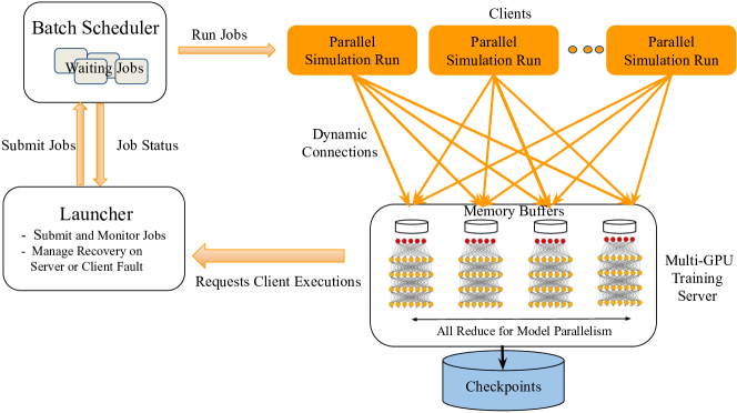
Figure 1: Online Training Framework Overview. The launcher starts and monitors the clients and the server. The server is in charge of the training loop, which can be executed in parallel on several GPUs. It controls the experimental design and requests to the launcher the executions of new client instances for selected sets of parameters. The launcher can start these instances once the batch scheduler has allocated the required compute resources.

Our framework is based on an adaptation of the open source Melissa architecture developed to manage large-scale ensemble runs for sensibility analysis [38] and data assimilation [13]. Our goal is to enable the online (no intermediate storage in files) training of a neural model from data generated through different simulation executions. These simulations are executed with different input parameters (parameter sweep), making the different members of the ensemble.

We target executions on supercomputers where simulations can be large parallel solver codes executed on several nodes and the training parallelized on several GPUs (Figure 1). We give below an overview of the framework, a detailed description being beyond the scope of this paper. The framework relies on three main components:

• The launcher orchestrates the execution of the simulation instances and the training. The launcher interacts with the machine batch scheduler (e.g. Slurm or OAR) to request resources for the other component executions.

• Each client executes one simulation instance. When starting, it dynamically connects to the server. As soon as it produces new data (a new time step), the data is sent to the server.

• The server runs on several GPUs to train the model in parallel. On reception of new data from one client, the data is first pushed into the local memory buffer. When a new batch is required for training, it is extracted from this buffer. The management of this buffer is detailed in the following section 3.2.

This framework thus alleviates the need for files to store intermediate results. We target large-scale executions generating large amounts of data that cannot be reasonably stored. As an example, Melissa has been reported performing a sensibility analysis run executing $8000$ simulation instances that generated $48$TB of data processed online [38]. The secondary benefit of coupling data generation and training is that the server can control which simulation instances to run next, opening the possibility for adaptive experimental design.

The framework combines several levels of parallelism (at the ensemble, client, server, and communication levels) to enable efficient and scalable executions. The simulation can be a parallel code written in C/C++, Fortran or Python, and combining the usage of MPI, OpenMP and Cuda. The server relies on Pytorch Data Distributed Parallelism [22] for enabling multi-GPU training.

3.2 Data Bias Mitigation Strategy

The online data generation inherently carries 3 types of data bias (Figure 2):

• Intra-simulation bias. Simulators produce dynamics as time series by discretizing time and progressing iteratively. After $T$ time steps, only the data $\{Y^{t}_{X},0\leq t\leq T\}$ for the simulation instance $X$ are available for training.

• Inter-simulation bias. Computational resources are limited and so often not all simulation instances can be executed concurrently. Let’s assume that only $c$ simulations can execute concurrently at any time. At the end of the execution of the $c$ first simulations training only has access to the data $\{Y^{t}_{X_{i}},0<i\leq c\}$.

• Memory bias. Not only online training cannot have access to the not already generated data, but we also cannot keep all already generated data due to memory constraints. We can, at most, keep a rolling sample of data that fits into a given memory budget.

Therefore, batches cannot be drawn uniformly from the full dataset as performed with traditional epoch-based training. This bias has a detrimental effect on the training, partly due to catastrophic forgetting [18].

Some physical systems exhibit different behaviors depending on the parameter of the simulation. For instance, Reynolds number for fluid dynamics [11]. The inter-simulation bias creates discrepancies between $\mathcal{Y}^{\tau}$ and $\mathcal{Y}_{\text{train}}$. The sampling strategy consists in selecting parameter $X$ so that $\mathcal{Y}^{\tau}$ is as representative as possible of all the behaviors in $\mathcal{Y}_{\text{train}}$. In the following, we adopt a simple strategy that randomly samples $X$ among $\mathcal{X}_{\text{train}}$.

To mix the data further and address the intra-simulation and memory biases, we introduce a memory buffer. It acts like a cache of the data previously generated and sent to each trainer. Without the memory buffer, data would be immediately streamed from the simulators to the trainers, a situation prone to catastrophic forgetting. The memory buffer has a set capacity, $s$. It is associated with a data management policy that specifies the rule to evict data when the buffer is full, and select data to construct the batches. The current policy selects samples randomly from the buffer and erases them upon selection. This avoids having samples repeated too many times in batches while the trainer is waiting for new data from the simulators. Due to the intra-simulation bias, the first simulation time steps arrive first in the memory buffer. To avoid yielding first batches with overly represented first time steps, we set a threshold $s_{\text{ready}}$ that signals when the buffer has enough elements to be sampled. Because the training loop and the simulation are executed at different speeds on different processes, the memory buffer must also amortize the data production and consumption between the clients and the trainer. We set a second threshold $s_{\text{min}}$ that ensures there is always a minimal amount of samples in the buffer, for the batch construction to be indeed random.

In summary, the key idea is that the simultaneous generation of simulation data creates a bias in the data. We rely on adequate sampling of the simulation parameter and a memory buffer to mix the data presented to the network and guarantee the training quality.

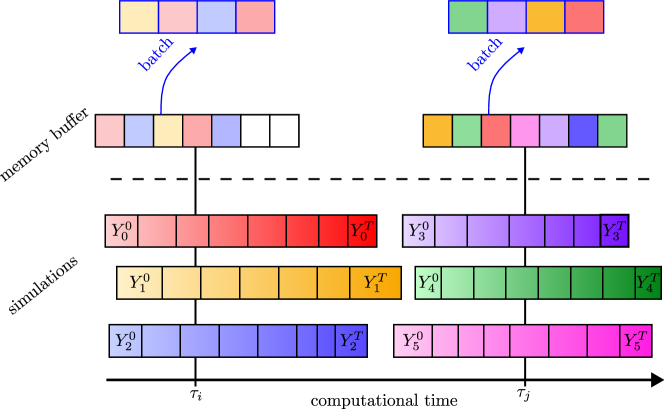
Figure 2: Timeline of the generated simulation data. Here, 3 processes run 6 simulations in parallel. Groups of concurrent simulations are executed sequentially. As soon as a simulation time step $Y^{t}_{X_{i}}$ is computed, it is passed to the memory buffer. Simultaneously, this cache of limited capacity yields batches from previously stored time steps. The content of the buffer and the batches constructed from it are represented at two different times $\tau_{i}$ and $\tau_{j}$. At $\tau_{i}$ the buffer is not yet full. At $\tau_{j}$ the buffer is full and contains some time steps from previous simulations.

4 Experiments

To prove the usefulness of our approach we examine the case of a neural network trained to capture the underlying physics from the observation of complex dynamics. For this purpose, we consider Lorenz’s attractor [26]. Its dynamics are described by the system LABEL:eq:lorenz. The attractor is chaotic. It means that, despite being deterministic, two points initially close have very distinct trajectories. The dynamics thus present a complex and rich behavior. Nonetheless, the underlying non-linear equation is fairly simple. The possibility to recover the dynamics of Lorenz using machine learning techniques has already been studied in [5, 9], even with partial observation [25]. Here, we train a neural network to reconstruct the trajectory with an integration scheme of Euler, i.e. we predict $f_{\theta}(X,Y_{t})\approx\frac{Y_{t+1}-Y_{t}}{\Delta t}$, where $X=\rho$ and $Y_{t}=(x_{t},y_{t},z_{t})$ the coordinates of the system at time $t$ given by Equation LABEL:eq:lorenz. The model is auto-regressive as the trajectory is reconstructed iteratively at inference.

$$\frac{dx}{dt} =\sigma(y-z)$$

$$\frac{dy}{dt} =x(\rho-z)-y$$

$$\frac{dz}{dt} =xy-\beta z$$

We consider the multi-parametric case for which the initial position $X_{0}$ and the parameter $\rho$ vary. $\sigma$ and $\beta$ are respectively fixed to $10$ and $\nicefrac{{8}}{{3}}$. The goal is to train a neural network that generalizes for any initial position and $\rho$ belonging to the interval $[0,100]$. In the following experiments, initial positions $X_{0}$ are always taken from the normal distribution $\mathcal{N}(15,30)$. Data are standardized with statistics computed beforehand. The model architecture also remains the same across the experiments. It consists of 3 layers of 512 features. The first layer has 4 input features for the position and the parameter $\rho$. The output has 3 features for the velocity. We use the SiLU activation function between each intermediate layer [15]. For the memory buffer, we arbitrarily set $s$, $s_{\text{ready}}$, and $s_{\text{min}}$ equivalent to 10, 5 and 3 simulations respectively.

In our experiments, we consider different datasets and training settings. We always generate a different number of trajectories for values of $\rho$ taken in $[0,20,40,60,80,100]$. First, we have a full offline dataset consisting of 100 trajectories of 2000 time steps $\Delta t$ of $10^{-2}$ second. A second offline dataset, we call restricted, consists of only 10 trajectories. A third offline dataset, referred to as subsampled, corresponds to 10000 trajectories sampled every 100 time steps. The restricted and subsampled offline datasets are artificially reduced to illustrate the case of more complex simulations for which it might be difficult to obtain and store a representative dataset. As we compare different dataset sizes and different training strategies (offline or online), for a fair comparison, we ensure that the quantity of information seen by the network is always the same. This translates into a constant total number of batches. For online training, there is no notion of epoch anymore. Hence, the training of the full, restricted, and subsampled datasets is respectively achieved on 100, 1000, and 100 epochs. For the online dataset, we generate 10000 trajectories. In the streaming setting, the trajectories are generated from simulations with increasing values of $\rho$. Data are directly gathered into batches and passed to the trainer. A second online setting, noted as sampling, randomly samples $\rho$ prior to the data generation. The online setting, noted as sampling + memory buffer, combines the random sampling of the parameters and a memory buffer with random data selection policy. For all training strategies, the batch size is fixed to 1024 time steps. The validation dataset consists of 10 trajectories, 2 for each value of $\rho$ taken in the same interval as for the training set.

4.1 Memory Buffer Mitigates the Bias Induced by Online Training

To illustrate the efficiency of the two levels of control, namely the sampling of parameters and the memory buffer, in mitigating the data bias, we consider the batch statistics in the different training settings. Figure 3 shows the mean and standard deviation of the batches for the different strategies. The streaming strategy appears biased, exposing the training process to catastrophic forgetting that can explain the gap between train and validation losses in Figure LABEL:fig:training-strategies. We see that the coupling of the sampling strategy and the memory buffer makes the distribution closer to the one observed in the offline setting, showing its capability to reduce bias.

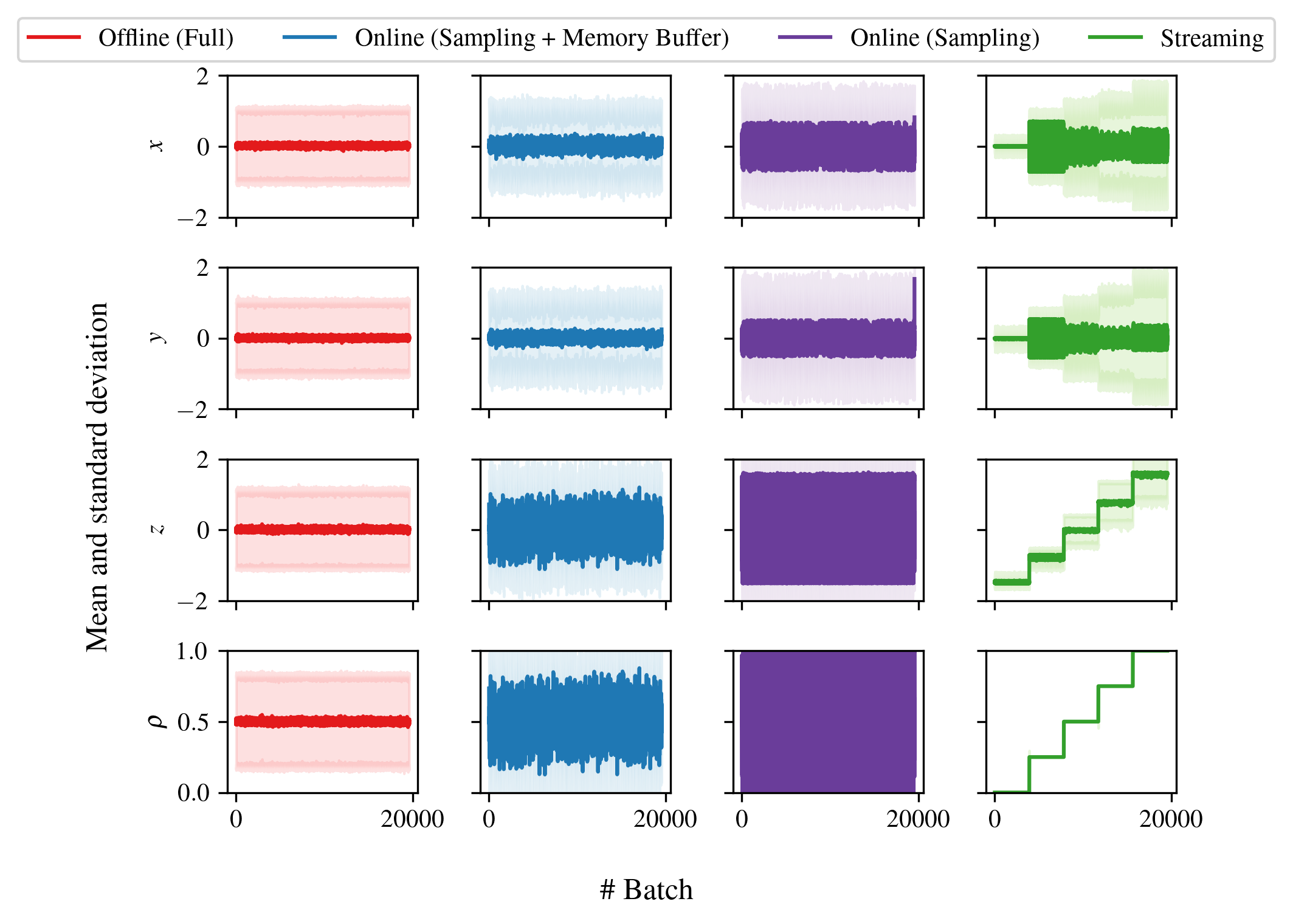
Figure 3: Comparison of batch statistics for different training strategies. Offline training presents batches uniformly drawn from the dataset, which is assumed to lead to the best performances. Sampling and memory buffer correct the prejudicial bias observed in streaming batches.

4.2 Parameter Space Exploration with Online Training

Training and validation losses for the different training settings are displayed in Figure LABEL:fig:training-strategies. We observe that for the restricted and the subsampled offline datasets the validation losses are almost an order higher than the training losses, which indicates overfitting. This shows that, even for simple equations like Lorenz’s system (Equation LABEL:eq:lorenz), a neural network can experience difficulties in recovering the dynamics with only a few trajectories. It stresses the importance of having a representative dataset. For the same number of batches, the online training, with a random sampling strategy and the memory buffer, presents training and validation losses that decrease similarly with the number of batches. It is also for this setting that the validation loss is minimal. By presenting to the network more diverse trajectories, this strategy overcomes the overfitting observed with limited offline datasets.

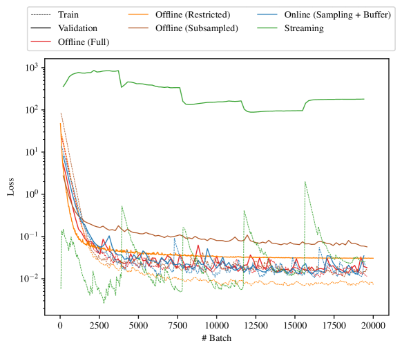
Figure 4: Training and validation in plain and dashed lines respectively for different training strategies.

4.3 Recovery of Offline Performances

Figure LABEL:fig:training-strategies shows the training dynamics with the full offline dataset and the online setting (sampling + buffer) are equivalent. Both configurations correctly recover the dynamics of the attractor on a test trajectory generated with $\rho$ equal to 28 (Figure 5). The predicted trajectories are stable as shown in Figure 5(a). They match the reference for a limited time, as seen in Figure 5(b). The lack of coherence after some time is expected due to the chaotic nature of Lorenz’s attractor. Compared to offline training with a comprehensive dataset, which can be difficult to obtain for more complex systems, the online strategy does not induce any degradation of the trained network performances.

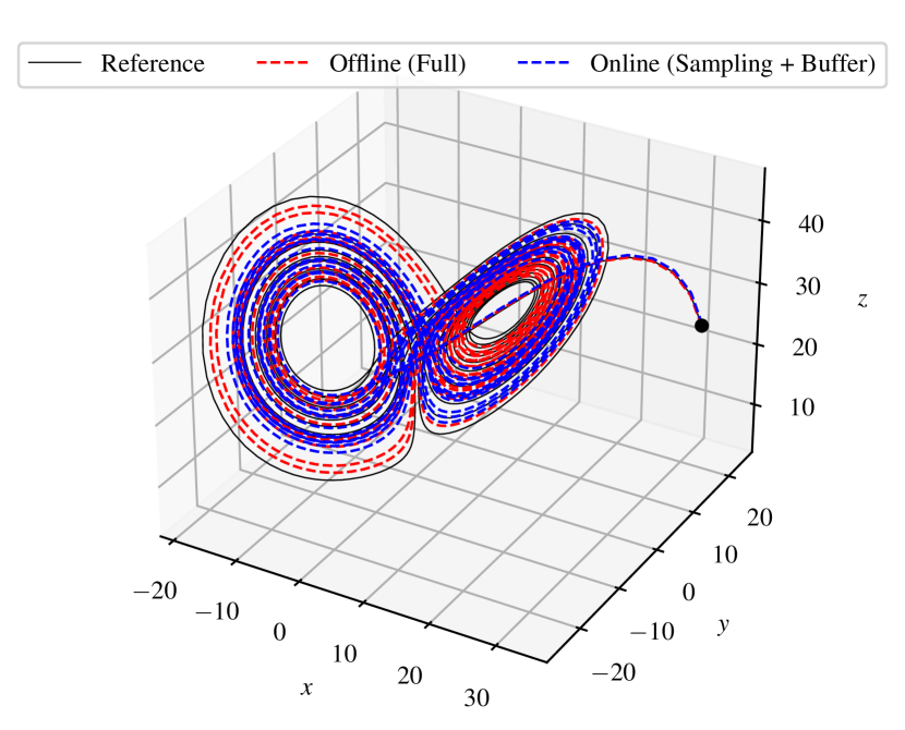
((a)) 3D trajectory

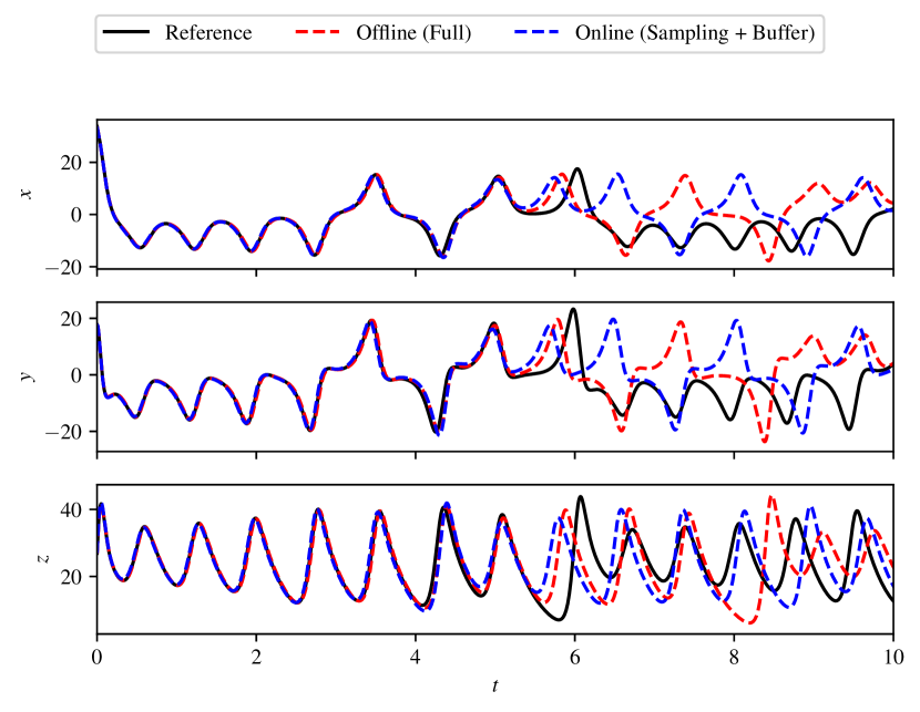
((b)) Per axis trajectory

Figure 5: Comparison of the model predictions on a test trajectory for different training settings. Both settings manage to train the network to accurately capture the dynamics of Lorenz’s attractor.

5 Conclusion

In this article, we have proposed a framework to train artificial neural networks on synthetic simulations generated along the training process. We have shown this setting induces a bias in the data that hinders the quality of the training. We have introduced simple strategies to mitigate the bias: a random sampling of the simulation parameters and a memory buffer that allows mixing further the data presented to the network. We have applied these strategies to train a network on Lorenz’s attractor. We have shown that leveraging the online setting to generate more data, but still keeping the same number of batches as for an offline strategy, can lead to a lower validation loss. We have also shown the strategies were successful to match the performance of offline training with a comprehensive dataset in capturing the underlying dynamics of Lorenz’s atttractor, without incurring the same memory footprint. Such results need further testing with different use cases to be confirmed. Advanced implementations of the memory buffer will also be further investigated like reservoir or importance sampling for the selection of elements in the memory buffer [40, 17].

References

- Abraham et al. [2015] M. J. Abraham, T. Murtola, R. Schulz, S. Páll, J. C. Smith, B. Hess, and E. Lindahl. Gromacs: High performance molecular simulations through multi-level parallelism from laptops to supercomputers. SoftwareX, 1:19–25, 2015.
- Berner et al. [2019] C. Berner, G. Brockman, B. Chan, V. Cheung, P. Dębiak, C. Dennison, D. Farhi, Q. Fischer, S. Hashme, C. Hesse, et al. Dota 2 with large scale deep reinforcement learning. arXiv preprint arXiv:1912.06680, 2019.
- Brace et al. [2022] A. Brace, I. Yakushin, H. Ma, A. Trifan, T. Munson, I. Foster, A. Ramanathan, H. Lee, M. Turilli, and S. Jha. Coupling streaming ai and hpc ensembles to achieve 100–1000 faster biomolecular simulations. In 2022 IEEE International Parallel and Distributed Processing Symposium (IPDPS), pages 806–816. IEEE, 2022.
- Brandstetter et al. [2021] J. Brandstetter, D. E. Worrall, and M. Welling. Message passing neural pde solvers. In International Conference on Learning Representations, 2021.
- Brunton et al. [2016] S. L. Brunton, J. L. Proctor, and J. N. Kutz. Discovering governing equations from data by sparse identification of nonlinear dynamical systems. Proceedings of the national academy of sciences, 113(15):3932–3937, 2016.
- Brunton et al. [2020] S. L. Brunton, B. R. Noack, and P. Koumoutsakos. Machine learning for fluid mechanics. Annual review of fluid mechanics, 52:477–508, 2020.
- Cranmer et al. [2020] M. Cranmer, A. Sanchez Gonzalez, P. Battaglia, R. Xu, K. Cranmer, D. Spergel, and S. Ho. Discovering symbolic models from deep learning with inductive biases. Advances in Neural Information Processing Systems, 33:17429–17442, 2020.
- Ditzler et al. [2015] G. Ditzler, M. Roveri, C. Alippi, and R. Polikar. Learning in nonstationary environments: A survey. IEEE Computational Intelligence Magazine, 10(4):12–25, 2015.
- Dubois et al. [2020] P. Dubois, T. Gomez, L. Planckaert, and L. Perret. Data-driven predictions of the lorenz system. Physica D: Nonlinear Phenomena, 408:132495, 2020.
- Erichson et al. [2020] N. B. Erichson, L. Mathelin, Z. Yao, S. L. Brunton, M. W. Mahoney, and J. N. Kutz. Shallow neural networks for fluid flow reconstruction with limited sensors. Proceedings of the Royal Society A, 476(2238):20200097, 2020.
- Ferziger et al. [2002] J. H. Ferziger, M. Perić, and R. L. Street. Computational methods for fluid dynamics, volume 3. Springer, 2002.
- Foster et al. [2021] A. Foster, D. R. Ivanova, I. Malik, and T. Rainforth. Deep adaptive design: Amortizing sequential bayesian experimental design. In International Conference on Machine Learning, pages 3384–3395. PMLR, 2021.
- Friedemann and Raffin [2022] S. Friedemann and B. Raffin. An elastic framework for ensemble-based large-scale data assimilation. The international journal of high performance computing applications, 36(4):543–563, June 2022. URL https://hal.inria.fr/hal-03017033.
- Hayes et al. [2019] T. L. Hayes, N. D. Cahill, and C. Kanan. Memory efficient experience replay for streaming learning. In 2019 International Conference on Robotics and Automation (ICRA), pages 9769–9776. IEEE, 2019.
- Hendrycks and Gimpel [2016] D. Hendrycks and K. Gimpel. Gaussian error linear units (gelus). arXiv preprint arXiv:1606.08415, 2016.
- Horgan et al. [2018] D. Horgan, J. Quan, D. Budden, G. Barth-Maron, M. Hessel, H. van Hasselt, and D. Silver. Distributed prioritized experience replay. In International Conference on Learning Representations, 2018.
- Katharopoulos and Fleuret [2018] A. Katharopoulos and F. Fleuret. Not all samples are created equal: Deep learning with importance sampling. In International conference on machine learning, pages 2525–2534. PMLR, 2018.
- Kemker et al. [2018] R. Kemker, M. McClure, A. Abitino, T. Hayes, and C. Kanan. Measuring catastrophic forgetting in neural networks. In Proceedings of the AAAI Conference on Artificial Intelligence, volume 32, 2018.
- Kirkpatrick et al. [2017] J. Kirkpatrick, R. Pascanu, N. Rabinowitz, J. Veness, G. Desjardins, A. A. Rusu, K. Milan, J. Quan, T. Ramalho, A. Grabska-Barwinska, et al. Overcoming catastrophic forgetting in neural networks. Proceedings of the national academy of sciences, 114(13):3521–3526, 2017.
- Kochkov et al. [2021] D. Kochkov, J. A. Smith, A. Alieva, Q. Wang, M. P. Brenner, and S. Hoyer. Machine learning–accelerated computational fluid dynamics. Proceedings of the National Academy of Sciences, 118(21):e2101784118, 2021.
- Lee et al. [2017] S.-W. Lee, J.-H. Kim, J. Jun, J.-W. Ha, and B.-T. Zhang. Overcoming catastrophic forgetting by incremental moment matching. Advances in neural information processing systems, 30, 2017.
- Li et al. [2020a] S. Li, Y. Zhao, R. Varma, O. Salpekar, P. Noordhuis, T. Li, A. Paszke, J. Smith, B. Vaughan, P. Damania, et al. Pytorch distributed: Experiences on accelerating data parallel training. arXiv preprint arXiv:2006.15704, 2020a.
- Li et al. [2020b] Z. Li, N. B. Kovachki, K. Azizzadenesheli, K. Bhattacharya, A. Stuart, A. Anandkumar, et al. Fourier neural operator for parametric partial differential equations. In International Conference on Learning Representations, 2020b.
- Liang et al. [2018] E. Liang, R. Liaw, R. Nishihara, P. Moritz, R. Fox, K. Goldberg, J. Gonzalez, M. Jordan, and I. Stoica. Rllib: Abstractions for distributed reinforcement learning. In International Conference on Machine Learning, pages 3053–3062. PMLR, 2018.
- Lin et al. [2021] Y. T. Lin, Y. Tian, D. Livescu, and M. Anghel. Data-driven learning for the mori–zwanzig formalism: A generalization of the koopman learning framework. SIAM Journal on Applied Dynamical Systems, 20(4):2558–2601, 2021.
- Lorenz [1963] E. N. Lorenz. Deterministic nonperiodic flow. Journal of atmospheric sciences, 20(2):130–141, 1963.
- Lucor et al. [2022] D. Lucor, A. Agrawal, and A. Sergent. Simple computational strategies for more effective physics-informed neural networks modeling of turbulent natural convection. Journal of Computational Physics, 456:111022, 2022.
- Lusch et al. [2018] B. Lusch, J. N. Kutz, and S. L. Brunton. Deep learning for universal linear embeddings of nonlinear dynamics. Nature communications, 9(1):1–10, 2018.
- Mnih et al. [2016] V. Mnih, A. P. Badia, M. Mirza, A. Graves, T. Lillicrap, T. Harley, D. Silver, and K. Kavukcuoglu. Asynchronous methods for deep reinforcement learning. In International conference on machine learning, pages 1928–1937. PMLR, 2016.
- Moin and Mahesh [1998] P. Moin and K. Mahesh. Direct numerical simulation: a tool in turbulence research. Annual review of fluid mechanics, 30(1):539–578, 1998.
- Nair et al. [2015] A. Nair, P. Srinivasan, S. Blackwell, C. Alcicek, R. Fearon, A. De Maria, V. Panneershelvam, M. Suleyman, C. Beattie, S. Petersen, et al. Massively parallel methods for deep reinforcement learning. arXiv preprint arXiv:1507.04296, 2015.
- Pfaff et al. [2020] T. Pfaff, M. Fortunato, A. Sanchez-Gonzalez, and P. Battaglia. Learning mesh-based simulation with graph networks. In International Conference on Learning Representations, 2020.
- Raissi et al. [2019] M. Raissi, P. Perdikaris, and G. E. Karniadakis. Physics-informed neural networks: A deep learning framework for solving forward and inverse problems involving nonlinear partial differential equations. Journal of Computational physics, 378:686–707, 2019.
- Rolnick et al. [2019] D. Rolnick, A. Ahuja, J. Schwarz, T. Lillicrap, and G. Wayne. Experience replay for continual learning. Advances in Neural Information Processing Systems, 32, 2019.
- Satorras et al. [2021] V. G. Satorras, E. Hoogeboom, and M. Welling. E (n) equivariant graph neural networks. In International conference on machine learning, pages 9323–9332. PMLR, 2021.
- Schaul et al. [2015] T. Schaul, J. Quan, I. Antonoglou, and D. Silver. Prioritized experience replay. arXiv preprint arXiv:1511.05952, 2015.
- Stevens et al. [2020] R. Stevens, V. Taylor, J. Nichols, A. B. Maccabe, K. Yelick, and D. Brown. Ai for science: Report on the department of energy (doe) town halls on artificial intelligence (ai) for science. Technical report, Argonne National Lab.(ANL), Argonne, IL (United States), 2020.
- Terraz et al. [2017] T. Terraz, A. Ribes, Y. Fournier, B. Iooss, and B. Raffin. Melissa: large scale in transit sensitivity analysis avoiding intermediate files. In Proceedings of the international conference for high performance computing, networking, storage and analysis, pages 1–14, 2017.
- Um et al. [2020] K. Um, R. Brand, Y. R. Fei, P. Holl, and N. Thuerey. Solver-in-the-loop: Learning from differentiable physics to interact with iterative pde-solvers. Advances in Neural Information Processing Systems, 33:6111–6122, 2020.
- Vitter [1985] J. S. Vitter. Random sampling with a reservoir. ACM Transactions on Mathematical Software (TOMS), 11(1):37–57, 1985.