Horizontal collaboration in forestry: game theory models and algorithms for trading demands

Abstract

In this paper, we introduce a new cooperative game theory model that we call production-distribution game to address a major open problem for operations research in forestry, raised by Rönnqvist et al. in 2015, namely, that of modelling and proposing efficient sharing principles for practical collaboration in transportation in this sector. The originality of our model lies in the fact that the value/strength of a player does not only depend on the individual cost or benefit of the objects she owns but also depends on her market shares (customers demand). We show however that the production-distribution game is an interesting special case of a market game introduced by Shapley and Shubik in 1969. As such it exhibits the nice property of having a non-empty core. We then prove that we can compute both the nucleolus and the Shapley value efficiently, in a nontrivial and interesting special case. We in particular provide two different algorithms to compute the nucleolus: a simple separation algorithm and a fast primal-dual algorithm. Our results can be used to tackle more general versions of the problem and we believe that our contribution paves the way towards solving the challenging open problem herein.

1 Motivation and main contributions

Horizontal collaboration in supply chain refers to the cooperation of two or more companies that operate at the same level of the supply chain and perform a comparable logistics function [6]. The goal of horizontal collaboration is to improve economical, environmental and/or social performances of the various stakeholders. Horizontal collaboration in production-distribution is regarded in particular as one of the levers to address some of the grand challenges raised by the United Nation’s Sustainable Development Goals [4]. There are very innovative approaches aiming at making cooperation possible and smooth in this area. For instance, the concept of Physical Internet is such a breakthrough innovation in supply chain and logistics [15]: it aims at changing in particular the way physical objects move around the globe. The underlying idea is essentially to connect different supply chain networks and to define protocols to flow products over the corresponding “hypernetwork” as simply as information in the traditional internet.

There are many well-documented barriers to the physical internet and horizontal collaboration in general [2, 16]. Developing fair costs and benefits sharing mechanisms among the different actors of the network is one such example [16]. In this paper, we would like to contribute to paving the way toward solving this issue. We are interested in particular in concrete applications emanating from the forest industry. Flisberg et al. [9] have shown that the potential of collaboration is substantial in this industry when it comes to production and distribution (between 5 and 40% could be saved in terms of transportation costs for instance), as illustrated in Fig. 1. Besides Rönnqvist et al. [17] have identified the problem of modelling and proposing efficient sharing mechanisms as one of the 33 major open problems for operations research in this sector:

“Open Problem 6: How can we model and propose efficient sharing principles for practical collaboration in transportation [in the forestry industry]?” [17]

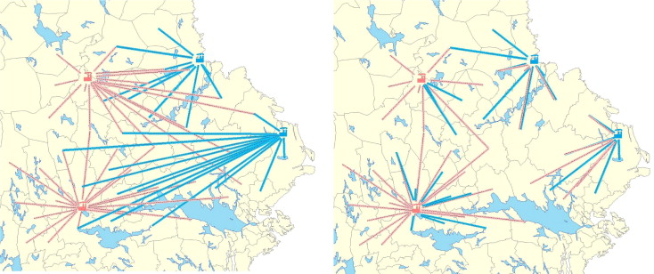
Figure 1: Two different companies (in red and blue) having different production-distribution centers that serve different customers located in a common region. The picture on the left shows the flows from the production-distribution centers if each company operates independently and that on the right shows what it could be if the two companies would join forces. The distance travelled is obviously smaller on the right. The main question here is: if the two company cooperate, how should they share the benefit associated with this reduction? Source: [10]

In the following we propose a general model for studying the corresponding problem and we introduce in particular a new family of cooperative games that we call production-distribution games. To the best of our knowledge, the corresponding models have not been studied so far, even though they are closely related to a classical model by Shapley and Shubik ([22], see Section 2). We believe that these models are well suited to address Open Problem 6 as we detail later. Also we believe that the underlying models would be useful to tackle similar questions that arise in the sector of urban distribution and beyond [5]. The originality of our model lies in the fact that the value/strength of a player does not only depend on the individual cost or benefit of the objects she owns (as is typically the case for combinatorial games e.g. flow games, matching games, shortest path games [7, 23, 12, 1]) but it also depends on her market shares: in particular a player can bring value to a coalition even if she has infinite production-distribution costs but “owns” some demand (i.e., market share) and vice-versa a player can bring value if she has low production-distribution costs but no demand.

There are different standard solution concepts in cooperative game theory when it comes to splitting (transferable) utility fairly among the different actors involved in a coalition. The most popular are the Core [11], the Shapley value [20] and the Nucleolus [18]. Our main goal in this study is to offer practitioners solutions that are sound conceptually but also attractive computationally (and thus possibly implementable). We mainly focus on the nucleolus which gained traction in the past years from this perspective as new polytime algorithms were developed (e.g. [1, 12]), building upon the linear programming (re)formulation of the different steps of the Maschler’s scheme [14], the main computational approach used to compute the nucleolus.

Könemann and Toth [13] introduced a general framework that allows to identify polytime solvability of the nucleolus when the maximum violation problem (separating over the core of the game with a maximally violated inequality) can be phrased as a (integral) dynamic program. The underlying algorithm is prohibitive computationally, however we believe that it should serve, first and foremost, as a guide to identify problems that can be tackled efficiently in principle (pretty much as the equivalence between separation and optimization in combinatorial optimization).

The main contribution of this paper is providing polynomial time algorithms to compute the nucleolus in a special case of these production-distribution games where the producers collaborate to serve a single market and they have infinite capacity (or at least a large enough capacity to accommodate all the demand of the corresponding market). We provide two algorithms: the former is a “standard” separation algorithm (see Section 4.1), the latter is an original and efficient primal-dual algorithm (see Section 4.2). Note that the corresponding problem fits the framework in [13] and it can thus be proven to be polytime solvable (see Section 4); however the primal-dual algorithm is much faster. We also show how to efficiently compute the Shapley value for the uncapacitated single market production-distribution game (see Section 5) with a rather standard and simple argument. Building on the fact that the uncapacitated multi market case can be written as the sum of uncapacitated single market production-distribution games, we can use additivity of the Shapley value to extend the solution to this setting (see Section 6). Although additivity does not hold for the nucleolus, we provide in addition, an alternative solution to the uncapacitated multi market case by summing up the different single market nucleolus: this solution is in the core and we believe that it is sound in practice.

Finally, the production-distribution games exhibit nice properties (e.g. non-emptyness of the core, polytime solvability of the nucleolus in interesting special cases) and challenging open mathematical problems (e.g. computational complexity of finding a point in the core in general and of computing the nucleolus and the Shapley value) that should hopefully trigger both the interest of practitioners and of academics.

2 The production-distribution game

We assume that a set $N=\{1,...,n\}$ of $n$ price-taker companies, producing a same commodity product, such as timber, are willing to cooperate to increase their profit. The most general model assumes that the commodity product is sold in a set $M=\{1,...,m\}$ of $m$ of different markets or countries. In each market $j\in M$, each unit of the commodity is sold at a common price $r_{j}$, and the cost bore by company $i\in N$ for producing and/or transporting (see Fig. 1) each unit of the commodity from its production centers to market $j$ is $c_{ij}$.

We also assume that each company $i\in N$ owns a part $d_{ij}\geq 0$ of the total demand $d_{j}$ in market $j\in M$, with $d_{j}:=\sum_{i\in N}d_{ij}$. Finally, we assume that there is an upper bound $q_{i}\geq 0$ on the production capacity of company $i$ (possibly $q_{i}=\infty$, i.e., there is no such bound) and that all players can serve their own demand, that is $q_{i}\geq\sum_{j\in M}d_{ij}$, for each $i\in N$.

If a subset $S\subseteq N$ of players collaborate, they achieve a total profit of $v(S)$ defined as follows:

$$v(S)=\max\sum_{i\in S}\sum_{j\in M}(r_{j}-c_{ij})y_{ij} s.t.$$ (1)

$$\sum_{i\in S}y_{ij}\leq\sum_{i\in S}d_{ij} \forall j\in M$$

$$\sum_{j\in M}y_{ij}\leq q_{i} \forall i\in S$$

$$y_{ij}\geq 0 \forall i\in S,j\in M$$

where $y_{ij}$ is the amount of commodity that company $i$ produces and distributes for market $j$. Note that we allow, in principle, not all demands to be served if it is not profitable, although each coalition has enough capacity since for each $i\in N$, $q_{i}\geq\sum_{j\in M}d_{ij}$. We now consider the cooperative game $(N,v)$ and we call it the production-distribution game. Note that the model naturally applies to the forestry setting if we assume that the players share information on a regular basis, say monthly, about their demand and costs (possibly through a third party that guarantees confidentiality of the corresponding data).

We are going to show that the production-distribution game is closely related to a classical model due to Shapley and Shubik (see the following). In order to do that, it is first convenient to make a few assumptions that, as we show in the following, can be taken without loss of generality for the production-distribution game. Namely, we will assume that $(i)$ $r_{j}\geq c_{ij}$, for any $i\in N$ and $j\in M$ and that $(ii)$ we may ask for equality in constraints $\sum_{i\in S}y_{ij}\leq\sum_{i\in S}d_{ij},\ \forall j\in M$. $(i)$ We assume that, $r_{j}\geq c_{ij}$, for any $i\in N$ and $j\in M$: indeed there is no reason to serve any demand on market $j$ from a player $i$ if $r_{j}<c_{ij}$, as we would be better off by not serving this demand. We can thus substitute any $c_{ij}$ such that $c_{ij}>r_{j}$ by redefining $c_{ij}=r_{j}$: if in an optimal solution to (1), $y_{ij}$ is not zero for such a situation, one should simply remember to set it to zero in a post-processing phase. Now observe that once we make the assumption that $r_{j}\geq c_{ij}$, for any $i\in N$ and $j\in M$, we may as well assume that $(ii)$ there is equality in constraints $\sum_{i\in S}y_{ij}\leq\sum_{i\in S}d_{ij},\ \forall j\in M$ as, if not, we could increase the value of some $y_{ij}$ since $\sum_{i\in S}\sum_{j\in M}d_{ij}\leq\sum_{i\in S}q_{i}$. Hence, we assume $(i)$ and $(ii)$ without loss of generality, and then we evaluate $v(S)$ as follows:

$$v(S)=\max\sum_{i\in S}\sum_{j\in M}(r_{j}-c_{ij})y_{ij} s.t.$$ (2)

$$\sum_{i\in S}y_{ij}=\sum_{i\in S}d_{ij} \forall j\in M$$

$$\sum_{j\in M}y_{ij}\leq q_{i} \forall i\in S$$

$$y_{ij}\geq 0 \forall i\in S,j\in M$$

We now recall the classical market game model, due to Shapley and Shubik [22]. The market game models an environment where there is a given, fixed quantity of $m$ continuous goods. Initially, these goods are distributed among $n$ players in an arbitrary way: each player $i\in N$ is endowed with an initial vector $d_{i}\in\mathbb{R}_{+}^{m}$. Also each player $i$ has a valuation function $f_{i}:\mathbb{R}_{+}^{m}\mapsto\mathbb{R}$ that takes as input any endowment vectors and outputs a utility for possessing these goods: $f_{i}$ is assumed to be continuous and concave. To increase their utility, players are free to trade goods. When the agents are forming a coalition, they are trying to allocate the goods such that the value of the coalition (i.e., the sum of the utility of each member of the coalition) is maximized. Namely, the value $v^{\prime}(S)$ of each coalition $S\subseteq N$ is given by:

$$v^{\prime}(S)=\max\{\sum_{i\in S}f_{i}(z_{i})\ |\ z_{i}\in\mathbb{R}_{+}^{m},\sum_{i\in S}z_{i}=\sum_{i\in S}d_{i}\}.$$

As we now show, the production-distribution game can be modeled as a market game. The main remark is the following: demands are traded among players in the production-distribution game as goods in the market game. So we may think of each market $j\in M$ as a different good; then each player $i\in N$ is endowed with an initial amount $d_{i}\in\mathbb{R}_{+}^{m}$ of goods. Also for each player $i\in N$, the valuation function $f_{i}(\cdot)$, which returns the profit of player $i$ when provided with endowment vector $z_{i}$, possibly different from $d_{i}$, is the following:

$$f_{i}(z_{i})=\max\sum_{j\in M}(r_{j}-c_{ij})y_{ij} s.t.$$ (3)

$$y_{ij}\leq z_{ij} \forall j\in M$$

$$\sum_{j\in M}y_{ij}\leq q_{i}$$

$$y_{ij}\geq 0 \forall j\in M$$

We are left with showing that $v^{\prime}(S)$ coincide with $v(S)$ as defined in (2). Observe that, through utility function $f_{i}$, player $i$ will optimize her personal profit given that she is given demands $z_{i}$ and has capacity $q_{i}$. In particular, if $z_{i}$ is such that $\sum_{j\in M}z_{ij}\leq q_{i}$, we can assume w.l.o.g. that she will serve all demands $z_{i}$ (remember that $r_{j}-c_{ij}\geq 0$). In this case, $f_{i}(z_{i})=\sum_{j\in M}(r_{j}-c_{ij})z_{ij}$. Also observe that if $\sum_{j\in M}z_{ij}>q_{i}$, the demand $\sum_{j\in M}z_{ij}-q_{i}$ is “lost” for player $i$ and all other players in the coalition. Hence in an optimal solution $z$ to $v^{\prime}(S)=\max\{\sum_{i\in S}f_{i}(z_{i})\ |\ z_{i}\in\mathbb{R}_{+}^{m},\sum_{i\in S}z_{i}=\sum_{i\in S}d_{i}\}$, we have w.l.o.g. $\sum_{j\in M}z_{ij}\leq q_{i}$ for each player $i\in S$: if not we can reassign the ‘lost’ demand of a player to other players in $S$ as in a feasible solution we have $\sum_{i\in S}z_{ij}=\sum_{i\in S}d_{ij}$ for all $j\in M$ and thus $\sum_{j\in M}\sum_{i\in S}z_{ij}=\sum_{j\in M}\sum_{i\in S}d_{ij}=\sum_{i\in S}\sum_{j\in M}d_{ij}\leq\sum_{i\in S}q_{i}$. It follows that $v^{\prime}(S)$ coincide with $v(S)$ as defined in (2).

We finally point out that, for each $S\subseteq N$, the constraint matrix of (2) is totally unimodular; therefore, if we restrict to demands and capacities that are integral, also the optimal solution to (2) is integral; then the standard assumption for the market game model that the commodity product is continuous holds without loss generality for the production-distribution game.

2.1 The core of the production-distribution game

The core $\mathcal{C}$ of a production-distribution game $(N,v)$ is the set of all imputations $x\in\mathbb{R}^{n}_{+}$ (redistribution of the global profit $v(N)$) that ensures that no coalition has an incentive to break the grand coalition $N$, that is, $\mathcal{C}$ is the set of $x$ such that:

$$x(N)=v(N)$$

$$x(S)\geq v(S) \forall S\subseteq N$$

The core of the market game is non-empty [22]. Then, since the production-distribution game can be modeled as a market game, then also the core of the production-distribution game is non-empty. However, we point out that the argument in [22] for proving non-emptyness of the core is not constructive (it uses the Bondareva-Shapley Theorem [3, 21]) and therefore it does not indeed provide a point in the core.

3 The nucleolus of the production-distribution game and the Maschler scheme

The nucleolus offers a desirable payoff-sharing solution in cooperative games, thanks to its attractive properties (see the following). In this section, we first recall its definition and then deal with the case of production-distribution games.

Let ${\cal N}_{p}=2^{N}\setminus\{N,\emptyset\}$. For each $x\in\mathbb{R}^{n}$ such that $x(N)=v(N)$ and for each $S\in{\cal N}_{p}$, we define the excess of coalition $S$ at $x$ as: $e_{S}(x)=x(S)-v(S)$. We also define the vector $e(x)\in\mathbb{R}^{2^{n}-2}$ of the excess of the different coalitions at $x$ as $e(x)=(e_{S}(x))_{S\in{\cal N}_{p}}$. Let $\vec{e}(x)$ be a permutation of the entries of $e(x)$ arranged in non-decreasing order. We say that $e(x)$ is leximin superior to $e(y)$ [$e(x)\succ e(y)$] if $\vec{e}(x)$ is lexicographically superior to $\vec{e}(y)$

Definition 1

: The (pre)nucleolus of a cooperative game $(N,v)$ is $nc(N,v):=\{x\in\mathbb{R}^{n}:x(N)=v(N)$ and $\not\exists y\in\mathbb{R}^{n}:y(N)=v(N),e(y)\succ e(x)\}$.

Note that the nucleolus is known to be a single point and moreover, it is in the core when the core is non-empty, as with production-distribution games. We are interested in polynomial time algorithms to compute the nucleolus. We are not aware of any such result for market games. It is known that the nucleolus can be computed in polynomial time for the class of convex games [8]. Unfortunately, the production-distribution game does not fit into the framework of convex games not even in the case of uncapacitated single market, as it is witnessed by the following example.

Example 1

Consider a problem with 3 producers and a single market with the following input: $r=2$, $c_{1}=1,c_{2}=1,c_{3}=2$, $d_{1}=d_{2}=d_{3}=1/3$. Consider the set $S=\{1,3\}$, $T=\{2,3\}$. We have $v(S)+v(T)=2/3+2/3=4/3>0+1=v(S\cap T)+v(S\cup T)$.

It is however known that the nucleolus can be computed by solving a sequence of at most $n$ linear programs: this is known as Maschler scheme [14]. Building upon this scheme, we will be able in the next section to provide polynomial time algorithms to find the nucleolus for the uncapacitated single-market production-distribution game. We therefore devote this section to recall this scheme.

The idea of the Maschler scheme is to start by making the worst possible excess as large as possible and then, given the constraints that it imposes on the problem, proceed by making the second worst excess as large as possible, etc. More formally, this can be formulated as follows. Given a polytope $P\subseteq\mathbb{R}^{n}_{+}$, we define $\mathcal{F}(P):=\{S\subseteq N,x(S)=y(S),\mbox{ for any }x,y\in P\}.$ First solve the following linear program:

$$\mbox{max }\epsilon$$

$$(P^{1})\ \ \ \ x(S)\geq v(S)+\epsilon \forall S\in{\cal N}_{p}$$

$$x(N)=v(N)$$

and let $\epsilon^{1}$ be the optimal value of ($P^{1}$) (for production-distribution games, $\epsilon^{1}\geq 0$, as the core is non-empty and the problem is bounded). Let $P^{1}(\epsilon^{1})$ be the polytope defined by the set of solutions $x\in\mathbb{R}^{n}_{+}$ such that $(x,\epsilon^{1})$ is an optimal solution to ($P^{1}$), $P^{1}(\epsilon^{1})$ is known as the leastcore. Note that the following holds:

$$P^{1}(\epsilon^{1})=\{x\in\mathbb{R}^{n}_{+}:x(S)\geq v(S)+\epsilon^{1},\forall S\in{\cal N}_{p};x(S)=c^{1}(S),\forall S\in\mathcal{F}(P^{1}(\epsilon^{1}))\},$$

for some function $c^{1}$. Observe also that in order to describe $\mathcal{F}(P^{1}(\epsilon^{1}))$ it is enough to keep track of a linear number of sets, say $S_{1},S_{2},...,S_{l}$, with $l\leq n$, whose characteristic vectors are linearly independent (we later simply say that the sets are linearly independent), as all other constraints of the form $x(S)=c^{1}(S)$ will then be implied by $x(S_{i})=c^{1}(S_{i})$ for $i=1,...,l$. Once we have found $P^{1}(\epsilon^{1})$, we can iterate, and solve for $k\geq 2$ the following linear program:

$$\mbox{max }\epsilon$$

$$(P^{k})\ \ \ \ x(S)\geq v(S)+\epsilon \forall S\in{\cal N}_{p}\setminus\mathcal{F}(P^{k-1}(\epsilon^{k-1}))$$

$$x\in P^{k-1}(\epsilon^{k-1}).$$

until the set of feasible solutions to ($P^{k}$) is made of a single point. Here $P^{k}(\epsilon^{k})$ is the polytope defined by the set of solutions $x^{k}\in\mathbb{R}^{n}_{+}$ such that $(x^{k},\epsilon^{k})$ is an optimal solution to ($P^{k}$): $P^{k}(\epsilon^{k})$ is well defined as, by induction, $P^{k}(\epsilon^{k})\subseteq P^{k-1}(\epsilon^{k-1})\ldots\subseteq P^{1}(\epsilon^{1})$, with each polytope bounded and non-empty. Note again that, through a similar discussion as above:

$$P^{k}(\epsilon^{k})=\{x\in\mathbb{R}^{n}_{+}:x(S)\geq v(S)+\epsilon^{k},\forall S\in{\cal N}_{p}\setminus\mathcal{F}(P^{k-1}(\epsilon^{k-1}));x(S)=c^{k}(S),\forall S\in\mathcal{F}(P^{k}(\epsilon^{k}))\},$$

for some functions $c^{1},...,c^{k}$ that satisfy $c^{k}(S)=c^{k-1}(S)$ for all $S\in\mathcal{F}(P^{k-1}(\epsilon^{k-1}))$ (note that $\mathcal{F}(P^{k-1}(\epsilon^{k-1}))\subseteq\mathcal{F}(P^{k}(\epsilon^{k}))$). Observe again that it is still enough to keep track of a linear number of (linearly independent) sets $S_{1},...,S_{k^{\prime}}$ in $\mathcal{F}(P^{k}(\epsilon^{k}))$. The Maschler scheme is known to converge in at most $n$ iterations as the dimension of $P^{k}(\epsilon^{k})$ decreases in each iteration.

3.1 A slightly revised Maschler scheme

Note that it is possible to slightly change the iterations of the Maschler scheme by simply setting to equality the sets corresponding to some constraints with positive dual values (and possibly other equalities implied by this choice) in an optimal basic solution to the linear programs above. From linear programming duality all the corresponding inequalities have to be satisfy to equality by all optimal solutions. This lead to a slight variation of the Maschler scheme where we impose to satisfy at equality only a subset of all equalities associated with the optimal face of each $(P^{k})$. The procedure would converge in a finite number of steps as in each step, there is at least one variable with positive dual value associated with a set $S$ such that $x(S)$ is not fixed yet (and will be fixed in this iteration), given the fact that the objective function only involves $\epsilon$. Hence if, in each iteration, we substitute $\mathcal{F}(P^{k-1}(\epsilon^{k-1}))$ by a certain subset $\mathcal{F}^{k}\subseteq\mathcal{F}(P^{k-1}(\epsilon^{k-1}))$, the revised scheme consists in solving for $k\geq 1$ (and until there is only one solution remaining):

$$\mbox{max }\epsilon$$

$$(M^{k})\ \ \ \ x(S)\geq v(S)+\epsilon\ \ \ \forall S\in{\cal N}_{p}\setminus\mathcal{F}^{k}$$ (4)

$$x(S)=c^{k}(S)\ \ \ \ \ \ \forall S\in\mathcal{F}^{k}$$

with $\mathcal{F}^{1}=\{N\}$, $c^{1}(N)=v(N)$ and, for $k\geq 2$, for some function $c^{k}(S)$ that satisfies $c^{k}(S)=c^{k-1}(S)$ for all $S\in\mathcal{F}^{k-1}$. Note that $\mathcal{F}^{k}\subset\mathcal{F}^{k+1}$ as, when moving from $(M^{k})$ to $(M^{k+1})$, we only fix additional inequalities to equalities: namely, we take some inequalities in $(M^{k})$ with positive dual value in the optimal solution to the dual, say $x(S)\geq v(S)+\epsilon$, fix $x(S)=v(S)+\epsilon^{k}$ ($\epsilon^{k}$ is the optimal value of $(M^{k})$), and suitably define $c^{k}(S)$ by possibly adding other equalities implied when considering in addition the system $x(S)=c^{k-1}(S)$ (for instance, if we fix $x(S)=v(S)+\epsilon^{k}$, then we may as well fix $x(N\setminus S)=v(N)-(v(S)+\epsilon^{k})$). We point out the following fact which will be often used:

Fact 1

An optimal solution $(x^{k},\epsilon^{k})$ to ($M^{k}$) is a feasible solution to ($M^{k+1}$).

4 The nucleolus for the uncapacitated single-market production-distribution game

We now deal with the production-distribution game for the case where there is a single market and there are no upper bounds on the production capacity of companies, i.e., $q_{i}=\infty$ for each $i\in N$. In this case, we may assume that the commodity product is sold at market price $r$ and the (per unit) production cost for company $i$ is $c_{i}$. We denote by $\alpha_{i}=r-c_{i}$ the (per unit) profit of company $i$ and we assume without loss of generality (see the discussion in Section 2) that $\alpha_{1}\geq\alpha_{2}\geq...\geq\alpha_{n}\geq 0$. Besides, we assume, without loss of generality, that the total demand is 1 and that each player $i$ owns a fraction $\lambda_{i}$ of this demand. Note that in this case, for a set $S$ such that $i\in S$ and $S\cap\{1,...,i-1\}=\emptyset$, $v(S)=\alpha_{i}\lambda(S)$.

We will provide polynomial two time algorithms to find the nucleolus for the uncapacitated single-market production-distribution game. The former relies on a “standard” separation algorithm (see Section 4.1); the latter is an original and efficient primal-dual algorithm (see Section 4.2). After the design of these algorithms, we became aware of the general framework from [13] to derive polynomial time algorithms for computing the nucleolus when the minimum excess coalition problem can be solved in polynomial time via an integral dynamic program. It is not difficult to see that the single-market problem without capacities fits this framework, as we quickly recap in the following. However, the separation algorithm from Section 4.1 is more direct that the one coming from using that framework. Even more interesting, the primal-dual algorithm from Section 4.2 is combinatorial (and much faster).

The framework of Könemann and Toth

Könemann and Toth [13] showed that the nucleolus can be computed via the Maschker scheme in polynomial time when the minimum excess coalition problem can be solved in polynomial time via an integral dynamic program. The minimum excess coalition problem is the following: given $x\in\mathbb{R}^{n}$, find $S\in\operatorname*{argmin}\{x(S)-v(S),S\subseteq N\}$.

In our setting, if we enumerate over the $n$ different possibilities for the minimum index $j$ in a solution set $S$ to the minimum excess coalition problem, then the problem $\operatorname*{argmin}\{x(S)-v(S),S\subseteq N\}$ decomposes into $n$ problems of the form $\operatorname*{argmin}\{x(S)-\alpha_{j}\cdot\lambda(S):S\subseteq\{j,...,n\}\mbox{ and }j\in S\}$. The latter problem is of the form $\operatorname*{argmin}\{\sum_{i\in S}y_{i}:S\subseteq\{j,...,n\}\mbox{ and }j\in S\}\}$, for $y_{i}=x_{i}-\alpha_{j}\cdot\lambda_{i}$. It can be modeled as a shortest path problem from vertex $j$ to vertex $n+1$ in the complete directed acyclic graph $G_{j}$ with $n-j+2$ vertices (one vertex for each element in $S$, numbered $j,...,n$, and one extra vertex, numbered $n+1$, representing a sink), induced by (topologically) ordering the vertices according to their numbering, and where the cost of an arc $(u,v)$ is simply $y_{u}$ (the nodes of the shortest path that are in $\{j,...,n\}$ will be the elements of $S$ to be considered).

Now observe that the disjunction over the different values of $j$ can be represented by a shortest path from a source node $s$ to a sink node $t$ in a larger directed acyclic graph obtained by taking the (disjoint) union of the directed acyclic graphs $G_{j}$, $j=1,...,n$ and adding a node $s$ with an arc (of zero cost) to the source node $j$ of $G_{j}$ and a node $t$ with an arc (of zero cost) from each sink node $n+1$ of $G_{j}$. The shortest path problem in a directed acyclic graph can be phrased as an integral dynamic program and thus polynomial time solvability is a consequence of [13].

4.1 Separation algorithm

In order to compute the nucleolus of the production-distribution game we again rely on the Maschler scheme. Following the discussion in Section 3, the scheme requires the solution, for each $k\geq 1$, of a linear program of this kind:

$$\mbox{max }\epsilon$$

$$(P^{k})\ \ \ \ x(S)\geq v(S)+\epsilon\ \ \ \forall S:S\not\in span\{S_{1},...,S_{k^{\prime}}\}$$ (5)

$$x(S)=c^{k}(S)\ \ \ \ \ \ \forall S:S\in span\{S_{1},...,S_{k^{\prime}}\}$$ (6)

for a given family of linearly independent sets $S_{1},...,S_{k^{\prime}}$.

We will now show how to separate any point from the polytope defined by (5)-(6) in polynomial time. We show later that, from the equivalence between separation and optimization, and because the above sequence is made of at most $n$ iterations, the nucleolus can be computed in polynomial time for the production-distribution game.

Let us introduce a couple of notations we will use in the following. For a set $S\subseteq E$ and $e\in E$, we denote by $S-e$ the set $S\setminus\{e\}$ and by $S+e$ the set $S\cup\{e\}$. A set $\{a,...,b\}$ with $b<a$ is the empty set (not the set $\{b,...,a\}$).

Lemma 1

There exists a polynomial time algorithm for separating over the polytope (5)-(6) for the production-distribution game.

Proof

Let $(x^{*},\epsilon^{*})$ be a point in $\mathbb{R}^{n+1}$ such that $x^{*}(N)=v(N)$ and $x^{*}(S)=c^{k}(S)$ for all $S\in\{S_{1},...,S_{k^{\prime}}\}$. We want to decide whether $x^{*}$ satisfies inequalities (5)-(6) and in case not, find a separating inequality.

The question reduces to testing whether there exists $S\subseteq\{1,...,n\}$, with $S\not\in span\{S_{1},...,S_{k^{\prime}}\}$ such that $x^{*}(S)<v(S)+\epsilon^{*}$. This is equivalent to checking for each $i=1,...,n$ and all $S$ s.t. $i\in S$, $S\cap\{1,...,i-1\}=\emptyset$ and $S\not\in span\{S_{1},...,S_{k^{\prime}}\}$ whether $x^{*}(S)\geq\lambda(S)\cdot\alpha_{i}+\epsilon^{*}$. Setting $y_{i}^{*}:=x^{*}(S)-\lambda(S)\cdot\alpha_{i}$, this is equivalent to testing whether $y_{i}^{*}(S)\geq\epsilon^{*}$ or equivalently whether $y_{i}^{*}(S-i)\geq\epsilon^{*}-y^{*}_{i}(i)$.

More abstractly, for each $i$ the problem is of the following form. Given $a_{1}\leq...\leq a_{p}$ and $b$ in $\mathbb{R}$, a set $M$ with $M\cap\{1,...,p\}=\emptyset$ and linearly independent sets $S_{1},...,S_{k}$ (over a ground set containing $M\cup\{1,...,p\}$) for some $0\leq k\leq p$, check whether $a(S)\geq b$ for all $S\subseteq\{1,...,p\}:S\cup M\not\in span\{S_{1},...,S_{k}\}$. From now on, we let $\mathcal{F}:=\{S\subseteq\{1,...,p\}:S\cup M\in span\{S_{1},...,S_{k}\}\}$. Also we say that the inequality associated with $S$ is violated if $a(S)<b$ (independently of whether $S$ is in $\mathcal{F}$ or not). In contrast, we talk of a separating inequality for a violated inequality associated with a set $S$ not in $\mathcal{F}$.

We define $\bar{j}:=\max\{j:a_{j}\leq 0\}$ (with the convention that $\bar{j}=0$ if $a_{1}>0$) and $\bar{S}:=\{1,...,\bar{j}\}$ and we assume also that $a(\bar{S})<b$ and $\bar{S}\in\mathcal{F}$ otherwise either there is no violated inequality (the one associated with $\bar{S}$ is the most (possibly) violated one as $\bar{S}$ minimizes $a(S)$ over all $S\subseteq\{1,...,p\}$) or the inequality associated with $\bar{S}$ is a separating inequality.

We define now

$$\underline{l}:=\min\{l\in\{1,...,\bar{j}\}:\bar{S}-l^{\prime}\in\mathcal{F}\mbox{ and }a(\bar{S}-l^{\prime})<b,\forall l^{\prime}:l\leq l^{\prime}\leq\bar{j}\}$$ (7)

$$\bar{l}:=\max\{l\in\{\bar{j}+1,...,n\}:\bar{S}+l^{\prime}\in\mathcal{F}\mbox{ and }a(\bar{S}+l^{\prime})<b,\forall l^{\prime}:l\geq l^{\prime}\geq\bar{j}+1\}$$ (8)

with the convention that $\underline{l}=0$ if $\bar{j}=0$, $\underline{l}=\bar{j}+1$ if no $l$ exists in $\{1,...,\bar{j}\}$ with the property required in (7), $\bar{l}=p+1$ if $\bar{j}=p$ and $\bar{l}=\bar{j}$ if no $l$ exists in $\{\bar{j}+1,...,p\}$ with the property required in (8). By definition we have $\bar{S}-(\underline{l}-1)\not\in\mathcal{F}$ or $a(\bar{S}-(\underline{l}-1))\geq b$ if $\underline{l}>1$ and $\bar{S}+(\bar{l}+1)\not\in\mathcal{F}$ or $a(\bar{S}+(\bar{l}+1))\geq b$ if $\bar{l}<p$.

If $\underline{l}>1$ and we have in addition that $\bar{S}-(\underline{l}-1)\not\in\mathcal{F}$ and $a(\bar{S}-(\underline{l}-1))<b$, the inequality associated with $\bar{S}-(\underline{l}-1)$ is a separating inequality. If $\bar{l}<p$ and we have in addition that $\bar{S}+(\bar{l}+1)\not\in\mathcal{F}$ and $a(\bar{S}+(\bar{l}+1))<b$, the inequality associated with $\bar{S}+(\bar{l}+1)$ is a separating inequality.

We claim that if we are not in one of the two situations above, there is no separating inequality. Observe first that, in such a case, any violated inequality must include all $l$ in $\{1,...,\underline{l}-1\}$ and must miss all $l$ in $\{\bar{l}+1,...,p\}$. Indeed, if $\underline{l}>1$, $a(\bar{S}-(\underline{l}-1))\geq b$. Similarly, if $\bar{l}<p$, $a(\bar{S}+(\bar{l}+1))\geq b$. But the most possibly violated inequality missing (at least) an element $l\in\{1,...,\underline{l}-1\}$ is the inequality associated with $\bar{S}-(\underline{l}-1))$ if $\underline{l}>1$ and the most possibly violated inequality including (at least) an element $l\in\{\bar{l}+1,...p\}$ is the inequality associated with $\bar{S}+(\bar{l}+1)$ if $\bar{l}<p$, which are both not violated.

So any possibly violated inequality is associated with a set of the form $\{1,...,\underline{l}-1\}\cup\tilde{S}$ for some $\tilde{S}\subseteq\{\underline{l},...,\bar{l}\}\cap\{1,...,p\}$. But $\{l\}\in span\{S_{1},...,S_{k}\}$ for all $l\in\{\underline{l},...,\bar{l}\}\cap\{1,...,p\}$ by construction (for all $l\geq 1:\underline{l}\leq l\leq\bar{j}$, $\bar{S}-l\in\mathcal{F}$ and $\bar{S}\in\mathcal{F}$, so $\bar{S}\setminus(\bar{S}-l)=(\bar{S}\cup M)\setminus((\bar{S}-l)\cup M)$ is in $span\{S_{1},...,S_{k}\}$ too, and for all $l\leq p:\bar{l}\geq l\geq\bar{j}+1$, $\bar{S}+l\in\mathcal{F}$ and $\bar{S}\in\mathcal{F}$, so $(\bar{S}+l)\setminus\bar{S}=((\bar{S}+l)\cup M)\setminus(\bar{S}\cup M)$ is in $span\{S_{1},...,S_{k}\}$ too), so it follows that $\bar{S}\setminus(\{\underline{l},...,\bar{j}\}\setminus\tilde{S})\cup(\tilde{S}\cap\{\bar{j}+1,...,\bar{l}\})=\{1,...,\underline{l}-1\}\cup\tilde{S}$ is in $\mathcal{F}$.

Corollary 1

The nucleolus can be found in polynomial time for the production-distribution game.

Proof

We can solve each linear program $(P^{k})$ in polynomial time from the equivalence between optimization and separation (note that at the first step, i.e., when $k=1$, the family $S_{1},...,S_{k^{\prime}}$ is made of the single set $N$). Besides, we can obtain in polynomial time a dual certificate associated with facets of (5)-(6) (see from Corollary 14.11.g in [19]). But any such dual certificate must contain at least one positive dual variable over the sets in (5) by definition of the dual (and because the objective function only contains $\epsilon$). It follows that we can find a set $S$ that is linearly independent of $S_{1},...,S_{k}^{\prime}$ and such that the inequality $x(S)\geq v(S)+\epsilon$ has to be satisfied at equality by all optimal solutions. And thus we can iterate and the scheme converges in at most $n$ iterations.

4.2 Combinatorial algorithm

We again rely on the Maschler scheme and in particular on the revised scheme discussed in Section 3.1. Namely we deal with the following linear program for $k\geq 1$ and until there is only one solution remaining:

$$\mbox{max }\epsilon$$

$$(M^{k})\ \ \ \ x(S)\geq v(S)+\epsilon\ \ \ \forall S\in{\cal N}_{p}\setminus\mathcal{F}^{k}$$ (9)

$$x(S)=c^{k}(S)\ \ \ \ \ \ \forall S\in\mathcal{F}^{k}$$

and we produce in polynomial time an optimal solution $(x^{k},\epsilon^{k})$ to each $(M^{k})$ starting from the optimal solution $(x^{k-1},\epsilon^{k-1})$ to $(M^{k-1})$, which is a feasible solution to $(M^{k})$, remember Fact 1; note that for $k=1$, the solution of $(M_{1})$ starts with the feasible solution $(x^{0},\epsilon^{0})$, where $x^{0}(j)=\lambda_{j}\cdot\alpha_{1}$ and $\epsilon^{0}=0$.

In particular, for each $k\geq 1$ the family $\mathcal{F}^{k}$ will hold a particular structure:

Property 1

$\mathcal{F}^{k}$ corresponds to all subsets of $F^{k}$ and their complement for a set $F^{k}\subseteq N$ such that $1\notin F^{k}$. Namely, $\mathcal{F}^{k}=\{F\in 2^{N}:$ either $F\subseteq F^{k}$ or $N\setminus F^{k}\subseteq F\}$.

We initially set $F^{1}=\emptyset$, and therefore $\mathcal{F}^{1}=\{N,\emptyset\}$. And we will guarantee a polynomial number of step in our revised scheme by ensuring that, at each iteration, $F^{k}$ is a strict superset of $F^{k-1}$: that will be done by exploiting for each problem $(M^{k})$ an optimal dual certificate. The scheme will then converge in at most $n-1$ iterations, as eventually $F^{k}=N\setminus 1$ and therefore $\mathcal{F}^{k}=2^{N}$: in this case, if $(x^{k-1},\epsilon^{k-1})$ is the optimal solution to ($M^{k-1}$), then $x^{k-1}$ is the nucleolus.

At each iteration $k$, we will solve program $(M^{k})$ by a suitable primal-dual algorithm, that we describe in the following.

Solving $(M^{k})$ by a primal-dual algorithm

First note that the problem ($M^{k}$) is actually the dual ($D^{k})$ of problem $(P^{k})$ below:

($P^{k}$) $\begin{array}[]{ll}\min&-\sum_{S\in\mathcal{F}^{k}}c^{k}(S)y_{S}-\sum_{S\notin\mathcal{F}^{k}}v(S)y_{S}\\ &Ay=0\\ &\sum_{S\not\in\mathcal{F}^{k}}y_{S}=1\\ &y_{S}\geq 0,\forall S\not\in\mathcal{F}^{k}\\ \end{array}$

($D^{k}$) $\begin{array}[]{ll}\max&\epsilon\\ &xA_{S}\geq v(S)+\epsilon,\forall S\not\in\mathcal{F}^{k}\\ &xA_{S}=c^{k}(S),\forall S\in\mathcal{F}^{k}\end{array}$

where $A$ is a matrix whose columns are the characteristic vectors of the sets $S\in{\cal N}_{p}$. We will then solve each program $(D^{k})\equiv(M^{k})$ by using the primal-dual algorithm applied to $(P^{k})$ (note that we will never need to know explicitly the values $c^{k}(S)$).

The primal-dual algorithm starts from the feasible dual solution $(x^{k-1},\epsilon^{k-1})$ to $(D^{k})$, see the discussion above. When $k=1$ we rely on the solution $(x^{0},\epsilon^{0})$, with $x^{0}(j)=\lambda_{j}\cdot\alpha_{1}$ and $\epsilon^{0}=0$. The current solution will be then updated through the iterative solution of a pair of auxiliary programs: the restricted primal ($RP$) and the dual of the restricted primal ($DRP$). Before providing these programs, we point out that throughout each iteration of the primal-dual algorithm we will assume that the current solution $(x,\epsilon)$ to $D^{k}$ will satisfy a suitable property:

Property 2

For each $i\not\in F^{k},i\neq 1$, $x(N\setminus i)=v(N\setminus i)+\epsilon$.

We point out that when $k=1$ Property 2 holds with respect to $(x^{0},\epsilon^{0})$ and $F^{1}=\emptyset$. We will show that, for a fixed $k$, Property 2 is then preserved over the iterations of the primal-dual algorithm: this way we will prove by induction that the property holds also with respect to the first solution to $(D^{k+1})\equiv(M^{k+1})$ as, once again, the optimal solution $(x^{k},\epsilon^{k})$ to $(D^{k})$ is the starting (feasible) solution to $(D^{k+1})$, and $F^{k+1}$ will be always a strict superset of $F^{k}$.

Also note that, as $1\notin F^{k}$ by Property 1, if $i\neq 1$ is not in $F^{k}$, then $N\setminus i\notin\mathcal{F}^{k}$. Through Property 2, we assume that even if the set $N\setminus i\notin\mathcal{F}^{k}$, the corresponding constraint in ($D^{k}$) is tight.

In the following, for shortness, we let $P:=P^{k},D:=D^{k},\mathcal{F}:=\mathcal{F}^{k}$, $F:=F^{k}$. Suppose therefore that we are given a feasible solution $(x,\epsilon)$ to $D$ with $N\setminus 1\not\subseteq F$ (else $x$ is the nucleolus, see above) that satisfies Property 2. As we want to apply the primal-dual algorithm (to solve $P$), we want to check optimality of $(x,\epsilon)$ using complementary slackness. It means: does there exist $y$ feasible solution to $P$ with $y_{S}=0$ whenever $S\not\in\mathcal{F}$ and $xA_{S}>v(S)+\epsilon$? The answer is “yes” if and only if the optimal solution to the restricted primal $RP$ below has value 0 (we let ($DRP$) be the dual of ($RP$)):

($RP$) $\begin{array}[]{ll}\min&\delta\\ &Ay=0\\ &\sum_{S\not\in\mathcal{F}}y_{S}+\delta=1\\ &y_{S}\geq 0,\forall S\not\in\mathcal{F}\\ &y_{S}=0,\forall S\not\in\mathcal{F}:xA_{S}>v(S)+\epsilon\\ &\delta\geq 0\\ \end{array}$

($DRP$) $\begin{array}[]{ll}\max&\tilde{\epsilon}\\ &\tilde{x}A_{S}\geq\tilde{\epsilon},\forall S\not\in\mathcal{F}:xA_{S}=v(S)+\epsilon\\ &\tilde{x}A_{S}=0,\forall S\in\mathcal{F}\\ &\tilde{\epsilon}\leq 1\end{array}$

Observe first that ($RP$) has a (optimal) solution of value 0 if and only if there is a feasible solution to the following system:

(I)	$\begin{array}[]{l}Ay=0\\ \sum_{S\not\in\mathcal{F}}y_{S}>0\\ y_{S}\geq 0,\forall S\not\in\mathcal{F}\\ y_{S}=0,\forall S\not\in\mathcal{F}:xA_{S}>v(S)+\epsilon\\ \end{array}$

as in this case we can scale $y$ to guarantee $\sum_{S\not\in\mathcal{F}}y_{S}=1$. Moreover, it follows that if ($RP$) does not have value $0$ then it has value $1$, as $y=0,\delta=1$ is a solution to ($RP$) (and if there is a solution ($RP$) with $1>\delta>0$, then we have a solution of value 0 to (I) and thus a solution to ($RP$), as we just observed).

Claim

Let $(x,\epsilon)$ be a feasible solution to $D$ with $N\setminus 1\not\subseteq F$. Then:

• if there exists $\bar{S}$: $\bar{S}\not\in\mathcal{F}$, $xA_{\bar{S}}=v({\bar{S}})+\epsilon$ and $1\not\in\bar{S}$, then $RP$ has value $0$;

• if vice versa each $\bar{S}$: $\bar{S}\not\in\mathcal{F}$, $xA_{\bar{S}}=v({\bar{S}})+\epsilon$ is such that $1\in\bar{S}$, then $RP$ has value $1$

Proof

Observe that, since $N\setminus 1\not\subseteq F$, it follows that there exist $i\neq 1:i\notin F$.

$(i)$. It is enough to prove that in this case there exists then a solution $y$ that satisfies (I). Note that $A_{\bar{S}}+\sum_{i\in\bar{S}}A_{N\setminus i}=|\bar{S}|A_{N}$. Hence setting $y_{\bar{S}}=1$, $y_{N\setminus i}=1$ for all $i\in\bar{S}$ and $y_{N}=-|\bar{S}|$, we have $Ay=0$. We now show that $y$ satisfies the other constraints in (I). First, $y$ satisfies constraints $y_{S}\geq 0,\forall S\not\in\mathcal{F}$, as $N\in\mathcal{F}$. Then $y$ satisfies constraints $y_{S}=0,\forall S\not\in\mathcal{F}:xA_{S}>v(S)+\epsilon$ by construction and Property 2. Finally we have $\sum_{S\not\in\mathcal{F}}y_{S}>0$ by construction (note again that $N\in\mathcal{F}$).

$(ii)$. Consider the solution to $DRP$ with $\tilde{\epsilon}=1$ and $\tilde{x}$ such that: $\tilde{x}(1)=n-1-|F|$; $\tilde{x}(i)=-1$ for all $i\not\in F,i\neq 1$; $\tilde{x}(i)=0$ for all $i\in F$. It has value $1$ so let us check that it is feasible. For all $S\in\mathcal{F}$, either $S\subseteq F$ and in this case $\tilde{x}A_{S}=0$ ; or $S$ is the complement of a subset of $F$. In the latter case, $1\in S$ (by Property 1) and thus $\tilde{x}A_{S}=n-1-|F|-(|S\setminus F|-1)=|N\setminus F|-1-(|S\setminus F|-1)=0$. Now consider any set $S$ such that $S\not\in\mathcal{F}$ and $xA_{S}=v(S)+\epsilon$: by hypothesis $1\in S$. In this case, $\tilde{x}A_{S}=n-1-|F|-(|S\setminus F|-1)$. As $S\not\in\mathcal{F}$, it follows that $N\setminus(F\cup S)\neq\emptyset$: otherwise $S$ is the complement of $F\setminus S$ and by hypothesis it is in $\mathcal{F}$. Then $n-1-|F|-(|S\setminus F|-1)=|N\setminus F|-1-(|S\setminus F|-1)=|N\setminus F|-|S\setminus F|\geq 1$. Hence $(\tilde{x},\tilde{\epsilon})$ is a feasible solution to $DRP$ with value 1.

Hence, in order to check optimality of the current solution $(x,\epsilon)$, we only need to check whether there exists $\bar{S}$: $\bar{S}\not\in\mathcal{F}:xA_{\bar{S}}=v({\bar{S}})+\epsilon$ with $1\not\in\bar{S}$. If there exists such a $\bar{S}$, $(x,\epsilon)$ is an optimal solution to the current iteration of the Maschler scheme. We then replace $F$ by $\bar{S}\cup F$: note there must exist an element in $\bar{S}\setminus F$ otherwise $\bar{S}$ is a subset of $F$, and hence in $\mathcal{F}$, a contradiction.

If vice versa, each $\bar{S}$: $\bar{S}\not\in\mathcal{F}$, $xA_{\bar{S}}=v({\bar{S}})+\epsilon$ is such that $1\in\bar{S}$ then from the proof of Claim 4 (i), $(\tilde{x},{\tilde{\epsilon}})$ – with ${\tilde{\epsilon}}=1$, $\tilde{x}(1)=n-1-|F|$; $\tilde{x}(i)=-1$ for all $i\not\in F,i\neq 1$; $\tilde{x}(i)=0$ for all $i\in F$ – is an optimal solution to $DRP$. According to the primal-dual algorithm, we use $(\tilde{x},\tilde{\epsilon})$ to update $(x,\epsilon)$. Namely, we look for the maximum increase in the direction of $(\tilde{x},\tilde{\epsilon})$ by finding the maximum $\lambda\geq 0$ such that $(x,\epsilon)+\lambda(\tilde{x},\tilde{\epsilon})$ remains feasible for $D$. Observe that: if $S\in\mathcal{F}$, then $\tilde{x}A_{S}=0$; if $S\not\in\mathcal{F}$ and $1\in S$, then $\tilde{x}A_{S}\geq\tilde{\epsilon}$. Hence, the restriction can only come from a set $S\not\in\mathcal{F}$ with $1\not\in S$: in this case, $xA_{S}>v(S)+\epsilon$ (otherwise the value of $RP$ would be 0) and $\tilde{x}A_{S}<\tilde{\epsilon}$ (this holds for all $S$ not taking $1$). Thus $\lambda$ can be defined as follows:

$\lambda=\min_{S\not\in\mathcal{F},1\not\in S}\frac{xA_{S}-v(S)-\epsilon}{\tilde{\epsilon}-\tilde{x}A_{S}}=\frac{xA_{S}-v(S)-\epsilon}{1+|S\setminus F|}$

Note that $\lambda>0$ as otherwise $RP$ would have value $0$. Let $\bar{S}$ be the argmin in the previous formula and let $(x,\epsilon)=(x,\epsilon)+\lambda(\tilde{x},\tilde{\epsilon})$. Obviously, for this new $(x,\epsilon)$, $xA_{\bar{S}}=v({\bar{S}})+\epsilon$ and by Claim 4, $RP$ has now value zero. We have therefore:

Lemma 2

The primal-dual algorithm converges in at most one iteration.

The only thing we need to prove now is that we keep Property 2 when the primal-dual iterates. Let $i\neq 1$, $i\notin F$. We have $xA_{N\setminus i}=v({N\setminus i})+\epsilon$ before the update by induction and $\tilde{x}A_{N\setminus i}=\tilde{\epsilon}$ (by construction), and thus we still have $xA_{N\setminus i}=v({N\setminus i})+\epsilon$ after the iteration.

As we already observe, we increase the size of $F$ in each iteration of the Maschler scheme so we converge in at most $n-1$ iterations. In order to prove polynomiality we thus only need to prove that computing $\lambda$, and actually whether $RP$ has value 0 or not, can be done in polytime. Note that we can solve the question of $RP$ having value $0$ or not first simultaneously to the computation of $\lambda$, as $\lambda=0$ if and only if $RP$ has value zero.

The computation of $\lambda$ is easy in our case. We will solve the problem by enumerating over all choices for $i\neq 1$ and over the possible values for $t:=|S\setminus F|$ (from $1$ to at most $n-1-|F|)$. For a fixed $i$ and $t$, we solve a problem of the form $\min_{S\in\mathcal{S}_{i}:S\notin\mathcal{F},|S\setminus F|=t}\frac{w(S)-\epsilon}{1+t}$ (hence we have to solve $O(n^{2})$ problems), which is equivalent to $\min_{S\in\mathcal{S}_{i}:S\notin\mathcal{F},|S\setminus F|=t}w(S)$ (as, $t$ and $\epsilon$ are fixed) and then to $\min_{S\in\mathcal{S}_{i}:S\not\subseteq F,|S\setminus F|=t}w(S)$ (for $i\neq 1$, we have that for all $S\in\mathcal{S}_{i}$, $1\notin S$, so $S$ cannot be the complement of a subset of $F$ when $S\not\subseteq F$). The solution is trivial: we take $i$ and all elements $j$ that are in $F\cap\{i+1,\ldots,n\}$ such that $w_{j}<0$ and we add either the smallest (with respect to the weight $w$) $t$ or $t-1$ elements (depending whether $i\in F$ or not) in $(N\setminus F)\cap\{i+1,\ldots,n\}$. The complexity of the algorithm is thus $O(n\cdot(n\log(n)+n^{2}\cdot n))=O(n^{4})$ (this could certainly be improved).

5 Shapley values for the uncapacitated single-market production-distribution game

Besides the nucleolus also the Shapley value [20] offers a desirable payoff-sharing solution in cooperative games, thanks to the property of being the unique cost sharing mechanism that satisfies the following axioms: efficiency; symmetry; linearity; null player property. The Shapley value $S_{i}(v)$ for player $i\in N$ in a cooperative game $(N,v)$ is equal to:

$$S_{i}(v)=\sum_{T\subseteq N:i\in T}\frac{(|T|-1)!(n-|T|)!}{n!}(v(T)-v(T\setminus\{i\}))=\sum_{T\subseteq N:i\in T}\beta_{|T|}\cdot(v(T)-v(T\setminus\{i\})),$$

where we let $\beta_{|T|}:=\frac{(|T|-1)!(n-|T|)!}{n!}$. If we now deal with the uncapacitated single market production-distribution game, and rely on the assumptions and definitions from Section 4 (see the first paragraph), it is straightforward to see that:

$$v(T)-v(T\setminus\{i\})=\left\{\begin{array}[]{ll}\lambda_{i}\cdot\alpha_{h}&\mbox{\ \ if\ }T\in{\cal S}_{h},h<i\\ &\\ \lambda(T\setminus i)\cdot(\alpha_{i}-\alpha_{h})+\lambda_{i}\cdot\alpha_{i}&\mbox{\ \ if\ }T=\{i\}\cup S,S\in{\cal S}_{h},h>i\\ &\\ \lambda_{i}\cdot\alpha_{i}&\mbox{\ \ if\ }T=\{i\}\end{array}\right.$$

where, for each $i=1,...,n$, ${\cal S}_{i}=\{S\subseteq N:S\cap\{1,2,\ldots,i\}=\{i\}\}$. It is now pretty straightforward to compute the Shapley value efficiently, it is simply a matter of computing appropriately the number of set $T\subseteq N:i\in T$ that fall into these three cases. Then a rather tedious calculus shows that:

$$S_{i}(v)=\lambda_{i}\sum_{h\in\{1,..,i-1\}}\ \alpha_{h}\sum_{l=0..n-h-1}{n-h-1\choose l}\beta_{l+2}\ +\ \alpha_{i}\frac{\lambda_{i}}{n}\ +\sum_{h\in\{i+1,..,n\}}\alpha_{i}\lambda_{i}\sum_{l=0..n-h}{n-h\choose l}\cdot\beta_{l+2}\ +$$

$$+\sum_{h\in\{i+1,..,n\}}(\alpha_{h}-\alpha_{i})(\lambda_{h}\ \sum_{l=0..n-h}{n-h\choose l}\beta_{l+2}\ +\ \sum_{j\in\{h+1,..n\}}\lambda_{j}\ \sum_{l=0..n-h-1}{n-h-1\choose l}\beta_{l+3})$$ (10)

and therefore the Shapley value can be computed in polynomial time. We recall that however in general the Shapley value needs not be in the core.

6 The uncapacitated multi market production-distribution game

In this section, we give up with the hypothesis of a single market and we consider a set $M$ of markets. However, we still assume that there is no upper bound on the production capacity of each company $i\in N$, i.e., $q_{i}=\infty$. We learned from Section 2.1, via a nonconstructive argument, that the core of the game $(N,v)$ is non-empty; however, as we show in the following, in this case one may easily exhibit a point in the core. First, let $\alpha_{ij}=r_{j}-c_{ij}$ (recall that we may assume without loss of generality that $\alpha_{ij}\geq 0$). It is easy to see that in this uncapacitated setting:

$$v(S)=\sum_{j\in M}\max_{i\in S}\alpha_{ij}\cdot\sum_{i\in S}d_{ij}.$$

This takes us to define a (sub)game $(N,v_{j})$ for each market $j\in M$. For a fixed $j\in M$, we consider the single market game with value function, $v_{j}(S):=\max_{i\in S}\alpha_{ij}\cdot d_{j}(S)$ (with $d_{j}(S):=\sum_{i\in S}d_{ij}$), for each $S\subseteq N$. Let $\alpha^{*}_{j}:=\max_{i\in N}\alpha_{ij}$. Then it is easy to check that the imputation $x_{i}=\alpha^{*}_{j}\cdot d_{ij}$, for all $i=1,...,n$, is in the core of the game $(N,v_{j})$. Now observe that $(N,v)=(N,\sum_{j\in M}v_{j})$, as for each $S\subseteq N$, $v(S)=\sum_{j\in M}v_{j}(S)$ and thus the imputation $x_{i}=\sum_{j\in M}\alpha^{*}_{j}\cdot d_{ij}$, for all $i=1,...,n$, is in the core of the game $(N,v)$. The fact that $(N,v)=(N,\sum_{j\in M}v_{j})$ combined with linearity of the Shapley shows that (we simply need to sum the values $S_{i}(v_{j})$ that can be computed from (10)) :

Corollary 2

The Shapley value can be found in polynomial time for the uncapacited multi market production-distribution game.

It is tempting to use the fact that $(N,v)=(N,\sum_{j\in M}v_{j})$ also to decompose the computation of the nucleolus. Unfortunately, in contrast with the Shapley value, the nucleolus is not additive in general and not even in this family of games, as illustrated by the following example.

Example 2

Consider a problem with 3 producers and 3 markets. The demand matrix $d:=(d_{ij})_{1\leq i,j\leq 3}$ and the profit matrix $\alpha:=(\alpha_{ij})_{1\leq i,j\leq 3}$, are given below:

$d=\left[\begin{array}[]{ccc}1&0&1\\ 0&1&1\\ 1&1&0\\ \end{array}\right]$ , $\alpha=\left[\begin{array}[]{ccc}1&1&1\\ 1&0&0\\ 0&0&1\\ \end{array}\right]$

Computation shows that the nucleolus of the associated production-distribution game is $x_{1}=10/3,x_{2}=4/3,x_{3}=4/3$. In contrast, the sum of the nucleolus associated with the 3 production-distribution games restricted to each market is $x_{1}=3,x_{2}=1.5,x_{3}=1.5$.

We believe that, although the solution provided by the sum of the nucleolus of the single-market subproblems does not coincide with the nucleolus in general, it is still as a sensible solution in practice since the solution to the single-market case can be computed quickly using the combinatorial algorithm presented in Section 4.2 and it seems reasonable to argue on each market separately. Besides, the corresponding solution is in the core of $(N,v)$ as, the core of each subgame $(N,v_{j})$ is non-empty, the nucleolus is in the core (for such non-empty games), and the sum of solutions in the core of $(N,v_{j})$ is obviously in the core of $(N,\sum_{j\in M}v_{j})=(N,v)$. Once again this is not always the case with the Shapley value.

Finally, the production-distribution games exhibit nice properties, such as the non-emptyness of the core, and the polytime solvability of the nucleolus and the Shapley values in interesting special cases. However there are still challenging open mathematical problems for general production-distribution games: Can we find a point in the core? Can we find the nucleolus or the Shapley values efficiently? We leave the corresponding questions for further investigations.

References

- [1] Baïou, M., Barahona, F.: An algorithm to compute the nucleolus of shortest path games. Algorithmica 81(8), 3099–3113 (2019). https://doi.org/10.1007/s00453-019-00574-9, https://doi.org/10.1007/s00453-019-00574-9
- [2] Basso, F., D’Amours, S., Rönnqvist, M., Weintraub, A.: A survey on obstacles and difficulties of practical implementation of horizontal collaboration in logistics. International Transactions in Operational Research 26(3), 775–793 (2019)
- [3] Bondareva, O.N.: Some applications of linear programming methods to the theory of cooperative games. Problemy kibernetiki 10(119), 139 (1963)
- [4] Chauhan, C., Kaur, P., Arrawatia, R., Ractham, P., Dhir, A.: Supply chain collaboration and sustainable development goals (sdgs). teamwork makes achieving sdgs dream work. Journal of Business Research 147, 290–307 (2022). https://doi.org/https://doi.org/10.1016/j.jbusres.2022.03.044, https://www.sciencedirect.com/science/article/pii/S0148296322002818
- [5] Cleophas, C., Cottrill, C., Ehmke, J.F., Tierney, K.: Collaborative urban transportation: Recent advances in theory and practice. European Journal of Operational Research 273(3), 801–816 (2019)
- [6] Cruijssen, F.C.A.M., et al.: Horizontal cooperation in transport and logistics. CentER, Tilburg University Tilburg (2006)
- [7] Deng, X., Fang, Q., Sun, X.: Finding nucleolus of flow game. Journal of combinatorial optimization 18(1), 64–86 (2009)
- [8] Faigle, U., Kern, W., Kuipers, J.: On the computation of the nucleolus of a cooperative game. International Journal of Game Theory 30(1), 79–98 (2001)
- [9] Flisberg, P., Frisk, M., Rönnqvist, M., Guajardo, M.: Potential savings and cost allocations for forest fuel transportation in Sweden: A country-wide study. Energy 85(C), 353–365 (2015)
- [10] Frisk, M., Göthe-Lundgren, M., Jörnsten, K., Rönnqvist, M.: Cost allocation in collaborative forest transportation. European Journal of Operational Research 205(2), 448–458 (2010). https://doi.org/https://doi.org/10.1016/j.ejor.2010.01.015, https://www.sciencedirect.com/science/article/pii/S0377221710000238
- [11] Gillies, D.B.: Solutions to general non-zero-sum games. Contributions to the Theory of Games 4, 47–85 (1959)
- [12] Könemann, J., Pashkovich, K., Toth, J.: Computing the nucleolus of weighted cooperative matching games in polynomial time. Mathematical Programming 183(1), 555–581 (2020)
- [13] Könemann, J., Toth, J.: A general framework for computing the nucleolus via dynamic programming. In: International Symposium on Algorithmic Game Theory. pp. 307–321. Springer (2020)
- [14] Maschler, M., Peleg, B., Shapley, L.S.: Geometric properties of the kernel, nucleolus, and related solution concepts. Mathematics of operations research 4(4), 303–338 (1979)
- [15] Pan, S., Ballot, E., Huang, G.Q., Montreuil, B.: Physical internet and interconnected logistics services: research and applications. International Journal of Production Research 55(9), 2603–2609 (2017). https://doi.org/10.1080/00207543.2017.1302620, https://doi.org/10.1080/00207543.2017.1302620
- [16] Pan, S., Trentesaux, D., Ballot, E., Huang, G.Q.: Horizontal collaborative transport: survey of solutions and practical implementation issues. International Journal of Production Research 57(15-16), 5340–5361 (2019). https://doi.org/10.1080/00207543.2019.1574040, https://doi.org/10.1080/00207543.2019.1574040
- [17] Rönnqvist, M., D’Amours, S., Weintraub, A., Jofre, A., Gunn, E., Haight, R.G., Martell, D., Murray, A.T., Romero, C.: Operations research challenges in forestry: 33 open problems. Annals of Operations Research 232(1), 11–40 (2015)
- [18] Schmeidler, D.: The nucleolus of a characteristic function game. SIAM Journal on applied mathematics 17(6), 1163–1170 (1969)
- [19] Schrijver, A.: Theory of linear and integer programming. John Wiley & Sons (1998)
- [20] Shapley: A value for n-person games. In: Kuhn, H. and Tucker, A., Eds., Contributions to the Theory of Games II. pp. 307–317. Princeton University Press (1953)
- [21] Shapley, L.S.: On balanced sets and cores. Tech. rep., Rand. Corp. Santa Monica Calif. (1965)
- [22] Shapley, L.S., Shubik, M.: On market games. Journal of Economic Theory 1(1), 9–25 (1969)
- [23] Shapley, L.S., Shubik, M.: The assignment game i: The core. International Journal of game theory 1(1), 111–130 (1971)