Efficient low temperature simulations for fermionic reservoirs with the hierarchical equations of motion method: Application to the Anderson impurity model

Abstract

The hierarchical equations of motion (HEOM) approach is an accurate method to simulate open system quantum dynamics, which allows for systematic convergence to numerically exact results. To represent effects of the bath, the reservoir correlation functions are usually decomposed into summation of multiple exponential terms in the HEOM method. Since the reservoir correlation functions become highly non-Markovian at low temperatures or when the bath has complex band structures, a present challenge is to obtain accurate exponential decompositions that allow efficient simulation with the HEOM. In this work, we employ the barycentric representation to approximate the Fermi function and hybridization functions in the frequency domain. The new method, by approximating these functions with optimized rational decomposition, greatly reduces the number of basis functions in decomposing the reservoir correlation functions, which further allows the HEOM method to be applied to ultra-low temperature and general band structures. We demonstrate the efficiency, accuracy, and long-time stability of the new decomposition scheme by applying it to the Anderson impurity model (AIM) in the low temperature regime with the Lorentzian and tight-binding hybridization functions.

I Introduction

A paradigmatic setting in solid state physics is related to a quantum system coupled to a continuum of electronic states, where a typical example is the charge transport in single-molecule junctions or through quantum dots Galperin et al. (2008); Zimbovskaya (2013); Ratner (2013); Xiang et al. (2016); Thoss and Evers (2018). Such systems usually consist of a molecule or quantum dot attached to two metal leads, forming an open quantum system where the molecule can exchange electrons and energy with the leads. Owing to the advances in experimental techniques Chen et al. (1999); Park et al. (2000, 2002); Xu and Tao (2003); Qiu et al. (2004), it is now possible to measure a variety of transport properties. The experimental observations, including Coulomb blockade Park et al. (2002), spin blockade Heersche et al. (2006), Kondo effect Liang et al. (2002); Parks et al. (2010), negative differential resistance Osorio et al. (2010); Chen et al. (1999); Gaudioso et al. (2000); Xu and Dubi (2015), switching Blum et al. (2005); Choi et al. (2006), and hysteresis Ballmann et al. (2012), have shown the potential of molecular junctions in the field of molecular electronics and stimulated the development of transport theory and simulation techniques.

Different methods are now available to solve the transport problem in molecular junctions and likewise for arrays of quantum dots. Approximate methods such as the quantum master equations (QMEs) Mitra et al. (2004); Donarini et al. (2006); Timm (2008); Leijnse and Wegewijs (2008); Esposito and Galperin (2009); Härtle and Thoss (2011); Levy et al. (2019), although being able to provide many useful physical insights, introduce significant approximations and are often limited to certain parameter regimes. For example, in a previous study, we have shown that QMEs based on perturbation theory fail in the strong coupling regime Dan et al. (2022). Many numerically exact methods have also been developed, which include the numerical renormalization group (NRG) Anders and Schiller (2005, 2006); Bulla et al. (2008); Nghiem and Costi (2018); de Souza Melo et al. (2019), density-matrix renormalization group (DMRG) Schollwöck (2005); Heidrich-Meisner et al. (2009); He and Millis (2019); Kohn and Santoro (2021), and multilayer multi-configuration time-dependent Hartree (ML-MCTDH) in the second quantization representation (SQR) Wang and Thoss (2009); Wang et al. (2011); Wang and Thoss (2018). These methods usually require discretization of the lead hybridization functions, such that special treatments are needed to avoid discretization artifacts at long simulation times Nishimoto and Jeckelmann (2004); Žitko and Pruschke (2009); Wang and Thoss (2018).

Other approaches utilize the non-interacting nature of the leads and do not require discretization. These include the path integral (PI) Weiss et al. (2008); Segal et al. (2010); Weiss et al. (2013), continuous-time quantum Monte-Carlo (CT-QMC) Mühlbacher and Rabani (2008); Werner et al. (2009); Schiró and Fabrizio (2009); Gull et al. (2011); Antipov et al. (2016); Krivenko et al. (2019), Inchworm Monte Carlo Cohen et al. (2015); Antipov et al. (2017), and the hierarchical equations of motion (HEOM) approach Jin et al. (2008); Li et al. (2012); Härtle et al. (2013, 2015); Shi et al. (2018); Erpenbeck et al. (2019); Zhang et al. (2020); Dan et al. (2022).

In this work, we focus on the HEOM method originally developed by Tanimura and Kubo Tanimura and Kubo (1989); Tanimura (2006). Jin et al Jin et al. (2007, 2008) developed the HEOM method for the Fermionic bath problem, which has later been applied to the charge transport problem in molecular junctions Zheng et al. (2013); Härtle et al. (2013, 2015); Wang et al. (2016a, b); Schinabeck et al. (2016); Erpenbeck et al. (2019). Despite this popularity, it is known that the applicability of HEOM is often limited to moderate or high temperature regimes Härtle et al. (2015); Zhang et al. (2020). The reason is that, in the HEOM, the reservoir correlation function $C(t)$ that describes the fluctuation and dissipation effects of the environment, are represented using a finite set of basis functions to construct the hierarchical structures. In the literature, the most widely used scheme in the moderate to high temperature regime is based on exponential decomposition of the reservoir correlation function with the aid of Matsubara expansion of the Bose/Fermi function Tanimura (1990, 2006); Jin et al. (2008). At low temperatures though, the long memory time of $C(t)$ leads to rapid growth in the number of basis functions, rendering HEOM simulations very expensive and in many cases not feasible.

To resolve this problem, several methods have been developed based on more efficient decomposition schemes of $C(t)$, which include the Padé spectrum decomposition (PSD) Ozaki (2007); Hu et al. (2010, 2011), logarithmic discretization scheme Ye et al. (2017), orthogonal functions decomposition based on Chebyshev polynomials Tian and Chen (2012); Popescu et al. (2015); Nakamura and Tanimura (2018); Rahman and Kleinekathöfer (2019), Hermite polynomials Tang et al. (2015), Bessel functions Nakamura and Tanimura (2018); Ikeda and Scholes (2020), or product of oscillatory and exponential functions Ikeda and Scholes (2020), re-summation over poles (RSHQME) Erpenbeck et al. (2018), and more recently, the Fano spectrum decomposition (FSD) Cui et al. (2019); Zhang et al. (2020), and the Prony fitting decomposition (PFD) Chen et al. (2022) schemes. These important developments have now allowed the HEOM to reach the experimentally very low temperature regimes Li et al. (2017); Ye et al. (2017); Han et al. (2018); Zhang et al. (2020); Chen et al. (2022), and to deal with more complex band structures of the lead Zheng et al. (2009); Xie et al. (2013); Hou et al. (2014); Erpenbeck et al. (2018); Chen et al. (2022). However, many of these new methods still have severe limitations. For example, the RSHQME approach becomes increasingly expensive with the simulation time Erpenbeck et al. (2018), the FSD method may suffer from asymptotic instability problem in certain parameter regimes Zhang et al. (2020). The time domain decomposition approaches also require a large number of basis functions when increasing the simulation time Tian and Chen (2012); Tang et al. (2015); Duan et al. (2017).

Recently, the free-pole HEOM (FP-HEOM) method was proposed by our groups Xu et al. (2022) based on the barycentric representation Nakatsukasa et al. (2018) of the spectrum of the reservoir correlation function $C(t)$ as a very efficient tool to cure the above deficiencies. It shows high accuracy and computational efficiency for a broad class of bosonic reservoirs including those with sub-ohmic and bandgap spectral densities. Further, it applies to the complete temperature range down to zero temperature. In this work, we extend this framework to the charge transport problem in molecular junctions or quantum dots, where the metal leads are described by non-interacting Fermionic baths. We name this scheme the barycentric spectrum decomposition (BSD) method henceforth. The BSD method is easy to implement with available packages and the accuracy of the decomposition can be controlled by a single predefined parameter Nakatsukasa et al. (2018). To demonstrate the performance of the BSD scheme for fermionic baths, we apply it here to simulate charge transport in the Anderson impurity model (AIM), one of the benchmark models in solid state physics.

We first use the BSD scheme to decompose the Fermi distribution function. Compared with traditional methods such as PSD, the BSD scheme is more accurate in the full fitting range, with errors not exceeding a predefined precision criteria. Moreover, the BSD scheme is superior in the low temperature regime. It is found that, to achieve a given precision, the number of BSD basis functions increases only linearly when the temperature drops exponentially, compared to the exponential increase of the number of PSD basis functions.

To demonstrate the capability to perform simulations at low temperatures and the numerical stability of the new method, the voltage-driven dynamics and the Kondo resonance in the AIM with the Lorentzian hybridization function are simulated. The observed long time hysteresis behavior at low temperature shows the numerical stability of the BSD scheme. The Kondo resonance at low temperatures is investigated by calculating the retarded Green’s function directly using the HEOM, and the results show that the efficiency and accuracy are at least comparable with the most recent PFD method Chen et al. (2022).

Previous frequency domain decomposition schemes usually depends on writing the hybridization functions into forms where the poles can be obtained analytically Hu et al. (2011); Liu et al. (2014); Wang et al. (2016b); Zhang et al. (2020). The BSD scheme also has the advantage that it does not rely on these analytical forms, and is capable to treat general forms of spectral density or hybridization functions. In the last example showing its applicability to arbitrary band structures, the charge transport dynamics of the AIM with a tight-binding hybridization function are studied. It is shown that the BSD-based HEOM can produce reliable zero temperature dynamics, in agreement with previously results from the ML-MCTDH-SQR method Wang and Thoss (2013). Moreover, quantum dynamics at different temperatures can also be explored using the BSD scheme.

The outline of this paper is as follows. In Sec. II.1, we introduce the model system and the HEOM method. In Sec. II.2, we present how to use the HEOM to calculate the transport current and the impurity spectral function. In Sec. II.3, we present details of the BSD scheme applied to the reservoir correlation function for the Fermionic bath. Numerical results are presented in Sec. III, where we analyze the efficiency of the BSD scheme in decomposing the Fermi distribution function, and show that the HEOM method combined with the BSD scheme can be efficiently applied to simulate charge transport in the AIM at very low temperature, and with general band structures. Conclusions and discussions are made in Sec. IV.

II theory

II.1 Model Hamiltonian and the HEOM method

Within the open quantum system framework, which consists of a molecule (referred to as the “system”) attached to two metal leads (representing the “bath”), the total Hamiltonian of the AIM can be written as:

$$\hat{H}_{T}=\hat{H}_{S}+\hat{H}_{B}+\hat{H}_{I}\;\;.$$ (1)

where $\hat{H}_{S}$, $\hat{H}_{B}$, and $\hat{H}_{I}$ correspond to the Hamiltonian of the system, the leads, and the coupling between them, respectively. Their explicit forms are given by:

$$\hat{H}_{S}=\sum\limits_{\alpha}\varepsilon_{\alpha}\hat{a}_{\alpha}^{{\dagger}}\hat{a}_{\alpha}+U\hat{a}_{\uparrow}^{{\dagger}}\hat{a}_{\uparrow}\hat{a}_{\downarrow}^{{\dagger}}\hat{a}_{\downarrow}\;\;,$$ (2a)

$$\hat{H}_{B}=\sum\limits_{\alpha n,l}\varepsilon_{\alpha n,l}\hat{c}_{\alpha n,l}^{{\dagger}}\hat{c}_{\alpha n,l}\;\;,$$ (2b)

$$\hat{H_{I}}=\sum\limits_{\alpha n,l}V_{\alpha n,l}\hat{c}_{\alpha n,l}^{{\dagger}}\hat{a}_{\alpha}+{{h.c.}}\;\;.$$ (2c)

Here, $\alpha=\{\uparrow,\downarrow\}$ denotes the two spin states, which are degenerate when there is no external magnetic field. $l=L,R$ represents the left or right lead. $\hat{c}^{({\dagger})}_{\alpha n,l}$ and $\hat{a}_{\alpha}^{({\dagger})}$ are the annihilation (creation) operators of the lead and molecule electrons, with the energy $\varepsilon_{\alpha n,l}$ and $\varepsilon_{\alpha}$, respectively. $U>0$ represents the repulsive Coulomb interaction when both spin states on the molecule are occupied. $V_{\alpha n,l}$ is the coupling between the molecule and the $l$th lead. The molecule-lead coupling can be characterized by the hybridization function defined as:

$$\Gamma_{\alpha,l}(\varepsilon)=2\pi\sum\limits_{n}|V_{\alpha n,l}|^{2}\delta(\varepsilon-\varepsilon_{\alpha n,l})\;\;.$$ (3)

The reservoir correlation functions are related to the corresponding hybridization function through Jin et al. (2007, 2008); Härtle et al. (2015):

$$C^{\sigma}_{\alpha,l}(t)=\int_{-\infty}^{+\infty}\frac{d\varepsilon}{2\pi\hbar}{e^{\sigma i\varepsilon t/\hbar}\Gamma_{\alpha,l}(\varepsilon)}f_{l}^{\sigma}(\varepsilon)\;\;,$$ (4)

where $\sigma=\pm$, and $f_{l}^{\sigma}(\varepsilon)=[1+e^{\sigma\beta_{l}(\varepsilon-\mu_{l})}]^{-1}$ is the Fermi function for the electrons/holes. Qualitatively, at sufficiently elevated temperatures the correlation function decays exponentially while at very low temperatures algebraic decay gives rise to long time tails. The latter depends on the details of the hybridization and Fermi function in close proximity to the Fermi level, i.e. low-frequency properties. It is this behavior that renders any numerical simulation to be highly non-trivial for low temperature Fermionic reservoirs.

We may also encounter situations where a time-dependent bias voltage is applied to the leads. In such cases, for the time-dependent voltage $V_{l}(t)$ applied on lead $l$, the non-stationary reservoir correlation functions $\tilde{C}^{\sigma}_{\alpha,l}(t,\tau)$ are described by Jin et al. (2008); Zheng et al. (2013); Zhang et al. (2020):

$$\tilde{C}^{\sigma}_{\alpha,l}(t,\tau)={\exp}\Bigg{[}-i\frac{e}{\hbar}\sigma\int_{\tau}^{t}dt^{\prime}V_{l}(t^{\prime})\Bigg{]}C^{\sigma}_{\alpha,l}(t-\tau)\;\;.$$ (5)

In the HEOM, the reservoir correlation function $C^{\sigma}_{\alpha,l}(t)$ is represented by using a finite set of basis functions Erpenbeck et al. (2018); Cui et al. (2019); Chen et al. (2022). Usually, when applying a sum-over-poles expansion of $\Gamma_{\alpha,l}(\varepsilon)f_{l}^{\sigma}(\varepsilon)$, the basis is a set of exponential functions

$$C^{\sigma}_{\alpha,l}(t)\simeq\sum_{k=1}^{K}d^{\sigma}_{\alpha lk}e^{-\nu^{\sigma}_{\alpha lk}t}\;\;.$$ (6)

The HEOM for the Fermionic bath is then given by Jin et al. (2008); Härtle et al. (2013); Schinabeck et al. (2016):

$$\frac{\partial}{\partial t}{\hat{\rho}}_{{\bf{J}}}(t)=-\Big{[}\frac{i}{\hbar}\mathcal{L}_{S}+\gamma_{\bf{J}}(t)\Big{]}{\hat{\rho}}_{{\bf{J}}}-\frac{i}{\hbar}\sum\limits_{m=1}^{\Omega}(-1)^{\Omega-m}\mathcal{C}_{j_{m}}\hat{\rho}_{{{\bf J}_{m}^{-}}}-i\sum\limits_{j_{{\Omega+1}}}\mathcal{A}_{\bar{j}_{{\Omega+1}}}{\hat{\rho}}_{{}_{{\bf J}^{+}}}\;\;,$$ (7)

where the subscript ${\bf J}$ denotes $\{j_{1}j_{2},...,j_{\Omega}\}$, ${{{\bf J}^{+}}}$ denotes $\{j_{1}j_{2},...,j_{\Omega},j_{\Omega+1}\}$, and ${{{\bf J}_{m}^{-}}}$ denotes $\{j_{1},...,j_{m-1},j_{m+1},...,j_{\Omega}\}$, where the combined-label index $j=(\alpha,l,k,\sigma)$, $\bar{j}=(\alpha,l,k,\bar{\sigma})$, $\bar{\sigma}=-\sigma$. The reduced density operator (RDO) is $\hat{\rho}_{\bf 0}$, with ${\bf 0}$ means that $\bf J$ does not contain any terms. When ${\bf J}\neq{\bf 0}$, $\hat{\rho}_{\bf{J}}$s are the auxiliary density operators (ADOs) that contain the system-bath correlations. $\Omega$ is the tier of $\hat{\rho}_{\bf{J}}$, which is the total number of terms in ${\bf J}$. $\mathcal{L}_{S}\hat{\rho}_{\bf{J}}=[\hat{H}_{S},\hat{\rho}_{\bf{J}}]$. $\gamma_{\bf{J}}(t)$, the only term that contains the effect of time-dependent bias voltage, is $\gamma_{\bf{J}}(t)=\sum\limits_{(\alpha,l,k,\sigma)\in{\bf{J}}}[\nu^{\sigma}_{\alpha lk}+ie\sigma V_{l}(t)/\hbar]$. The operators $\mathcal{C}_{j}$ and $\mathcal{A}_{j}$ couples the $\Omega th$ tier to the $(\Omega-1)th$ and the $(\Omega+1)th$ tiers, respectively. Their actions on the RDO/ADOs are given by:

$$\mathcal{C}_{j}\hat{\rho}_{\bf{J}}=d_{j}\hat{a}_{j}\hat{\rho}_{\bf{J}}-(-1)^{\Omega}d^{*}_{\bar{j}}\hat{\rho}_{\bf{J}}\hat{a}_{j}\;\;,$$ (8a)

$$\mathcal{A}_{j}\hat{\rho}_{\bf{J}}=\hat{a}_{j}\hat{\rho}_{\bf{J}}+(-1)^{\Omega}\hat{\rho}_{\bf{J}}\hat{a}_{j}\;\;.$$ (8b)

For $j=(\alpha,l,k,\sigma)$, $d_{j}=d^{\sigma}_{\alpha lk}$, $\hat{a}_{j}=\hat{a}^{\sigma}_{\alpha}$ with $\hat{a}^{-(+)}_{\alpha}\equiv\hat{a}^{({\dagger})}_{\alpha}$, representing the system annihilation (creation) operators. More details of the above HEOM for Fermionic bath can be referred to Refs. Jin et al. (2008); Härtle et al. (2013); Xu et al. (2017).

In practical calculations, except for the number of basis functions $K$ in Eq. (6), the number of tiers $\Omega$ also needs to be truncated in conventional HEOM. We denote the terminal tier level as $N_{\rm{trun}}$, i.e., we set $\hat{\rho}_{\bf{J}}=0$ for all ADOs with $\Omega>N_{\rm{trun}}$. The computational cost of the HEOM in Eq. (7) increases rapidly as $N_{\rm{trun}}$ increases, especially when $K$ is large. To solve this problem, we employ two different approaches: the first one is based on the on-the-fly filtering method Shi et al. (2009); Härtle et al. (2015), and the second one is the matrix product state (MPS) method to propagate the HEOM Shi et al. (2018); Ke et al. (2022a). By using the MPS method, the computational and memory costs increase linearly as the number of basis functions $K$ increases. Moreover, the precision control parameter in the MPS method is the bond dimension, rather than truncation tier $N_{\rm{trun}}$. For more details on the MPS-HEOM, we refer to the earlier work in Ref. Shi et al. (2018). In our later numerical simulations, the HEOM is propagated by using the on-the-fly filtering method unless the MPS method is explicitly mentioned.

II.2 Calculation of the physical quantities

To study the transport property of the AIM, we need to calculate the transport current which is defined as $I_{l}(t)=-e\frac{d\hat{N}_{l}}{dt}$, with $\hat{N}_{l}$ being the electron number operator on lead $l$ and $e$ being the elementary charge. In the HEOM, $I_{l}(t)$ can be calculated from the first-tier ADOs $\hat{\rho}_{\alpha k,l}^{\sigma}(t)$ as Jin et al. (2008):

$$I_{l}(t)=ie\sum_{\alpha k}{\rm Tr}_{S}\{\hat{\rho}_{\alpha k,l}^{+}(t)\hat{a}_{\alpha}-\hat{a}_{\alpha}^{\dagger}\hat{\rho}_{\alpha k,l}^{-}(t)\},\quad l=L,R\;\;,$$ (9)

where ${\rm Tr}_{S}$ denotes the trace over system DOFs.

When the electron-electron interaction is strong in AIM, Kondo resonance arises at low-temperature, which can be quantitatively described by the Kondo peak of the spectral function near the Fermi energy Li et al. (2012); Hewson (1997). Thus to verify the efficiency of BSD at low temperatures, we are interested in calculating the spectral function $A_{\alpha}(\omega)$ given by the Fourier transform of the retarded Green’s function $G^{R}_{\alpha}(t)$ Mahan (2000); Kohn and Santoro (2021):

$$A_{\alpha}(\omega)=-\frac{1}{\pi}{\rm Im}\int_{-\infty}^{\infty}dte^{i\omega t}G^{R}_{\alpha}(t)\;\;,$$ (10)

$$G^{R}_{\alpha}(t)=-i\Theta(t)\langle\{\hat{a}_{\alpha}(t),\hat{a}^{\dagger}_{\alpha}\}\rangle\;\;,$$ (11)

where $\langle\hat{O}\rangle={\rm Tr}[\hat{\rho}^{eq}\hat{O}]$ with $\hat{\rho}^{eq}=e^{-\beta\hat{H}_{T}}/{\rm Tr}[e^{-\beta\hat{H}_{T}}]$ describing the thermal equilibrium of the total system, $\{\cdot,\cdot\}$ is the anti-commutator.

When using the HEOM to calculate $G^{R}_{\alpha}(t)$, the equations of motion are slightly different due to the anti-commuting property of the Fermion operators. As an example, we first consider the correlation function $\langle\hat{a}_{\alpha}(t)\hat{a}^{\dagger}_{\alpha}\rangle$:

$$\langle\hat{a}_{\alpha}(t)\hat{a}^{\dagger}_{\alpha}\rangle = {\rm Tr}[e^{i\hat{H}_{T}t/\hbar}\hat{a}_{\alpha}e^{-i\hat{H}_{T}t/\hbar}\hat{a}^{\dagger}_{\alpha}\hat{\rho}^{eq}]$$ (12)

$$= {\rm Tr}_{S}\{\hat{a}_{\alpha}{\rm Tr}_{B}[e^{-i\hat{H}_{T}t/\hbar}\hat{a}^{\dagger}_{\alpha}\hat{\rho}^{eq}e^{i\hat{H}_{T}t/\hbar}]\}\;\;.$$

In this work, the equilibrium density operator $\hat{\rho}^{eq}$ of the total system is represented by all the RDO/ADOs after propagating the initial state till equilibrium. We note that there are also other methods to obtain the equilibrium state, via the imaginary time propagation Tanimura (2014); Song and Shi (2015); Xing et al. (2022); Ke et al. (2022b), or iterative solver for linear equations Ye et al. (2016); Kaspar and Thoss (2021). After obtaining the equilibrium RDO/ADOs, $\hat{a}^{\dagger}_{\alpha}\hat{\rho}^{eq}$ is obtained by multiplying $\hat{a}^{\dagger}_{\alpha}$ on the left to all equilibrium RDO/ADOs. The resulted new RDO/ADOs are then propagated to time $t$.

Due to the anti-commutation relation between $\hat{a}^{\dagger}_{\alpha}$ and the RDO/ADOs, the resulting HEOM for the evolution of $\hat{a}^{\dagger}_{\alpha}\hat{\rho}^{eq}$ have the same form as Eq. (7), but with the operators $\mathcal{C}_{j}$ and $\mathcal{A}_{j}$ replaced by $\mathcal{C}^{L}_{j}$ and $\mathcal{A}^{L}_{j}$:

$$\mathcal{C}^{L}_{j}\hat{\rho}^{L}_{\bf{J}}=(-1)d_{j}\hat{a}_{j}\hat{\rho}^{L}_{\bf{J}}-(-1)^{\Omega}d^{*}_{\bar{j}}\hat{\rho}^{L}_{\bf{J}}\hat{a}_{j}\;\;,\\$$ (13a)

$$\mathcal{A}^{L}_{j}\hat{\rho}^{L}_{\bf{J}}=(-1)\hat{a}_{j}\hat{\rho}^{L}_{\bf{J}}+(-1)^{\Omega}\hat{\rho}^{L}_{\bf{J}}\hat{a}_{j}\;\;.$$ (13b)

The superscript $L$ in the above Eq. (13) indicates that the original equilibrium RDO/ADOs $\hat{\rho}_{\bf{J}}$ is multiplied by $\hat{a}^{\dagger}_{\alpha}$ on the left (i.e., $\hat{\rho}^{L}_{\bf{J}}\equiv\hat{a}^{\dagger}_{\alpha}\hat{\rho}_{\bf{J}}$). Note that the additional minus sign when $\hat{a}_{j}$ acts on the left of $\hat{\rho}^{L}_{\bf{J}}$, compared to Eq. (8). It comes from constructing the equation of motion of $\hat{\rho}^{L}_{\bf{J}}$. After taking the derivative of $\hat{\rho}^{L}_{\bf{J}}$, we obtain terms like $\hat{a}^{\dagger}_{\alpha}\mathcal{C}_{j}\hat{\rho}_{\bf{J}}$ and $\hat{a}^{\dagger}_{\alpha}\mathcal{A}_{j}\hat{\rho}_{\bf{J}}$. To obtain the final equation of motion, $\hat{a}_{j}$ should be switched to the left or right side of $\hat{\rho}^{L}_{\bf{J}}$, such that the left acting term (i.e. $\hat{a}_{j}\hat{\rho}^{L}_{\bf{J}}$) in Eq. (13) has an additional minus sign due to the interchange of $\hat{a}_{j}$ with $\hat{a}^{\dagger}_{\alpha}$ in $\hat{\rho}^{L}_{\bf{J}}$. Further details can be referred to Refs. Jin et al. (2008); Li et al. (2012).

After propagating $\hat{a}^{\dagger}_{\alpha}\hat{\rho}^{eq}$ to time $t$ using the above equations, the $\langle\hat{a}_{\alpha}(t)\hat{a}^{\dagger}_{\alpha}\rangle$ term in Eq. (12) can be obtained by multiplying $\hat{a}_{\alpha}$ with the RDO at time $t$ (i.e. ${\rm Tr}_{B}[e^{-i\hat{H}_{T}t/\hbar}\hat{a}^{\dagger}_{\alpha}\hat{\rho}^{eq}e^{i\hat{H}_{T}t/\hbar}]$), then taking the trace over the system DOFs. For $\langle\hat{a}^{\dagger}_{\alpha}\hat{a}_{\alpha}(t)\rangle$, one needs to calculate $e^{-i\hat{H}_{T}t/\hbar}\hat{\rho}^{eq}\hat{a}^{\dagger}_{\alpha}e^{i\hat{H}_{T}t/\hbar}$. Similarly, $\hat{\rho}^{eq}\hat{a}^{\dagger}_{\alpha}$ is realized by multiplying $\hat{a}^{\dagger}_{\alpha}$ to the right of the equilibrium RDO/ADOs. And the HEOM for the evolution of $\hat{\rho}^{eq}\hat{a}^{\dagger}_{\alpha}$, following the same procedure as described above, is Eq. (7) with $\mathcal{C}_{j}$ and $\mathcal{A}_{j}$ replaced by $\mathcal{C}^{R}_{j}$ and $\mathcal{A}^{R}_{j}$

$$\mathcal{C}^{R}_{j}\hat{\rho}^{R}_{\bf{J}}=d_{j}\hat{a}_{j}\hat{\rho}^{R}_{\bf{J}}+(-1)^{\Omega}d^{*}_{\bar{j}}\hat{\rho}^{R}_{\bf{J}}\hat{a}_{j}\;\;,$$ (14a)

$$\mathcal{A}^{R}_{j}\hat{\rho}^{R}_{\bf{J}}=\hat{a}_{j}\hat{\rho}^{R}_{\bf{J}}-(-1)^{\Omega}\hat{\rho}^{R}_{\bf{J}}\hat{a}_{j}\;\;.$$ (14b)

Note that the minus sign appears when $\hat{a}_{j}$ acts on the right of $\hat{\rho}^{R}_{\bf{J}}$ ($\hat{\rho}^{R}_{\bf{J}}\equiv\hat{\rho}_{\bf{J}}\hat{a}^{\dagger}_{\alpha}$), due to the same reason as in Eq. (13).

II.3 Barycentric spectrum decomposition

The sum-over-poles expansion method used in this work is based on the availability of high-precision rational approximations of general functions $B(z)$ on the real axis. A particularly suitable representation for this purpose is the barycentric representation Xu et al. (2022); Nakatsukasa et al. (2018):

$$\tilde{B}(z)=\sum_{j=1}^{m}\frac{W_{j}B(S_{j})}{z-S_{j}}\Bigg{/}\sum_{j=1}^{m}\frac{W_{j}}{z-S_{j}}\;\;.$$ (15)

Here, $m\geq 1$ is an integer that determines the order of the rational function. The function to be approximated by $\tilde{B}(z)$ is $B(z)$, which takes the value $B(z_{i})$ for $z_{i}\in Z$ with $Z\subseteq\mathbb{C}$ as the sample points set. $\{S_{1},S_{2},..,S_{m}\}$ is a set of support points, chosen from the sample points set. $B(S_{j})$ is the value of $B(z)$ at the support point $S_{j}$. The barycentric approximation $\tilde{B}(z)$, which uses a rational function to interpolate $\tilde{B}(S_{j})=B(S_{j})$ at the support point $S_{j}$, selects a support points set from the sample points set, and calculates the corresponding weight $W_{j}$ Nakatsukasa et al. (2018).

In this work, we employ the adaptive Antoulas-Anderson (AAA) algorithm to obtain the parameters $S_{j}$ and $W_{j}$ in Eq. (15), which is described in detail in Ref. Nakatsukasa et al. (2018). The AAA algorithm uses a greedy strategy to select the support points, which can be obtained with a MATLAB code Nakatsukasa et al. (2018), and also from the baryrat Python package Hofreither (2021). After the barycentric representation is obtained, the pole structure of the function $\tilde{B}(z)$ can be obtained from the calculated support points and weights. Namely, $\tilde{B}(z)=\sum_{j=1}^{K}\frac{R_{A}(j)}{z-P_{A}(j)}$, with the poles $\{P_{A}(j)\}$ and associated residues $\{R_{A}(j)\}$. The poles $\{P_{A}(j)\}$ and residues $\{R_{A}(j)\}$ can also be obtained directly from the output of the MATLAB or Python packages. It can be shown that, $\tilde{B}(z)$ is a rational function of type $(m-1,m-1)$ Nakatsukasa et al. (2018), so the total number of poles is $K=m-1$.

BSD for the Bosonic reservoir case was reported previously in Ref. Xu et al. (2022), where it is employed to approximate the spectrum of the harmonic bath correlation function. Significant improvements of the efficiency of the HEOM at low temperatures have been observed, and simulations can even be performed at zero temperature Xu et al. (2022). For the Fermionic bath considered in this work using the HEOM in Eq. (7) Jin et al. (2008), the paths associated with $C^{\sigma}_{\alpha,l}(t)$ and $C^{\bar{\sigma}*}_{\alpha,l}(t)$ are combined to define the ADOs by utilizing the relation $\nu^{\sigma}_{\alpha lk}=\nu^{\bar{\sigma}*}_{\alpha lk}$ where $\nu^{\sigma}_{\alpha lk}$ is defined in Eq. (6). To maintain this conventional structure of the Fermionic HEOM in Eq. (7), expansion of $C^{\sigma}_{\alpha,l}(t)$ and $C^{\bar{\sigma}}_{\alpha,l}(t)$ should be handled together to ensure that $\nu^{\sigma}_{\alpha lk}=\nu^{\bar{\sigma}*}_{\alpha lk}$.

To this end, by utilizing the property $f_{l}^{+}(\varepsilon)=1-f_{l}^{-}(\varepsilon)$, we define the symmetric Fermi distribution function as

$$f_{l}^{s}(\varepsilon)=\frac{1}{1+e^{\beta_{l}(\varepsilon-\mu_{l})}}-\frac{1}{2}\;\;.$$ (16)

Now, $f_{l}^{+}(\varepsilon)=\frac{1}{2}+f_{l}^{s}(\varepsilon)$ and $f_{l}^{-}(\varepsilon)=\frac{1}{2}-f_{l}^{s}(\varepsilon)$, and the reservoir correlation functions can be expressed as:

$$C^{+}_{\alpha,l}(t)=\int\frac{d\varepsilon}{2\pi\hbar}e^{i\varepsilon t/\hbar}\frac{\Gamma_{\alpha,l}(\varepsilon)}{2}+\int\frac{d\varepsilon}{2\pi\hbar}e^{i\varepsilon t/\hbar}\Gamma_{\alpha,l}(\varepsilon){f^{s}_{l}}(\varepsilon)\;\;,$$ (17a)

$$C^{-}_{\alpha,l}(t)=\int\frac{d\varepsilon}{2\pi\hbar}e^{-i\varepsilon t/\hbar}\frac{\Gamma_{\alpha,l}(\varepsilon)}{2}-\int\frac{d\varepsilon}{2\pi\hbar}e^{-i\varepsilon t/\hbar}\Gamma_{\alpha,l}(\varepsilon){f^{s}_{l}}(\varepsilon)\;\;.$$ (17b)

From the above equations, we need the pole structures of $\Gamma_{\alpha,l}(\varepsilon)$ and $\Gamma_{\alpha,l}(\varepsilon){f^{s}_{l}}(\varepsilon)$ to do the sum-over-poles expansion. For the pole structure of $\Gamma_{\alpha,l}(\varepsilon){f^{s}_{l}}(\varepsilon)$, it is possible to use the BSD expansion in Eq. (15) to approximate $\Gamma_{\alpha,l}(\varepsilon){f^{s}_{l}}(\varepsilon)$ directly as in Ref. Xu et al. (2022), or to approximate the two functions $\Gamma_{\alpha,l}(\varepsilon)$ and ${f^{s}_{l}}(\varepsilon)$ separately. In practice, the two different choices may result in slightly different pole structures for the same accuracy control parameter. It should be noted that, as long as the correlation functions are faithfully reproduced, the HEOM will give the same result, although the numerical cost could be different depending on the pole structure. In this work, we choose to approximate the hybridization functions and the symmetric Fermi functions separately. An advantage of this separate decomposition scheme is that, it allows us to discuss the contribution to basis functions from the Fermi function, which is critical for the low-temperature performance of the HEOM (see the discussions later in Sec. III.1).

To this end the pole structures of the hybridization and Fermi functions are:

$$\tilde{\Gamma}_{\alpha,l}(\varepsilon)=\sum_{j=1}^{K_{0\Gamma}}\frac{R_{\alpha,l}^{\Gamma}(j)}{\varepsilon-P_{\alpha,l}^{\Gamma}(j)}\;\;,$$ (18a)

$${\tilde{f}^{s}_{l}}(\varepsilon)=\sum_{j=1}^{K_{0f}}\frac{R_{\alpha,l}^{f}(j)}{\varepsilon-P_{\alpha,l}^{f}(j)}\;\;,$$ (18b)

where $\tilde{\Gamma}_{\alpha,l}(\varepsilon)$ and ${\tilde{f}^{s}_{l}}(\varepsilon)$ denote the barycentric representation of $\Gamma_{\alpha,l}(\varepsilon)$ and ${f^{s}_{l}}(\varepsilon)$, respectively. $P_{\alpha,l}^{\Gamma/f}(j)$ and ${R_{\alpha,l}^{\Gamma/f}(j)}$ are the poles and residues, where $K_{0\Gamma}$ and $K_{0f}$ (we omit here the subscripts $\alpha$ and $l$ for simplicity, same for ${K_{\Gamma}}$ and ${K_{f}}$ later) are the number of poles for each function.

It is noted that $\Gamma_{\alpha,l}(\varepsilon)$ and ${f^{s}_{l}}(\varepsilon)$ are real, so except for those on the real axis, the poles and residues should consist of conjugate pairs. The sum-over-poles expansion of the reservoir correlation functions is then expressed as the combination of the pole structure of the two approximate functions:

$$C^{\sigma}_{\alpha,l}(t)\simeq\sum_{j=1}^{K_{\Gamma}}d^{\Gamma\sigma}_{\alpha lj}e^{-\nu^{\Gamma\sigma}_{\alpha lj}t}+\sum_{j=1}^{K_{f}}d^{f\sigma}_{\alpha lj}e^{-\nu^{f\sigma}_{\alpha lj}t}\;\;,$$ (19)

where $\sigma$ denotes $+$ or $-$, ${K_{\Gamma}}$ and ${K_{f}}$ denote the number of basis functions that come from the poles of $\tilde{\Gamma}_{\alpha,l}(\varepsilon)$ and ${\tilde{f}^{s}_{l}}(\varepsilon)$, respectively. The frequency $\nu^{\Gamma/f\sigma}_{\alpha lj}$ and coupling strength $d^{\Gamma/f\sigma}_{\alpha lj}$ are

$$\nu^{\Gamma\sigma}_{\alpha lj}=-i\sigma P_{\alpha,l}^{\Gamma\sigma}(j),\quad d^{\Gamma\sigma}_{\alpha lj}=iR_{\alpha,l}^{\Gamma\sigma}(j)[\sigma\frac{1}{2}+{\tilde{f}^{s}_{l}}(P_{\alpha,l}^{\Gamma\sigma}(j))]\;\;,$$ (20a)

$$\nu^{f\sigma}_{\alpha lj}=-i\sigma P_{\alpha,l}^{f\sigma}(j),\quad d^{f\sigma}_{\alpha lj}=iR_{\alpha,l}^{f\sigma}(j)\tilde{\Gamma}_{\alpha,l}(P_{\alpha,l}^{f\sigma}(j))\;\;.$$ (20b)

Here, the superscript $\sigma$ in $P_{\alpha,l}^{\Gamma/f}(j)$ and ${R_{\alpha,l}^{\Gamma/f}(j)}$ distinguishes the poles or residues in the upper or lower half plane, with $\sigma=+$ for the upper half plane, and $\sigma=-$ for the lower half plane. Thus, all the constants in Eq. (19) can be obtained using the barycentric decomposition in Eq. (15), which is used later in the HEOM.

Depending on the choice of the sample points, sometimes there are poles on the real axis. They correspond to oscillating terms without decay ($e^{i\gamma t}$) in the correlation function $C(t)$, and are unphysical for the two types of hybridization functions considered later in Eq. (21) and Eq. (22). Two types of spurious real poles are observed: poles away from the sample point domain $\mathcal{D}$ and those at the sharp edge of the original function. The first type of real poles is due to incompletely chosen sample points and can be eliminated by choosing a larger sample point set. The second type is related to the property of the original function. When the function (e.g. the $T$=0 fermi function) or its first derivative is discontinuous (e.g. near the band edge) at a certain point, real poles may occur at the discontinuity point.

There are also some tricks to eliminate the second type of real poles, such as by defining $f(x=a)=[f(x\to a^{-})+f(x\to a^{+})]/2$ for a discontinuous function at point $a$. It is also noted that the residue of the second type of pole tends to zero when the resolution of the sample points near the discontinuity point becomes finer. So, throwing away the unphysical poles is another way to treat the above problem. In this case, we have checked carefully that neglecting the spurious poles would not affect the accuracy of the fitted function, and the final bath correlation functions $C(t)$. As a consequence, ${K_{\Gamma}}\leq K_{0\Gamma}/{2}$ and ${K_{f}}\leq K_{0f}/{2}$. Since $P_{\alpha,l}^{\Gamma/f+}(j)$ and $P_{\alpha,l}^{\Gamma/f-}(j)$ are complex conjugates, the relation $\nu^{\Gamma/f\sigma}_{\alpha lj}=\nu^{{\Gamma/f}\bar{\sigma}*}_{\alpha lj}$ still holds in the BSD scheme. Hence, the structure of traditional HEOM will not change when applying the BSD scheme for the reservoir correlation functions.

The sample points do not need to be equally spaced. This allows us to choose a point set that can focus on the regime where the function changes rapidly. In this work, logarithmic discretization Bulla et al. (2008) is used for Fermi distributions to ensure that there are enough points near the Fermi level. A simple example is $Z=\{z_{n}~{}|~{}z_{n}=\mu\pm D\Lambda^{-n},n=0,...,N\}\cup\{\mu\}$, which is discretized in the domain $\mathcal{D}=[-D+\mu,D+\mu]$ and concentrated at $\mu$, with the minimum interval $\delta=D\Lambda^{-N}$ controlling the fineness of the discretization. For the hybridization functions, we choose uniform discretization. In both cases, the minimum interval $\delta$ should be chosen to achieve a good resolution at the Fermi level or the hard band edges (if any). As long as the domain $\mathcal{D}$ is suitable and discrete points are dense enough, slight changes in the sample point set almost do not affect the BSD result.

In summary, application of the BSD scheme to obtain the sum-over-poles expansion of the reservoir correlation function $C^{\sigma}_{\alpha,l}(t)$ can be achieved through the following steps:

(1): Choose the sample points sets $Z_{F}$ and $Z_{\Gamma}$ to discretize the Fermi distribution and the hybridization functions, respectively. The point set is in the domain $\mathcal{D}=[D_{min},D_{max}]$ covering the main scope of the hybridization function. For simplicity, we use the same domain for point sets $Z_{F}$ and $Z_{\Gamma}$. The sample points do not need to be equally spaced and should focus on the regime where the function changes rapidly. The minimum interval between adjacent sample points is denoted as $\delta_{F}$ and $\delta_{\Gamma}$, which shows the fineness of the discretization.

(2): By using the sample point set $Z_{\Gamma}$, the value set $\{\Gamma_{\alpha,l}(z),z\in Z_{\Gamma}\}$ as input, and with a predefined precision control parameter $tol_{A}$ that measures the accuracy of the barycentric approximation and has been integrated into the AAA algorithm Nakatsukasa et al. (2018), obtain the barycentric representation of $\tilde{\Gamma}_{\alpha,l}(\varepsilon)$. The same procedure is applied to obtain ${\tilde{f}^{s}_{l}}(\varepsilon)$.

(3): Calculate the poles and residues of $\tilde{\Gamma}_{\alpha,l}(\varepsilon)$ and ${\tilde{f}^{s}_{l}}(\varepsilon)$. Then use them to construct $\nu^{\Gamma/f\sigma}_{\alpha lj}$ and $d^{\Gamma/f\sigma}_{\alpha lj}$ in Eqs. (19) through (20), which are the $\nu_{j_{m}}$ and $d_{j_{m}}$ coefficients in the HEOM in Eq. (7).

III Results

In this section, we apply the BSD method to simulate the charge transport of AIM at different temperatures with different band structures. To do this, we first use the AAA algorithm to approximate the Fermi function to show the low temperature performance of BSD. The real time dynamics and the Kondo resonance of AIM with the Lorentzian hybridization functions in the low temperature regime are then explored. In the end, we demonstrate the performance of the BSD scheme for arbitrary band structures by considering AIM with the tight-binding hybridization function.

III.1 Efficient decomposition of the Fermi function at low temperature

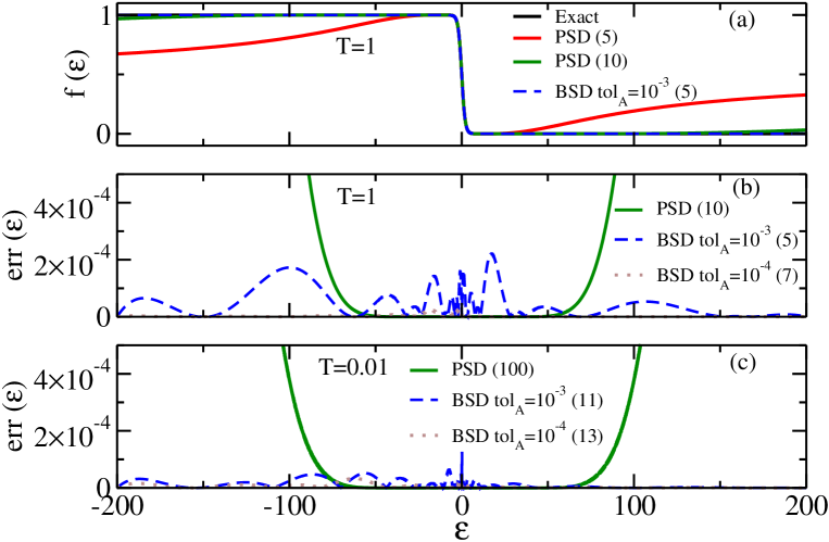
Figure 1: Performance of the BSD scheme to approximate the Fermi function $f(\varepsilon)=1/(1+e^{\beta\varepsilon})$ (here $k_{B}\equiv 1,\hbar\equiv 1$), compared with the conventional PSD scheme. Panel (a) shows the approximate Fermi functions using different schemes at $T=1$. The number in the parentheses is the number of basis functions $K_{f}$. Panels (b) and (c) present the error defined as $err(\varepsilon)=|f^{BSD/PSD}(\varepsilon)-f(\varepsilon)|$ for different schemes, at $T=1$ and $T=0.01$, respectively. Here, in the BSD using the AAA algorithm, the sample points are obtained in the domain $\mathcal{D}=[-200,200]$ with sufficiently dense discretization, the accuracy control parameter is given by $tol_{A}$.

Fig. 1 shows the performance of the BSD scheme to decompose the Fermi function $f(\varepsilon)=1/(1+e^{\beta\varepsilon})$ (here $k_{B}\equiv 1,\hbar\equiv 1$) at different temperatures, compared with the conventional PSD scheme. In Fig. 1(a) at $T=1$, the approximate function obtained from the PSD scheme shows high accuracy at small $\varepsilon$, but it deviates significantly from the exact curve at large $\varepsilon$. As the number of PSD basis functions increases, the accuracy improves and the deviation from the exact curve occurs at much larger $\varepsilon$. Since there is usually a finite range for the hybridization function $\Gamma_{\alpha,l}(\varepsilon)$, it is usually not a problem in decomposing the reservoir correlation functions, as the deviation of PSD approximation from $\Gamma_{\alpha,l}(\varepsilon)f_{l}^{\sigma}(\varepsilon)$ becomes smaller and smaller with larger numbers of basis function. The corresponding reservoir correlation function $C^{\sigma}_{\alpha l}(t)$ obtained from the PSD scheme then approaches the exact result, allowing systematic convergence of the HEOM.

The approximate distribution from the BSD scheme is more accurate than the PSD with the same number of basis functions. For $tol_{A}=10^{-3}$, the deviation of the BSD curve from the exact curve is barely noticeable on the curves shown in Fig. 1(a). Fig. 1(b) shows the error at $T=1$, the BSD errors oscillates at small $\varepsilon$, and the maximum error does not exceed $tol_{A}$. Fig. 1(c) shows the error at low temperature $T=0.01$. For the PSD scheme, the convergence slows down as the temperature decreases, and the PSD requires nearly 10 times as many basis functions as the $T=1$ case to reach similar accuracy. This severely limits the application of the PSD-based HEOM at low temperatures. However, for the BSD scheme, the number of required basis functions increases only slightly as the temperature decreases, with $K_{f}=5$ for $T=1$ and $K_{f}=11$ for $T=0.01$, when $tol_{A}=10^{-3}$. This behavior greatly reduces the number of basis functions required for low-temperature simulations, indicating the superiority of the BSD scheme at low temperatures. In addition, both the $T=1$ and $T=0.01$ cases show that the number of required basis functions only increases slightly as the accuracy increases (by decreasing $tol_{A}$), thus allowing for systematic convergence to numerically exact results.

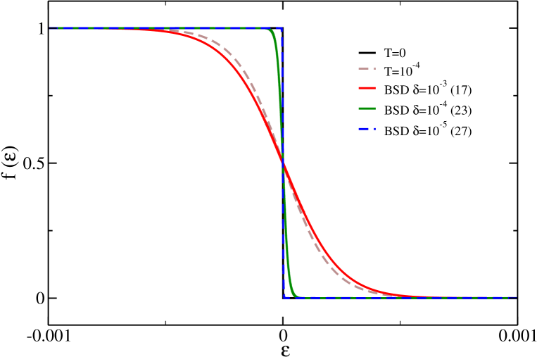
Figure 2: Performance of the BSD scheme to approximate the Fermi function $f(\varepsilon)=1/(1+e^{\beta\varepsilon})$ (here, $k_{B}\equiv 1,\hbar\equiv 1$) at $T=0$. The BSD results are shown for different minimum discretization intervals $\delta_{F}$. The exact $T=0$ and $T=10^{-4}$ Fermi functions are also shown for comparison. The sample points are obtained by discreting the domain $\mathcal{D}=[-200,200]$, and the accuracy control parameters is $tol_{A}=10^{-3}$. The number of basis functions $K_{f}$ is given in the parentheses.

Fig. 2 shows the performance of the BSD scheme when setting $T=0$. In this case, the Fermi distribution becomes a step function. We present the BSD results for different minimum discretization intervals $\delta_{F}$, where the discretization domain is $\mathcal{D}=[-200,200]$ with $tol_{A}=10^{-3}$. It can be seen that, the BSD results are affected by the interval between the points where the Fermi function jumps. And $K_{f}$ increases when decreasing $\delta_{F}$: $K_{f}=$17, 23, 27 for $\delta_{F}=10^{-3},10^{-4},10^{-5}$, respectively. We find that the BSD approximate results can only reach the step function asymptotically, and correspond to a temperature approximately one-tenth of the discretization interval (see the comparison between the $\delta_{F}=10^{-3}$ curve and the Fermi function at $T=10^{-4}$).

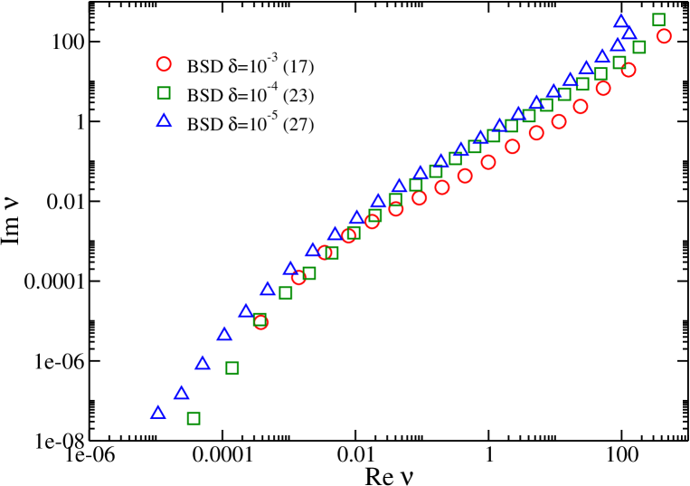
Figure 3: Distribution of real and imaginary parts of the poles in the upper half plane, i.e., $\nu^{f+}_{j}$ in Eq. (19) (we omit the $\alpha$ or $l$ subscripts here), for the BSD results in Fig. 2.

Fig. 3 shows distribution of the real and imaginary parts of the complex frequencies $\nu^{f+}_{\alpha lj}$ with different $\delta_{F}$. It can be seen that, the largest frequency originates from the boundary of discretization, and the smallest frequency is on the same order of the minimum interval, which corresponds to an effective very small temperature. The frequencies are nearly uniformly distributed on the logarithmic scale, confirming the moderate increase of $K_{f}$ when decreasing $\delta_{F}$.

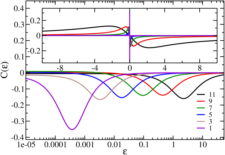
Figure 4: The spectrum of BSD basis functions $C_{j}(\varepsilon)$ ($2{\rm Re}\frac{d^{f+}_{j}}{i\varepsilon+\nu^{f+}_{j}}$) for $\delta_{F}=10^{-3}$ and $T=0$ as in Fig. 2. To calculate the coupling strength $d^{f+}_{j}$ using Eq. (20b), an auxiliary Lorentzian type hybridization function is chosen, with parameters $\eta=1$, $\gamma=10$, and $\varepsilon^{0}=0$ (the $\alpha$ and $l$ scripts are omitted). The basis functions are sorted in ascending order of ${\rm Re}\nu^{f+}_{j}$, from $j=1$ to $j=17$, the number in the legend indicates the $j$th basis functions. For simplicity, only the spectra for six low-frequency basis functions are shown. The inset shows the spectra in linear scale for the $\varepsilon$-axis.

We further characterize this logarithmic distributed BSD pole structure by plotting $C_{j}(\varepsilon)$ in Fig. 4, where $C_{j}(\varepsilon)=2{\rm Re}\frac{d^{f+}_{j}}{i\varepsilon+\nu^{f+}_{j}}$ is the spectrum of different BSD basis functions [note that $\sum_{j}C_{j}(\varepsilon)=\Gamma{(\varepsilon)}f^{+}(\varepsilon)$ with scripts $\alpha$ and $l$ omitted]. By assuming that $\nu^{f+}_{j}$ are arranged in ascending order, we show the results for the 1st, 3rd, 5th, 7th, 9th, and 11th poles, for $\delta_{F}=10^{-3}$ and $T=0$. The results show almost linearly distributed frequencies on the logarithmic scale. Compared with the nearly $1/T$ growth for Matsubara [i.e. $(2n+1)\pi/\beta$] or Padé basis functions, the number of basis functions from the BSD increases almost linearly as the temperature decreases exponentially. This makes the BSD scheme advantageous when performing very low temperature simulations. This behavior is also similar to the logarithmic discretization in the NRG framework Bulla et al. (2008), where $C_{j}(\varepsilon)$s replaces the discrete states in the NRG. However, since each $C_{j}(\varepsilon)$ includes a distribution of frequencies, the long-time dynamics of HEOM do not suffer from the discretization effect in the NRG approach Anders and Schiller (2005); Žitko and Pruschke (2009).

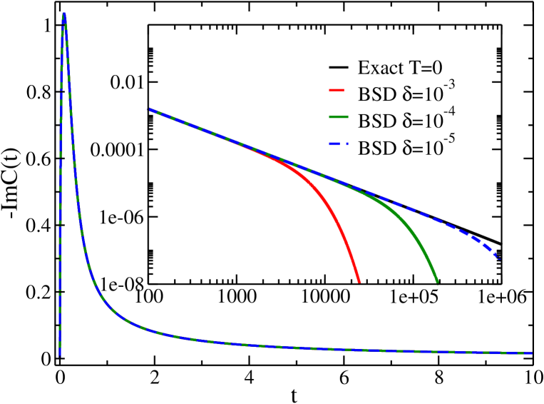
Figure 5: The reservoir correlation function $C(t)$ for the approximate BSD Fermi functions in Fig. 2. An auxiliary Lorentzian type hybridization function is chosen, with parameters $\eta=1$, $\gamma=10$, and $\varepsilon^{0}=0$ (the $\alpha$ and $l$ scripts are omitted). The other parameters are the same as in Fig. 2. For simplicity only $-{\rm Im}C^{+}(t)$ is shown.

Though the analytic form of the Fermi function at $T=0$ cannot be obtained directly from the BSD, the approximate distribution function can approach the $T=0$ results as we decrease the discretization interval and introduce more low-frequency terms. It is found that the weights [$d^{f\sigma}_{\alpha lj}$ in Eq. (19)] associated with low-frequencies are also very small, so the low-frequency term will contribute to the dynamics only when $\nu^{f+}_{\alpha lj}t\gg 1$ for all the high-frequency terms $\nu^{f+}_{\alpha lj}$. This is illustrated in Fig. 5, where we show the corresponding $C(t)$ for the approximate BSD Fermi functions in Fig. 2. To draw the reservoir correlation function $C(t)$, a hybridization function with Lorentzian type [defined later in Eq. (21)] is chosen with $\eta=1$, $\gamma=10$, $\varepsilon^{0}=0$ (here we omit the lead label $l$). For this hybridization function and with the Fermi energy $\mu=0$, the real part of $C(t)$ shows single exponential decay and only the imaginary part is affected by the temperature Chen et al. (2022). For simplicity, we only show $-{\rm Im}~{}C^{+}(t)$ in Fig. 5. It can be seen from Fig. 5 that, in the short time region, all the $C(t)$ curves are the same for different BSD discretization intervals $\delta_{F}$. The deviation from the exact $T=0$ curve only occurs at longer times, which is shown in the inset. For minimum discretization intervals $\delta_{F}=10^{-3},10^{-4}$, and $10^{-5}$, the deviation appears at approximately $t=10^{3},10^{4}$, and $10^{5}$, respectively.

From the above results, one can assume that the $T=0$ results can be obtained using the BSD scheme for a given accuracy. With the increase of the number of basis functions, we find that the weight $d^{f\sigma}_{\alpha lj}$ of the introduced low-frequency mode gets very small, such that its effect on the dynamics is very small before reaching a very long simulation time. This observation can also be understood from a different perspective: From Fig. 5, $C(t)$ obtained from the BSD scheme is the same as the zero temperature result till a long time $t\sim\delta_{F}^{-1}$, so one can assume that the dynamics represent the “true” zero temperature result till this time. For short-time simulations, or if the dissipation is relatively fast such that the system reaches its steady state before $\delta_{F}^{-1}$, the simulated dynamics is essentially at $T=0$. In practice, we will show later that, for the transport dynamics of the AIM, the result obtained from BSD with a small $\delta_{F}$ can converge and reproduce the correct zero temperature dynamics.

III.2 Low temperature dynamics with the Lorentzian hybridization function

We first consider the Lorentzian type hybridization function that has been employed in many recent studies Jin et al. (2008); Li et al. (2012); Härtle et al. (2015); Xu et al. (2017); Zhang et al. (2020); Dan et al. (2022), where

$$\Gamma_{\alpha,l}(\varepsilon)=\frac{\eta_{l}\gamma_{l}^{2}}{(\varepsilon-\varepsilon^{0}_{l})^{2}+\gamma_{l}^{2}}\;\;.$$ (21)

Here, $\varepsilon^{0}_{l}$ and $\gamma_{l}$ denote the band center and width of the lead $l$, and $\eta_{l}$ is the coupling strength between the molecule and the lead $l$. This form of hybridization function only has two simple poles that are symmetric with respect to the real axis, leading to $K_{\Gamma}=1$ in Eq. (19). The majority of the exponential terms in Eq. (6) thus originates from the BSD decomposition of the Fermi function.

To illustrate the numerical stability of the HEOM combined with the BSD scheme, we first calculate the voltage-driven dynamics of the AIM. In the low-temperature regime, due to the interplay between the quantum coherence and the Kondo resonance, the real-time dynamics exhibit nontrivial memory effects Zheng et al. (2013). As shown by Zheng et al. Zheng et al. (2013), driven by an external periodic voltage, the corresponding $I-V$ curve show hysteresis and self-crossing feature. In a later work, by using the FSD-based HEOM, it was shown that much stronger memory effects can be observed at even lower temperatures Zhang et al. (2020). However, the FSD has an asymptotic instability problem Zhang et al. (2020), and the time-dependent current start to diverge after a certain time. It was also shown that the instability becomes more severe when increasing the truncation tier $N_{\rm{trun}}$ of HEOM Zhang et al. (2020).

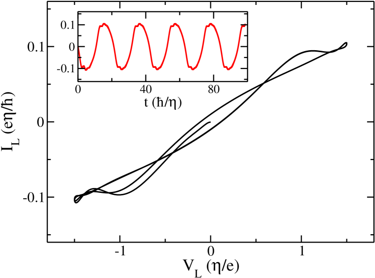
Figure 6: Dynamic $I-V$ characteristics for the AIM with the Lorentzian hybridization function, with an $ac$ driving voltage $V_{L}(t)=-V_{R}(t)=V_{0}\sin(\omega_{0}t)$. The parameters are (in units of $\eta$), $k_{B}T=0.05$, $\mu_{L}=\mu_{R}=0$, $\eta_{L}=\eta_{R}=1$, $\gamma_{L}=\gamma_{R}=20$, $\varepsilon^{0}_{L}=\varepsilon^{0}_{R}=0$, $\varepsilon_{\uparrow}=\varepsilon_{\downarrow}=-6$, $U=12$, $eV_{0}=1.5$, and $\hbar\omega_{0}=0.3$. Here, the BSD scheme is used to obtain the optimized pole structure of the Fermi function, with discretization domain $\mathcal{D}=[-200,200]$ and the accuracy control parameter $tol_{A}=10^{-3}$. $K_{f}=9$ basis functions are used to decompose the Fermi function at this temperature. The inset shows the corresponding transient current flow out of left lead $I_{L}(t)$. All simulations are performed using the on-the-fly filtering algorithm with the HEOM truncation level $N_{\rm{trun}}=5$.

Fig. 6 shows the dynamic $I-V$ characteristics for the same parameter of Fig. 3 in Ref. Zhang et al. (2020), where, in units of $\eta$, $k_{B}T=0.05$, $\mu_{L}=\mu_{R}=0$, $\eta_{L}=\eta_{R}=1$, $\gamma_{L}=\gamma_{R}=20$, $\varepsilon^{0}_{L}=\varepsilon^{0}_{R}=0$, $\varepsilon_{\uparrow}=\varepsilon_{\downarrow}=-6$, $U=12$, and the $ac$ voltage is $V_{L}(t)=-V_{R}(t)=V_{0}\sin(\omega_{0}t)$ with $eV_{0}=1.5$, $\hbar\omega_{0}=0.3$. Here, the truncation tier is set to $N_{\rm{trun}}=5$ that ensures convergence. At this temperature, the BSD scheme using the AAA algorithm gives $K_{f}=9$, when discretizing the Fermi functions dense enough in the domain $\mathcal{D}=[-200,200]$, and setting $tol_{A}=10^{-3}$.

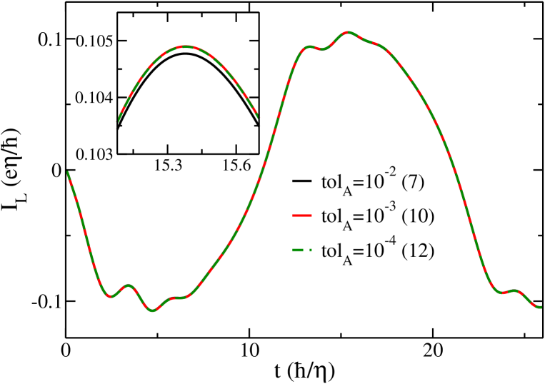
Figure 7: Transient current flow out of the left lead $I_{L}(t)$, with different BSD accuracy control parameter $tol_{A}$. All other parameters are the same as those in Fig. 6. The number in the parentheses denotes the total number of basis functions $K_{\Gamma}+K_{f}$ used in the simulation. The inset shows the curves near the peak current.

To obtain the transport current, we first propagate the total system without voltage ($\mu_{L}=\mu_{R}=0$) till equilibrium, then apply the $ac$ voltage to the left and right leads and propagate the system using Eq. (7). Finally, the transient current is calculated by Eq. (9). It can be seen in Fig. 6 that, the $I-V$ characteristics are in excellent agreement with the results in Ref. Zhang et al. (2020). The inset shows the real-time current dynamics. For longer simulations, the hysteresis loop is almost unchanged, as the $I-V$ curve repeats the earlier cycles. It can be seen that the current has a phase shift relative to the driving voltage, and due to the Kondo resonance, there are also overtone responses. These two features manifest themselves in the hysteresis behavior with multiple self-crossing points of $I-V$ characteristics Zheng et al. (2013). Moreover, the current dynamics obtained from BSD-based HEOM runs smoothly over $100~{}\hbar/\eta$, compared with the FSD-based HEOM that diverges at about $3~{}\hbar/\eta$ for $N_{\rm{trun}}=5$ Zhang et al. (2020), showing the long-time stability of the BSD scheme. We further use this example to demonstrate the accuracy of the BSD scheme. In Fig. 7, we show the convergence of the transient current with respect to the BSD tolerance parameter $tol_{A}$. The other parameters are the same as Fig. 6. For $tol_{A}=10^{-2},10^{-3},10^{-4}$, the number of basis functions to decompose the Fermi function is ${K_{f}}=$ 6, 9, and 11, respectively (note that $K_{\Gamma}=1$ for the Lorentzian hybridization function, and the number in the figure legend denotes $K_{\Gamma}+{K_{f}}$). It can be seen that, even with a relatively rough precision control parameter $tol_{A}=10^{-2}$, the dynamics are very close to convergence. This shows that the BSD scheme has high precision and $tol_{A}$ in the AAA algorithm is an effective precision control parameter. For $tol_{A}=10^{-3}$, the transient current is essentially indistinguishable from those with $tol_{A}=10^{-4}$. Based on these observations, we choose $tol_{A}=10^{-3}$ in later simulations.

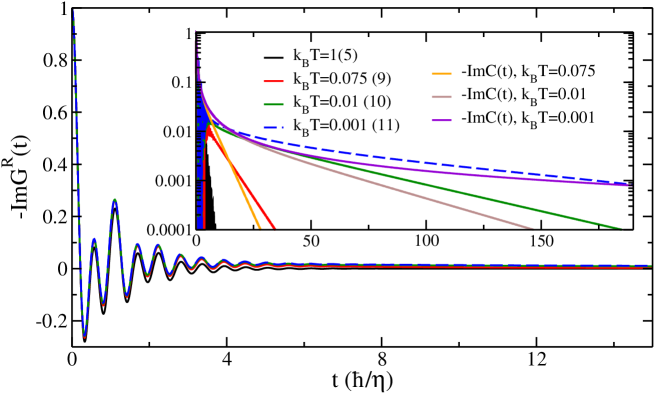
Figure 8: Imaginary part of the retarded Green’s function $-{\rm Im}G^{R}(t)$ for the AIM with Lorentzian hybridization function at different temperatures. The inset shows the long-time decay, where the imaginary parts of the reservoir correlation function $-{\rm Im}C^{+}_{L}(t)$ (in units of $\eta^{2}/\hbar$) at different temperatures are also shown for comparison. The parameters are, in units of $\eta$, $\eta_{L}=\eta_{R}=1$, $\gamma_{L}=\gamma_{R}=10$, $\varepsilon^{0}_{L}=\varepsilon^{0}_{R}=0$, $\mu_{L}=\mu_{R}=0$, $\varepsilon_{\uparrow}=\varepsilon_{\downarrow}=-5$, and $U=15$. The truncation tier of HEOM is set to $N_{\rm{trun}}=6$, and the number of basis functions $K_{\Gamma}+K_{f}$ used in the simulations is 5, 9, 10, 11 for $k_{B}T$=1, 0.075, 0.01, and 0.001, respectively. These numbers are also shown in the parentheses of the legends. In performing the BSD, the discretization domain for the Fermi distribution is $\mathcal{D}=[-200,200]$, and the accuracy control parameter is $tol_{A}=10^{-3}$.

Fig. 8 shows the Green’s function $G^{R}_{\alpha}(t)$ in Eq. (11), due to the similar behavior of ${\rm Im}G_{\alpha}^{R}(t)$ and ${\rm Re}G_{\alpha}^{R}(t)$, only $-{\rm Im}G_{\alpha}^{R}(t)$ [i.e., ${\rm Re}\langle\{\hat{a}_{\alpha}(t),\hat{a}_{\alpha}^{\dagger}\}\rangle$] is shown for simplicity. We choose the same system parameters studied previously with the PSD- Li et al. (2012) and FSD-based HEOM Zhang et al. (2020). That is, in units of $\eta$, $\eta_{L}=\eta_{R}=1$, $\gamma_{L}=\gamma_{R}=10$, $\varepsilon^{0}_{L}=\varepsilon^{0}_{R}=0$, $\mu_{L}=\mu_{R}=0$, and $\varepsilon_{\uparrow}=\varepsilon_{\downarrow}=-5$, $U=15$. The two spin states are now degenerate and we drop the subscript $\alpha$ for the spin DOF. Since parameters for the left and right leads are the same, we can combine them into a single lead with $\eta_{tot}=\eta_{L}+\eta_{R}$, and the number of basis functions in the HEOM can be greatly reduced. Our data are calculated using HEOM truncated at $N_{\rm{trun}}=6$ to ensure convergence. In the BSD scheme using the AAA algorithm, the Fermi distribution is discretized in the range $\mathcal{D}=[-200,200]$, and $tol_{A}=10^{-3}$, which leads to the number of basis functions $K_{\Gamma}+K_{f}=$ 5, 9, 10, 11 for $k_{B}T=$ 1, 0.075, 0.01, 0.001, respectively.

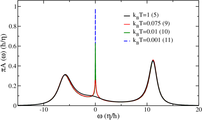
Figure 9: The impurity spectral function $A(\omega)$ calculated from $G^{R}(t)$ in Fig. 8 through Eq. (10) at different temperatures. All the parameters are the same as those in Fig. 8.

The retarded Green’s function is calculated after propagating the system to equilibrium, which oscillates over short period of time and shows exponential decay at longer times. This exponential decay is typical for Green’s function at longer times Barthel et al. (2009); Wolf et al. (2015a, b). For comparison, we also plot the imaginary part of the reservoir correlation function $-{\rm Im}C^{+}_{L}(t)$ (in units of $\eta^{2}/\hbar$) in the inset. It can be seen that the long-time decay of the Green’s function is essentially determined by the low-frequency effective mode of the reservoir correlation function at this temperature, which is responsible for the sharp peak of $A(\omega)$ near the Fermi energy as the indication of Kondo resonance (see Fig. 9). As the temperature decreases, the slope of $-{\rm Im}C^{+}_{L}(t)$ and $-{\rm Im}G^{R}(t)$ becomes closer, and they decay slowly such that longer simulation is required. For $k_{B}T=$ 0.001, we simulate the Green’s function to the exponential decay regime (about $t=200~{}\hbar/\eta$ in the inset) and then employ the “linear prediction” method White and Affleck (2008); Barthel et al. (2009); Ganahl et al. (2015) to extrapolate the simulation data to longer times.

Fig. 9 shows the spectral functions at various temperatures. The spectral function $A(\omega)$ is obtained from the imaginary part of the Fourier transform of $G^{R}(t)$, that is, Eq.(10). For $k_{B}T=$ 1.0, 0.075, and 0.01, respectively, the results are consistent with those in Ref. Zhang et al. (2020). The spectral function $A(\omega)$ shows two broad peaks at impurity level energies $\varepsilon$ and $\varepsilon+U$, which do not change significantly with the temperature. This is because the broadening is caused by coupling to the leads, such that it is on the order of $\eta$ and is only slightly affected by temperature. On the other hand, the peak located at the Fermi energy is significantly affected by decreasing the temperature. A sharp peak at the Fermi energy appears at low temperature, and for $T=0.001$, the amplitude of this peak is very close to 1, which agrees with the theoretical result at $T=0$ Langreth (1966); Martinek et al. (2003).

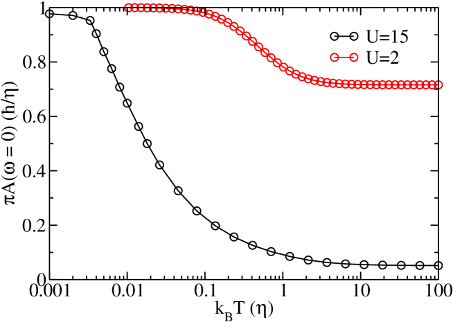
Figure 10: The calculated $A(\omega=0)$ at various temperatures with $N_{\rm{trun}}=6$. The black circles labeled with $U=15$ are obtained using the same parameters as those in Fig. 8. The red circles labeled with $U=2$ assume a symmetric AIM (in units of $\eta$, $\varepsilon_{\uparrow}=\varepsilon_{\downarrow}=-U/2=-1$, with all other parameters the same as those in Fig. 8). The Friedel sum rule predicts $A(0)=1$ at $T=0$ for the symmetric AIM.

We also compare our BSD-HEOM result to the analytic Friedel sum rule Langreth (1966); Martinek et al. (2003) at zero temperature, which is given by ${\pi}A(\omega=0)\eta/\hbar=\sin^{2}(\pi n_{\alpha})$, with $n_{\alpha}=\langle\hat{a}_{\alpha}^{{\dagger}}\hat{a}_{\alpha}\rangle$. Fig. 10 shows the calculated $A(\omega=0)$ at different temperatures, with $N_{\rm{trun}}=6$. The red circle in Fig. 10 corresponds to a symmetric AIM case with a small Coulomb repulsive energy $U=2$ (in units of $\eta$), where the other parameters are the same as those in Fig. 8. For this symmetric AIM, at equilibrium, $n_{\alpha}=1/2$, the transition temperature (here we define it as the temperature at which the Kondo peak changed significantly) is about $k_{B}T=1$. As the temperature decreases, the amplitude of the Kondo peak, $\pi A(\omega=0)\eta/\hbar$ approaches 1, which verifies the Friedel sum rule and indicates the accuracy of our BSD-based HEOM.

The black circles in Fig. 10 show the result for the parameters in Fig. 8 with a larger Coulomb repulsive energy $U=15$. In this case, $n_{\alpha}$ at equilibrium for $T=0.001$ is 0.4811, and the Friedel sum rule predicts a Kondo peak amplitude at $T=0$ very close to 1. The transition temperature now is very low at about $k_{B}T=0.01$. We can also see that $A(\omega=0)$ approaches the analytic result as $T$ goes down. This indicates that the calculated data contains the correct long-time behavior and the extrapolation scheme works well in these cases.

It is also noted that the results below $k_{B}T=0.01$ are obtained by combining the long-time simulation data with the “linear prediction” method White and Affleck (2008); Barthel et al. (2009). To make the extrapolation procedure work, the HEOM needs to capture the correct dynamics till the asymptotic region where the extrapolation ansatz works, which depends on the long-time convergence of HEOM. It has been found previously that, when the truncation tier $N_{\rm{trun}}$ is not sufficient, HEOM does not converge and may cause overshoots of the Kondo peak Zhang et al. (2022); Ding et al. (2022). In more complex cases or as temperature decreased even further, a larger $N_{\rm{trun}}$ might be needed for the convergence of HEOM.

III.3 Low temperature dynamics with the tight-binding hybridization function

To illustrate that the BSD scheme can handle general forms of hybridization function, in this section we choose a tight-binding hybridization function with $\Gamma_{\alpha,l}(\varepsilon)$ given by:

$$\Gamma(\varepsilon)=\begin{cases}\frac{\Delta_{e}^{2}}{W_{e}^{2}}\sqrt{4W_{e}^{2}-\varepsilon^{2}}&|\varepsilon|<=2|W_{e}|\\ 0&|\varepsilon|>2|W_{e}|\end{cases},\\$$ (22a)

$$\Gamma_{\alpha,L}(\varepsilon)=\Gamma(\varepsilon-\mu_{L}),\quad\Gamma_{\alpha,R}(\varepsilon)=\Gamma(\varepsilon-\mu_{R})\;\;.$$ (22b)

This semi-elliptical form of hybridization function has been studied previously by Wang et al. Wang and Thoss (2009, 2013), Wolf et al. Wolf et al. (2014, 2015a), and other groups Karski et al. (2008); Dorda et al. (2014); Wójtowicz et al. (2021); Kohn and Santoro (2021). Wang et al. have used the ML-MCTDH-SQR method to explore charge transport dynamics through single-molecule junctions at zero temperature. Here, we fix $\Delta_{e}=0.2~{}eV$ and $W_{e}=1~{}eV$ which are the same as those in Ref. Wang and Thoss (2013). As in the previous section, we set the two spin states to be degenerate.

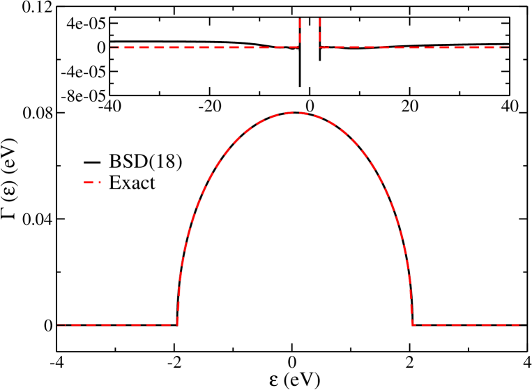
Figure 11: Performance of the BSD scheme for decomposing the tight-binding hybridization function $\Gamma(\varepsilon)$ defined in Eq. (22), with $\Delta_{e}=0.2~{}eV$ and $W_{e}=1~{}eV$. $\Gamma(E)$ is discretized in the domain $\mathcal{D}_{\Gamma}=[-7~{}eV,7~{}eV]$, with the minimum discretization interval $\delta_{\Gamma}=0.003~{}eV$ near the band edge. The accuracy control parameter $tol_{A}=10^{-3}$ results in $K_{\Gamma}=18$. The inset shows the error of the BSD scheme, for the range close to the band edge and beyond the discretization domain $\mathcal{D}$.

Fig. 11 shows the performance of the BSD scheme for decomposing the tight-binding hybridization function $\Gamma(E)$ defined in Eq. (22). In the BSD scheme using the AAA algorithm, we set $tol_{A}=10^{-3}$ and discretize the hybridization function on the domain $\mathcal{D}=[-7~{}eV,7~{}eV]$, with the minimum discretization interval $\delta_{\Gamma}=0.003~{}eV$. This results in $K_{\Gamma}=18$ for the semi-elliptical hybridization function. It can be seen that the approximate hybridization function agrees very well with the exact one, even beyond the fitting range (see the inset). From the inset, we can also see that the approximate hybridization function deviates from the exact one mainly on the hard edges, and places beyond the fitting domain. But the overall errors are smaller than the given accuracy control parameter $tol_{A}$.

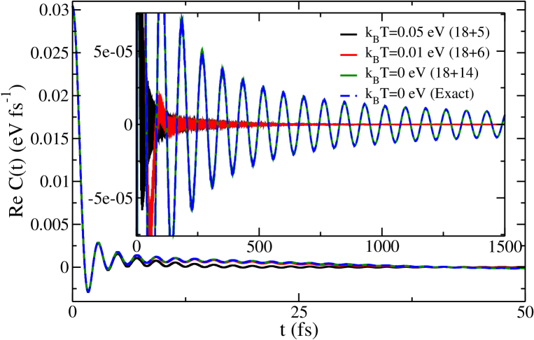
Figure 12: The reservoir correlation function $C_{L}^{+}(t)$ at different temperatures, for $\Gamma(\varepsilon)$ in Fig. 11. For simplicity, only the real part is presented. Here, $\mu_{L}=0.05~{}eV$, $\Gamma_{L}(\varepsilon)=\Gamma(\varepsilon-\mu_{L})$, and the Fermi functions are discretized in the domain $\mathcal{D}_{f}=[-3~{}eV,3~{}eV]$, with $tol_{A}=10^{-3}$. For $T=0$, the minimum discretization interval $\delta_{F}$ is $10^{-4}~{}eV$. The number of basis functions used to decompose the Fermi function is $K_{f}=$ 5, 6, 14 for $k_{B}T=$ 0.05, 0.01, and 0 eV, respectively. The inset shows the long-time behavior.

Fig. 12 shows the corresponding reservoir correlation function, calculated from $\Gamma(E)$ in Fig. 11, at different temperatures $k_{B}T=$ 0.05, 0.01, and 0 eV with the source-drain voltage applied symmetrically to the left and right lead $\mu_{L}=-\mu_{R}=0.05~{}eV$. For simplicity, only the real part of $C_{L}^{+}(t)$ is shown. The BSD scheme results in $K_{f}=$ 5, 6, and 14 for $k_{B}T=$ 0.05, 0.01, and 0 eV, respectively. Compared with the Lorentzian hybridization function, the tight-binding hybridization function results in oscillating reservoir correlation functions with the frequency associated with bandwidth. The hard edge of the tight-binding hybridization function, like the Fermi function at $T=0$ shown in Fig. 2, leads to many poles with small decay constants ${\rm Re}\nu^{\Gamma+}_{Lj}$ and weights $d^{\Gamma+}_{Lj}$. The minimum ${\rm Re}\nu^{\Gamma+}_{Lj}$ is found to be slightly smaller than $\delta_{\Gamma}$.

When the minimum ${\rm Re}\nu^{f+}_{Lj}$ from the Fermi distribution is larger than the minimum ${\rm Re}\nu^{\Gamma+}_{Lj}$, the decay of $C_{L}^{+}(t)$ is controlled by temperature at short time, and is controlled by the basis functions obtained from the tight-binding hybridization function at longer time. This is shown in $k_{B}T=0.05~{}eV$ and $k_{B}T=0.01~{}eV$ curves. At short time, the decay of the high-temperature $k_{B}T=0.05~{}eV$ correlation function is faster than the low-temperature one at $k_{B}T=0.01~{}eV$. But at longer times, the two curves almost coincide as shown in the inset of Fig. 12. When the temperature is low enough, the decay of $C_{L}^{+}(t)$ is mainly controlled by the temperature. Indeed, the approximate $C_{L}^{+}(t)$ with $T=0$ obtained with $\delta_{F}=10^{-4}~{}eV$ shows rather different long-time behavior.

Although as discussed previously in Sec. III.1, the approximate $C_{L}^{+}(t)$ corresponds to a very small effective temperature as shown in Fig. 2, it can be seen from the inset of Fig. 12 that, the approximate and exact correlation functions agree with each other over a very long time range. In this sense, we can conclude that within this time range, the dynamics obtained from the approximate $C_{L}^{+}(t)$ should essentially be the same as the “true” zero temperature dynamics at $T=0$. Moreover, though not shown in the figure, in the temperature-controlled decay regime, the decay rate of the reservoir correlation function is the same for different forms of hybridization functions, which will result in the same decay rate of the Green’s function as in Fig. 8, such that the Kondo resonance of different types of hybridization functions at low temperature should not change significantly Chen et al. (2022).

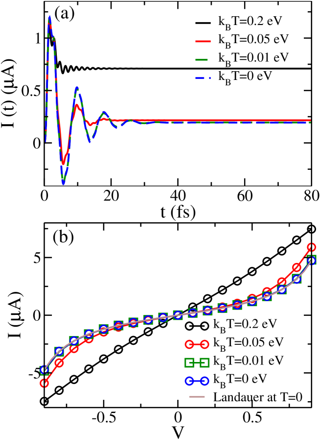
Figure 13: (a) The average current $I(t)=[I_{L}(t)-I_{R}(t)]/2$ of the non-interacting AIM ($U$=0) with the tight-binding hybridization function at different temperatures. Here, $\Delta_{e}=0.2~{}eV$, $W_{e}=1~{}eV$, $\epsilon_{\alpha}=-0.5~{}eV$, $U=0$, and the bias voltage $V=0.1{~{}\rm V}$ is symmetrically applied to two leads: $\mu_{L}=-\mu_{R}=V/2$. The BSD result is the same as in Fig. 12, with $K_{\Gamma}=18$, $K_{f}=$ 5, 6, 14 for $k_{B}T=$ 0.05, 0.01, $0~{}eV$, respectively. The $k_{B}T=0.2~{}eV$ case ($K_{f}=3$), though at an unrealistic high temperature, is also shown for comparison. (b) The average steady state current at different bias voltage, the other parameters are same as those in panel (a).

We then study the current dynamics of the AIM with the tight-binding hybridization function at different temperatures. Fig. 13 shows the current dynamics for the non-interacting case $U=0$. In this case, the HEOM with $N_{\rm{trun}}=2$ leads to exact results Jin et al. (2008). The energy of the system state is $\varepsilon_{\alpha}=-0.5~{}eV$, $\mu_{L}=-\mu_{R}=0.05~{}eV$ such that the bias voltage is $0.1~{}{\rm V}$. This parameter corresponds to the so called off-resonant transport regime Wang and Thoss (2013). The other parameters for the hybridization or Fermi functions are the same as those in Fig. 12. In the simulation, the initial system state is doubly occupied. In this case, the current shows transient oscillations at short time that decay due to the coupling to the leads. When the temperature is relatively high, we can see another high-frequency oscillation with frequency $\omega\approx 3~{}fs^{-1}$ ($2~{}eV$) which corresponds to the band edge of the semi-elliptical hybridization function.

At low temperatures, the lead states at the band edge do not contribute to the transport process. So as the temperature decreases, the high-frequency oscillation is suppressed. The steady state current is suppressed as the temperature decreases, since the conductive window is reduced. As can be seen from Fig. 13(a), the $k_{B}T=0.01~{}eV$ result is already very close to that at $T=0$, indicating that the system is already in the low temperature regime. Further lowering the temperature will only lead to very minor changes of the dynamics. Moreover, our $T=0$ results obtained from the BSD scheme agree well with the results in Ref. Wang and Thoss (2013).

Fig. 13(b) gives the steady state current as a function of the bias voltage, with all other parameters fixed. At high temperature $k_{B}T=0.2~{}eV$, the $I-V$ characteristics at this bias range in almost linear. When lowering the temperature, the conductance increases after entering the resonant transport regime. The $I-V$ curve is almost unchanged for the $k_{B}T=0.01~{}eV$ and $T=0$ cases obtained from the BSD-based HEOM, which further shows that $k_{B}T=0.01eV$ is already in the low temperature regime. It is noted that for the non-interacting case $U=0$, the stationary current can be obtained exactly from the Landauer-Büttiker formula Mahan (2000); Dan et al. (2022). As shown in Fig. 13(b), the BSD-based HEOM results at $T=0$ agrees well with those from the Landauer-Büttiker formula, indicating that the $T=0$ results are converged.

We then study the current dynamics of AIM in the presence of electron-electron repulsive energy $U$. This is much more challenging than the non-interacting case since the HEOM must be truncated at a higher tier. At low temperatures, the needed truncation tier for high accuracy is relatively high. Our traditional HEOM code based on the filtering approach can not handle the computational and memory costs to get converged results at $T=0$ ($K_{\Gamma}+K_{f}=32$), for truncation tier higher than $N_{\rm{trun}}=4$. In this case, we resort to the MPS-HEOM method Shi et al. (2018) to reduce the computational costs.

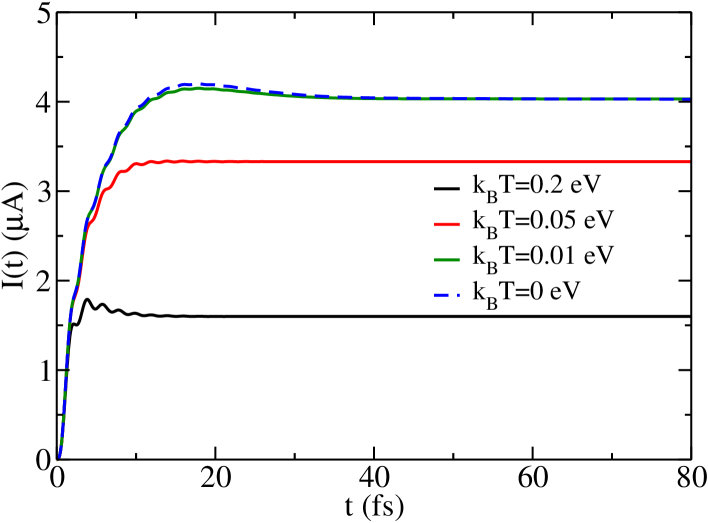
Figure 14: Time evolution of the average transport current of the AIM with the tight-binding hybridization function at different temperatures. The electron-electron repulsive energy is $U=0.5~{}eV$, all the other parameters are the same as those in Fig. 13(a). The $T=0$ result is obtained using MPS-HEOM with the maximum bond dimension up to 500.

Fig. 14 shows the current dynamics of the AIM with $U=0.5~{}eV$, with all the other parameters being the same as those in Fig. 13. Here the $T=0$ result is obtained using MPS-HEOM Shi et al. (2018) with maximum bond dimension up to 500. Comparing to Fig. 13(a), the $U=0.5~{}eV$ case has a larger current. This is because that, the energy change from the single occupied state to the doubly occupied state, $\varepsilon+U$, moves close to the Fermi energy and provides a channel for resonant transport. In the $U=0.5~{}eV$ case, the transport becomes incoherent for a short period of time. Moreover, the temperature dependence of the current is reversed, that is, decreasing the temperature results in an increase in the current. The reason is that, decreasing the temperature reduces the fluctuations, and increases the probability of resonant transport. It can be seen that, the high-frequency oscillation of the current which is the band edge effect appears even at low temperature. While in the $U=0$ case, this effect only appears at high temperatures. The $k_{B}T=0.01~{}eV$ case is found to be already in the low-temperature regime, where the dynamics are only slightly different from the $T=0$ result in the transient regime, and the steady-state currents are almost the same. Our $T=0$ results agree well with those in Ref. Wang and Thoss (2013), which verifies the validity of the BSD scheme for zero temperature dynamics. The relaxation process of the current to stationary value is also slower at low temperatures, due to the long time memory effect.

IV Conclusion and Discussion

In this paper, we have proposed to use the BSD scheme for the sum-over-poles decomposition of the Fermionic reservoir correlation functions. The BSD scheme based on rational function approximation of barycentric form can be used to calculate optimized pole structure than the analytical Matsubara and PSD poles, thus is superior in low-temperature simulations. This decomposition scheme is easy to implement with existing software packages. By approximating the reservoir correlation functions $C^{\sigma}_{\alpha,l}(t)$ and $C^{\bar{\sigma}}_{\alpha,l}(t)$ with the same set of poles, the traditional structure of the HEOM is also maintained. With the BSD scheme, we can apply the HEOM to the AIM in the low-temperature regime even at $T=0$ for dynamic simulation with high efficiency, accuracy, and long-time stability. The improvements of BSD over previous HEOM-based methods such as PSD Ozaki (2007); Hu et al. (2010, 2011) and FSD Cui et al. (2019); Zhang et al. (2020) in efficiency and long-time stability, as well as the ability to deal with arbitrary band structures, offer new opportunities for applications in lower temperatures or more realistic systems.

To demonstrate the performance of the BSD scheme, we first apply it to approximate the Fermi function, the results show that the number of required basis functions grows almost linearly as the temperature decreases exponentially, compared to the exponential growth of the widely used PSD scheme. The low temperature performance is further demonstrated by calculating the Kondo peak of the impurity spectral function of the AIM with the Lorentzian hybridization function. The $I-V$ characteristics under an $ac$ voltage have also been simulated, showing the accuracy and long-time stability of the HEOM combined with the BSD scheme. Furthermore, to illustrate the application to arbitrary band structures, we apply the BSD scheme to the AIM with a tight-binding band structure, where the hybridization function has no analytic poles. Combined with the MPS-HEOM Shi et al. (2018), the current dynamics at different temperatures and even at $T=0$ have been explored.

We have also pointed out that the BSD scheme cannot really reach the Fermi function at $T=0$ which is discontinuous at the Fermi energy. The approximate function for $T=0$ based on BSD can be regarded as the Fermi function at a very small temperature related to the smallest discretizing interval $\delta_{F}$. In the time domain, the simulated results based on BSD reflect the true $T=0$ dynamics within a time range determined by $1/\delta_{F}$ which in many cases can be chosen sufficiently large to approach the steady-state regime.

Compared to other widely used methods such as the QMC Mühlbacher and Rabani (2008); Werner et al. (2009); Schiró and Fabrizio (2009); Gull et al. (2011); Antipov et al. (2016); Krivenko et al. (2019); Cohen et al. (2015); Antipov et al. (2017) and time-dependent NRG (TD-NRG) Anders and Schiller (2005, 2006); Bulla et al. (2008); Nghiem and Costi (2018), the long-time dynamics of HEOM do not suffer from discretization problems, and its computation cost grows linearly as time increases. The BSD scheme in this work also significantly increases the capability of HEOM in the low-temperature regime and for more complex band structures. Thus, we believe that BSD-based HEOM could become the method of choice for certain types of applications, especially in long-time simulations that may be difficult for the QMC and TD-NRG methods.

Recently, some of us have developed the generalized master equation (GME) method to calculate the exact memory kernel from physical quantities such as population and current Dan et al. (2022). The memory kernels, which usually decay within a short period of time, can be used to produce reliable long-time dynamics Cohen and Rabani (2011); Cohen et al. (2013). Combining this method with the BSD scheme may allow us to calculate efficiently asymptotic long-time dynamics and stationary state properties at $T=0$ for even broader classes of hybridization functions.

With the development of the HEOM method and new algorithms including the MPS-HEOM Shi et al. (2018) with efficient time evolution methods Yang and White (2020); Borrelli and Dolgov (2021), Tree-Tensor HEOM Yan et al. (2021), and the hierarchical Schrödinger equations of motion (HSEOM) Nakamura and Tanimura (2018), the BSD scheme provides a new method for the simulation of realistic systems at low temperatures. Moreover, the methodology can be applied to other approaches based on an expansion of reservoir correlation functions or Green’s functions, such as the hierarchy of pure states (HOPS) Suess et al. (2014), the non-equilibrium Green’s function (NEGF) Beach et al. (2000); Croy and Saalmann (2009); Gu et al. (2020) methods, and the nonequilibrium dynamical mean-field theory (DMFT) Arrigoni et al. (2013).