Stability of long-sustained oscillations induced by electron tunneling

Abstract

Self-oscillations are the result of an efficient mechanism generating periodic motion from a constant power source. In quantum devices, these oscillations may arise due to the interaction between single electron dynamics and mechanical motion. Due to the complexity of this mechanism, these self-oscillations may irrupt, vanish, or exhibit a bistable behavior causing hysteresis cycles. We observe these hysteresis cycles and characterize the stability of different regimes in single and double quantum dot configurations. In particular cases, we find these oscillations stable for over 20 seconds, many orders of magnitude above electronic and mechanical characteristic timescales, revealing the robustness of the mechanism at play. The experimental results are reproduced by our theoretical model that provides a complete understanding of bistability in nanoelectromechanical devices.

Coupling of quantum devices to mechanical degrees of freedom can be exploited for high precision measurements [1, 2, 3, 4, 5, 6] and may serve as a platform for quantum and classical information processing [7, 8]. At low temperatures, carbon nanotube (CNT) devices can be operated as extremely sensitive mechanical oscillators which are strongly coupled to single electron tunneling [9, 10, 11, 12, 13, 14, 15, 16, 4, 17, 18]. The interplay between single electron tunneling and mechanical motion, in the absence of a mechanical drive, can give rise to self-sustained oscillations. Such self-oscillations were observed to be either present or absent depending on the electron transport regime, both in theory  [19, 20, 21, 22] and experiments  [23, 24, 25, 26, 27, 28, 29]. At the boundary between regimes, self-oscillations can appear or vanish spontaneously. These bistable states of motion of an undriven oscillator, until now unexplored, are of particular interest for applications of these devices in quantum and stochastic thermodynamics [30, 31, 32, 33], in collective dynamics and synchronization [34], and in emulating neural behavior [35, 36, 37].

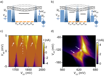
FIG. 1: a,b) Schematic of the device in single dot (a) and double dot (b) configurations. A CNT is suspended between the source and drain electrodes. Five gate voltages, $V_{\text{G1-G5}}$, are used to create either a single dot or a double dot. A bias voltage $V_{\text{SD}}$ drives a current $I$ through the CNT. The chemical potentials of the source and drain electrodes are $\mu_{\text{S}}=eV_{\text{SD}}$ and $\mu_{\text{D}}=0$, respectively. The right, left and interdot tunnel rates are indicated and the associated tunnel rates are labeled $\Gamma_{\text{R}}$, $\Gamma_{\text{L}}$ and $\Gamma_{\rm M}$. c) Current measured in single-dot configuration as a function of the gate voltage $V_{\text{G3}}$ and bias voltage $V_{\text{SD}}$. White arrows point at features which indicate the presence of self-oscillations. The current traces in Fig. 2(a) were taken along the dashed vertical line. d) Current measured in the double-dot configuration by sweeping $V_{\text{G5}}$ and stepping $V_{\text{G3}}$ with $V_{\text{SD}}=1.8$ mV. White arrows point at current features which indicate the presence of self-oscillations. The white star indicates a triple point, where we observe the switch in current as a function of $V_{\text{SD}}$ plotted in Fig. 4(a).

In this paper, we measure bistable self-oscillations both for single and double quantum dot configurations, and present a model that provides a complete characterization of the stability of self-oscillations at different bias voltages. In such stability diagrams, different bias voltage paths are navigated and thus different dynamics of the mechanical oscillator are accessed. We find that, once started, undriven oscillations can be self sustained for more than $10^{8}$ mechanical periods.

Our electromechanical device consists of a fully suspended CNT (see Fig. 1(a))  [38, 39, 27, 14]. A confining potential for charges is created within the nanotube by applying DC voltages to gate electrodes. Applying a bias voltage $V_{\text{SD}}$ between the source and drain electrodes, we measure a current $I$ through the CNT. The gate electrodes, to which we apply voltages $V_{\text{G1-5}}$, are located beneath the CNT. These gate voltages define an electrostatic potential for the confined charges, and depending on the combination of gate voltage values, we can define single or double quantum dots within the CNT (Figs. 1(a,b)). Single or double quantum dot configurations are identified by the observation of Coulomb diamonds or bias triangles, respectively [40, 41].

The mechanical motion of the CNT can be excited by applying a radio-frequency (rf) signal to one of the gate electrodes. Sharp changes in the current through the CNT indicate its mechanical motion [9, 42, 43], and we identify the natural mechanical resonance frequency $\Omega/2\pi=270$ MHz. At charge degeneracy points, strong coupling between electron tunneling and mechanical motion is evidenced by the softening of the mechanical resonance frequency [11, 23, 10, 12, 44, 14].

Self-oscillations are identified as sharp switches in current appearing in the absence of an rf excitation [23, 24, 25, 26, 27, 29]. In a single-dot configuration, we observe these switches on the left (right) flank of some of the Coulomb diamonds at positive (negative) bias (Fig. 1(c)). While in a double-dot configuration, these sharp switches are visible within the bias triangles (Fig. 1(d)). In the single-dot configuration, we observe the bistability through the hysteretic behavior of the current when sweeping $V_{\text{SD}}$ in and out of the self-oscillation area, following the vertical white dashed line in Fig. 1(c), which corresponds to a constant gate voltage $V_{\text{G3}}=1.8$ V. As $V_{\text{SD}}$ is swept upward, a sharp increase of current around $V_{\text{SD}}=2.3$ mV indicates the onset of self-oscillations (red curve in Fig. 2(a)). However, when $V_{\text{SD}}$ is swept in the opposite direction (blue curve), the sharp decrease of current is found at a significantly lower voltage $V_{\text{SD}}\simeq 1.3$ mV. The sharp changes in current are reproducible over several sweeps of $V_{\text{SD}}$, with a small variation in threshold voltages due to the stochastic nature of this process. This hysteresis cycle shows that there is a range of bias voltages, $V_{\text{SD}}\simeq 1.3-2.3$ mV, labeled as (II) in Fig. 2, for which the system exhibits bistability.

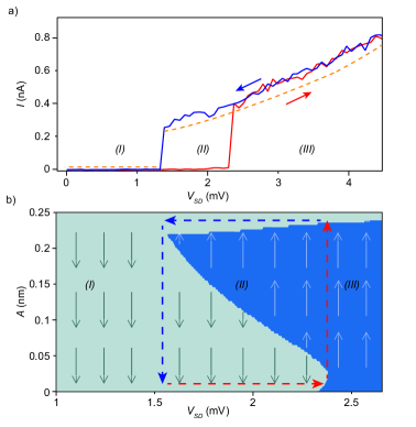
FIG. 2: a) Current switch hysteresis as a function of $V_{\text{SD}}$ measured in the single dot regime following the dashed line ($V_{\text{G3}}=1.8$ V) in Fig. 1(c). The red and blue arrows indicate the direction of each current sweep. The orange dashed line is the current calculated from Eq. (5). The numerals (I, II, III) indicate regions of no oscillations, bistability and self-oscillations, respectively. b) Stability diagram: the dark (light) blue areas indicate $\Delta E>0$ $(\Delta E<0)$ for different values of $A$ and $V_{\text{SD}}$. Small arrows indicate the direction in which $A$ would change in each area given the sign of $\Delta E$. Blue an red arrows delimit regions (I), (II) and (III) and indicate a similar hysteresis cycle as that shown in panel a). We use $\Omega/2\pi=270$ MHz, $g_{\rm m}=0.01$ eV$/$nm, $m=2\times 10^{-22}$ kg, and $Q=1000$, $\Gamma_{\text{L}}=400\leavevmode\nobreak\ \text{ GHz}$, $\Gamma_{\text{R}}=18\leavevmode\nobreak\ \text{ GHz}$, $\alpha_{\text{L}}=4\leavevmode\nobreak\ \text{ nm}^{-1}$, and $\alpha_{\text{R}}=0$.

We can explain the bistability regime observed using a model capturing the strong coupling between single-electron tunneling and mechanical motion [19, 20, 21]. The model describes the motion of the CNT as a single vibrational mode of displacement $x(t)$, frequency $\Omega$, and effective mass $m$, whose evolution equation reads

$$m\ddot{x}(t)=-m\Omega^{2}x(t)-\gamma\dot{x}(t)-g_{\rm m}n(t)$$ (1)

Here $\gamma$ is the friction coefficient that accounts for the different dissipation mechanisms affecting the CNT motion and $n(t)=0,1$ is the occupation number of the dot, which is a stochastic variable. Gate voltages exerts a force on the CNT when the dot is occupied, i.e. $n(t)=1$. This force depends on several parameters like the distance between the dot and the gate electrodes. For small oscillations, this force can be considered constant and is denoted by $g_{\rm m}$. The constant $g_{\rm m}$ determines the strength of the coupling between the dot charge and the mechanical degree of freedom. Finally, it is more convenient to express the friction coefficient as $\gamma={m\Omega}/{Q}$, in terms of the quality factor $Q$ of the oscillator, which can be measured using the linewidth of the resonator.

The stochastic occupation number $n(t)$ undergoes Poissonian jumps whenever an electron tunnels from the source/drain electrodes to the quantum dot or vice-versa [21, 31]. The rates of jumps from the left and right electrodes to the dot are given by $\Gamma_{\text{L,R}}(x)f_{\text{L,R}}(\epsilon(x))$ and from the dot to the electrodes by $\Gamma_{\text{L,R}}(x)[1-f_{\text{L,R}}(\epsilon(x))]$, where $\Gamma_{\text{L,R}}(x)$ are the tunneling rates, and $f_{\text{L,R}}(\epsilon(x))$ are the Fermi functions of each lead evaluated at the energy $\epsilon(x)$.The electrochemical potential of the dot, $\epsilon(x)=\epsilon_{0}+g_{\rm m}x$, depends on the displacement $x$ of the oscillation. The constant $\epsilon_{0}$ is the electrochemical potential of the dot in the absence of any mechanical motion. Assuming that the energy of the dot reaches the chemical potential $\mu_{\text{S}}$ at the onset of self-oscillations and transport, $\epsilon_{0}=eV^{*}_{\text{S}}$, where $V^{*}_{\text{S}}$ is the value of $V_{\text{SD}}$ at the border between regions (II) and (III) in Fig. 2(b), i.e., $\epsilon_{0}=2.25$ meV. The value of $g_{\rm m}$ can be estimated in a similar way as in Ref. [14]. Notice that the tunneling rates $\Gamma_{\text{L,R}}(x)$ depend on the energy of the dot and, consequently, on the displacement $x$ of the oscillations. This inhomogeneity of the tunnel barriers have been found to be a necessary condition for the occurrence of self-oscillations [27, 21, 45, 22].

In our experiments, the tunneling rates are much larger than the mechanical frequency of the CNT, $\Gamma_{\text{L,R}}(x)\gg\Omega$, and we replace the stochastic random variable $n(t)$ by its average in time $\bar{n}(t)$ in Eq. (1):

$$\ddot{x}(t) =-\Omega^{2}x(t)-\frac{\Omega}{Q}\dot{x}(t)-\frac{g_{\rm m}}{m}\bar{n}(t)$$ (2)

$$\dot{\bar{n}}(t) =\Gamma_{\text{in}}(x(t))[1-\bar{n}(t)]-\Gamma_{\text{out}}(x(t))\bar{n}(t)$$ (3)

where $\Gamma_{\text{in}}=\Gamma_{\text{L}}f_{\text{L}}(\epsilon)+\Gamma_{\text{R}}f_{\text{R}}(\epsilon)$ and $\Gamma_{\text{out}}=\Gamma_{\text{L}}[1-f_{\text{L}}(\epsilon)]+\Gamma_{\text{R}}[1-f_{\text{R}}(\epsilon)]$. In the limit $\Gamma_{\text{L,R}}(x)\to\infty$ the occupation of the dot is in equilibrium with the source/drain, for each instantaneous value of $x(t)$. We refer to this case as the adiabatic regime. In this regime, one can obtain $\bar{n}(x)$ from Eq. (3) for a constant displacement $x$, leading to a conservative force $g_{\rm m}\bar{n}(x)/m$ in Eq. (2), which does not induce self-oscillations. Hence, self-oscillations are found in a regime where transport is not fast enough to enter the adiabatic regime. Note that in our case, although $\Gamma_{\text{L,R}}(x)\gg\Omega$, we are still not fully in the adiabatic regime.

Based on Eq. (3), the mechanical energy of the oscillator, $E(t)=mv(t)^{2}/2+m\Omega^{2}x(t)^{2}/2$, changes in a single oscillation of period $\tau\equiv 2\pi/\Omega$ by

$$\Delta E=-m\int_{0}^{\tau}\left[\frac{\Omega}{Q}v(t)^{2}+\frac{g_{\rm m}}{m}v(t)\bar{n}(t)\right]dt$$ (4)

By solving Eq. (2) for the average occupation number $\bar{n}(t)$ with $x(t)=A\cos(\Omega t)$ and inserting the solution into Eq. (4), one can obtain $\Delta E$. This approximation implies neglecting fluctuations in the steady state, and such assumption is justified for large values of $\Gamma_{\text{L,R}}$. In this model, we consider the source/drain at zero temperature and the tunneling rates as $\Gamma_{\text{L,R}}(x)=\Gamma_{\text{L,R}}e^{\alpha_{\text{L,R}}x}$ [12]. Here $\alpha_{\text{L,R}}$ are parameters that quantify the inhomogeneity of the barriers.

In Fig. 2(b) we show the areas where $\Delta E$ is positive (dark blue) or negative (light blue), depending on the value of the bias voltage $V_{\text{SD}}$ and the amplitude $A$ of the oscillation. For the rest of parameters, we use realistic values based on a fitting of the Coulomb peaks (see Supplemental Material [46]). If the system is oscillating with an amplitude $A$ located in the dark blue region, then the oscillator gains energy in each oscillation and the amplitude increases, as indicated by the vertical arrows, until it reaches the light blue region. On the other hand, the amplitude of the oscillation decreases in the light blue region. We can also distinguish three different regions depending on $V_{\text{SD}}$. In region (I), $\Delta E$ is negative for any value of $A$; therefore, oscillations lose energy and fade out. In region (II), there are both positive and negative values of $\Delta E$, in correspondence with the bistability observed in Fig. 2(a). In region (III), $\Delta E$ is mostly positive, and $A$ reaches a saturation value $A\approx 0.25$ nm. At the boundary between regions (II) and (III), for small values of $A$, the model also predicts unstable amplitudes. The shape of the dark blue region is given by dissipation.

Finally, our model also provides an estimate of the current flowing through the CNT. The current flowing from the left electrode to the quantum dot is

$$I=\frac{q}{\tau}\int_{0}^{\tau}\Gamma_{\text{L}}(x(t))\Big{[}f_{\text{L}}(\epsilon(x(t)))-\bar{n}(t)\Big{]}dt.$$ (5)

We estimate the current for the $x(t)$ resulting from the saturation value of $A$. The resulting current is plotted in Fig. 2(a) (orange dashed curve) and shows good agreement with the experimental data (blue and red curves).

We also explore the occurrence and duration time of self-oscillations in region (II). The sample is subjected to a protocol where $V_{\text{SD}}$ is modified in sequence as shown in Fig. 3(a). We start the protocol with a low voltage, $V_{\text{KILL}}=0$ mV, for which self-oscillations are absent, and perform a rapid quench to the value $V_{\text{SD}}=V_{\text{PROBE}}$ that we want to probe. This voltage is kept constant for about 10 seconds to observe the spontaneous onset of self-oscillations revealed by a sudden increase of the measured current. $V_{\text{SD}}$ is then changed for about a second to a high pump bias voltage $V_{\text{PUMP}}=3$ mV, where self-oscillations are induced. We then move back $V_{\text{SD}}$ to $V_{\text{PROBE}}$ for the rest of the sequence (about 20 s) to measure the persistence of the self-oscillations. Fig. 3(a) shows the observed current during the protocol for three representative regions. Sudden changes in the current indicate the presence of self-oscillations.

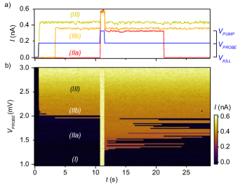
FIG. 3: a) Sequence of bias voltages $V_{\text{SD}}$ applied (blue) and observed current during the protocol for $V_{\text{PROBE}}=1.6$ mV (IIa), $1.98$ mV (IIb), and $2.5$ mV (III), selected from panel b). The device is in the single-dot configuration (see Fig. 1(a)). $V_{\text{SD}}$ is initially set to $V_{\text{KILL}}=0$ mV to start the protocol with the CNT at rest. Then $V_{\text{SD}}$ is increased up to $V_{\text{PROBE}}$ for a given time. self-oscillations are pumped by setting $V_{\text{SD}}$ to $V_{\text{PUMP}}=3$ mV. Finally, the persistence of the self-oscillations is measured by setting $V_{\text{SD}}$ back to $V_{\text{PROBE}}$. b) Observed current during the protocol for different values of $V_{\text{PROBE}}$. We identify four regions: (I) absence of self-oscillations; (IIa) self-oscillations observed after the pumping step and spontaneously decaying after a random time; (IIb) self-oscillations spontaneously appearing at a bias potential $V_{\text{SD}}=V_{\text{PROBE}}$; and (III) stable self-oscillations.

Fig. 3(b) summarizes our experimental results for a wide range of $V_{\text{PROBE}}$. We identify four different regimes associated with the three regions in Fig. 2. For $0<V_{\text{PROBE}}<1.5$ mV, region (I), the absence of current indicates that self-oscillations are not stable. They do not appear spontaneously at $V_{\text{SD}}=V_{\text{PROBE}}$ and vanish immediately after the pumping step. In region (IIa), $1.5\,\,\mbox{mV}<V_{\text{PROBE}}<2.0$ mV, self-oscillations do not start spontaneously but endure during a random time after being triggered by the pumping step. In a small bias voltage range around $V_{\text{PROBE}}\approx 2.0$ mV, region labeled as (IIb), self-oscillations can start spontaneously after some time at $V_{\text{PROBE}}$. Finally, for $V_{\text{PROBE}}>2\leavevmode\nobreak\ \text{mV}$, region (III), self-oscillations are always stable: they start spontaneously at $V_{\text{PROBE}}$ and are maintained during the whole protocol.

In the bistable regions, (IIa) and (IIb), self-oscillations appear and vanish due to fluctuations that allow the system to access areas in the stability diagram of Fig. 2(b) that have the opposite sign of $\Delta E$ than that dictated by our deterministic model. The probability of these excursions is very small but can occur after a large number of oscillations. For instance, a self-oscillation of frequency $\Omega/2\pi\sim 270$ MHz can last for 20 seconds or $5.4\times 10^{9}$ oscillations. This mechanism explains the huge separation of time scales in the device. One can identify two main sources of fluctuations: the thermal noise affecting the motion of the nanotube and quantum noise due to tunneling. The latter is much larger than the former, but is present only when a current flows through the CNT. This explains why fluctuations are more likely to terminate rather than to induce self-oscillations, as observed in Fig. 3(b).

We perform a similar study when the device is in the double-dot configuration by measuring the hysteresis as a function of $V_{\text{SD}}$ (Fig. 4(a)) at the point designated by the white star in Fig. 1(d). The sharp changes in current are reproducible over several sweeps of $V_{\text{SD}}$ for a different thermal cycle of the device (see Supplemental Material [46]), with a small variation in threshold voltages due to the stochastic nature of this process. In the double dot configuration, the hysteretic switches define regions (i) to (iv). In region (iii) we observe current values evidencing self-oscillations, while in regions (i) and (v) these self-oscillations seem not to be present.

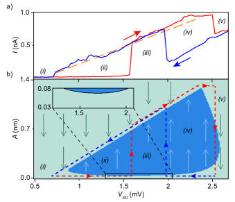
FIG. 4: a) Current switch hysteresis as function of $V_{\text{SD}}$ in the double-dot configuration, measured at the white star location in Fig. 1(d) ($V_{\text{G3}}=620$ mV, $V_{\text{G5}}=-120$ mV). Red and blue arrows indicate the direction of each current sweep. The dashed orange line shows the current calculated from Eq. (5) with $\Gamma_{\rm M}=\Omega$, $\sigma=0.1$ nm and amplitude 1 nm (see Supplemental Material [46] for details). The numerals (i, ii, iii, iv, v) indicate different regions in the stability diagram. b) Stability diagram: the dark (light) blue areas indicate $\Delta E>0$ $(\Delta E<0)$ for different values of A and $V_{\text{SD}}$. Small arrows indicate the direction in which A would change in each area given the sign of $\Delta E$. Blue an red dashed lines delimit regions (ii), (iii) and (iv). Blue and red arrows indicate a similar hysteresis cycle as that shown in panel a). Inset: zoom in on areas approaching zero amplitude. We use $\Omega/2\pi=270$ MHz, $g_{\rm m}=0.01$ eV$/$nm, $m=2\times 10^{-22}$ kg, and $Q=1000$.

These current switches can be explained by our model under the assumption that the motion of the CNT mostly affects the electrochemical potential of one of the dots. This assumption is justified by the estimation of capacitive coupling of the quantum dots to the gate electrodes which indicates that one of the dots is primarily controlled by $V_{\text{G3}}$, whilst the other is mainly controlled by $V_{\text{G5}}$. The electrochemical potential of the second dot can thus be considered approximately aligned with $\mu_{\text{D}}=0$. In this case, the system is similar to the one-dot case but replacing the transport between the dot and the rightmost electrode by tunneling between the two dots occurring when their electrochemical potentials are aligned, i.e., when $x(t)$ is close to zero; in the model, this interdot exchange is represented by the rate $\Gamma_{\rm M}$ and a width $\sigma$ (see Supplemental Material [46]). However, notice that, contrary to the case of a single dot, self-oscillations disappear for high bias voltages $V_{\text{SD}}$ (region (v)). Indeed, this phenomenon is difficult to explain with the model outlined above, since $V_{\text{SD}}$ simply determines the location of the leftmost Fermi level $\mu_{\text{S}}$ and should not affect the stability of self-oscillations. Notice, however, in Eq. (4), that self-oscillations are maintained by a correlation between the charge of the dot $n(t)$ and the instant velocity of the CNT, $v(t)$. This correlation could be lost due, for instance, to inelastic co-tunneling , which is present for high values of $V_{\text{SD}}$ (see Supplemental Material [46]).

For the double-dot case, which now considers interdot tunneling and an inelastic contribution to the current proportional to $V_{\text{SD}}$ [46], we obtain the current shown in Fig. 4(a) (orange line) and the stability diagram depicted in Fig. 4(b). The stability diagram shows good agreement with the measured current switches as a function of $V_{\text{SD}}$ in upwards (red) and downwards (blue) sweeps, although the boundaries of region (iii) are not precisely located due to its stochastic nature. We can also observe that the area with $\Delta E<0$ (light blue) appears close to zero $A$ in region (iii) (see also the inset). This would indicate that the rest position of the CNT is unstable and self-oscillations can be easily induced by fluctuations, a picture which is supported by the measurements of the onset of self-oscillations in region (iii) (see Supplemental Material [46]).

In conclusion, we were able to construct stability diagrams that fully characterize the oscillations induced by electron tunneling in single and double quantum dot configurations. We achieve this by observing hysteresis cycles in the current flowing through the device, by using a novel protocol to probe, pump and kill these self-oscillations, and by developing a dynamical model. Our results reveal the subtleties in the coupling between mechanical motion and single electron transport, and open new venues to design autonomous motors and other types of energy transducers at the microscale.

Supplemental Material

.1 Decay of self-oscillation

The switching between states in the bistability region finds its origin in the thermal and electric noise. In order to clarify this, we expose the bistability in terms of the well known double-well problem [47, 19, 20] in the single-dot configuration. We now consider a long time scale $T_{A}\gg 1/\Gamma$ where the amplitude of oscillation will vary with time. In this time scale, we consider an effective Langevin equation for the mechanical energy,

$$\frac{dE}{dt}=f(E)+\xi_{E},$$ (1)

where $f(E)=\Delta E/\tau$, is the average increment of energy per unit of time. $\tau=2\pi/\Omega$ is the period of the oscillation. $\xi_{E}$ is a noise containing both electrical and thermal fluctuations, and will depend on the actual value of energy.

This equation can be written as a Kramers equation considering an effective ”potential” given by

$$U(E)=-\frac{1}{\tau}\int_{0}^{E}\Delta E(E^{\prime})dE^{\prime},$$ (2)

then,

$$\frac{dE}{dt}=-\frac{dU}{dE}+\xi_{E}.$$ (3)

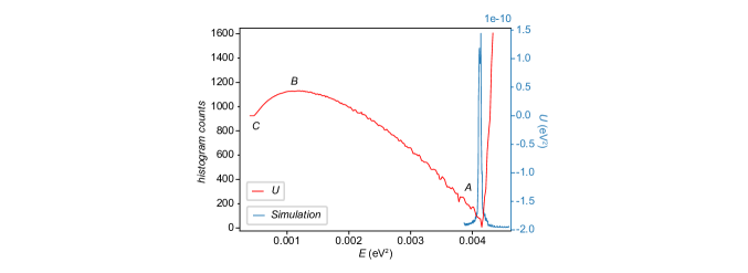
FIG. S1: Numerical computation of the effective potential $U(E)$ (red) stochastic simulation of a single trajectory (blue) as a function of the mechanical energy for the one dot-configuration. The sharp peak in $U$ at the point A is due to the end of the borders of the conduction region of the device. Letters A, B, C indicate the stable oscillation points of the oscillation (A, C) and the tipping point between both regimes (B).

The effective potential is represented in Fig. S1 (red line). Here, the problem is explicitly analog to the typical double well potential, in energy space and a coloured noise. In that figure, self-oscillations correspond to the right well, A, with a certain energy associated. The other well, C, corresponds with the motionless state. Switching between both states will happen when a fluctuation puts the system over the barrier B.

We simulate one trajectory in the self-oscillation state for $10^{4}$ oscillation periods, and included their histogram in Fig. S1 (blue). This histogram is sharply peaked in the the point A, suggesting the appearance of an Arrhenius law in self-oscillation during time.

.2 Double-dot model

As exposed in the main text, the gate voltages inducing the configurations are $V_{\text{G3}}$ and $V_{\text{G5}}$, and then one of the dots is located close to the center of the CNT and can moves as in the single-dot configuration, whereas the second one is close to the rightmost end of the CNT, remaining static. This system is similar to the one-dot case but replacing the transport between the moving dot and the right lead by an effective tunneling rate with the form $\Gamma_{\rm dot-dot}(x)=\Gamma_{\text{M}}\exp{-x^{2}/\sigma^{2}}$. The width $\sigma$ represents the effects of the thermal noise on the moving dot.

However, notice that, contrary to the case of a single dot, self-oscillations disappear for high bias voltages $V_{\text{SD}}$, see main text. This happens as a result of the inelastic current, promoting transport even between misaligned dots [41, 48]. In (iii, iv, v) we will calculate inelastic transport in a completely effective way, including homogeneous transport rates $\Gamma^{\rm ie}(V_{\text{SD}})$ in the master equation,

$$\Gamma_{\rm in}(x) =\Gamma_{\text{L}}(x)f_{\text{L}}(\epsilon(x))+\Gamma^{\rm ie}(V_{\text{SD}})$$ (4)

$$\Gamma_{\rm out}(x) =\Gamma_{\text{L}}(x)[1-f_{\text{L}}(\epsilon(x))]+\Gamma_{\rm dot-dot}(x)+\Gamma^{\rm ie}(V_{\text{SD}}),$$ (5)

and obtaining their value from the motionless state. In regions (i, ii) we state $\Gamma^{\rm ie}(V_{\text{SD}})=0$ for every $V_{\text{SD}}$.

.3 Double-dot statistics

For the double-dot configuration, we have implemented a similar protocol as for the single dot configuration in Fig. 3 of the main text (Fig. S2(a)). The measurement is performed at the coordinates of the white star in Fig. 1e of the main text, in the same configuration as in Fig. 4 of the main text. The pump voltage $V_{\text{PUMP}}=1.8$ mV is chosen the area were the self-oscillations are always on (Fig. S2(b)).

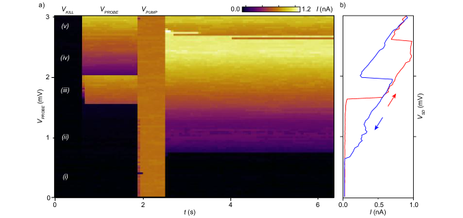
FIG. S2: a) Voltage bias sequence applied to measure panel b). First any SO are killed setting $V_{\text{SD}}$ to $V_{\text{KILL}}=0$ mV, then $V_{\text{SD}}$ is set to the target voltage $V_{\text{PROBE}}$. About 1.5 s later, $V_{\text{SD}}$ is set to $V_{\text{PUMP}}=1.8$ mV to start SO for about 0.5 s. Finally, the voltage is set back to the target $V_{\text{SD}}$. b) Current measured by repeating the sequence shown in panel a) for different $V_{\text{PROBE}}$. The different behaviors are classified in five areas: (i) absence of self-oscillations, (ii) self-oscillations observed after the pumping step, (iii) self-oscillations spontaneously appearing, (iv) self-oscillations observed after the pumping step and spontaneously decaying after a random time, (v) absence of self-oscillations. c) IV measurement with the two sweep direction in the configuration of panel b) showing the current switch hysteresis; same as Fig. 4(a) of the main text.

From the current measurement, depicted in Fig. S2(b), we identify different behaviors depending on $V_{\text{SD}}$. In (i) and (ii), self-oscillations never start spontaneously, whereas in (iii) they start spontaneously just after the kill step. After the pump step, in regions (i) and (v) self-oscillations stop immediately. In regions (ii) and (iv) the triggered self-oscillations are sustained for a duration too long to be observed in the time frame of this experiment. In the border between regions (iv) and (v) the self-oscillations time decays in a similar way as observed in the single-dot configuration.

.4 Fitting of the Coulomb peak and tunneling rates

We fit the coulomb diamond in the single dot configuration to estimate the tunneling rates parameters $\Gamma_{\text{L,R}}$ and $\alpha_{\text{L,R}}$. The fitting procedure is similar to our previous work [14] with the addition of energy-dependent tunneling rates, represented by the parameter $\alpha_{\text{L,R}}$, inspired from Ref. 12. The rates of charges tunneling in and out between the left (L) or right (R) lead and the quantum dot are given by the expression:

$$\Gamma_{\text{L,R}}^{\text{in}}(\epsilon)=\Gamma_{\text{L,R}}\exp(\alpha_{\text{L,R}}\epsilon/g_{\rm m})\leavevmode\nobreak\ \rho_{\text{L,R}}(\epsilon),$$ (6a)

$$\Gamma_{\text{L,R}}^{\text{out}}(\epsilon)=\Gamma_{\text{L,R}}\exp(\alpha_{\text{L,R}}\epsilon/g_{\rm m})\left(1-\rho_{\text{L,R}}(\epsilon)\right),$$ (6b)

where, as in the main text, $\epsilon$ is the energy of the dot and $f_{\text{L,R}}$ are the Fermi distribution. The the overlap between the density of states of the quantum dot and left/right reservoirs is given by:

$$\rho_{\text{L,R}}(\epsilon)=\frac{1}{2}+\frac{1}{\pi}\arctan\left(\frac{2(\upmu_{\text{L,R}}-\epsilon)}{\hbar\Gamma_{\text{tot}}}\right).$$ (7)

Finally the current across the quantum dot is:

$$I(\epsilon)=e\frac{\Gamma_{\text{L}}^{\text{in}}(\epsilon)\Gamma_{\text{R}}^{\text{out}}(\epsilon)-\Gamma_{\text{R}}^{\text{in}}(\epsilon)\Gamma_{\text{L}}^{\text{out}}(\epsilon)}{\Gamma_{\text{tot}}}.$$ (8)

We fit the experimental the coulomb diamonds in Fig. S3(a) by cutting it into multiple coulomb peak with bias ranging from $V_{\text{SD}}=0$ mV to $V_{\text{SD}}=0.9$ mV (Fig. S3(b)). We fit these coulomb peaks with a unique set of parameters to obtain $\Gamma_{\text{L}}$ = 400 GHz, $\Gamma_{\text{R}}$= 15 GHz, $\alpha_{\text{L}}=0\leavevmode\nobreak\ \text{eV}^{-1}$ and $\alpha_{\text{R}}=400\leavevmode\nobreak\ \text{eV}^{-1}$.

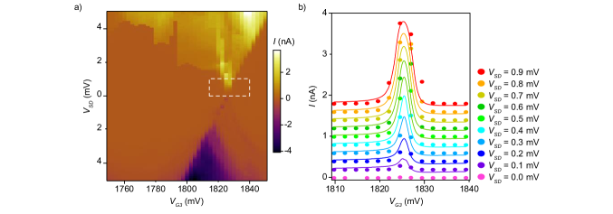
FIG. S3: Coulomb diamond and fit. a) Zoom on the coulomb diamond from Fig. 1d of the main text. The white dashed rectangle represent the area from which are obtain the cut of panel b). b) Set of cuts of panel a) at different bias (circles) and fitting curves (lines). For each bias, the cuts and fit are vertically offset by 0.2 nA from the previous bias. The fitting parameters of the all set are: $\Gamma_{\text{L}}$ = 400 GHz, $\Gamma_{\text{R}}$= 15 GHz, $\alpha_{\text{L}}/g=0\leavevmode\nobreak\ \text{eV}^{-1}$, $\alpha_{\text{R}}/g=400\leavevmode\nobreak\ \text{eV}^{-1}$ and $V_{0}=1.826$ V. The lever arm 0.18 eV/V is obtain from panel a).

To take into consideration the voltage drop at the IV converter internal resistance (100 k$\Omega$), we reduce the bias of the fit by $V_{\text{SD}}^{\text{Corr}}(V_{\mathrm{G1}})=V_{\text{SD}}-I(V_{\mathrm{G3}})R_{\mathrm{s}}$. Because the density of point of the measurement is not sufficient we calculate $V_{\text{SD}}^{\text{Corr}}$ from a first fit of the coulomb peaks. We then fit again the peaks considering the corrected bias voltage. The contribution of this correction on the final result is small.

.5 Stability diagram

Here we show a large measurement of the stability diagram of the carbon nanotube going from the single dot to the double dot configurations.

FIG. S4: Stability diagram containing the single quantum dot and double quantum dot regime measured at $V_{\text{SD}}=3$ mV.

.6 Additional results

Here we present additional results obtain with the same device but during a different cool down. The device have been endure a thermocycle at 300 K between the results shown in the main text and the one presented in the following.

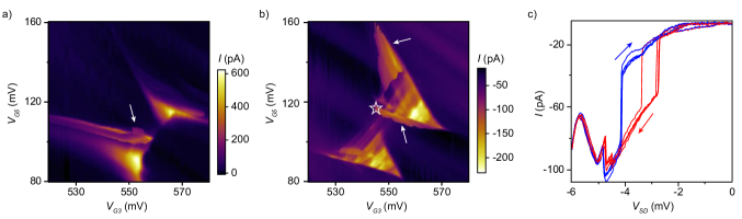
FIG. S5: Results obtained on the same device but during a different cool down than the results presented in the main text. a,b) Bias triangles measured on the double quantum dot regime for $V_{\text{SD}}=4$ mV (a) and $V_{\text{SD}}=-4$ mV. SO are visible in the edge of one of the triangles highlighted by the arrow. c) SO hysteresis measured as at the position of the white star in panel b). 5 sweeps, back and forth, was repeated. The arrows indicate the direction of the sweep.

In Fig. S5(a) and Fig. S5(b) we show the measurement of a bias triangle with positive and negative bias voltage ($V_{\text{SD}}=\pm 4$ mV) showing that the device is in the double quantum dot configuration. Evidence of self-oscillation are visible one particular edge of one of the triangle in both bias polarity. This edge correspond to the chemical potential of one of the two dots (the same in both polarity) align with the chemical potential of the contact lead of its side [41].

We measure the hysteresis of the self-oscillation (Fig. S5(c)) at coordinates of the white start in Fig. S5(b), located in the edge of the self-oscillation area. The hysteresis is measured multiple time in a row and show a bistability region from $V_{\text{SD}}=-4$ mV to $V_{\text{SD}}=-2$ mV.

.7 Mechanical excitation of the self-oscillations

To evidence the mechanical nature of the current switch that we associate to self-oscillation we use a radio-frequency tone normally used to drive the carbon nanotube into motion to trigger the self-oscillation. This is highlighted by the results shown in Fig. S6, obtained during both cool down.

FIG. S6: Measurement of radio-frequency triggering of the SO performed at the position of Fig. S2(b) (a), $V_{\text{SD}}=0.6$ mV, and at the white star in Fig. S5(b) (b) for a bias of $V_{\text{SD}}=-3$ mV. The current is measured under radio-frequency excitation at frequency $\omega_{\mathrm{drive}}$ close to the mechanical resonance frequency $\Omega$ as function of the excitation power $P_{\mathrm{drive}}$. In panel b), for each pixel, $V_{\text{SD}}$ was set to 0 mV for 0.1 s, to kill any residues self-oscillation, then set back to $-3$ mV for the measurement while a continuous radio-frequency excitation.

We apply a driving rf tone to the carbon nanotube, near the mechanical resonance frequency, while the device is in the bistability region. The result evidences a triggering of the self-oscillation at low drive power $P_{\mathrm{drive}}$ when the frequency of the tone $\omega_{\mathrm{drive}}$ equal the fundamental mechanical resonance frequency $\Omega$. Note that mechanical resonance frequency slightly changed between the two cool down. This demonstrate the mechanical pumping of the self-oscillations in the bistability region. In particular in Fig. S6(b) the bias is initially set to $V_{\text{SD}}=0$ mV for 0.1 s to kill any self-oscillations then set back to $V_{\text{SD}}=-3$ mV for an other 0.1 s when the current is measured. Most of the time, the self-oscillations consistently restart with the drive, near the mechanical resonance frequency. The self-oscillations start in a much broader frequency range at high power probably due to the effective gate voltage change induced by the radio-frequency drive.