(a) The initial state

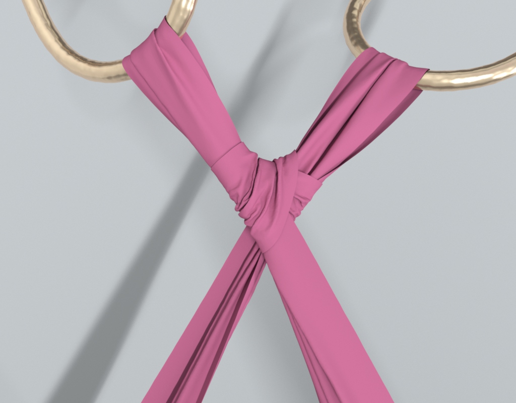
(b) The tightening state

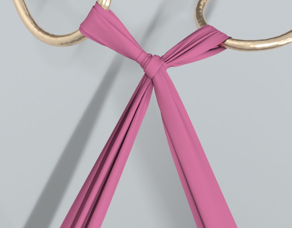
(c) The final state

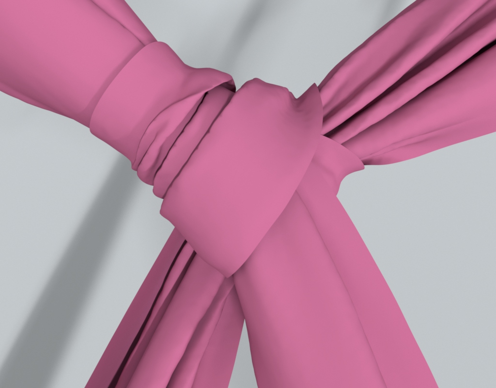
(d) The final state in a closeup

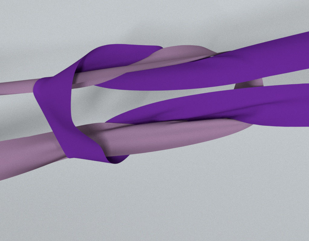
(e) The initial state

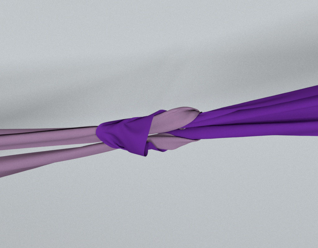
(f) The tightening state

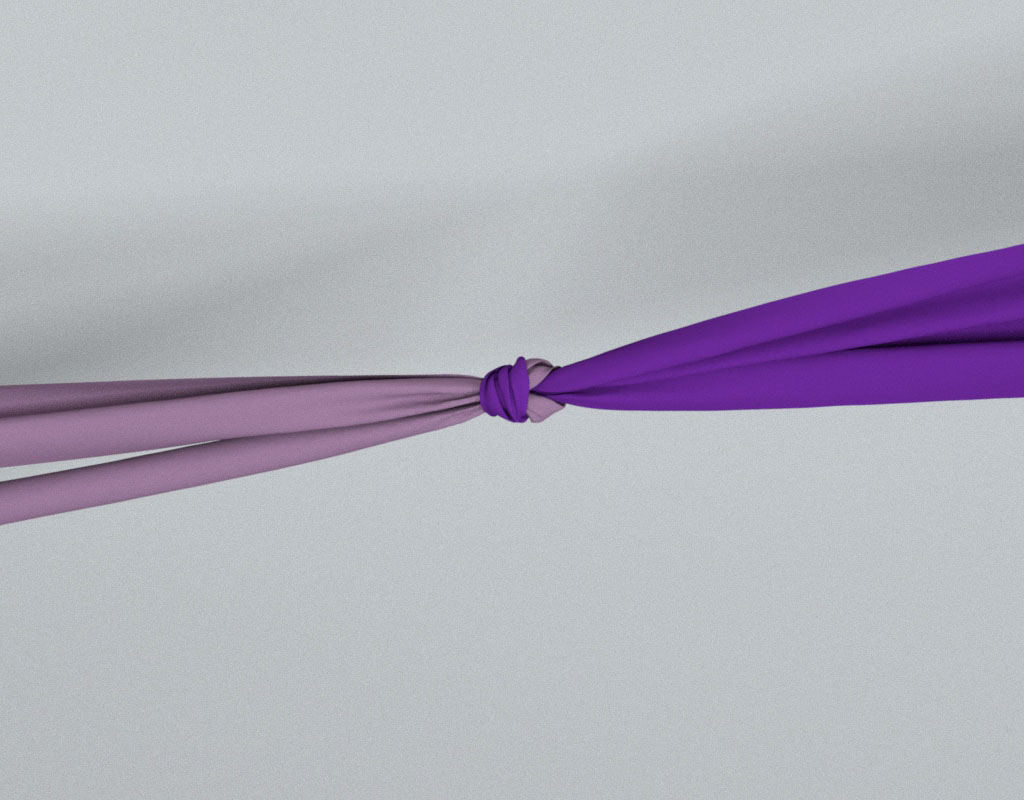
(g) The final state

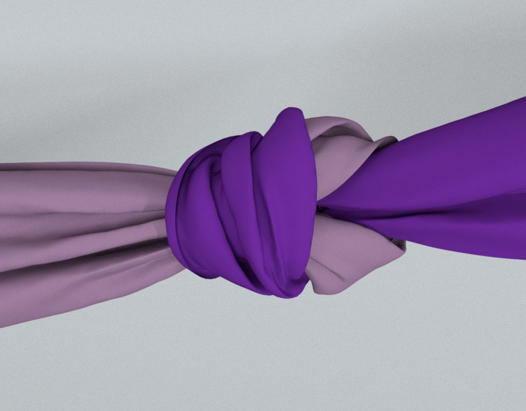
(h) The final state in a closeup

Figure 1. Knotting. The bow knot example (on the top, with 142K triangles) and the reef knot example (on the bottom, with 71K triangles) are presented. In this work, we develop a two-way method for safe and fast collision handling in deformable body simulation. Thanks to this method, our simulator can robustly handle complex collision contacts in these two examples at 4 to 17 FPS and 10 to 21 FPS.

Fast GPU-Based Two-Way Continuous Collision Handling

Abstract.

Step-and-project is a popular way to simulate non-penetrated deformable bodies in physically-based animation. First integrating the system in time regardless of contacts and post resolving potential intersections practically strike a good balance between plausibility and efficiency. However, existing methods could be defective and unsafe when the time step is large, taking risks of failures or demands of repetitive collision testing and resolving that severely degrade performance. In this paper, we propose a novel two-way method for fast and reliable continuous collision handling. Our method launches the optimization at both ends of the intermediate time-integrated state and the previous intersection-free state, progressively generating a piecewise-linear path and finally reaching a feasible solution for the next time step. Technically, our method interleaves between a forward step and a backward step at a low cost, until the result is conditionally converged. Due to a set of unified volume-based contact constraints, our method can flexibly and reliably handle a variety of codimensional deformable bodies, including volumetric bodies, cloth, hair and sand. The experiments show that our method is safe, robust, physically faithful and numerically efficient, especially suitable for large deformations or large time steps.

1. Introduction

The simulation of intersection-free deformable body dynamics can be formulated as a constrained optimization problem (Kane et al., 1999; Martin et al., 2011):

(1) $$\mathbf{x}^{t+1}=\mathop{\arg\min}\limits_{\mathbf{x}}{E\big{(}\mathbf{x},\mathbf{x}^{t},\mathbf{v}^{t}\big{)}},\quad\;\mathrm{s.t.}\;\;\mathcal{X}\big{(}\mathbf{x}^{t},\mathbf{x}\big{)}\subset\Omega,$$

in which $\mathbf{x}^{t},\mathbf{v}^{t}\in\mathbb{R}^{3N}$ are the stacked position and velocity vectors of $N$ vertices at time $t$, $E(\mathbf{x},\mathbf{x}^{t},\mathbf{v}^{t})$ is the dynamics objective, $\mathcal{X}(\mathbf{x}^{t},\mathbf{x})$ is a sufficiently short linear or piecewise linear path from $\mathbf{x}^{t}$ to $\mathbf{x}$, and $\Omega$ is the feasible intersection-free region. Li et al. (2020a; 2021) showed that augmenting the objective function with a smoothed Log-barrier-based contact energy term to convert the original constrained problem into an unconstrained one and then using Newton’s method with a continuous-collision-detection-based pre-filtered line search strategy (Smith and Schaefer, 2015) could get globally convergent solutions.

However, their techniques are computationally expensive, due to the frequent launching of the high cost dynamics solver and truncated step sizes needed for keeping the path within $\Omega$. A common strategy (Harmon et al., 2008; Narain et al., 2012; Tang et al., 2016, 2018b, 2018a; Li et al., 2020b) for more efficient simulation is to divide the optimization into two steps:

(2) $$\left\{\begin{array}[]{l}\mathbf{y}^{[k+1]}=\mathop{\arg\min}\limits_{\mathbf{y}}Q_{k}\big{(}\mathbf{y},\mathbf{x}^{[k]},\mathbf{x}^{t},\mathbf{v}^{t}\big{)},\\ \mathbf{x}^{[k+1]}=\mathop{\arg\min}\limits_{\mathbf{x}}{D\big{(}\mathbf{x},\mathbf{y}^{[k+1]}\big{)}},\quad\;\mathrm{s.t.}\;\;\mathcal{X}\big{(}\mathbf{x}^{[k]},\mathbf{x}\big{)}\subset\Omega.\end{array}\right.$$

In each iteration, firstly the dynamics solver forms a quadratic model $Q_{k}$ (or a linear model $L_{k}$ (Wang and Yang, 2016; Wu et al., 2020)) of $E(\mathbf{x},\mathbf{x}^{t},\mathbf{v}^{t})$ at $\mathbf{x}^{[k]}\in\Omega$ to compute a target state $\mathbf{y}^{[k+1]}$, and then a collision handling module addresses all potential intersections to obtain a feasible state $\mathbf{x}^{[k+1]}$. Here $D(\mathbf{x},\mathbf{y}^{[k+1]})$ is a metric measuring the distance between $\mathbf{x}$ and $\mathbf{y}^{[k+1]}$, which is supposed to be significantly simpler than $E(\mathbf{x},\mathbf{x}^{t},\mathbf{v}^{t})$. After several iterations of Eq. (2), the algorithm reports $\mathbf{x}^{[k+1]}$ as $\mathbf{x}^{t+1}$ for Eq. (1). This strategy avoids frequent launching of high-cost solvers such as (Li et al., 2020a; Li et al., 2021), but it sacrifices part of accuracy in exchange for performance since this alternating approach might not converge to a local minimum. Li et al. (2021) showed that this inaccuracy could be observed from the wrinkling or jittering artifacts and parameter tuning could alleviate this problem.

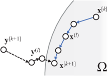
Figure 2. The two-way collision handling approach.

Intuitively, the collision handling module projects $\mathbf{y}^{[k+1]}$ back to $\Omega$, but it also needs to ensure that a sufficiently short path exists to avoid tunneling artifacts as shown in Fig. 4(a). In the past, researchers (Harmon et al., 2008; Narain et al., 2012; Tang et al., 2016, 2018b, 2018a; Li et al., 2020b) parameterized this path as a line segment and evaluated $\mathcal{X}(\mathbf{x}^{[k]},\mathbf{x})\subset\Omega$ by continuous collision detection (CCD) tests. This solution is generally plausible when $\mathbf{y}^{[k+1]}$ is close to $\mathbf{x}^{[k]}$, but it is no longer the case as two states go far away from each other, where finding $\mathbf{x}^{[k+1]}$ on the line segment that passes all of the CCD tests can become extremely difficult (Tang et al., 2018b). Besides, how to measure the distance for projection is also crucial for realistic simulation. Using mass-weighted $L_{2}$ norm is straightforward for a minimal change in post-response kinetic energy (Harmon et al., 2008; Narain et al., 2012; Tang et al., 2016, 2018b, 2018a; Li et al., 2020b), but it can severely distort local elements to resolve all contacts (see Figs. 17 and 18), resulting in spuriously over-stretched artifacts or oscillations over time.

In this paper, we develop a collision handling algorithm for the step-and-project method, capable of finding a quality solution $\mathbf{x}^{[k+1]}$ at a low cost. Our key idea is a two-way approach shown in Fig. 2. In this approach, we iteratively solve two steps: a backward step finding a sequence of targets $\{\mathbf{y}^{(l)}\}$ by impact zone optimization as a guidance for the evolution of $\mathbf{x}$, and a forward step generating the actual path $\mathcal{X}(\mathbf{x}^{[k]},\mathbf{x})\subset\Omega$ by conservative vertex advancement towards the guidance. As the forward step finds a sequence of states $\{\mathbf{x}^{(l)}\}$, satisfying $(1-t)\mathbf{x}^{(l)}+t\mathbf{x}^{(l+1)}\in\Omega$ for any $t\!\in\![0,1]$ and $l$, we essentially form $\mathcal{X}(\mathbf{x}^{[k]},\mathbf{x})$ as a piecewise linear path rather than linear ones (Harmon et al., 2008; Narain et al., 2012; Tang et al., 2016, 2018b, 2018a; Li et al., 2020b) by relaxing the restriction on the searching space. Aiming at both efficiency and quality for resolving contacts, we make the following technical contributions.

• An inexact backward step.     We formulate impact zone optimization as a linear complementary problem and solve it inexactly by a small number of iterations in each backward step. In addition, we introduce soft unilateral constraints on edge length to effectively eliminate oscillations caused by large local element deformations.

• A lightweight forward step.     Instead of using CCD tests, we use fast discrete distance evaluation to calculate safe asynchronous step sizes, which enables to keep the path generated in each forward step safely staying inside $\Omega$.

We show that our two-way collision handling algorithm can be conveniently implemented on a GPU and integrated into our in-house GPU-based deformable body simulator. Coupled with volume-based contact constraints, our simulator is capable of simulating a variety of codimensional examples (see Figs. 1 and 3), including volumetric bodies, cloth, hair and sand. The experiments show our system is safe, fast, GPU-friendly, and robust against large time steps and deformations.

2. Related Work

Discrete collision handling.

Researchers (Baraff et al., 2003; Volino and Magnenat-Thalmann, 2006; Wicke et al., 2006) developed discrete collision handling methods to remove intersections at the end of every time step. If a discrete collision handling method fails to eliminate all of the intersections, it can still repeat the process in the next time step, hopefully achieving the intersection-free state later. Therefore a discrete collision handling method is robust regardless of the time step. But as the time step increases, it becomes less likely to remove all of the intersections, which leads to long-lasting penetration artifacts in simulation.

Many physics-based simulators apply repulsion forces among proximity pairs to lessen the likelihood of collisions. Broadly speaking, this repulsion approach is a discrete collision handling method, as it calculates repulsive forces based on proximity distances discretely evaluated in time. Thanks to its simplicity, the repulsion approach is widely used in GPU-based simulation (Stam, 2009; Fratarcangeli et al., 2016; Wang and Yang, 2016) alone, without support from any other method. To help the repulsion approach achieve intersection-free guarantee, Wu et al. (2020) presented a fail-safe Log-barrier repulsion phase, whose usage should be minimized due to a large computational overhead.

Continuous collision handling.

The main difference between discrete collision handling and continuous collision handling is that discrete collision handling tries to eliminate intersections at the end of the time step, while continuous collision handling must resolve all of the intersections at any time. A typical continuous collision handling method contains two components: continuous collision detection (CCD) and applying collision responses. Continuous detection of a vertex-triangle or edge-edge collision involves solving a cubic equation, which could be prone to errors (Provot, 1997; Ainsley et al., 2012; Wang, 2014; Tang et al., 2014), especially in the single-precision floating-point computation environment. Recently, Yuksel (2022) presented an efficient and robust method for finding real roots of cubic and higher-order polynomials and Lan et al. (2022) provided a re-designment of the CCD root finding procedure on GPU. For the robustness of CCD queries, we recommend (Wang et al., 2021) for a more detailed discussion. In addition to the possible robustness issue, the typical spatial acceleration structures used for CCD, such as bounding volume hierarchies (BVHs) and bounding volume traversal trees (BVTTs), could be hard to parallelize (Tang et al., 2011a, 2016).

But compared with CCD, obtaining the right collision responses is an even greater challenge. Bridson et al. (2002; 2005) initially used geometric impulses as responses and the rigid impact zone technique as a failsafe. To avoid the locking artifacts caused by the rigid impact zone technique, Harmon et al. (2008) calculated collision responses by non-rigid impact zone optimization. ARCSim (Narain et al., 2012) used this method as its inner collision handling component and provided an open-sourced implementation based a combination of BVH-based CCD and an augmented Lagrangian solver for collision response. CAMA (Tang et al., 2016), PSCC (Tang et al., 2018a), I-Cloth (Tang et al., 2018b), and P-Cloth (Li et al., 2020b) further improved its performance on GPU(s) in two aspects.

• Faster CCD on GPU(s).     In detail, this benefits from localized BVTT front propagation exploiting spatio-temporal coherence (Tang et al., 2016), parallel normal cone culling with spatial hashing (Tang et al., 2018a), incremental collision detection with spatial hashing exploiting spatio-temporal coherence (Tang et al., 2018b), and distributing the incremental collision detection on multiple GPUs (Li et al., 2020b).

• More GPU-friendly non-rigid impact zone solver.     In detail, this benefits from assembling all of the impacts into one linear system to perform inelastic projection (Tang et al., 2016), paralleling the augmented Lagrangian method of ARCSim in a gradient-descent manner (Tang et al., 2018b), and further paralleling the augmented Lagrangian method on multiple GPUs (Li et al., 2020b).

We note that although the performance is continuously improved in these step-and-project methods, both the assumption of linear paths and simply measuring the projection distance via mass-weighted $L_{2}$ norm are inherited, and even the specific choice of the augmented Lagrangian method for collision response is inherited in (Narain et al., 2012; Tang et al., 2018b; Li et al., 2020b).

Recently, Log-barrier-based methods (Wu et al., 2020; Li et al., 2020a; Li et al., 2021) have emerged to be popular choices for collision handling in physical animation. They usually employ a smoothed (Li et al., 2020a; Li et al., 2021) or unsmoothed (Wu et al., 2020) Log-barrier potential term to augment the objective, so that the potential term could be extremely large to “push” against the boundary of the feasible region. However, it is not enough for guaranteeing the state stays in the feasible region and they usually employ CCD to compute an upper bound of the safe distance to make sure no intersection happens. Clearly, the strength of these methods is its safety, but notoriously slow for two reasons.

• Frequent tests.     The method needs to repetitively test the vertices in every optimization step, to make sure that no intersection occurs.

• Barrier functions.     Barrier functions push $\mathbf{x}$ sufficiently against the feasible region boundary $\partial\Omega$, only when $\mathbf{x}$ gets close to $\partial\Omega$.

We note that many continuous collision handling methods may require considerable implementation efforts to get accelerated on GPUs (Tang et al., 2016, 2018a; Lauterbach et al., 2010; Li et al., 2020b), due to their high dependency on sequential tasks (Li et al., 2021) and high complexity (Tang et al., 2018b).

Asynchronous steppings.

The conservative advancement approach (Mirtich and Canny, 1995; Von Herzen et al., 1990) for rigid body collision handling suffers from the small stepping issue, as it requires all of the bodies to take the same step size. Mirtich (2000) addressed this issue by allowing rigid bodies to take different step sizes, while still respecting causality. Researchers (Thomaszewski et al., 2008; Harmon et al., 2009) later investigated this idea for asynchronous collision handling of cloth, and explored several speedup options (Harmon et al., 2011; Ainsley et al., 2012). Our method is also asynchronous: vertices away from collisions can take large step sizes to reach their targets fast. More importantly, it avoids CCD tests and it is naturally free of performance or robustness issues associated with them.

Broad-phase collision culling.

Broad-phase collision culling is important to collision handling methods, as it avoids unnecessary collision tests for collision-free primitive pairs. In general, collision culling techniques fall into two categories: those based on BVHs (Lauterbach et al., 2010; Wang et al., 2017; Tang et al., 2011b, 2010) and those based on spatial hashing (Teschner et al., 2003; Pabst et al., 2010; Zheng and James, 2012; Barbič and James, 2010; Tang et al., 2018a). While GPU implementations of both categories have been investigated before, GPU-based spatial hashing is arguably more popular, thanks to its simplicity and parallelizability. Our method is orthogonal to collision culling techniques and it can adopt more advanced ones later.

Frictional contacts

How to simulate frictional contacts, especially frictional self contacts, is another challenging problem in deformable body simulation. The popular velocity filtering approach (Bridson et al., 2002; Müller, 2008) is simple, fast, but not so physically plausible, as it handles collisions and frictions in separate processes. Recently, researchers (Daviet, 2020; Verschoor and Jalba, 2019; Bertails-Descoubes et al., 2011; Macklin et al., 2019; Ly et al., 2020; Li et al., 2020a) are interested in handling collisions and frictions together through joint optimization. While our work does not consider friction, we plan to borrow their ideas for simulating plausible frictional contacts in the future.

Input: the current state $\mathbf{x}^{[k]}$, the target state ${\mathbf{y}}^{[k+1]}$,         the proximity search bound $\left[D^{\min},\,D^{\max}\right]$, the step number limit $L$ and the termination condition $\epsilon$.

1 $\mathbf{x}^{(0)}\leftarrow\mathbf{x}^{[k]}$;

2 $\mathbf{y}^{(0)}\leftarrow{\mathbf{y}}^{[k+1]}$;

3 $D^{(0)}\leftarrow 0$;

4 $\mathbf{r}^{(0)}\leftarrow\mathbf{1}$;

5 $\mathcal{P}\leftarrow\emptyset$;

6 for $l=0...L$  do

7      if $D^{(l)}<D^{\min}$ then

8           $\mathcal{P}\leftarrow\mathtt{Proximity\_Search}\big{(}\mathbf{x}^{(l)},\,D^{\max}\big{)}$;

9           $D^{(l)}\leftarrow D^{\max}$;

10          

11           end if

12          $\mathbf{y}^{(l+1)}\leftarrow\mathtt{Backward}\big{(}\mathbf{y}^{(l)},\mathbf{x}^{(l)},\mathbf{y}^{[k+1]},\mathcal{P}\big{)}$  // Sec. 4;

13           $\big{\{}\mathbf{x}^{(l+1)},\mathbf{r}^{(l+1)}\big{\}}\leftarrow\mathtt{Forward}\big{(}\mathbf{x}^{(l)},\mathbf{r}^{(l)},\mathbf{y}^{(l+1)}-\mathbf{x}^{(l)},\mathcal{P}\big{)}$  // Sec. 5;

14          

15          $D^{(l+1)}\leftarrow D^{(l)}-2\max\limits_{i}\big{\|}\mathbf{x}_{i}^{(l+1)}-\mathbf{x}_{i}^{(l)}\big{\|}$;

16           if $\big{\|}\mathbf{r}^{(l+1)}\big{\|}_{\infty}<\epsilon$  then

17                break;

18               

19                end if

20               

21                end for

22               

23               $\mathbf{x}^{[k+1]}\leftarrow\mathbf{x}^{(l+1)}$;

ALGORITHM 1 A two-way method

3. A Two-Way Framework

As we discussed in Section 1, restricting to a linear path and simply taking mass-weighted $L_{2}$ norm as the distance function can be inappropriate for post-projection, especially when $\|\mathbf{y}^{[k+1]}-\mathbf{x}^{[k]}\|$ is large. Thus, we formulate the collision handling as the following optimization problem:

(3a) $$\mathbf{x}^{[k+1]}=\mathop{\arg\min}\limits_{\mathbf{x}}\frac{1}{2}\big{\|}\mathbf{x}-{\mathbf{y}}^{[k+1]}\big{\|}^{2}_{\mathbf{M}},\quad$$

(3d) $$\text{s.t.}\left\{\begin{array}[]{l}\mathcal{X}\big{(}\mathbf{x}^{([k])},\mathbf{x}\big{)}\subset\Omega\\ \mathbf{c}(\mathbf{x},\mathbf{y}^{[k+1]})\geq\mathbf{0},\end{array}\right.$$

in which $\mathbf{M}\in\mathbb{R}^{3N\times 3N}$ is the scaled lumped mass matrix (Tang et al., 2018b). The major differences between our formulation and the ones in (Harmon et al., 2008; Narain et al., 2012; Tang et al., 2016, 2018b, 2018a; Li et al., 2020b) are twofold rooted in Eq. (3d): (i) the path $\mathcal{X}(\mathbf{x}^{([k])},\mathbf{x})$ here should be piecewise linear and sufficiently short, while (Harmon et al., 2008; Narain et al., 2012; Tang et al., 2016, 2018b, 2018a; Li et al., 2020b) restricts it as a linear segment; and (ii) additional edge length constraints $\mathbf{c}(\mathbf{x},\mathbf{y}^{[k+1]})$ are introduced (see Section 4.2 for details) to avoid spuriously large deformations of local elements, which compensates for possible loss of shape preservation by only considering the mass-weighted Euclidean distance. In fact, the projection distance jointly defined by the mass-weighted $L_{2}$ norm plus edge length constraints is more consistently measured as the actual energy, in a sense that we are approximately minimizing the change of both kinetic energy and potential before and after projection. Numerically, such treatment does not complicate the objective function, allowing us to use existing fast iterative techniques as described below.

Our two-way method aims to find a good approximate solution subject to Eq. (3) at a low cost. In this method, two sets of intermediate variables $\{\mathbf{y}^{(l)}\}$ and $\{\mathbf{x}^{(l)}\}$ are introduced and updated alternately in two steps: a backward step starting at $\mathbf{y}^{(0)}=\mathbf{y}^{[k+1]}$, aiming to inexactly and progressively project $\mathbf{y}^{(l)}$ back to $\Omega$ as a target, and a forward step starting at $\mathbf{x}^{(0)}=\mathbf{x}^{[k]}$, aiming to move from the current state $\mathbf{x}^{(l)}\in\Omega$ towards $\mathbf{y}^{(l+1)}$ with a guarantee of $\mathcal{X}(\mathbf{x}^{[k]},\mathbf{x})$ being inside $\Omega$ by conservative vertex advancement. Intuitively, $\{\mathbf{y}^{(l)}\}$ guide the evolution of $\{\mathbf{x}^{(l)}\}$ in the forward step, and in turn $\{\mathbf{x}^{(l)}\}$ explore and update the boundary of the feasible region $\Omega$, which gives feedback to the updates of $\{\mathbf{y}^{(l)}\}$. The supplemental video illustrates our two-way optimization process.

Alg. 1 outlines the pseudo-code of our method: it keeps running the two steps alternately, until the termination metric $\mathbf{r}^{(l+1)}$ is small enough (Algorithm 1) or it reaches the maximum number of iterations $L$ (Algorithm 1). We have $\mathbf{r}^{(l+1)}$ to make sure that the accumulated moving distance from $\mathbf{x}^{[k]}$ to $\mathbf{x}^{(l+1)}$ should be close enough to the distance from $\mathbf{x}^{[k]}$ to $\mathbf{y}^{[k+1]}$. Either way, the method can safely report ${\mathbf{x}}^{(l+1)}$ as its result $\mathbf{x}^{[k+1]}$, no matter if $\mathbf{y}^{(l+1)}$ stays in $\Omega$ or not.

3.1. The Proximity Search

Before diving into details of our method, we first discuss about the proximity search. Functioning as broad-phase collision culling, the proximity search serves multi-fold purposes: to form the set of contact constraints in the backward step (in Subsection 4.1), to obtain proximity pair distances for safe steppings (in Section 5), and to calculate repulsive forces as a part of dynamics (in Subsection 6.2). In our implementation, the proximity search is based on the standard grid-based spatial hashing technique (Pabst et al., 2010; Tang et al., 2018a).

Since the proximity search has non-negligible cost, one challenge is how to reuse the results as often as possible, rather than redoing the search in every step. Let $\mathcal{P}$ be the proximity set in each step that is required to be a superset of all possible pairs whose distances are below a certain bound $D^{\min}$:

(4) $$\mathcal{P}\supset\mathcal{P}_{D^{\min}}=\{\mathcal{p}\mid\forall\mathcal{p}:\mathtt{dist}_{\mathcal{p}}\big{(}\mathbf{x}^{(l)}\big{)}<D^{\min}\}.$$

Assuming that in the $l$-th step, $\mathcal{P}$ is computed with a certain bound $D^{\max}$ ($\mathcal{P}=\mathcal{P}_{D^{\max}}$, $D^{(l)}=D^{\max}>D^{\min}$) so that all proximity pairs satisfying Eq. (4) are collected. To reuse this computed $\mathcal{P}$ in the $(l$+1)-th step, we point out that $\mathcal{P}$ still contains all of the pairs whose distances are below $D^{(l+1)}=D^{(l)}-2\max\limits_{i}\|\mathbf{x}_{i}^{(l+1)}-\mathbf{x}_{i}^{(l)}\|$. If $D^{(l+1)}\geq D^{\min}$, we can reuse $\mathcal{P}$ and only need to filter out some elements in $\mathcal{P}$ with recomputed distances. Otherwise, $\mathcal{P}$ is insufficient to fulfill Eq. (4). Thus, we have to reset $D^{(l+1)}=D^{\max}$ and perform the proximity search to avoid missing any necessary proximity pair.

The entire computational cost depends on values of both $D^{\min}$ and $D^{\max}$. On one hand, the cost decreases as $D^{\min}$ decreases, but $D^{\min}$ cannot tend to zero. To build a full set of contact constraints in the backward step, $\mathcal{P}_{D^{\min}}$ needs to collect all pairs whose distances are below a given activation threshold $\delta$, which should not be too small in the discrete computing environment as suggested in (Li et al., 2020a). Here we set $\delta=1$mm and $D^{\min}\geq\delta$. On the other hand, the cost decreases as $D^{\max}$ increases, but doing so requires more memory cost and distance evaluations as a result of an increasing number of proximity pairs. In our experiments, we find that setting $D^{\min}=2\delta=2$mm and $D^{\max}=4$mm usually triggers one proximity search every three steps in average, which empirically keeps a reasonable balance between memory cost and computing time.

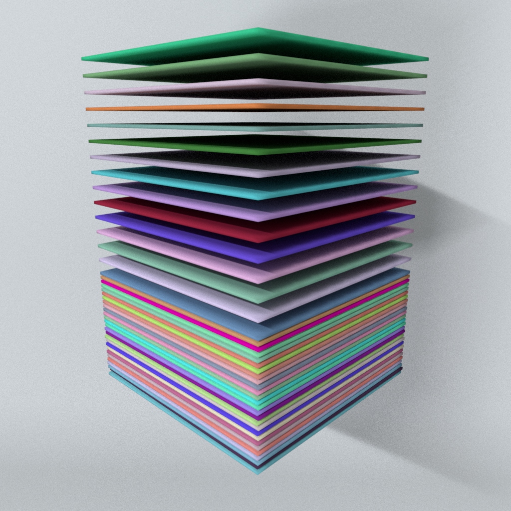
(a) Falling mats

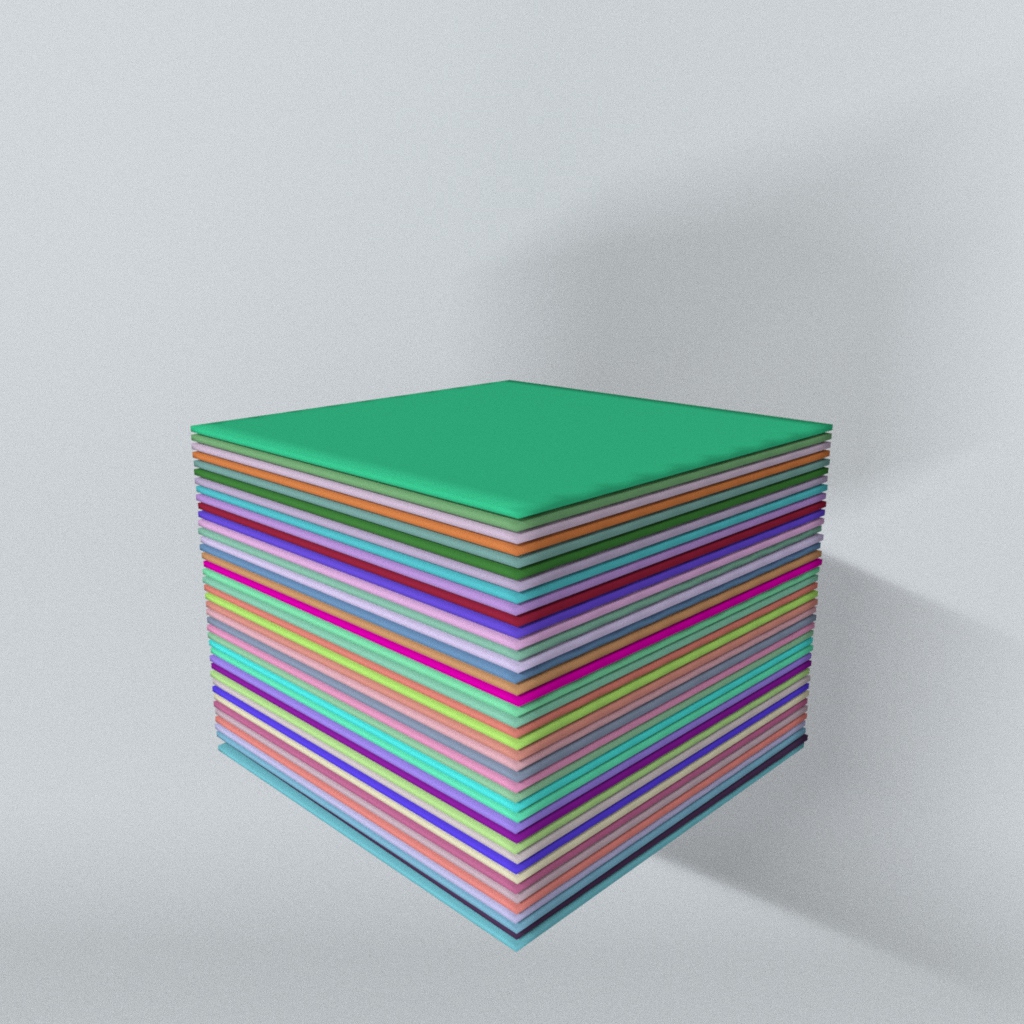
(b) Stacked mats

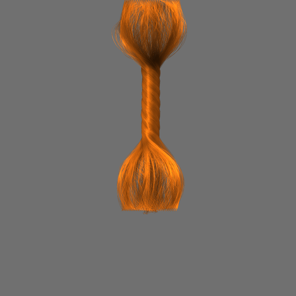
(c) Twisted hair

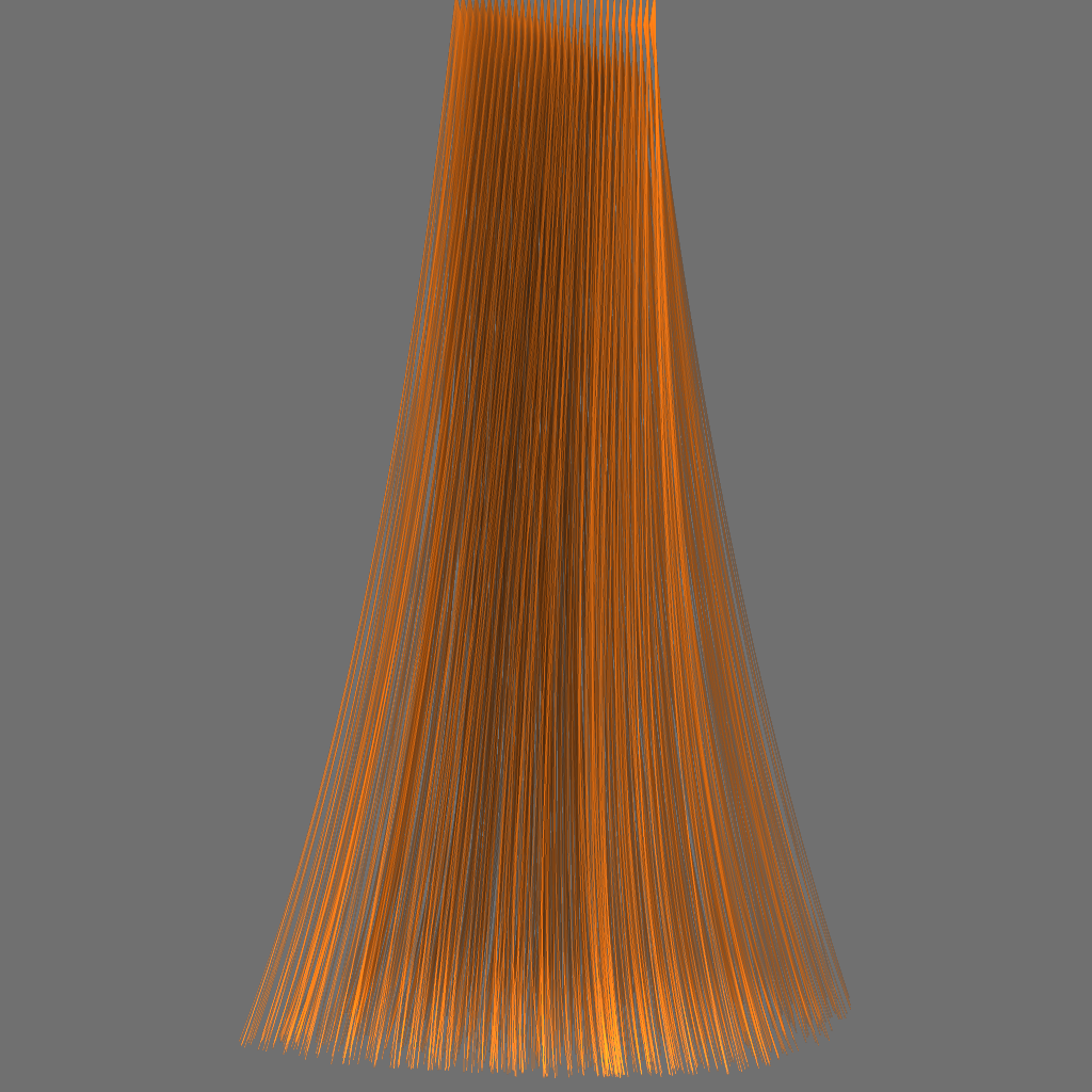
(d) Loose hair

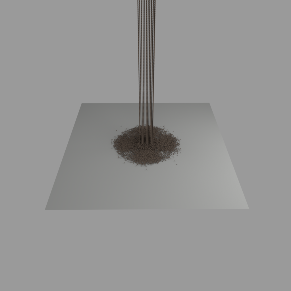
(e) Falling sand

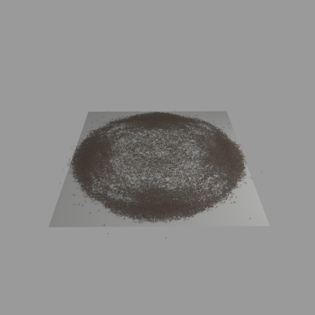
(f) Piled sand

Figure 3. Codimensional deformable bodies. Based on the volume enforcement idea, we develop contact constraints for a wide range of primitive proximity pairs. These contact constraints allow our method to simulate a variety of codimensional examples, including elastic mats in (a) and (b), cloth, hair in (c) and (d), and sand in (e) and (f).

4. The Backward Step

The backward step in our two-way approach is similar to the impact zone optimizations in (Harmon et al., 2008; Narain et al., 2012; Tang et al., 2016, 2018b, 2018a; Li et al., 2020b). Instead of directly performing CCD to find a strictly intersection-free projection, we roughly optimize an intermediate target $\mathbf{y}^{(l)}$ almost intersection-free. Note that it is only used for guiding the vertex advancement in the forward step later, where the exact intersection-freeness is imposed as discussed in Section 5.

In the $l$-th iteration, the goal of the backward step is to project $\mathbf{y}^{(l)}$ back to $\Omega$ formulated as a constrained optimization:

(5) $$\mathbf{y}^{(l+1)}=\mathop{\arg\min}\limits_{\mathbf{y}}\frac{1}{2}\big{\|}\mathbf{y}-{\mathbf{y}}^{[k+1]}\big{\|}^{2}_{\mathbf{M}},\quad\mathrm{s.t.}\;\mathbf{c}(\mathbf{y})\geq\mathbf{0},$$

where $\mathbf{c}(\mathbf{y})\geq\mathbf{0}$ contains the contact constraints and edge length constraints, and $\mathbf{y}$ is initialized with $\mathbf{y}^{(l)}$. Let $\mathbf{x}^{(l)}$ be the current state of the forward step in the $l$-th iteration. We linearize the contact constraints at $\mathbf{x}^{(l)}$: $\mathbf{c}(\mathbf{x}^{(l)})+\mathbf{J}^{(l)}(\mathbf{y}-\mathbf{x}^{(l)})\geq\mathbf{0}$, in which $\mathbf{J}^{(l)}={\partial\mathbf{c}(\mathbf{x}^{(l)})}/{\partial\mathbf{x}}$ is the Jacobian matrix.

Linearization

Note that we perform assembly and linearization of contact constraints at $\mathbf{x}^{(l)}$ rather than $\mathbf{y}^{(l)}$. The reason is that we not only require $\mathbf{y}^{(l+1)}$ to be close to intersection-free, but also expect the path from $\mathbf{x}^{(l)}$ to $\mathbf{y}^{(l+1)}$ to stay inside $\Omega$ as much as possible. Since $\mathbf{x}^{(l)}$ is inside $\Omega$ in the first place, we are actually attempting to drive $\mathbf{y}^{(l+1)}$ to cross the boundary of $\Omega$ and stay on the same side as $\mathbf{x}^{(l)}$ rather than $\mathbf{y}^{(l)}$. Simply projecting the target back to $\Omega$ based on the constraints assembled around $\mathbf{y}^{(l)}$ can cause the stagnation issue as shown in Fig. 4(b), while performing the linearization at $\mathbf{x}^{(l)}$ effectively avoids such an issue and reach the convergence with a more reasonable solution as shown in Fig. 4(c).

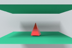
(a) $\mathbf{x}^{[k]}$ (above) and $\mathbf{y}^{[k+1]}$ (below)

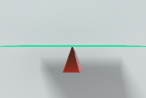
(b) $\mathbf{x}^{[k+1]}$ using the contact constraints assembled around $\mathbf{y}^{(l)}$

(c) $\mathbf{x}^{[k+1]}$ using the contact constraints assembled around $\mathbf{x}^{(l)}$

Figure 4. Linearization choices. The tunneling artifact appears between two intersection-free states $\mathbf{x}^{[k]}$ and $\mathbf{y}^{[k+1]}$ (Fig. (a)). Projecting $\mathbf{y}^{[k+1]}$ back to $\Omega$ based on the constraints assembled around $\mathbf{y}^{(l)}$ stagnates $\mathbf{x}^{[k+1]}$ (Fig. (b)). Instead, if we assemble and linearize contact constraints around $\mathbf{x}^{(l)}$, $\mathbf{y}^{(l)}$ manages to cross the boundary of $\Omega$ and stay on the same side as $\mathbf{x}^{(l)}$, eventually advancing $\mathbf{x}^{(l)}$ to a more reasonable solution (Fig. (c)).

By introducing Lagrangian multipliers, we formulate the following Lagrangian:

(6) $$\mathcal{L}(\mathbf{y},\boldsymbol{\lambda})=\frac{1}{2}\big{\|}\mathbf{y}-\mathbf{y}^{[k+1]}\big{\|}^{2}_{\mathbf{M}}-{\left(\mathbf{c}\big{(}\mathbf{x}^{(l)}\big{)}+\mathbf{J}^{(l)}\big{(}\mathbf{y}-\mathbf{x}^{(l)}\big{)}\right)}^{\mathsf{T}}\boldsymbol{\lambda},$$

whose minimizer satisfies the KKT conditions:

(7) $$\left\{\begin{array}[]{l}\nabla_{\mathbf{y}}\mathcal{L}=\mathbf{M}(\mathbf{y}-{\mathbf{y}}^{[k+1]})-\big{(}\mathbf{J}^{(l)}\big{)}^{\mathsf{T}}\boldsymbol{\lambda}=\mathbf{0},\\ \boldsymbol{\lambda}\geq 0\perp\mathbf{c}\big{(}\mathbf{x}^{(l)}\big{)}+\mathbf{J}^{(l)}\big{(}\mathbf{y}-\mathbf{x}^{(l)}\big{)}\geq\mathbf{0}.\end{array}\right.$$

Multiplying the first condition in Eq. 7 with $\mathbf{J}^{(l)}$, we obtain:

(8) $$\mathbf{J}^{(l)}\mathbf{y}=\mathbf{J}^{(l)}\mathbf{M}^{-1}\big{(}\mathbf{J}^{(l)}\big{)}^{\mathsf{T}}\boldsymbol{\lambda}+\mathbf{J}^{(l)}{\mathbf{y}}^{[k+1]}.$$

Together with the second condition, we get a linear complementarity problem (LCP) with only one unknown $\boldsymbol{\lambda}$:

(9) $$\boldsymbol{\lambda}\geq\mathbf{0}\perp\mathbf{c}\big{(}\mathbf{x}^{(l)}\big{)}+\mathbf{J}^{(l)}\mathbf{M}^{-1}\big{(}\mathbf{J}^{(l)}\big{)}^{\mathsf{T}}\boldsymbol{\lambda}+\mathbf{J}^{(l)}\big{(}{\mathbf{y}}^{[k+1]}-{\mathbf{x}}^{(l)}\big{)}\geq\mathbf{0}.$$

Once we solve $\boldsymbol{\lambda}$, we apply the first condition of Eq. (7) to calculate $\mathbf{y}^{(l+1)}$ for the next iteration. Note that $\mathbf{y}^{(l)}$ is the initialization to the problem in Eq. (5) and it is calculated from the last $\boldsymbol{\lambda}$ in the ($l$-1)-th step, so the cumulative effect of the previous $l$-1 iterations to $\mathbf{y}$ is retained.

4.1. Contact Constraints

An interesting question is how to define the contact constraints $\mathbf{c}(\mathbf{x})\geq\mathbf{0}$ for a variety of primitive proximity pairs. In our method, we construct our contact constraints in a volume enforcement fashion.

Figure 5. Vertex-triangle pair. Our constraint enforces the volume of $\mathbf{x}_{a}\mathbf{x}_{i}\mathbf{x}_{j}\mathbf{x}_{k}$ to be the same as its reference $\mathbf{r}_{a}\mathbf{r}_{i}\mathbf{r}_{j}\mathbf{r}_{k}$ (Fig. (a)), in which the vertex and the triangle are separated by a threshold distance $\delta$ (Fig. (b)). Tessellated with small tetrahedra in crevices, the simulated cloth robustly prevents self-intersections (Fig. (c)).

To begin with, we consider a vertex-triangle proximity pair in Fig. 5(a), whose distance is below a certain activation threshold $\delta$. In our experiment, $\delta$=1mm. Let $\{\mathbf{r}_{a},\mathbf{r}_{i},\mathbf{r}_{j},\mathbf{r}_{k}\}$ be its projection, calculated by moving the vertex and the triangle in opposite normal directions until the distance becomes $\delta$:

(10) $$\left\{\begin{array}[]{l}\mathbf{r}_{a}\quad=\mathbf{x}_{a}\quad+\frac{1}{2}\left(\delta-\left\|\mathbf{x}_{a}-b_{i}\mathbf{x}_{i}-b_{j}\mathbf{x}_{j}-b_{k}\mathbf{x}_{k}\right\|\right)\mathbf{n},\\ \mathbf{r}_{i,j,k}=\mathbf{x}_{i,j,k}-\frac{1}{2}\left(\delta-\left\|\mathbf{x}_{a}-b_{i}\mathbf{x}_{i}-b_{j}\mathbf{x}_{j}-b_{k}\mathbf{x}_{k}\right\|\right)\mathbf{n},\end{array}\right.$$

where $b_{i}$, $b_{j}$ and $b_{k}$ are the barycentric weights of vertex $a$ on the triangle, and $\mathbf{n}$ is the constant triangle normal. Under the assumption that the triangle area is constant, we define the contact constraint by requiring the volume of $\mathbf{x}_{a}\mathbf{x}_{i}\mathbf{x}_{j}\mathbf{x}_{k}$ to be greater than or equal to the volume of $\mathbf{r}_{a}\mathbf{r}_{i}\mathbf{r}_{j}\mathbf{r}_{k}$:

(11) $$\quad c(\mathbf{x}_{a},\mathbf{x}_{i},\mathbf{x}_{j},\mathbf{x}_{k})=\mathsf{det}({\partial{\mathbf{x}}}/{\partial{\mathbf{r}}})-1\geq 0,$$

in which $\mathbf{r}_{a}$, $\mathbf{r}_{i}$, $\mathbf{r}_{j}$ and $\mathbf{r}_{k}$ are treated as constants, and $\partial{\mathbf{x}}/{\partial{\mathbf{r}}}$ is the artificial deformation gradient tensor, assuming that the computed $\mathbf{r}$ is the reference shape. Note that the contact constraint actually outlines the boundary of the feasible region at $\mathbf{x}^{(l)}$, so the sign of volume at $\mathbf{x}^{(l)}$ is positive. If $\mathbf{y}^{(l)}$ is on the other side of the boundary, the sign of volume at $\mathbf{y}^{(l)}$ would be negative and the inequality constraint would “pull” $\mathbf{y}^{(l)}$ to the same side as $\mathbf{x}^{(l)}$.

Based on the same idea, we model the contact constraints for other simplex pairs, including edge-edge pairs, and vertex-vertex pairs. In the simplest case, the contact constraint for a vertex-vertex pair is:

(12) $$c(\mathbf{x}_{a},\mathbf{x}_{i})=\left\|\mathbf{x}_{i}-\mathbf{x}_{a}\right\|/\delta-1\geq 0.$$

These constraints enable our method to handle contacts for a variety of codimensional deformable body examples, such as cloth, hair (in Fig. 3(c) and 3(d)) and sand (in Fig. 3(e) and 3(f)).

We find such volume-based constraints do not suffer from locking artifacts, which usually come from the edge-edge pairs. The possible reason is that if we renew the reference volume in every intermediate step as our method does, it does not cause the resistance of shearing or twisting, whereas if the reference shapes are constant, these artifacts would be observed as discussed in  (Müller et al., 2015). A potential problem with volumetric constraints is that they may increase the triangle area or edge length, which may influence the simulation quality or performance negatively. However, this issue is barely problematic in our experiments: we test the popular gap constraints (Andrews et al., 2022) as a replacement, and using both kinds of constraints has comparable performances as Fig. 6 shows, and our examples show that volumetric constraints can work well without obvious artifacts.

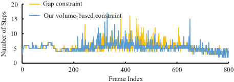
(a) The number of steps fluctuating over frames

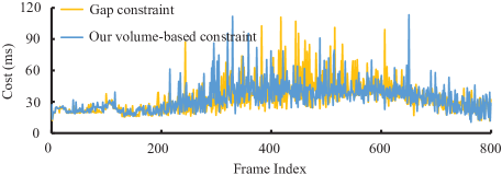
(b) The collision cost fluctuating over frames

Figure 6. Comparison with the gap constraints. We count the performances of our method implemented with the gap constraints and the volume-based constraints (as ours). Our volume-based constraints have comparable performance compared with the gap constraints and do not have a negative influence on performance. By default, we use the bow knot example for evaluations in this paper.

Sifakis et al. (2008) explored a similar idea, but they chose to preserve the volume, rather than enforce the volume to a desired value. In comparison, our constraints can keep pairs well separated, so that fewer collisions can occur in later updates.

4.2. Edge length Constraints

When the target $\mathbf{y}^{[k+1]}$ is close to $\mathbf{x}^{[k]}$, minimizing the mass-weighted Euclidean distance keeps a minimal change of kinetic energy after collision handling and the change of potential should not be significant either. However, as $\mathbf{y}^{[k+1]}$ starts to get far away from $\mathbf{x}^{[k]}$, simply using this kinetic energy norm to measure the projection distance could be inappropriate. It can cause spuriously large, local deformations (see Figs. 17 and 18) and even oscillations over time, as a result of a sharp change of potential before and after collision handling. We can incorporate additional deformation resistance terms into the objective function, but it breaks a simple LCP formulation and thus is more numerically involved. Given the fact that potentials are basically penalizing non-rigid deformations, we therefore attempt to preserve the shape of each element by preserving its edge lengths, so that each element mostly undergoes a rigid transformation and the change of potential stays at a low level after collision handling.

For keeping it as a simple LCP formulation where many fast iterative techniques can be used, we follow the strategy in (Macklin and Muller, 2021) to suppress spurious distortions by incorporating constraints without complicating the objective function, and linearize it at $\mathbf{y}^{[k+1]}$:

(13) $$c(\mathbf{x}_{i},\mathbf{x}_{j})=\sigma-{\big{\|}\mathbf{x}_{i}-\mathbf{x}_{j}\big{\|}\mathord{\left/{\vphantom{\big{\|}\mathbf{x}_{i}-\mathbf{x}_{j}\big{\|}\big{\|}\mathbf{y}_{i}^{[k+1]}-\mathbf{y}_{j}^{[k+1]}\big{\|}}}\right.\kern-1.2pt}\big{\|}\mathbf{y}_{i}^{[k+1]}-\mathbf{y}_{j}^{[k+1]}\big{\|}}\geq 0,$$

in which $i$ and $j$ are the two vertex indices of one edge and $\sigma$ is the maximum violation ratio. Here we relax the strict bilateral constraint to the soft unilateral one and permit a certain level of violation for performance consideration.

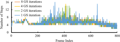
(a) The number of steps fluctuating over frames

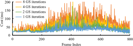
(b) The collision cost fluctuating over frames

Figure 7. Performance w.r.t. Gauss-Seidel iterations. We count the performances of our method with different numbers of Gauss-Seidel iterations per backward step. By applying more Gauss-Seidel iterations, we can solve the LCP problem more accurately in every backward step, but it does not necessarily reduce the number of steps (Fig. (a)). Thus, we recommend using only one Gauss-Seidel iteration per step for the efficiency purpose (Fig. (b)).

4.3. An Inexact GPU-Based Optimizer

A popular way of solving the LCP problem in Eq. (9) is to apply a projected iterative method (Erleben, 2013), which enforces $\boldsymbol{\lambda}\geq\mathbf{0}$ after every iteration solving the linear system. In our simulator, we adopt standard multi-color Gauss-Seidel as our solver. We use the randomized graph coloring method in  (Fratarcangeli et al., 2016) while we assign color (graph node) to constraints, not vertices. This is different from the strategy in (Fratarcangeli et al., 2016). Please refer to (Fratarcangeli et al., 2016) for more details.

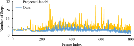
(a) The number of steps fluctuating over frames

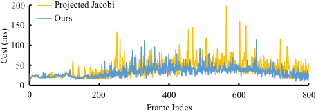
(b) The collision cost fluctuating over frames

Figure 8. Comparison with projected Jacobi method. We count the performances of our method implemented with the projected Jacobi method and the projected Gauss-Seidel method (as ours). Compared with ours, using projected Jacobi needs more steps (Fig. (a)) to conditionally converge under metric $\mathbf{r}$ and thus more computational costs (Fig. (b)).

4.3.1. Inexactness

One interesting question is how many iterations should we spend on solving the LCP problem? The more iterations we use, the more exactly we get the problem solved. But given the fact that we face a new LCP problem in the next backward step, it will be a waste if we spend too much computational cost on a single problem. Ultimately, our choice should be based on the total collision cost, fundamentally determined by two factors: the total number of steps for reaching convergence and the costs associated with backward and forward steps. According to Fig. 7, increasing the number of Gauss-Seidel iterations negatively affects the overall performance. Therefore, we choose to use a single iteration per backward step by default.

4.3.2. A projected Jacobi implementation

The analysis in Subsection 4.3.1 motivates us to consider an even more inexact implementation, i.e., replacing one projected Gauss-Seidel iteration by one projected Jacobi iteration. After testing this implementation, we conclude that it is not a suitable choice for two reasons. First, projected Jacobi needs an under-relaxation factor to ensure its convergence, which further lowers the convergence rate. Second, the nonsmooth nature of our method makes Chebyshev acceleration (Wang, 2015) ineffective across steps. Overall, the method with projected Jacobi needs more steps and more costs for collisions as Fig. 8 shows.

4.4. Comparison to An Augmented Lagrangian Optimizer

We can adopt other constrained optimization techniques to perform the task in our backward step as well. Specifically, we would like to evaluate the performance of an augmented Lagrangian optimizer with the gradient descent method, advocated by Tang et al. (2018b). The strength of their optimizer is its simplicity: it does not need to solve any system for primal or dual variables, and the only major computational components are gradient and constraint evaluations. But since their optimizer converges considerably slower, the method with their optimizer must run multiple iterations per backward step to reduce the total number of steps. In our experiment, we implement their optimizer with two options: one running 20 iterations per step and one running 100 iterations per step. We find when we use fewer iterations of their optimizer, its ability to change $\mathbf{r}$ degenerates very quickly. To avoid iterations with no revenue for their optimizer, if we find after one step, the change of $\big{\|}\mathbf{r}\big{\|}_{\infty}$ is tiny ($\big{\|}\mathbf{r}^{(l)}\big{\|}_{\infty}-\big{\|}\mathbf{r}^{(l+1)}\big{\|}_{\infty}$¡FLT_EPSILON), the collision handling module terminates immediately. Fig. 9 shows that when using 20 iterations per step, the two-way method with their optimizer needs a large number of steps and often early terminates, especially when the knot is tight. When increasing to 100 iterations per step, the early termination could be alleviated, but the two-way method with their optimizer still needs a large number of steps compared with ours which is always terminated under metric $\mathbf{r}$ in a small time consumption. Overall our optimizer is a better choice.

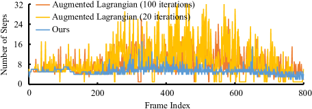
(a) The number of steps fluctuating over frames

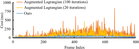
(b) The collision cost fluctuating over frames

Figure 9. Comparison with augmented Lagrangian method. We compare the performance of our own optimizer and the augmented Lagrangian optimizer in (Tang et al., 2018b). Since their optimizer converges significantly slower than ours, it has to run multiple iterations per backward step to reduce the total number of steps. However, the improved convergence does not pay off the extra cost, which makes their method less efficient.

5. The Forward Step

In each forward step, we move the vertices from the current state $\mathbf{x}^{(l)}$ toward ${\mathbf{y}}^{(l+1)}$ asynchronously:

(14) $${\mathbf{x}}_{i}^{(l+1)}={\mathbf{x}}_{i}^{(l)}+\alpha_{i}^{(l+1)}\big{(}{\mathbf{y}}_{i}^{(l+1)}-{\mathbf{x}}_{i}^{(l)}\big{)}.$$

The key question is how to find the safe step size $\alpha_{i}^{(l+1)}$ for every vertex $i$, so that $\mathcal{X}(\mathbf{x}^{(l)},\mathbf{x}^{(l+1)})\subset\Omega$. One way of obtaining a safe step size is to use continuous collision detection (CCD). CCD tests calculate exact moments when proximity pairs intersect, using which we then determine how far $\mathbf{x}_{i}$ can travel. However, previous works show that CCD tests could be prone to errors  (Ainsley et al., 2012; Wang, 2014; Tang et al., 2014) and require considerable efforts to get accelerated on GPUs (Tang et al., 2011a, 2018b, 2016).

In our method, we propose to use an inexpensive yet reliable scheme for calculating the safe step size. Our key idea is based on the simple fact that a proximity pair cannot intersect, if none of its vertices moves more than half of its distance. To use this idea, the method needs a set of proximity pairs $\mathcal{P}$, in which each pair contains two non-adjacent simplices with its distance below a global threshold $D^{(l)}$. Given $\mathcal{P}$, the method calculates $D_{i}$, the shortest distance of the proximity pairs involving vertex $i$:

(15) $$D_{i}=\min\limits_{\{a,\,b\}\in\mathcal{P}}\mathtt{dist}\big{(}\mathbf{x}_{a}^{(l)},\mathbf{x}_{b}^{(l)}\big{)}\leq D^{(l)},\,\forall a,b:a\neq b\;\mathrm{and}\;i\in a\cup b.$$

in which $a$ and $b$ are the two simplices and $\mathtt{dist}\big{(}\mathbf{x}_{a}^{(l)},\mathbf{x}_{b}^{(l)}\big{)}$ is their distance. We treat $D_{i}/2$ as an upper bound on the displacement of vertex $i$ to ensure the intersection-free condition:

(16) $$\forall i:\;{\big{\|}\mathbf{x}_{i}^{(l)}-\mathbf{x}_{i}^{(l+1)}\big{\|}}<D_{i}/2\Rightarrow(1-t)\mathbf{x}^{(l)}+t\mathbf{x}^{(l+1)}\in\Omega,$$

for any $t\in[0,1]$. Therefore we formulate our forward step by updating the position of vertex $i$ as:

(17) $$\left\{\begin{array}[]{l}\alpha_{i}^{(l+1)}=\min\left({{{0.5\gamma{D_{i}}}\mathord{\left/{\vphantom{{0.5\gamma{D_{i}}}{\big{\|}{\mathbf{y}_{i}^{(l+1)}-\mathbf{x}_{i}^{(l)}}\big{\|}}}}\right.\kern-1.2pt}{\left\|{\mathbf{y}_{i}^{(l+1)}-\mathbf{x}_{i}^{(l)}}\right\|}},1}\right),\\ \mathbf{x}_{i}^{(l+1)}=\mathbf{x}_{i}^{(l)}+\alpha_{i}^{(l+1)}\big{(}{\mathbf{y}_{i}^{(l+1)}-\mathbf{x}_{i}^{(l)}}\big{)},\\ r_{i}^{(l+1)}=r_{i}^{(l)}\big{(}1-\alpha_{i}^{(l+1)}\big{)},\end{array}\right.$$

in which $\gamma$ is a damping factor preventing proximity pairs from getting too close in a single forward step. Using the step size calculated for every vertex, we ensure that $\mathbf{x}^{(l+1)}$ is an acceptable intermediate state, regardless of the search direction.

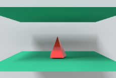
(a) $\mathbf{x}^{[k]}$ (above) and $\mathbf{y}^{[k+1]}$ (below)

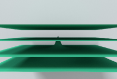
(b) stack view of $\mathbf{x}^{[k+1]}$ with various $\epsilon$

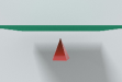
(c) $\mathbf{x}^{[k+1]}$ with $\epsilon=0.75$

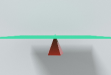
(d) $\mathbf{x}^{[k+1]}$ with $\epsilon=0.50$

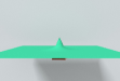
(e) $\mathbf{x}^{[k+1]}$ with $\epsilon=0.25$

(f) $\mathbf{x}^{[k+1]}$ with $\epsilon=0.0001$

Figure 10. Termination condition and threshold $\boldsymbol{\epsilon}$. With the same $\mathbf{x}^{[k]}$ and $\mathbf{y}^{[k+1]}$, the accumulated moving distance from $\mathbf{x}^{[k]}$ to $\mathbf{x}^{[k+1]}$ is getting close to the distance from $\mathbf{x}^{[k]}$ to $\mathbf{y}^{[k+1]}$ as $\epsilon$ approaching zero, reducing the risk of early termination.

A special feature we would like to mention in Eq. (17) is the termination metric $r_{i}$. The non-smooth nature of our optimization method makes it difficult to define the termination condition by the step size $\alpha_{i}^{(l+1)}$ directly, without potential early termination risks. To address this issue, we come up with a termination metric $r_{i}$ in an accumulated fashion. Intuitively, it keeps track of the remaining step size needed for vertex $i$ to reach its target and we terminate the method once $\|\mathbf{r}^{(l+1)}\|_{\infty}$ drops below a certain threshold $\epsilon$. As the threshold $\epsilon$ tends to zero, the accumulated moving distance from $\mathbf{x}^{[k]}$ to $\mathbf{x}^{[k+1]}$ tends to be close enough to the distance from $\mathbf{x}^{[k]}$ to $\mathbf{y}^{[k+1]}$, so the early termination risks of the optimization could be eliminated as shown in Fig. 10(f).

Compared with CCD tests, distance evaluations used by our scheme are computationally inexpensive, reliable against floating-point errors and easy to parallelize on GPUs.

5.1. Comparison to CCD-Based Schemes

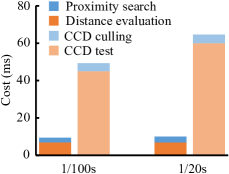
Figure 11. Comparison with CCD. Overall, the total cost of CCD-free step size schemes by the collision handling process is five to seven times faster than CCD-based schemes in a time step.

To compare our CCD-free step size scheme with CCD-based schemes, we implement a CCD-based scheme by the tests provided by I-Cloth (Tang et al., 2018b), which is one of the fastest CCD implementations on a GPU. We also adjust both schemes to use the same proximity search tool provided by I-Cloth, so that we can eliminate the difference in the implementations of proximity search. On the same NVIDIA GeForce GTX 2080 Ti GPU, we evaluate both schemes in a number of examples with two large time steps: $\Delta t$=1/100s and $\Delta t$=1/20s.

In the examples with $\Delta t$=1/100s, the experiment shows our proximity search cost is about 60 percent of the broad-phase CCD culling cost, while the distance evaluation cost is about 15 percent of the narrow-phase CCD test cost. Together our CCD-free scheme is five times faster than the CCD-based scheme.

In the examples with $\Delta t$=1/20s, the narrow-phase CCD test cost increases significantly while the distance evaluation cost increases marginally. As a result, our CCD-free scheme is about seven times faster than the CCD-based scheme.

We note that the computational costs of the two step size schemes alone do not provide the full picture of their difference. In general, our CCD-free scheme provides smaller step sizes and causes 10 to 20 percent more steps needed for convergence. This further increases the cost of the backward step by 10 to 20 percent. But overall, it is still beneficial to use the CCD-free scheme, given the large computational cost needed for CCD tests.

The Special CCD-Based Scheme in (Wu et al., 2020)

The step size scheme adopted by the hard phase in (Wu et al., 2020) is also based on CCD tests. Compared with other CCD-based schemes, their approach restricts all of the edge lengths to be less than a constant upper bound, and accordingly derives a series of sufficient conditions to prevent intersections, which can be achieved by handling vertex-vertex contacts only. As a result, their CCD tests are less expensive, making their method suitable for fast simulation of virtual garments that are almost inextensible.

However, such a benefit comes at the cost of limited applicability. If we apply their scheme to simulate general shell deformations where this length restriction can not be adopted, e.g., the sustaining inflation or contraction of membrane in the normal flow example (Fig. 20), then CCD tests have to consider all necessary vertex-triangle and edge-edge contacts again. In such cases, their method would be less efficient.

6. Implementation Details

In this section, we discuss the implementation details of our two-way method in a GPU-based deformable body simulator.

6.1. Dynamics Solvers

Since our method works as a standalone module for collision handling, it is naturally compatible with most of the dynamics solvers. In our simulator, we follow the pipeline in Eq. (2) to solve the nonlinear optimization problem stemming from deformable body dynamics. In detail, $Q_{k}$ is a quadratic proxy of energies written as below:

(18) $$Q_{k}={{E}\big{(}\mathbf{x}^{[k]},\mathbf{x}^{t},\mathbf{v}^{t}\big{)}}+{\mathbf{b}^{[k]}}^{\intercal}(\mathbf{y}-\mathbf{x}^{[k]})+\frac{1}{2}(\mathbf{y}-\mathbf{x}^{[k]})^{\intercal}\mathbf{G}^{[k]}(\mathbf{y}-\mathbf{x}^{[k]}),\quad\;$$

in which $\mathbf{b}^{[k]}$ is the gradient and $\mathbf{G}^{[k]}$ is the modified Hessian of $\left.E(\mathbf{x},\mathbf{x}^{t},\mathbf{v}^{t})\right|_{\mathbf{x}=\mathbf{x}^{[k]}}$ after positive semi-definite projection. We apply the conjugate gradient method with a block Jacobi preconditioner to solve the linear system emerged from the quadratic model in every Newton iteration. We treat the Newton iteration as an update and run our two-way method for collision handling right afterwards. Currently, our simulator uses CUDA 11.2 and the CUB library for reduction and sorting operations.

In our implementation, we fix the number of Newton iterations as a constant. Ideally, this number is related to the time step: the solver should run more Newton iterations as the time step increases for more accurate results. But even if we choose to run a single Newton iteration for a large time step, i.e., $\Delta t$=1/10s, our method still can guarantee intersection-free with much less artifacts compared with existing collision handling algorithms as Fig. 18 shows.

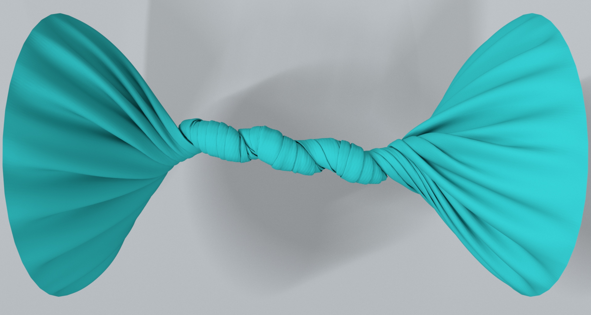
(a) The initial state

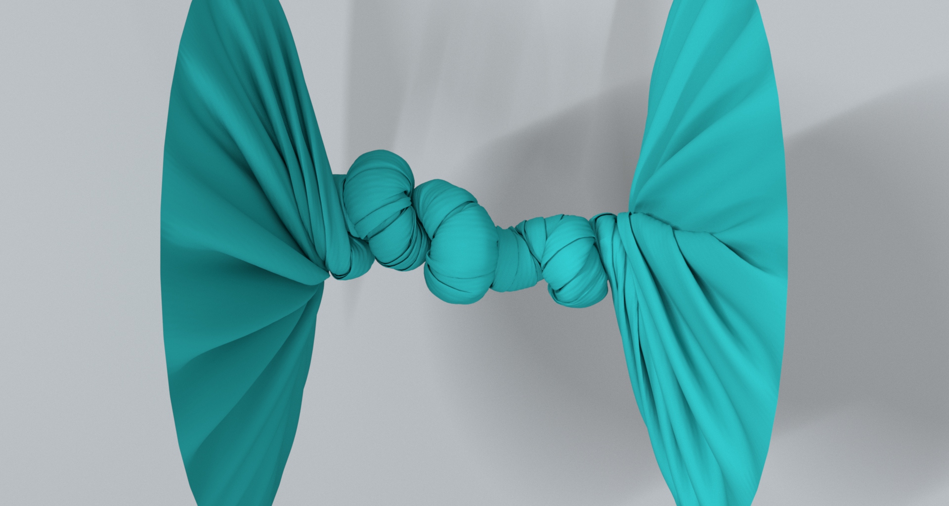
(b) The twisted state

Figure 12. Twisting tube. When a compliant cloth tube is severely squeezed, it experiences intense and frequent collisions in the middle part as shown in (b). Our method robustly handles these collisions in this example taking $\Delta t$=1/100s as the time step.

6.2. Elastic and Repulsive Models

To simulate codimensional deformable body examples shown in Fig. 3, we provide a number of elastic models in our dynamics solver, including the St. Venant-Kirchhoff model for tetrahedral meshes, the co-rotational linear model and the quadratic bending model (Bergou et al., 2006) for triangular meshes, and the mass-spring model for hair strands. The eigensystems of the Hessian matrix for these energy models have been analyzed (Choi and Ko, 2002; Etzmuß et al., 2003; Teran et al., 2005; Smith et al., 2019) and at most only $3\times 3$ singular value decomposition (SVD) is needed for positive semi-definite projection, which can be solved efficiently on GPU (Gao* et al., 2018) or the Hessian matrix is natively guaranteed to be positive semi-definite (Bergou et al., 2006). Some other energy models can also be incorporated into this framework, such as the discrete shell model (Grinspun et al., 2003) where the positive semi-definite projection involving larger matrix eigendecomposition should be done on the CPU like (Li et al., 2021; Chen et al., 2022). Similar to many other simulators (Narain et al., 2012; Tang et al., 2016, 2018b; Li et al., 2020b), our simulator incorporates a quadratic-energy-based repulsive model into deformable body dynamics, to reduce the collision complexity in simulation.

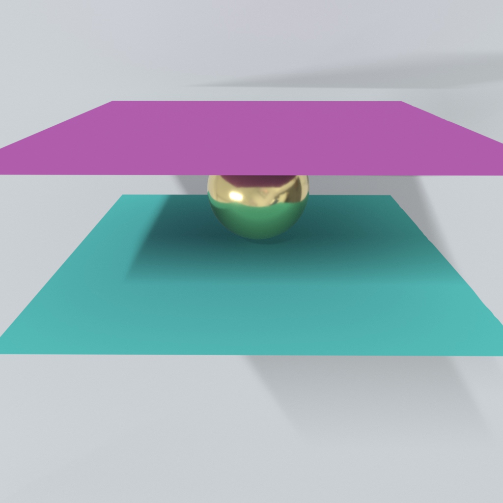
(a) The initial state

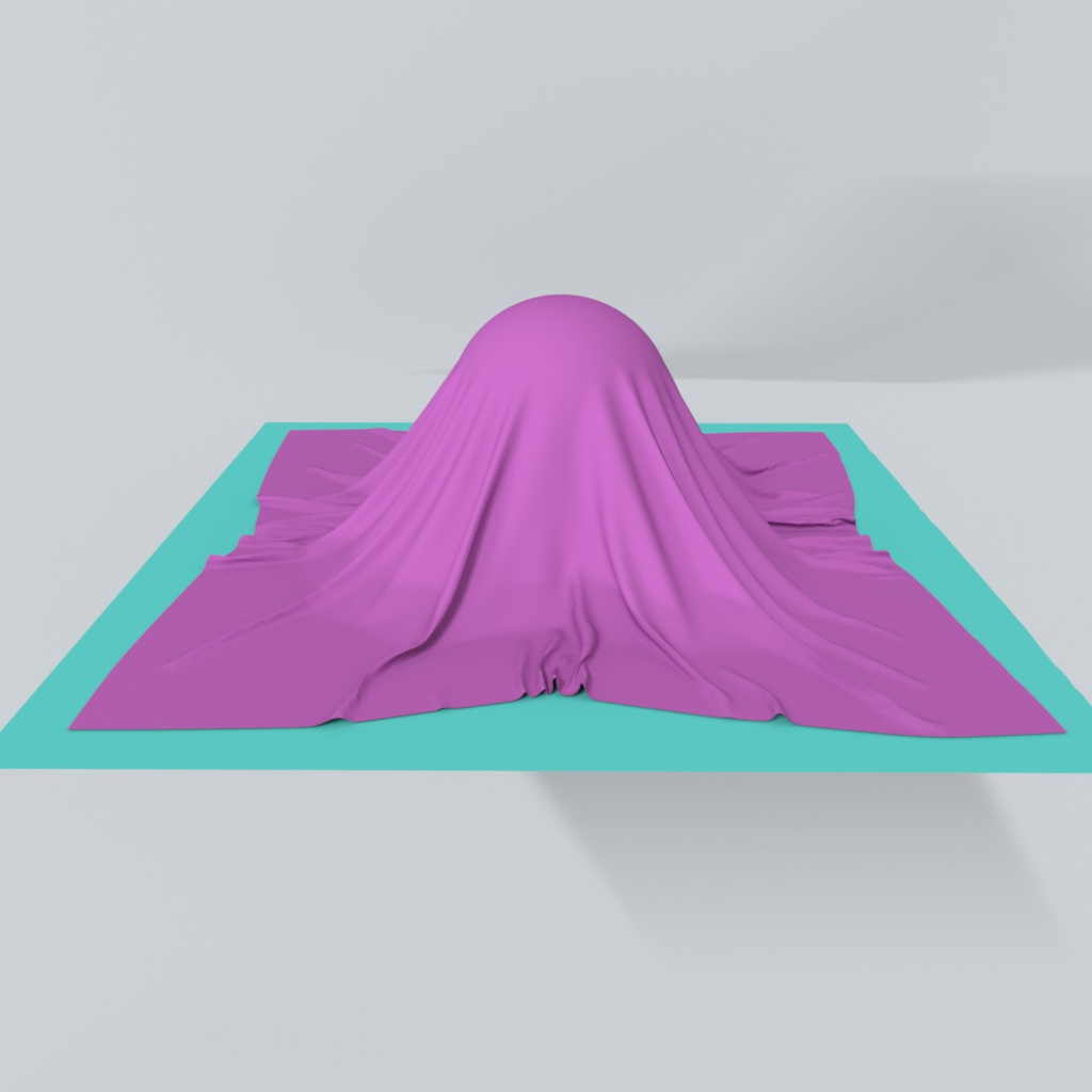
(b) The falling state

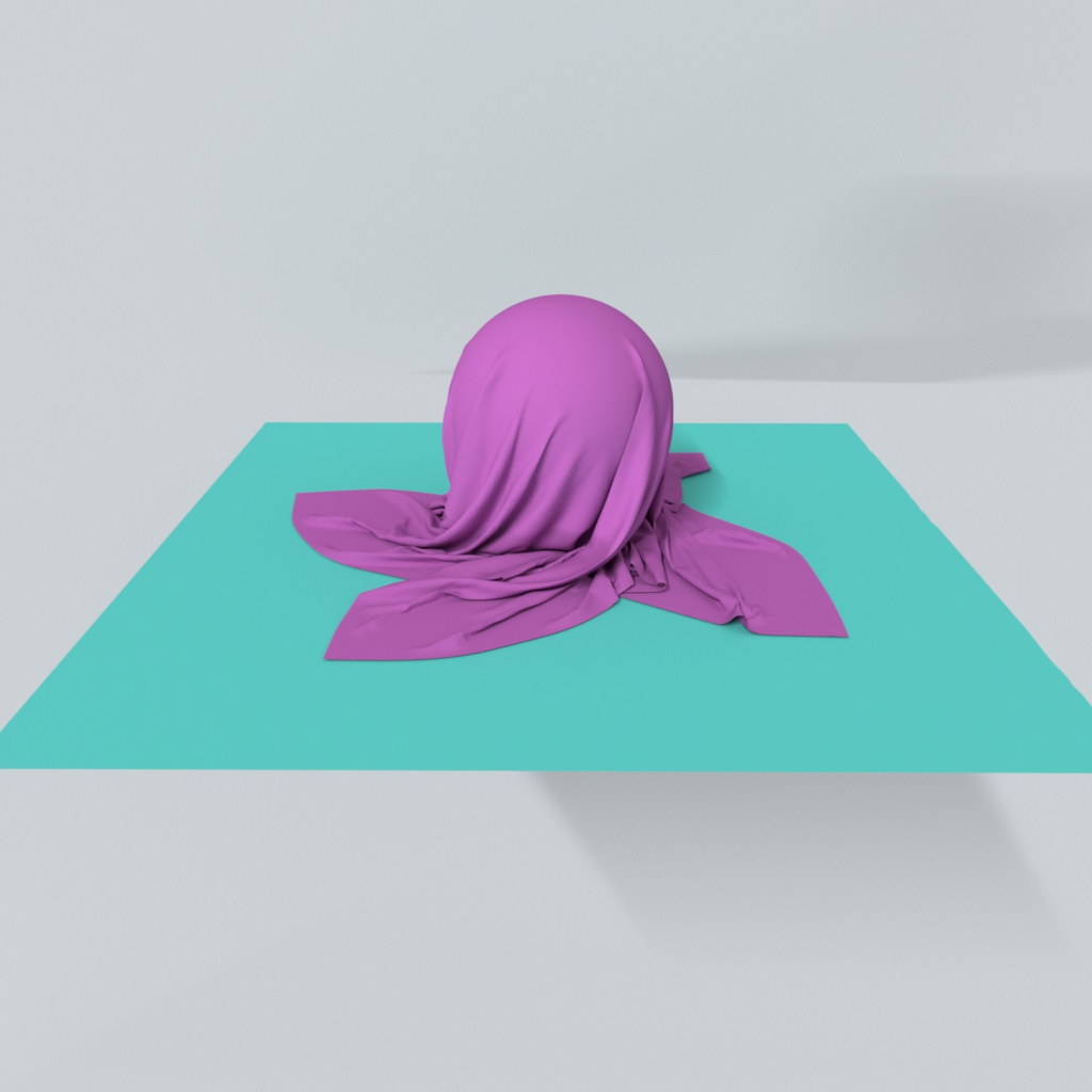
(c) The sliding state

Figure 13. Rotating sphere. When a square cloth patch falls onto a rotating sphere, it forms multiple folds and wrinkles due to its frictional contacts with the sphere and the ground floor.

6.3. Frictional Contacts

We adopt the velocity filtering approach proposed in (Bridson et al., 2002) to handle frictional contacts. First we run the dynamics solver to compute the target state $\mathbf{y}^{[k+1]}$ with no friction. We then calculate penetration depths to estimate collision impulses and use them to determine associated frictional impulses by Coulomb’s law as well. Finally, we update $\mathbf{y}^{[k+1]}$ by both impulses and treat it as the new target state for collision handling. We note that the velocity filtering strategy is more suitable in deformable-rigid body contacts, than in self body contacts, since penetration depth estimations are inaccurate and irrelevant to the actual collision handling process, especially if the time step is large. Fig. 13 demonstrates our current frictional effects achieved by the velocity filtering.

Table 1. Statistics and performances. This table lists the time step size, the maximum and mean numbers of steps and time cost spent by our two-way method in one time step on various examples.

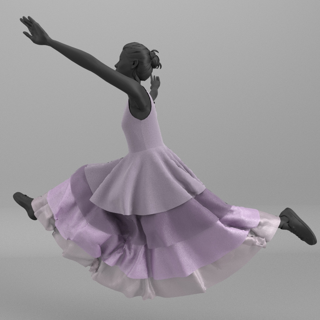
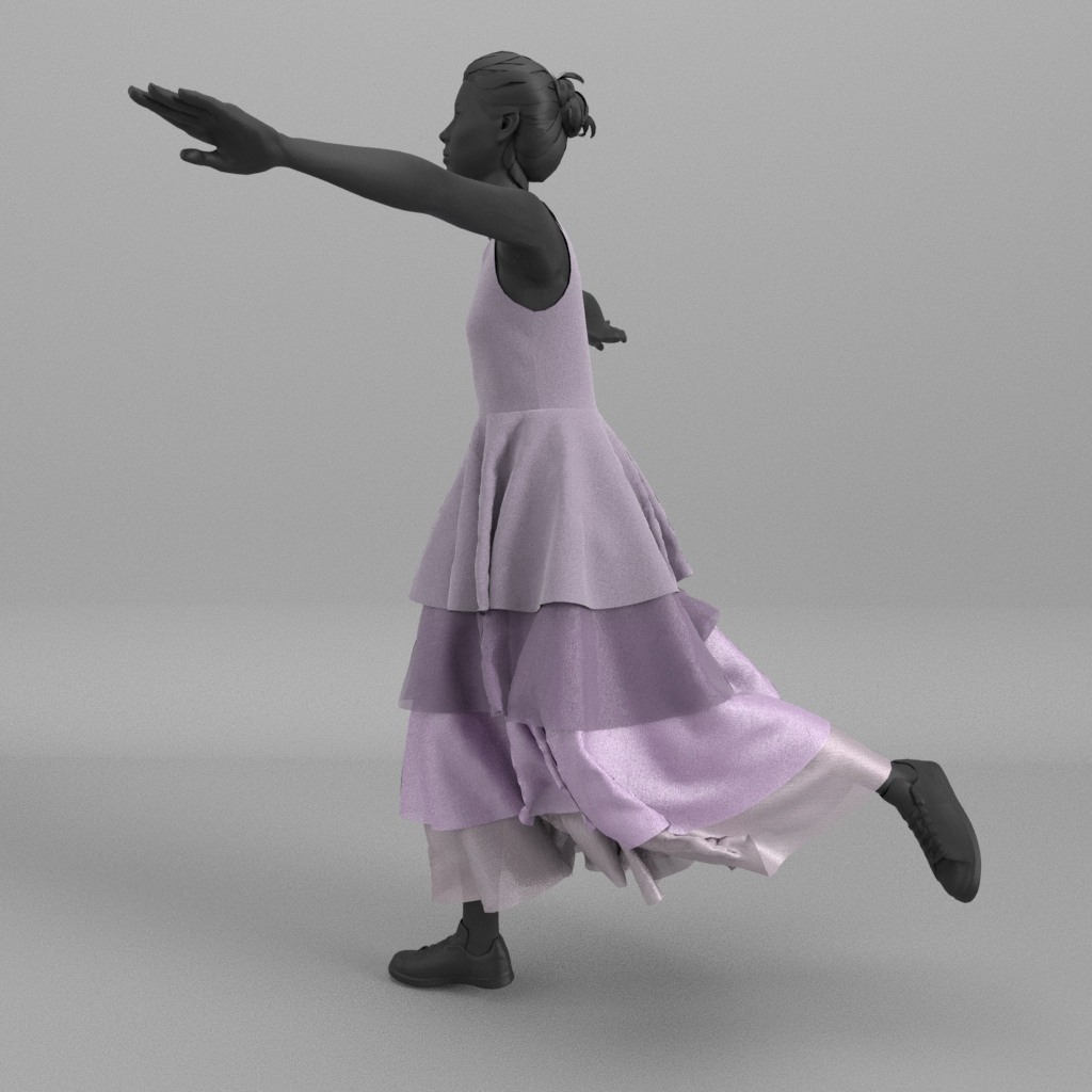
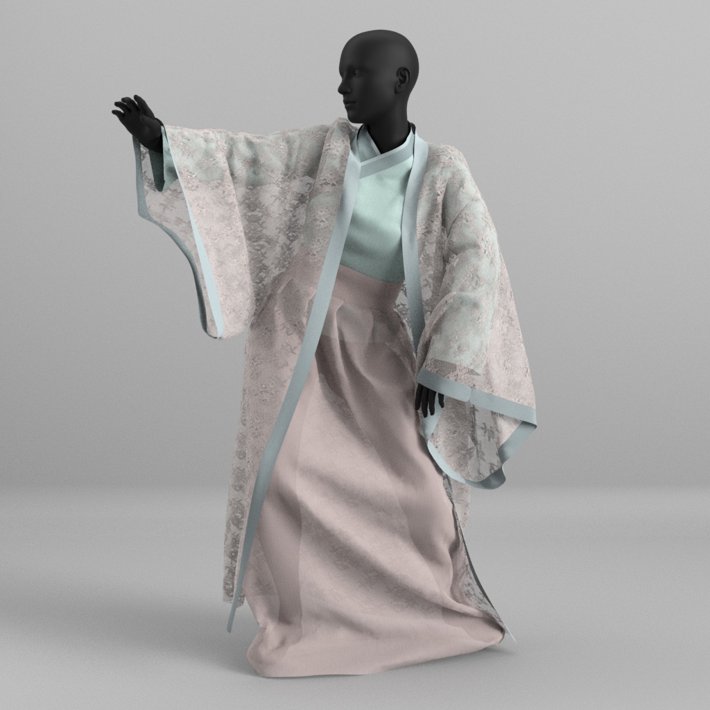
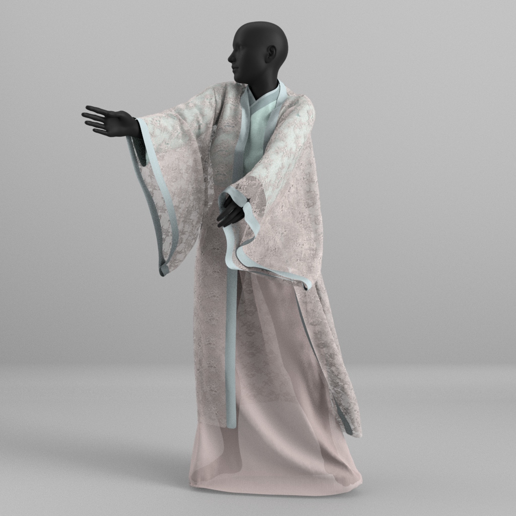
A multi-layered dress		A multi-layered gown

Figure 21. Multi-layered clothing. Our method is capable of handling complex collisions reliably among multiple layers of clothing, produced by these dancing characters.

Name	Time	Avg. (Max.)	Avg. (Max.)
(#verts., #edg./#tri./#tet., ref.)	step (s)	# of steps	cost (s)
Needle (10k, 20k, Fig. 10(f))	1/20	46 (1304)	0.036 (1.942)
Blade (59k, 116k, Fig. 19)	1/20	55 (779)	0.267 (4.463)
Funnel (49K, 98K, Fig. 15a)	1/20	27 (675)	0.087 (2.161)
Funnel (49K, 98K, Fig. 15b)	1/40	23 (437)	0.055 (1.198)
Funnel (49K, 98K, Fig. 15c)	1/80	12 (165)	0.040 (0.776)
Funnel (49K, 98K, Fig. 15d)	1/160	10 (95)	0.029 (0.296)
Sphere (50k, 100k, Fig. 13)	1/100	19 (219)	0.044 (0.475)
Dress (30K, 60K, Fig. 21a)	1/100	39 (142)	0.133 (0.511)
Gown (27K, 51K, Fig. 21c)	1/100	32 (150)	0.092 (0.443)
Bow knot (71K, 142K, Fig. 1a)	1/100	5.4 (17)	0.034 (0.113)
Reef knot (37K, 71K, Fig. 1e)	1/100	7 (23)	0.024 (0.097)
Tube (25k, 51K, Fig. 12)	1/100	19 (54)	0.308 (1.500)
Mat (33k, 88K, Fig. 3a)	1/100	9 (128)	0.020 (0.303)
Hair (63K, 62k, Fig. 3c)	1/100	16 (503)	0.252 (15.821)
Sand (30K, - , Fig. 3e)	1/100	51 (160)	0.223 (1.550)

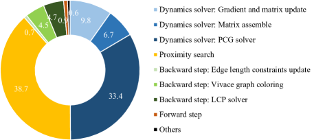
Figure 14. Breakdown analysis. We visualize a typical breakdown of the cost spent in each stage on the bow knot example. As shown in this figure, the PCG solves and the proximity search are the two most expensive parts in our simulator.

7. Results and Discussions

We test our simulator on an Intel Core i5-7500 3.4GHz CPU and an NVIDIA GeForce GTX 2080 Ti GPU. Table 1 summarizes the statistics and performances of our examples, and Table 2 provides major parameters and their default values used in our algorithm. Most results are computed with the default $\delta=1$mm. Specifically, $\delta=0.5$mm is used for the knotting examples in Fig. 1 and $\delta=0.2$mm is used for the hair example in Fig. 3. Our examples include both scenes of common benchmarks with complex collisions (Figs. 1 and 12), and virtual garments of multiple layers dressed on human bodies (Fig. 21). Related animation sequences are provided in the supplemental video. In general, the cost for handling contacts depends on the number of colliding elements and the number of steps, which are in essence determined by the time step and the shape complexity. By default, the step number limit $L$ is set to $512$ when $\Delta t=1/100$s, and $2,048$ when $\Delta t=1/20$s. In practice, our method typically converges in condition of $\|\mathbf{r}\|_{\infty}$ less than 64 steps, far before reaching the step number limit $L$ as Table 1 shows.

Table 2. Parameters and their default values.

Symbol	Meaning	Value
$L$	The limit on the number of steps	512 to 2,048
$\epsilon$	The termination threshold	0.0001
$D^{\min}$	The proximity search lower bound	2mm
$D^{\max}$	The proximity search upper bound	4mm
$\delta$	The constraint activation threshold	1mm
$\sigma$	The violation ratio limit	1.1
$\gamma$	The damping factor on movement	0.9

7.1. Breakdown Analysis

Fig. 14 provides a breakdown of the computational cost spent in the bow knot example (Fig. 1). It shows that PCG solves and proximity search are the two most expensive components in our simulator. In comparison, the actual cost spent by the forward step and backward step is much lower, i.e., occupying only 10.8 percent of the total cost. It suggests that our simulator still has a large space for performance improvement and it should benefit greatly from faster linear solvers and proximity search algorithms in the future.

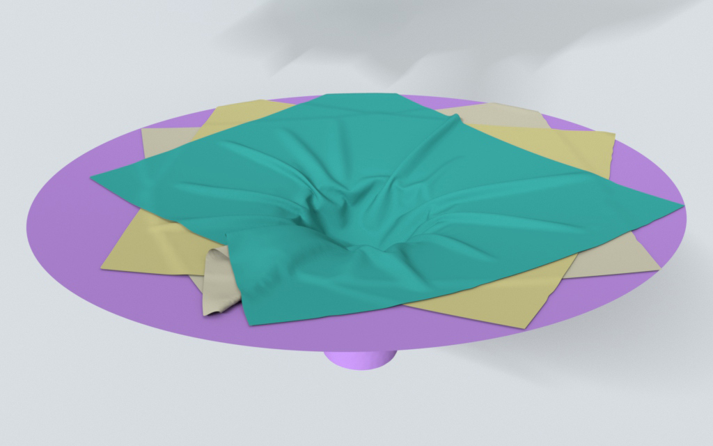
(a) $\Delta t$=1/20s

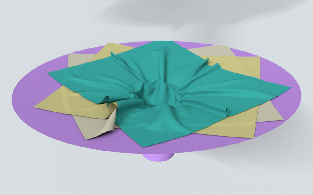
(b) $\Delta t$=1/40s

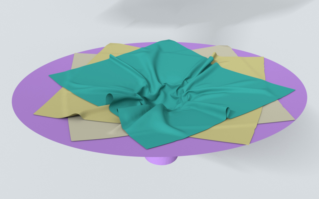
(c) $\Delta t$=1/80s

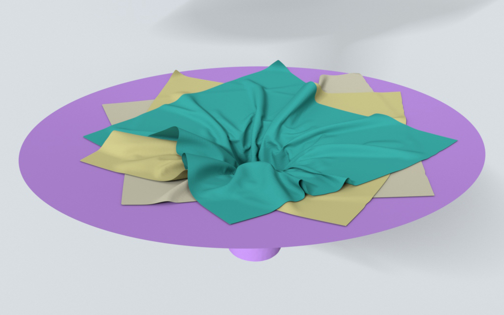
(d) $\Delta t$=1/160s

Figure 15. Funnel. We simulate this example with different time step sizes. While our method can reliably process collisions at a very large time step, i.e., $\Delta t=1/20$s, we suggest using a smaller time step in practice for more accurate results with less artificial damping.

7.2. Sensitivity to Time Steps

While our method is safe and robust regardless of time step size, its performance per step drops as the time step increases. Fundamentally, this is due to more severe collision cases and more steps needed for the method to converge. In our experiment, we test the funnel example with four time steps: $\Delta t$=1/160s, $\Delta t$=1/80s, $\Delta t$=1/40s and $\Delta t$=1/20s, and we intentionally set $L$=65,536 so that we can know how many steps are needed for convergence. Fig. 15 compares our simulation results in this example and Table 1 provides their performances. From the performance perspective only, it is beneficial to use a larger time step to reduce the computational overhead associated with every time step. However, due to the existence of artificial damping, we should avoid very large time steps in actual applications.

7.3. Comparison to Existing Collision Handling Methods

As we argued above, the major problems of existing collision handling algorithms (Harmon et al., 2008; Narain et al., 2012; Tang et al., 2016, 2018b, 2018a; Li et al., 2020b) for the step-and-project method are their linear path assumption and inappropriate measurement of distance. Such issues are exposed in a simple example as shown in Fig. 16: we initialize the angular velocity of various magnitudes in plane, leading to different targets $\mathbf{y}^{[k+1]}$ with increasing spin angles after the dynamics step. As the spin angle increases, the actual trajectory of every vertex should be close to a helix passing through the five-faces-spike obstacle surface under gravity. Therefore, restricting to a linear path can make the algorithm difficult to find a valid path not colliding with the obstacle, which might become impossible for complex shapes. Fig. 16(e) demonstrates such an increasing difficulty: as $\theta$ increases, the inelastic impact zone method (Harmon et al., 2008) implemented in ARCSim (Narain et al., 2012) requires drastically increasing cost to find a valid path. We note that when $\theta$ reaches $125^{\circ}$, the program cannot converge in two hours no matter how we tune the parameters.

Instead, our method runs inexpensive forward steps to form a piecewise linear path safely. In fact, this not only avoids expensive CCD tests, but also greatly increases the chances to find a valid path by exploring a larger space compared to a single line segment. Furthermore, with the help of the additional edge length constraints, the over-stretched artifacts arising from long-distance projection are pleasingly removed. Consequently, our two-way method can robustly remove all intersections along the path and reach a plausible and collision-free result (see Fig. 17 and the supplemental video) at a low cost (Fig. 16(e)).

Due to the high quality of the outputs in our two-way collision handling module, the entire simulation also suffers from much fewer nonphysical artifacts than the existing methods as Fig. 18 and the supplemental video demonstrate. Specifically, ARCSim (Narain et al., 2012) and CAMA (Tang et al., 2016), these two implementations of non-rigid impact zone optimization (Harmon et al., 2008) are involved for evaluations, where obvious nonphysical artifacts are observed. Note that other implementations, such as (Harmon et al., 2008; Tang et al., 2018b; Li et al., 2020b; Tang et al., 2018a), should suffer from similar artifacts due to the inheritance of methodology as we introduced above, though with different performances. In detail, to control the comparison targets, starting with the same $\mathbf{x}^{0}$, we run one Newton iteration by the same implementation and parameter setting to get $\mathbf{y}^{[1]}$ from a starting point $\mathbf{x}^{[0]}$ (the same as $\mathbf{x}^{t}$) in the dynamics step, and then we save the $\mathbf{x}^{[0]}$—$\mathbf{y}^{[1]}$ pair as OBJ files and “feed” this pair to different collision handling methods right afterwards to get different $\mathbf{x}^{[1]}$ (the same as $\mathbf{x}^{t+1}$), and then we save $\mathbf{x}^{[1]}$ as a OBJ file to “feed” back to the dynamics step, update velocity as $\mathbf{v}^{t+1}=\frac{\mathbf{x}^{t+1}-\mathbf{x}^{t}}{\Delta t}=\frac{\mathbf{x}^{[1]}-\mathbf{x}^{[0]}}{\Delta t}$ (we only have $k=0$ because we only run one Newton iteration) and start a new time step. This helps us keep the entire pipeline with all components the same, except for swapping in different projection methods to be compared. Note that the input and output of these methods have the same form as ours, a given $\mathbf{x}^{[k]}$—$\mathbf{y}^{[k+1]}$ pair and a resulted $\mathbf{x}^{[k+1]}$.

Theoretically, we note that there exists one class of inequality-constrained nonlinear optimization methods working in a step-and-project manner, the projected gradient (Newton) method   (Conn et al., 1988; Lin and Moré, 1999; Jorge and Stephen, 2006) . Given a gradient direction or Newton direction (a linear path of high dimension), the projection operator progressively projects the state into feasible domain and forms a piecewise linear path of high dimension. The piecewise linear property is important for incorporating appropriate global convergence techniques into it, such as computing the generalized Cauchy point. Compared with existing collision handling methods in the step-and-project pipeline, our method works in a similar way to it and the formed constrained path shares the common pieciewise-linear property with it. Therefore, we leave it to extend our method into an intact projected gradient (Newton) method for collision handling as future work.

(a) $\mathbf{x}^{[k]}$ and $\mathbf{y}^{[k+1]}$ when $\theta=0^{\circ}$

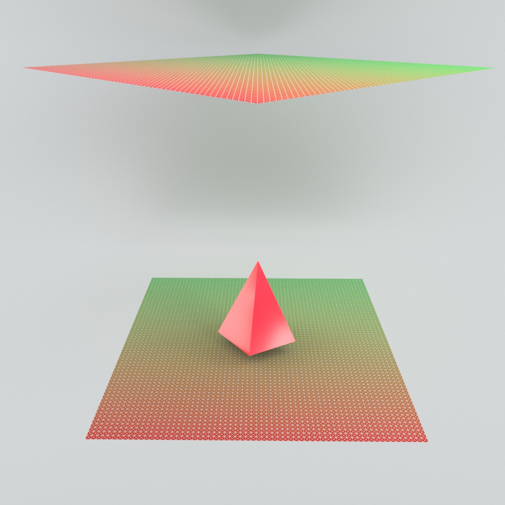
(b) $\mathbf{x}^{[k]}$ and $\mathbf{y}^{[k+1]}$ when $\theta=45^{\circ}$

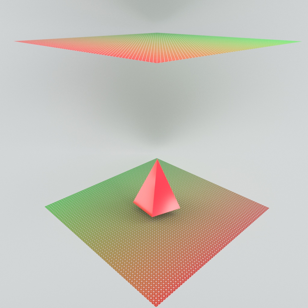
(c) $\mathbf{x}^{[k]}$ and $\mathbf{y}^{[k+1]}$ when $\theta=90^{\circ}$

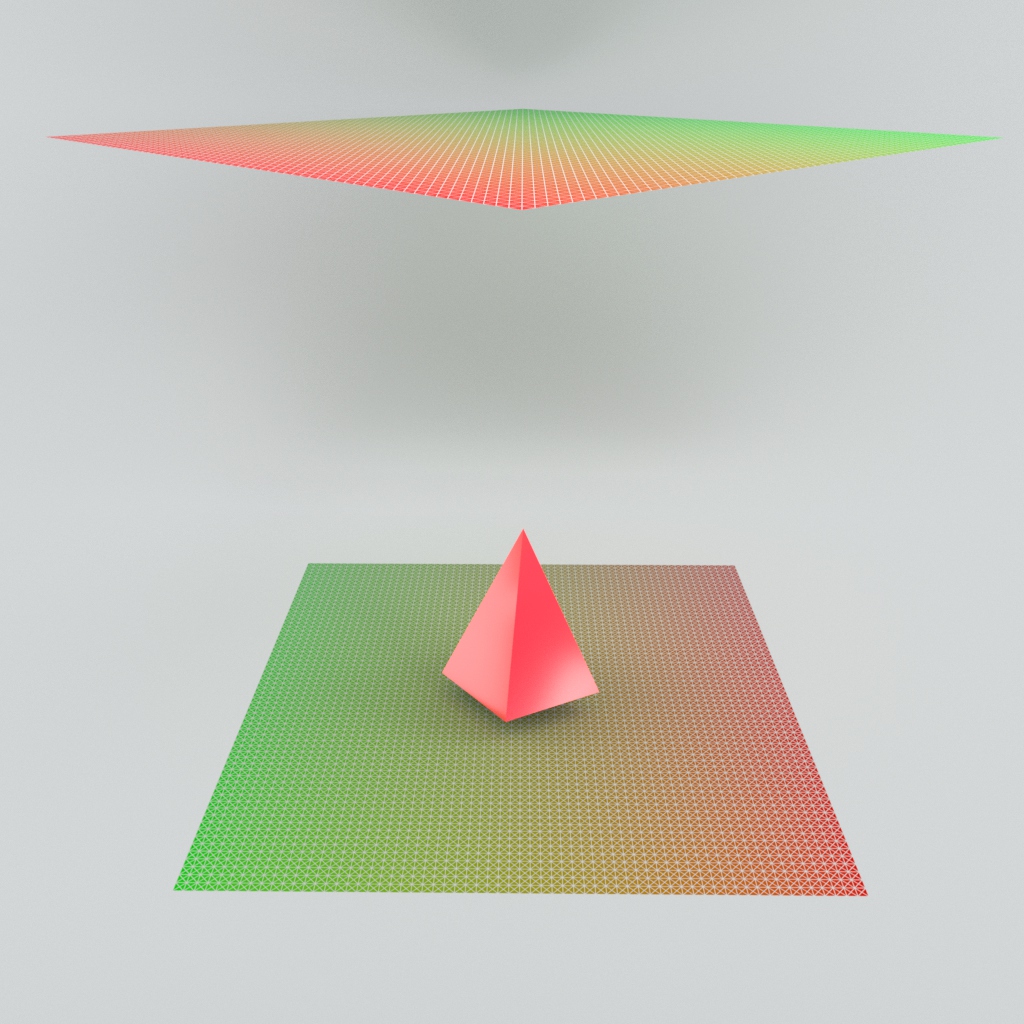
(d) $\mathbf{x}^{[k]}$ and $\mathbf{y}^{[k+1]}$ when $\theta=135^{\circ}$

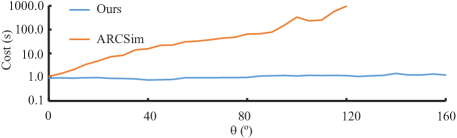
(e) Time cost comparison with ARCSim (Narain et al., 2012)

Figure 16. Spinning cloth patch. From (a) to (d), the spin angle $\theta$ between $\mathbf{x}^{[k]}$ and $\mathbf{y}^{[k+1]}$ is increasing, and we use the color ramp to illustrate region correspondence. As $\theta$ increases, ARCSim is getting harder to find a valid path, while our method is almost free of such drastic growth in time cost (Fig. (e)).

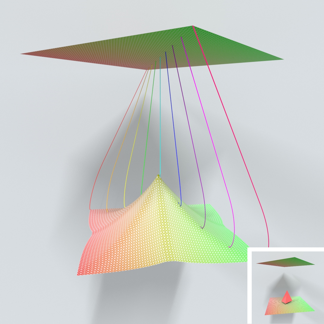
(a) $\mathbf{x}^{[k]}$ and $\mathbf{x}^{[k+1]}$ by our method when   $\theta=45^{\circ}$

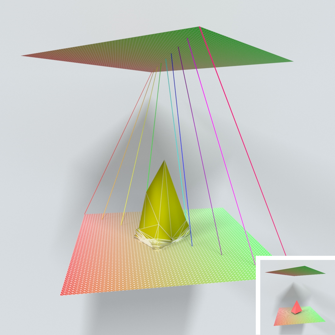
(b) $\mathbf{x}^{[k]}$ and $\mathbf{x}^{[k+1]}$ by ARCSim when   $\theta=45^{\circ}$

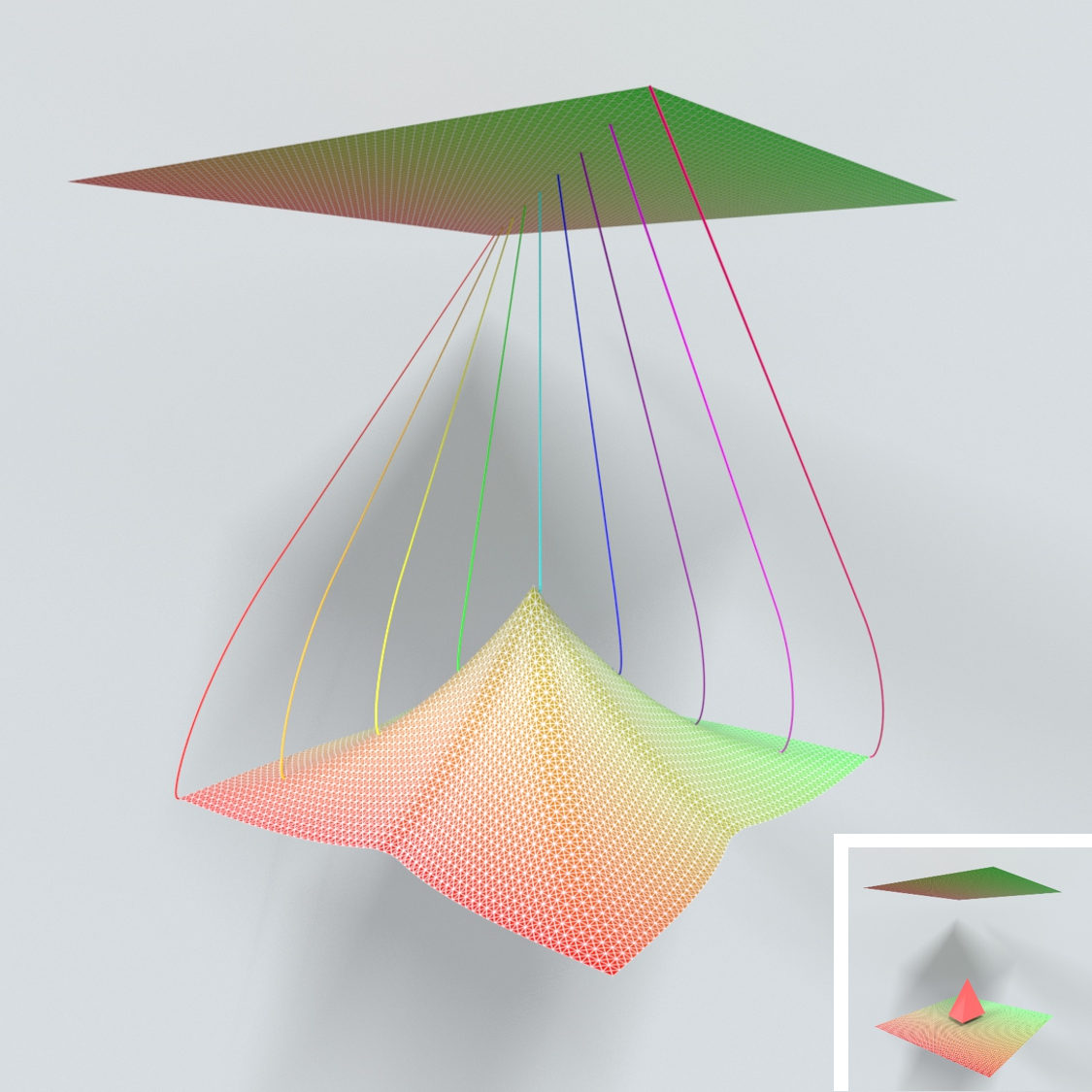
(c) $\mathbf{x}^{[k]}$ and $\mathbf{x}^{[k+1]}$ by our method when   $\theta=90^{\circ}$

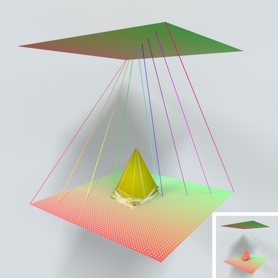
(d) $\mathbf{x}^{[k]}$ and $\mathbf{x}^{[k+1]}$ by ARCSim when   $\theta=90^{\circ}$

Figure 17. Trajectories avoiding collisions. Here we track the trajectories of nine vertices on one diagonal of the cloth patch, which are progressively generated by our two-way approach. Compared to the impact zone optimization implemented by ARCSim (Narain et al., 2012), our method allows a curved path from $\mathbf{x}^{[k]}$ to $\mathbf{x}^{[k+1]}$ to resolve collisions where neither intersections nor spuriously stretched elements can appear, while restricting to a linear path may fail to find a faithful solution at a reasonable cost.

(a) CAMA (Tang et al., 2016)

(b) ARCSim (Narain et al., 2012)

(c) Our method

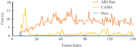
(d) Time cost comparison

Figure 18. Robustness to large time steps. A piece of cloth falling on a sharp cone is simulated with a large time step ($\Delta t=1/10$s). Compared with existing impact zone methods such as (Tang et al., 2016; Narain et al., 2012), our result has much less visual artifacts over time, even with much less computational cost.

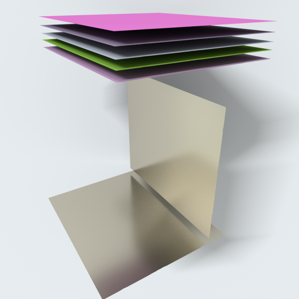
(a) The initial state

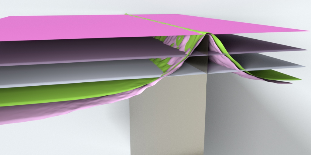
(b) Before repair

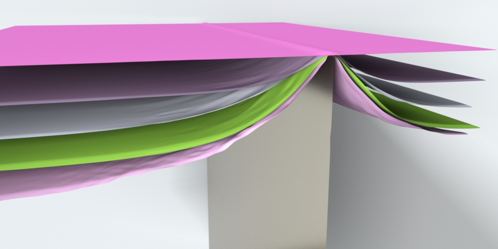
(c) After repair

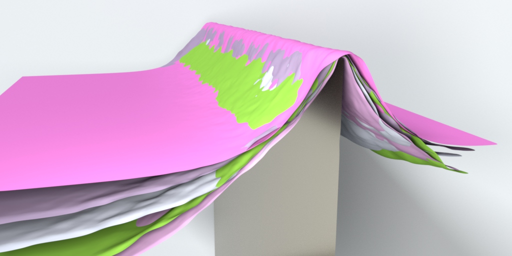
(d) Before repair

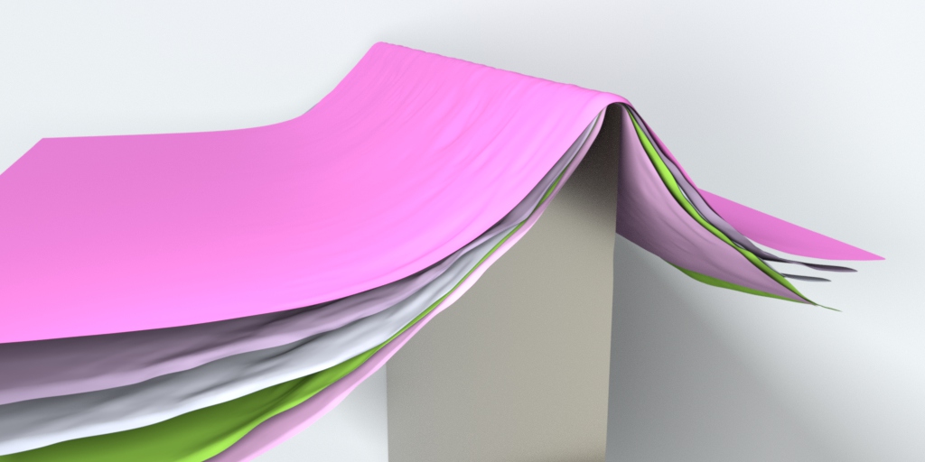
(e) After repair

Figure 19. Cloth and blade colliding. In this example, five square cloth patches drop onto a sharp metal blade, then drape, slide and stack under gravity. Our method can robustly project seriously penetrated frames ((b) and (d)) to intersection-free states ((c) and (e)).

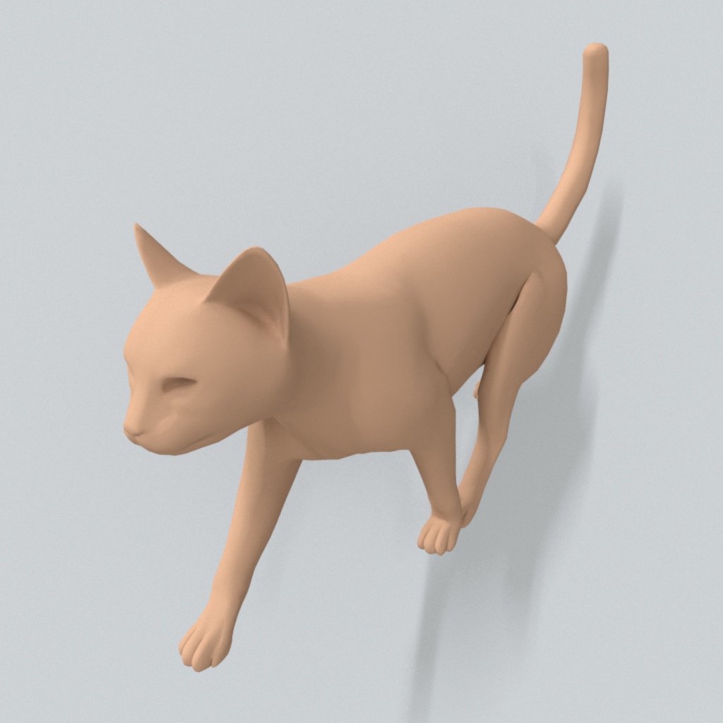
(a) The initial state

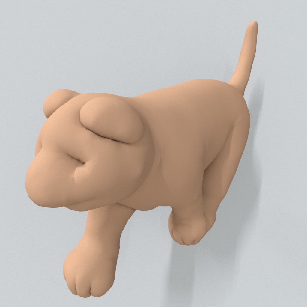
(b) The positive flow

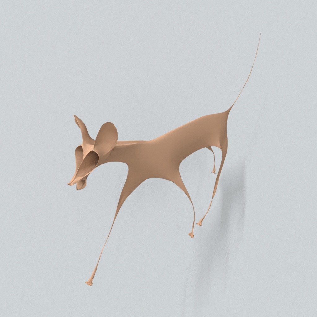
(c) The negative flow

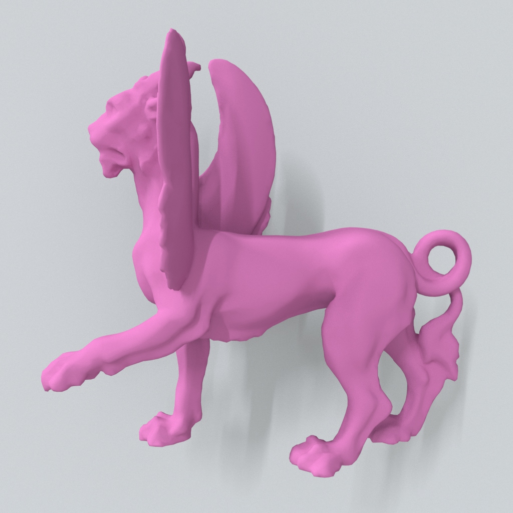
(d) The initial state

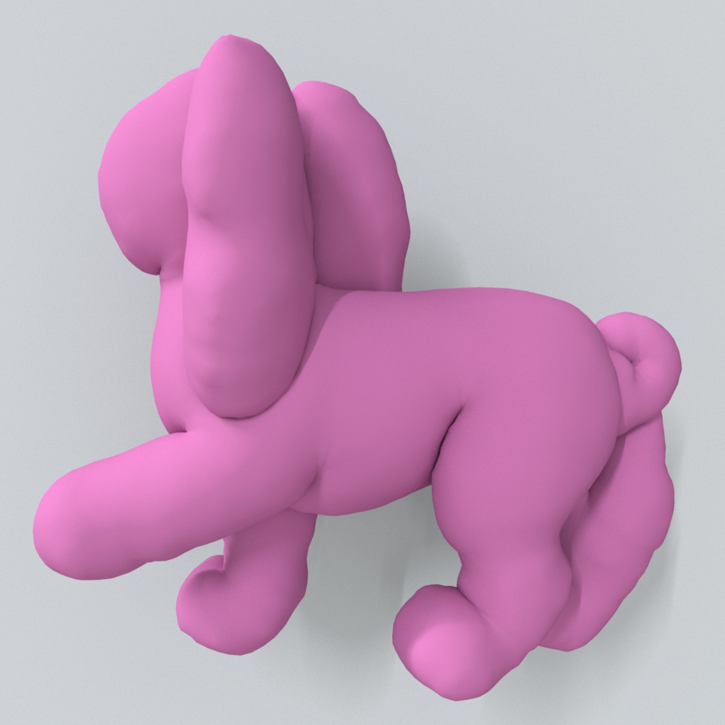
(e) The positive flow

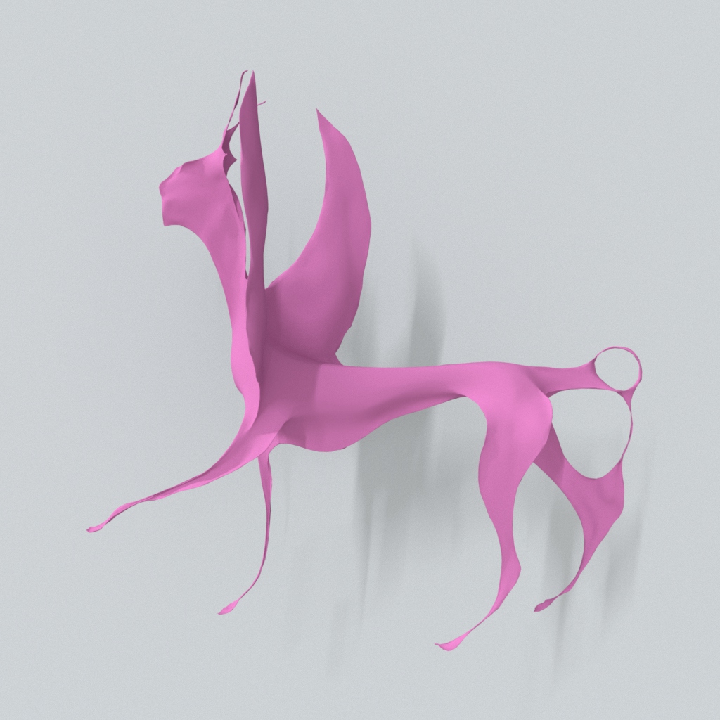
(f) The negative flow

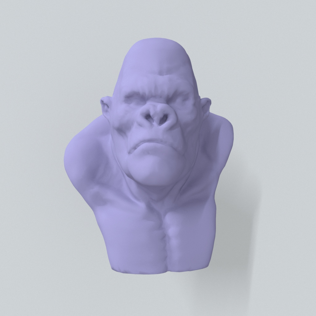
(g) The initial state

(h) The positive flow

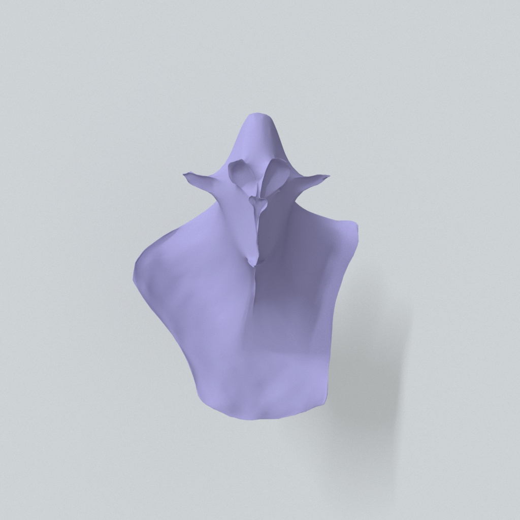
(i) The negative flow

Figure 20. Globally injective normal flow. Our method can be also applied to enforce global injectivity in both positive and negative normal flows.

7.4. Geometry Processing

Since our method works as a standalone module to resolve collisions, it can be seamlessly integrated into geometry processing applications for intersection-free results. For instance, our method can fix seriously self-intersecting animation frames robustly, such as the blade example shown in Fig. 19. We can also apply our method to enforce global injectivity in normal flow computations, such as the ones shown in Fig. 20.

For the globally injective normal flow application, we first compute ${\mathbf{y}}^{[k+1]}$ as below:

(19) $$\left\{\begin{array}[]{l}{\mathbf{y}}_{0}^{[k+1]}={\mathbf{x}}^{[k]}\pm\beta{\mathbf{n}}^{[k]},\\ {\mathbf{y}}_{i+1}^{[k+1]}(v)={\mathbf{y}}_{i}^{[k+1]}(v)+\alpha\mathop{}\!\mathbin{\bigtriangleup}{\mathbf{y}}_{i}^{[k+1]}(v),\\ {\mathbf{y}}^{[k+1]}={\mathbf{y}}_{3}^{[k+1]},\end{array}\right.$$

in which $\mathbf{n}^{[k]}$ is the normal vector field of the surface at $\mathbf{x}^{[k]}$, $\beta$ is the flow speed, $\alpha$ is the smoothing intensity and $\mathop{}\!\mathbin{\bigtriangleup}$ is the cotangent-formed (Pinkall and Polthier, 1993; Desbrun et al., 1999; Meyer et al., 2003) discretization of the Laplace-Beltrami operator. We smooth in a simple Jacobi fashion for each vertex $v$ and fix the smoothing iterations be three to get $\mathbf{y}^{[k+1]}$. Then we run our two-way method for guaranteeing global injectivity. Finally, we get highly similar results compared with (Fang et al., 2021), on all examples from their benchmarks as shown in Fig. 20 within less than $1$s.

8. Limitations and future works

While the experiments demonstrate the efficiency, robustness and good quality of our collision handling algorithm, there is no guarantee of a globally convergent approximate solution to Eq. (1). In fact, compared to the recently developed incremental potential contact (IPC) method (Li et al., 2021), all step-and-project methods seem to lack theoretical guarantee of global convergence in exchange for numerical efficiency. Therefore, we do not compare our method with IPC directly in terms of performance for fairness reasons. Although finding a convergent solution to Eq. (1) could be over-demanding and unnecessary for a faithful simulation in graphics, analyzing the compromise made by step-and-project methods and further improving its convergence is definitely a valuable future work. Besides, our method does not consider friction modeling yet. Now it simply imitates frictional effects using an additional velocity filter. If trying to reproduce more realistic frictional contacts, the method should handle collisions and frictions jointly instead. Finally, we are interested in implementing our method on distributed systems consisting of multiple GPUs for real-time performance on large-scale scenes. To sufficiently exploit the power of distributed systems, we need to carefully study the communications between tasks, processes and threads, and thus design effective policy for parallelization and synchronization.

References

- (1)
- Ainsley et al. (2012) Samantha Ainsley, Etienne Vouga, Eitan Grinspun, and Rasmus Tamstorf. 2012. Speculative Parallel Asynchronous Contact Mechanics. ACM Trans. Graph. 31, 6, Article 151 (nov 2012), 8 pages.
- Andrews et al. (2022) Sheldon Andrews, Kenny Erleben, and Zachary Ferguson. 2022. Contact and friction simulation for computer graphics. In ACM SIGGRAPH 2022 Courses. 1–172.
- Baraff et al. (2003) David Baraff, Andrew Witkin, and Michael Kass. 2003. Untangling Cloth. ACM Trans. Graph. 22, 3 (jul 2003), 862–870.
- Barbič and James (2010) Jernej Barbič and Doug L. James. 2010. Subspace Self-Collision Culling. In ACM SIGGRAPH 2010 Papers (SIGGRAPH ’10). Association for Computing Machinery, New York, NY, USA, Article 81, 9 pages.
- Bergou et al. (2006) Miklos Bergou, Max Wardetzky, David Harmon, Denis Zorin, and Eitan Grinspun. 2006. A Quadratic Bending Model for Inextensible Surfaces. In Proceedings of the Fourth Eurographics Symposium on Geometry Processing (SGP ’06). Eurographics Association, Goslar, DEU, 227–230.
- Bertails-Descoubes et al. (2011) Florence Bertails-Descoubes, Florent Cadoux, Gilles Daviet, and Vincent Acary. 2011. A Nonsmooth Newton Solver for Capturing Exact Coulomb Friction in Fiber Assemblies. ACM Trans. Graph. 30, 1, Article 6 (feb 2011), 14 pages.
- Bridson et al. (2002) Robert Bridson, Ronald Fedkiw, and John Anderson. 2002. Robust Treatment of Collisions, Contact and Friction for Cloth Animation. ACM Trans. Graph. 21, 3 (jul 2002), 594–603.
- Bridson et al. (2005) R. Bridson, S. Marino, and R. Fedkiw. 2005. Simulation of Clothing with Folds and Wrinkles. In ACM SIGGRAPH 2005 Courses (SIGGRAPH ’05). Association for Computing Machinery, New York, NY, USA, 28–36.
- Chen et al. (2022) Yunuo Chen, Minchen Li, Lei Lan, Hao Su, Yin Yang, and Chenfanfu Jiang. 2022. A unified newton barrier method for multibody dynamics. ACM Transactions on Graphics (TOG) 41, 4 (2022), 1–14.
- Choi and Ko (2002) Kwang-Jin Choi and Hyeong-Seok Ko. 2002. Stable but Responsive Cloth. ACM Trans. Graph. 21, 3 (jul 2002), 604–611.
- Conn et al. (1988) Andrew R Conn, Nicholas IM Gould, and Ph L Toint. 1988. Global convergence of a class of trust region algorithms for optimization with simple bounds. SIAM journal on numerical analysis 25, 2 (1988), 433–460.
- Daviet (2020) Gilles Daviet. 2020. Simple and Scalable Frictional Contacts for Thin Nodal Objects. ACM Trans. Graph. 39, 4, Article 61 (jul 2020), 16 pages.
- Desbrun et al. (1999) Mathieu Desbrun, Mark Meyer, Peter Schröder, and Alan H. Barr. 1999. Implicit Fairing of Irregular Meshes Using Diffusion and Curvature Flow. In Proceedings of the 26th Annual Conference on Computer Graphics and Interactive Techniques (SIGGRAPH ’99). ACM Press/Addison-Wesley Publishing Co., USA, 317–324.
- Erleben (2013) Kenny Erleben. 2013. Numerical Methods for Linear Complementarity Problems in Physics-Based Animation. In ACM SIGGRAPH 2013 Courses (SIGGRAPH ’13). Association for Computing Machinery, New York, NY, USA, Article 8, 42 pages.
- Etzmuß et al. (2003) Olaf Etzmuß, Michael Keckeisen, and Wolfgang Straßer. 2003. A fast finite element solution for cloth modelling. In 11th Pacific Conference onComputer Graphics and Applications, 2003. Proceedings. IEEE, 244–251.
- Fang et al. (2021) Yu Fang, Minchen Li, Chenfanfu Jiang, and Danny M. Kaufman. 2021. Guaranteed Globally Injective 3D Deformation Processing. ACM Trans. Graph. 40, 4, Article 75 (jul 2021), 13 pages.
- Fratarcangeli et al. (2016) Marco Fratarcangeli, Valentina Tibaldo, and Fabio Pellacini. 2016. Vivace: A Practical Gauss-Seidel Method for Stable Soft Body Dynamics. ACM Trans. Graph. 35, 6, Article 214 (nov 2016), 9 pages.
- Gao* et al. (2018) Ming Gao*, Xinlei Wang*, Kui Wu*, Andre Pradhana, Eftychios Sifakis, Cem Yuksel, and Chenfanfu Jiang. 2018. GPU Optimization of Material Point Methods. ACM Transactions on Graphics (Proceedings of SIGGRAPH ASIA 2018) 37, 6 (2018). (*Joint First Authors).
- Grinspun et al. (2003) Eitan Grinspun, Anil N Hirani, Mathieu Desbrun, and Peter Schröder. 2003. Discrete shells. In Proceedings of the 2003 ACM SIGGRAPH/Eurographics symposium on Computer animation. 62–67.
- Harmon et al. (2009) David Harmon, Etienne Vouga, Breannan Smith, Rasmus Tamstorf, and Eitan Grinspun. 2009. Asynchronous Contact Mechanics. ACM Trans. Graph. 28, 3, Article 87 (jul 2009), 12 pages.
- Harmon et al. (2008) David Harmon, Etienne Vouga, Rasmus Tamstorf, and Eitan Grinspun. 2008. Robust Treatment of Simultaneous Collisions. ACM Trans. Graph. 27, 3 (aug 2008), 1–4.
- Harmon et al. (2011) David Harmon, Qingnan Zhou, and Denis Zorin. 2011. Asynchronous Integration with Phantom Meshes. In Proceedings of the 2011 ACM SIGGRAPH/Eurographics Symposium on Computer Animation (SCA ’11). Association for Computing Machinery, New York, NY, USA, 247–256.
- Jorge and Stephen (2006) Nocedal Jorge and J Wright Stephen. 2006. Numerical optimization.
- Kane et al. (1999) Couro Kane, Eduardo A Repetto, Michael Ortiz, and Jerrold E Marsden. 1999. Finite element analysis of nonsmooth contact. Computer methods in applied mechanics and engineering 180, 1-2 (1999), 1–26.
- Lan et al. (2022) Lei Lan, Guanqun Ma, Yin Yang, Changxi Zheng, Minchen Li, and Chenfanfu Jiang. 2022. Penetration-Free Projective Dynamics on the GPU. ACM Trans. Graph. 41, 4, Article 69 (jul 2022), 16 pages.
- Lauterbach et al. (2010) Christian Lauterbach, Qi Mo, and Dinesh Manocha. 2010. gProximity: Hierarchical GPU-Based Operations for Collision and Distance Queries. In Proceedings of Eurographics, Vol. 29. 419–428.
- Li et al. (2020b) Cheng Li, Min Tang, Ruofeng Tong, Ming Cai, Jieyi Zhao, and Dinesh Manocha. 2020b. P-Cloth: Interactive Complex Cloth Simulation on Multi-GPU Systems Using Dynamic Matrix Assembly and Pipelined Implicit Integrators. ACM Trans. Graph. 39, 6, Article 180 (nov 2020), 15 pages.
- Li et al. (2020a) Minchen Li, Zachary Ferguson, Teseo Schneider, Timothy Langlois, Denis Zorin, Daniele Panozzo, Chenfanfu Jiang, and Danny M. Kaufman. 2020a. Incremental Potential Contact: Intersection-and Inversion-Free, Large-Deformation Dynamics. ACM Trans. Graph. 39, 4, Article 49 (jul 2020), 20 pages.
- Li et al. (2021) Minchen Li, Danny M. Kaufman, and Chenfanfu Jiang. 2021. Codimensional Incremental Potential Contact. ACM Trans. Graph. 40, 4, Article 170 (jul 2021), 24 pages.
- Lin and Moré (1999) Chih-Jen Lin and Jorge J Moré. 1999. Newton’s method for large bound-constrained optimization problems. SIAM Journal on Optimization 9, 4 (1999), 1100–1127.
- Ly et al. (2020) Mickaël Ly, Jean Jouve, Laurence Boissieux, and Florence Bertails-Descoubes. 2020. Projective Dynamics with Dry Frictional Contact. ACM Trans. Graph. 39, 4, Article 57 (jul 2020), 8 pages.
- Macklin et al. (2019) Miles Macklin, Kenny Erleben, Matthias Müller, Nuttapong Chentanez, Stefan Jeschke, and Viktor Makoviychuk. 2019. Non-Smooth Newton Methods for Deformable Multi-Body Dynamics. ACM Trans. Graph. 38, 5, Article 140 (oct 2019), 20 pages.
- Macklin and Muller (2021) Miles Macklin and Matthias Muller. 2021. A Constraint-Based Formulation of Stable Neo-Hookean Materials. In Motion, Interaction and Games (MIG ’21). Association for Computing Machinery, New York, NY, USA, Article 12, 7 pages.
- Martin et al. (2011) Sebastian Martin, Bernhard Thomaszewski, Eitan Grinspun, and Markus Gross. 2011. Example-Based Elastic Materials. In ACM SIGGRAPH 2011 Papers (SIGGRAPH ’11). Association for Computing Machinery, New York, NY, USA, Article 72, 8 pages.
- Meyer et al. (2003) Mark Meyer, Mathieu Desbrun, Peter Schröder, and Alan H Barr. 2003. Discrete differential-geometry operators for triangulated 2-manifolds. In Visualization and mathematics III. Springer, 35–57.
- Mirtich (2000) Brian Mirtich. 2000. Timewarp Rigid Body Simulation. In Proceedings of the 27th Annual Conference on Computer Graphics and Interactive Techniques (SIGGRAPH ’00). ACM Press/Addison-Wesley Publishing Co., USA, 193–200.
- Mirtich and Canny (1995) Brian Mirtich and John Canny. 1995. Impulse-Based Dynamic Simulation. In Proceedings of the Workshop on Algorithmic Foundations of Robotics (WAFR). A. K. Peters, Ltd., USA, 407–418.
- Müller (2008) Matthias Müller. 2008. Hierarchical Position Based Dynamics. In Proceedings of Virtual Reality Interactions and Physical Simulations. Grenoble.
- Müller et al. (2015) Matthias Müller, Nuttapong Chentanez, Tae-Yong Kim, and Miles Macklin. 2015. Air meshes for robust collision handling. ACM Transactions on Graphics (TOG) 34, 4 (2015), 1–9.
- Narain et al. (2012) Rahul Narain, Armin Samii, and James F. O’Brien. 2012. Adaptive Anisotropic Remeshing for Cloth Simulation. ACM Trans. Graph. 31, 6, Article 152 (nov 2012), 10 pages.
- Pabst et al. (2010) Simon Pabst, Artur Koch, and Wolfgang Straßer. 2010. Fast and Scalable CPU/GPU Collision Detection for Rigid and Deformable Surfaces. Comput. Graph. Forum 29, 5 (2010), 1605–1612.
- Pinkall and Polthier (1993) Ulrich Pinkall and Konrad Polthier. 1993. Computing discrete minimal surfaces and their conjugates. Experimental mathematics 2, 1 (1993), 15–36.
- Provot (1997) Xavier Provot. 1997. Collision and Self-Collision Handling in Cloth Model Dedicated to Design Garments. In Computer Animation and Simulation. 177–189.
- Sifakis et al. (2008) Eftychios Sifakis, Sebastian Marino, and Joseph Teran. 2008. Globally Coupled Collision Handling Using Volume Preserving Impulses. In Proceedings of the 2008 ACM SIGGRAPH/Eurographics Symposium on Computer Animation (SCA ’08). Eurographics Association, Goslar, DEU, 147–153.
- Smith et al. (2019) Breannan Smith, Fernando De Goes, and Theodore Kim. 2019. Analytic eigensystems for isotropic distortion energies. ACM Transactions on Graphics (TOG) 38, 1 (2019), 1–15.
- Smith and Schaefer (2015) Jason Smith and Scott Schaefer. 2015. Bijective Parameterization with Free Boundaries. ACM Trans. Graph. 34, 4, Article 70 (jul 2015), 9 pages.
- Stam (2009) Jos Stam. 2009. Nucleus: Towards a Unified Dynamics Solver for Computer Graphics. In 11th IEEE International Conference on Computer-Aided Design and Computer Graphics.
- Tang et al. (2010) Min Tang, Young J. Kim, and Dinesh Manocha. 2010. Continuous Collision Detection for Non-Rigid Contact Computations using Local Advancement. In Proceedings of ICRA. 4016–4021.
- Tang et al. (2018a) Min Tang, Zhongyuan Liu, Ruofeng Tong, and Dinesh Manocha. 2018a. PSCC: Parallel Self-Collision Culling with Spatial Hashing on GPUs. Proc. ACM Comput. Graph. Interact. Tech. 1, 1, Article 18 (jul 2018), 18 pages.
- Tang et al. (2011a) Min Tang, Dinesh Manocha, Jiang Lin, and Ruofeng Tong. 2011a. Collision-streams: Fast GPU-based collision detection for deformable models. In Symposium on interactive 3D graphics and games. 63–70.
- Tang et al. (2011b) Min Tang, Dinesh Manocha, Sung-Eui Yoon, Peng Du, Jae-Pil Heo, and Ruo-Feng Tong. 2011b. VolCCD: Fast Continuous Collision Culling between Deforming Volume Meshes. ACM Trans. Graph. 30, 5, Article 111 (oct 2011), 15 pages.
- Tang et al. (2014) Min Tang, Ruofeng Tong, Zhendong Wang, and Dinesh Manocha. 2014. Fast and Exact Continuous Collision Detection with Bernstein Sign Classification. ACM Trans. Graph. 33, 6, Article 186 (nov 2014), 8 pages.
- Tang et al. (2016) Min Tang, Huamin Wang, Le Tang, Ruofeng Tong, and Dinesh Manocha. 2016. CAMA: Contact-Aware Matrix Assembly with Unified Collision Handling for GPU-Based Cloth Simulation. Comput. Graph. Forum (Eurographics) 35, 2 (May 2016), 511–521.
- Tang et al. (2018b) Min Tang, tongtong wang, Zhongyuan Liu, Ruofeng Tong, and Dinesh Manocha. 2018b. I-Cloth: Incremental Collision Handling for GPU-Based Interactive Cloth Simulation. ACM Trans. Graph. 37, 6, Article 204 (dec 2018), 10 pages.
- Teran et al. (2005) Joseph Teran, Eftychios Sifakis, Geoffrey Irving, and Ronald Fedkiw. 2005. Robust quasistatic finite elements and flesh simulation. In Proceedings of the 2005 ACM SIGGRAPH/Eurographics symposium on Computer animation. 181–190.
- Teschner et al. (2003) Matthias Teschner, Bruno Heidelberger, Matthias Müller, Danat Pomerantes, and Markus H Gross. 2003. Optimized Spatial Hashing for Collision Detection of Deformable Objects. In Proceedings of Vision, Modeling, Visualization, Vol. 3. 47–54.
- Thomaszewski et al. (2008) Bernhard Thomaszewski, Simon Pabst, and Wolfgang Straßer. 2008. Asynchronous Cloth Simulation. In Proceedings of Computer Graphics International.
- Verschoor and Jalba (2019) Mickeal Verschoor and Andrei C. Jalba. 2019. Efficient and Accurate Collision Response for Elastically Deformable Models. ACM Trans. Graph. 38, 2, Article 17 (mar 2019), 20 pages.
- Volino and Magnenat-Thalmann (2006) Pascal Volino and Nadia Magnenat-Thalmann. 2006. Resolving Surface Collisions through Intersection Contour Minimization. In ACM SIGGRAPH 2006 Papers (SIGGRAPH ’06). Association for Computing Machinery, New York, NY, USA, 1154–1159.
- Von Herzen et al. (1990) Brian Von Herzen, Alan H. Barr, and Harold R. Zatz. 1990. Geometric Collisions for Time-Dependent Parametric Surfaces. SIGGRAPH Comput. Graph. 24, 4 (sep 1990), 39–48.
- Wang et al. (2021) Bolun Wang, Zachary Ferguson, Teseo Schneider, Xin Jiang, Marco Attene, and Daniele Panozzo. 2021. A Large-scale Benchmark and an Inclusion-based Algorithm for Continuous Collision Detection. ACM Transactions on Graphics (TOG) 40, 5 (2021), 1–16.
- Wang (2014) Huamin Wang. 2014. Defending Continuous Collision Detection against Errors. ACM Trans. Graph. 33, 4, Article 122 (jul 2014), 10 pages.
- Wang (2015) Huamin Wang. 2015. A Chebyshev Semi-Iterative Approach for Accelerating Projective and Position-Based Dynamics. ACM Trans. Graph. 34, 6, Article 246 (oct 2015), 9 pages.
- Wang and Yang (2016) Huamin Wang and Yin Yang. 2016. Descent Methods for Elastic Body Simulation on the GPU. ACM Trans. Graph. 35, 6, Article 212 (nov 2016), 10 pages.
- Wang et al. (2017) Tongtong Wang, Zhihua Liu, Min Tang, Ruofeng Tong, and Dinesh Manocha. 2017. Efficient and Reliable Self-Collision Culling Using Unprojected Normal Cones. Comput. Graph. Forum (Eurographics) 36, 8 (2017), 487–498.
- Wicke et al. (2006) Martin Wicke, Hermes Lanker, and Markus Gross. 2006. Untangling Cloth with Boundaries. In Proceedings of Vision, Modeling, and Visualization. 349–356.
- Wu et al. (2020) Longhua Wu, Botao Wu, Yin Yang, and Huamin Wang. 2020. A Safe and Fast Repulsion Method for GPU-Based Cloth Self Collisions. ACM Trans. Graph. 40, 1, Article 5 (dec 2020), 18 pages.
- Yuksel (2022) Cem Yuksel. 2022. A Fast & Robust Solution for Cubic & Higher-Order Polynomials. In ACM SIGGRAPH 2022 Talks (SIGGRAPH ’22). Association for Computing Machinery, New York, NY, USA, Article 28, 2 pages.
- Zheng and James (2012) Changxi Zheng and Doug L. James. 2012. Energy-Based Self-Collision Culling for Arbitrary Mesh Deformations. ACM Trans. Graph. 31, 4, Article 98 (jul 2012), 12 pages.