Structured Mixture of Continuation-ratio Logits Models for Ordinal Regression

Abstract

We develop a nonparametric Bayesian modeling approach to ordinal regression based on priors placed directly on the discrete distribution of the ordinal responses. The prior probability models are built from a structured mixture of multinomial distributions. We leverage a continuation-ratio logits representation to formulate the mixture kernel, with mixture weights defined through the logit stick-breaking process that incorporates the covariates through a linear function. The implied regression functions for the response probabilities can be expressed as weighted sums of parametric regression functions, with covariate-dependent weights. Thus, the modeling approach achieves flexible ordinal regression relationships, avoiding linearity or additivity assumptions in the covariate effects. A key model feature is that the parameters for both the mixture kernel and the mixture weights can be associated with a continuation-ratio logits regression structure. Hence, an efficient and relatively easy to implement posterior simulation method can be designed, using Pólya-Gamma data augmentation. Moreover, the model is built from a conditional independence structure for category-specific parameters, which results in additional computational efficiency gains through partial parallel sampling. In addition to the general mixture structure, we study simplified model versions that incorporate covariate dependence only in the mixture kernel parameters or only in the mixture weights. For all proposed models, we discuss approaches to prior specification and develop Markov chain Monte Carlo methods for posterior simulation. The methodology is illustrated with several synthetic and real data examples.

Keywords: Bayesian nonparametric regression; Dependent Dirichlet process; Developmental toxicity studies; Logit stick-breaking prior; Markov chain Monte Carlo.

1 Introduction

Ordinal responses are widely encountered in many fields, including econometrics and the biomedical and social sciences, typically accompanied by covariate information. Hence, estimation and prediction of ordinal regression relationships remains a methodologically and practically relevant problem. A univariate ordinal response $Y$ with $C$ categories can be encoded as a $C$-dimensional binary vector $\mathbf{Y}$. The components of $\mathbf{Y}$ do not necessarily need to be binary, they may be extended to non-negative integers. We refer to data structures of these two types as the “standard” and “extended” setting, respectively. The modeling challenge for the ordinal regression problem involves capturing general regression relationships in the response probabilities (especially for moderate to large $C$), while at the same time appropriately accounting for the ordinal nature of the response distribution.

Traditionally, the standard ordinal regression problem is approached by treating the ordinal responses as a discretized version of latent continuous responses, which are usually assumed to be normally distributed resulting in popular ordinal probit models. For Bayesian inference, such data augmentation facilitates posterior simulation (Albert and Chib, 1993). However, probit models generally preclude a flexible analysis of probability response curves. For instance, covariate effects enter linearly and additively, and the normality assumption implies restrictions on the marginal response probabilities (e.g., Boes and Winkelmann, 2006). In general, parametric ordinal regression models sacrifice flexibility in the response distribution and/or the regression functions for the response probabilities.

To overcome such limitations, the earlier work in the Bayesian nonparametrics literature has explored semiparametric models, although most of this work has focused on the binary regression problem. Such methods relax parametric assumptions for the distribution of the latent variables (e.g., Basu and Chib, 2003) or for the regression function (e.g., Choudhuri et al., 2007). As a further extension, Chib and Greenberg (2010) modeled covariate effects additively by cubic splines, combined with a scale normal mixture for the latent responses, using the Dirichlet process (DP) prior (Ferguson, 1973) for the mixing distribution. More general DP mixture priors for the distribution of the latent continuous responses have been considered in Bao and Hanson (2015) and DeYoreo and Kottas (2018). The latter involves a fully nonparametric Bayesian method under the density regression framework, modeling the joint distribution of covariates and latent responses with a DP mixture of multivariate normals. We refer to DeYoreo and Kottas (2020) for a review of the joint response-covariate modeling approach with categorical variables. The density regression modeling framework is appealing with regard to the scope of ordinal regression inferences. However, it involves computationally intensive posterior simulation which does not scale with the number of covariates. Moreover, the modeling approach is not suitable for applications where the assumption of random covariates is not relevant. Finally, for a different nonparametric Bayesian modeling perspective, we refer to the recent work of Saarela et al. (2022) that extends monotonic multivariable regression to ordered categorical responses.

The “logits regression family” of parametric models (e.g., Agresti, 2012) offers an alternative approach to the ordinal regression problem, based on direct modeling of the response distribution. Of particular interest to our methodology are continuation-ratio logits models (Tutz, 1991). The continuation-ratio logits parameterization of the multinomial distribution implies a sequential mechanism, such that the ordinal response is determined through a sequence of binary outcomes. Starting from the lowest category, each binary outcome indicates whether the ordinal response belongs to that category or to one of the higher categories. The continuation-ratio logit for response category $j$ is the logit of the conditional probability of response $j$, given that the response is $j$ or higher. A key consequence is that, in a multinomial continuation-ratio logits regression model, the response distribution can be factorized into complete conditionals which are given by Binomial logistic regression models.

To our knowledge, continuation-ratio logits have not been explored for general Bayesian nonparametric methods for ordinal regression. For nominal regression, Linderman et al. (2015) discussed a semiparametric model that, under the mutlinomial response distribution, replaces the linear covariate effects within the continuation-ratio logits by Gaussian process priors. More relevant to our methodology is the dependent DP mixture model in Kottas and Fronczyk (2013), based on a trinomial kernel that builds from the continuation-ratio logits formulation. This modeling approach was developed specifically in the context of developmental toxicity studies, rather than for general ordinal regression problems. Developmental toxicology data provide an important example of the extended setting. We thus use such data to demonstrate the proposed methodology, which develops different (including more general) mixture models than the ones in Kottas and Fronczyk (2013).

The continuation-ratio logits structure is particularly attractive as a building block for general nonparametric Bayesian ordinal regression modeling, and this is the primary motivation for the proposed methodology. We build the response distribution from a nonparametric mixture of multinomial distributions, mixing on the regression coefficients under the continuation-ratio logits formulation for the mixture kernel. Model flexibility is enhanced through covariate-dependent mixture weights, assigned a logit stick-breaking prior (Rigon and Durante, 2021). The stick-breaking structure, along with the logistic form for the underlying covariate-dependent variables, yields a continuation-ratio logits regression representation also for the mixture weights. The similarity in the structure for the parameters of both the mixture kernel and the mixture weights is a distinguishing feature of the methodology, both in terms of model properties and model implementation. With regard to the latter, using the Pólya-Gamma data augmentation approach for logistic regression (Polson et al., 2013), we design an efficient Gibbs sampling algorithm for posterior inference. The posterior simulation method is ready to implement, in particular, it does not require specialized techniques or tuning of Metropolis-Hastings steps. Moreover, the product of Binomials formulation of the multinomial kernel yields a Gibbs sampler which, given all other model parameters, allows for separate updates for each set of mixture kernel parameters associated with each response category. Hence, the complexity of the inference procedure is not unduly increasing with the number of response categories. The model yields flexible probability response curves that can be represented as weighted sums of parametric regression functions with local, covariate-dependent weights. As simplified versions of the general model structure, we explore mixture models that incorporate the covariates only in the kernel parameters or only in the weights. We study model properties and use synthetic and real data examples to compare the different model formulations.

Our objective is to develop a general toolbox for ordinal regression that allows flexibility in both the response distribution and the ordinal regression relationships. The toolbox comprises models of different complexity, all of which can be implemented with relatively straightforward posterior simulation methods. It also includes prior specification methods that range from a fairly non-informative choice to more informative options that enable incorporation of monotonicity trends for the probability response functions.

The rest of the article is organized as follows. In Section 2, we formulate the general ordinal regression mixture model, including discussion of model properties, prior specification, and posterior inference (with technical details given in the Supplementary Material). Section 3 presents the two simplified mixture models. The methodology is illustrated in Section 4 with synthetic and real data examples. Section 5 concludes the paper with discussion.

2 General methodology

2.1 From building blocks to general model

Suppose that an ordinal response $Y$ with $C$ possible categories is recorded, along with a covariate vector $\mathbf{x}\in\mathbb{R}^{p}$. We can equivalently encode the response as a vector of binary variables $\mathbf{Y}=$ $(Y_{1},\cdots,Y_{C})$, such that $Y=j$ is equivalent to $Y_{j}=1$ and $Y_{k}=0$ for any $k\neq j$. Let $m=\sum_{j=1}^{C}Y_{j}$, such that for the standard problem, $m=1$.

The continuation-ratio logits regression model builds from the factorization of the multinomial distribution in terms of Binomial distributions,

$$Mult(\mathbf{Y}\mid m,\pi_{1},\cdots,\pi_{C})\,=\,Bin(Y_{1}\mid m_{1},\varphi(\theta_{1}))\cdots Bin(Y_{C-1}\mid m_{C-1},\varphi(\theta_{C-1})),$$ (1)

where $m_{j}=m$ if $j=1$, and $m_{j}=m-\sum_{k=1}^{j-1}Y_{k}$, for $j=2,\cdots,C-1$, $\theta_{j}\equiv$ $\theta_{j}(\mathbf{x})=$ $\mathbf{x}^{T}\bm{\beta}_{j}$, and $\varphi(x)=$ $\exp(x)/(1+\exp(x))$ denotes the expit function. For notation simplicity, we use $K(\mathbf{Y}\mid m,\bm{\theta})$, where $\bm{\theta}=$ $(\theta_{1},\cdots,\theta_{C-1})$, for the continuation-ratio logits representation of the multinomial distribution.

The parametric model is limited in the response distribution and the form of covariate effects. A strategy that surpasses these limitations and achieves flexible inference is to generalize the model via Bayesian nonparametric mixing. Using the kernel function in (1) in conjunction with a nonparametric prior for the covariate-dependent mixing distribution, we achieve the general nonparametric extension of the continuation-ratio logits model,

$$\mathbf{Y}\mid G_{\mathbf{x}}\,\sim\,\int K(\mathbf{Y}\mid m,\bm{\theta})\,dG_{\mathbf{x}}(\bm{\theta})\,=\,\sum_{\ell=1}^{\infty}\omega_{\ell}(\mathbf{x})\,K(\mathbf{Y}\mid m,\bm{\theta}_{\ell}(\mathbf{x})).$$ (2)

Here, the countable mixture form emerges under the nonparametric prior formulation for the mixing distribution that represents it as a discrete distribution, $G_{\mathbf{x}}=$ $\sum_{\ell=1}^{\infty}\omega_{\ell}(\mathbf{x})\,\delta_{\bm{\theta}_{\ell}(\mathbf{x})}$, with covariate-dependent atoms, $\bm{\theta}_{\ell}(\mathbf{x})$, and weights, $\omega_{\ell}(\mathbf{x})$.

The prior formulation for $G_{\mathbf{x}}$ in (2) is generic. There are several options for building the model for the atoms and weights, a stick-breaking formulation for the latter being the more commonly utilized strategy. The DDP prior and related models (MacEachern, 2000; Quintana et al., 2022) has been explored in different applications, including simplified “common-weights” or “common-atoms” versions under which only the atoms or the weights, respectively, depend on the covariates. Other options include the kernel stick-breaking process (Dunson and Park, 2008), the probit stick-breaking process (Dunson and Rodríguez, 2011), and the logit stick-breaking process (Rigon and Durante, 2021).

As discussed below, for the ordinal regression problem with mixture kernel $K(\mathbf{Y}\mid m,\bm{\theta})$, the logit stick-breaking process (LSBP) prior offers a key advantage in model structure and in posterior simulation. Therefore, for the general model in (2), we assume the following LSBP prior for the covariate-dependent weights:

$$\omega_{1}(\mathbf{x})\,=\,\varphi(\mathbf{x}^{T}\bm{\gamma}_{1}),\,\,\,\omega_{\ell}(\mathbf{x})\,=\,\varphi(\mathbf{x}^{T}\bm{\gamma}_{\ell})\prod_{h=1}^{\ell-1}(1-\varphi(\mathbf{x}^{T}\bm{\gamma}_{h})),\,\,\,\ell\geq 2;\,\,\,\,\,\bm{\gamma}_{\ell}\,\stackrel{{\scriptstyle i.i.d.}}{{\sim}}\,N(\bm{\gamma}_{0},\Gamma_{0})$$ (3)

In addition, the atoms are built through a linear regression structure,

$$\theta_{j\ell}(\mathbf{x})\,=\,\mathbf{x}^{T}\bm{\beta}_{j\ell}\mid\bm{\mu}_{j},\Sigma_{j}\,\stackrel{{\scriptstyle ind.}}{{\sim}}\,N(\mathbf{x}^{T}\bm{\mu}_{j},\mathbf{x}^{T}\Sigma_{j}\mathbf{x}),\,\,\,\,\,j=1,\cdots,C-1,\,\,\,\ell\geq 1,$$ (4)

with the random variables that define the atoms assumed a priori independent of those that define the weights. The model is completed with the conjugate prior for the collection of hyperparameters $\bm{\psi}=$ $\{\bm{\mu}_{j},\Sigma_{j}\}_{j=1}^{C-1}$, that is,

$$\Sigma_{j}\stackrel{{\scriptstyle ind.}}{{\sim}}IW(\nu_{0j},\Lambda_{0j}^{-1}),\,\,\,\,\,\,\,\bm{\mu}_{j}\mid\Sigma_{j}\stackrel{{\scriptstyle ind.}}{{\sim}}N(\bm{\mu}_{0j},\Sigma_{j}/\kappa_{0j}),\,\,\,\,\,j=1,\cdots,C-1.$$ (5)

In Section 2.3, we discuss prior specification for $\{\nu_{0j},\Lambda_{0j},\bm{\mu}_{0j},\kappa_{0j}\}_{j=1}^{C-1}$, and for $\bm{\gamma}_{0},\Gamma_{0}$.

To point to the benefit of working with the LSBP prior, we examine the continuation-ratio logits structure in (1). As illustrated in Figure 1, such structure implies a sequential mechanism in determining the ordinal response ${Y}$. At a generic step $j$, a Bernoulli variable $\mathcal{H}_{j}\sim Bern(\Delta_{j})$ is generated to either set ${Y}=j$ if $\mathcal{H}_{j}=1$, or to allocate ${Y}$ to $\{k:k>j\}$ when $\mathcal{H}_{j}=0$. The $j$-th step can only be reached if ${Y}$ has not been assigned to $1,\cdots,j-1$. To bring in the covariate effects, we place a logit-normal prior on $\Delta_{j}$, that is, $\Delta_{j}=$ $\varphi(\mathbf{x}^{T}\bm{\beta}_{j})$ and $\bm{\beta}_{j}\sim N(\bm{\mu}_{j},\Sigma_{j})$. This procedure provides a natural way of defining a stick-breaking process, engendering the LSBP as mentioned in Rigon and Durante (2021). Consider a configuration variable $\mathcal{L}$, corresponding to $\mathbf{Y}$, that indicates the mixture component in (2) from which $\mathbf{Y}$ is generated. The same sequential generative process applies to $\mathcal{L}$. At generic step $\ell$, a Bernoulli variable $\mathcal{H}^{*}_{\ell}\sim Bern(\eta_{\ell})$ is generated, serving the same role as $\mathcal{H}_{j}$ in determining whether $\mathcal{L}$ locates at the current stage, or moves to later stages. Treating $\eta_{\ell}$ as the stick-breaking proportion, the covariate effects are incorporated through $\eta_{\ell}(\mathbf{x})=\varphi(\mathbf{x}^{T}\bm{\gamma}_{\ell})$. The resulting nonparametric model admits the countable mixture representation in (2), with weights and atoms depending on covariates in a similar fashion. We highlight this correspondence because it paves the way in developing tractable posterior inference strategies, which will be discussed in Section 2.4.

Figure 1: Illustration of the continuation-ratio logits structure in sequentially determining the ordinal variable.

In this section, we consider properties under the general model formulation in (2) comprising the covariate-dependent weights and atoms in (3) and (4), respectively. In Section 3, we discuss the simpler common-weights and common-atoms models as a means to address the trade-off between the flexibility of model (2) and its potential computational cost. Our study of model properties and data illustrations explore such trade-off and suggest scenarios for which the simpler models may be suitable.

2.2 Model properties

The covariate-response relationship can be studied through the marginal probability response curves $\text{Pr}(\mathbf{Y}=j\mid G_{\mathbf{x}})$, for $j=1,\cdots,C$. Given the ordinal nature of the response, also of interest are the conditional probability response curves, $\text{Pr}(\mathbf{Y}=j\mid\mathbf{Y}\geq j,G_{\mathbf{x}})$. Here, we slightly abuse notation by writing $\mathbf{Y}=j$, while it is actually $\mathbf{Y}=$ $\mathbf{1}_{j}$, the unit vector in $\mathbb{R}^{C}$ with the $j$th element equal to 1.

Based on the particular mixture of multinomial distributions for the general model in (2), the marginal probability response curve for $j=1,\cdots,C$ can be expressed as

$$\text{Pr}(\mathbf{Y}=j\mid G_{\mathbf{x}})\,=\,\sum_{\ell=1}^{\infty}\omega_{\ell}(\mathbf{x})\,\left\{\varphi(\theta_{j\ell}(\mathbf{x}))\prod\nolimits_{k=1}^{j-1}[1-\varphi(\theta_{k\ell}(\mathbf{x}))]\right\},$$ (6)

where the weights, $\omega_{\ell}(\mathbf{x})$, and atoms, $\theta_{j\ell}(\mathbf{x})$, are defined in (3) and (4), respectively, and we set $\varphi(\theta_{C\ell}(\mathbf{x}))\equiv 1$. Moreover, the conditional probability response curves are given by

$$\text{Pr}(\mathbf{Y}=j\mid\mathbf{Y}\geq j,G_{\mathbf{x}})\,=\,\sum_{\ell=1}^{\infty}w_{j\ell}(\mathbf{x})\,\varphi(\theta_{j\ell}(\mathbf{x}));\quad w_{j\ell}(\mathbf{x})=\frac{\omega_{\ell}(\mathbf{x})\prod_{k=1}^{j-1}[1-\varphi(\theta_{k\ell}(\mathbf{x}))]}{\sum_{\ell=1}^{\infty}\omega_{\ell}(\mathbf{x})\prod_{k=1}^{j-1}[1-\varphi(\theta_{k\ell}(\mathbf{x}))]}$$ (7)

Both the marginal and conditional probability response curves admit a weighted sum representation with component regression functions that correspond to the parametric continuation-ratio logits model. The covariate-dependent weights in (6) and (7) allow for local adjustment over the covariate space, thus enabling non-standard regression relationships and relaxing the restrictions on the covariate effects under the parametric model.

A useful observation is that the continuation-ratio logits model plays the role of a parametric backbone for the nonparametric model, in the sense of prior expectation. More specifically, using (6), and the assumptions of the prior model in (2), (3) and (4),

$$\begin{split}\text{E}(\text{Pr}(\mathbf{Y}=j\mid G_{\mathbf{x}}))&=\sum_{\ell=1}^{\infty}\text{E}(\omega_{\ell}(\mathbf{x}))\,\text{E}\left\{\varphi(\theta_{j\ell}(\mathbf{x}))\prod\nolimits_{k=1}^{j-1}[1-\varphi(\theta_{k\ell}(\mathbf{x}))]\right\}\\ &=\text{E}\left\{\varphi(\mathbf{x}^{T}\bm{\beta}_{j})\prod\nolimits_{k=1}^{j-1}[1-\varphi(\mathbf{x}^{T}\bm{\beta}_{k})]\right\},\end{split}$$ (8)

where the last expectation is taken with respect to $\bm{\beta}_{j}\stackrel{{\scriptstyle ind.}}{{\sim}}N(\bm{\mu}_{j},\Sigma_{j})$, $j=1,\cdots,C-1$. Hence, the prior expectation for the marginal probability response curves under the nonparametric model reduces to the prior expectation under the parametric model. This property facilitates prior specification, as discussed in Section 2.3.

The general model can capture a spectrum of inferences, with the parameters $\bm{\gamma}_{\ell}$ controling the number of effective mixture components. Suppose the covariates take values in a bounded region. If $\bm{\gamma}_{1}$ results in $\varphi(\mathbf{x}^{T}\bm{\gamma}_{1})$ effectively equal to one, then the nonparametric model collapses to its parametric backbone. On the other hand, if the first several $\bm{\gamma}_{\ell}$ are such that $\varphi(\mathbf{x}^{T}\bm{\gamma}_{\ell})$ are relatively small, a larger number of effective components is favored, in the extreme utilizing a distinct multinomial component for each ordinal response. In practice, the strength of the nonparametric model lies between these two extremes.

Our modeling approach and the properties discussed here apply to both the standard and the extended ordinal regression problem. Under the former setting, each component of the response vector $\mathbf{Y}=$ $(Y_{1},\cdots,Y_{C})$ is a binary variable, whereas the latter involves response components that take integer values from $0$ to $m$, with $m=$ $\sum_{j=1}^{C}Y_{j}>1$.

Of particular interest for the extended problem is the clustering structure in the responses. Consider data $\{(\mathbf{Y}_{i},\mathbf{x}_{i})\}$, with $m_{i}=$ $\sum_{j=1}^{C}Y_{ij}>1$. Each data point $(\mathbf{Y}_{i},\mathbf{x}_{i})$ can be viewed as a “cluster” consisting of $m_{i}$ standard ordinal responses, $\{(\tilde{\mathbf{Y}}_{iq},\mathbf{x}_{i}):q=1,\cdots,m_{i}\}$, which share the same covariate $\mathbf{x}_{i}$. As a concrete, scientifically relevant application area, consider developmental toxicity studies, where the covariate is the level of a particular toxin. For each pregnant laboratory animal exposed to a specific toxin level, the typical data structure involves responses recorded for its offspring on embryolethality, malformation, and normal offspring. Here, the clustering can be associated with the outcomes from the $m_{i}$ different offspring of the $i$th animal. (Section 4.3 provides more details on this application area, as well as a specific data example.) Modeling methods for the extended ordinal regression problem typically seek to capture overdispersion at each response category, that is, a positive intracluster correlation $\text{Corr}(\tilde{Y}_{iqj},\tilde{Y}_{iq^{\prime}j})$, for $q,q^{\prime}\in\{1,\cdots,m_{i}\}$ and $j=1,\cdots,C$. In the context of developmental toxicity studies, this corresponds to the (toxin-dependent) correlation in the outcomes from two different offspring of the same animal.

Under the proposed model, the intracluster correlation at category $j$ is given by

$$\text{Corr}(\tilde{Y}_{iqj},\tilde{Y}_{iq^{\prime}j}\mid G_{\mathbf{x}_{i}})=\frac{\text{E}(\tilde{Y}_{iqj}\tilde{Y}_{iq^{\prime}j}\mid G_{\mathbf{x}_{i}})-\text{E}(\tilde{Y}_{iqj}\mid G_{\mathbf{x}_{i}})\text{E}(\tilde{Y}_{iq^{\prime}j}\mid G_{\mathbf{x}_{i}})}{\{\text{Var}(\tilde{Y}_{iqj}\mid G_{\mathbf{x}_{i}})\text{Var}(\tilde{Y}_{iq^{\prime}j}\mid G_{\mathbf{x}_{i}})\}^{1/2}}$$

where $\text{E}(\tilde{Y}_{iqj}\mid G_{\mathbf{x}_{i}})=$ $\text{E}(\tilde{Y}_{iq^{\prime}j}\mid G_{\mathbf{x}_{i}})=$ $\sum_{\ell=1}^{\infty}\omega_{\ell}(\mathbf{x}_{i})\,\{\varphi(\mathbf{x}_{i}^{T}\bm{\beta}_{j\ell})\prod_{k=1}^{j-1}[1-\varphi(\mathbf{x}_{i}^{T}\bm{\beta}_{k\ell})]\}$, $\text{Var}(\tilde{Y}_{iqj}\mid G_{\mathbf{x}_{i}})=$ $\text{Var}(\tilde{Y}_{iq^{\prime}j}\mid G_{\mathbf{x}_{i}})=$ $\text{E}(\tilde{Y}_{iqj}\mid G_{\mathbf{x}_{i}})-[\text{E}(\tilde{Y}_{iqj}\mid G_{\mathbf{x}_{i}})]^{2}$, and $\text{E}(\tilde{Y}_{iqj}\tilde{Y}_{iq^{\prime}j}\mid G_{\mathbf{x}_{i}})=$ $\sum_{\ell=1}^{\infty}\omega_{\ell}(\mathbf{x}_{i})$ $\{\varphi(\mathbf{x}_{i}^{T}\bm{\beta}_{j\ell})\,\prod_{k=1}^{j-1}[1-\varphi(\mathbf{x}_{i}^{T}\bm{\beta}_{k\ell})]\}^{2}$. Fronczyk and Kottas (2014) have shown that the intracluster correlation is positive under a common-weights DDP mixture of Binomial distributions. The required assumptions are that the variance, $\text{Var}(\tilde{Y}_{iqj}\mid G_{\mathbf{x}_{i}})$, and correlation, $\text{Corr}(\tilde{Y}_{iqj},\tilde{Y}_{iq^{\prime}j}\mid G_{\mathbf{x}_{i}})$, are common within the cluster. These assumptions hold in our case, since $\{\tilde{Y}_{iqj}:q=1,\cdots,m_{i}\}$ are associated with the same covariate $\mathbf{x}_{i}$. Consequently, the positive intracluster correlations result extends to our modeling approach for multi-category responses.

2.3 Prior specification

To implement the general model in (3), (4) and (5), we need to specify the parameters of the hyperpriors, that is, $(\bm{\gamma}_{0},\Gamma_{0})$ and $\{\nu_{0j},\Lambda_{0j},\bm{\mu}_{0j},\kappa_{0j}\}_{j=1}^{C-1}$.

We set $\kappa_{0j}=\nu_{0j}=p+2$ for all $j$, where $p$ is the dimension of the covariate vector $\mathbf{x}$ (including the intercept). For the other prior hyperparameters, the proposed strategy is developed by first considering the prior expected probability response curves to specify $\{\bm{\mu}_{0j},\Lambda_{0j}\}_{j=1}^{C-1}$, and then using the prior expected weight placed on each mixing component to determine $\bm{\gamma}_{0}$ and $\Gamma_{0}$.

The weights and atoms of the mixture model have the same structure. Specifically, the weights are generated from a stick-breaking process with breaking proportion $\eta_{\ell}(\mathbf{x})=$ $\varphi(\mathbf{x}^{T}\bm{\gamma}_{\ell})$, while the atoms can also be viewed as possessing a stick-breaking form with breaking proportion $\Delta_{j\ell}(\mathbf{x})=$ $\varphi(\mathbf{x}^{T}\bm{\beta}_{j\ell})$. Taking the prior into consideration, we have $\eta_{\ell}(\mathbf{x})\sim LN(\mathbf{x}^{T}\bm{\gamma}_{0},\mathbf{x}^{T}\Gamma_{0}\mathbf{x})$ and $\Delta_{j\ell}(\mathbf{x})\sim LN(\mathbf{x}^{T}\bm{\mu}_{0j},(\kappa_{0j}+1)/(\kappa_{0j}(\nu_{0j}-p-1))\mathbf{x}^{T}\Lambda_{0j}\mathbf{x})$, where $LN(\cdot,\cdot)$ denotes the logit-normal distribution. Therefore, a key quantity in prior specification is the expectation of a logit-normal distributed random variable, which does not have analytical form in general.

Nonetheless, if $Z\sim N(0,\sigma^{2})$, then $\text{E}(\varphi(Z))=0.5$, for any value of the variance $\sigma^{2}$ (Pirjol, 2013). This result motivates the default choice of hyperparameters we use in practice, that is, $\bm{\mu}_{0j}=$ $\bm{\gamma}_{0}=\mathbf{0}_{p}$, and $\Lambda_{0j}=$ $\Gamma_{0}=10^{2}\,\mathbf{I}_{p}$. We refer to this specification as the “baseline” prior, which yields $\text{E}(\text{Pr}(\mathbf{Y}=j\mid G_{\mathbf{x}}))=2^{-j}$, for $j=1,\cdots,C-1$, and $\text{E}(\text{Pr}(\mathbf{Y}=C\mid G_{\mathbf{x}}))=2^{-(C-1)}$, for all $\mathbf{x}$. The prior expectation of the weight associated with the $\ell$th mixing component is given by $2^{-\ell}$, for any $\ell$.

In general, both the shape of the prior expected probability response curves and the prior expected weight placed on each mixing component depend on the expectation of the logit-normal distribution. Even though that expectation does not have analytical form, it can be readily obtained by simulation. Therefore, we can tune the prior hyperparameters and evaluate the prior expectation of $\eta_{\ell}(\mathbf{x})$ and $\Delta_{j\ell}(\mathbf{x})$. For instance, we can favor prior expected probability response curves possessing some specific pattern (such as monotonicity) and/or a certain number of mixture components. The following proposition, which can be obtained using results from Pirjol (2013), facilitates the tuning of prior hyperparameters.

Proposition 1.

If $Z\sim N(\mu,\sigma^{2})$, then $\varphi(\mu-\sigma^{2}/2)\leq\text{E}(\varphi(Z))\leq\varphi(\mu+\sigma^{2}/2)$.

As an illustration, consider an ordinal response with $C=3$ categories, and a single covariate taking values in $(-10,10)$. Suppose the prior information is that the first marginal probability response function is decreasing, whereas the second is increasing. Using a particular prior choice, Figure 2 shows point and interval estimates that reflect such prior information, with a fair amount of variability. The details for determining the hyperparameters, using Proposition 1, are presented in the Supplementary Material.

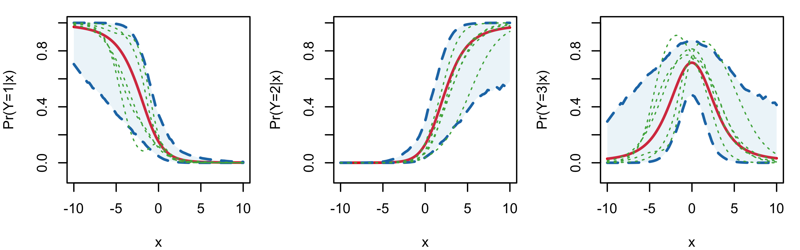
Figure 2: Illustration of the prior specification strategy (see Section 2.3 for details). In each panel, the red solid line corresponds to the prior expected probability response curve, the blue dashed lines and shaded region indicate the prior $95\%$ interval estimate, and the green dotted lines show 5 prior realizations.

2.4 Posterior inference

For Markov chain Monte Carlo (MCMC) posterior simulation, we work with a truncation approximation of the mixing distribution in the spirit of blocked Gibbs sampling for stick-breaking priors (Ishwaran and James, 2001). We favor the blocked Gibbs sampler as it results in practical model implementation and it allows for full posterior inference for general regression functionals. Hence, for posterior simulation, the mixing distribution $G_{\mathbf{x}}$ in (2) is replaced by $G_{\mathbf{x}}^{L}=$ $\sum_{\ell=1}^{L}p_{\ell}(\mathbf{x})\,\delta_{\bm{\theta}_{\ell}(\mathbf{x})}$, with $\bm{\theta}_{\ell}(\mathbf{x})$ defined as before, and $p_{\ell}(\mathbf{x})=$ $\omega_{\ell}(\mathbf{x})$, for $\ell=1,...,L-1$, whereas $p_{L}(\mathbf{x})=$ $1-\sum^{L-1}_{\ell=1}p_{\ell}(\mathbf{x})$.

The truncation level $L$ can be chosen to achieve any desired level of accuracy. For normal mixtures with LSBP weights, Rigon and Durante (2021) show that, for fixed sample size and covariates, the $L^{1}$ distance between the prior predictive distribution of the sample under $G_{\mathbf{x}}$ and $G_{\mathbf{x}}^{L}$ decreases exponentially in $L$. In practice, we can specify $L$ using the prior expectation for the partial sum of weights. Under the prior in (3), $\text{E}(\sum_{\ell=1}^{L}\omega_{\ell}(\mathbf{x}))=$ $1-\{1-\text{E}(\varphi(\mathbf{x}^{T}\bm{\gamma}))\}^{L}$, where the expectation on the right-hand-side is with respect to $\bm{\gamma}\sim N(\bm{\gamma}_{0},\Gamma_{0})$. Hence, $L$ can be selected by evaluating numerically the expectation at a few representative values in the covariate space. Note that, when $\bm{\gamma}_{0}=\mathbf{0}_{p}$, $\text{E}(\varphi(\mathbf{x}^{T}\bm{\gamma}))=0.5$, for any $\mathbf{x}$. We also recommend monitoring the posterior samples for $p_{L}(\mathbf{x})$ for different values $\mathbf{x}$ in the covariate space. Using a combination of such strategies, we worked with the (conservative) truncation level of $L=50$ for the data examples of Section 4.

Denote by $\mathbf{Y}_{i}=$ $(Y_{i1},\cdots,Y_{iC})$, with $m_{i}=$ $\sum_{j=1}^{C}Y_{ij}$, the $i$th observed response, and by $\mathbf{x}_{i}$ the corresponding covariate vector, for $i=1,\cdots,n$. We introduce a latent configuration variable $\mathcal{L}_{i}$ for each response, such that $\mathcal{L}_{i}=\ell$ if and only if $\mathbf{Y}_{i}$ is assigned to the $\ell$th mixture component. Then, the hierarchical model for the data can be expressed as

$$\begin{array}[]{rcl}\mathbf{Y}_{i}\mid\{\bm{\beta}_{j\ell}\},\mathcal{L}_{i}&\stackrel{{\scriptstyle ind.}}{{\sim}}&K(\mathbf{Y}_{i}\mid m_{i},\bm{\theta}_{\mathcal{L}_{i}})=\prod\limits_{j=1}^{C-1}Bin(Y_{ij}\mid m_{ij},\varphi(\mathbf{x}_{i}^{T}\bm{\beta}_{j\mathcal{L}_{i}})),\,\,\,i=1,\cdots,n\\ \mathcal{L}_{i}\mid\{\bm{\gamma}_{\ell}\}&\stackrel{{\scriptstyle ind.}}{{\sim}}&\sum\limits_{\ell=1}^{L}p_{i\ell}\,\delta_{\ell}(\mathcal{L}_{i}),\,\,\,i=1,\cdots,n\\ \bm{\beta}_{j\ell}\mid(\bm{\mu}_{j},\Sigma_{j})&\stackrel{{\scriptstyle ind.}}{{\sim}}&N(\bm{\mu}_{j},\Sigma_{j}),\,\,\,j=1,\cdots,C-1,\,\,\,\ell=1,\cdots,L\\ \bm{\gamma}_{\ell}&\stackrel{{\scriptstyle i.i.d.}}{{\sim}}&N(\bm{\gamma}_{0},\Gamma_{0}),\,\,\,\ell=1,\cdots,L-1\\ (\bm{\mu}_{j},\Sigma_{j})&\stackrel{{\scriptstyle ind.}}{{\sim}}&N(\bm{\mu}_{j}\mid\bm{\mu}_{0j},\Sigma_{j}/\kappa_{0j})\,IW(\Sigma_{j}\mid\nu_{0j},\Lambda_{0j}^{-1}),\,\,\,j=1,\cdots,C-1\end{array}$$ (9)

where $m_{i1}=m_{i}$, $m_{ij}=$ $m_{i}-\sum_{k=1}^{j-1}Y_{ik}$, for $j=2,\cdots,C-1$, $p_{i\ell}=$ $\varphi(\mathbf{x}_{i}^{T}\bm{\gamma}_{\ell})\prod_{h=1}^{\ell-1}(1-\varphi(\mathbf{x}_{i}^{T}\bm{\gamma}_{h}))$, for $\ell=1,\cdots,L-1$, and $p_{iL}=$ $\prod_{\ell=1}^{L-1}(1-\varphi(\mathbf{x}_{i}^{T}\bm{\gamma}_{\ell}))$.

Akin to the data $\mathbf{Y}_{i}$ and its original form $Y_{i}$, we can view the latent configuration variable $\mathcal{L}_{i}$ as the allocation of its multivariate form $\bm{\mathcal{L}}_{i}=(\mathcal{L}_{i1},\cdots,\mathcal{L}_{iL})\in\mathbb{R}^{L}$, with the connection defined as $\mathcal{L}_{i}=\ell\Longleftrightarrow\bm{\mathcal{L}}_{i}=\mathbf{1}_{\ell}$, the unit vector in $\mathbb{R}^{L}$ with the $\ell$th element equal to $1$. An important observation is that the prior model for the $\mathcal{L}_{i}$ in (9) can be equivalently defined through a continuation-ratio logits regression model for their multivariate images $\bm{\mathcal{L}}_{i}$. More specifically,

$$\bm{\mathcal{L}}_{i}\mid\{\bm{\gamma}_{\ell}\}\stackrel{{\scriptstyle ind.}}{{\sim}}Bin(\mathcal{L}_{i1}\mid 1,\eta_{1}(\mathbf{x}_{i}))\,Bin(\mathcal{L}_{i2}\mid 1-\mathcal{L}_{i1},\eta_{2}(\mathbf{x}_{i}))\cdots Bin\left(\mathcal{L}_{i,L-1}\mid 1-\sum_{k=1}^{L-2}\mathcal{L}_{ik},\eta_{L-1}(\mathbf{x}_{i})\right)$$

where $\eta_{\ell}(\mathbf{x}_{i})=$ $\varphi(\mathbf{x}_{i}^{T}\bm{\gamma}_{\ell})$, for $\ell=1,\cdots,L-1$.

The form of the hierarchical model for the data, along with the observation above, elucidate the key model property discussed in Section 2.1. Under the (truncated) LSBP prior for the covariate-dependent weights, we achieve effectively the same structure for the weights and atoms of the general mixture model. In turn, this allows us to use the Pólya-Gamma data augmentation approach (Polson et al., 2013) to update both the atoms parameters as well as the ones for the weights. In particular, for each response $\mathbf{Y}_{i}$, we introduce two sets of Pólya-Gamma latent variables, such that conditionally conjugate updates emerge for the parameters defining both the weights and the atoms. Therefore, all model parameters can be updated via Gibbs sampling. Moreover, taking advantage of the continuation-ratio logits model structure for the mixture kernel, parallel computing for the different mixing components can be adopted, facilitating implementation in applications where the number of response categories is moderate to large. Details of the posterior simulation method are presented in the Supplementary Material.

Using the posterior samples for model parameters, we can obtain full inference for any regression functional of interest. For instance, for any $j=1,\cdots,C$, posterior realizations for the marginal probability response curve, $\text{Pr}(\mathbf{Y}=j\mid G_{\mathbf{x}})$, can be computed over a grid in $\mathbf{x}$ via

$$\sum_{\ell=1}^{L}\left\{\varphi(\mathbf{x}^{T}\bm{\gamma}_{\ell}^{(t)})\prod\nolimits_{h=1}^{\ell-1}(1-\varphi(\mathbf{x}^{T}\bm{\gamma}_{h}^{(t)}))\right\}\,\left\{\varphi(\mathbf{x}^{T}\bm{\beta}_{j\ell}^{(t)})\prod\nolimits_{k=1}^{j-1}[1-\varphi(\mathbf{x}^{T}\bm{\beta}_{k\ell}^{(t)})]\right\}$$

where $\varphi(\mathbf{x}^{T}\bm{\gamma}_{L}^{(t)})=$ $\varphi(\mathbf{x}^{T}\bm{\beta}_{C\ell}^{(t)})\equiv 1$, and the superscript $(t)$ indicates the $t$th posterior sample for the model parameters.

The MCMC posterior samples can also be used to estimate the posterior predictive distribution for new response $\mathbf{Y}_{*}$ given new covariate vector $\mathbf{x}_{*}$ (and $m_{*}$). In particular, the $t$th posterior predictive sample can be obtained by first sampling the corresponding configuration variable $\mathcal{L}^{(t)}_{*}$ from the discrete distribution on $\{1,\cdots,L\}$ with probabilities $\varphi(\mathbf{x}_{*}^{T}\bm{\gamma}_{\ell}^{(t)})\prod_{h=1}^{\ell-1}(1-\varphi(\mathbf{x}_{*}^{T}\bm{\gamma}_{h}^{(t)}))$, for $\ell=1,\cdots,L$, and then sampling $\mathbf{Y}^{(t)}_{*}$ from $K(\cdot\mid m_{*},\bm{\theta}_{*}^{(t)})$, with the $j$th element of $\bm{\theta}_{*}^{(t)}$ given by $\varphi(\mathbf{x}^{T}_{*}\bm{\beta}_{j\mathcal{L}^{(t)}_{*}}^{(t)})$, for $j=1,\cdots,C-1$.

3 Specific models for ordinal regression

As discussed in Section 2.1, there is a trade-off between the flexibility of the general mixture model in (2) and the complexity of model implementation. It is thus useful to study simplified model versions, which are naturally suggested given the two building blocks of the general model. Here, we discuss the two simpler ordinal regression models that arise by retaining covariate dependence only in the atoms (Section 3.1) or only in the weights (Section 3.2). The different model versions are empirically compared in Section 4.

3.1 The common-weights model

As a first simplification, we can remove the covariate dependence from the mixture weights. That is, the ordinal regression mixture model is built from the common-weights mixing distribution $G_{\mathbf{x}}=$ $\sum_{\ell=1}^{\infty}\omega_{\ell}\,\delta_{\bm{\theta}_{\ell}(\mathbf{x})}$, such that

$$\mathbf{Y}\mid G_{\mathbf{x}}\,\sim\,\sum_{\ell=1}^{\infty}\omega_{\ell}\,K(\mathbf{Y}\mid m,\bm{\theta}_{\ell}(\mathbf{x}))$$

where the covariate-dependent atoms are defined as in the general model in (4) and (5).

Regarding the prior model for the weights, one option would be to keep the LSBP structure, that is, reduce $\mathbf{x}^{T}\bm{\gamma}_{\ell}$ in (3) to scalar parameter $\gamma_{\ell}$, with the $\gamma_{\ell}$ independent and identically normally distributed. We work instead with a prior that retains the stick-breaking formulation for the weights, but corresponds to the DP. Hence, $\omega_{1}=V_{1}$, and $\omega_{\ell}=$ $V_{\ell}\prod_{h=1}^{\ell-1}(1-V_{h})$, for $\ell\geq 2$, where $V_{\ell}\mid\alpha\stackrel{{\scriptstyle i.i.d.}}{{\sim}}\,Beta(1,\alpha)$.

Using the DP-induced prior for the weights allows connections with the well-established literature on DDP mixture models, including the early work with common-weights DDP priors, such as the ANOVA DDP (DeIorio et al., 2004), the spatial DP (Gelfand et al., 2005), and the linear DDP (DeIorio et al., 2009). In particular, the common-weights ordinal regression mixture model can be equivalently written as a DP mixture model:

$$\mathbf{Y}\mid F\,\sim\,\int K(\mathbf{Y}\mid m,(\mathbf{x}^{T}\bm{\beta}_{1},\cdots,\mathbf{x}^{T}\bm{\beta}_{C-1}))\,dF(\bm{\beta}_{1},\cdots,\bm{\beta}_{C-1})$$

where $F$ follows a DP prior with total mass parameter $\alpha$, and centering distribution defined through $\bm{\beta}_{j}\mid(\bm{\mu}_{j},\Sigma_{j})\stackrel{{\scriptstyle ind.}}{{\sim}}N(\bm{\mu}_{j},\Sigma_{j})$, for $j=1,\cdots,C-1$. The model is completed with a $Gamma(a_{\alpha},b_{\alpha})$ hyperprior for $\alpha$, and the prior for the $(\bm{\mu}_{j},\Sigma_{j})$ in (5). For prior specification, we combine the approach for the atoms in the general model with techniques for specifying the prior for the total mass DP parameter. The posterior simulation method replaces the steps for updating the weights with the update for the DP weights under blocked Gibbs sampling. The details can be found in the Supplementary Material.

With the expression for the weights appropriately adjusted, the common-weights model inherits the properties of the general model, developed in Section 2.2. The prior expectation in (8) is not affected by the form of the weights. However, the probability response curves admit a potentially less flexible form than the one in (6) under the general model. We still have a weighted combination of parametric regression functions, but now without the local adjustment afforded by covariate-dependent weights. The data analyses in Section 4 demonstrate the practical utility of the general model, but also include examples where the common-weights model yields practical, sufficiently flexible inference.

3.2 The common-atoms model

The alternative way to simplify the general model is to use mixing distribution $G_{\mathbf{x}}=$ $\sum_{\ell=1}^{\infty}\omega_{\ell}(\mathbf{x})\,\delta_{\bm{\theta}_{\ell}}$, resulting in the common-atoms mixture model:

$$\mathbf{Y}\mid G_{\mathbf{x}}\,\sim\,\sum_{\ell=1}^{\infty}\omega_{\ell}(\mathbf{x})\,K(\mathbf{Y}\mid m,\bm{\theta}_{\ell})$$

where $\bm{\theta}_{\ell}=$ $(\theta_{1\ell},\cdots,\theta_{C-1,\ell})$. The covariate-dependent weights are defined using the LSBP prior in (3). The prior model for the atoms is built from $\theta_{j\ell}\mid\mu_{j},\sigma_{j}^{2}\stackrel{{\scriptstyle ind.}}{{\sim}}N(\mu_{j},\sigma_{j}^{2})$, for $j=1,\cdots,C-1$, and $\ell\geq 1$. The model is completed with the conjugate prior for the hyperparameters: $\sigma_{j}^{2}\stackrel{{\scriptstyle ind.}}{{\sim}}IG(a_{0j},b_{0j})$, and $\mu_{j}\mid\sigma_{j}^{2}\stackrel{{\scriptstyle ind.}}{{\sim}}N(\mu_{0j},\sigma_{j}^{2}/\nu_{0j})$, for $j=1,\cdots\,C-1$, where $IG(\cdot,\cdot)$ denotes the inverse-gamma distribution.

Model implementation builds from the general model, with appropriate adjustments for the atoms. Here, $\text{E}(\text{Pr}(\mathbf{Y}=j\mid G_{\mathbf{x}}))=$ $\text{E}\left\{\varphi(\theta_{j})\prod_{k=1}^{j-1}(1-\varphi(\theta_{k}))\right\}$, for $j=1,\cdots,C$, where the expectation is taken with respect to $\theta_{j}\stackrel{{\scriptstyle ind.}}{{\sim}}N(\mu_{0j},(\nu_{0j}+1)b_{0j}/\nu_{0j}(a_{0j}-1))$ (obtained by marginalizing over the prior for $(\mu_{j},\sigma_{j}^{2})$). Hence, the prior expected marginal probability response curves are constants over the covariate space. The prior specification strategy utilizes this property, by setting $\{\mu_{0j},\nu_{0j},a_{0j},b_{0j}\}_{j=1}^{C-1}$ such that these constants correspond to prior information for the ordinal response probabilities. The key quantity is again the expectation of a logit-normal distributed random variable (discussed earlier in Section 2.3). The posterior sampling scheme is adapted from the general model, with the normal-inverse-Wishart update for the atoms parameters replaced by the univariate normal-inverse-Gamma analogue. Details are given in the Supplementary Material.

The common-atoms mixture structure offers a parsimonious model formulation, especially for problems with a moderate to large number of response categories. On the other hand, the simplified model form involves a potential limitation. The marginal and conditional probability response curves have the form in (6) and (7), respectively, with $\theta_{j\ell}(\mathbf{x})$ replaced by $\theta_{j\ell}$. Hence, the covariates inform the shape of the regression curves only through the mixture weights. As a practical consequence, the common-atoms model typically activates a larger number of effective mixture components to estimate the regression relationship, and it thus encounters a higher risk of overfitting for problems with a moderate to large number of covariates. This point is illustrated with the data examples of Section 4.

4 Data illustrations

4.1 Synthetic data examples

We present two simulation examples to demonstrate the proposed modeling framework, including comparative study of the common-weights model, the common-atoms model, and the general model. To facilitate graphical illustrations, we consider a single (continuous) covariate and an ordinal response with $C=3$ categories. In both examples, $n$ pairs of ordinal response and covariate $(\mathbf{Y}_{i},x_{i})$ are generated, where $x_{i}\stackrel{{\scriptstyle i.i.d.}}{{\sim}}Unif(-10,10)$, such that with the intercept, the covariate vector is $\mathbf{x}_{i}=(1,x_{i})^{T}$. The posterior analyses are based on 4000 posterior samples collected every 5 iterations from a Markov chain of 30000 iterations, with the first 10000 samples being discarded.

First experiment

We generate $n=100$ responses from a probit model, that is, we first sample normally distributed latent continuous variables $\tilde{y}_{i}$, and then discretize the $\tilde{y}_{i}$ with cut-off points to get the ordinal responses $\mathbf{Y}_{i}$, for $i=1,\cdots,n$. The objective is to study how the different models handle the challenge of recovering standard regression relationships for which the nonparametric mixture model structure is not necessary.

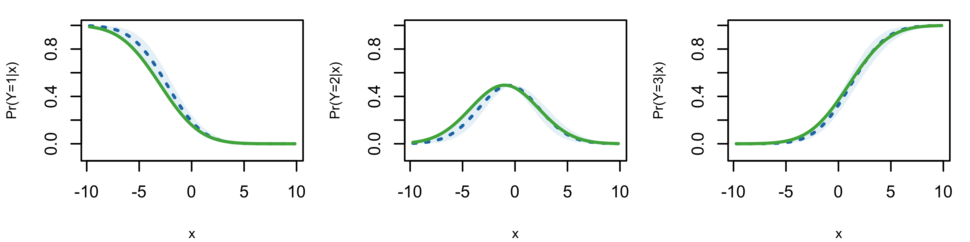
(a) Probit model.

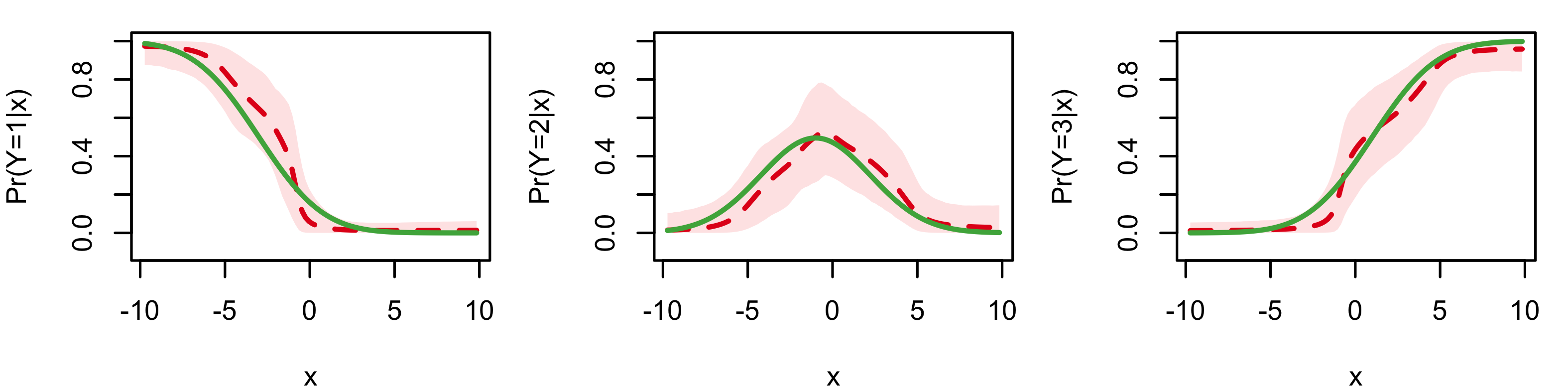
(b) Common-weights model.

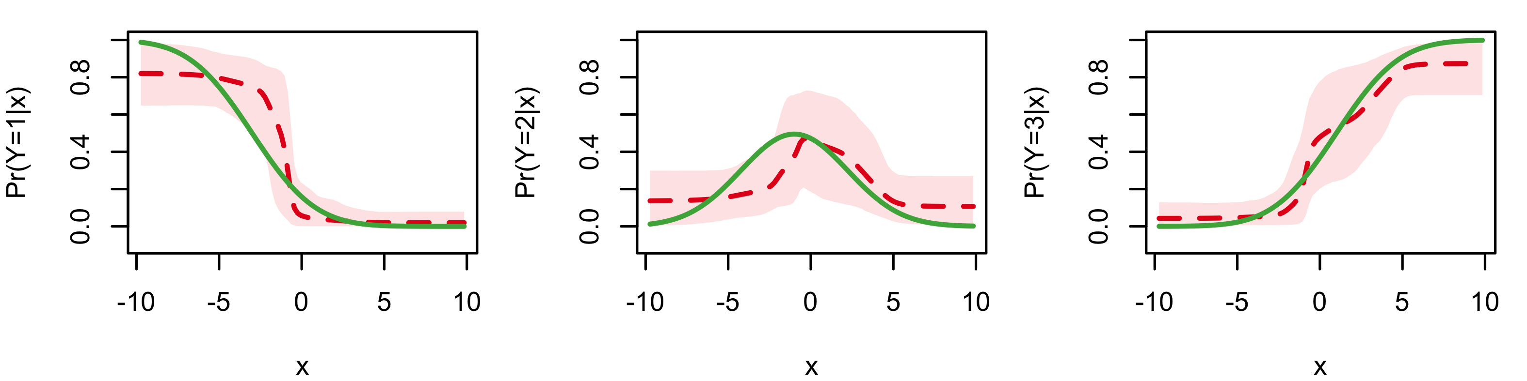
(c) Common-atoms model.

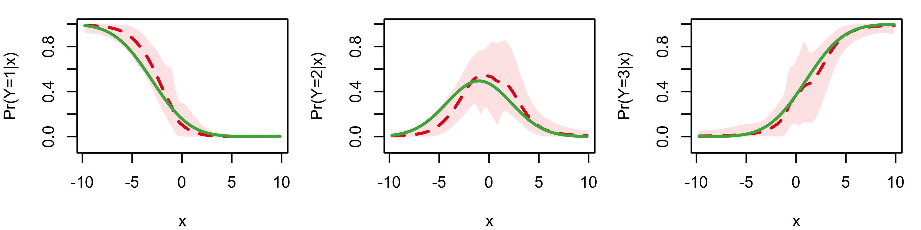
(d) General model.

Figure 3: First simulation example. Inference results for the marginal probability response curves, under the baseline prior for the nonparametric models. In each panel, the dashed line and shaded region correspond to the posterior mean and $95\%$ credible interval estimates, whereas the (green) solid line denotes the true regression function.

The nonparametric mixture models are applied to the data, using the (non-informative) baseline prior for their hyperparameters. Figure 3 plots posterior point and interval estimates for the marginal probability response curves, including, as a reference point, estimates under the parametric probit model used to generate the data. As expected, the nonparametric models result in wider posterior uncertainty bands than the parametric model. In terms of recovering the underlying regression curves, the common-atoms model is less effective than the common-weights and the general model. As discussed in Section 3.2, this can be explained from the common-atoms model property that the regression curve shapes are adjusted essentially only through the mixture weights. The findings from the graphical comparison are supported by results from formal comparison, using the posterior predictive loss criterion from Gelfand and Ghosh (1998) (see the Supplementary Material). The model comparison criterion suggests comparable performance for the common-weights and general models, whereas both outperform the common-atoms model.

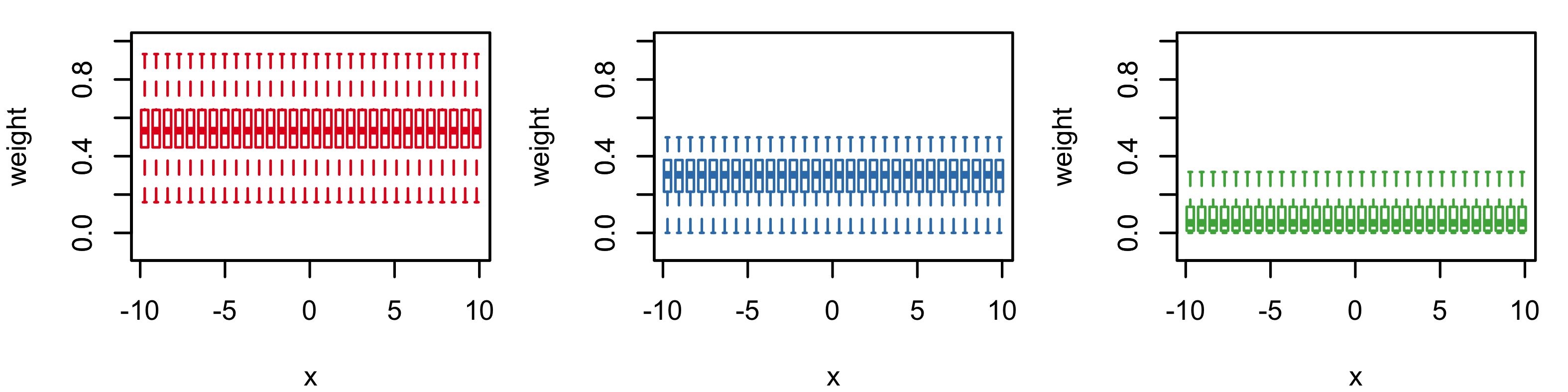
(a) Common-weights model.

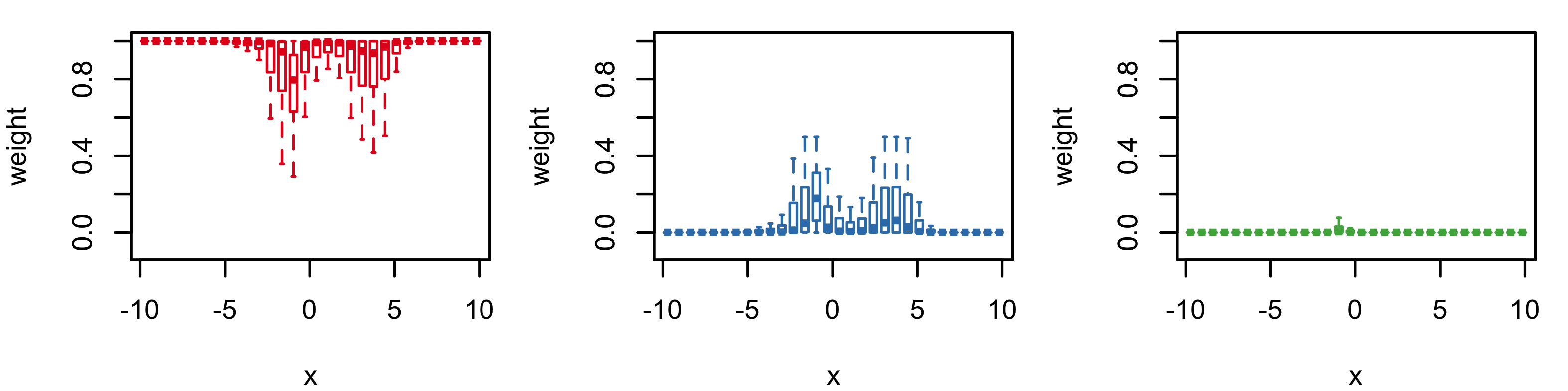
(b) Common-atoms model.

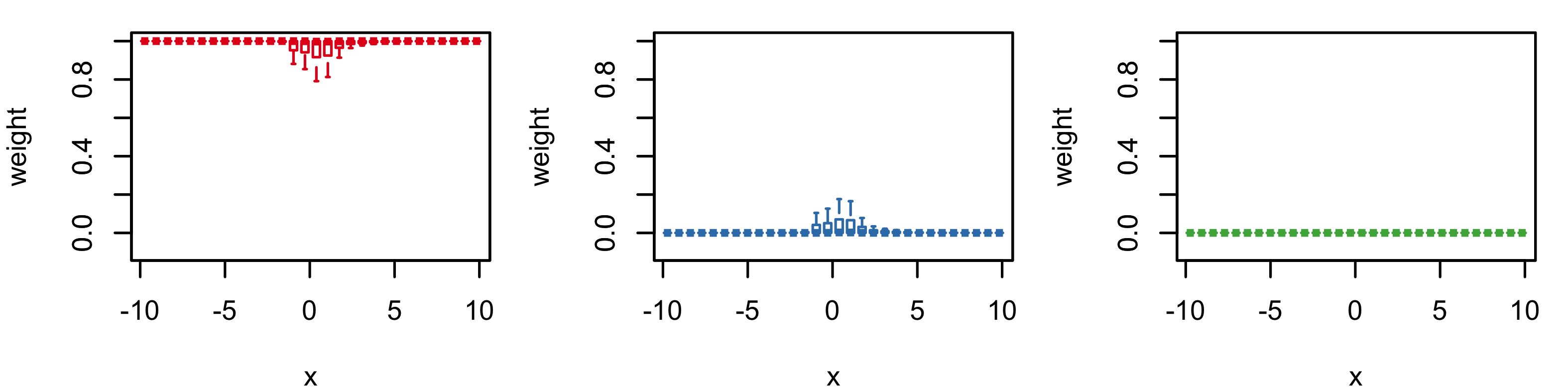
(c) General model.

Figure 4: First simulation example. Box plots of the posterior samples for the three largest mixture weights under each of the nonparametric models.

To further explore how the different nonparametric models utilize the mixture structure, Figure 4 shows the posterior distributions of the three largest mixture weights across covariate values. (A plot that contains the posterior mean estimates for the weights and the corresponding atoms is given in the Supplementary Material.) The general model is the most efficient in terms of the number of effective mixture components, using a second component (with small weight) only for covariates values around $0$. This is to be expected, since it is those covariate values that result in practically relevant differences between the probit regression function (used to generate the data) and the logistic regression kernel. The common-atoms model activates effectively one extra component for covariate values where the regression functions are not flat. Compared to the general model, it places larger weights on the second component to account for the constant atoms. On the other hand, the mixture weights can not change with the covariates for the common-weights model. Hence, in order to recover the probit regression function, this model utilizes effectively three mixture components, with the second and third assigned larger (global) weight than the other two models.

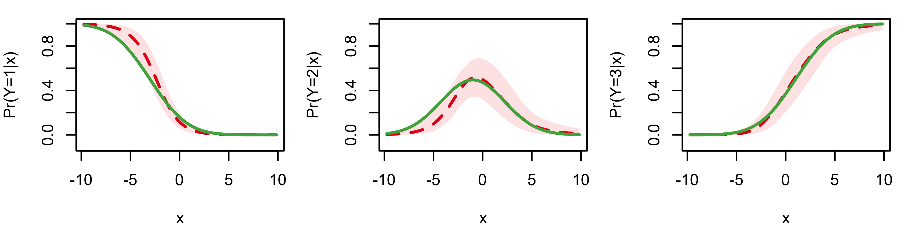
(a) Common-weights model.

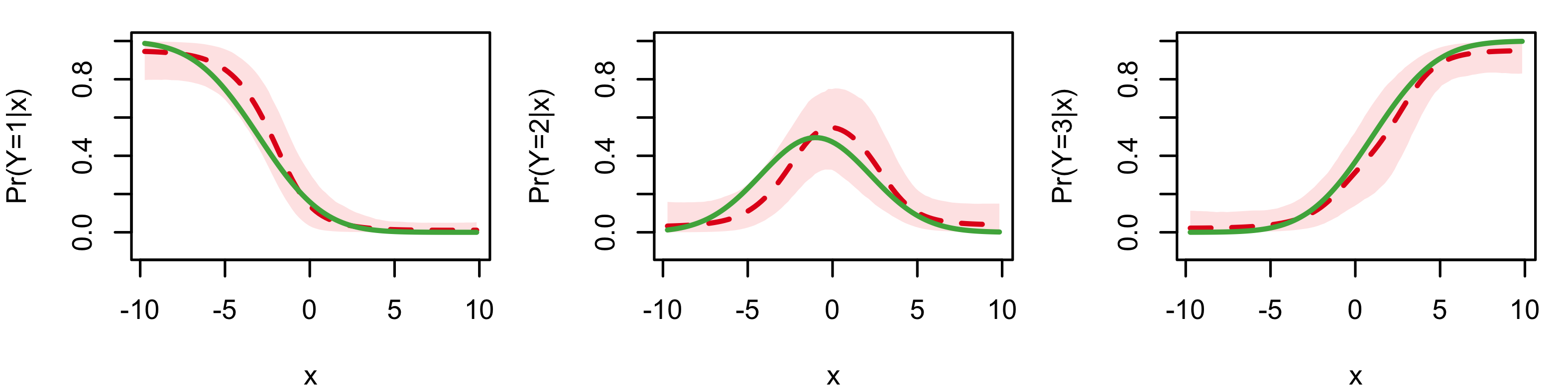
(b) Common-atoms model.

(c) General model.

Figure 5: First simulation example. Inference results for the marginal probability response curves, under the informative prior specification. In each panel, the dashed line and shaded region correspond to the posterior mean and $95\%$ credible interval estimates, whereas the (green) solid line denotes the true regression function.

The sample size for this example was intentionally taken to be relatively small, in order to study sensitivity to the prior choice, as well as to demonstrate the practical utility of a more focused prior specification approach. If the monotonicity of two of the regression functions was in fact available as prior information, such information can be incorporated into the model, as discussed in Section 2.3. Indeed, Figure 5 reports posterior inference results under a more informative prior specification, the details of which can be found in the Supplementary Material. Comparing with Figure 3, we notice more accurate posterior mean estimates and a reduction in the width of the posterior uncertainty bands, the improvement being particularly noteworthy for the common-atoms model.

Second experiment

Here, our objective is to highlight the benefits of local, covariate-dependent weights in capturing non-standard shapes of probability response curves. To this end, we generate the responses from a three component mixture of multinomial distributions, expressed in their continuation-ratio logis form. That is, $\mathbf{Y}\sim$ $\sum_{k=1}^{3}w_{k}(\mathbf{x})\,K(\mathbf{Y}\mid m,\bm{\theta}_{k}(\mathbf{x}))$, where $\theta_{jk}(\mathbf{x})=$ $b_{jk0}+b_{jk1}x$, for $j=1,2$ and $k=1,2,3$. To introduce covariate dependence also in the weights, we compute $p_{j\mathbf{x}}=$ $\Phi(a_{j0}+a_{j1}x)$, for $j=1,2$, where $\Phi$ is the standard normal distribution function, and set $(w_{1}(\mathbf{x}),w_{2}(\mathbf{x}),w_{3}(\mathbf{x}))=$ $(p_{1\mathbf{x}},(1-p_{1\mathbf{x}})p_{2\mathbf{x}},(1-p_{1\mathbf{x}})(1-p_{2\mathbf{x}}))$. The parameters for the weights and atoms are chosen such that the resulting probability response curves have non-standard shapes (see Figure 6). We perform the experiment with two sample sizes, $n=200$ and $n=800$.

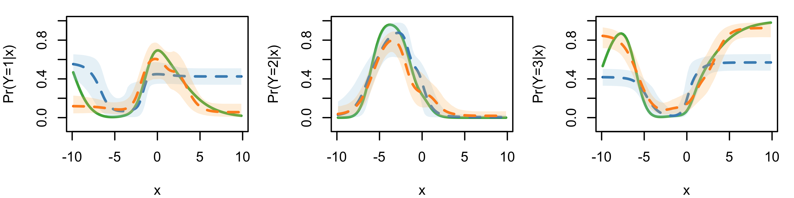
(a) Common-weights and common-atoms models ($n=200$).

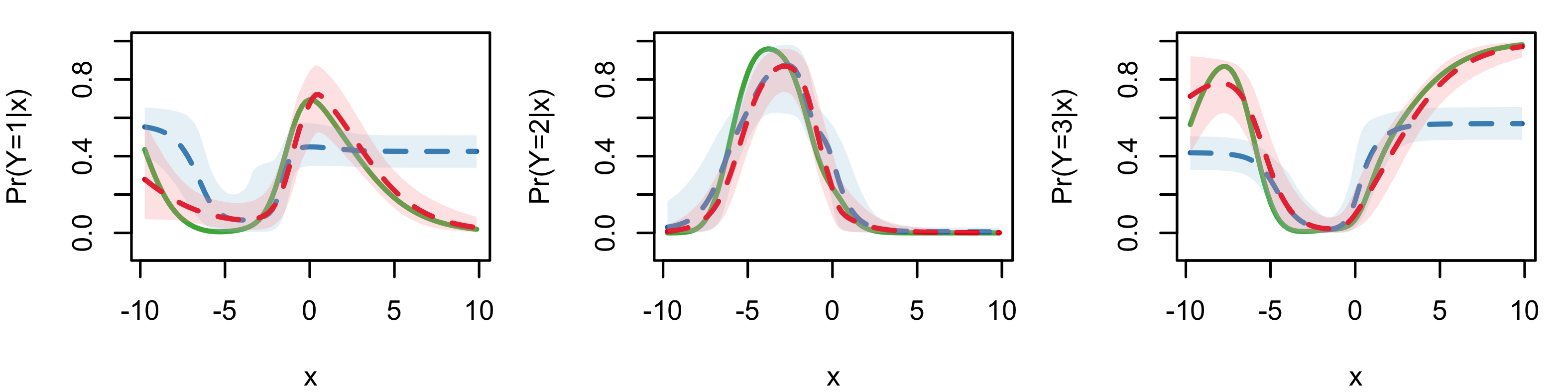
(b) Common-weights and general models ($n=200$).

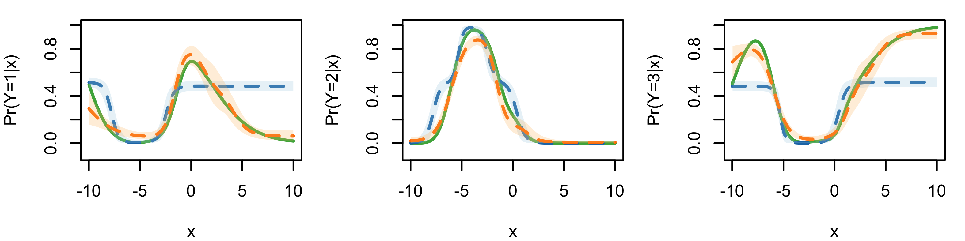
(c) Common-weights and common-atoms models ($n=800$).

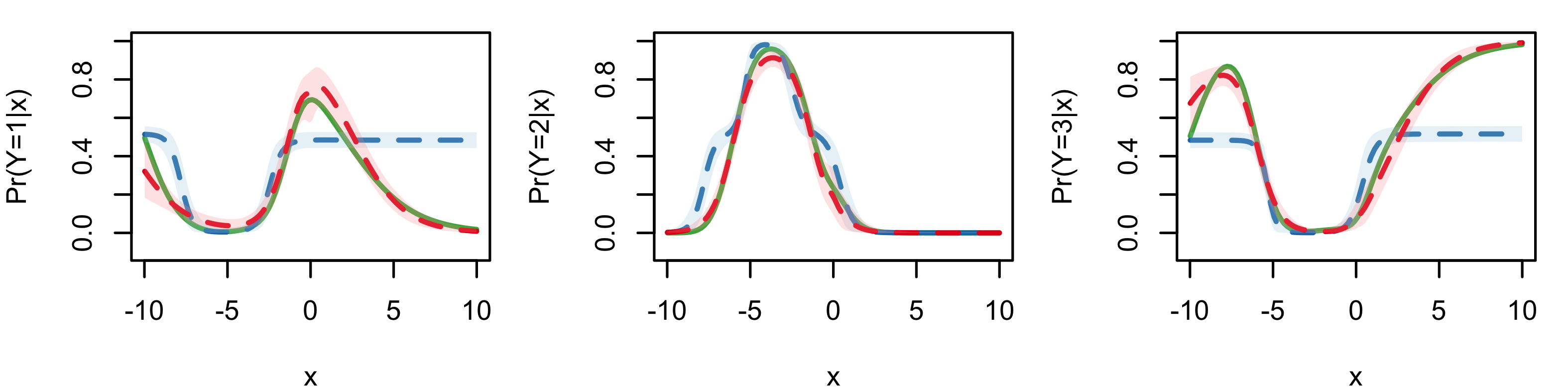
(d) Common-weights and general models ($n=800$).

Figure 6: Second simulation example. Posterior mean and $95\%$ credible interval estimates for the marginal probability response curves under the common-weights (blue line and shaded region), common-atoms (orange line and shaded region), and general (red line and shaded region) models. In each panel, the green solid line is the true regression function.

The prior hyperparameters for the atoms are set according to the baseline choice. For the common-atoms and general models, we specify the LSBP prior hyperparameters $(\bm{\gamma}_{0},\Gamma_{0})$ to favor a priori more mixture components in the interval of covariate values $(-10,0)$ where there is more variation in the regression functions. We note however that the prior specification is still fairly non-informative regarding the shape of the regression functions. In particular, under all three models, the prior mean estimates for the probability response curves are flat, and the prior $95\%$ interval estimates span a substantial portion of the unit interval (the prior estimates are shown in the Supplementary Material).

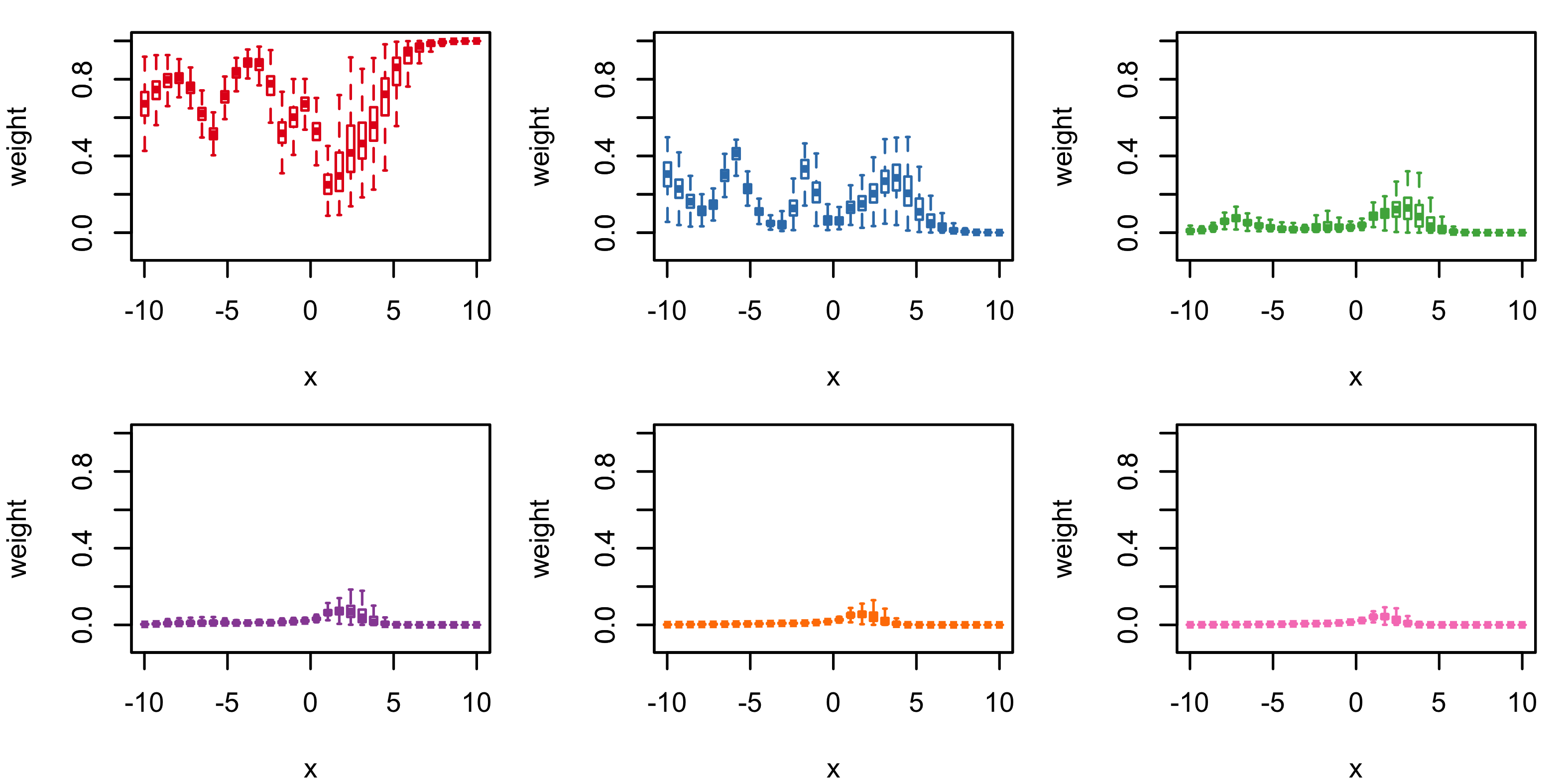
(a) Common-atoms model.

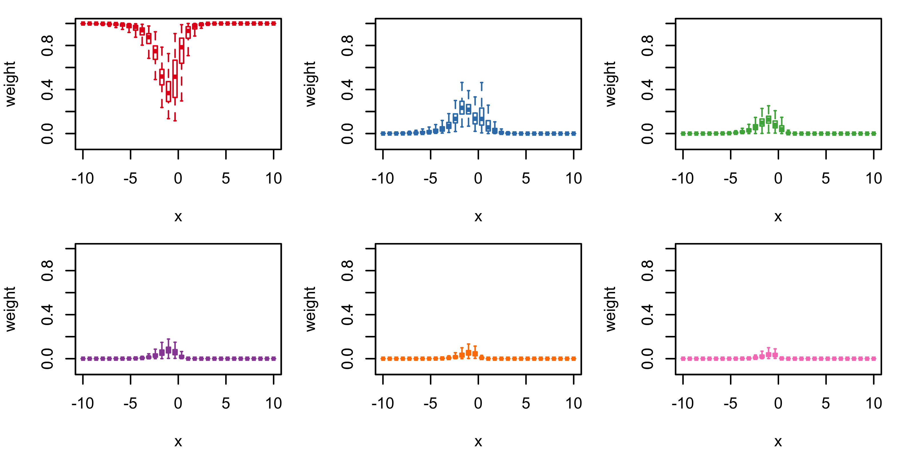
(b) General model.

Figure 7: Second simulation example. Box plots of the posterior samples for the six largest mixture weights, under the common-atoms and general models.

Inference results under the general and common-atoms models are contrasted with the common-weights model in Figure 6. As expected, the common-weights model does not recover well the non-standard regression functions for the first and third response categories. The two models that use covariate-dependent mixture weights perform notably better, with the general model resulting overall in more accurate estimation. This ranking in model performance is also supported by the posterior predictive loss criterion (refer to the Supplementary Material for details). Increasing the sample size results in more precise point estimates and more narrow posterior uncertainty bands.

Focusing on the models with covariate-dependent mixture weights (and the data set with $n=800$), Figure 7 explores the posterior distribution of the six largest weights over the covariate space. For both models, it is essentially the first three largest weights that, given the data, define the probability vector of weights. However, we note the more local adjustment in the two largest weights under the common-atoms model, which becomes more pronounced in parts of the covariate space where the probability curves change more drastically. This is compatible with the common-atoms model’s structure that seeks to fit the regression functions with atoms that do not change across the covariate space.

4.2 Credit ratings of U.S. firms

We consider data on Standard and Poor’s (S$\&$P) credit ratings for 921 U.S. firms in 2005 (Verbeek, 2008). The ordinal response is the firm’s credit rating, originally recorded on a scale with seven categories. Since there were only 17 firms with rating of 1 or 7, and to facilitate illustration of inference results, we combine the responses in the first two and last two categories. We thus obtain an ordinal response scale ranging from 1 to 5, with higher ratings indicating higher creditworthiness. The data set includes five company characteristics that serve as covariates: book leverage (ratio of debt to assets), $x_{1}$; earnings before interest and taxes divided by total assets, $x_{2}$; standardized log-sales (proxy for firm size), $x_{3}$; retained earnings divided by total assets (proxy for historical profitability), $x_{4}$; and working capital divided by total assets (proxy for short-term liquidity), $x_{5}$.

The three nonparametric models were applied to the data, using the baseline choice for the atoms prior hyperparameters, and priors for the weights hyperparameters that favor a moderate to large number of distinct mixture components $n^{*}$ (i.e., number of distinct $\mathcal{L}_{i}$ in the notation of Section 2.4). Given the number of covariates, one would expect that the common-atoms model requires larger $n^{*}$ compared to the models with covariate-dependent atoms. Indeed, the posterior median for $n^{*}$ is $8$, $12$, and $21$ under the common-weights, general, and common-atoms model, respectively; in fact, the common-atoms model did not produce a posterior draw for $n^{*}$ smaller than $10$. The relative inefficiency of the common-atoms model is also reflected in its larger penalty term for the posterior predictive loss criterion. The model comparison criterion essentially does not distinguish between the general and common-weights models, and inference results are overall similar under these two models. More details from the model comparison are included in the Supplementary Material. Here, we discuss results under the common-weights model.

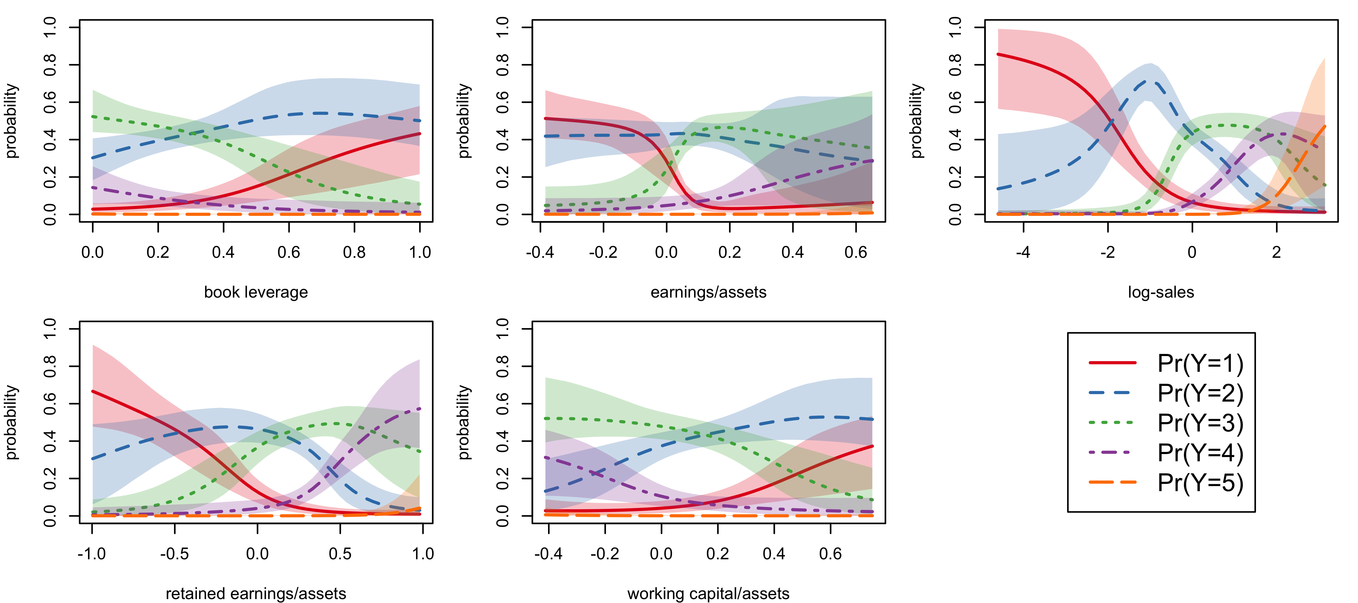
Figure 8: Credit ratings data. Posterior mean (lines) and $95\%$ interval (shaded regions) estimates of probability response curves $\pi_{j}(x_{s})$. Estimates for all five response categories are displayed in a single panel for each covariate.

We estimate first-order effects for each covariate $x_{s}$ (denoted by $\pi_{j}(x_{s})$, for $j=1,\cdots,5$), by computing posterior realizations for $\text{Pr}(\mathbf{Y}=j\mid G_{\mathbf{x}})$ in (6) at a grid over the observed range for $x_{s}$, keeping the values of the other covariates fixed at their observed average. The resulting point and interval estimates are displayed in Figure 8. The estimates reveal some interesting relationships between the firm’s characteristics and its credit rating. For instance, debt may help to fuel growth of the firm, while uncontrolled debt levels can lead to credit downgrades. Hence, an important question pertains to the relevant debt to assets ratio. The substantial increase in the probability of the lowest credit rating when book leverage gets larger than 0.4 (top left panel of Figure 8) suggests that the desirable ratio may not exceed $0.4$. Moreover, there is a positive association between standardized log-sales (a proxy for firm size) and the firm’s credit rating. The probability of the lowest credit rating decreases at a particular rate for low to moderate log-sales values, with the probability becoming exceedingly small for larger firms. The probabilities for ratings 2, 3 and 4 peak at increasingly larger log-sales values, and the probability of the highest rating is practically zero for low to moderate log-sales values and is increasing for the largest firms.

Similarly to the first-order effects estimates, we can obtain inference for second-order probability response surfaces for any pair of covariates $(x_{s},x_{s^{\prime}})$, denoted by $\pi_{j}(x_{s},x_{s^{\prime}})$, for $j=1,\cdots,5$. As an illustration of the model’s capacity to accommodate interaction effects among the covariates, Figure 9 plots posterior mean estimates for the second-order effects corresponding to earnings divided by total assets ($x_{2}$) and standardized log-sales ($x_{3}$).

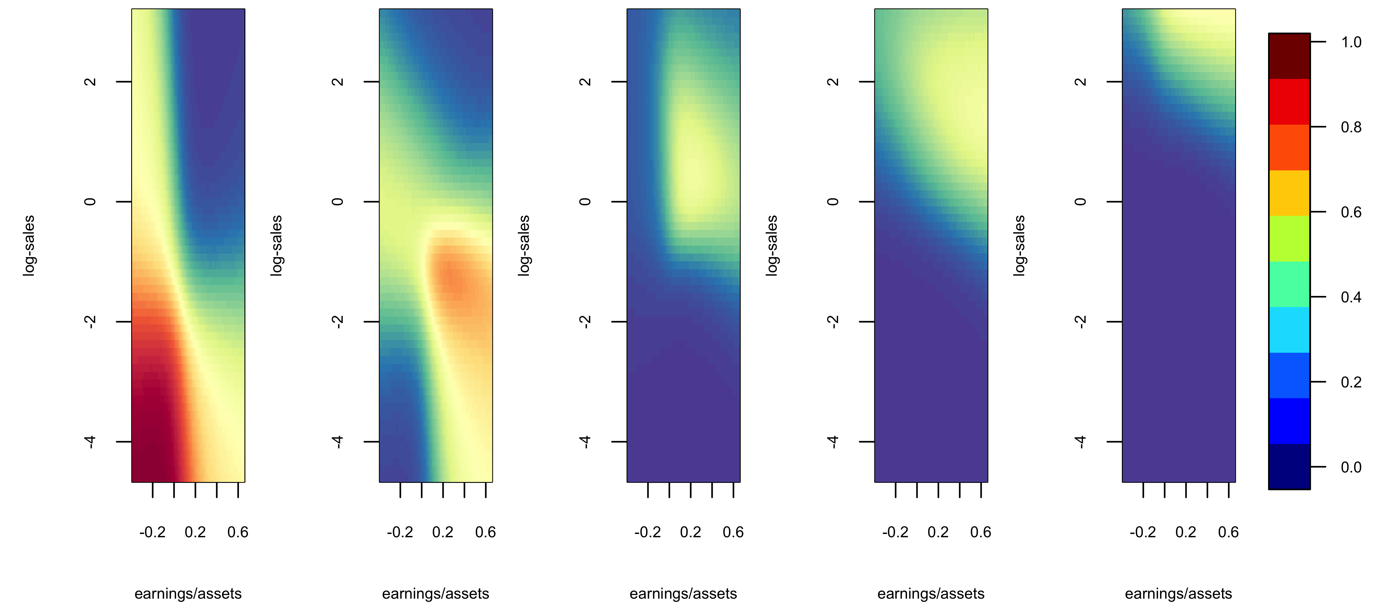
Figure 9: Credit ratings data. Posterior mean estimates of probability response surfaces $\pi_{j}(x_{2},x_{3})$, for $j=1,\cdots,5$ (from left to right).

The Supplementary Material includes additional results from this data analysis. In particular, the nonparametric modeling approach is shown to outperform the parametric continuation-ratio logits regression model. Moreover, we study the nonparametric model’s performance in prediction, studying how the posterior probability of obtaining investment grade (rating of 3 or higher) changes when each of the covariates changes its value from the 25th to the 75th observed percentile.

4.3 Developmental toxicology data example

Segment II developmental toxicity studies provide an important area of application under the extended problem setting. In these studies, at each experimental toxin level, $x_{i}$, a number, $n_{i}$, of pregnant laboratory animals (dams) are exposed to the toxin and the total number of implants, $m_{id}$, the number of non-viable fetuses (undeveloped embryos and/or prenatal deaths), $R_{id}$, and the number of live malformed pups, $y_{id}$, from each dam are recorded. Thus, the data structure, $\{(x_{i};R_{id},y_{id},m_{id}-R_{id}-y_{id}):i=1,\cdots,N;d=1,\cdots,n_{i}\}$, falls in the extended ordinal regression setting, indeed, with replicated responses at each value of the single covariate (toxin level).

We consider data from a study where diethylene glycol dimethyl ether (DYME), an organic solvent, is evaluated for toxic effects in pregnant mice (Price et al., 1987). The data is available from the National Toxicology Program database. The study involves four active toxin levels at 0.0625, 0.125, 0.25 and 0.5 g/kg and a control group, with a number of dams (ranging from 18 to 24) assigned to each group. The empirical proportions of embryolethality, malformation, and combined negative outcomes (plotted in Figure 10) suggest an increasing trend across toxin levels, although with no obvious parametric form for each dose-response curve. Due to the inherent heterogeneity of both the dams and the pups’ reaction to the toxin, the variation in outcomes is vast.

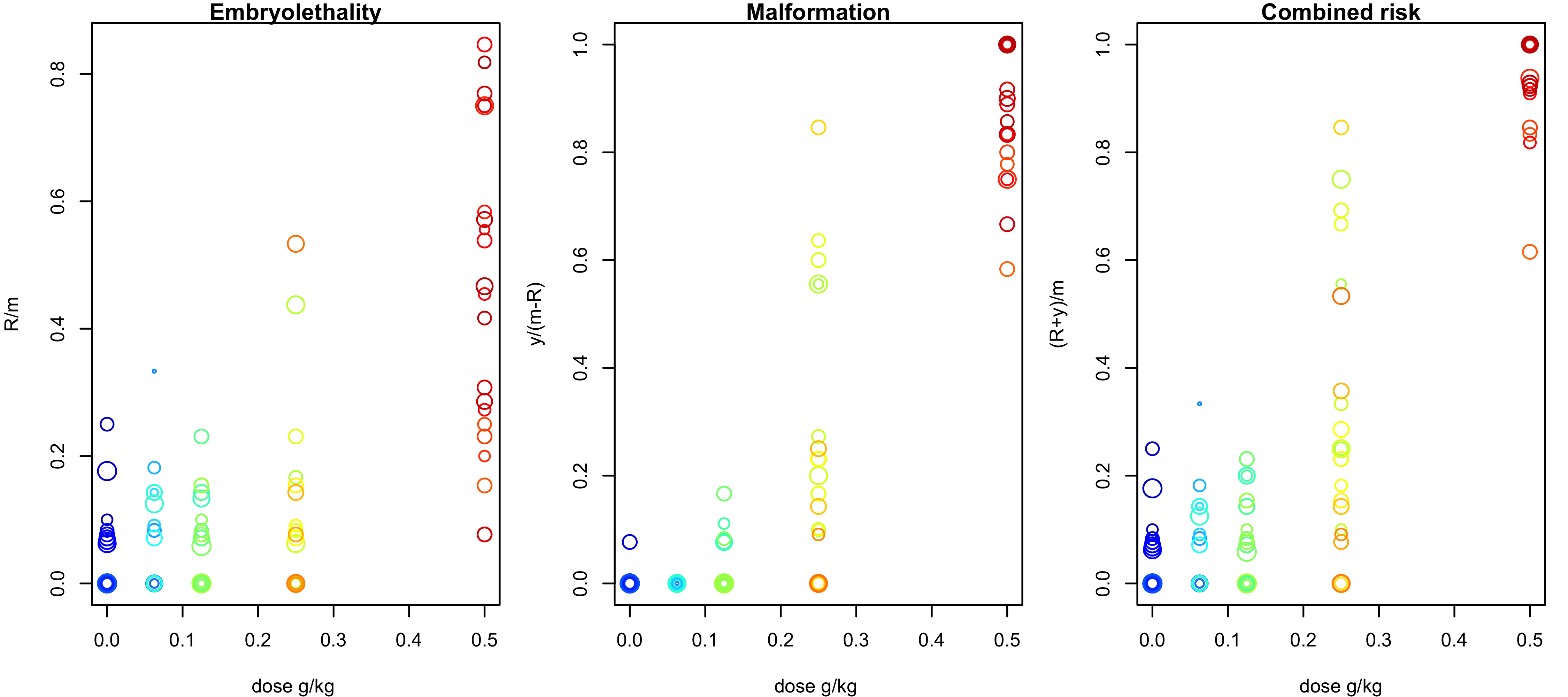
Figure 10: DYME data. In each panel, a circle corresponds to a particular dam and the size of the circle is proportional to the number of implants. The coordinates of the circle are given by the toxin level and the proportion of the specific endpoint: non-viable fetuses among implants (left panel); malformations among live pups (middle panel); combined negative outcomes among implants (right panel).

Because in Segment II toxicity experiments exposure occurs after implantation, we assume a distribution for the number of implants, $m$, that does not depend on the toxin level. In particular, we work with a shifted Poisson distribution, $f(m\mid\lambda)=$ $e^{-\lambda}\lambda^{m-1}/(m-1)!$, for $m\geq 1$. Hence, the modeling focus is on the toxin-dependent conditional distribution for the number of non-viable fetuses and malformations, $(R,y)$, given $m$, for which we explore the proposed nonparametric mixture models.

The main objective of developmental toxicity studies is to examine the relationship between the toxin level and the probability of the various responses. We focus on the endpoints of embryolethality, fetal malformation, and combined negative outcomes. The respective dose-response curves are defined by the toxin-dependent probability of a non-viable fetus, conditional probability of malformation for a live pup, and probability of either of the two negative outcomes. To develop the expressions for the dose-response curves, it is helpful to consider the underlying standard ordinal responses. In particular, we denote by $\tilde{R}$ and $\tilde{y}$ the non-viable fetus indicator and the malformation indicator for a live pup, respectively. Therefore, for a generic dam with $m$ implants exposed to toxin level $x$, $\{\tilde{R}_{q}:q=1,\cdots,m\}$ are the non-viable fetus indicators, and $\{\tilde{y}_{l}:l=1,\cdots,m-\sum_{q=1}^{m}\tilde{R}_{q}\}$ the malformation indicators for the live pups, such that the (extended) ordinal response is $(R,y,m-R-y)$, where $R=\sum_{q=1}^{m}\tilde{R}_{q}$ and $y=\sum_{l=1}^{m-R}\tilde{y}_{l}$. Based on (6) and (7), the implied expressions for the dose-response curves of embryolethality, $D(x)=$ $\text{Pr}(\tilde{R}=1\mid G_{\mathbf{x}})$, malformation, $M(x)=$ $\text{Pr}(\tilde{y}=1\mid\tilde{R}=0,G_{\mathbf{x}})$, and combined risk, $r(x)=$ $\text{Pr}(\tilde{R}=1\,\,\text{or}\,\,\tilde{y}=1\mid G_{\mathbf{x}})=$ $\text{Pr}(\tilde{R}=0\,\,\text{and}\,\,\tilde{y}=1\mid G_{\mathbf{x}})$ + $\text{Pr}(\tilde{R}=1\mid G_{\mathbf{x}})$, are given by

$$\begin{split}&D(x)\,=\,\sum_{\ell=1}^{\infty}\omega_{\ell}(\mathbf{x})\,\varphi(\mathbf{x}^{T}\bm{\beta}_{1\ell});\quad M(x)\,=\,\sum_{\ell=1}^{\infty}\frac{\omega_{\ell}(\mathbf{x})[1-\varphi(\mathbf{x}^{T}\bm{\beta}_{1\ell})]}{\sum_{\ell=1}^{\infty}\omega_{\ell}(\mathbf{x})[1-\varphi(\mathbf{x}^{T}\bm{\beta}_{1\ell})]}\,\varphi(\mathbf{x}^{T}\bm{\beta}_{2\ell});\\ &r(x)\,=\,1-\sum_{\ell=1}^{\infty}\omega_{\ell}(\mathbf{x})\,[1-\varphi(\mathbf{x}^{T}\bm{\beta}_{1\ell})][1-\varphi(\mathbf{x}^{T}\bm{\beta}_{2\ell})],\end{split}$$

with $\mathbf{x}=(1,x)^{T}$, and the weights $\omega_{\ell}(\mathbf{x})$ defined in (3).

A practically relevant modeling aspect revolves around possible monotonicity restrictions for the dose-response functions. Developmental toxicity studies involve a small number of administered toxin levels. Hence, under nonparametric mixture models for the categorical responses, a monotonic trend in the prior expectation for the dose-response curves is needed for effective interpolation and extrapolation inference. This is discussed in Kottas and Fronczyk (2013) and Fronczyk and Kottas (2014) under common-weights DDP mixture models, and is also relevant in our model setting. Therefore, this is an application area for which the common-atoms model is not a practical option, and, indeed, we explore only the common-weights and the general model. Using for these two models the prior specification strategy of Section 2.3, we can incorporate a non-decreasing trend in the prior expected dose-response curves (prior point and interval estimates are displayed in the Supplementary Material). We note however that prior (and thus posterior) realizations for the dose-response curves are not structurally restricted to be non-decreasing.

The general model outperforms the common-weights model based on the posterior predictive loss criterion. We also perform model checking (for the general model), using cross-validated posterior predictive samples, which shows no evidence of lack of fit. Here, we present results under the general model, although inferences are similar under the common-weights model. Details on model assessment and comparison, and inference results under the common-weights model are included in the Supplementary Material.

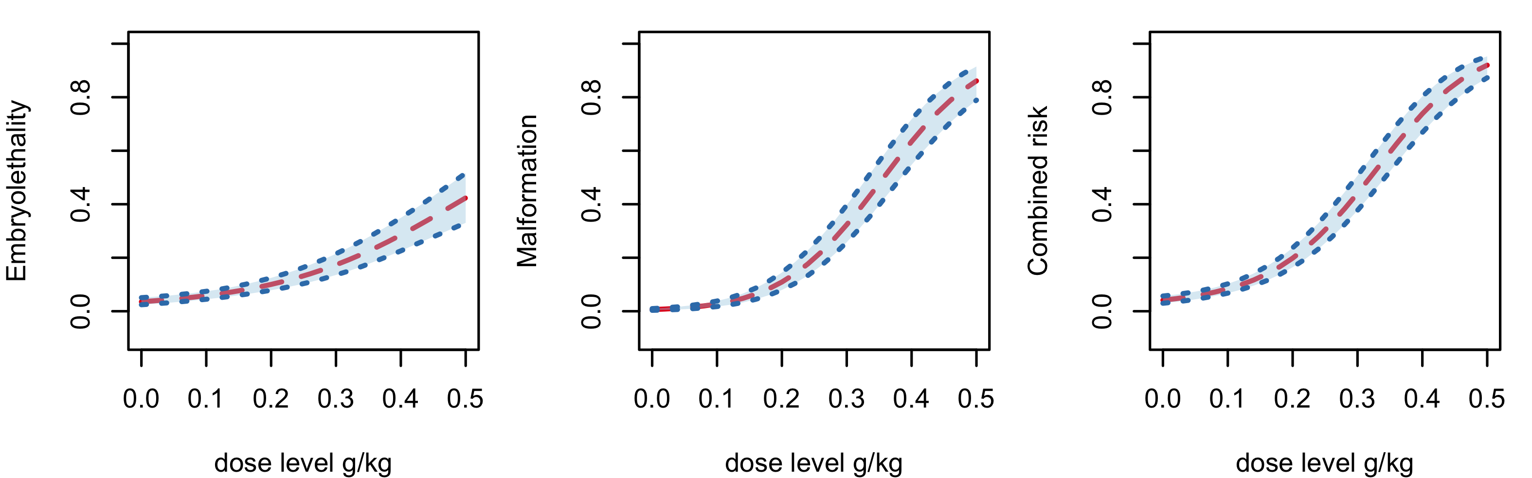
Figure 11: DYME data. Under the general model, posterior mean (red dashed line) and 95% interval estimates (blue dotted line and shaded region) for the dose-response curves.

Figure 11 plots the posterior mean and 95$\%$ uncertainty bands for the dose-response curves. The embryolethality dose-response function depicts a slowly increasing trend. The conditional probability of malformation has a skewed shape, with larger uncertainty between the last two observed toxin levels. The combined risk function is similar in shape to the malformation dose-response curve, though shifted up slightly and with decreased uncertainty bands. Regarding inference for the response distributions corresponding to the two endpoints, estimates for the probability mass functions for the number of non-viable fetuses given a specific number of implants are presented in the Supplementary Material. Figure 12 displays estimates for the conditional probability mass functions of the number of malformations given a specified number of implants and the associated number of non-viable fetuses. The model uncovers non-standard distributional shapes, such as the ones at toxin levels $x=0.25$ g/kg and $x=0.5$ g/kg. Also noteworthy is the smooth evolution from right to left skewness in the probability mass functions as the toxin level increases.

Figure 12: DYME data. Under the general model, posterior mean (“o”) and 95$\%$ uncertainty bands (dotted lines) for the conditional probability mass function for the number of malformations given $12$ implants and $2$ non-viable fetuses, $f(y\mid m=12,R=2,G_{\mathbf{x}})$, for the five observed toxin levels and for the new value of $x=0.375$ g/kg.

5 Discussion

Seeking to incorporate flexibility in both the response distribution and the ordinal regression relationship, we have developed a Bayesian nonparametric mixture modeling framework for ordinal regression. We approach the ordinal regression problem by directly modeling the discrete response distribution. The similarity between the logit stick-breaking prior and the continuation-ratio logits structure provides an elegant way of incorporating covariate effects in both the weights and the atoms of the mixture model, leading to the general model. To investigate the trade-off between model flexibility and implementation complexity, we introduce two simpler models that arise by retaining covariate dependence only in the atoms (common-weights model) or only in the weights (common-atoms model). The proposed models form a comprehensive toolbox that spans a wide range of flexibility in modeling ordinal regression relationships. Viewing the two simpler models as the building blocks of the general model enables us to explore model properties and develop inference algorithms under a unified framework. The practical advantage of the proposed models lies in the convenience in prior specification and the computational efficiency of the posterior simulation method. With regard to the latter, the key feature is the combination of the continuation-ratio logits representation for the mixture kernel with the Pólya-Gamma data augmentation technique.

A practical consideration is which model to apply to a specific problem. The principal rule is to exploit model flexibility while accounting for restrictions induced by available information. Regarding the latter, the developmental toxicology data analysis (Section 4.3) provides an example where one of the simpler models can be eliminated from consideration based on knowledge about the problem under study. As for model flexibility, the other data examples of Section 4 were chosen to study different scenarios for suitability of the simplified models, as they pertain to the complexity of the probability response curves, the sample size, and the number of covariates. The common-weights model can not take advantage of the local adjustment offered by covariate-dependent weights, and this may be an issue for non-standard ordinal regression relationships. Among the two simpler model specifications, the common-atoms model is a more suitable choice when expecting complicated covariate-response relationships. The caveat is that this model activates a large number of effective mixture components, thus increasing the computational cost and facing the potential risk of overfitting. Inheriting features from both of its building blocks, the general model offers the most versatile structure. Its benefits emerge especially in applications with sufficiently large amounts of data and non-standard regression relationships, as demonstrated by the second synthetic data example of Section 4.1. Nonetheless, in applications with small to moderate sample sizes and moderate to large number of response categories, the two simpler models are useful options to consider.

The scalability of the proposed models is built upon the continuation-ratio logits structure, which boosts computation in two ways. First, it implies a conditional independence structure for category-specific parameters, allowing partial parallel computing across response categories. In addition, the MCMC algorithm can be potentially replaced by a mean-field variational inference approach (e.g., Blei and Jordan, 2006). Taking advantage of the Pólya-Gamma technique, the variational strategy for our models can be framed within the well-established exponential family setting, for which there exists a closed-form coordinate ascent variational inference algorithm (Blei et al., 2017). Therefore, there is exciting potential to scale up the models to handle ordinal regression problems with large amounts of data, as in, e.g., business and marketing applications.

The ordinal regression problem we have explored in this work forms a key building block for more general model settings involving ordinal responses. A primary feature of the proposed modeling framework is its modularity. As a specific example, the model structure can be embedded in a hierarchical framework to develop general, nonparametric inference for longitudinal ordinal regression. Repeated measurements of ordinal responses are typically measured with covariates over time. A possible way to approach such problems could be built upon models that allow the ordinal regression relationships at each particular time point to be estimated in a flexible fashion, combined with a hyper-model for evolving temporal dynamics. We will report on this modeling extension in a future manuscript.

Supplementary material

The Supplementary Material includes details for the MCMC algorithms (Section S1) and the prior specification strategy (Section S2), and additional results for the data examples (Section S3).

Supplementary Material: Structured Mixture of Continuation-ratio Logits Models for Ordinal Regression

S1 MCMC posterior simulation details

The general model

The development of the posterior simulation method for the general model (9) relies heavily on effectively the same structure for the weights and atoms of the mixture model. The Pólya-Gamma data augmentation approach are used to update parameters defining both the weights and atoms, leading to conditionally conjugate update for all parameters. Denote the Pólya-Gamma distribution with shape parameter $b$ and tilting parameter $c$ by $PG(b,c)$. Specifically, for each $\mathbf{Y}_{i}$, we introduce two groups of Pólya-Gamma latent variables $\bm{\xi}_{i}=(\xi_{i1},\cdots,\xi_{i,L-1})$ and $\bm{\zeta}_{i}=(\zeta_{i1},\cdots,\zeta_{i,C-1})$, where $\xi_{i\ell}\stackrel{{\scriptstyle i.i.d.}}{{\sim}}PG(1,0)$ and $\zeta_{ij}\stackrel{{\scriptstyle ind.}}{{\sim}}PG(m_{ij},0)$. Proceeding to the joint posterior, the contribution from $\mathbf{Y}_{i}$ is given by

$$f(\mathbf{Y}_{i}\mid\{\bm{\beta}_{j\ell}\},\mathcal{L}_{i},\bm{\zeta}_{i})\propto\prod_{j=1}^{C-1}\exp\{\frac{\zeta_{ij}}{2}(\mathbf{x}_{i}^{T}\bm{\beta}_{j\mathcal{L}_{i}}-\upsilon_{ij}/\zeta_{ij})^{2}\},$$

where $\upsilon_{ij}=Y_{ij}-\frac{m_{ij}}{2}$. Likewise, let $\iota_{i\ell}=\mathcal{L}_{i\ell}-\frac{1}{2}$, we can write the contribution from $\bm{\mathcal{L}}_{i}$ as

$$f(\bm{\mathcal{L}}_{i}\mid\{\bm{\gamma}_{\ell}\},\bm{\xi}_{i})\propto\prod_{\ell=1}^{L-1}\exp\{\frac{\xi_{i\ell}}{2}(\mathbf{x}_{i}^{T}\bm{\gamma}_{\ell}-\iota_{i\ell}/\xi_{i\ell})^{2}\}.$$

These expressions admit closed-form full conditional distributions for $\{\bm{\beta}_{j\ell}\}$ and $\{\bm{\gamma}_{\ell}\}$.

We outline the MCMC sampling algorithm for the full augmented model. This process can be achieved entirely with Gibbs updates, by iterating the following steps. For notation simplicity, we let $(\phi\mid-)$ denote the posterior full conditional distribution for parameter $\phi$.

Step 1: update parameters in the atoms.

In this step, we update two sets of parameters, $\{\bm{\beta}_{j\ell}:j=1,\cdots,C-1,\ell=1,\cdots,L\}$ and $\{\zeta_{ij}:i=1,\cdots,n,j=1,\cdots,C-1\}$. Denote the set of distinct values of the configuration variables by $\{\mathcal{L}_{r}^{*}:r=1,\cdots,n^{*}\}$. Following Polson et al. (2013), it can be done by $(\bm{\beta}_{j\ell}\mid-)\sim N(\tilde{\bm{\mu}}_{j\ell},\tilde{\Sigma}_{j\ell})$ and $(\zeta_{ij}\mid-)\sim PG(m_{ij},\mathbf{x}_{i}^{T}\bm{\beta}_{jL_{i}})$, where

$$\left\{\begin{aligned} &\tilde{\bm{\mu}}_{j\ell}=\bm{\mu}_{j},\,\,\,\tilde{\Sigma}_{j\ell}=\Sigma_{j}\,\,\,&\text{if}\,\,\ell\notin\{\mathcal{L}_{r}^{*}:r=1,\cdots,n^{*}\}\\ &\tilde{\bm{\mu}}_{j\ell}=\tilde{\Sigma}_{j\ell}(X_{\ell}^{T}\bm{\upsilon}_{\ell}+\Sigma_{j}^{-1}\bm{\mu}_{j}),\,\,\,\tilde{\Sigma}_{j\ell}=(X_{\ell}^{T}\Omega_{\ell}X_{\ell}+\Sigma_{j}^{-1})^{-1}\,\,\,&\text{if}\,\,\ell\in\{\mathcal{L}_{r}^{*}:r=1,\cdots,n^{*}\}\end{aligned}\right..$$

Here $X_{\ell}$ is the matrix whose column vectors are given by $\{\mathbf{x}_{i}:\mathcal{L}_{i}=\ell\}$, $\Omega_{\ell}$ is the diagonal matrix with diagonal elements $\{\zeta_{ij}:\mathcal{L}_{i}=\ell\}$, and $\bm{\upsilon}_{\ell}$ is the vector of $\{\upsilon_{ij}:\mathcal{L}_{i}=\ell\}$. Notice that updating $\{\bm{\beta}_{j\ell}\}$ can be run in parallel across categories $j=1,\cdots,C-1$.

Step 2: update parameters in the weights.

Similarly, we update $\{\bm{\gamma}_{\ell}:\ell=1,\cdots,L-1\}$ and $\{\xi_{i\ell}:i=1,\cdots,n,\ell=1,\cdots,L-1\}$ from $(\bm{\gamma}_{\ell}\mid-)\sim N(\tilde{\bm{\gamma}}_{\ell},\tilde{\Gamma}_{\ell})$ and $(\xi_{i\ell}\mid-)\sim PG(1,\mathbf{x}_{i}^{T}\bm{\gamma}_{\ell})$, where $\tilde{\bm{\gamma}}_{\ell}=\tilde{\Gamma}_{\ell}(X^{T}_{\ell}\bm{\iota}_{\ell}+\Gamma^{-1}_{0}\bm{\gamma}_{0})$ and $\tilde{\Gamma}_{\ell}=(X^{T}_{\ell}\Xi_{\ell}X_{\ell}+\Gamma_{0}^{-1})^{-1}$. We denote the diagonal matrix formed by $\{\xi_{i\ell}:\mathcal{L}_{i}=\ell\}$ as $\Xi_{\ell}$, and the vector of$\{\iota_{i\ell}:\mathcal{L}_{i}=\ell\}$ as $\bm{\iota}_{\ell}$.

Step 3: update configuration variables.

Update $\mathcal{L}_{i}$, for $i=1,\cdots,n$ from

$$P(\mathcal{L}_{i}=\ell\mid-)=\frac{p_{i\ell}\prod_{j=1}^{C-1}Bin(Y_{ij}\mid m_{ij},\varphi(\bm{x}_{i}^{T}\bm{\beta}_{j\ell}))}{\sum_{\ell=1}^{L}p_{i\ell}\prod_{j=1}^{C-1}Bin(Y_{ij}\mid m_{ij},\varphi(\bm{x}_{i}^{T}\bm{\beta}_{j\ell}))}$$

where $\{p_{i\ell}:\ell=1,\cdots,L\}$ are calculated as $p_{i1}=\varphi(\mathbf{x}_{i}^{T}\bm{\gamma}_{1})$, $p_{i\ell}=\varphi(\mathbf{x}_{i}^{T}\bm{\gamma}_{\ell})\prod_{h=1}^{\ell-1}(1-\varphi(\mathbf{x}_{i}^{T}\bm{\gamma}_{h}))$, $\ell=2,\cdots,L-1$, and $p_{iL}=\prod_{\ell=1}^{L-1}(1-\varphi(\mathbf{x}_{i}^{T}\bm{\gamma}_{\ell}))$.

Step 4: update hyperparameters.

By conjugacy, updating hyperparameters is standard. We update $\{\bm{\mu}_{j}\}$ and $\{\Sigma_{j}\}$ by $(\bm{\mu}_{j}\mid-)\sim N(\bm{\mu}^{*}_{j},\Sigma_{j}/\kappa^{*}_{j})$ and $(\Sigma_{j}\mid-)\sim IW(\nu^{*}_{j},(\Lambda^{*}_{j})^{-1})$, with the parameters given by

$$\begin{split}&\bm{\mu}^{*}_{j}=\frac{\kappa_{0j}}{\kappa_{0j}+n^{*}}\bm{\mu}_{0j}+\frac{n^{*}}{\kappa_{0j}+n^{*}}\bar{\bm{\beta}}_{j},\,\,\,\kappa^{*}_{j}=n^{*}+\kappa_{0j},\,\,\,\nu^{*}_{j}=n^{*}+\nu_{0j}\,\,\,\bar{\bm{\beta}}_{j}=\frac{1}{n^{*}}\sum_{r=1}^{n^{*}}\bm{\beta}_{j\mathcal{L}_{r}^{*}},\\ &\Lambda^{*}_{j}=\Lambda_{0j}+S_{j}+\frac{n^{*}\kappa_{0j}}{n^{*}+\kappa_{0j}}(\bar{\bm{\beta}}_{j}-\bm{\mu}_{0j})(\bar{\bm{\beta}}_{j}-\bm{\mu}_{0j})^{T},\,\,\,S_{j}=\sum_{r=1}^{n^{*}}(\bm{\beta}_{j\mathcal{L}_{r}^{*}}-\bar{\bm{\beta}}_{j})(\bm{\beta}_{j\mathcal{L}_{r}^{*}}-\bar{\bm{\beta}}_{j})^{T}.\end{split}$$

We refer to the above process as the “general process”. From the connection discussed in Section 3, the Gibbs sampler for the two simpler models are straightforwardly adapted from the general process.

The common-weights model

In the scenario that a common-weights model is adopted, the mixing weights and the configuration variables are determined by

$$\mathcal{L}_{i}\mid\bm{\omega}\sim\sum_{\ell=1}^{L}\omega_{l}\delta_{\ell}(\mathcal{L}_{i}),\,\,\bm{\omega}\mid\alpha\sim f(\bm{\omega}\mid\alpha),\,\,\alpha\sim Gamma(a_{\alpha},b_{\alpha}),$$

where $f(\bm{\omega}\mid\alpha)$ stands for a special case of the generalized Dirichlet distribution

$$f(\bm{\omega}\mid\alpha)=\alpha^{L-1}\omega_{L}^{\alpha-1}(1-\omega_{1})^{-1}(1-(\omega_{1}+\omega_{2}))^{-1}\cdots(1-\sum_{\ell=1}^{L-2}\omega_{\ell})^{-1},$$

while the atoms are the same as in the general model. Hence, we only need to introduce the group of Pólya-Gamma latent variables $\{\bm{\zeta}_{i}:i=1,\cdots,n\}$, which enable the same conjugate update in sampling atoms related parameters. We keep Step 1 and Step 4 in the general process, whereas the other two steps are replaced by:

Step $2^{*}$: update parameters in the weights.

The parameters to be updated in this step involve $\{\omega_{\ell}:\ell=1,\cdots,L-1\}$ and $\alpha$. From Ishwaran and James (2001), it can be done by sample $V_{\ell}^{*}\stackrel{{\scriptstyle ind.}}{{\sim}}Beta(1+M_{\ell},\alpha+\sum_{h=\ell+1}^{L}M_{h})$ for $\ell=1,\cdots,L-1$. Then let $\omega_{1}=V_{1}^{*}$, $\omega_{\ell}=V_{\ell}^{*}\prod_{h=1}^{\ell-1}(1-V_{h}^{*})$, $\ell=2,\cdots,L-1$ and $\omega_{L}=1-\sum_{\ell=1}^{L-1}\omega_{\ell}$. In addition, a new sample of $\alpha$ is obtained from $(\alpha\mid-)\sim Gamma(a_{\alpha}+L-1,b_{\alpha}-\sum_{\ell=1}^{L-1}\log(1-V_{\ell}^{*}))$.

Step $3^{*}$: update configuration variables.

Update $\mathcal{L}_{i}$, $i=1,\cdots,n$, from

$$P(\mathcal{L}_{i}=\ell\mid-)=\frac{\omega_{\ell}\prod_{j=1}^{C-1}Bin(Y_{ij}\mid m_{ij},\varphi(\bm{x}_{i}^{T}\bm{\beta}_{j\ell}))}{\sum_{\ell=1}^{L}\omega_{\ell}\prod_{j=1}^{C-1}Bin(Y_{ij}\mid m_{ij},\varphi(\bm{x}_{i}^{T}\bm{\beta}_{j\ell}))}.$$

The common-atoms model

If one choose to fit the common-atoms model, the linear regression terms in the atoms are simplified by $\theta_{j\ell}$ with prior $\theta_{j\ell}\stackrel{{\scriptstyle ind.}}{{\sim}}N(\mu_{j},\sigma_{j}^{2})$, $j=1,\cdots,C-1$ and $\ell=1,\cdots,L$. We replace Step 1 and Step 4 of the general process with the following alternatives, while the other steps remain the same.

Step $1^{*}$: update parameters in the atoms.

The two sets of parameters $\{\theta_{j\ell}:j=1,\cdots,C-1,\ell=1,\cdots,L\}$ and $\{\zeta_{ij}:i=1,\cdots,n,j=1,\cdots,C-1\}$ are now updated by $(\theta_{j\ell}\mid-)\sim N(\tilde{\mu}_{j\ell},\tilde{\sigma}^{2}_{j\ell})$ and $(\zeta_{ij}\mid-)\sim PG(m_{ij},\theta_{j\mathcal{L}_{i}})$, where

$$\left\{\begin{aligned} &\tilde{\mu}_{j\ell}=\mu_{j},\,\,\,\tilde{\sigma}^{2}_{j\ell}=\sigma^{2}_{j},\,\,\,&\text{if}\,\,\ell\notin\{\mathcal{L}_{r}^{*}:r=1,\cdots,n^{*}\}\\ &\tilde{\mu}_{j\ell}=\tilde{\sigma}_{j}^{2}(\sum_{\{i:\mathcal{L}_{i}=\ell\}}\upsilon_{ij}+\mu_{j}/\sigma_{j}^{2}),\,\,\,\tilde{\sigma}^{2}_{j\ell}=\sigma_{j}^{2}/(\sigma_{j}^{2}\sum_{\{i:\mathcal{L}_{i}=\ell\}}\zeta_{ij}+1),\,\,\,&\text{if}\,\,\ell\in\{\mathcal{L}_{r}^{*}:r=1,\cdots,n^{*}\}\end{aligned}\right..$$

Step $4^{*}$: update hyperparameters.

That is, we update $\{\mu_{j}:j=1,\cdots,C-1\}$ and $\{\sigma_{j}^{2}:j=1,\cdots,C-1\}$ by $(\mu_{j}\mid-)\sim N(\mu^{*}_{j},\sigma_{j}^{2}/\nu^{*}_{j})$ and $(\Sigma_{j}\mid-)\sim IW(\nu^{*}_{j},(\Lambda^{*}_{j})^{-1})$, where

$$\begin{split}&\mu^{*}_{j}=\frac{\nu_{0j}\mu_{0j}+n^{*}\bar{\theta}_{j}}{\nu_{0j}+n^{*}},\,\,\,\nu^{*}_{j}=n^{*}+\nu_{0j},\,\,\,a^{*}_{j}=a_{j}+n^{*}/2\,\,\,\bar{\theta}_{j}=\frac{1}{n^{*}}\sum^{n^{*}}_{r=1}\theta_{jr},\\ &b_{j}^{*}=b_{j}+\frac{1}{2}\sum^{n^{*}}_{r=1}(\theta_{jr}-\bar{\theta}_{j})^{2}+\frac{n^{*}\nu_{0j}}{n^{*}+\nu_{0j}}\frac{(\bar{\theta}_{j}-\mu_{0j})^{2}}{2}.\end{split}$$

Finally, for notation consistency, we should also replace the terms $\mathbf{x}^{T}_{i}\bm{\beta}_{j\ell}$ with $\theta_{j\ell}$ in Step 3, while keeping the same updating mechanism.

S2 Prior specification strategy

The discussion in this section is motivated by applying the proposed model in developmental toxicity studies. When estimating the probability response curves related to negative results, one typically expects they are monotonically increasing with respect to dose level. Without incorporating this information in a prior setting, there is little hope of obtaining meaningful interpolation and extrapolation results for the dose-response curves (Fronczyk and Kottas, 2014). We propose a general prior specification strategy that can force the prior expected regression curves to have specific patterns (especially monotonicity) that reflect the available information. The strategy relies on the bounds provided in Proposition 1.

As an illustrative example, consider the case when the covariates vector is $\mathbf{x}=(1,x)^{T}$ and the information is available for the first probability response curve. Suppose the prior hyperparameters are $\bm{\mu}_{01}=(\mu_{01,0},\mu_{01,1})^{T}$ and $\Lambda_{01}=diag(\lambda_{01,0},\lambda_{01,1})$. In such a case, the prior expected first probability response curve $\text{E}(\text{Pr}(\mathbf{Y}=1\mid G_{\mathbf{x}}))=\text{E}(\varphi(\mathbf{x}^{T}\bm{\beta}_{1}))$, where $\mathbf{x}^{T}\bm{\beta}_{1}\sim N(\mu_{01,0}+\mu_{01,1}x,(\kappa_{01}+1)/(\kappa_{01}(\nu_{01}-p-1))(\lambda_{01,0}+\lambda_{01,1}x^{2}))$. For notation simplicity, let us denote $\mu_{s}=\mu_{01,s},\lambda_{s}=(\kappa_{01}+1)/(2\kappa_{01}(\nu_{01}-p-1))\lambda_{01,s}$, $s=0,1$. Then from Proposition 1, $\text{E}(\text{Pr}(\mathbf{Y}=1\mid G_{\mathbf{x}}))$ is bounded by

$$\varphi(-\lambda_{1}x^{2}+\mu_{1}x+\mu_{0}-\lambda_{0})\leq\text{E}(\text{Pr}(\mathbf{Y}=1\mid G_{\mathbf{x}}))\leq\varphi(\lambda_{1}x^{2}+\mu_{1}x+\mu_{0}+\lambda_{0})$$

Because the expit function preserves monotonicity, it is helpful to study the relative position of the two parabolas inside. Indeed, we can choose the prior hyperparameters such that the two bounds squeeze a small region. The first prior expected probability response curve pinches through that region, possessing certain monotonicity, illustrated in Figure S1.

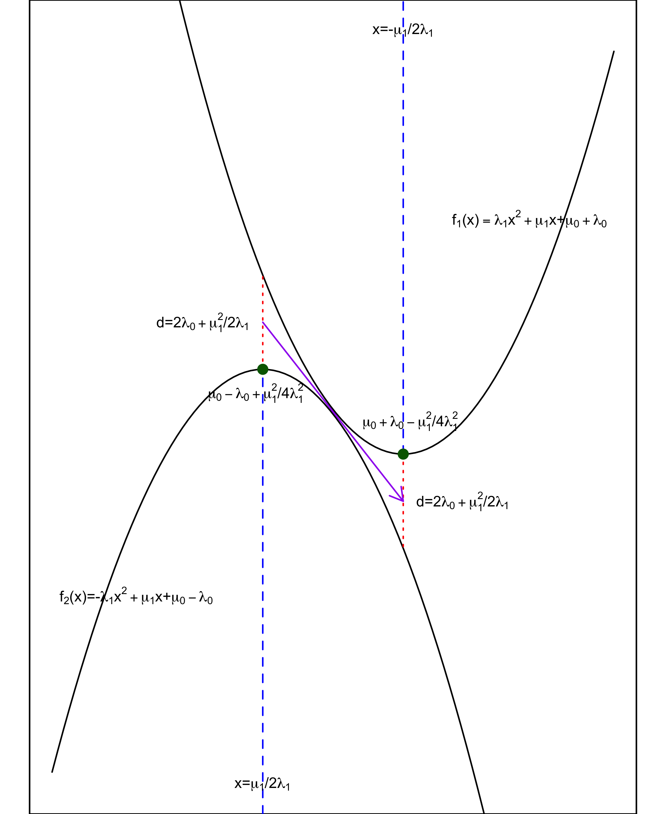
(a) Monotonically decreasing function.

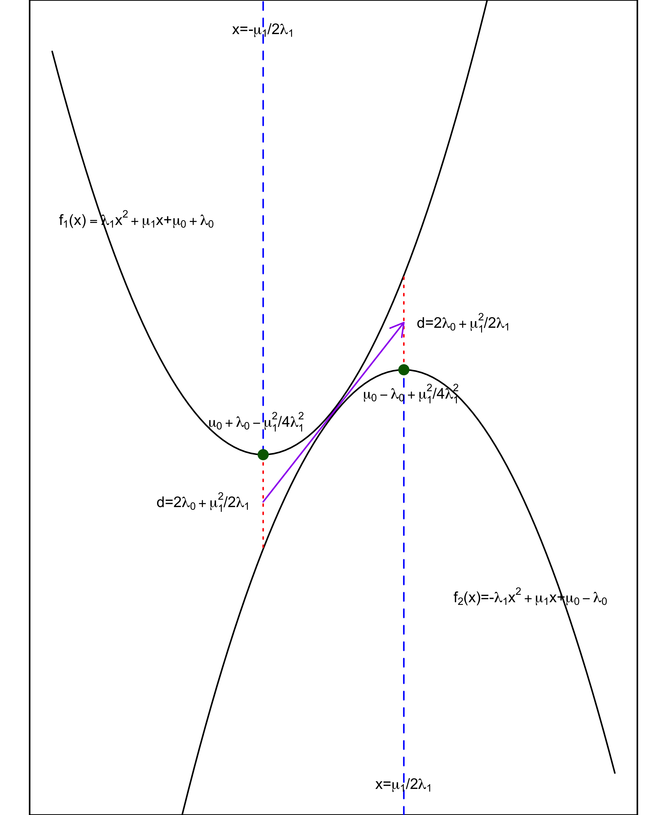
(b) Monotonically increasing function.

Figure S1: Illustration of how the two bounds can be used to set the monotonic pattern of the prior expected probability response curve.

Specifically, suppose the prior guess for the first probability response curve is a decreasing function with respect to $x$. As shown in Figure 1(a), we can put the range of $x$ inside the two axes of symmetry. In addition, the quantity $d=2\lambda_{0}+\mu_{1}^{2}/2\lambda_{1}$ determines the maximum difference of the two bounds. The two vertices determine the prior mean at the minimum and maximum value of $x$. To summarize, the parameters $\mu_{0},\mu_{1},\lambda_{0},\lambda_{1}$ can be specified by the equations

$$\left\{\begin{aligned} &\frac{\mu_{1}}{2\lambda_{1}}=a_{1},\quad-\frac{\mu_{1}}{2\lambda_{1}}=-a_{1}\\ &2\lambda_{0}+\frac{\mu_{1}^{2}}{2\lambda_{1}}=a_{2}\\ &\mu_{0}+\lambda_{0}-\frac{\mu_{1}^{2}}{4\lambda_{1}}=-a_{3}\\ &\mu_{0}-\lambda_{0}+\frac{\mu_{1}^{2}}{4\lambda_{1}}=a_{4}\end{aligned}\right.\Longleftrightarrow\left\{\begin{aligned} &\mu_{0}=\frac{a_{4}-a_{3}}{2}\\ &\mu_{1}=-\frac{a_{2}+a_{3}+a_{4}}{2a_{1}}\\ &\lambda_{0}=\frac{a_{2}-a_{3}-a_{4}}{4}\\ &\lambda_{1}=\frac{a_{2}+a_{3}+a_{4}}{4a_{1}^{2}}\end{aligned}\right.$$ (S1)

with positive numbers $a_{1},a_{2},a_{3},a_{4}$ choosing based on the prior information. Note that $\lambda_{0}$ should be positive, so it imposes the constraint $a_{2}>a_{3}+a_{4}$ on the choice of these four numbers. Using (S1), we can specific the prior hyperparameters $\mu_{01,0},\mu_{01,1},\lambda_{01,0},\lambda_{01,1}$. The same strategy can be extended for the monotonic increasing case.

To specify $\bm{\mu}_{0j}$ and $\Lambda_{0j}$ for $j>1$, we can sequentially implement this strategy. Furthermore, if the dimension of covariates $p>2$, it becomes more difficult to specify hyperparameters, but the same strategy can be applied by considering each covariate $x_{s},s=1,\cdots,p$ marginally while fixing $x_{s^{\prime}},s^{\prime}\neq s$.

We specify the prior hyperparameters of the illustrative example in Section 2.3 by the proposed strategy. Suppose the prior information we want to incorporate is $\text{Pr}(\mathbf{Y}=1\mid x)$ decreasing from 1 to 0 while $\text{Pr}(\mathbf{Y}=2\mid x)$ increasing from 0 to 1 in the region $(-10,10)$. For the first decreasing probability curve, we set $a_{1}=a_{2}=10,a_{3}=6,a_{4}=2$ to specify $\bm{\mu}_{01}$ and $\Lambda_{01}$. As for the second probability curve, since $\text{E}(\text{Pr}(\mathbf{Y}=2\mid G_{\mathbf{x}}))=[1-\text{E}(\text{Pr}(\mathbf{Y}=1\mid G_{\mathbf{x}}))]\text{E}[\varphi(\mathbf{x}^{T}\bm{\beta}_{2})]$ and utilizing the specified monotonicity for $\text{E}(\text{Pr}(\mathbf{Y}=1\mid G_{\mathbf{x}})))$, sequentially we focus on $\text{E}[\varphi(\mathbf{x}^{T}\bm{\beta}_{2})]$. To force a increasing trend, we further choose $\bm{\mu}_{02}$ and $\Lambda_{02}$ by applying the strategy for the increasing case with same setting on $a_{1}$ to $a_{4}$. After simple algebra we obtain prior hyperaprameters choice

$$\bm{\mu}_{01}=(-2,-0.9)^{T},\,\,\bm{\mu}_{02}=(-2,0.9)^{T},\,\,\Lambda_{01}=\Lambda_{02}=\begin{pmatrix}0.8&0\\ 0&0.072\end{pmatrix}$$

This set of prior hyperparameters lead to Figure 2.

S3 Additional results for data examples

S3.1 Synthetic data examples

First experiment

We perform a formal model comparison using the posterior predictive loss criterion (Gelfand and Ghosh, 1998). The criterion contains a goodness-of-fit term and a penalty term. Since the response variable $\mathbf{Y}$ is multivariate, we consider posterior predictive loss for every entry of it. Specifically, let $\mathbf{Y}_{i}^{*}$ denote the replicate response drawn from the posterior predictive distribution. Then, the goodness-of-fit term is defined as $G_{j}(\mathcal{M})=\sum_{i=1}^{n}[\mathbf{Y}_{ij}-\text{E}^{\mathcal{M}}(\mathbf{Y}^{*}_{ij}|\text{data})]^{2}$, whereas the penalty term is defined as $P_{j}(\mathcal{M})=\sum_{i=1}^{n}\text{Var}^{\mathcal{M}}(\mathbf{Y}^{*}_{ij}|\text{data})$, for $j=1,\cdots,C$. After fitting the three proposed models, we calculate posterior predictive loss with its two components. The results are summarized in Table S1. We also plot the posterior mean of the three largest weights and the corresponding atoms $\varphi(\theta_{1})$ and $\varphi(\theta_{2})$ in Figure S2. Combining with the posterior predictive loss criterion for each model, we can diagnose how the three models estimate the probability response curves. For similarities, it appears that all three models are dominated by the mixing component with the largest weight, whose shape is similar to the truth. (The common-weights model favors two mixing components, but the two components are close to each other.) For differences, the common-atoms model can only adjust the shape of regression lines through the mixing weights. It uses more effective mixing components with shapes differing dramatically, yielding larger goodness-of-fit and penalty terms. The general model is more effective in capturing the actual shape. It uses fewer and similar effective mixing components, leading to smaller penalty terms. In addition, the covariate effect is partly explained by the weights, causing slight bias compared to the common-weights model.

Table S1: First simulation example. Summary of model comparison using the posterior predictive loss criterion.

Model	$G_{1}(\mathcal{M})$	$P_{1}(\mathcal{M})$	$G_{2}(\mathcal{M})$	$P_{2}(\mathcal{M})$	$G_{3}(\mathcal{M})$	$P_{3}(\mathcal{M})$
Common-weights	6.94	7.94	12.95	13.59	8.41	9.00
Common-atoms	7.35	9.73	13.76	15.43	8.73	11.99
General	7.26	7.38	12.94	12.78	8.51	8.84

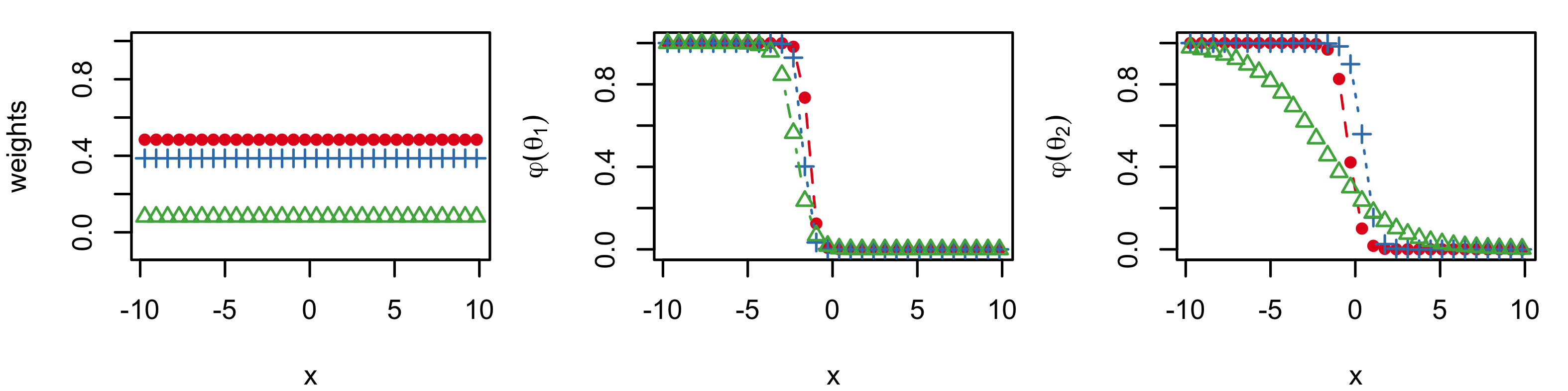
(a) Common-weigths model.

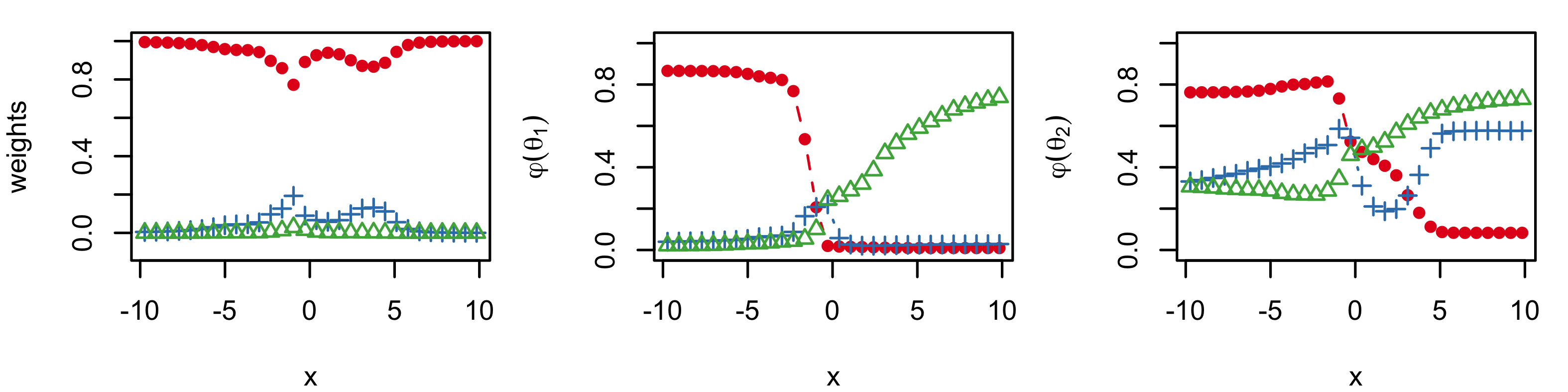
(b) Common-atoms model.

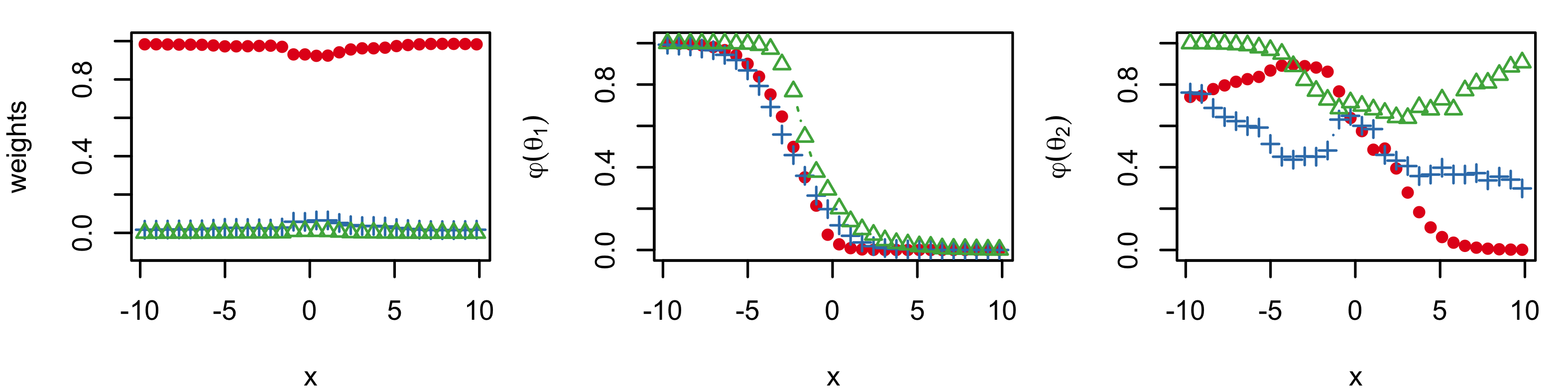
(c) General model.

Figure S2: First simulation example. Posterior mean estimates of the three largest mixing weights and atoms in estimating the probability response curves. The red circle, blue plus and green triangle correspond to the first to the third largest weights, respective.

Under the first experiment setting, the true probability response curves are known and have specific monotonic patterns. It would be interesting to see the models’ behavior if we specify the prior hyperparameters with more caution, such that the prior point and interval estimates of the probability response curves possess the true monotonicity. That is, we use the prior information that $Pr(\mathbf{Y}=1|x)$ decreasing from 1 to 0 and $Pr(\mathbf{Y}=3|x)$ increase from 0 to 1 in the region $(-10,10)$ to specify a more informative prior. Using the aforementioned prior specification strategy, the prior hyperparameters we use for the general model is

$$\bm{\mu}_{0j}=(-2,-0.9)^{T},\,\,\Lambda_{0j}=\begin{pmatrix}0.8&0\\ 0&0.072\end{pmatrix},\,\,j=1,2$$

and we set $\bm{\gamma}_{0}=(-2.5,0)$ and $\Gamma_{0}=diag(10,1)$ to favor a priori enough number of distinct components while keep the truncated model closely enough to the countable mixture model. The prior hyperparameters of the other two simplified models are specified accordingly. This set of prior hyperparameters leads to the posterior inference shown in Figure 5.

Second experiment

To illustrate the benefits of incorporating local, covariate-dependent weights in the nonparametric mixture model, we conduct the second experiment. The prior hyperparameters are specified deliberately, yielding fairly noninformative prior such that the three nonparametric models provide similar prior point and interval estimates of the probability response curves. As a consequence, the disparity in posterior estimates should be led by the difference in the mixing structure. More specifically, we set the LSBP prior hyperparameters $(\bm{\gamma}_{0},\Gamma_{0})$ to favor a priori enough mixture components over the covariate space. The hyperparameters $(a_{\alpha},b_{\alpha})$ in the common-weights model are set accordingly to favor a comparable number of mixing components. In addition, the hyperparameters corresponding to the atoms are set as the baseline choice. Figure S3 displays the prior point and interval estimates under the proposed models. The three subfigures display the same pattern: the prior mean estimate are flat, and the prior $95\%$ interval estimates span a substantial portion of the unit interval.

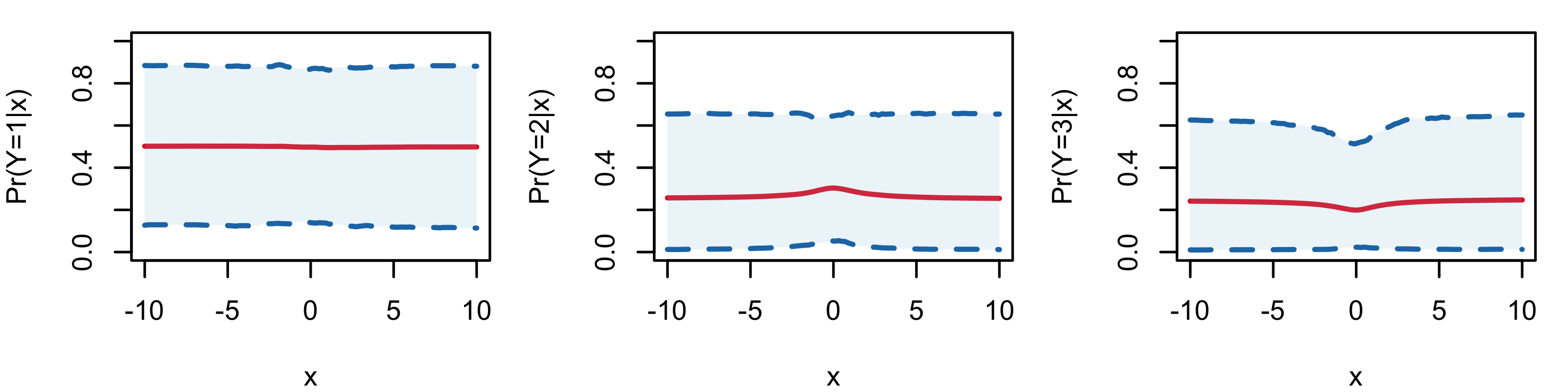
(a) Common-weights model.

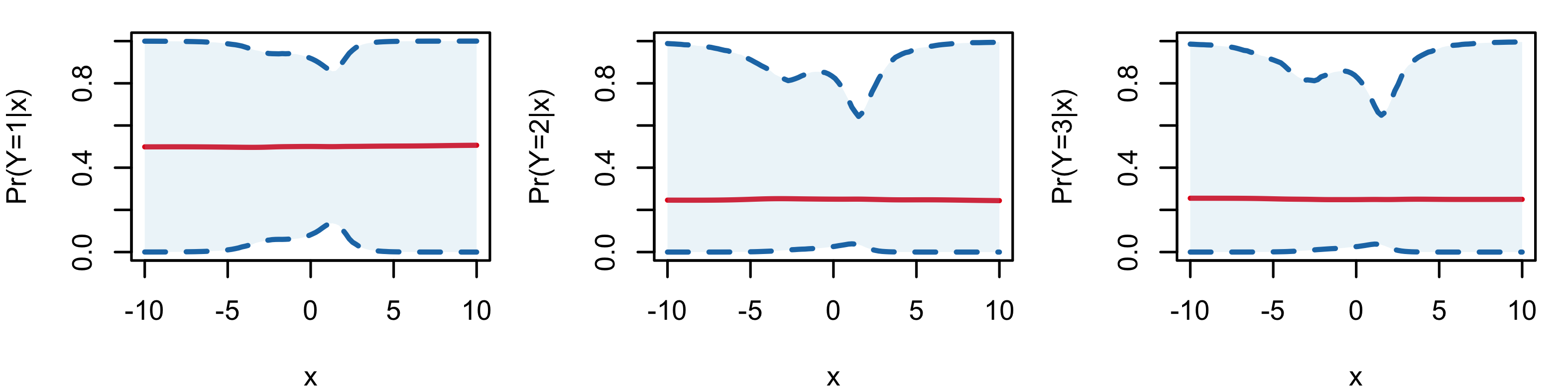
(b) Common-atoms model.

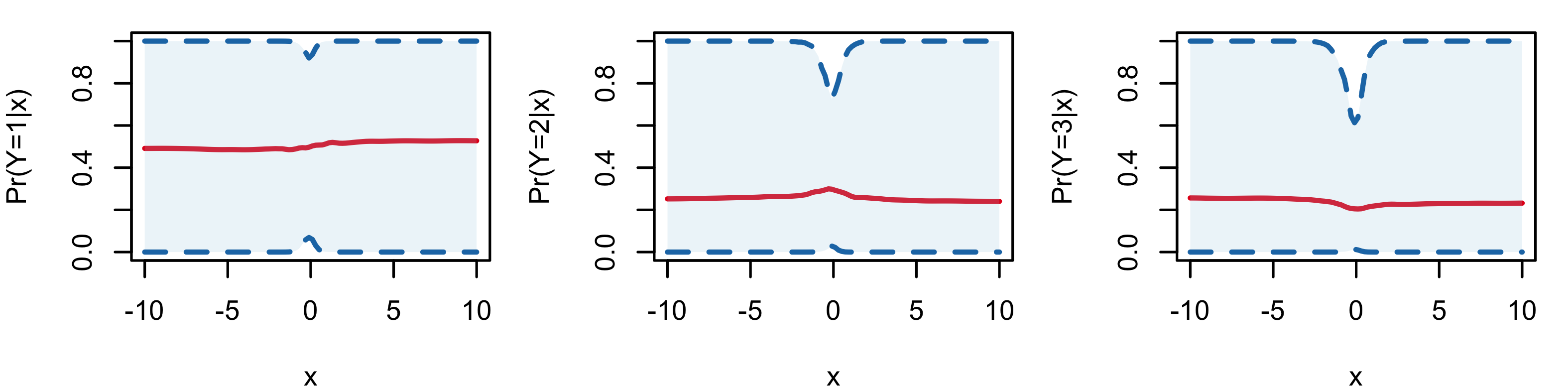
(c) General model.

Figure S3: Second simulation example. In each panel, the red solid line corresponds to the prior expected probability response curve, the blue dashed lines and shaded region indicate the prior 95% interval estimate.

Under the displayed prior, the posterior estimates are shown in Figure 6. The models with covariate-dependent weights learn the true probability regression function pattern from the data. In contrast, the common-weights model struggles when the regression curves behave locally atypical. Examining the results allows us to conclude that covariate-dependent weights are practically helpful in inferring the covariate-response relationship.

To further investigate how the proposed models behave in capturing non-standard probability response curves, we conduct a model comparison using the aforementioned posterior predictive loss criterion, with the result summarized in Table S2. Clearly, the two models with covariate-dependent weights outperform the common-weights model. The common-atoms model and the general model are comparable in terms of goodness of fit. Nonetheless, the common-atoms model activates more effectively components to compensate for the constant atoms in curve fitting, resulting in a larger penalty.

Table S2: Second simulation example. Summary of model comparison using the posterior predictive loss criterion.

Model	$G_{1}(\mathcal{M})$	$P_{1}(\mathcal{M})$	$G_{2}(\mathcal{M})$	$P_{2}(\mathcal{M})$	$G_{3}(\mathcal{M})$	$P_{3}(\mathcal{M})$
Common-weights	132.59	141.27	72.76	83.54	136.40	141.91
Common-atoms	90.52	103.84	65.79	82.25	89.45	107.64
General	89.96	96.25	64.14	72.56	88.24	94.39

S3.2 Credit ratings of U.S. firms

We first compare the posterior point estimates of the first-order marginal probability curves $\pi_{j}(x_{s})$, $j=1,\cdots,5$ and $s=1,\cdots,5$, obtained by the proposed nonparametric models and their parametric backbone. The results are shown in Figure LABEL:fig:compareallmodel. The continuation-ratio logits regression model contains fewer parameters than the nonparametric models, leading to reduced flexibility. As shown in Figure LABEL:subfig:conratiomargin, the estimated curves have a standard shape. In contrast, the flexible nature of the nonparametric models enables complicated regression relationships to be extracted from the data. To discuss the difference in the estimated regression trends regarding a certain covariate, consider the standardized log-sales variable as an example. For low to moderate log-sales values, the probability of the lowest rating level decreases at about the same rate under the continuation-ratio logits model, while the decreasing rate varies under the three nonparametric models. The latter pattern is more plausible.

A formal model comparison based on the posterior predictive loss criterion (definition provided in Section S3.1) is presented in Table S3. The common-weights model and the general model yield comparable results, while both models outperform the parametric model in predicting the probability of the first four credit levels. As for credit level 5, the three models are comparable regarding the goodness-of-fit criterion, while the nonparametric models yield larger penalty terms. We notice that there are substantially fewer firms with credit level 5, which may be the reason the nonparametric models provide larger penalty.

Table S3: Credit ratings data. Summary of the posterior predictive loss criteria for model comparison. Each pair of numbers corresponds to $(G_{j}(\mathcal{M}),P_{j}(\mathcal{M}))$, $j=1,\cdots,5$. The term “parametric” refers to the continuation-ratio logits model.

	Parametric	Common-weights	Common-atoms	General
Credit level 1	$(92.65,90.17)$	$(88.07,92.38)$	$(92.64,104.97)$	$(86.61,95.79)$
Credit level 2	$(158.71,158.72)$	$(153.13,158.92)$	$(156.04,163.96)$	$(153.10,158.07)$
Credit level 3	$(150.18,150.82)$	$(145.40,150.38)$	$(149.00,152.03)$	$(148.11,148.60)$
Credit level 4	$(95.95,96.29)$	$(95.08,97.23)$	$(97.41,100.10)$	$(94.20,94.24)$
Credit level 5	$(17.80,17.46)$	$(17.85,20.57)$	$(21.19,31.04)$	$(17.74,20.47)$

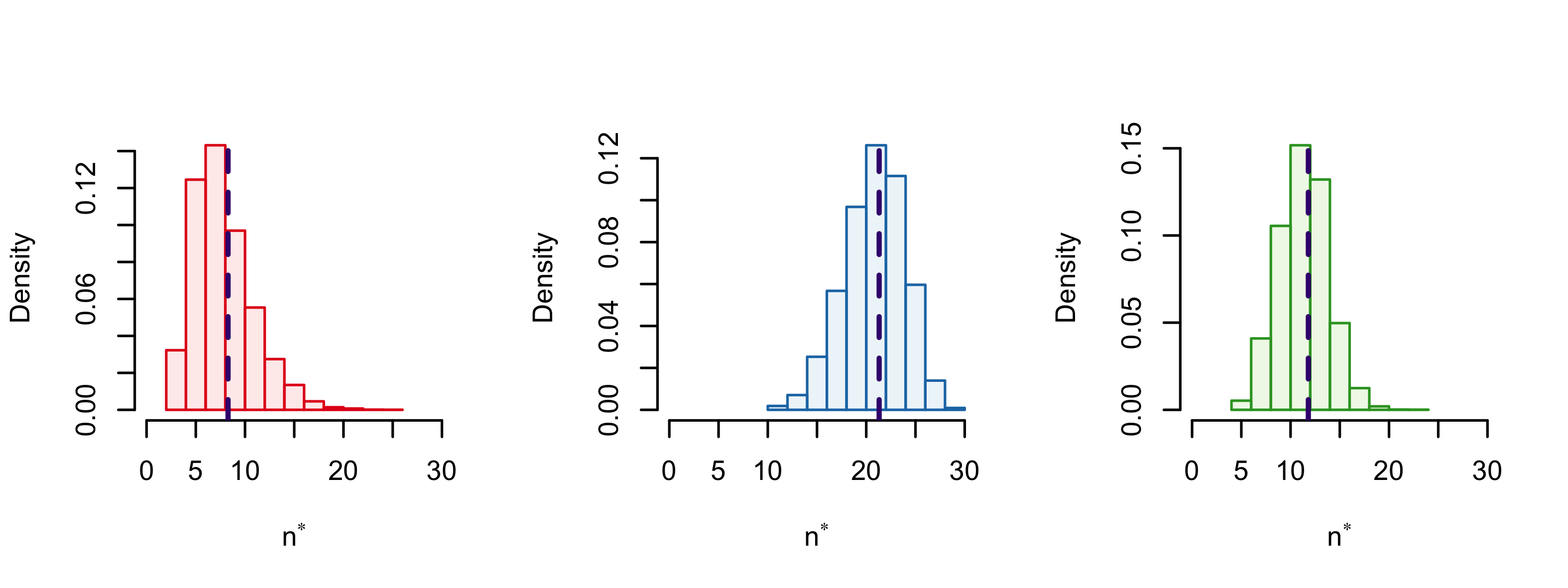
Figure S4: Credit ratings data. Posterior distributions for the number of distinct components. The purple dashed line indicates the posterior mean. The panels correspond to, from left to right, the common-weights model, the common-atoms model, and the general model, respectively.

We also notice the significantly larger penalty terms for the common-atoms model. This is to be expected, since the shape of the regression curves are only allowed to be adjusted through the mixing weights under the common-atoms model. Therefore, to provide regression curve estimates as in Figure LABEL:subfig:lsbpmargin, it should activate more mixing components. Figure S4 shows the posterior distribution for the number of distinct components under the three nonparametric models. It demonstrates that the common-atoms model suffers from overfitting in this specific example, leading to the larger penalty terms.

Furthermore, it is also of interest to investigate the model performance on prediction. The credit rating of firms can be partitioned into two categories: investment grade (rating score is 3 or higher) and speculative grade. Because many bond portfolio managers are not allowed to invest in speculative grade bonds, firms with a speculative rating incur significant costs. It is helpful to check the models’ implied posterior probability of obtaining an investment grade for a particular firm. We consider five prediction scenarios corresponding to the five covariates. In each scenario, we evaluate the change in the investment grade probability associated with one of the covariates changing from the 25th to the 75th percentile of the observed values, while holding all the other covariates at the average value of all observations. Figure S5 displays the posterior distribution of the probability of obtaining investment grade under the common-weights model.

Under the common-weights model, the probability moves along the expected direction concerning all covariates, except for the working capital, which coincides with the discovery in Verbeek (2008). The results indicate higher leverage, meaning that a firm is financed relatively more with debt, which reduces the expected credit rating. It is due to that firms with high leverage face substantially higher debt financing costs. In addition, the larger firms, indicated by larger log-sales, have significantly better credit ratings than smaller firms, ceteris paribus. Higher earnings before interest and taxes and higher retained earnings also improve credit ratings. Furthermore, one would expect that maintaining a high level of working capital would enhance a company’s credit rating since it reduces risk. However, a high level of working capital reduces profits, raising concern about the company’s ability to cover interest payments. This argument suggests a concave relationship between working capital and credit rating, postulating that firms could have an optimal working capital ratio. Our result indicates that the optimal ratio lies between the first and third quartiles.

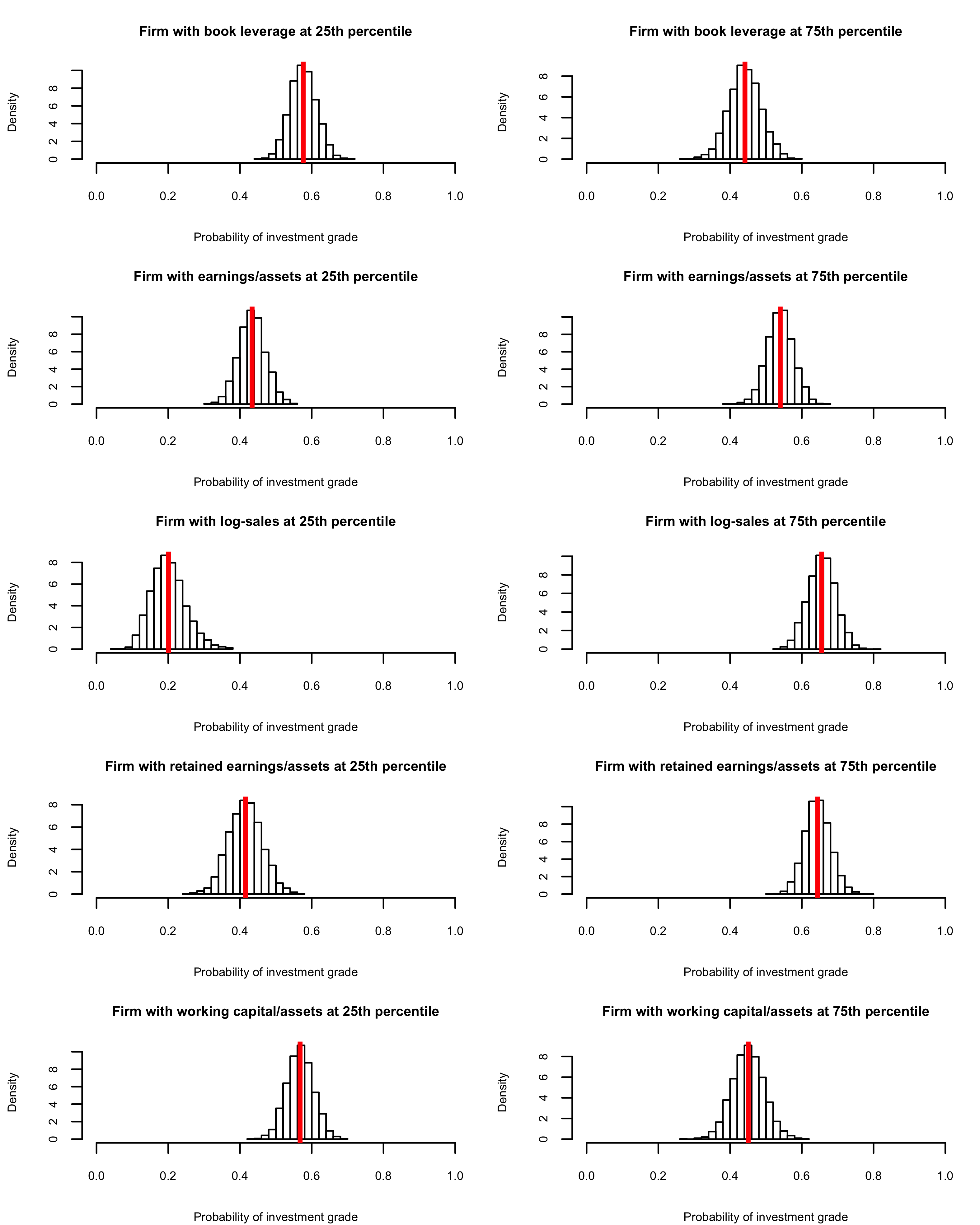
Figure S5: Credit ratings data. Posterior distributions of the probability of obtaining investment grade rating under the common-weights model. The red solid lines indicate the posterior mean.

S3.3 Developmental toxicology data example

We notice that, to ensure monotonicity of the prior expected dose-response curve, as pointed out by Fronczyk and Kottas (2014), we can restrict the support of $\beta_{j1}$, for $j=1,2$, to be $[0,\infty)$, using, for example, an exponential prior. However, that choice breaks the conjugacy in posterior full conditional distributions, complicating the posterior simulation procedure. We instead follow the procedure in Section S2 to choose the prior hyperparameters such that the non-decreasing trend is present in the prior expected dose-response curves. Indeed, the trend is strongly favored in individual priors realizations for the dose-response curves. This is a useful compromise, since it effectively achieves the practical goal of the monotonic trend, and at the same time, it retains the efficient posterior simulation method discussed in the paper. Figure S6 displays the prior expectation and interval estimates for the various dose-response curves under the specified prior hyperparameters, together with 5 prior realizations.

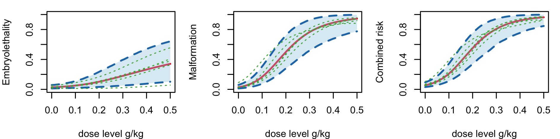
(a) Common-weights model.

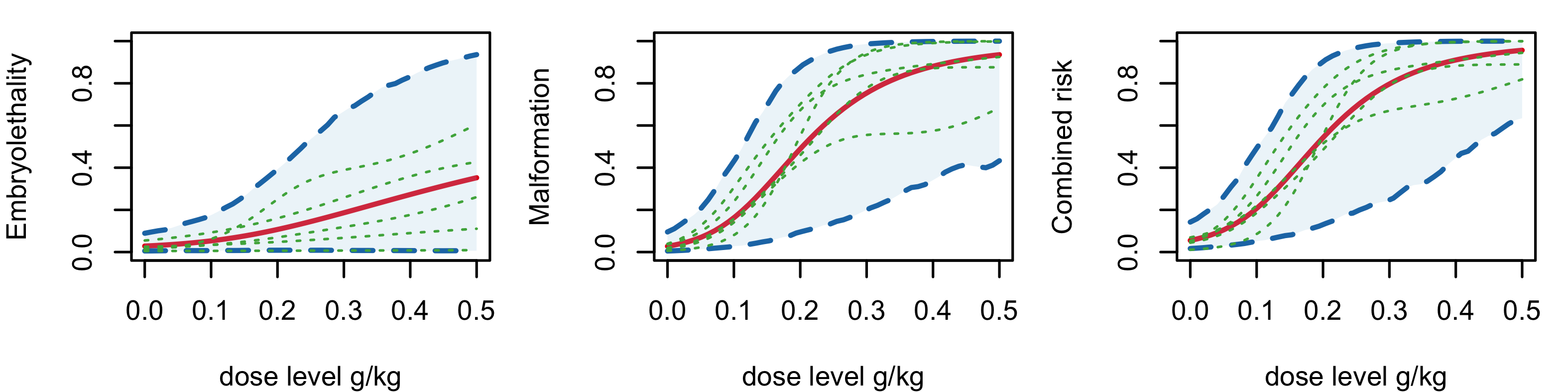
(b) General model.

Figure S6: DYME data. In each panel, the red solid line corresponds to the prior expected probability response curve, the blue dashed lines and shaded region indicate the prior 95% interval estimate, and the green dotted lines show 5 prior realizations.

We consider model comparison based on the posterior predictive loss criterion applied to each of the endpoints. Let $d=1,\cdots,n_{i}$ index the dams at observed dose level $x_{i}$, for $i=1,\cdots,N$. At each iteration, we draw one set of posterior predictive sample at each observed dose level, denoted as $m_{i}^{*}$, $R_{i}^{*}$ and $y_{i}^{*}$. This is because the responses from the $n_{i}$ dams at the $i$th dose level share the same covariate $\mathbf{x}_{i}$. For each endpoint, the criterion favors the model $\mathcal{M}$ that minimizes both a goodness-of-fit term $G(\mathcal{M})$, and a penalty term for model complexity $P(\mathcal{M})$. Specifically, for the embryolethality endpoint, we define $G(\mathcal{M})=$ $\sum_{i=1}^{N}\sum_{d=1}^{n_{i}}\{R_{id}/m_{id}-\text{E}(R_{i}^{*}/m_{i}^{*}\mid\text{data})\}^{2}$, and the penalty term is defined as $P(\mathcal{M})=$ $\sum_{i=1}^{N}n_{i}\text{Var}(R_{i}^{*}/m_{i}^{*}\mid\text{data})$. These two terms are defined analogously for the other two endpoints, based on posterior predictive samples $y_{i}^{*}/(m_{i}^{*}-R_{i}^{*})$ and $(R_{i}^{*}+y_{i}^{*})/m_{i}^{*}$. The results, reported in Table S4, favor the general model.

Table S4: Values for the two terms of the posterior predictive loss criterion for each endpoint. The bold values are for the general model while the numbers inside the bracket are for the common-weights model.

Endpoint	$G(\mathcal{M})$	$P(\mathcal{M})$
Embryolethality	2.140  (2.185)	2.015  (2.258)
Malformation	1.720  (1.714)	1.626  (2.325)
Combined risk	1.946  (1.955)	1.412  (1.969)

The posterior estimates of the dose-response curves under the common-weights model and the general model are shown in Figure S7 and Figure 11 (in the main manuscript), respectively. Contrasting with the prior estimate presented in Figure S6, there is substantial learning for the proposed models as the posterior estimate is significantly concentrated relative to the corresponding prior estimate.

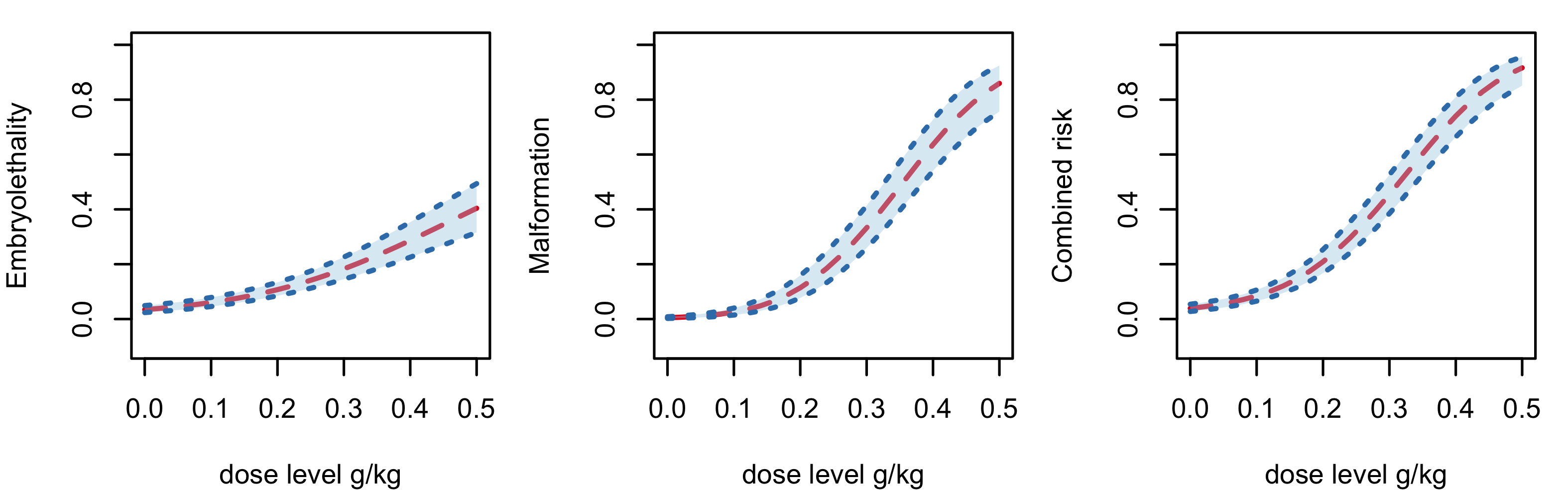
Figure S7: DYME data. Posterior point and interval estimate of the dose-response curves under the common-weights model. The red dashed line denotes the posterior mean while the blue dotted line and shaded region represent the posterior 95$\%$ credible interval estimate.

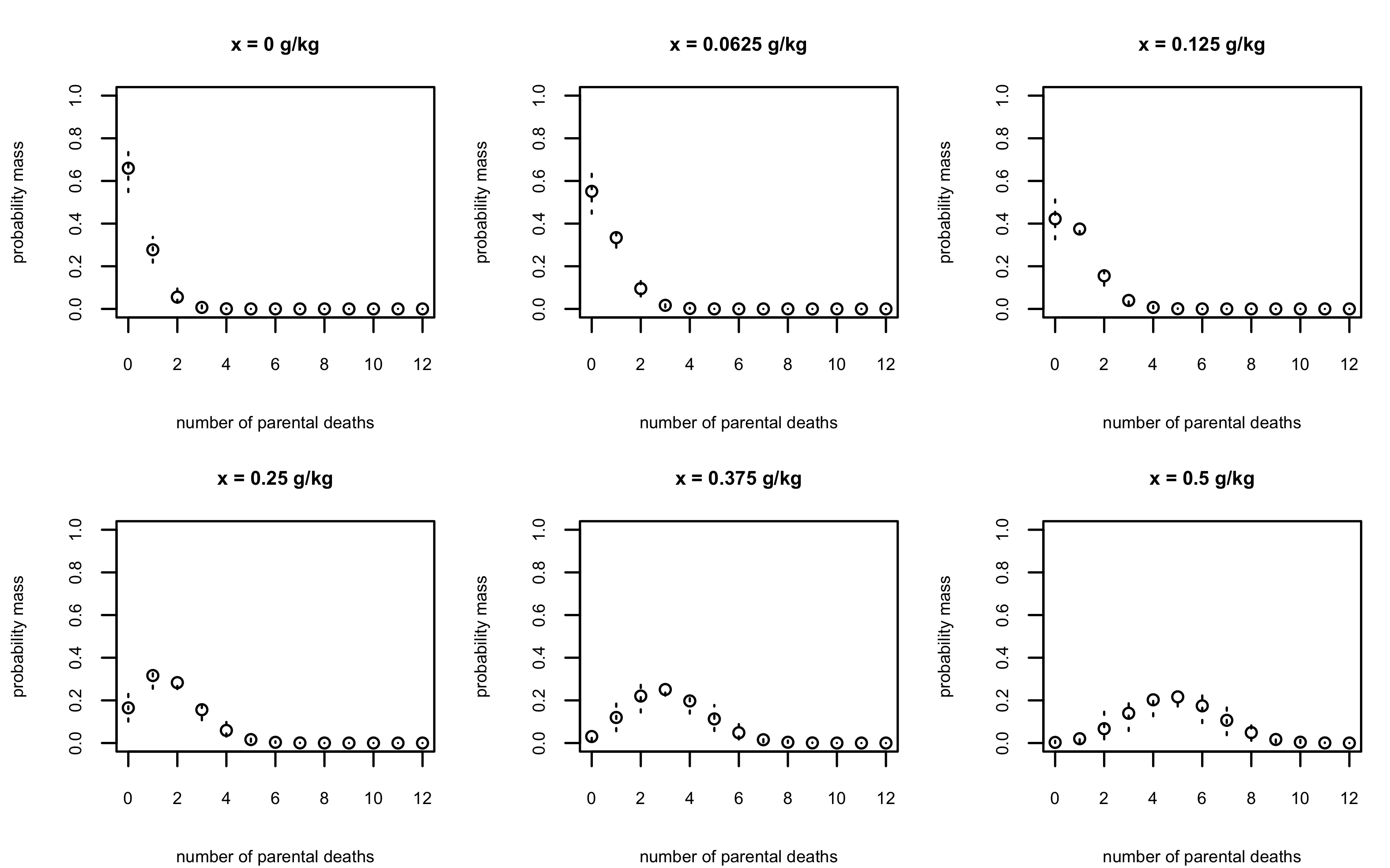
(a) The common-weights model.

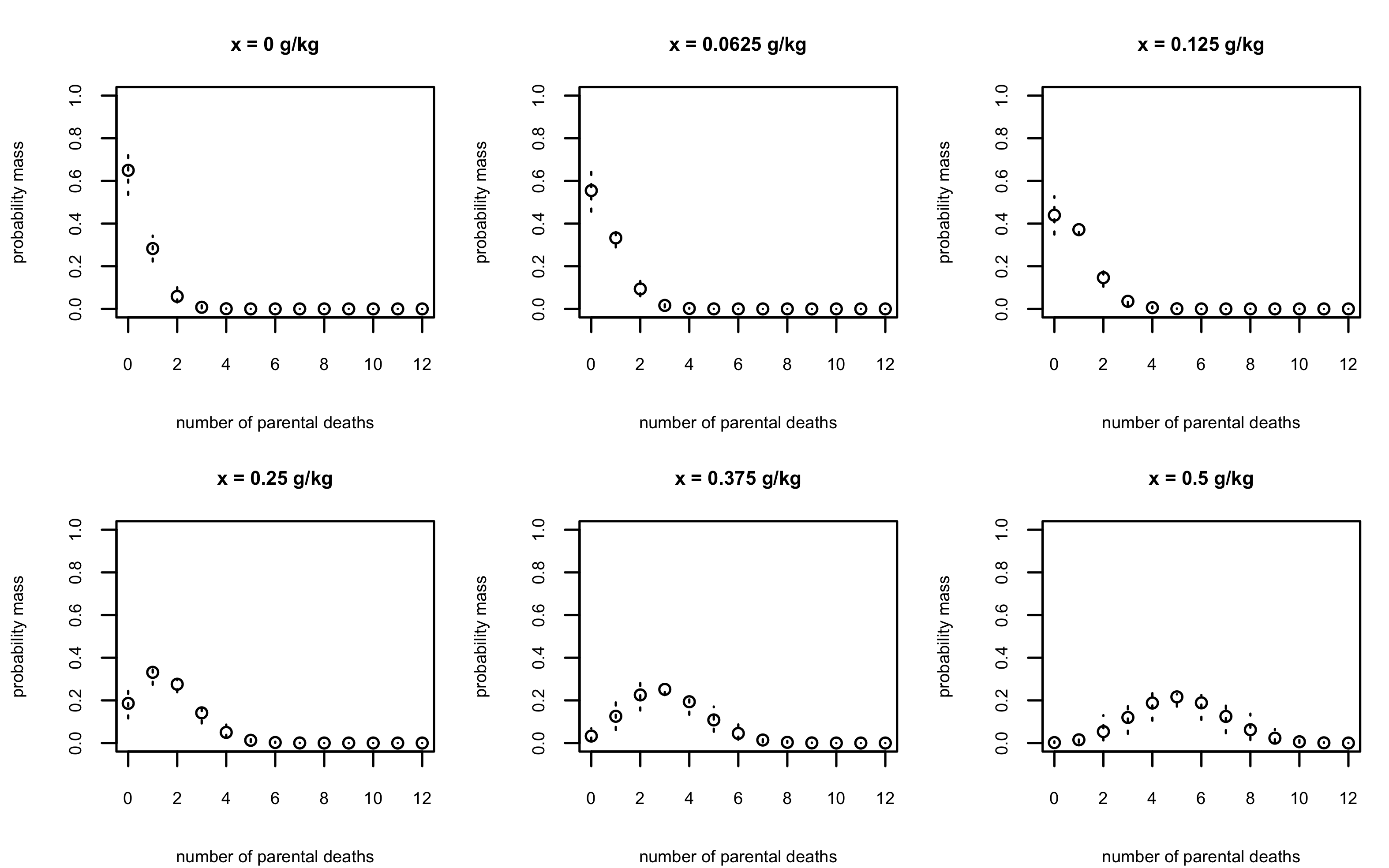
(b) The general model.

Figure S8: DYME data. Posterior mean (“o”) and 95$\%$ uncertainty bands (dotted lines) for the probability mass function associated with the number of non-viable fetuses given $m=12$ implants, $p(R\mid m=12,G_{\mathbf{x}})$, under two models. Results are shown for the five observed toxin levels and for the new value of $x=0.375$ g/kg.

We also study the probability mass functions under the common-weights and general models. Figure S8 displays estimates for the probability mass functions corresponding to the number of non-viable fetuses given a specific number of implants. Similar to the Figure 12 in the main manuscript, Figure S9 displays estimates for the conditional probability mass functions of the number of malformations given a specified number of implants and the associated number of non-viable fetuses under the common-weights model. The common-weights model and the general model provide comparable results. These results demonstrate that the proposed models can effectively estimate response distributions with different shapes across different toxin levels.

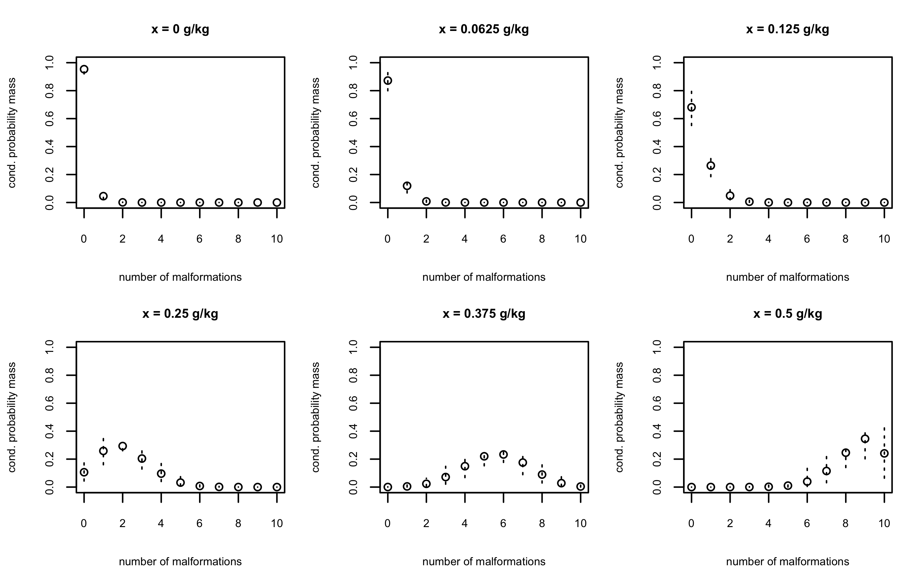
Figure S9: DYME data. Posterior mean (“o”) and 95$\%$ uncertainty bands (dotted lines) for the conditional probability mass function associated with the number of malformations given $m=12$ implants and $R=2$ non-viable fetuses, $p(y\mid m=12,R=2,G_{\mathbf{x}})$, under the common-weights model. Results are shown for the five observed toxin levels and for the new value of $x=0.375$ g/kg.

For the the general model, we perform model checking by cross-validation. We use one randomly chosen sample comprising data from 20 dams (approximately 20$\%$ of the data) spread roughly evenly across the dose levels as the test set. After fitting the general model to the reduced DYME data, we obtain for each observed toxin level posterior predictive samples for $R^{*}/m^{*},y^{*}/(m^{*}-R^{*})$ and $(R^{*}+y^{*})/m^{*}$. Figure S10, which displays box plots of these samples along with the corresponding values from the cross-validation data points, does not show evidence of ill-fitting.

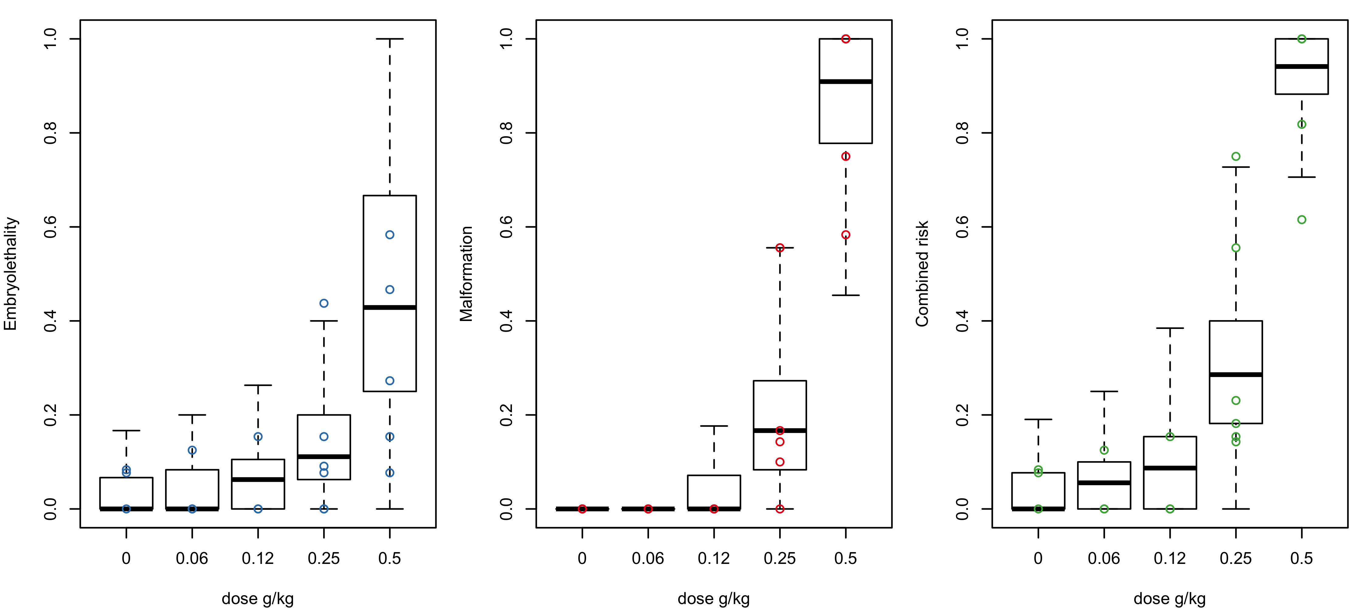
Figure S10: Box plots of posterior predictive samples for the embryolethality (left panel), malformation (middle panel), and combined risk (right panel) endpoint at the observed toxin levels. The corresponding values from the 20 cross-validation data points are denoted by "o".

References

- Agresti (2012) Agresti, A. (2012), Categorical Data Analysis, Wiley Series in Probability and Statistics, Hoboken, NJ, USA: Wiley.
- Albert and Chib (1993) Albert, J. H. and Chib, S. (1993), “Bayesian Analysis of Binary and Polychotomous Response Data,” Journal of the American Statistical Association, 88, 669–679.
- Bao and Hanson (2015) Bao, J. and Hanson, T. (2015), “Bayesian Nonparametric Multivariate Ordinal Regression,” Canadian Journal of Statistics, 43, 337–357.
- Basu and Chib (2003) Basu, S. and Chib, S. (2003), “Marginal Likelihood and Bayes Factors for Dirichlet Process Mixture Models,” Journal of the American Statistical Association, 98, 224–235.
- Blei and Jordan (2006) Blei, D. M. and Jordan, M. I. (2006), “Variational Inference for Dirichlet Process Mixtures,” Bayesian Analysis, 1, 121–143.
- Blei et al. (2017) Blei, D. M., Kucukelbir, A., and McAuliffe, J. D. (2017), “Variational Inference: A Review for Statisticians,” Journal of the American Statistical Association, 112, 859–877.
- Boes and Winkelmann (2006) Boes, S. and Winkelmann, R. (2006), “Ordered Response Models,” Allgemeines Statistisches Archiv, 90, 167–181.
- Chib and Greenberg (2010) Chib, S. and Greenberg, E. (2010), “Additive Cubic Spline Regression with Dirichlet Process Mixture Errors,” Journal of Econometrics, 156, 322–336.
- Choudhuri et al. (2007) Choudhuri, N., Ghosal, S., and Roy, A. (2007), “Nonparametric Binary Regression Using a Gaussian Process Prior,” Statistical Methodology, 4, 227–243.
- DeIorio et al. (2009) DeIorio, M., Johnson, W. O., Müller, P., and Rosner, G. L. (2009), “Bayesian Nonparametric Nonproportional Hazards Survival Modeling,” Biometrics, 65, 762–771.
- DeIorio et al. (2004) DeIorio, M., Müller, P., Rosner, G. L., and MacEachern, S. N. (2004), “An ANOVA Model for Dependent Random Measures,” Journal of the American Statistical Association, 99, 205–215.
- DeYoreo and Kottas (2018) DeYoreo, M. and Kottas, A. (2018), “Bayesian Nonparametric Modeling for Multivariate Ordinal Regression,” Journal of Computational and Graphical Statistics, 27, 71–84.
- DeYoreo and Kottas (2020) — (2020), “Bayesian Nonparametric Density Regression for Ordinal Responses,” in Fan, Y., Nott, D., Smith, M. S., and Dortet-Bernadet, J.-L. (editors), Flexible Bayesian Regression Modelling, Academic Press, 65–90.
- Dunson and Park (2008) Dunson, D. B. and Park, J.-H. (2008), “Kernel stick-breaking processes,” Biometrika, 95, 307–323.
- Dunson and Rodríguez (2011) Dunson, D. B. and Rodríguez, A. (2011), “Nonparametric Bayesian Models through Probit Stick-breaking Processes,” Bayesian Analysis, 6, 145–177.
- Ferguson (1973) Ferguson, T. S. (1973), “A Bayesian Analysis of Some Nonparametric Problems,” The Annals of Statistics, 1, 209–230.
- Fronczyk and Kottas (2014) Fronczyk, K. and Kottas, A. (2014), “A Bayesian Nonparametric Modeling Framework for Developmental Toxicity Studies (with discussion),” Journal of the American Statistical Association, 109, 873–893.
- Gelfand and Ghosh (1998) Gelfand, A. E. and Ghosh, S. K. (1998), “Model choice: A Minimum Posterior Predictive Loss Approach,” Biometrika, 85, 1–11.
- Gelfand et al. (2005) Gelfand, A. E., Kottas, A., and MacEachern, S. N. (2005), “Bayesian Nonparametric Spatial Modeling With Dirichlet Process Mixing,” Journal of the American Statistical Association, 100, 1021–1035.
- Ishwaran and James (2001) Ishwaran, H. and James, L. F. (2001), “Gibbs Sampling Methods for Stick-Breaking Priors,” Journal of the American Statistical Association, 96, 161–173.
- Kottas and Fronczyk (2013) Kottas, A. and Fronczyk, K. (2013), “Flexible Bayesian modelling for clustered categorical responses in developmental toxicology,” in Damien, P., Dellaportas, P., Polson, N. G., and Stephens, D. A. (editors), Bayesian Theory and Applications, Oxford, UK: Oxford University Press, 70–83.
- Linderman et al. (2015) Linderman, S., Johnson, M. J., and Adams, R. P. (2015), “Dependent Multinomial Models Made Easy: Stick-Breaking with the Pólya-gamma Augmentation,” in Proceedings of the 28th International Conference on Neural Information Processing Systems - Volume 2, Cambridge, MA, USA: MIT Press.
- MacEachern (2000) MacEachern, S. N. (2000), “Dependent Dirichlet processes,” Technical report, Department of Statistics, The Ohio State University.
- Pirjol (2013) Pirjol, D. (2013), “The Logistic-normal Integral and Its Generalizations,” Journal of Computational and Applied Mathematics, 237, 460–469.
- Polson et al. (2013) Polson, N. G., Scott, J. G., and Windle, J. (2013), “Bayesian Inference for Logistic Models Using Pólya-Gamma Latent Variables,” Journal of the American Statistical Association, 108, 1339–1349.
- Price et al. (1987) Price, C. J., Kimmel, C. A., George, J. D., and Marr, M. C. (1987), “The Developmental Toxicity of Diethylene Glycol Dimethyl Ether in Mice,” Toxicological Sciences, 8, 115–126.
- Quintana et al. (2022) Quintana, F. A., Müller, P., Jara, A., and MacEachern, S. N. (2022), “The Dependent Dirichlet Process and Related Models,” Statistical Science, 37, 24–41.
- Rigon and Durante (2021) Rigon, T. and Durante, D. (2021), “Tractable Bayesian Density Regression via Logit Stick-breaking Priors,” Journal of Statistical Planning and Inference, 211, 131–142.
- Saarela et al. (2022) Saarela, O., Rohrbeck, C., and Arjas, E. (2022), “Bayesian Non-Parametric Ordinal Regression Under a Monotonicity Constraint,” Bayesian Analysis, 1–29.
- Tutz (1991) Tutz, G. (1991), “Sequential Models in Categorical Regression,” Computational Statistics and Data Analysis, 11, 275–295.
- Verbeek (2008) Verbeek, M. (2008), A guide to modern econometrics, Hoboken, NJ, USA: Wiley, 3rd ed. edition.