Dynamic Sensor Placement Based on Graph Sampling Theory

Abstract

In this paper, we consider a dynamic sensor placement problem where sensors can move within a network over time. Sensor placement problem aims to select $M$ sensor positions from $N$ candidates where $M<N$. Most existing methods assume that sensors are static, i.e., they do not move, however, many mobile sensors like drones, robots, and vehicles can change their positions over time. Moreover, underlying measurement conditions could also be changed that are difficult to cover the statically placed sensors. We tackle the problem by allowing the sensors to change their positions in their neighbors on the network. Based on a perspective of dictionary learning, we sequentially learn the dictionary from a pool of observed signals on the network based on graph sampling theory. Using the learned dictionary, we dynamically determine the sensor positions such that the non-observed signals on the network can be best recovered from the observations. Furthermore, sensor positions in each time slot can be optimized in a decentralized manner to reduce the calculation cost. In experiments, we validate the effectiveness of the proposed method via the mean squared error (MSE) of the reconstructed signals. The proposed dynamic sensor placement outperforms the existing static ones both in synthetic and real data.

Dynamic sensor placement on graphs, dictionary, sparse coding, graph sampling theory

1 INTRODUCTION

Sensor networks are used in various engineering applications such as traffic, infrastructure, and facility monitoring systems [1, 2, 3, 4]. They aim to efficiently collect information from distributed sensor measurements. Sensing targets include many environmental and/or behavioral data like temperature and acceleration [5, 6].

Sensor placement problem is one of the main research topics in sensor networks [7, 8, 9, 10]. Its purpose is to find $M$ sensor positions among $N$ candidates $(M<N)$ where sensors can be placed optimally so that the reconstruction error is minimized in some sense. It has been extensively studied in machine learning and signal processing [11, 12, 9, 13].

By placing sensors at appropriate positions, sensing costs, e.g., the number of sensors and the power consumption, can be significantly reduced. In this paper, we assume that candidate positions are given by nodes of a sensor network, i.e., a graph. This problem is considered as sensor placement problem for signals on the graph—graph signals.

The performance of the sensor placement is typically evaluated based on the reconstruction error from $M$ measurements [14, 9, 15, 16, 17, 18]. It depends on the quality of the dictionary used for reconstruction. Therefore, the dictionary design plays a key role in the sensor placement problem. From a dictionary learning perspective, existing sensing algorithms fall into two categories as follows [6]:

1. Compressed sensing (CS) using predefined basis functions [19, 20, 21]: The sensing process in CS is often random and determined independently of the dictionary. The dictionary in CS is typically selected from widely-used linear transforms like wavelets and the discrete cosine transform [6].

2. Data-driven sensing using bases learned from observations [6, 22]: It typically determines the sensor positions based on the dictionary. This leads to that its performance strongly depends on the quality of the designed dictionary. The basis is often set to principal vectors in the training data with the principal component analysis (PCA) or singular value decomposition (SVD) [22].

Hereafter, we consider the data-driven sensing, since it is known that it requires fewer sensors than the CS-based approach to achieve the same reconstruction performance [6].

Many existing works of sensor placement problem assume the static sensor placement, i.e., sensors do not or cannot be moved [23, 24, 25]. This leads to a limitation where we need to use the fixed dictionary when the dictionary has been once learned. However, the measurement conditions could be changed over time. In this case, the selected sensors in the static positions do not reflect the current signal statistics. This may lead to the limitation of reconstruction qualities.

To resolve the above-mentioned static sensor placement, we propose a sensor placement problem where sensors can flexibly change their positions over time. Typically, we consider a dynamic placement: Sensors that can move dynamically like drones and robots. For realizing the dynamic sensor placement, we sequentially learn the dictionary from a pool of observed graph signals by utilizing sparse coding. We then dynamically determine the sensor positions such that the non-observed graph signal can be best recovered from the sampled graph signal in every time instance. Furthermore, the sensor positions can be optimized in a decentralized manner to reduce their optimization and communication costs. In experiments, we demonstrate that the proposed method outperforms existing sensor placement methods both in synthetic and real datasets.

Notation: The notation of this paper is summarized in Table 1. We consider a weighted undirected graph $\mathcal{G}=(\mathcal{V,E})$, where $\mathcal{V}$ and $\mathcal{E}$ represent sets of nodes and edges, respectively. The number of nodes is $N=|\mathcal{V}|$ unless otherwise specified. The adjacency matrix of $\mathcal{G}$ is denoted by $\mathbf{W}$ where its $(m,n)$-element $[\mathbf{W}]_{mn}\geq 0$ is the edge weight between the $m$th and $n$th nodes; $[\mathbf{W}]_{mn}=0$ for unconnected nodes. The degree matrix $\mathbf{D}$ is defined as $\mathbf{D}=\text{diag}\,(d_{0},d_{1},\ldots,d_{N-1})$, where $d_{m}=\sum_{n}[\mathbf{W}]_{mn}$ is the $m$th diagonal element. We use graph Laplacian $\mathbf{L}\coloneqq\mathbf{D}-\mathbf{W}$ as a graph variation operator. A graph signal $\mathbf{x}\in\mathbb{R}^{N}$ is defined as a function $x[n]:\mathcal{V}\rightarrow\mathbb{R}$. Simply speaking, $x[n]$ is located on the node $n\in\mathcal{V}$ of $\mathcal{G}$.

The graph Fourier transform (GFT) of $\mathbf{x}$ is defined as

$$\hat{x}(\lambda_{i})=\braket{\mathbf{u}_{i},\mathbf{x}}=\sum_{n=0}^{N-1}u_{i}[n]x[n],$$ (1)

where $\mathbf{u}_{i}$ is the $i$th column of an orthonormal matrix $\mathbf{U}$ and it is obtained by the eigendecomposition of the graph Laplacian $\mathbf{L}=\mathbf{U\Lambda U}^{\top}$ with the eigenvalue matrix $\mathbf{\Lambda}=\mathrm{diag}\,(\lambda_{0},\lambda_{1},$ $\ldots,\lambda_{N-1})$. We refer to $\lambda_{i}$ as a graph frequency.

2 GRAPH SIGNAL SAMPLING

In this section, we introduce graph signal sampling. We first review graph sampling theory, and a sampling set selection on graphs [26] is then reviewed.

2.1 SAMPLING THEORY ON GRAPHS

Suppose that a graph signal is characterized by the following model

$$\mathbf{x}\coloneqq\mathbf{A}\mathbf{d},$$ (2)

where $\mathbf{A}\in\mathbb{R}^{N\times K}\ (K\leq N)$ is a known generator matrix and $\mathbf{d}\in\mathbb{R}^{K}$ are expansion coefficients. The generator matrix $\mathbf{A}$ specifies the signal subspace $\mathcal{A}$.

Table 1: Notation used in this paper.

$N$	Number of nodes
$K$	Number of sensors
$T$	Time duration (date length)
$D$	Number of time slots
$t$	Index of the time instance
$\|\cdot\|$	$\ell_{2}$ norm
$\|\cdot\|_{1}$	$\ell_{1}$ norm
$\|\cdot\|_{F}$	Frobenius norm
$\mathbf{Y}_{:i}$	$i$th column of $\mathbf{Y}$
$\mathbf{Y}_{xy}$	$(xy)$th element of $\mathbf{A}$
$\mathbf{Y}_{\mathcal{XY}}$	Submatrix of $\mathbf{Y}$ indexed by $\mathcal{X}$ and $\mathcal{Y}$
$\mathbf{Y}_{\mathcal{X}}$	$\mathbf{Y}_{\mathcal{XX}}$
$\mathcal{X}^{c}$	Complement set of $\mathcal{X}$
$\mathcal{R}(\mathbf{Q})$	Range space of $\mathbf{Q}$

The bandlimited (BL) model is one of the well-studied generator [27, 28, 29, 30, 31, 32], which is defined as

$$\mathbf{x}=\sum_{i=0}^{B-1}d[i]\mathbf{u}_{i}=\mathbf{U}_{\mathcal{VB}}\mathbf{d},$$ (3)

where $\mathbf{U}_{\mathcal{VB}}\in\mathbb{R}^{N\times B}$ is the submatrix of $\mathbf{U}$ whose rows are extracted within $\mathcal{B}=\{1,\ldots,B\}$ and $B$ is the bandwidth. In this case, $\mathbf{A}=\mathbf{U}_{\mathcal{VB}}$.

Piecewise constant (PC) model [33] is another possible signal model and is defined as follows.

$$\mathbf{x}=\sum_{i=1}^{C}d_{i}\mathbf{1}_{\mathcal{T}_{i}}=[\mathbf{1}_{\mathcal{T}_{1}},\dots,\mathbf{1}_{\mathcal{T}_{C}}]\mathbf{d},$$ (4)

where $\mathcal{T}_{k}\,(k=1,\ldots,K)$ is the nonoverlapping subset of nodes for the $k$th cluster: $[\mathbf{1}_{\mathcal{T}_{i}}]_{n}=1$ when the node $n$ is in $\mathcal{T}_{i}$ and $0$ otherwise [33].

If we do not know the exact $\mathbf{A}$ but have its prior knowledge, it needs to be learned from the observation. Let $\mathbf{X}\in\mathbb{R}^{N\times D}$ be a collection of $D$ graph signals. Typically, $\mathbf{A}$ has been determined by $\mathbf{A}=\bm{\mathcal{U}}$, where $\bm{\mathcal{U}}$ is obtained by the singular value decomposition (SVD) of the collection of observed signals $\mathbf{X}\coloneqq\bm{\mathcal{U}}\mathbf{\Sigma}\bm{\mathcal{V}}^{\top}$ [22].

Let $\mathbf{S}^{\top}\in\mathbb{R}^{K\times N}(K\leq N)$ be an arbitrary linear sampling operator. It specifies the sampling subspace $\mathcal{S}$. A sampled graph signal is represented by $\mathbf{c}=\mathbf{S}^{\top}\mathbf{x}$. The sampled signal is best recovered by the following transform [34, 35, 36]:

$$\tilde{\mathbf{x}}=\mathbf{A}\mathbf{H}\mathbf{c}=\mathbf{A}(\mathbf{S}^{\top}\mathbf{A})^{\dagger}\mathbf{c},$$ (5)

where $\cdot^{\dagger}$ is the Moore-Penrose pseudo-inverse. Here, $\mathbf{H}=(\mathbf{S}^{\top}\mathbf{A})^{\dagger}$ is referred to as the correction transform in generalized sampling [27]. If $\mathcal{A}$ and $\mathcal{S}$ together span $\mathbb{R}^{N}$ and only intersect at the origin, perfect recovery, i.e., $\tilde{\mathbf{x}}=\mathbf{x}$, is obtained. This implies that $\mathbf{S}^{\top}\mathbf{A}=\mathbf{H}$ is invertible. The invertibility of $\mathbf{H}$ is referred to as the direct sum (DS) condition [27].

In the above-mentioned sampling and reconstruction, $\mathbf{A}$ in (2) is assumed to be fixed. However, in general, $\mathbf{A}$ could be changed over time. In this paper, we consider the following time-varying generator:

$$\mathbf{x}_{t}=\mathbf{A}_{t}\mathbf{d}_{t},$$ (6)

where $\mathbf{A}_{t}$ and $\mathbf{d}_{t}$ are the generator and expansion coefficients at time $t$, respectively. In this paper, we infer $\mathbf{A}_{t}$ from $D$ observations

$$\mathbf{X}_{t-1}=[\mathbf{x}_{t-D-1},\dots,\mathbf{x}_{t-1}]$$ (7)

in every time instance for dynamic sensor placement.

From a perspective of the sensor placement, $\mathbf{S}^{\top}$ can be considered as a node-wise sampling operator $\mathbf{S}^{\top}=\{0,1\}^{K\times N}$. In the following, we introduce a node-wise sampling method on $\mathcal{G}$ for an arbitrary generator so that $\mathbf{S}^{\top}$ is designed such that the DS condition is satisfied.

2.2 SAMPLING STRATEGY

We introduce a graph signal sampling method utilized for our dynamic sensor placement [36]. Here, we define a node-wise sampling operator as follows:

Definition 1 (node-wise graph signal sampling).

Let $\mathbf{I}_{\mathcal{MV}}\in\{0,1\}^{K\times N}$ be the submatrix of the identity matrix indexed by $\mathcal{M}\subset\mathcal{V}$ $(|\mathcal{M}|=K)$ and $\mathcal{V}$. The sampling operator is defined as

$$\mathbf{S}^{\top}\coloneqq\mathbf{I}_{\mathcal{MV}}\mathbf{G},$$ (8)

where $\mathbf{G}\in\mathbb{R}^{N\times N}$ is an arbitrary graph filter.

In a sensor placement view, $\mathbf{I}_{\mathcal{MV}}$ specifies the sensor positions on $\mathcal{G}$. A graph filter $\mathbf{G}$ can be viewed as a coverage area of the sensors: For example, we consider

$$[\mathbf{G}]_{n,m}= \sum_{i=0}^{N-1}\sum_{p=0}^{P}\alpha_{p}\lambda^{p}u_{i}[n]u_{i}[m]$$

$$= \left[\mathbf{U}\left(\sum_{p=0}^{P}\alpha_{p}\mathbf{\Lambda}^{p}\right)\mathbf{U}^{\top}\right]_{n,m},$$ (9)

where $\{\alpha_{p}\}$ are arbitrary polynomial filter coefficients. In GSP, (9) is referred to as a $P$-hop localized filter[37], whose nonzero response is limited within $P$-hop neighbors of the target node. This implies that the coverage area of all sensors is limited to $P$-hop.

Sensor placement problem is generally formulated as

$$\mathcal{M}^{*}=\mathop{\rm arg~{}max}\limits_{\mathcal{M}\subset\mathcal{V}}f(\mathcal{M}),$$ (10)

where $f$ is a properly-designed cost function. Typically, $f$ is designed based on the optimal experimental designs [38], such as A-, E-, and D-optimality. In this paper, we focus on the D-optimal design but the method can straightforwardly be extended to the other optimalities. The motivation for the D-optimal-based sensor placement can be found in [36].

In the D-optimal design, the following problem is considered a sampling set selection [36]:

$$\mathcal{M}^{*}=\mathop{\arg\max}_{\mathcal{M}\subset\mathcal{V}}\det(\mathbf{Z}_{\mathcal{M}}),$$ (11)

where $\mathbf{Z}=\mathbf{G}\mathbf{A}\mathbf{A}^{\top}\mathbf{G}$ and thus, $\mathbf{Z}_{\mathcal{M}}=\mathbf{I}_{\mathcal{MV}}\mathbf{G}\mathbf{A}\mathbf{A}^{\top}\mathbf{G}\mathbf{I}^{\top}_{\mathcal{MV}}$. Recall that $\mathbf{S}^{\top}\mathbf{A}$ is invertible when the DS condition is satisfied. Therefore, the maximization of $\det(\mathbf{Z}_{\mathcal{M}})=\det(\mathbf{S}^{\top}\mathbf{A}\mathbf{A}^{\top}\mathbf{S})=|\det(\mathbf{S}^{\top}\mathbf{A})|^{2}$ leads to the best recovery of graph signals.

The direct maximization of (11) is combinatorial and is practically intractable. Therefore, a greedy method is applied to (11). Suppose that $\text{rank}(\mathbf{Z})\geq K$. In [39], (11) can be converted to a greedy selection as follows:

$$y^{*}= \mathop{\arg\max}_{y\in\mathcal{M}^{c}}\det(\mathbf{Z}_{\mathcal{M}\cup\{y\}})$$

$$= \mathop{\arg\max}_{y\in\mathcal{M}^{c}}\mathbf{Z}_{yy}-\mathbf{Z}_{y\mathcal{M}}(\mathbf{Z}_{\mathcal{M}})^{-1}\mathbf{Z}_{\mathcal{M}y}.$$ (12)

The selection is performed so that the best node $y^{*}$ is appended to the existing sampling set $\mathcal{M}$ one by one.

Note that (12) is regarded as a static sensor placement problem since the sensor positions are determined only once. In contrast, we consider the time-varying $\mathbf{A}_{t}$ in this paper. In this setting, the optimal sensor positions should be changed according to $\mathbf{A}_{t}$. In the following, we design a dynamic sensor placement problem that stems from graph sampling theory mentioned above.

3 DYNAMIC SENSOR PLACEMENT ON GRAPHS

In this section, we design a dynamic sensor placement problem based on graph sampling theory. First, we devise online dictionary learning based on sparse coding. Second, we derive the control law of sensors.

3.1 ONLINE DICTIONARY LEARNING

First, we consider estimating the generator (dictionary) $\mathbf{A}_{t}$ from the observations $\mathbf{X}_{t-1}$ in (7). In general, $\mathbf{X}_{t-1}$ can be corrupted by noise. This may yield a large error of the estimated dictionary $\mathbf{A}_{t}$ caused by the overfitting to $\mathbf{X}_{t-1}$. To avoid this, we take into account the sparse regularization of $\mathbf{D}_{t}$ for estimating the time-varying generator $\mathbf{A}_{t}$.

Let $\mathbf{D}_{t}=[\mathbf{d}_{t-D},\dots,\mathbf{d}_{t}]\in\mathbb{R}^{K\times D}$ be the collection of expansion coefficients from time $t-D$ to $t$. Then, the observation is given by

$$\mathbf{X}_{t}=\mathbf{A}_{t}\mathbf{D}_{t}+\mathbf{M}$$ (13)

where $\mathbf{M}$ is additive white Gaussian noise. To alleviate the negative effect of $\mathbf{M}$, $\mathbf{D}_{t}$ is assumed to be sparse. We consider the following problem:

$$\mathop{\rm arg~{}min}\limits_{\mathbf{A}_{t},\mathbf{D}_{t}}\|\mathbf{X}_{t-1}-\mathbf{A}_{t}\mathbf{D}_{t}\|_{F}^{2}+\mu\|\mathbf{D}_{t}\|_{1},$$ (14)

where $\mu$ is the parameter. The first and second terms in (14) are the data fidelity term of $\mathbf{A}_{t}$ and the regularization term which controls the sparsity of $\mathbf{D}_{t}$, respectively.

Note that we need to solve (14) with respect to two matrix variables $\mathbf{A}_{t}$ and $\mathbf{D}_{t}$, where it jointly forms a nonconvex function. In this paper, we divide (14) into two independent problems with respect to $\mathbf{A}_{t}$ and $\mathbf{D}_{t}$, and solve them alternatively.

Hereafter, we consider the sensor placement at time $t$. First, we solve (14) for $\mathbf{D}_{t}$ with the fixed $\mathbf{A}_{t}$, i.e.,

$$\mathop{\rm arg~{}min}\limits_{\mathbf{D}_{t}}\|\mathbf{X}_{t-1}-\mathbf{A}_{t}\mathbf{D}_{t}\|_{F}^{2}+\mu\|\mathbf{D}_{t}\|_{1}.$$ (15)

The initial value of $\mathbf{A}_{t}$ is set to $\mathbf{A}_{t}=\bm{\mathcal{U}}$, where $\bm{\mathcal{U}}$ is obtained by the SVD of the observed data, i.e., $\mathbf{X}_{t-1}=\bm{\mathcal{U}}\mathbf{\Sigma}\bm{\mathcal{V}}^{\top}$. To solve (15), we utilize the proximal gradient method[40, 41, 42], whose problem is given by the following form.

$$\mathop{\rm arg~{}min}\limits_{\mathbf{D}_{t}}g(\mathbf{D}_{t})+\mu h(\mathbf{D}_{t}),$$ (16)

where $g$ is a differentiable function and $h$ is a proximable function[38]. Note that (16) is set to the entire problem being convex. As a result, the optimal solution is obtained by the following update rule in the $n$th iteration.

$$\mathbf{D}_{t,n+1}={\rm prox}_{\mu h}(\mathbf{D}_{t,n}-\gamma\nabla g(\mathbf{D}_{t,n})),$$ (17)

where $\gamma$ is the step size, $\nabla g$ is the gradient of $g$, and ${\rm prox}_{\mu h}$ is defined as

$${\rm prox}_{\mu h}(\mathbf{D}_{t})=\mathop{\rm arg~{}min}\limits_{\mathbf{C}}\frac{1}{2}\|\mathbf{D}_{t}-\mathbf{C}\|^{2}_{F}+\mu\|\mathbf{C}\|_{1}.$$ (18)

By applying (17) to (15), we have the following iteration.

$$[\mathbf{D}_{t,n+1}]_{k,l}$$

$$= \min([\mathbf{D}_{t,n}-2\gamma(\mathbf{A}_{t}\mathbf{D}_{t,n}\mathbf{D}_{t,n}^{\top}-\mathbf{X}_{t-1}\mathbf{D}_{t,n}^{\top})]_{k,l}-\mu,0).$$ (19)

We iterates (19) until $\|\mathbf{D}_{t,n}-\mathbf{D}_{t,n-1}\|_{F}^{2}<\epsilon$ where $\epsilon$ is a small constant.

Second, we solve (14) with respect to $\mathbf{A}_{t}$ with the fixed $\mathbf{D}_{t}$. In this case, we easily obtain the closed-form solution, i.e.,

$$\mathbf{A}_{t}=\mathop{\rm arg~{}min}\limits_{\mathbf{A}_{t}}\|\mathbf{X}_{t-1}-\mathbf{A}_{t}\mathbf{D}_{n}\|_{F}^{2}=\mathbf{X}_{t-1}\mathbf{D}_{n}^{\top}(\mathbf{D}_{n}\mathbf{D}_{n}^{\top})^{-1}.$$ (20)

We summarize the optimization of (14) in Algorithm 1.

Input: $\mathbf{X}_{t-1}$

Calculate the SVD of $\mathbf{X}_{t-1}=\bm{\mathcal{U}}\mathbf{\Sigma}\bm{\mathcal{V}}^{\top}$ and set to $\mathbf{A}_{t}=\bm{\mathcal{U}}$

while $\|\mathbf{D}_{t,n}-\mathbf{D}_{t,n-1}\|_{F}^{2}\geq\epsilon$ do

       $[\mathbf{D}_{n+1}]_{k,l}\leftarrow\min([\mathbf{D}_{n}-2\gamma(\mathbf{A}_{t}\mathbf{D}_{n}\mathbf{D}_{n}^{\top}-\mathbf{X}_{t-1}\mathbf{D}_{n}^{\top})]_{k,l}-\mu,0)$

       $n\leftarrow n+1$

$\mathbf{A}_{t}=\mathbf{X}_{t-1}\mathbf{D}_{n}^{\top}(\mathbf{D}_{n}\mathbf{D}_{n}^{\top})^{-1}$

Output: $\mathbf{A}_{t}$

Algorithm 1 Online Dictionary Learning

In the following, we formulate the dynamic sensor placement based on Algorithm 1. The control law of sensors is also derived based on the sampling strategy introduced in (12).

3.2 DYNAMIC SENSOR PLACEMENT

For brevity, we define the following matrix:

$$\mathbf{N}_{t}\coloneqq\mathbf{A}_{t}^{\top}\mathbf{G}.$$ (21)

Note that we now assume that $\mathbf{A}_{t}$ can change according to $t$, which is learned by Algorithm 1. Accordingly, $\mathbf{N}_{t}$ can also be changed. With (21), (12) can be rewritten by a dynamic form as

$$\begin{split}y_{t}^{*}=&\mathop{\rm arg~{}max}\limits_{y\in\mathcal{M}^{c}}\mathbf{N}_{:y}^{\top}\mathbf{N}_{t,:y}-\mathbf{N}_{:y}^{\top}\mathbf{N}_{:\mathcal{M}}(\mathbf{N}_{:\mathcal{M}}^{\top}\mathbf{N}_{:\mathcal{M}})^{-1}\mathbf{N}_{:\mathcal{M}}^{\top}\mathbf{N}_{:y}\\ =&\mathop{\rm arg~{}max}\limits_{y\in\mathcal{M}^{c}}\|\bm{\nu}_{y}\|^{2}-\|\mathbf{P}_{\mathcal{R}(\mathbf{N}_{:\mathcal{M}})}\bm{\nu}_{y}\|^{2},\end{split}$$ (22)

where $\bm{\nu}_{y}=\mathbf{N}_{:y}$ and $\mathbf{P}_{\mathcal{R}(\mathbf{Q})}$ is the orthogonal projection onto $\mathcal{R}(\mathbf{Q})$ (both symbols are defined in Table 1). Since $\mathbf{N}$ can temporally vary, the optimal solution in (22) can also change in every time instance.

Note that (22) is based on a greedy selection introduced in Section 2–2.2. However, in practice, this optimization may not be efficient for a large number of sensors: The control law with (22) implies that any sensor at time $t-1$ cannot move until all sensor positions at time $t$ are determined since it must determine the sensor positions serially. This results in a delay for sensor relocations and it should be alleviated. In this paper, instead, we consider selecting the sensor positions independently, i.e., (22) is solved for a sensor independently of the other ones without the greedy algorithm. In the following, we rewrite (22) as the distributed optimization.

Here, we denote the position of the $i$th sensor at the $t$th time instance by $q_{i,t}$. We define the $i$th Voronoi region in the graph $\mathcal{G}$ as follows:

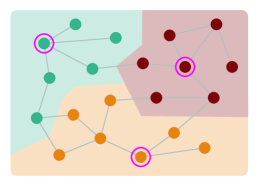
Figure 1: Voronoi diagram on a graph. Nodes with circles represent the current sensor positions. Each colored area represents the Voronoi region corresponding to each sensor.

$$\mathcal{W}_{i,t}=\{v\in\mathcal{V}|d(v,q_{i,t})<d(v,q_{j,t}),\forall q_{j}\in\mathcal{Q}_{t}\},$$ (23)

where $d(v,q_{i})$ is the shortest distance between $v$ and $q_{i}$ and $\mathcal{Q}_{t}=\{q_{j,t}\}_{j=1,\ldots,K}$ denotes the set of all sensor positions at $t$. Note that, in each $\mathcal{W}_{i,t}$, only one sensor is contained: We illustrate its example in Fig. 1. By utilizing (23), we can rewrite (22) for seeking the best position of a sensor within its Voronoi region $\mathcal{W}_{i,t}$ as follows.

$$q^{*}_{i,t+1}=\mathop{\rm arg~{}max}\limits_{y\in\mathcal{W}_{i,t}}\|\bm{\nu}_{y}\|^{2}-\|\mathbf{P}_{\mathcal{R}(\mathbf{N}_{:\mathcal{M}_{i,t}})}\bm{\nu}_{y}\|^{2}.$$ (24)

Since (24) depends only on its Voronoi region, all sensor selections in (24) are independent of each other. Therefore, we can select sensors by (24) in a distributed fashion. It allows for saving the communication cost of each sensor as well as the optimization cost.

When we assume mobile sensors, their movable areas could be restricted to their neighbors. To reflect this, we can further impose a constraint on the Voronoi region where the movable nodes are restricted to the $P$-hop neighbors of the target node. The $P$-hop neighbor of the $i$th sensor (node) is defined as

$$\mathcal{N}_{i,t}^{P}=\{v\in\mathcal{V}|d(v,q_{i,t})\leq P\}.$$ (25)

As a result, the proposed control law of sensors in (24) is further modified as follows:

$$q^{*}_{i,t+1}=\mathop{\rm arg~{}max}\limits_{y\in\mathcal{W}_{i,t}\cap\mathcal{N}_{i,t}^{P}}\|\bm{\nu}_{y}\|^{2}-\|\mathbf{P}_{\mathcal{R}(\mathbf{N}_{:\mathcal{M}_{i,t}})}\bm{\nu}_{y}\|^{2}.$$ (26)

Algorithm 2 summarizes the proposed dynamic sensor placement method.

Input: Sensing matrix $\mathbf{G}$, initial positions of sensors $\mathcal{Q}_{1}$, time duration $T$

for $t=1,\ldots,T$ do

       Update the data matrix $\mathbf{X}_{t}$

       Calculate the Voronoi regions $\{\mathcal{W}_{i,t}\}_{i=1,\ldots,K}$

       Calculate the $P$ hop neighbors $\{\mathcal{N}^{P}_{i,t}\}_{i=1,\ldots,K}$

       Update the dictionary $\mathbf{A}_{t}$ with Algorithm 1

       $\mathbf{N}_{t}\leftarrow\mathbf{A}^{\top}_{t}\mathbf{G}$

       Calculate $\mathbf{P}_{\mathcal{R}(\mathbf{N}_{:\mathcal{M}_{i,t}})}$

       par for $i=1,\ldots,K$ 

             $q^{*}_{i,t+1}=\mathop{\rm arg~{}max}\limits_{y\in\mathcal{W}_{i,t}\cap\mathcal{N}_{i,t}^{P}}\|\bm{\nu}_{y}\|^{2}-\|\mathbf{P}_{\mathcal{R}(\mathbf{N}_{:\mathcal{M}_{i,t}})}\bm{\nu}_{y}\|^{2}$

            

      $\mathcal{Q}_{t+1}\leftarrow\{q^{*}_{i,t+1}\}_{i=1,\ldots,K}$

      

Output: Sensor positions $\{\mathcal{Q}_{t}\}_{t=1,\ldots,T+1}$

Algorithm 2 Dynamic Sensor placement

4 EXPERIMENTS

In this section, we compare reconstruction errors of time-varying graph signals measured by selected positions of sensors. We perform recovery experiments for synthetic and real datasets.

4.1 SYNTHETIC GRAPH SIGNALS

In this subsection, we perform dynamic sensor placement for synthetic data.

4.1.1 SETUP

In the synthetic case, the recovery experiment is performed for signals on a random sensor graph with $N=256$. The number of sensors is set to $K=8$. We consider the following graph signals:

Bandlimited (BL) model

The BL model is defined in (3). We set to $B=N/16$. We generate expansion coefficients $\mathbf{d}_{t}$ as follows:

$$\mathbf{d}_{t}=\begin{bmatrix}\frac{1}{t}\times\sin(10t+\phi_{i})+1\\ \vdots\\ \frac{1}{t}\times\sin(10t+\phi_{K})+1\end{bmatrix},$$ (27)

where $\phi_{i}=\frac{\pi}{K}i$. In this model, graph signals temporally oscillate with the fixed bandwidth, and their oscillation amplitudes decay. It would mimic a possible physical data observation model, e.g., temperature and humidity.

Piecewise-constant (PC) model

The PC model is defined in (4). The number of clusters is set to $C=3$. We randomly separate nodes into $C$ clusters so that nodes in a cluster are connected. We generate $\mathbf{d}_{t}$ as follows:

$$\mathbf{d}_{t}=\begin{bmatrix}\frac{1}{t}\times\sin(6t+\frac{2\pi}{3})+1\\ \frac{1}{t}\times 2\sin(8t+\frac{4\pi}{3})+1\\ \frac{1}{t}\times 3\sin(10t)+1\end{bmatrix}.$$ (28)

In this model, signal values in a cluster change simultaneously (but the temporal frequencies are different for different clusters). It can be a possible model for datasets of physically distinct environments, e.g., warehouses, where signal values within the communities are more correlated than those between clusters.

For both graph signal models, we generate the data matrix $\mathbf{X}$ with $T=40$. The number of time slots is set to $D=20$. We set the temporal sampling period $T_{s}=\frac{\pi}{30}$ to avoid aliasing. The parameters of the dictionary learning are set to $(\mu,\gamma)=(2,0.5)$ and $P=2$ is used for the sensor movable area.

Recovery accuracy is measured both for noiseless (clean) and noisy cases. For the noisy case, white Gaussian noise $w[i]\sim\mathcal{N}(0,0.25)$ is added to the signals. We compare the signal reconstruction accuracy of the proposed method with those of the following existing methods.

1. SVD1: Fixed sensor placement [22] whose dictionary is learned by SVD once at $t=0$.

2. SVD2: Fixed sensor placement similar to SVD1 but whose dictionary is sequentially learned by the SVD at every time instance.

For all methods, the initial position of sensors is randomly chosen. We calculate the averaged MSEs for 50 independent runs.

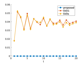
(a) BL model

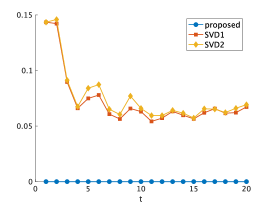
(b) PC model

Figure 2: MSE comparison of the reconstructed synthetic data for the noiseless case.

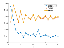
(a) BL model

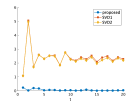
(b) PC model

Figure 3: MSE comparison of the reconstructed synthetic data for the noisy case.

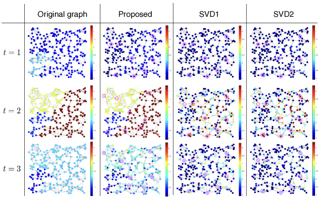
Figure 4: Reconstructed graph signals for PC signals at time $t=1,2,3$. Circled nodes represent selected sensor positions.

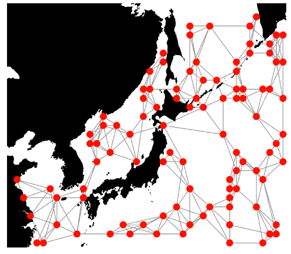
Figure 5: 5-nearest neighbor graph for sea surface temperature data.

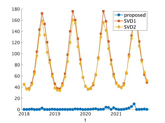
Figure 6: Comparison of reconstruction MSEs of sea surface temperature data.

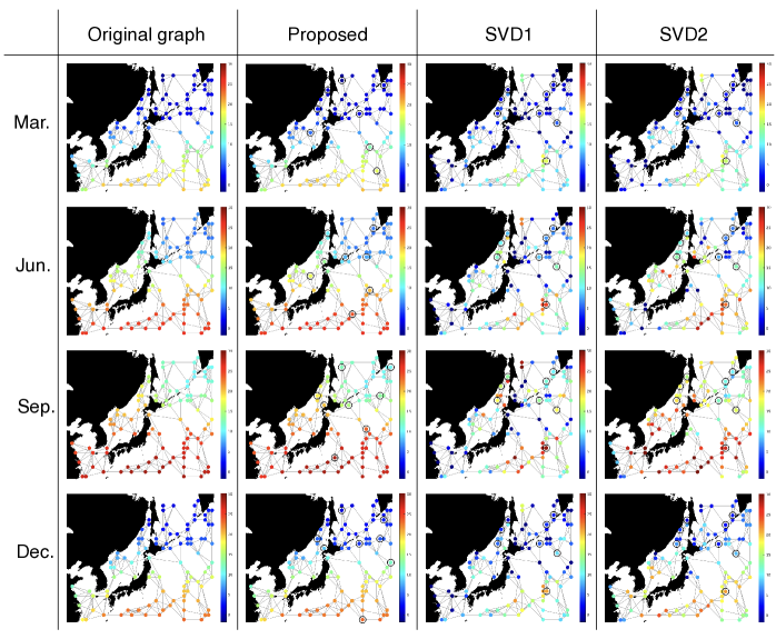
Figure 7: Reconstructed graph signals of sea surface temperature data. Circled nodes represent sensor positions.

4.1.2 RESULTS

Figs. 2 and 3 show the experimental results for the noiseless and noisy cases, respectively. We also show examples of the original and reconstructed graph signals of PC models for the noisy case in Fig. 4. Due to space limitation, we only show reconstructed graph signals for $t=1,2,3$ in Fig. 4. From Figs. 2 and 3, the proposed method show consistently (and significantly) smaller MSEs than other methods in all-time instances for both noiseless and noisy cases. For the noiseless case, the proposed method achieves perfect recovery thanks to graph sampling theory. For the noisy case, the MSE of the proposed method gradually decreases over time. This indicates that the proposed method can adapt to the change in measurement conditions, while the static methods fail to do so.

4.2 REAL-WORLD DATASET

In this subsection, we perform dynamic sensor placement for real data to validate the proposed method for practical observations.

4.2.1 SETUP

We use the global sea surface temperature data set during 2017-2021. It is publicly available online [43]. This dataset is composed of snapshots recorded every month from 2017 to 2021, i.e., its duration is $T=60$. Temperature is sampled at intersections of 1-degree latitude-longitude grids. For simplicity, we clip snapshots around Japan and randomly sample 100 nodes for the experiments. Then, we construct a $5$-nearest neighbor graph. We remove the edges across the mainland Japan. The obtained graph is shown in Fig. 5. The number of time slots and sensors are set to $D=12,K=8$. Similar to the previous section, we reconstruct the graph signals from the observations at the selected sensor locations. We evaluate the averaged MSEs for 30 independent runs and compare it with the above-mentioned two methods.

4.2.2 RESULTS

Fig. 6 shows the MSEs. As with the experiment for the synthetic data, the proposed dynamic sensor placement presents significantly lower MSEs than the SVD-based methods. SVD2 exhibits slightly lower MSEs than SVD1 because SVD2 can update the dictionary at all time instances, while SVD1 uses the static dictionary.

A part of the original and reconstructed graph signals are visualized in Fig. 7. The proposed methods place many sensors in the northern area in March and December (cold season), while the positions are more uniformly distributed in June and September (warm season). This could reflect that the sea temperature in the northern area drastically drops in the cold season as shown in Fig.7. Therefore, sensors move to north to capture such a temperature change. Fig. 7 also demonstrates that the signal recovery performance of the proposed method is better than the existing methods.

5 CONCLUSION

In this paper, we propose a dynamic sensor placement method based on graph sampling theory. We sequentially learn the dictionary from a time series of observed graph signals by utilizing sparse coding. Using the dictionary, we dynamically determine the sensor placement in every time instance such that the non-observed graph signal can be best recovered. In experiments, we demonstrate that the proposed method outperforms existing static sensor placement methods in synthetic and real datasets.

References

- [1] S. Tilak, N. B. Abu-Ghazaleh, and W. Heinzelman, “Infrastructure tradeoffs for sensor networks,” in Proceedings of the 1st ACM international workshop on Wireless sensor networks and applications, 2002, pp. 49–58.
- [2] L. M. Oliveira and J. J. Rodrigues, “Wireless Sensor Networks: A Survey on Environmental Monitoring.” J. Commun., vol. 6, no. 2, pp. 143–151, 2011.
- [3] T.-H. Yi and H.-N. Li, “Methodology developments in sensor placement for health monitoring of civil infrastructures,” International Journal of Distributed Sensor Networks, vol. 8, no. 8, p. 612726, 2012, publisher: SAGE Publications Sage UK: London, England.
- [4] K. Visalini, B. Subathra, S. Srinivasan, G. Palmieri, K. Bekiroglu, and S. Thiyaku, “Sensor Placement Algorithm With Range Constraints for Precision Agriculture,” IEEE Aerospace and Electronic Systems Magazine, vol. 34, no. 6, pp. 4–15, Jun. 2019, conference Name: IEEE Aerospace and Electronic Systems Magazine.
- [5] Z. Wang, H.-X. Li, and C. Chen, “Reinforcement learning-based optimal sensor placement for spatiotemporal modeling,” IEEE Trans. Cybern., vol. 50, no. 6, pp. 2861–2871, 2019, publisher: IEEE.
- [6] K. Manohar, B. W. Brunton, J. N. Kutz, and S. L. Brunton, “Data-driven sparse sensor placement for reconstruction: Demonstrating the benefits of exploiting known patterns,” IEEE Contr. Syst. Mag., vol. 38, no. 3, pp. 63–86, 2018, publisher: IEEE.
- [7] F. Y. Lin and P.-L. Chiu, “A near-optimal sensor placement algorithm to achieve complete coverage-discrimination in sensor networks,” IEEE Commun. Lett., vol. 9, no. 1, pp. 43–45, 2005, publisher: IEEE.
- [8] A. Sakiyama, Y. Tanaka, T. Tanaka, and A. Ortega, “Efficient sensor position selection using graph signal sampling theory,” in 2016 IEEE International Conference on Acoustics, Speech and Signal Processing (ICASSP), Mar. 2016, pp. 6225–6229.
- [9] ——, “Eigendecomposition-free sampling set selection for graph signals,” IEEE Trans. Signal Process., vol. 67, no. 10, pp. 2679–2692, May 2019.
- [10] Y. Jiang, J. Bigot, and S. Maabout, “Sensor selection on graphs via data-driven node sub-sampling in network time series,” arXiv:2004.11815 [cs, stat], Apr. 2020, arXiv: 2004.11815. [Online]. Available: http://arxiv.org/abs/2004.11815
- [11] A. Downey, C. Hu, and S. Laflamme, “Optimal sensor placement within a hybrid dense sensor network using an adaptive genetic algorithm with learning gene pool,” Structural Health Monitoring, vol. 17, no. 3, pp. 450–460, 2018, publisher: SAGE Publications Sage UK: London, England.
- [12] J. Li, “Exploring the potential of utilizing unsupervised machine learning for urban drainage sensor placement under future rainfall uncertainty,” Journal of Environmental Management, vol. 296, p. 113191, 2021, publisher: Elsevier.
- [13] S. Joshi and S. Boyd, “Sensor selection via convex optimization,” IEEE Trans. Signal Process., vol. 57, no. 2, pp. 451–462, 2008, publisher: IEEE.
- [14] ——, “Sensor Selection via Convex Optimization,” IEEE Trans. Signal Process., vol. 57, no. 2, pp. 451–462, Feb. 2009. [Online]. Available: http://ieeexplore.ieee.org/document/4663892/
- [15] T. Nagata, T. Nonomura, K. Nakai, K. Yamada, Y. Saito, and S. Ono, “Data-Driven Sparse Sensor Selection Based on A-Optimal Design of Experiment With ADMM,” IEEE Sensors Journal, vol. 21, no. 13, pp. 15 248–15 257, Jul. 2021, conference Name: IEEE Sensors Journal.
- [16] A. Krause, A. Singh, and C. Guestrin, “Near-Optimal Sensor Placements in Gaussian Processes: Theory, Efficient Algorithms and Empirical Studies,” J. Mach. Learn. Res., vol. 9, pp. 235–284, Jun. 2008.
- [17] E. Clark, T. Askham, S. L. Brunton, and J. Nathan Kutz, “Greedy Sensor Placement With Cost Constraints,” IEEE Sensors Journal, vol. 19, no. 7, pp. 2642–2656, Apr. 2019, conference Name: IEEE Sensors Journal.
- [18] C. Jiang, Y. C. Soh, and H. Li, “Sensor placement by maximal projection on minimum eigenspace for linear inverse problems,” IEEE Trans. Signal Process., vol. 64, no. 21, pp. 5595–5610, Nov. 2016.
- [19] E. J. Candès and M. B. Wakin, “An introduction to compressive sampling,” IEEE Signal Process. Mag., vol. 25, no. 2, pp. 21–30, 2008, publisher: IEEE.
- [20] R. G. Baraniuk, “Compressive sensing [lecture notes],” IEEE Signal Process. Mag., vol. 24, no. 4, pp. 118–121, 2007, publisher: IEEE.
- [21] Y. C. Eldar and G. Kutyniok, Compressed Sensing: Theory and Applications. Cambridge University Press, May 2012.
- [22] B. Jayaraman and S. M. Mamun, “On data-driven sparse sensing and linear estimation of fluid flows,” Sensors, vol. 20, no. 13, p. 3752, 2020, publisher: Multidisciplinary Digital Publishing Institute.
- [23] B. Li, H. Liu, and R. Wang, “Efficient Sensor Placement for Signal Reconstruction Based on Recursive Methods,” IEEE Trans. Signal Process., vol. 69, pp. 1885–1898, 2021, conference Name: IEEE Transactions on Signal Processing.
- [24] H. Zhou, X. Li, C.-Y. Cher, E. Kursun, H. Qian, and S.-C. Yao, “An information-theoretic framework for optimal temperature sensor allocation and full-chip thermal monitoring,” in DAC Design Automation Conference 2012. IEEE, 2012, pp. 642–647.
- [25] A. A. Alonso, C. E. Frouzakis, and I. G. Kevrekidis, “Optimal sensor placement for state reconstruction of distributed process systems,” AIChE Journal, vol. 50, no. 7, pp. 1438–1452, 2004, publisher: Wiley Online Library.
- [26] J. Hara and Y. Tanaka, “Sampling Set Selection for Graph Signals under Arbitrary Signal Priors,” in ICASSP 2022 - 2022 IEEE Int. Conf. Acoust. Speech Signal Process. (ICASSP), May 2022, pp. 5732–5736, iSSN: 2379-190X.
- [27] Y. Tanaka, Y. C. Eldar, A. Ortega, and G. Cheung, “Sampling signals on Graphs: From Theory to Applications,” IEEE Signal Process. Mag., vol. 37, no. 6, pp. 14–30, Nov. 2020.
- [28] S. Chen, R. Varma, A. Sandryhaila, and J. Kovačević, “Discrete signal processing on graphs: sampling theory,” IEEE Trans. Signal Process., vol. 63, no. 24, pp. 6510–6523, Dec. 2015.
- [29] A. Anis, A. Gadde, and A. Ortega, “Efficient Sampling Set Selection for Bandlimited Graph Signals Using Graph Spectral Proxies,” IEEE Trans. Signal Process., vol. 64, no. 14, pp. 3775–3789, Jul. 2016.
- [30] M. Tsitsvero, S. Barbarossa, and P. D. Lorenzo, “Signals on graphs: Uncertainty principle and sampling,” IEEE Trans. Signal Process., vol. 64, no. 18, pp. 4845–4860, Sep. 2016.
- [31] G. Puy, N. Tremblay, R. Gribonval, and P. Vandergheynst, “Random sampling of bandlimited signals on graphs,” Applied and Computational Harmonic Analysis, vol. 44, no. 2, pp. 446–475, Mar. 2018.
- [32] X. Wang, J. Chen, and Y. Gu, “Local measurement and reconstruction for noisy bandlimited graph signals,” Signal Processing, vol. 129, pp. 119–129, Dec. 2016. [Online]. Available: https://www.sciencedirect.com/science/article/pii/S0165168416301001
- [33] S. Chen, R. Varma, A. Singh, and J. Kovacevic, “Representations of piecewise smooth signals on graphs,” in 2016 IEEE Int. Conf. Acoust. Speech Signal Process. (ICASSP). IEEE, Mar. 2016, pp. 6370–6374.
- [34] Y. C. Eldar, Sampling Theory: Beyond Bandlimited Systems. Cambridge University Press, Apr. 2015.
- [35] Y. Tanaka and Y. C. Eldar, “Generalized sampling on graphs with subspace and smoothness priors,” IEEE Trans. Signal Process., vol. 68, pp. 2272–2286, 2020.
- [36] J. Hara, Y. Tanaka, and Y. C. Eldar, “Graph Signal Sampling Under Stochastic Priors,” Jun. 2022, arXiv:2206.00382 [eess].
- [37] D. I. Shuman, B. Ricaud, and P. Vandergheynst, “Vertex-Frequency Analysis on Graphs.”
- [38] L. Condat, “A Primal–Dual Splitting Method for Convex Optimization Involving Lipschitzian, Proximable and Linear Composite Terms,” J Optim Theory Appl, vol. 158, no. 2, pp. 460–479, Aug. 2013. [Online]. Available: http://link.springer.com/10.1007/s10957-012-0245-9
- [39] F. Zhang, The Schur Complement and Its Applications. Springer Science & Business Media, Mar. 2006.
- [40] G. B. Passty, “Ergodic convergence to a zero of the sum of monotone operators in Hilbert space,” Journal of Mathematical Analysis and Applications, vol. 72, no. 2, pp. 383–390, 1979, publisher: Elsevier.
- [41] P. Tseng, “Applications of a splitting algorithm to decomposition in convex programming and variational inequalities,” SIAM Journal on Control and Optimization, vol. 29, no. 1, pp. 119–138, 1991, publisher: SIAM.
- [42] P. L. Combettes and V. R. Wajs, “Signal recovery by proximal forward-backward splitting,” Multiscale modeling & simulation, vol. 4, no. 4, pp. 1168–1200, 2005, publisher: SIAM.
- [43] N. A. A. Rayner, D. E. Parker, E. B. Horton, C. K. Folland, L. V. Alexander, D. P. Rowell, E. C. Kent, and A. Kaplan, “Global analyses of sea surface temperature, sea ice, and night marine air temperature since the late nineteenth century,” Journal of Geophysical Research: Atmospheres, vol. 108, no. D14, 2003, publisher: Wiley Online Library.