A Multivariate Functional-Data Mixture Model for Spatio-Temporal Data: Inference and Cokriging

Abstract

In this paper, we introduce a model for multivariate, spatio-temporal functional data. Specifically, this work proposes a mixture model that is used to perform spatio-temporal prediction (cokriging) when both the response and the additional covariates are functional data. The estimation of such models in the context of expansive data poses many methodological and computational challenges. We propose a new Monte Carlo Expectation Maximization algorithm based on importance sampling to estimate model parameters. We validate our methodology using simulation studies and provide a comparison to previously proposed functional clustering methodologies. To tackle computational challenges, we describe a variety of advances that enable application on large spatio-temporal datasets.

The methodology is applied on Argo oceanographic data in the Southern Ocean to predict oxygen concentration, which is critical to ocean biodiversity and reflects fundamental aspects of the carbon cycle. Our model and implementation comprehensively provide oxygen predictions and their estimated uncertainty as well as recover established oceanographic fronts.

Keywords: functional regression, clustering, penalized splines, physical and biogeochemical oceanography

1 Introduction

The rapid growth of high-resolution and multivariate data motivates continued advances in flexible and efficient statistical methodology. One prime example is the Argo data, which is collected by floats that measure temperature and salinity at different depths in the ocean (see Figure 1 and Argo,, 2020). An important expansion of the Argo Project’s goals is Biogeochemical (BGC) Argo, which has added a limited number of floats that also measure oxygen and nitrate, among other variables (Claustre et al.,, 2020). Biogeochemical floats require additional sensors leading to higher fixed and maintenance costs than Core Argo floats (Bittig et al.,, 2019). Thus, it is not practical to introduce the same coverage as achieved by Core Argo floats; in the Southern Ocean during 2020, Core Argo floats collected approximately 12,000 profiles (each being a collection of temperature and salinity measurements at varying depths for one location) while BGC Argo floats collected just 2,600 over the same time period (see Figure 1).

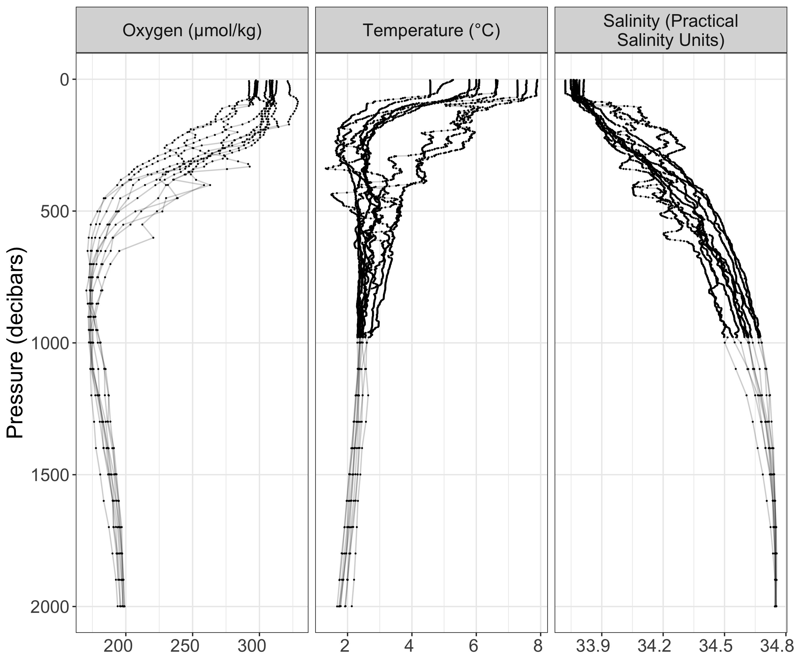
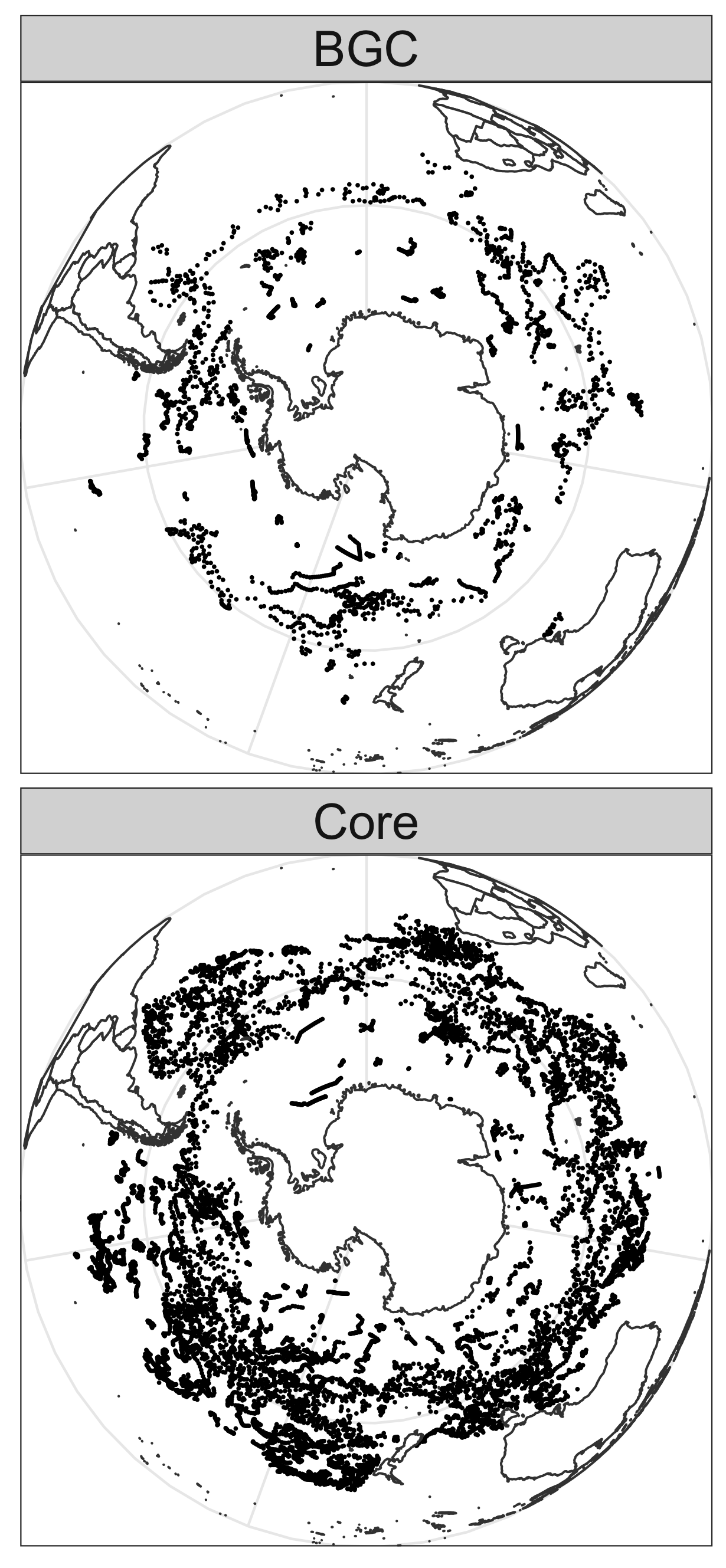
Figure 1: (Left) Oxygen, temperature, and salinity data of ten profiles collected from a BGC Argo float (WMO #5904679) as a function of pressure (1 decibar of pressure is approximately 1 meter of depth). (Top Right) Locations of BGC profiles collected in the Southern Ocean in 2020 by the Southern Ocean Carbon and Climate Observations and Modeling (SOCCOM) Project and (Bottom Right) locations of nearby Core Argo profiles collected in 2020.

However, biogeochemical information plays a vital role in the understanding of the world’s carbon cycle as well as ocean ecosystems (Claustre et al.,, 2020). Consequently, the imbalance between Core Argo and BGC Argo floats calls for statistical methodology exploiting correlation of biogeochemical data with temperature and salinity to reconstruct biogeochemical data for Core Argo floats. One approach that has been employed by oceanographers is to fit a random forest, which represents well the complex relationships between the variables (Giglio et al.,, 2018). However, their analysis is restricted to one fixed depth at a time and consequently cannot model correlation between measurements stemming from the same profile. Instead, we view the Argo profiles as functional data indexed by space and time (Yarger et al.,, 2022). This approach leverages the correlation in depth and provides principled prediction of entire functions, dimension reduction through functional principal components analysis for efficient computation, and a concrete model for the covariance structure of the data.

One major challenge of modeling oceanographic data in the Southern Ocean is that the transition from warmer subtropical waters in the north to colder Antarctic waters does not occur smoothly. Instead, ocean properties are characterized by a series of sudden changes, occurring at so-called fronts — sharp transition zones generally aligned east–west (Chapman et al.,, 2020; Orsi et al.,, 1995). Consequently, any stationarity assumption on the data across different fronts will be violated. However, it is established that water properties between fronts tend to be homogeneous (Chapman et al.,, 2020). To handle the sudden changes in the distribution of the data caused by fronts while simultaneously exploiting the homogeneity of water properties between fronts, we propose a functional spatio-temporal regression mixture model.

Our work builds upon a strong foundation of research in functional data analysis and spatial statistics. To start, function-on-function regression has been comprehensively researched. We mention the seminal paper Yao et al., (2005) as well as Zhou et al., (2008) who formulate a likelihood-based estimation strategy for paired functional data. Modeling and estimation for spatially-correlated univariate functional data was studied in Zhou et al., (2010) and more recently in Zhang and Li, (2021) who also considered piece-wise stationary functional data to accommodate spatial discontinuities in housing prices due to neighborhood characteristics.

Spatial/spatio-temporal functional data that exhibit sudden changes are common, and substantial work has gone towards developing appropriate models. For example, Zheng and Serban, (2018) investigate geographic disparities in pediatric health, Margaritella et al., (2021) model regions of brain activity, and Frévent et al., (2021) cluster abnormal unemployment rates. Recently, Liang et al., (2020) proposed a clustering methodology for univariate data allowing for cluster-dependent covariance structures. In a finite dimensional setting, Bolin et al., (2019) developed latent Gaussian random field mixture models for data observed on a regular grid, but the extension to a functional setting is not straightforward. In the oceanographic literature, approaches for identifying fronts include statistical modeling, though most use Gaussian mixture models that ignore spatial information (Thomas et al.,, 2021; Chapman et al.,, 2020).

We describe next our contributions and how the paper is organized. In Section 2, we propose a novel mixture model for multivariate, functional data with spatial dependence. We model the relationships between a univariate functional response and an arbitrary number of functional covariates. Furthermore, our approach can effectively handle irregularly-sampled data in both the spatial and functional dimensions of the data.

In Section 3, we discuss parameter estimation, prediction, and model selection. We introduce a Monte Carlo Expectation Maximization (MCEM) algorithm (Wei and Tanner,, 1990) using importance sampling, which improves upon strategies employed in previous works (cf. Liang et al.,, 2020). In Section 3.3, we discuss how the estimated model can be used for predicting the response with available predictor data, while addressing the uncertainty of prediction based on that of the cluster memberships. Thus far, functional kriging and cokriging in the context of functional mixture models have not been studied. Furthermore, we provide a tractable AIC criterion in the presence of latent variables for model selection. In Section 4, we show in simulation studies that our EM algorithm produces viable parameter estimates and clustering results. In Section 5, we describe our analysis on the Argo data, which shows that the model provides quality predictions of biogeochemical variables with sensible uncertainty quantification. Furthermore, we recover established oceanographic fronts as a part of the clustering procedure. Finally, we discuss the outlook and potential improvements to our work in Section 6.

The Argo data considered here consists of more than ten thousand locations and millions of observations. Consequently, reducing the runtime and memory usage of the model estimation and prediction procedure is essential. This work is accompanied by an R package implementing our methodology where crucial parts of the estimation and prediction procedure are written in C++, available at https://github.com/dyarger/argo_clustering_cokriging. Our software seamlessly integrates a Vecchia approximation of the likelihood when modeling spatial dependence (Guinness,, 2021). Furthermore, we exploit computational advantages of sparse matrices by circumventing the use of orthogonalized B-splines, an approach widely used in the functional data literature.

2 Model and Assumptions

In this section we provide the framework for our modeling. Let $\mathcal{S}$ and $\mathcal{T}$ be two index sets. The set $\mathcal{S}$ may correspond to a spatial index and the set $\mathcal{T}$ a temporal index, but this is not necessary. In our motivating application, $\mathcal{S}$ will correspond to a spatio-temporal index, and $\mathcal{T}$ will correspond to ocean depths. For a location $s_{i}\in\mathcal{S}$, where $i=1,2,\dots,n$, we observe measurements for a response $Y$ and covariates $X_{1},\dots,X_{K}$:

$$\{Y(s_{i},t_{ij}):(s_{i},t_{ij})\in\mathcal{S}\times\mathcal{T}\}_{j=1}^{n_{i}}, \{X_{k}(s_{i},t_{ij}):(s_{i},t_{ij})\in\mathcal{S}\times\mathcal{T}\}_{j=1}^{n_{i}},~{}~{}k=1,\dots,K.$$

The indices $t_{ij}$ and the number of observations $n_{i}$ may vary for different locations $s_{i}$ and across the covariates and the response. Our implementation reflects this, but for notational simplicity we omit their dependence on $s_{i}$, $X_{k}$, or $Y$. In our application, the response $Y$ is a biogeochemical variable, while temperature and salinity are the covariates $X_{1}$ and $X_{2}$.

2.1 Mixed Functional Spatio-temporal Linear Regression

We model sudden changes in the spatio-temporal distribution via an unobserved latent field $\{Z(s_{i})\}_{i=1}^{n}$ where $Z(s_{i})$ takes values in $\{1,\dots,G\}$ for some $G$ to be identified. We will use the random field $\{Z(s)\}$ to partition the data into $G$ clusters and fit separate models for each cluster. To model spatio-temporal dependence, we assume that $\{Z_{i}:=Z(s_{i})\}_{i=1}^{n}$ forms a Markov random field (MRF), where the distribution of $Z_{i}$ conditional on its neighbors $\partial Z_{i}$ is the Gibbs distribution with parameter $\xi$, that is

$$\mathbb{P}(Z_{i}=g|\partial Z_{i},\xi)\propto\exp\left(\xi\sum_{z\in\partial Z_{i}}\mathbb{I}(z=g)\right).$$ (1)

This model was proposed in Jiang and Serban, (2012) and used in Liang et al., (2020). We use graphs defined by k-nearest-neighbors ignoring the direction of the edges to obtain a symmetric neighborhood structure.

The observations are modeled as samples from unknown continuous random functions, observed with additive measurement errors. Notationally, we use calligraphic letters to denote the underlying functions and regular letters for the observations. Specifically, let

$$Y(s_{i},t_{ij}) =\mathcal{Y}(s_{i},t_{ij})+\epsilon_{ij}^{Y}=\sum_{g=1}^{G}\mathbb{I}(Z_{i}=g)\,\mathcal{Y}_{g}(s_{i},t_{ij})+\epsilon_{ij}^{Y},$$

$$X_{k}(s_{i},t_{ij}) =\mathcal{X}_{k}(s_{i},t_{ij})+\epsilon_{ij}^{k}=\sum_{g=1}^{G}\mathbb{I}(Z_{i}=g)\,\mathcal{X}_{g,k}(s_{i},t_{ij})+\epsilon_{ij}^{k},~{}~{}k=1,\dots,K,$$

where $\mathcal{Y}_{g}=\{\mathcal{Y}_{g}(s,t)\}$ and $\mathcal{X}_{g,k}=\{\mathcal{X}_{g,k}(s,t)\}$ are latent stochastic processes governing the spatio-temporal dependence within each cluster $g$. The cluster memberships $Z_{i}$ are unobserved. We assume that the underlying functional processes $\mathcal{Y}_{g}$ and $\mathcal{X}_{g,k}$ for different clusters are independent in $g$. The measurement errors for each variable are modeled as i.i.d. mean-zero Gaussian random variables.

For each cluster $g$, the $\{\mathcal{Y}_{g}(s_{i},\cdot)\}$ and $\{\mathcal{X}_{g,k}(s_{i},\cdot)\}$ are modeled as stationary function-valued random fields taking values in the Hilbert spaces of functions $\mathbb{H}_{Y}$ and $\mathbb{H}_{k}$ respectively. For simplicity, we assume that $\mathbb{H}_{Y}=\mathbb{H}_{1}=\dots=\mathbb{H}_{K}=:\mathbb{H}$, and we choose $\mathbb{H}$ to be the space of square integrable functions on some compact interval $[a,b]$. We collect all of the covariates in a vector $\mathcal{X}_{g}(s_{i},\cdot):=(\mathcal{X}_{g,1}(s_{i},\cdot),\dots,\mathcal{X}_{g,K}(s_{i},\cdot))^{\top},$ such that $\{\mathcal{X}_{g}(s,\cdot):s\in\mathcal{S}\}$ is a random field taking values in $\mathbb{H}^{K}$, the direct sum of the Hilbert spaces. We endow $\mathbb{H}^{K}$ with the weighted inner product $\langle f,g\rangle_{\mathbb{H}^{K}}=\sum_{k=1}^{K}w_{k}\langle f_{k},g_{k}\rangle_{\mathbb{H}}$ (Happ and Greven,, 2018).

Finally, our spatio-temporal mixed regression model links the two latent processes via

$$\mathcal{Y}_{g}(s,t)=\mu_{g,\mathcal{Y}}(t)+\mathscr{F}_{g}(\mathcal{X}_{g}(s,\cdot)-\mu_{g,\mathcal{X}}(\cdot))(t)+\mathcal{E}_{g}(s,t).$$

Here, $\mu_{g,\mathcal{Y}}$ and $\mu_{g,\mathcal{X}}$ are the mean functions of the random fields $\{\mathcal{Y}_{g}(s,\cdot)\}$ and $\{\mathcal{X}_{g}(s,\cdot)\}$, respectively, $\mathscr{F}_{g}$ is a bounded linear operator from $\mathbb{H}^{K}$ to $\mathbb{H}$, and the $\{\mathcal{E}_{g}(s,\cdot):s\in\mathcal{S}\}$ form an $\mathbb{H}$-valued, stationary, zero-mean random field representing a correlated spatio-temporal random effect in cluster $g$, which is independent from the covariates $\mathcal{X}_{g,k}$. The linear operator $\mathscr{F}_{g}$ describes how the predictor processes relate to the response process, while $\mathcal{E}_{g}$ represents variability unexplained by $\mathcal{X}_{g}$.

2.2 Dimension Reduction With Principal Components

Directly modeling functions in infinite-dimensional spaces is infeasible, so suitable representation and dimension reduction is necessary. To this end, we use a Karhunen-Loève expansion (cf. Hsing and Eubank,, 2015) to write

$$\mathcal{X}_{g}(s,\cdot)=\mu_{\mathcal{X},g}(\cdot)+\sum_{\ell=1}^{\infty}\alpha_{g,\ell}(s)\psi_{g,\ell}(\cdot),~{}~{}~{}~{}\mathcal{E}_{g}(s,\cdot)=\sum_{\ell=1}^{\infty}\eta_{g,\ell}(s)\phi_{g,\ell}(\cdot),$$

where $\mu_{\mathcal{X},g}$ and $\psi_{g,\ell}$ take values in $\mathbb{R}^{K}$ and $\phi_{g,\ell}$ takes values in $\mathbb{R}$. The $\{\alpha_{g,\ell}(s)\}_{\ell=1}^{\infty}$ and $\{\eta_{g,\ell}(s)\}_{\ell=1}^{\infty}$ are principal component scores at $s$, and $\{\psi_{g,\ell}\}_{\ell=1}^{\infty}$ and $\{\phi_{g,\ell}\}_{\ell=1}^{\infty}$ are orthonormal principal component functions of $\mathcal{X}_{g}$ and $\mathcal{E}_{g}$ respectively. In practice, the infinite sums are approximated by using only a small number of leading principal components. If $Q_{1}$ and $Q_{2}$ denote the number of principal components for $\mathcal{X}_{g}$ and $\mathcal{E}_{g}$ respectively, our model becomes

$$\mathcal{Y}_{g}(s,t)=\mu_{g,\mathcal{Y}}(t)+\sum_{\ell=1}^{Q_{1}}\alpha_{g,\ell}(s)(\mathscr{F}_{g}\psi_{g,\ell})(t)+\sum_{\ell=1}^{Q_{2}}\eta_{g,\ell}(s)\phi_{g,\ell}(t).$$

2.3 Modeling Spatio-temporal Correlation

Following Yarger et al., (2022), we model the spatio-temporal correlation of the random functions via the spatio-temporal correlations of their principal component scores. More precisely, we assume that the $\{\alpha_{g,\ell}(s)\}$ are stationary, zero-mean, Gaussian random fields that are uncorrelated across $g$ and $\ell$. Similarly, we assume that $\{\eta_{g,\ell}(s)\}$ have the same structure and are independent of all $\{\alpha_{g,\ell}(s)\}$. While the stationarity assumption seems restrictive, it is only imposed within each cluster $g$, and the combined model accommodates heterogeneity. For a specific data application, it remains to choose a suitable (valid) family of covariance function for the Gaussian processes. A commonly-used family is the Matérn covariance (Stein,, 2013), which provides flexibility for the smoothness and range of spatial correlation in the process, written in closed form for parameters $\sigma^{2},\kappa,\nu>0$ as

$$C(s,s^{\prime}) =\frac{\sigma^{2}}{2^{\nu-1}\Gamma(\nu)}\left(\frac{\left\lVert s-s^{\prime}\right\rVert}{\kappa}\right)^{\nu}\mathcal{K}_{\nu}\left(\frac{\left\lVert s-s^{\prime}\right\rVert}{\kappa}\right),$$

where $\mathcal{K}_{\nu}$ is the modified Bessel function of the second kind with order $\nu$, and $\Gamma$ is the gamma function. Here and throughout, $\left\lVert\cdot\right\rVert$ denotes the Euclidean norm on the respective space. The parameters are allowed to vary for different principal components and clusters. We will describe the specific covariance functions we use in Sections 4 and 5.

3 Model Estimation

3.1 Function Approximation Using Polynomial Splines

To approximate the mean functions and the principal component functions, we use spline bases. For notational ease, we use the same spline basis for all functions, though this is not necessary. Let $\{b_{1},\dots,b_{P}\}$ denote the functions forming a $P$-dimensional cubic spline basis on the interval $[a,b]$. Let $B(t)\in\mathbb{R}^{1\times P}$ denote the row vector of spline evaluations $(b_{1}(t),\dots,b_{P}(t))$. Then we approximate $\mu_{g,\mathcal{Y}}(t)\approx B(t)\theta_{g,\mathcal{Y}}$ where $\theta_{g,\mathcal{Y}}$ is a $P$-dimensional vector of spline coefficients. For the multivariate functional covariates, we write

$$\mu_{g,\mathcal{X}}(t)\approx\left(I_{K}\otimes B(t)\right)\begin{pmatrix}\theta_{g,\mathcal{X},1}^{\top}&\cdots&\theta_{g,\mathcal{X},K}^{\top}\end{pmatrix}^{\top}=:\left(I_{K}\otimes B(t)\right)\theta_{g,\mathcal{X}},$$

where $\otimes$ is the standard Kronecker product and $I_{K}$ denotes the $K\times K$ identity matrix. Using similar notation, we have $\left(\psi_{g,1}(t),\dots,\psi_{g,Q_{1}}(t)\right)^{\top}\approx\left(I_{K}\otimes B(t)\right)\Theta_{g,\mathcal{X}}$ for the predictor principal component functions, $\left((\mathscr{F}_{g}\psi_{g,1})(t),\dots,(\mathscr{F}_{g}\psi_{g,Q_{1}})(t)\right)^{\top}\approx B(t)\Lambda_{g}$, and $\left(\phi_{g,1}(t),\dots,\phi_{g,Q_{2}}(t)\right)^{\top}\approx B(t)\Theta_{g,\mathcal{E}}$, where $\Theta_{g,\mathcal{X}}$, $\Theta_{g,\mathcal{E}}$, and $\Lambda_{g}$ are matrices of spline coefficients of dimensions $KP\times Q_{1},P\times Q_{2}$, and $P\times Q_{1}$. If $\boldsymbol{\alpha}_{i}^{g}=(\alpha_{g,1}(s_{i}),\dots,\alpha_{g,Q_{1}}(s_{i}))^{\top}$ and $\boldsymbol{\eta}_{i}^{g}=(\eta_{g,1}(s_{i}),\dots,\eta_{g,Q_{2}}(s_{i}))^{\top}$, the model for the data can be succinctly written as follows:

$$X(s_{i},t_{ij}) =\sum_{g=1}^{G}\mathbb{I}(Z_{i}=g)\left[(I_{K}\otimes B(t_{ij}))\theta_{g,\mathcal{X}}+(I_{K}\otimes B(t_{ij}))\Theta_{g,\mathcal{X}}\boldsymbol{\alpha}_{i}^{g}\right]+(\epsilon_{ij}^{1},\dots,\epsilon_{ij}^{K})^{\top},$$ (2)

$$Y(s_{i},t_{ij}) =\sum_{g=1}^{G}\mathbb{I}(Z_{i}=g)\left[B(t_{ij})\theta_{g,\mathcal{Y}}+B(t_{ij})\Lambda_{g}\boldsymbol{\alpha}_{i}^{g}+B(t_{ij})\Theta_{g,\mathcal{E}}\boldsymbol{\eta}_{i}^{g}\right]+\epsilon^{Y}_{ij}.$$ (3)

Since the principal component functions are orthonormal, we impose the following orthonormality constraints for each $g$:

$$\Theta_{g,\mathcal{X}}^{\top}\left(I_{K}\otimes\int B(t)^{\top}B(t)\,\mathrm{d}t\,\right)\Theta_{g,\mathcal{X}}=I_{Q_{1}},~{}~{}~{}~{}\Theta_{g,\mathcal{E}}^{\top}\int B(t)^{\top}B(t)\,\mathrm{d}t\,\Theta_{g,\mathcal{E}}=I_{Q_{2}}.$$ (4)

Remark 1.

A common approach to enforce the orthogonality constraints in (4) is to use an orthogonalized spline basis $\tilde{B}(t)\in\mathbb{R}^{1\times P}$ and then require $\Theta_{g,\mathcal{X}}^{\top}\Theta_{g,\mathcal{X}}=I_{Q_{1}}$ and $\Theta_{g,\mathcal{E}}^{\top}\Theta_{g,\mathcal{E}}=I_{Q_{2}}$; see Zhou et al., (2010) and Liang et al., (2020), among others. However, for datasets as large as the Argo data, this becomes impractical because the evaluation matrices $\tilde{B}(t)$ (at observed data points) for orthogonalized splines are less sparse compared to regular B-splines. We outline in Section S5 how regular B-splines can be used to obtain algebraically identical estimates with great computational gains.

Remark 2.

The model as defined in (2) and (3) is not identifiable as the eigenfunctions are unique only up to their signs. However, identifiability can be effectively enforced in estimation by requiring the first entries in each column of $\Theta_{g,\mathcal{X}}$ and $\Theta_{g,\mathcal{E}}$ to be positive, and ordering the eigenfunctions by the marginal variances of the principal component scores.

3.2 Monte Carlo EM Algorithm

We aim to fit the model parameters denoted $\Omega$ by penalized likelihood maximization. First, we introduce some notation. We let $\boldsymbol{Z}:=(Z_{1},\dots,Z_{n})^{\top}$ be the vector of cluster memberships, $\boldsymbol{Y}_{i}\in\mathbb{R}^{n_{i}}$ the response observations at $s_{i}$, and $\boldsymbol{X}_{i}\in\mathbb{R}^{Kn_{i}}$ the vector of covariate observations arranged by covariate. Then we let $\boldsymbol{Y}:=(\boldsymbol{Y}_{1}^{\top},\dots,\boldsymbol{Y}_{n}^{\top})^{\top}$ and $\boldsymbol{X}:=(\boldsymbol{X}_{1}^{\top},\dots,\boldsymbol{X}_{n}^{\top})^{\top}$ be vectors of length $\sum_{i=1}^{n}n_{i}$ and $K\sum_{i=1}^{n}n_{i}$, respectively. Define the random vector $\boldsymbol{\alpha}_{i}:=\sum_{g=1}^{G}\mathbb{I}(Z_{i}=g)\boldsymbol{\alpha}_{i}^{g}.$ Finally, we use $\boldsymbol{\alpha}^{g}:=(\boldsymbol{\alpha}_{1}^{g\top},\dots,\boldsymbol{\alpha}_{n}^{g\top})^{\top}\in\mathbb{R}^{nQ_{1}}$ and $\boldsymbol{\alpha}:=(\boldsymbol{\alpha}_{1}^{\top},\dots,\boldsymbol{\alpha}_{n}^{\top})^{\top}\in\mathbb{R}^{nQ_{1}}$ and define $\boldsymbol{\eta},\boldsymbol{\eta}^{g}$, and $\boldsymbol{\eta}_{i}$ similarly.

To estimate $\Omega$, we maximize the penalized log-likelihood of the observed data

$$\ell(\Omega,\boldsymbol{X},\boldsymbol{Y})-\mathscr{P}(\Omega)=\log\int L(\Omega,\boldsymbol{X},\boldsymbol{Y},\boldsymbol{\alpha},\boldsymbol{\eta},\boldsymbol{Z})\,\mathrm{d}\boldsymbol{\alpha}\mathrm{d}\boldsymbol{\eta}\mathrm{d}\boldsymbol{Z}-\mathscr{P}(\Omega),$$ (5)

where $\mathscr{P}(\Omega)$ denotes a roughness penalty and $L$ denotes the likelihood function. We use the integrated squared second derivatives of the respective functions, which motivates our use of cubic B-splines (see Theorem 6.6.9 of Hsing and Eubank,, 2015). For example, for the mean function for $\mathcal{Y}_{g}$ and a smoothing parameter $\lambda_{\theta_{\mathcal{Y}}}$ to be chosen, we use the penalty

$$\mathcalboondox{p}(\theta_{g,\mathcal{Y}})=\lambda_{\theta_{\mathcal{Y}}}\theta_{g,\mathcal{Y}}^{\top}\int B^{(2)}(t)^{\top}B^{(2)}(t)\,\mathrm{d}t~{}\theta_{g,\mathcal{Y}},~{}~{}~{}\lambda_{\theta_{\mathcal{Y}}}>0.$$

We use similar penalties for the principal component functions as well as for the functions $\{\mathscr{F}_{g}\psi_{g,\ell}\}$, and let $\mathscr{P}(\Omega)$ then denote the sum of the individual penalties.

As the random vectors $\boldsymbol{\alpha},\boldsymbol{\eta}$ and $\boldsymbol{Z}$ are unobserved and direct maximization of (5) is not feasible, we employ the EM algorithm and treat $\boldsymbol{\alpha},\boldsymbol{\eta}$ and $\boldsymbol{Z}$ as latent variables. Given the assumptions, the log-likelihood of the complete data can be written

$$\begin{split}\ell(\Omega,\boldsymbol{X},\boldsymbol{Y},\boldsymbol{\alpha},\boldsymbol{\eta},\boldsymbol{Z})&=\ell(\Omega,\boldsymbol{Z})+\ell(\Omega,\boldsymbol{\alpha}|\boldsymbol{Z})+\ell(\Omega,\boldsymbol{\eta}|\boldsymbol{Z})\\ &\ \ \ \ \ +\sum_{i=1}^{n}\left[\ell(\Omega,\boldsymbol{Y}_{i}|\boldsymbol{\alpha}_{i},\boldsymbol{\eta}_{i},Z_{i})\ +\ell(\Omega,\boldsymbol{X}_{i}|\boldsymbol{\alpha}_{i},Z_{i})\right].\end{split}$$ (6)

We use the pseudo-likelihood $\sum_{i}\log\left[\mathbb{P}(Z_{i}|\partial Z_{i},\xi)\right]$ to replace $\ell(\Omega,\boldsymbol{Z})$ (cf. Besag,, 1975) in the following. The EM algorithm (Dempster et al.,, 1977) consists of initializing the parameters to $\Omega^{(1)}$ and alternating between the following two steps for $m=1,2,\dots$ until convergence:

1. E-step: Compute $\mathcal{Q}\left(\Omega|\Omega^{(m)}\right)=\mathbb{E}\left[\ell\left(\Omega,\boldsymbol{X},\boldsymbol{Y},\boldsymbol{\alpha},\boldsymbol{\eta},\boldsymbol{Z}\right)\middle|\boldsymbol{X},\boldsymbol{Y},\Omega^{(m)}\right]-\mathscr{P}(\Omega)$.

2. M-step: Update the parameters via $\Omega^{(m+1)}=\operatorname*{arg\,max}_{\Omega}\mathcal{Q}\left(\Omega|\Omega^{(m)}\right)$.

To compute $\mathcal{Q}\left(\Omega|\Omega^{(m)}\right)$ for the E-step, using the law of total expectation, we have

$$\mathbb{E} \left[\ell\left(\Omega,\boldsymbol{X},\boldsymbol{Y},\boldsymbol{\alpha},\boldsymbol{\eta},\boldsymbol{Z}\right)\middle|\boldsymbol{X},\boldsymbol{Y},\Omega^{(m)}\right]$$

$$=\sum_{z\in\mathcal{Z}}\mathbb{E}\left[\ell\left(\Omega,\boldsymbol{X},\boldsymbol{Y},\boldsymbol{\alpha},\boldsymbol{\eta},\boldsymbol{Z}\right)\middle|\boldsymbol{Z}=\boldsymbol{z},\boldsymbol{X},\boldsymbol{Y},\Omega^{(m)}\right]\mathbb{P}\left(\boldsymbol{Z}=\boldsymbol{z}|\boldsymbol{X},\boldsymbol{Y},\Omega^{(m)}\right),$$

where $\mathcal{Z}$ denotes the set of all possible configurations of $\boldsymbol{Z}$ values. Consequently, this is a sum over $G^{n}$ terms which, even for small $n$, is computationally intractable since the likelihood of the complete data does not factor due to spatial correlation. Thus, we use a Monte Carlo EM algorithm (Wei and Tanner,, 1990) as outlined next.

Monte Carlo E-Step. We propose to use importance sampling to estimate the expectation in $\mathcal{Q}\left(\Omega|\Omega^{(m)}\right)$. That is, we fix $T\in\mathbb{N}$ and create samples $\boldsymbol{\alpha}^{(\tau)},\boldsymbol{\eta}^{(\tau)},\boldsymbol{Z}^{(\tau)}$ for $\tau=1,\dots,T$ from a proposal distribution $h$ and approximate $\mathcal{Q}\left(\Omega|\Omega^{(m)}\right)$ via

$$\hat{\mathcal{Q}}\left(\Omega\middle|\Omega^{(m)}\right)=\left(\sum_{\tau=1}^{T}w^{(\tau)}\right)^{-1}\sum_{\tau=1}^{T}w^{(\tau)}\ell\left(\Omega,\boldsymbol{X},\boldsymbol{Y},\boldsymbol{\alpha}^{(\tau)},\boldsymbol{\eta}^{(\tau)},\boldsymbol{Z}^{(\tau)}\right)-\mathscr{P}(\Omega),$$ (7)

where the quantities $w^{(\tau)}=f(\boldsymbol{\alpha}^{(\tau)},\boldsymbol{\eta}^{(\tau)},\boldsymbol{Z}^{(\tau)}|\boldsymbol{X},\boldsymbol{Y},\Omega^{(m)})/h(\boldsymbol{\alpha}^{(\tau)},\boldsymbol{\eta}^{(\tau)},\boldsymbol{Z}^{(\tau)}|\Omega^{(m)})$ are called the importance sampling weights. To simplify the notation, we will drop the dependence on $\Omega^{(m)}$ below. For detailed information on importance sampling, see Robert and Casella, (2004). Our goal is to construct an $h$ that is easy to sample from and that is close to $f(\boldsymbol{\alpha}^{(\tau)},\boldsymbol{\eta}^{(\tau)},\boldsymbol{Z}^{(\tau)}|\boldsymbol{X},\boldsymbol{Y})$. First, note that for a given sample $\boldsymbol{Z}^{(\tau)}$, sampling from $f(\boldsymbol{\alpha},\boldsymbol{\eta}|\boldsymbol{Z}^{(\tau)},\boldsymbol{X},\boldsymbol{Y})$ is tractable; see Proposition 1 in the supplement S1. It remains to find a proposal denoted $\mathbb{P}_{I}$ for sampling $\boldsymbol{Z}^{(\tau)}|\boldsymbol{X},\boldsymbol{Y}$ and employ the following procedure:

1. Sample $\boldsymbol{Z}^{(\tau)}$ from $\mathbb{P}_{I}$ and compute $w^{(\tau)}$.

2. Sample $\boldsymbol{\alpha}^{(\tau)},\boldsymbol{\eta}^{(\tau)}$ from $f\left(\boldsymbol{\alpha},\boldsymbol{\eta}\middle|\boldsymbol{Z}^{(\tau)},\boldsymbol{X},\boldsymbol{Y}\right)$.

For $\mathbb{P}_{I}$, note that we have $\mathbb{P}(\boldsymbol{Z}|\boldsymbol{X},\boldsymbol{Y})\propto f(\boldsymbol{X},\boldsymbol{Y}|\boldsymbol{Z})\mathbb{P}(\boldsymbol{Z})$. If we replace $f(\boldsymbol{X},\boldsymbol{Y}|\boldsymbol{Z})$ in that expression with $f_{I}(\boldsymbol{X},\boldsymbol{Y}|\boldsymbol{Z}):=\prod_{i=1}^{n}f(\boldsymbol{X}_{i},\boldsymbol{Y}_{i}|Z_{i})$, we obtain the distribution $\mathbb{P}_{I}(\boldsymbol{Z}|\boldsymbol{X},\boldsymbol{Y})\propto f_{I}(\boldsymbol{X},\boldsymbol{Y}|\boldsymbol{Z})\mathbb{P}(\boldsymbol{Z})$, with

$$\mathbb{P}_{I}(\boldsymbol{Z}=\boldsymbol{z}|\boldsymbol{X},\boldsymbol{Y})\propto\exp\left(\sum_{i=1}^{n}\log(f(\boldsymbol{X}_{i},\boldsymbol{Y}_{i}|Z_{i}=z_{i}))+\xi\sum_{j_{1}\sim j_{2}}\mathbb{I}(z_{j_{1}}=z_{j_{2}})\right),$$ (8)

where $\boldsymbol{z}=\{z_{i}\}_{i=1}^{n}$ and $i\sim j$ indicates that $i$ and $j$ are neighbors. Sampling from (8), known as the Potts model, has been studied in Feng et al., (2012) and references therein. When the vectors $(\boldsymbol{X}_{i},\boldsymbol{Y}_{i})$ are high-dimensional, the so-called external field term $\sum_{i=1}^{n}\log(f(\boldsymbol{X}_{i},\boldsymbol{Y}_{i}|Z_{i}=z_{i}))$ will dominate the other term of (8) in size. Due to this, we use a Gibbs sampler based on a single site updating scheme similar to Feng et al., (2012) to sample from $\mathbb{P}_{I}(\boldsymbol{Z}|\boldsymbol{X},\boldsymbol{Y})$. With this, the final proposal distribution is $h(\boldsymbol{\alpha},\boldsymbol{\eta},\boldsymbol{Z})=\mathbb{P}_{I}(\boldsymbol{Z}|\boldsymbol{X},\boldsymbol{Y})f(\boldsymbol{\alpha},\boldsymbol{\eta}|\boldsymbol{Z},\boldsymbol{X},\boldsymbol{Y})$. The importance sampling weights are then

$$w^{(\tau)}=\frac{\mathbb{P}\left(\boldsymbol{Z}^{(\tau)}\middle|\boldsymbol{X},\boldsymbol{Y}\right)}{\mathbb{P}_{I}\left(\boldsymbol{Z}^{(\tau)}\middle|\boldsymbol{X},\boldsymbol{Y}\right)}=C\frac{f\left(\boldsymbol{X},\boldsymbol{Y}\middle|\boldsymbol{Z}^{(\tau)}\right)}{\prod_{i=1}^{n}f\left(\boldsymbol{X}_{i},\boldsymbol{Y}_{i}\middle|Z_{i}^{(\tau)}\right)}$$

using Bayes’ Theorem, and the unknown constant $C$ cancels in (7).

An alternative to importance sampling that has been considered is Gibbs sampling, see, for example, Liang et al., (2020). To describe this procedure, start with an initial sample of $\boldsymbol{Z}^{(0)}$, and then at the $\tau$-th iteration generate samples via

1. Sample $\boldsymbol{\alpha}^{(\tau)},\boldsymbol{\eta}^{(\tau)}$ from $f\left(\boldsymbol{\alpha},\boldsymbol{\eta}\middle|\boldsymbol{Z}^{(\tau-1)},\boldsymbol{X},\boldsymbol{Y}\right)$

2. Sample $\boldsymbol{Z}^{(\tau)}$ from $\mathbb{P}\left(\boldsymbol{Z}\middle|\boldsymbol{\alpha}^{(\tau)},\boldsymbol{\eta}^{(\tau)},\boldsymbol{X},\boldsymbol{Y}\right)$,

where sampling from $\mathbb{P}\left(\boldsymbol{Z}\middle|\boldsymbol{\alpha}^{(\tau)},\boldsymbol{\eta}^{(\tau)},\boldsymbol{X},\boldsymbol{Y}\right)$ remains non-trivial. In their work, Liang et al., (2020) show that this can work well. However, in our application, we found that the resulting Markov chain tends to mix slowly, which we speculate is due to having a large number of observations per function. We illustrate this point in simulation studies, and provide a more thorough discussion in Section S3 in the supplement.

M-step. We update our parameter estimates as $\Omega^{(m+1)}=\operatorname*{arg\,max}_{\Omega}\hat{\mathcal{Q}}\left(\Omega\middle|\Omega^{(m)}\right)$. Since the log-likelihood of the complete data factors into separate terms in (6), updates for the parameters are done sequentially. A closed form solution exists for most of the parameters, though for the spatial parameters and $\xi$ (as defined in Equation 1), an iterative approach is necessary. The updating formulas are given in Section S4, and the M-step also includes an orthogonalization step described in Section S5. For EM algorithms, initialization can play an important role. We provide a detailed initialization procedure in Section S8.

3.3 Prediction

A primary goal of the methodology is to predict at new locations, denoted by $\check{\boldsymbol{s}}=\{\check{s}_{i}\}_{i=1}^{\check{n}}$, with potentially available new predictor data $\check{\boldsymbol{X}}$. To accommodate new locations, we appropriately reconstruct the graph underlying the Markov Random Field using $\{s_{i}\}_{i=1}^{n}$ and $\check{\boldsymbol{s}}$. In our application, we use the same number of nearest neighbors to do so. However, one may use more neighbors if there is a large number of new locations. Commonly, one is interested in predicting functions of $\mathcal{Y}(\check{s}_{i},\cdot)$. As an example, consider the evaluation functionals $t\mapsto\mathcal{Y}(\check{s}_{i},t)$. Letting $\check{\boldsymbol{\alpha}}^{g}_{i}=\boldsymbol{\alpha}^{g}(\check{s}_{i})$ and $\check{\boldsymbol{\eta}}^{g}_{i}=\boldsymbol{\eta}^{g}(\check{s}_{i})$, our model proposes that

$$\mathcal{Y}(\check{s}_{i},t) =\sum_{g=1}^{G}\mathbb{I}(Z(\check{s}_{i})=g)\left[B(t)\theta_{g,\mathcal{Y}}+B(t)\Lambda_{g}\check{\boldsymbol{\alpha}}_{i}^{g}+B(t)\Theta_{g,\mathcal{E}}\check{\boldsymbol{\eta}}_{i}^{g}\right]$$ (9)

$$=:\sum_{g=1}^{G}\mathbb{I}(Z(\check{s}_{i})=g)\mathscr{A}_{g}(\check{\boldsymbol{\alpha}}_{i}^{g},\check{\boldsymbol{\eta}}_{i}^{g}),$$

so that prediction reduces to predicting functions $\mathscr{A}_{g}$ of the latent principal component scores. Similarly, other functions of interest such as integrals and derivatives can be written in the same manner. Thus, in the following, let $\mathscr{A}$ be a function $\mathscr{A}:\mathbb{H}\to\mathbb{R}^{m}$. For notational ease, write $\boldsymbol{\mathscr{A}}\mathcal{Y}(\check{\boldsymbol{s}},\cdot)=(\mathscr{A}^{\top}\mathcal{Y}(\check{s}_{1},\cdot),\dots,\mathscr{A}^{\top}\mathcal{Y}(\check{s}_{\check{n}},\cdot))^{\top}\in\mathbb{R}^{m\check{n}}$. To obtain predictions, we will use the conditional expectation $\mathbb{E}(\boldsymbol{\mathscr{A}}\mathcal{Y}(\check{\boldsymbol{s}},\cdot)|\boldsymbol{W})$ where $\boldsymbol{W}$ are the available data $\{\boldsymbol{X},\boldsymbol{Y},\check{\boldsymbol{X}}\}$. To quantify uncertainty, we use the conditional variance $\mathbb{V}\textrm{ar}(\boldsymbol{\mathscr{A}}\mathcal{Y}(\check{\boldsymbol{s}},\cdot)|\boldsymbol{W})$. Since the presence of unobserved variables $\boldsymbol{Z}$ and $\check{\boldsymbol{Z}}=\{Z(\check{s}_{i})\}_{i=1}^{\check{n}}$ complicates the expressions of these moments, we again employ importance sampling for prediction. Similarly to the E-step, we generate samples $\boldsymbol{Z}^{(\tau)},\check{\boldsymbol{Z}}^{(\tau)}\sim\mathbb{P}_{I}\left(\boldsymbol{Z},\check{\boldsymbol{Z}}\middle|\boldsymbol{W}\right)$ for $\tau=1,\dots,T$ with corresponding normalized weights $w^{(1)},\dots,w^{(T)}$, and use Monte Carlo integration via

$$\mathbb{E}\left(\boldsymbol{\mathscr{A}}\mathcal{Y}(\check{\boldsymbol{s}},\cdot)\middle|\boldsymbol{W}\right) \approx\sum_{\tau=1}^{T}w^{(\tau)}\mathbb{E}\left(\boldsymbol{\mathscr{A}}\mathcal{Y}(\check{\boldsymbol{s}},\cdot)\middle|\boldsymbol{W},\boldsymbol{Z}^{(\tau)},\check{\boldsymbol{Z}}^{(\tau)}\right)=:\widehat{\boldsymbol{\mathscr{A}}\mathcal{Y}(\check{\boldsymbol{s}},\cdot)}$$

$$\mathbb{V}\text{ar}\left(\boldsymbol{\mathscr{A}}\mathcal{Y}(\check{\boldsymbol{s}},\cdot)\middle|\boldsymbol{W}\right) \approx\sum_{\tau=1}^{T}w^{(\tau)}\mathbb{V}\text{ar}\left(\boldsymbol{\mathscr{A}}\mathcal{Y}(\check{\boldsymbol{s}},\cdot)\middle|\boldsymbol{W},\boldsymbol{Z}^{(\tau)},\check{\boldsymbol{Z}}^{(\tau)}\right)$$ (10)

$$\begin{split}&~{}~{}~{}~{}~{}~{}+\sum_{\tau=1}^{T}w^{(\tau)}\left[\mathbb{E}\left(\boldsymbol{\mathscr{A}}\mathcal{Y}(\check{\boldsymbol{s}},\cdot)\middle|\boldsymbol{W},\boldsymbol{Z}^{(\tau)},\check{\boldsymbol{Z}}^{(\tau)}\right)-\widehat{\boldsymbol{\mathscr{A}}\mathcal{Y}(\check{\boldsymbol{s}},\cdot)}\right]\\ &~{}~{}~{}~{}~{}~{}{\color[rgb]{1,1,1}\;+\sum_{\tau=1}^{T}w^{(\tau)}}\left[\mathbb{E}\left(\boldsymbol{\mathscr{A}}\mathcal{Y}(\check{\boldsymbol{s}},\cdot)\middle|\boldsymbol{W},\boldsymbol{Z}^{(\tau)},\check{\boldsymbol{Z}}^{(\tau)}\right)-\widehat{\boldsymbol{\mathscr{A}}\mathcal{Y}(\check{\boldsymbol{s}},\cdot)}\right]^{\top}.\end{split}$$ (11)

The right hand side of (10) averages the kriging error under the distribution of clusters, while (11) describes the predictive variance induced by uncertainty in cluster memberships.

If $\mathscr{A}$ is linear, expressions for $\widehat{\boldsymbol{\mathscr{A}}\mathcal{Y}(\check{\boldsymbol{s}},\cdot)}$ and the approximation of the conditional variance $\mathbb{V}\text{ar}\left(\boldsymbol{\mathscr{A}}\mathcal{Y}(\check{\boldsymbol{s}},\cdot)\middle|\boldsymbol{W}\right)$ are obtained straightforwardly from multivariate Gaussian moments of $\check{\boldsymbol{\alpha}}^{g},\check{\boldsymbol{\eta}}^{g}|\boldsymbol{W},\boldsymbol{Z},\check{\boldsymbol{Z}}$ via representations like (9). In the non-linear case, one may employ a parametric bootstrap approach. We provide explicit formulas in Section S9. Finally, inference for $\boldsymbol{Z},\check{\boldsymbol{Z}}$ can be carried out based on the samples $(\boldsymbol{Z},\check{\boldsymbol{Z}})^{(1)},\dots,(\boldsymbol{Z},\check{\boldsymbol{Z}})^{(T)}$.

3.4 Model Selection

We propose to jointly choose the number of principal components and the smoothing parameters via an AIC criterion. The number of clusters $G$ is assumed fixed and chosen using domain knowledge. Defining a model selection criterion for $G$ and the Markov random field structure is highly nontrivial; see Stoehr et al., (2016) and references therein. Since we impose a smoothing penalty, the number of knots plays a minimal role in model fit, as long as there are sufficiently many to approximate relevant functions (Zhou et al.,, 2008).

Because the observed data likelihood is intractable, previous works (Liang et al.,, 2020; Huang et al.,, 2014) have used an approximation of likelihood-based criteria introduced as a last resort by Ibrahim et al., (2008), who suggested it may perform poorly when there are a large number of latent variables. Instead, we employ an importance sampling framework to approximate the marginal density $f(\boldsymbol{X},\boldsymbol{Y})$ directly at the cost of one E-step. Define

$$\mathbb{P}_{I_{2}}\left(\boldsymbol{Z}=\boldsymbol{z}\middle|\boldsymbol{X},\boldsymbol{Y}\right)=\prod_{i=1}^{n}\frac{f\left(\boldsymbol{X}_{i},\boldsymbol{Y}_{i}\middle|Z_{i}=z_{i}\right)}{f\left(\boldsymbol{X}_{i},\boldsymbol{Y}_{i}\right)},$$

corresponding to mixture model assuming i.i.d. observations. If we sample $\boldsymbol{Z}^{(\tau)}$ from $\mathbb{P}_{I_{2}}$, we may approximate the marginal density of $\boldsymbol{X},\boldsymbol{Y}$ via importance sampling as follows:

$$f(\boldsymbol{X},\boldsymbol{Y})\approx\frac{1}{T}\sum_{\tau=1}^{T}\frac{\mathbb{P}\left(\boldsymbol{Z}^{(\tau)}\middle|\boldsymbol{X},\boldsymbol{Y}\right)}{\mathbb{P}_{I_{2}}\left(\boldsymbol{Z}^{(\tau)}\middle|\boldsymbol{X},\boldsymbol{Y}\right)}f(\boldsymbol{X},\boldsymbol{Y}) =\frac{1}{T}\sum_{\tau=1}^{T}\frac{f\left(\boldsymbol{X},\boldsymbol{Y}\middle|\boldsymbol{Z}^{(\tau)}\right)\mathbb{P}\left(\boldsymbol{Z}^{(\tau)}\right)}{\mathbb{P}_{I_{2}}\left(\boldsymbol{Z}^{(\tau)}\middle|\boldsymbol{X},\boldsymbol{Y}\right)},$$ (12)

where the last equality follows from Bayes’ Theorem. Each of the terms on the right of (12) can be computed directly, with the exception of the normalizing constant of $\mathbb{P}\left(\boldsymbol{Z}^{(\tau)}\right)$. This term, denoted by $C_{2}$, is constant for all samples, smoothing parameters, and number of principal components. Thus, (12) allows us to estimate the AIC of a model $\mathcal{M}$ as

$$\widehat{\mathrm{AIC}}(\mathcal{M}):=-2\left\{\log\left[\frac{1}{T}\sum_{\tau=1}^{T}\frac{f\left(\boldsymbol{X},\boldsymbol{Y}\middle|\boldsymbol{Z}^{(\tau)}\right)\mathbb{P}\left(\boldsymbol{Z}^{(\tau)}\right)C_{2}}{\mathbb{P}_{I_{2}}\left(\boldsymbol{Z}^{(\tau)}\middle|\boldsymbol{X},\boldsymbol{Y}\right)}\right]-\log(C_{2})\right\}+2\mathscr{D}(\mathcal{M}),$$ (13)

where $\mathscr{D}(\mathcal{M})$ denotes the degrees of freedom of $\mathcal{M}$. Then, for two models $\mathcal{M}_{1}$ and $\mathcal{M}_{2}$, the term $\log(C_{2})$ cancels in the difference $\widehat{\textrm{AIC}}(\mathcal{M}_{1})-\widehat{\textrm{AIC}}(\mathcal{M}_{2})$. Here, we use $\mathbb{P}_{I_{2}}$ because we can sample from it and evaluate it, while it is not simple to evaluate $\mathbb{P}_{I}$. To determine the degrees of freedom of the model, we take into account the smoothing penalty imposed on functions as in Wei and Zhou, (2010). This approach should not be used to select the number of clusters $G$, as $C_{2}$ would no longer be constant across models.

We choose different smoothing parameters for $\{\mu_{g,\mathcal{Y}}\}$, $\{\mu_{g,\mathcal{X}}\}$, $\{\phi_{g}\}$, $\{\psi_{g}\}$, and $\{\mathscr{F}\psi_{g}\}$; for simplicity, we assume that these parameters do not vary over the cluster or principal component index. To avoid training many different models, we choose the penalty parameters anew in iterations of the EM algorithm based on our AIC criterion. While this incurs additional computation per EM iteration, it is significantly faster than training many separate models and performs well in our application and simulation studies.

4 Simulation

We test the performance of the estimation strategy in two simulation studies. The first study assesses clustering performance compared to other approaches. In the second study, we illustrate that our Monte Carlo EM algorithm can correctly estimate the model parameters in a simplified setting when $G=1$. This isolates the functional regression model estimation from the clustering setup of a simulation study, which can be made to interfere arbitrarily with the parameter estimation performance. We define common aspects of the two simulation setups here. The domains are $\mathcal{S}=[0,1]\times[0,1]$ and $\mathcal{T}=[0,1]$, respectively. Locations $s_{i}$ are drawn uniformly on $\mathcal{S}$, and the $t_{ij}$’s are observed on a uniform grid in $\mathcal{T}$. For the scores, we use an isotropic exponential covariance function $\mathbb{C}\textrm{ov}\left(\alpha_{g,\ell}(s),\alpha_{g,\ell}(s^{\prime})\right)=\sigma^{2}_{g,\alpha,\ell}\textrm{exp}\left(-\left\lVert s-s^{\prime}\right\rVert/\kappa_{g,\alpha,\ell}\right)$ with $\sigma^{2}_{g,\alpha,\ell}$ and $\kappa_{g,\alpha,\ell}>0$. Both simulation studies are based on 100 independently-simulated datasets.

4.1 Clustering Accuracy

To assess our clustering strategy, we consider a setting comparable to Liang et al., (2020), who provide an extensive comparison of clustering methodologies for univariate functional data. We choose $G=2$ groups, $3$ principal components per group, and $n=200$ locations. The mean was taken as the same for both groups as $\mu(t)=e^{2-2t}\cos(5(t-0.1))$, while the $\ell$-th PC of the $g$-th group is taken as the $(g+2\ell)$-th function of an orthogonal spline basis of dimension $11$ with uniformly-spaced knots. We set the measurement error variance to be $1.0$. We use a five-nearest-neighbors graph to describe the dependence structure of the Markov random field and set $\xi=0.5$ in (1). The score variances were taken to be the same for both groups, with values of $1/3$, $1/6$, and $1/12$, respectively. The spatial range parameters $\kappa_{g,\ell}$ are defined by the matrix: $\boldsymbol{\kappa}=\begin{pmatrix}0.10&0.05&0.07\\ 0.07&0.10&0.05\end{pmatrix}\in\mathbb{R}^{G\times Q_{1}}$. We consider two settings for the number of measurements per location ($n_{i}=20$ and $n_{i}=100$).

We consider 3 estimation strategies for the same simulation data: A) the Gibbs approach of Liang et al., (2020); B) our importance sampling (IS) approach; C) estimation of an i.i.d. misspecified functional Gaussian mixture model, where importance sampling is not necessary. We take $G$ and the number of principal components (PCs) as known. As Liang et al., (2020) compare their approach with others, we focus on theirs as a contrast.

In Figure 2, we plot the percent of locations whose cluster memberships are correctly identified averaged over the simulations. In the dense setting ($n_{i}=100$), the Gibbs sampler from Liang et al., (2020) only slightly improves upon its initialization. This is because, across Gibbs samples and EM iterations, the sampled clusters do not change enough, indicating inadequate exploration of the set of possible cluster assignments. See Section S3 for more details. In contrast, importance sampling and the misspecified independent model appear to perform comparatively well in both scenarios with significant improvements over the initialization. This suggests that conditional on observations at a location $s_{i}$, other (nearby) observations are only minimally informative when determining the cluster assignment $Z_{i}$. Thus, ignoring spatial correlation of the functional data in our proposal distribution appears to be appropriate. We have considered a variety of simulation settings (varying $G$, the type and number of PCs, and $\boldsymbol{\kappa}$), and often Gibbs sampling performs well when $m_{i}<50$, while it essentially does not work when $m_{i}\geq 75$. The effective sample sizes and results for another metric of clustering accuracy (the adjusted Rand index) are given in Section S6.

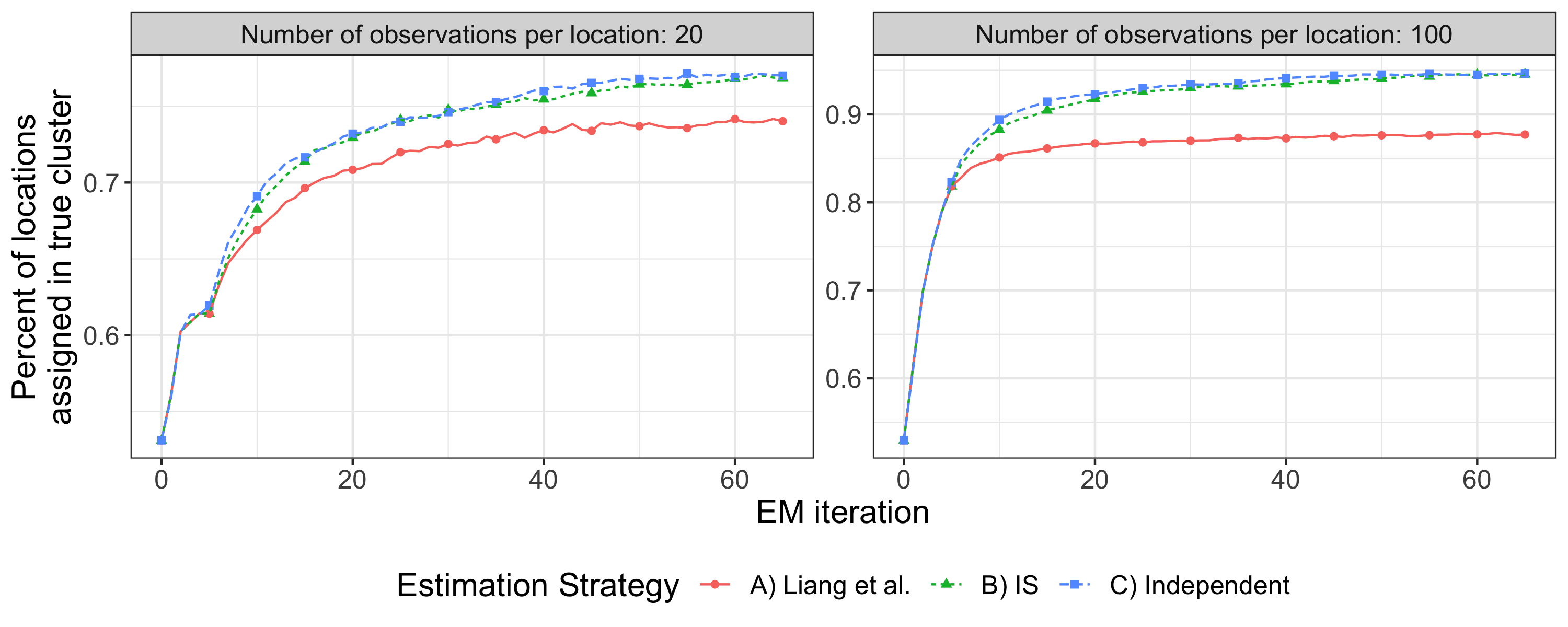
Figure 2: Percent of profiles correctly identified, averaged over simulations. The first 5 iterations are under the independent model for all models. IS refers to importance sampling.

4.2 Parameter Estimation

We consider $n=500$ locations and 200 observations per location. We create observations for two covariates with different mean functions. For the principal component functions, we create an orthogonal cubic spline basis $\{b_{1},\dots,b_{4}\}$ based on 2 equidistant knots on $[0,1]$, and use as multivariate principal component functions $\psi_{i}(\cdot)=2^{-1/2}(b_{i}(\cdot),b_{4-i+1}(\cdot))),~{}i=1,\dots,4$. For the means, we use $\mu_{\mathcal{Y}}(t)=\mu_{\mathcal{X}_{1}}(t)=e^{2-2t}\cos(5(t-0.1))$ and $\mu_{\mathcal{X}_{2}}(t)=5\cos(5t)$, and we use an orthogonal cubic spline basis $\{\phi_{1},\dots,\phi_{4}\}$ based on two equidistant knots on $[0,1]$ as principal component functions for the spatio-temporal random effect. Finally, we set $\mathscr{F}\psi_{1}(t)=1.5\sin(5(t+0.2))+t$, $\mathscr{F}\psi_{2}(t)=2\cos(7t)$, $\mathscr{F}\psi_{3}(t)=3\sin(-5.5(1-t))(1.1-t)^{2}$ and $\mathscr{F}\psi_{4}(t)=2e^{1-t}\log(1-t+0.1)+1$. The variances and spatial correlation parameters for the spatio-temporal random effect $\mathcal{E}$ are given in Table 1, along with their estimates. We select the penalty parameters and number of PCs based on (13), which chooses the correct number of response PCs 100% and predictor PCs 65% of the time. Figure 3 illustrates the resulting function estimates for $\mu_{\mathcal{Y}},\mathscr{F}\psi_{1},\mathscr{F}\psi_{4},\phi_{1},\phi_{2},\phi_{4}$. Overall, our MCEM algorithm appears to provide accurate estimates of the model parameters. Table 1 shows results for the variances and the spatial correlation scale parameters for the PCs of $\mathcal{E}$. Zhang, (2004) demonstrated that these parameters are not consistently estimable, however, consistent estimation of their ratio is possible and asymptotically, only the ratio matters for prediction. Our estimates of the ratio are reasonably unbiased. Plots of the remaining functions and the corresponding table for $\sigma_{\alpha,\ell}$ and $\kappa_{\alpha,\ell}$ are in the supplement Section S6.

$\ell$	$\sigma^{2}_{\eta,\ell}$	$\hat{\sigma}^{2}_{\eta,\ell}$	$\kappa_{\eta,\ell}$	$\hat{\kappa}_{\eta,\ell}$	$\sigma_{\eta,\ell}^{2}/\kappa_{\eta,\ell}$	$\hat{\sigma}^{2}_{\eta,\ell}/\hat{\kappa}_{\eta,\ell}$
1	$1.60$	1.46 (0.22)	$0.10$	0.09 (0.02)	$16$	15.92 (1.60)
2	$1.10$	1.05 (0.15)	$0.10$	0.09 (0.02)	$11$	11.85 (1.22)
3	$0.60$	0.57 (0.10)	$0.11$	0.10 (0.02)	$5.45$	5.94 (0.52)
4	$0.10$	0.10 (0.02)	$0.09$	0.08 (0.01)	$1.11$	1.29 (0.19)

Table 1: True and estimated parameters of the random fields of principal component scores for the spatio-temporal random effect $\mathcal{E}$. Numbers in brackets denote 1 empirical standard error based on 100 independent simulations.

Figure 3: Function approximation results from the simulation study of Section 4.2. Shaded region corresponds to 2 pointwise empirical standard deviations from the mean. (Top row, from left) The mean function $\mu_{\mathcal{Y}}$, then $\mathscr{F}\psi_{1},$ and $\mathscr{F}\psi_{4}$. (Bottom row) The principal component functions $\phi_{1},\phi_{2}$ and $\phi_{4}$ of the spatio-temporal random effect $\mathcal{E}$.

5 Data Analysis

In this section, we present the implementation and results on the Argo data in the Southern Ocean. We focus on this area since a large proportion of the biogeochemical (BGC) Argo data has been collected under the Southern Ocean Carbon and Climate Observations and Modeling (SOCCOM) project (Johnson et al.,, 2020, soccom.princeton.edu). For two overviews of the biogeochemical Argo program, see Bittig et al., (2019) and Claustre et al., (2020). We focus on oxygen data, though we also provide results for nitrate in Section S11. Argo data quality control for oxygen is described in Maurer et al., (2021), and comprehensive analyses of oceanic oxygen include Keeling et al., (2010) and Stramma and Schmidtko, (2021). For model training, we use about $13{,}000$ BGC profiles which yields $1.6\times 10^{6}$ oxygen measurements and $1.5\times 10^{7}$ temperature and salinity measurements, while also building an auxiliary dataset of more than $150{,}000$ Core profiles to be used for prediction in Section 5.3. In Section S7, we describe in detail how we created these datasets.

As discussed in the introduction, each Argo profile is a collection of measurements taken at different depths in the ocean. Thus, here the index $t_{ij}$ corresponds to pressure (depth) in the ocean, while $s_{i}$ represents the spatio-temporal index of a profile. The functional data perspective has some advantages in this context: integrals and derivatives of depth are immediately available, irregular sampling is handled by flexible B-spline bases, and dimension reduction in depth makes computation manageable. Viewing the Argo data as functional data has been considered in more detail in Yarger et al., (2022).

To provide background, we give a brief review of related oceanographic literature. First, interest in clustering applications in oceanography has risen quickly in recent years. Clustering has been used to characterize variability (Rosso et al.,, 2020), evaluate ocean heat content (Maze et al.,, 2017), examine El Niño events (Houghton and Wilson,, 2020), and identify oceanographic fronts (Jones et al.,, 2019; Thomas et al.,, 2021; Chapman et al.,, 2020). Thus far, clustering methodology in oceanography has primarily consisted of Gaussian Mixture Models (for example, Rosso et al.,, 2020; Thomas et al.,, 2021) and k-means (Houghton and Wilson,, 2020). These models have not taken advantage of spatial dependence of cluster memberships or observed data, which precludes spatial prediction.

As the BGC Argo program has developed, approaches for estimating and predicting its BGC variables has been an important area of research. Our aims closely match the spirit of Giglio et al., (2018), who use a random forest to predict oxygen from temperature, salinity, and spatio-temporal information. Expanding upon their work, we provide predictions at all pressure levels along with predicted uncertainties. In different settings, oceanographic approaches to predict BGC variables includes multivariate analysis (Liang et al.,, 2018), linear regression (Williams et al.,, 2016), and machine learning (Bittig et al.,, 2018).

5.1 Modeling and Implementation

Here, we specify our choice of spatial correlation function and other aspects of the application. For each principal component score, we use the anisotropic covariance function

$$\mathbb{C}\textrm{ov}(\alpha_{g,\ell}(s),\alpha_{g,\ell}(s^{\prime}))=\sigma^{2}_{g,\alpha,\ell}\textrm{exp}\left(-\sqrt{\sin(\gamma(s,s^{\prime})/2)^{2}\kappa_{g,\alpha,\ell,s}^{-2}+|u-u^{\prime}|^{2}\kappa_{g,\alpha,\ell,u}^{-2}}\right),$$

where $\gamma(s,s^{\prime})$ is the angle in radians between warped locations $\tilde{s}$ and $\tilde{s}^{\prime}$, and $u$ and $u^{\prime}$ are the respective times of the two samples. The warping is defined by gradients of spherical harmonic functions of degree 2 following Guinness, (2021) and implemented in the R package GpGp (Guinness et al.,, 2021). The parameters are the variance $\sigma^{2}_{g,\alpha,\ell}>0$, the scales $\kappa_{g,\alpha,\ell,s}$ and $\kappa_{g,\alpha,\ell,u}>0$, and the parameters for the warping transformation. This is similar in spirit to the choice of correlation function in Kuusela and Stein, (2018) and later in Yarger et al., (2022) because it allows the range of dependence to vary flexibly in space and time.

We chose 13 predictor and 11 response principal components using AIC. See results in Figure S6. We choose $5$ clusters based on oceanographic evidence (Orsi et al.,, 1995; Chapman et al.,, 2020). For the Markov random field, we consider the $15$ nearest neighbors based on the distance $\textrm{dist}_{\textrm{long}}+3\textrm{dist}_{\textrm{lat}}+12\textrm{dist}_{\textrm{day of year}}$ in kilometers and days, which takes into account seasonality and reflects scientific knowledge that scales in the longitude direction are often longer than latitude (for example, Roemmich and Gilson,, 2009).

5.2 Hold-out Experiments

We assess the prediction performance of our model in two separate scenarios: leave-profile-out and leave-float-out. For leave-profile-out, we hold out oxygen data from 1/5 of BGC profiles using a random partition, train the model on the remaining data, predict the left-out oxygen data, and repeat this process for of the five sets in the partition. For leave-float-out, we follow a similar process, but we instead partition floats into 10 sets, so that we hold out all oxygen data from selected floats at a time. In the leave-profile-out setting, nearby oxygen data from the same float is available; the leave-float-out setting is more challenging since one can only use oxygen data from other floats. Since Argo floats either have or do not have BGC sensors, leave-float-out is closer to the practical cokriging setting.

We found that for held-out locations with temperature and salinity data available, there is virtually no variation in cluster assignment across Monte Carlo samples used for prediction. Consequently, there are no mixture components, and it is straightforward to construct confidence intervals using the resulting Gaussian distribution. We take the measurement error into account when constructing these confidence intervals.

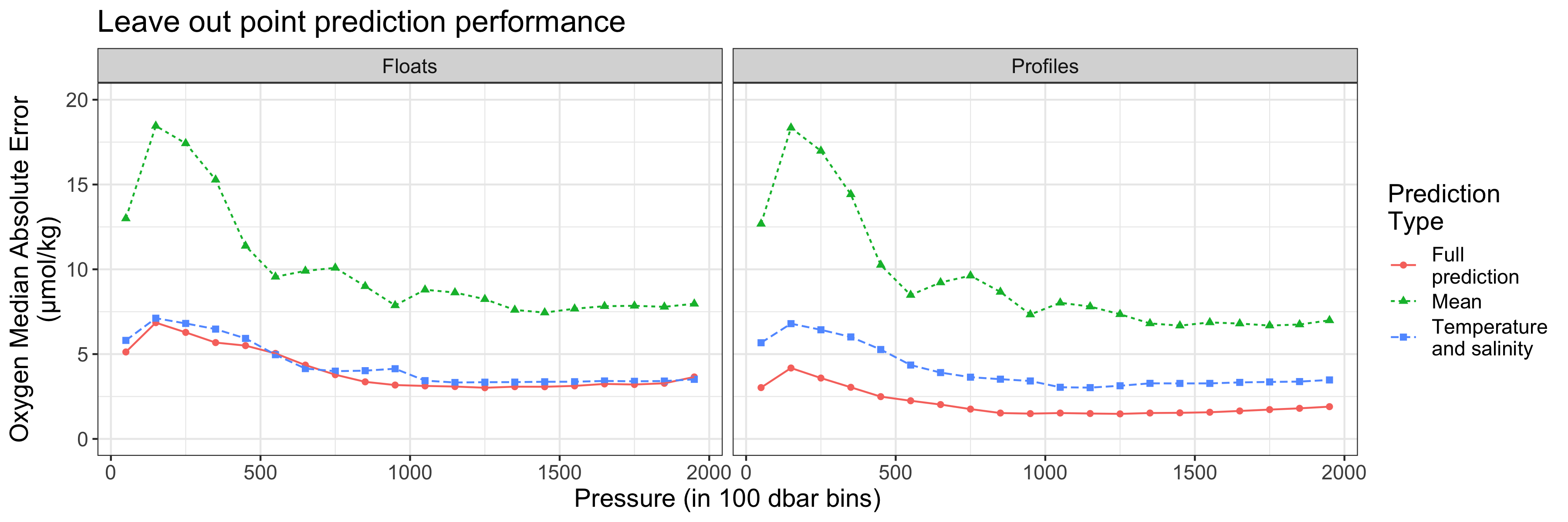
Figure 4: Median absolute error of oxygen (in $\mu$mol/kg) for leave-floats-out (Left) and leave-profiles-out (Right), summarized in 100 decibar bins. We compare predictions based on the cluster means only (“Mean”), the cluster means combined with temperature and salinity data (“Temperature and salinity”), and the full prediction (“Full prediction”).

In Figure 4, we plot the prediction error when using different components of the model. Temperature and salinity are present at each left-out profile, so the predictions based solely on covariates are comparable between cross validation settings. The abundance of nearby oxygen data can only be used by the full model in the leave-profile-out setting. The resulting prediction error is close to the instrument measurement error around 3 $\mu$mol/kg (Maurer et al.,, 2021; Mignot et al.,, 2019). Figure 5 describes the performance of our uncertainty estimates. In the leave-profile-out setting, the intervals are a bit conservative; in the leave-float-out setting, they are slightly too narrow. Generally, however, the uncertainty estimates appear to work well. Thus, our model can adapt its uncertainty estimates to varying sampling settings, which is especially promising as BGC float coverage increases.

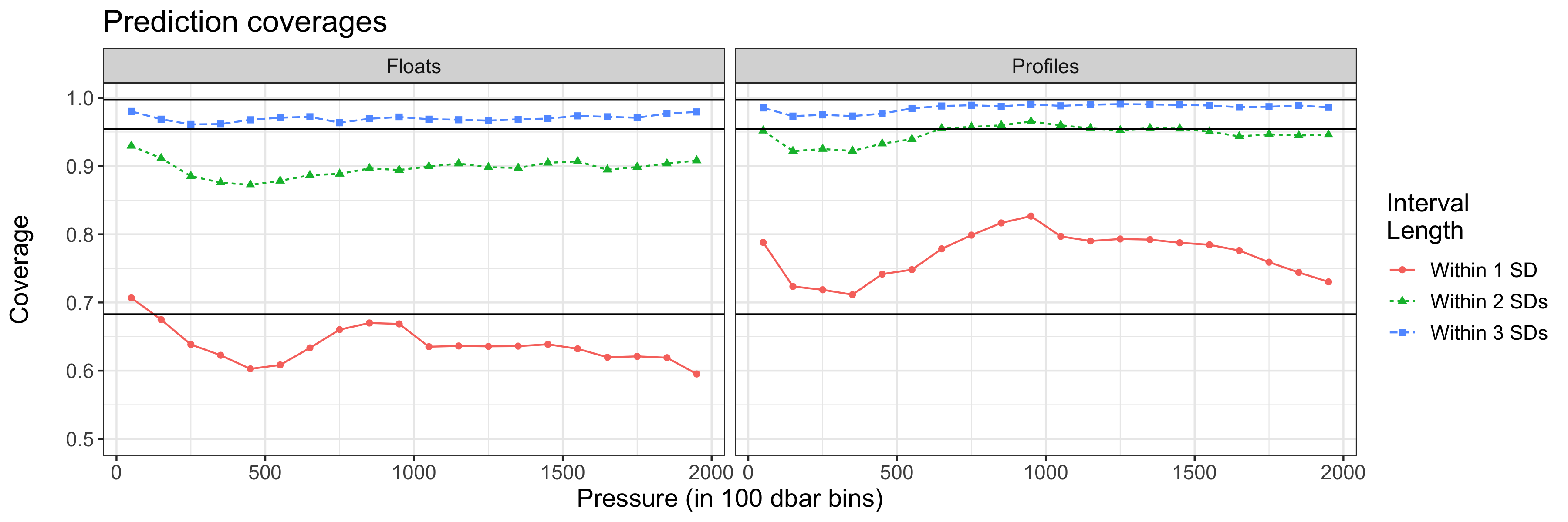
Figure 5: Interval coverages for intervals of 1, 2, and 3 standard deviations from the prediction, where the horizontal lines represent the nominal coverages.

We compare our approach with the random forest approach of Giglio et al., (2018). To assess prediction performance, we consider Argo measurements between 145 and 155 decibars and compare the point predictions for each held-out data experiment in Table 2. For the random forest, we use the parameters described in Giglio et al., (2018) on these measurements. In the leave-profile-out setting, the random forest easily modulates nearby profiles into the predictions well, and both approaches are comparable to the instrument measurement error. In the leave-float-out setting, the functional approach provides comparable predictions. In addition, we note that out-of-the-box implementation of the random forest as used in Giglio et al., (2018) does not supply uncertainty estimates, and computational issues arose when we applied it to data across all pressure levels. Finally, our model allows inference on its components including the clustering structure and the functional linear model as discussed next in Section 5.3.

Approach	Profile MAD ($\mu$mol/kg)	Profile RMSE ($\mu$mol/kg)	Float MAD ($\mu$mol/kg)	Float RMSE ($\mu$mol/kg)
RF	2.83	7.12	6.29	13.22
FC	4.32	10.49	7.14	14.85

Table 2: Comparison with random forest (RF) and functional cokriging (FC, our approach here) at 145-155 decibars. The median absolute deviation (MAD) and root-mean-squared-error (RMSE) are the metrics used for each of the methods and leave-out settings.

5.3 Recovery of Oceanographic Fronts and Prediction Product

We now present results from our extensive analysis of Biogeochemical and Core Argo data in the Southern Ocean, which is based on interpolation of cluster memberships and oxygen on a grid using the methodology developed in Section 3.3. This allows us to provide interpretable maps of oceanographic fronts and oxygen concentration. First, we provide a thorough analysis of heterogeneity in ocean properties based on oxygen, temperature, and salinity data. In Figure 6, we plot predictions of cluster memberships and their uncertainty. In addition, traditional estimates of fronts are plotted using the same criteria for fronts as Bushinsky et al., (2017) based on the 2004-2018 Roemmich and Gilson, (2009) estimate. Finally, we include the oxygen mean functions for each cluster.

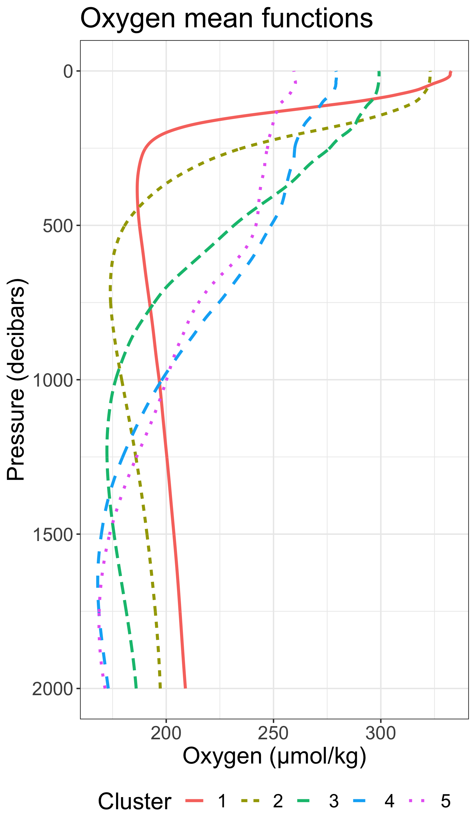
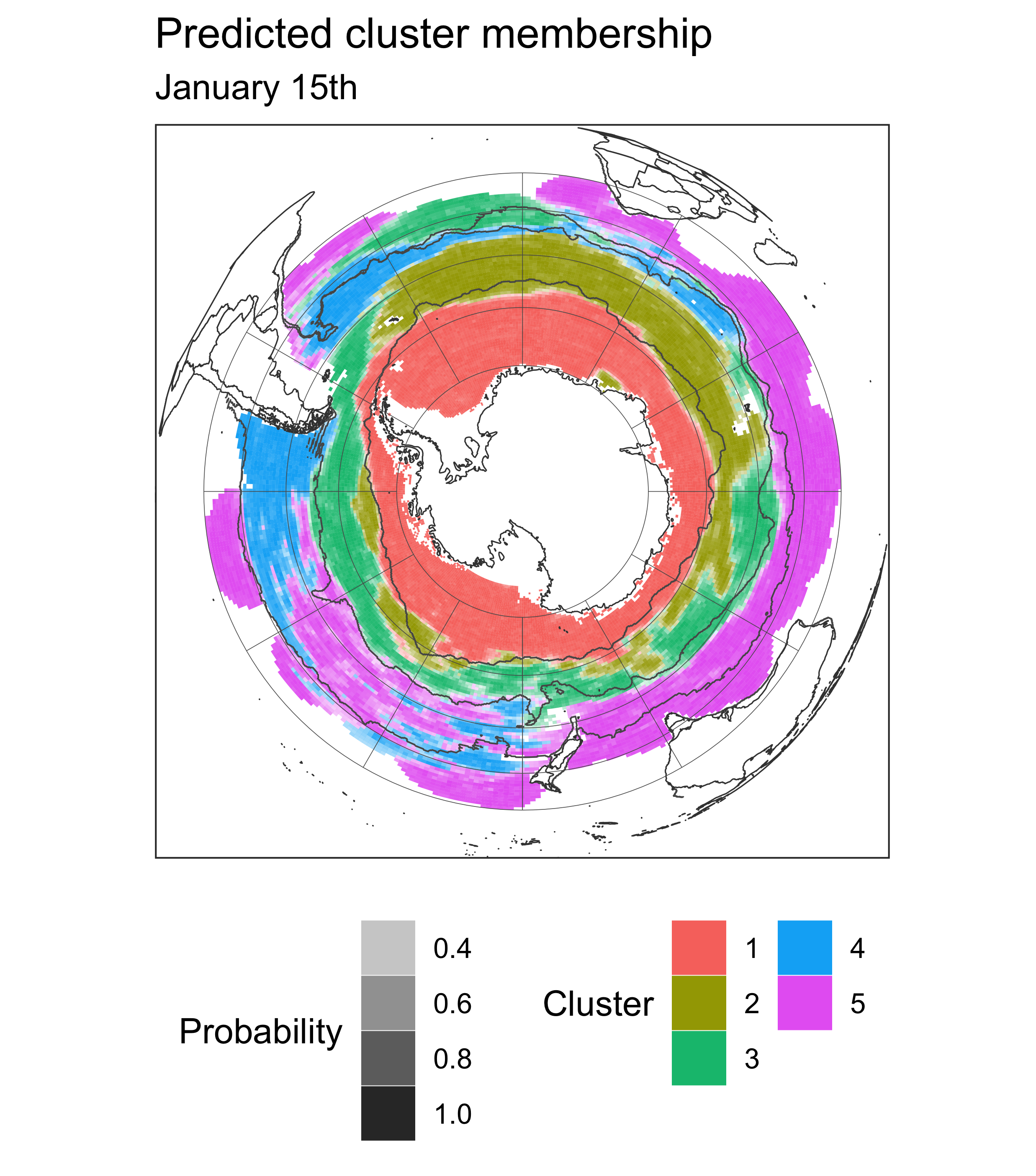
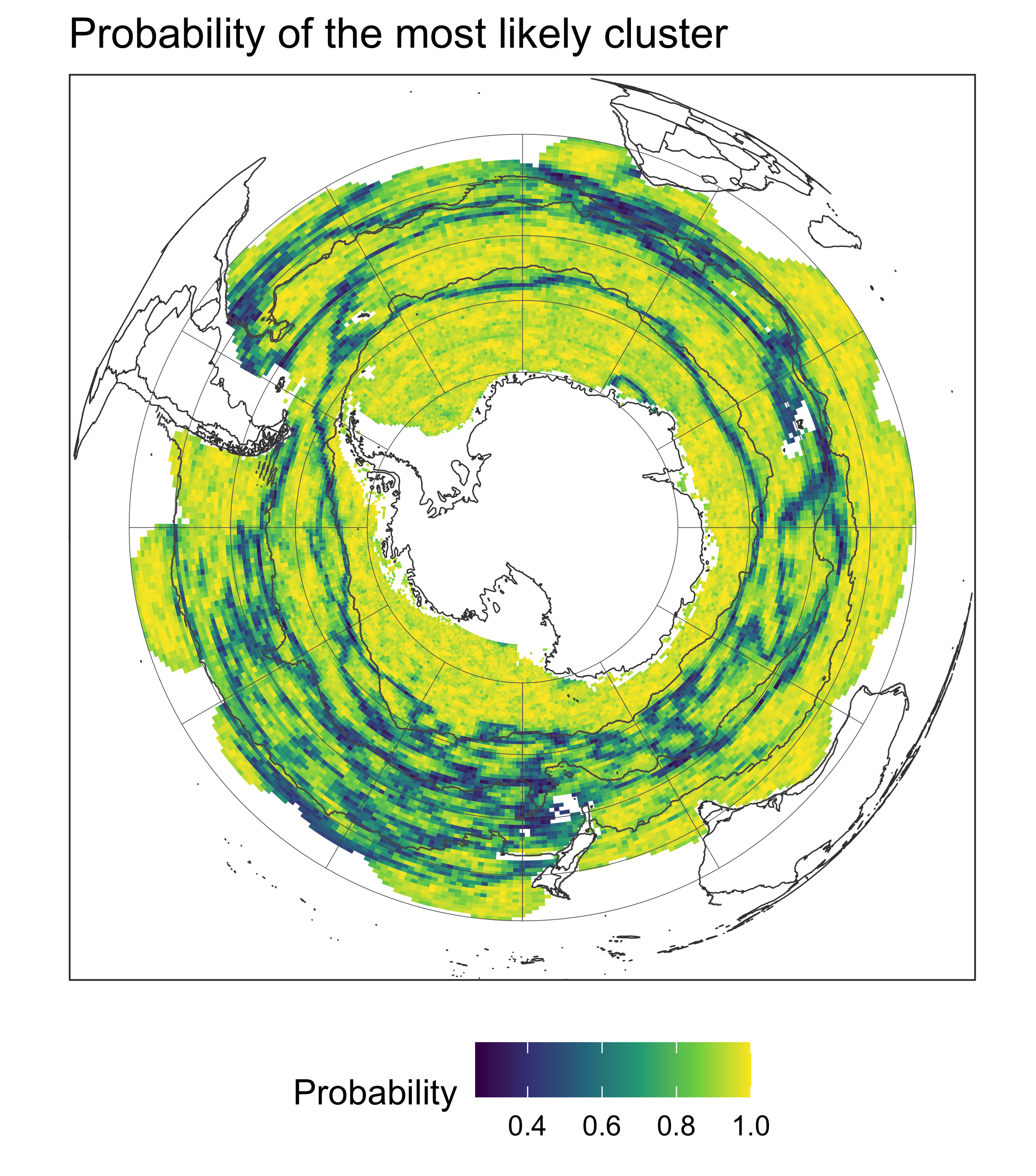
Figure 6: (Left) Oxygen mean functions of pressure for each cluster. (Middle) Marginal membership using the Markov random field for January 15th; grid opacity is determined by the probability of the most likely cluster, with the same colors as the mean functions. (Right) Probability of the most likely cluster for January 15th.

We focus on cluster predictions for the austral summer (e.g. January) because historically, more measurements are available during this season, making the comparison between our results and existing literature more relevant. The boundary of our first cluster defines the Southern Antarctic Circumpolar front, which closely matches that found in Orsi et al., (1995). Clusters 2 and 3 make up the main component of the Antarctic Circumpolar Current, with their northern boundary aligning with the subantarctic front. Clusters 4 and 5 define waters above the subantarctic front, with cluster 4 more concentrated in the Pacific. Our approach also allows us to model behavior of fronts in other seasons (see Figure S5). Interestingly, for other seasons there is less agreement, indicating dynamic behavior of fronts. Similar to the “I-metric” of Thomas et al., (2021), we provide uncertainty estimates of the clusters as shown in Figure 6, while also characterizing using Equation (11) how this uncertainty contributes to that of the oxygen predictions, plotted in Figure S16.

To provide a set of oxygen predictions that can be used by scientists, we predict for each month of the year from July 2014 to June 2020. As an example in Figure 7, we plot oxygen predictions and their standard deviations at 150 decibars for January 15th, 2020, taking advantage of our functional approach that provides predictions at arbitrary pressure levels. We then provide the predictions, their variances, and the averaged fields in a product in netcdf form, given in Section S10. We provide more prediction plots in Section S11.

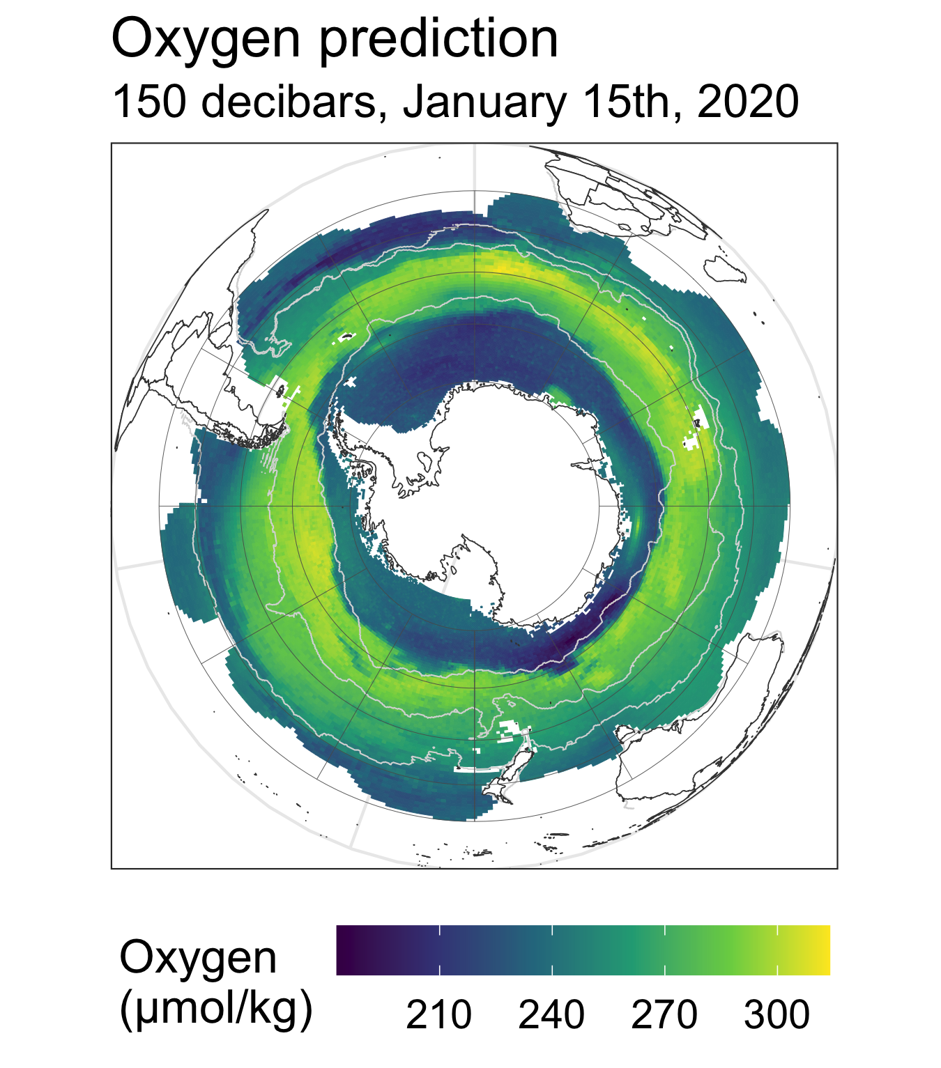
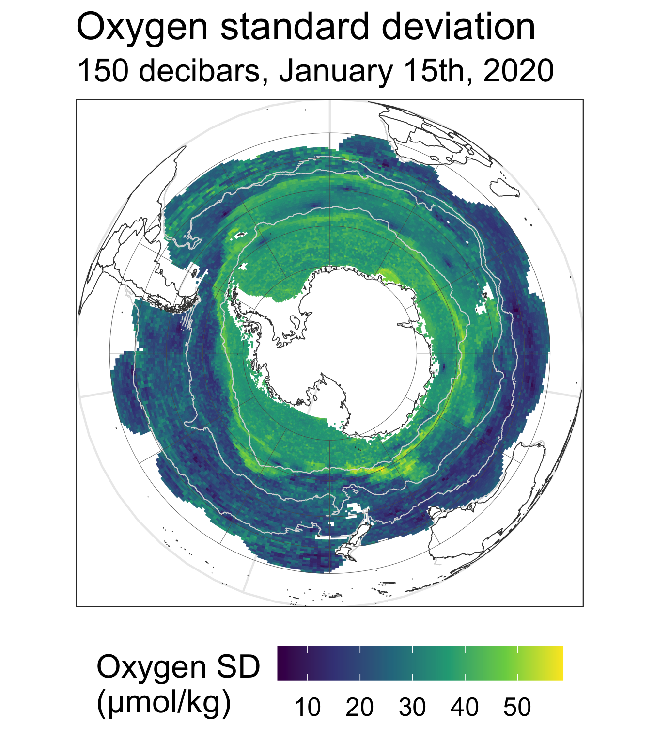
Figure 7: (Left) Prediction $\widehat{\mathcal{Y}(\check{\boldsymbol{s}},t)}$ on a grid for January 15th, 2020 and $t=150$ decibars. (Right) Prediction standard deviations for the same quantities.

6 Discussion

In this work, we introduce a model for multivariate and spatio-temporal functional data that enables large-scale cokriging (spatio-temporal prediction). The model simultaneously handles multivariate functional data, spatio-temporal dependence, and heterogeneous spatial features through a latent clustering structure. We introduce an importance-sampling-based Monte Carlo EM algorithm for model estimation that overcomes computational and inferential challenges faced by existing methodologies, as demonstrated in a simulation study. We contribute methodology for spatio-temporal prediction that takes into account uncertainty in cluster memberships. Among other methodological advances that make adaptation to large amounts of data possible, we avoid use of orthogonal B-splines, providing a framework that is more efficient in computation and memory. Our code and approach for estimation can be adapted for data in neuroscience or elsewhere in environmental sciences.

A number of extensions and applications of our methodology remain. For example, functional canonical correlation analysis may better represent the relationship between the covariates and the response. The current model is also developed with independence assumed between different clusters; incorporating dependence between clusters may better represent available data. Including scalar covariates like satellite data in the model is straightforward and may be of practical interest. Finally, using more sophisticated model selection for the Markov random field might improve the cluster predictions.

We use our framework for a large-scale data analysis on the biogeochemical Argo data in the Southern Ocean. Via hold-out experiments and a comparison with existing approaches, we demonstrate that our model provides accurate predictions of oxygen data as well as reliable estimates of variability. Our clustering results independently recover established oceanographic fronts and provide insights into the spatio-temporal dynamics of these fronts. Statistical approaches like the one developed here will play an important role for the analysis of data from the planned global deployment of BGC Argo floats (see NSF Award 1946578).

SUPPLEMENTARY MATERIAL

S1 Conditional Distributions

Here, we provide the conditional distributions required for our MCEM algorithm. The first proposition gives the conditional distribution of the observed data given the latent field $\{Z(s_{i})\}_{i=1}^{n}$ in various scenarios. In the following, for arbitrary matrices $A_{1},\dots,A_{M}$, let bdiag($A_{1},\dots,A_{M}$) denote the block diagonal matrix with the matrices $A_{1},\dots,A_{M}$ on the diagonal.

Proposition 1.

Let $\alpha$ be a normally distributed random vector of size $m_{1}$ with mean 0 and covariance $\Sigma_{\alpha}$. Let $\eta$ be another normally distributed random vector of size $m_{2}$ with mean 0 and covariance $\Sigma_{\eta}$. Furthermore, let $\epsilon_{X}$ and $\epsilon_{Y}$ by two random vectors with

$$\epsilon_{Y}\sim\mathcal{N}(0,\sigma_{Y}^{2}I_{N_{2}})~{}~{}\text{ and }~{}~{}\epsilon_{X}\sim\mathcal{N}\left(0,\mathrm{bdiag}(\sigma_{X_{1}}^{2}I_{n^{1}},\dots,\sigma_{X_{K}}^{2}I_{n^{K}})\right)=:\mathcal{N}\left(0,D_{X}\right),$$

where the parameters $\sigma_{Y}^{2}>0$ and $\sigma_{X_{k}}^{2}>0$ for $k=1,\dots,K$ are measurement error variances. Assume that $\alpha,\eta,\epsilon_{X}$ and $\epsilon_{Y}$ are mutually independent of each other. Let $N_{1}=\sum_{k=1}^{K}n^{k}$ and assume $\min(N_{1},N_{2})>\max(m_{1},m_{2})$. Furthermore, let $A_{1},A_{2},A_{3}$ be three matrices of dimensions $N_{1}\times m_{1}$, $N_{2}\times m_{1}$ and $N_{2}\times m_{2}$ respectively. Define

$$X =A_{1}\alpha+\epsilon_{X}, Y =A_{2}\alpha+A_{3}\eta+\epsilon_{Y}.$$

Then

$$\begin{pmatrix}X\\ Y\end{pmatrix}\sim\mathcal{N}\left(0,\begin{pmatrix}D_{X}+A_{1}\Sigma_{\alpha}A_{1}^{\top}&A_{1}\Sigma_{\alpha}A_{2}^{\top}\\ A_{2}\Sigma_{\alpha}A_{1}^{\top}&\sigma_{Y}^{2}I_{n_{2}}+A_{2}\Sigma_{\alpha}A_{2}^{\top}+A_{3}\Sigma_{\eta}A_{3}^{\top}\end{pmatrix}\right).$$

Proof.

The proof follows directly from standard properties of the normal distribution. ∎

Next, we derive the conditional density $f(\boldsymbol{\alpha},\boldsymbol{\eta}|\boldsymbol{X},\boldsymbol{Y},\boldsymbol{Z})$. As observations from different clusters are assumed to be independent, it suffices to derive the distribution for specific cluster. Thus to ease notation, we drop cluster dependence.

Proposition 2.

Let $B_{i}$ be the $n_{i}\times P$ matrix of basis evaluations for profile $i$ for the response. Similarly, let $\boldsymbol{B}_{i}$ be the respective $Kn_{i}\times KP$ be the respective matrix for the covariates, which is the block-diagonal matrix of evaluations for each predictor. Write $\tilde{\boldsymbol{B}}=\mathrm{bdiag}(B_{1},\dots,B_{n})$ and $\boldsymbol{B}=\mathrm{bdiag}(\boldsymbol{B}_{1},\dots,\boldsymbol{B}_{n})$. For any matrix or vector $\Theta$ with appropriate dimension, write

$$\boldsymbol{B}\Theta=\mathrm{bdiag}(\boldsymbol{B}_{1}\Theta,\dots\boldsymbol{B}_{n}\Theta)~{}~{}~{}\text{ and }\tilde{\boldsymbol{B}}\Theta=\mathrm{bdiag}(B_{1}\Theta,\dots B_{n}\Theta)$$

as well as $D_{X}=\mathrm{bdiag}\left(D_{X^{1}},\dots,D_{X^{n}}\right)$ where $D_{X^{i}}=\mathbb{V}\textrm{ar}\left[\left(\epsilon_{i1}^{1},\dots,\epsilon_{in_{i}}^{1},\dots,\epsilon_{i1}^{K},\dots,\epsilon_{in_{i}}^{K}\right)\right]$. For the response, let $\sigma^{2}_{Y}=\mathbb{V}\textrm{ar}(\epsilon_{11}^{Y})$. In addition, let $\Sigma_{\alpha}=\mathbb{V}\textrm{ar}(\boldsymbol{\alpha})$ and $\Sigma_{\eta}=\mathbb{V}\textrm{ar}(\boldsymbol{\eta})$ be defined by the spatial covariance.

Within the same cluster, we have

$$\boldsymbol{\alpha},\boldsymbol{\eta}|\boldsymbol{X},\boldsymbol{Y}\sim\mathcal{N}\left(\begin{pmatrix}\mu_{\alpha}\\ \mu_{\eta}\end{pmatrix},\begin{pmatrix}\Sigma_{\alpha,\alpha}&\Sigma_{\alpha,\eta}\\ \Sigma_{\eta,\alpha}&\Sigma_{\eta,\eta}\end{pmatrix}\right)=\mathcal{N}\left(\begin{pmatrix}\mu_{\alpha}\\ \mu_{\eta}\end{pmatrix},\Sigma\right)$$

with

$$\Sigma^{-1}=\begin{pmatrix}\Sigma_{\alpha}^{-1}+(\boldsymbol{B}\Theta_{\mathcal{X}})^{\top}D_{X}^{-1}\boldsymbol{B}\Theta_{\mathcal{X}}+\sigma_{Y}^{-2}(\tilde{\boldsymbol{B}}\Lambda)^{\top}\tilde{\boldsymbol{B}}\Lambda&\sigma_{Y}^{-2}(\tilde{\boldsymbol{B}}\Lambda)^{\top}\tilde{\boldsymbol{B}}\Theta_{\mathcal{E}}\\ (\sigma_{Y}^{-2}(\tilde{\boldsymbol{B}}\Lambda)^{\top}\tilde{\boldsymbol{B}}\Theta_{\mathcal{E}})^{\top}&\Sigma_{\eta}^{-1}+\sigma_{Y}^{-2}(\tilde{\boldsymbol{B}}\Theta_{\mathcal{E}})^{\top}\tilde{\boldsymbol{B}}\Theta_{\mathcal{E}}\end{pmatrix}$$

and

$$\mu_{\alpha} =\Sigma_{\alpha,\alpha}\left[(\boldsymbol{B}\Theta_{\mathcal{X}})^{\top}D_{X}^{-1}(\boldsymbol{X}-\boldsymbol{B}\theta_{\mathcal{X}})+\sigma_{Y}^{-2}(\tilde{\boldsymbol{B}}\Lambda)^{\top}(\boldsymbol{Y}-\tilde{\boldsymbol{B}}\theta_{\mathcal{Y}})\right]$$

$$~{}~{}~{}+\Sigma_{\alpha,\eta}\sigma_{Y}^{-2}(\tilde{\boldsymbol{B}}\Theta_{\mathcal{E}})^{\top}(\boldsymbol{Y}-\tilde{\boldsymbol{B}}\theta_{\mathcal{Y}})$$

$$\mu_{\eta} =\Sigma_{\eta,\eta}\left[\sigma_{Y}^{-2}(\tilde{\boldsymbol{B}}\Theta_{\mathcal{E}})^{\top}(\boldsymbol{Y}-\tilde{\boldsymbol{B}}\theta_{\mathcal{Y}})\right]$$

$$~{}~{}~{}+\Sigma_{\eta,\alpha}\left[(\boldsymbol{B}\Theta_{\mathcal{X}})^{\top}D_{X}^{-1}(\boldsymbol{X}-\boldsymbol{B}\theta_{\mathcal{X}})+\sigma_{Y}^{-2}(\tilde{\boldsymbol{B}}\Lambda)^{\top}(\boldsymbol{Y}-\tilde{\boldsymbol{B}}\theta_{\mathcal{Y}})\right].$$

Here, $\Theta_{\mathcal{E}}$, $\Lambda$, and $\Theta_{\mathcal{X}}$ are the respective matrices for the principal component/random effect function coefficients and $\theta_{\mathcal{X}}$ and $\theta_{\mathcal{Y}}$ are the respective vectors for the mean coefficients, ignoring notation on the cluster.

Proof of Proposition 2.

We have

$$f {}_{\boldsymbol{\alpha},\boldsymbol{\eta}|\boldsymbol{X},\boldsymbol{Y}}(\boldsymbol{\alpha},\boldsymbol{\eta})\propto f_{\boldsymbol{X}|\boldsymbol{\alpha}}(\boldsymbol{X})f_{\boldsymbol{Y}|\boldsymbol{\alpha},\boldsymbol{\eta}}(\boldsymbol{Y})f_{\boldsymbol{\alpha}}(\boldsymbol{\alpha})f_{\boldsymbol{\eta}}(\boldsymbol{\eta})$$

$$\propto\exp\left(-\frac{1}{2}\sum_{i=1}^{n}(\boldsymbol{X}_{i}-\boldsymbol{B}_{i}(\theta_{\mathcal{X}}+\Theta_{\mathcal{X}}\boldsymbol{\alpha}_{i}))^{\top}D_{X^{i}}^{-1}(\boldsymbol{X}_{i}-\boldsymbol{B}_{i}(\theta_{\mathcal{X}}+\Theta_{\mathcal{X}}\boldsymbol{\alpha}_{i}))\right)$$

$$~{}~{}~{}~{}\times\exp\left(-\frac{1}{2\sigma_{Y}^{2}}\sum_{i=1}^{n}\left\lVert\boldsymbol{Y}_{i}-B_{i}(\theta_{\mathcal{Y}}+\Lambda\boldsymbol{\alpha}_{i}+\Theta_{\mathcal{E}}\boldsymbol{\eta}_{i})\right\rVert^{2}\right)\exp\left(-\frac{1}{2}\boldsymbol{\eta}^{\top}\Sigma_{\eta}^{-1}\boldsymbol{\eta}\right)$$

$$~{}~{}~{}~{}\times\exp\left(-\frac{1}{2}\boldsymbol{\alpha}^{\top}\Sigma_{\alpha}^{-1}\boldsymbol{\alpha}\right)$$

$$\propto\exp\left(-\frac{1}{2}\begin{pmatrix}\boldsymbol{\alpha}\\ \boldsymbol{\eta}\end{pmatrix}^{\top}\begin{pmatrix}\Sigma_{\alpha}^{-1}+(\boldsymbol{B}\Theta_{\mathcal{X}})^{\top}D_{X}^{-1}\boldsymbol{B}\Theta_{\mathcal{X}}+\sigma_{Y}^{-2}(\tilde{\boldsymbol{B}}\Lambda)^{\top}\tilde{\boldsymbol{B}}\Lambda&\sigma_{Y}^{-2}(\tilde{\boldsymbol{B}}\Lambda)^{\top}\tilde{\boldsymbol{B}}\Theta_{\mathcal{E}}\\ (\sigma_{Y}^{-2}(\tilde{\boldsymbol{B}}\Lambda)^{\top}\tilde{\boldsymbol{B}}\Theta_{\mathcal{E}})^{\top}&\Sigma_{\eta}^{-1}+\sigma_{Y}^{-2}(\tilde{\boldsymbol{B}}\Theta_{\mathcal{E}})^{\top}\tilde{\boldsymbol{B}}\Theta_{\mathcal{E}}\end{pmatrix}\begin{pmatrix}\boldsymbol{\alpha}\\ \boldsymbol{\eta}\end{pmatrix}\right)$$

$$~{}~{}~{}~{}\times\exp\left(\boldsymbol{\alpha}^{\top}\left[D_{X}^{-1}(\boldsymbol{B}\Theta_{\mathcal{X}})^{\top}(\boldsymbol{B}\theta_{\mathcal{X}}-\boldsymbol{X})+\sigma_{Y}^{-2}(\tilde{\boldsymbol{B}}\Lambda)^{\top}(\tilde{\boldsymbol{B}}\theta_{\mathcal{Y}}-\boldsymbol{Y})\right]\right)$$

$$~{}~{}~{}~{}\times\exp\left(\boldsymbol{\eta}^{\top}\left[\sigma_{Y}^{-2}(\tilde{\boldsymbol{B}}\Theta_{\mathcal{E}})^{\top}(\tilde{\boldsymbol{B}}\theta_{\mathcal{Y}}-\boldsymbol{Y})\right]\right)$$

$$=\exp\left(-\frac{1}{2}(\boldsymbol{\alpha}^{\top},\boldsymbol{\eta}^{\top})\Sigma^{-1}\begin{pmatrix}\boldsymbol{\alpha}\\ \boldsymbol{\eta}\end{pmatrix}\right)\exp\left((\boldsymbol{\alpha}^{\top},\boldsymbol{\eta}^{\top})\Sigma^{-1}\begin{pmatrix}\mu_{\alpha}\\ \mu_{\eta}\end{pmatrix}\right)$$

from which we obtain the inverse covariance matrix immediately. Let $\Sigma_{\alpha,\alpha}^{\mathrm{inv}},\Sigma_{\alpha,\alpha}^{\mathrm{inv}}$ and $\Sigma_{\eta,\eta}^{\mathrm{inv}}$ denote the blocks of $\Sigma^{-1}$. Then comparing the expression involving the means, we obtain

$$\Sigma^{-1}\begin{pmatrix}\mu_{\alpha}\\ \mu_{\eta}\end{pmatrix} =\begin{pmatrix}\Sigma_{\alpha,\alpha}^{\mathrm{inv}}\mu_{\alpha}+\Sigma^{\mathrm{inv}}_{\alpha,\eta}\mu_{\eta}\\ \Sigma_{\eta,\alpha}^{\mathrm{inv}}\mu_{\alpha}+\Sigma^{\mathrm{inv}}_{\eta,\eta}\mu_{\eta}\end{pmatrix}$$

$$=\begin{pmatrix}(\boldsymbol{B}\Theta_{\mathcal{X}})^{\top}D_{X}^{-1}(\boldsymbol{X}-\boldsymbol{B}\theta_{\mathcal{X}})+\sigma_{Y}^{-2}(\tilde{\boldsymbol{B}}\Lambda)^{\top}(\boldsymbol{Y}-\tilde{\boldsymbol{B}}\theta_{\mathcal{Y}})\\ \sigma_{Y}^{-2}(\tilde{\boldsymbol{B}}\Theta_{\mathcal{E}})^{\top}(\boldsymbol{Y}-\tilde{\boldsymbol{B}}\theta_{\mathcal{Y}}),\end{pmatrix}$$

and solving for $\mu_{\alpha},\mu_{\eta}$ yields

$$\mu_{\alpha} =\Sigma_{\alpha,\alpha}\left[(\boldsymbol{B}\Theta_{\mathcal{X}})^{\top}D_{X}^{-1}(\boldsymbol{X}-\boldsymbol{B}\theta_{\mathcal{X}})+\sigma_{Y}^{-2}(\tilde{\boldsymbol{B}}\Lambda)^{\top}(\boldsymbol{Y}-\tilde{\boldsymbol{B}}\theta_{\mathcal{Y}})\right]$$

$$~{}~{}~{}~{}~{}+\Sigma_{\alpha,\eta}\left[\sigma_{Y}^{-2}(\tilde{\boldsymbol{B}}\Theta_{\mathcal{E}})^{\top}(\boldsymbol{Y}-\tilde{\boldsymbol{B}}\theta_{\mathcal{Y}})\right],$$

$$\mu_{\eta} =\Sigma_{\eta,\eta}\left[\sigma_{Y}^{-2}(\tilde{\boldsymbol{B}}\Theta_{\mathcal{E}})^{\top}(\boldsymbol{Y}-\tilde{\boldsymbol{B}}\theta_{\mathcal{Y}})\right]$$

$$~{}~{}~{}~{}~{}+\Sigma_{\eta,\alpha}\left[(\boldsymbol{B}\Theta_{\mathcal{X}})^{\top}D_{X}^{-1}(\boldsymbol{X}-\boldsymbol{B}\theta_{\mathcal{X}})+\sigma_{Y}^{-2}(\tilde{\boldsymbol{B}}\Lambda)^{\top}(\boldsymbol{Y}-\tilde{\boldsymbol{B}}\theta_{\mathcal{Y}})\right].$$

∎

S2 Computation of Conditional Distributions

Consider the notation in Section S1, and note that our goal is to sample from $f(\boldsymbol{\alpha},\boldsymbol{\eta}|\boldsymbol{X},\boldsymbol{Y})$ efficiently. All distributions should be considered conditional on $\boldsymbol{Z}$, but this notation is omitted as in Section S1. Defining

$$U:=\begin{pmatrix}D_{X}^{-1/2}\boldsymbol{B}\Theta_{\mathcal{X}}&0\\ \sigma_{Y}^{-1}\tilde{\boldsymbol{B}}\Lambda&\sigma_{Y}^{-1}\tilde{\boldsymbol{B}}\Theta_{\mathcal{E}}\end{pmatrix}~{}\text{ and }~{}A:=\begin{pmatrix}\Sigma_{\alpha}&0\\ 0&\Sigma_{\eta}\end{pmatrix},$$ (14)

we may write

$$\Sigma^{-1}=A^{-1}+U^{\top}U.$$

In practice, $\Sigma^{-1}$ will be considerably sparse due to the independence assumption on the scores; furthermore, one can apply popular sparse matrix spatial statistics approximations to $A^{-1}$, like Vecchia’s approximation (Guinness,, 2021). We next form the Cholesky matrix of $\Sigma^{-1}=LL^{\top}$, which is the largest computation in the E-step. Then:

1. The conditional mean of $\boldsymbol{\alpha},\boldsymbol{\eta}|\boldsymbol{X},\boldsymbol{Y}$ can be found by backsolving and forwardsolving using $L$.

2. A mean-zero random normal vector with covariance $\Sigma$ can be generated by backsolving against a vector with independent standard normal entries using $L$.

3. The marginal likelihood of $\boldsymbol{X}$ and $\boldsymbol{Y}$ (once again conditional on cluster memberships) can be computed, which factor into the importance sample weights. That is, write

   $$\boldsymbol{X}_{0} =\boldsymbol{X}-\boldsymbol{B}\theta_{\mathcal{X}},$$

   $$\boldsymbol{Y}_{0} =\boldsymbol{Y}-\tilde{\boldsymbol{B}}\theta_{\mathcal{Y}},$$

   $$D_{X,Y} =\textrm{diag}\left(D_{X}^{1/2},\sigma_{Y}I_{\sum_{i=1}^{n}n_{i}}\right),$$

   $$\Sigma_{\textrm{data}}=\mathbb{V}\textrm{ar}\left(\begin{matrix}\boldsymbol{X}\\ \boldsymbol{Y}\end{matrix}\middle|\Omega\right) =D_{X,Y}UAU^{\top}D_{X,Y}+D_{X,Y}^{2}.$$

   Finally, write $n_{\textrm{data}}=(K+1)\sum_{i=1}^{n}n_{i}$ as the number of total observed measurements, so that

   $$\ell(\Omega,\boldsymbol{X},\boldsymbol{Y})=-\frac{1}{2}\left(\log(2\pi)n_{\textrm{data}}+\log(|\Sigma_{\textrm{data}}|)+\left(\boldsymbol{X}_{0}^{\top},\boldsymbol{Y}_{0}^{\top}\right)\Sigma_{\textrm{data}}^{-1}\begin{pmatrix}\boldsymbol{X}_{0}\\ \boldsymbol{Y}_{0}\end{pmatrix}\right)$$

   where $|\Sigma_{\textrm{data}}|$ denotes the determinant of $\Sigma_{\textrm{data}}$. Using the matrix determinant lemma,

   $$|\Sigma_{\textrm{data}}| =\left|A^{-1}+U^{\top}U\right|\left|A^{-1}\right|^{-1}\left|D_{X,Y}^{2}\right|.$$

   The first determinant can be computed quickly from $L$, the second is quickly available when using a Vecchia approximation, and the final determinant (of a diagonal matrix) can also be computed quickly. Using the Woodbury matrix identity,

   $$\begin{pmatrix}\boldsymbol{X}_{0}\\ \boldsymbol{Y}_{0}\end{pmatrix}^{\top}\Sigma_{\textrm{data}}^{-1}\begin{pmatrix}\boldsymbol{X}_{0}\\ \boldsymbol{Y}_{0}\end{pmatrix} =\begin{pmatrix}\boldsymbol{X}_{0}\\ \boldsymbol{Y}_{0}\end{pmatrix}^{\top}\left(D_{X,Y}^{-2}-D_{X,Y}^{-1}U\left(A^{-1}+U^{\top}U\right)^{-1}U^{\top}D_{X,Y}^{-1}\right)\begin{pmatrix}\boldsymbol{X}_{0}\\ \boldsymbol{Y}_{0}\end{pmatrix}$$

   $$=\left\lVert D_{X,Y}^{-1}\begin{pmatrix}\boldsymbol{X}_{0}\\ \boldsymbol{Y}_{0}\end{pmatrix}\right\rVert^{2}-\boldsymbol{V}^{\top}\left(A^{-1}+U^{\top}U\right)^{-1}\boldsymbol{V},$$

   where $\boldsymbol{V}=U^{\top}D_{X,Y}^{-1}\begin{pmatrix}\boldsymbol{X}_{0}\\ \boldsymbol{Y}_{0}\end{pmatrix}$. The first term can be quickly computed, and the second term’s only computational challenge is back/forward solving against $L$.

   After tailoring this likelihood computation to a particular clustering $\boldsymbol{Z}$, this solves the evaluation of $f(\boldsymbol{X},\boldsymbol{Y}|\boldsymbol{Z})$ in the importance sampling weights. Also, evaluation of $f(\boldsymbol{X}_{i},\boldsymbol{Y}_{i}|Z_{i})$ can be done similarly.

These three computational derivations allow working with matrices the size of the total number of principal component scores, rather than the total number of data points. In practice, creating a permuted Cholesky matrix also improves sparsity and computation speed.

S3 Illustration with Gibbs Sampling

Here, we discuss the Gibbs sampling approach proposed by Liang et al., (2020) and reviewed in Section 3.2. While the Gibbs sampling approach works suitably when there are only a few measurements per location, when there are many measurements per location, the Gibbs approach does not mix well since $\boldsymbol{Z}^{(\tau-1)}$ and $\boldsymbol{Z}^{(\tau)}$ are strongly correlated for $\tau=2,\dots,T$. To illustrate, assume $\boldsymbol{\alpha}_{i}^{(\tau)}$ and $\boldsymbol{\eta}_{i}^{(\tau)}$ were drawn based on $Z_{i}^{(\tau-1)}=g$. Then for any $g^{\prime}\neq g$, the approximation $\boldsymbol{Y}_{i}-B_{i}\theta_{g^{\prime},\mathcal{Y}}\approx B_{i}\Lambda_{g^{\prime}}\boldsymbol{\alpha}_{i}^{(\tau)}+B_{i}\Theta_{g^{\prime}}\boldsymbol{\eta}_{i}^{(\tau)}$ is poor if $\theta_{g}$ and $\theta_{g^{\prime}}$, $\Lambda_{g}$ and $\Lambda_{g^{\prime}}$, or $\Theta_{g}$ and $\Theta_{g^{\prime}}$ are substantially different. This is the case even if the covariance structures are the same in every cluster but the means are different. Consequently, $\mathbb{P}\left(Z_{i}\neq g\middle|\boldsymbol{\alpha}_{i}^{(\tau)},\boldsymbol{\eta}_{i}^{(\tau)},\boldsymbol{X}_{i},\boldsymbol{Y}_{i}\right)$, which depends heavily on

$$\left\lVert\boldsymbol{Y}_{i}-B_{i}\theta_{g,\mathcal{Y}}-B_{i}\Lambda_{g}\boldsymbol{\alpha}_{i}^{(\tau)}-B_{i}\Theta_{g}\boldsymbol{\eta}_{i}^{(\tau)}\right\rVert$$

and the respective quantities for the covariates, will be vanishingly small. This in turn will lead to high correlation of the samples of $\boldsymbol{Z}^{(\tau)}$; that is, $\boldsymbol{Z}^{(\tau)}$ may be equal to the initial value for all $\tau$. This problem is particularly pronounced if the observation vectors $\boldsymbol{X}_{i}$ and $\boldsymbol{Y}_{i}$ are high-dimensional, as the conditional distribution of $\boldsymbol{\alpha}_{i}^{(\tau)}$, $\boldsymbol{\eta}_{i}^{(\tau)}$ will be increasingly concentrated around values representing the scores for cluster $Z_{i}^{(\tau-1)}$.

An alternative that avoids these issues is to use a Gibbs sampler by starting with an initial sample $\boldsymbol{Z}^{(0)}$ and at the $\tau$-th iteration proceed as follows:

1. Sample $\left(\boldsymbol{\alpha}^{1^{(\tau)}},\boldsymbol{\eta}^{1^{(\tau)}},\dots,\boldsymbol{\alpha}^{G^{(\tau)}},\boldsymbol{\eta}^{G^{(\tau)}}\right)$ from $f\left(\boldsymbol{\alpha}^{1},\boldsymbol{\eta}^{1},\dots,\boldsymbol{\alpha}^{G},\boldsymbol{\eta}^{G}\middle|\boldsymbol{Z}^{(\tau-1)},\boldsymbol{X},\boldsymbol{Y}\right)$,

2. Sample $\boldsymbol{Z}^{(\tau)}$ from $\mathbb{P}\left(\boldsymbol{Z}\middle|\boldsymbol{\alpha}^{1^{(\tau)}},\boldsymbol{\eta}^{1^{(\tau)}},\dots,\boldsymbol{\alpha}^{G^{(\tau)}},\boldsymbol{\eta}^{G^{(\tau)}},\boldsymbol{X},\boldsymbol{Y}\right)$,

where now $\mathbb{P}\left(\boldsymbol{Z}\middle|\boldsymbol{\alpha}^{1^{(\tau)}},\boldsymbol{\eta}^{1^{(\tau)}},\dots,\boldsymbol{\alpha}^{G^{(\tau)}},\boldsymbol{\eta}^{G^{(\tau)}},\boldsymbol{X},\boldsymbol{Y}\right)$ is also a Potts model with external field. However, sampling $f\left(\boldsymbol{\alpha}^{1},\boldsymbol{\eta}^{1},\dots,\boldsymbol{\alpha}^{G},\boldsymbol{\eta}^{G}\middle|\boldsymbol{Z}^{(\tau-1)},\boldsymbol{X},\boldsymbol{Y}\right)$ is computationally extremely expensive for large data sets, and in most cases $\mathbb{P}_{I}$ is an appropriate proposal distribution, so that the importance sampling procedure provides a more efficient and comparably accurate approach to sample the clusters.

S4 Maximization Step Updates

In this section, we outline the parameter updates during the M-step. Throughout, we let $\zeta_{i,g}^{(\tau)}=w^{(\tau)}\mathbb{I}\left(Z_{i}^{(\tau)}=g\right)$, and $\mathfrak{P}$ denote the relevant penalty matrices. Since we use self-normalizing weights, we have $\sum_{\tau=1}^{T}w^{(\tau)}=T$, which are occasionally used interchangeably in the ensuing formulas. We denote the sampled predictor scores for the $i$-th profile from the $\tau$-th Monte Carlo iteration as $\boldsymbol{\alpha}_{i}^{(\tau)}=\left(\alpha_{i,1}^{(\tau)},\dots,\alpha_{i,Q_{1}}^{(\tau)}\right)^{\top}$, which correspond to principal components from the cluster $Z_{i}^{(\tau)}$, and likewise for $\boldsymbol{\eta}_{i}^{(\tau)}$.

• The means for the response are updated via

  $$\theta_{g,\mathcal{Y}} =\left(\sum_{\tau=1}^{T}\sum_{i=1}^{n}\zeta_{i,g}^{(\tau)}B_{i}^{\top}B_{i}+\lambda_{\theta_{\mathcal{Y}}}\mathfrak{P}\right)^{-1}$$

  $$~{}~{}~{}~{}\left(\sum_{\tau=1}^{T}\sum_{i=1}^{n}\zeta_{i,g}^{(\tau)}B_{i}^{\top}\left(\boldsymbol{Y}_{i}-B_{i}\Lambda_{g}\boldsymbol{\alpha}_{i}^{(\tau)}-B_{i}\Theta_{g,\mathcal{E}}\boldsymbol{\eta}_{i}^{(\tau)}\right)\right).$$

  The updates for the means of the covariates are

  $$\theta_{g,\mathcal{X}}=\left(\sum_{\tau=1}^{T}\sum_{i=1}^{n}\zeta_{i,g}^{(\tau)}\boldsymbol{B}_{i}^{\top}\boldsymbol{B}_{i}+\lambda_{\theta_{\mathcal{X}}}\mathfrak{P}\right)^{-1}\left(\sum_{\tau=1}^{T}\sum_{i=1}^{n}\zeta_{i,g}^{(\tau)}\boldsymbol{B}_{i}^{\top}\left(\boldsymbol{X}_{i}-\boldsymbol{B}_{i}\Theta_{g,\mathcal{X}}\boldsymbol{\alpha}_{i}^{(\tau)}\right)\right).$$

• We update the parameters in the matrices defining the principal components sequentially by column. The update for the $\ell$-th column of $\Lambda_{g}$ is

  $$\left(\Lambda_{g}\right)_{\cdot\ell} =\left[\sum_{\tau=1}^{T}\sum_{i=1}^{n}\zeta_{i,g}^{(\tau)}\left(\alpha_{i,\ell}^{(\tau)}\right)^{2}B_{i}^{\top}B_{i}+\lambda_{\Lambda}\mathfrak{P}\right]^{-1}$$

  $$~{}~{}~{}~{}\left[\sum_{\tau=1}^{T}\sum_{i=1}^{n}\zeta_{i,g}^{(\tau)}\alpha_{i,\ell}^{(\tau)}B_{i}^{\top}\left(\boldsymbol{Y}_{i}-B_{i}\theta_{\mathcal{Y},g}-B_{i}\Theta_{\mathcal{E},g}\boldsymbol{\eta}_{i}^{(\tau)}-\sum_{\ell^{\prime}\neq\ell}\alpha_{i,\ell^{\prime}}^{(\tau)}B_{i}(\Lambda_{g})_{\cdot\ell^{\prime}}\right)\right].$$

  The update for the $\ell$-th column of $\Theta_{\mathcal{X},g}$ is

  $$(\Theta_{\mathcal{X},g})_{\cdot\ell} =\left[\sum_{\tau=1}^{T}\sum_{i=1}^{n}\zeta_{i,g}^{(\tau)}\left(\alpha_{i,\ell}^{(\tau)}\right)^{2}\boldsymbol{B}_{i}^{\top}D_{X_{i}}^{-1}\boldsymbol{B}_{i}+\lambda_{\Theta_{\mathcal{X}}}\mathfrak{P}\right]^{-1}$$

  $$~{}~{}~{}~{}\left[\sum_{\tau=1}^{T}\sum_{i=1}^{n}\zeta_{i,g}^{(\tau)}\alpha_{i,\ell}^{(\tau)}\boldsymbol{B}_{i}^{\top}D_{X_{i}}^{-1}\left(\boldsymbol{X}_{i}-\boldsymbol{B}_{i}\theta_{\mathcal{X},g}-\sum_{\ell^{\prime}\neq\ell}\alpha_{i,\ell^{\prime}}^{(\tau)}\boldsymbol{B}_{i}(\Theta_{\mathcal{X},g})_{\cdot\ell^{\prime}}\right)\right].$$

  The update for the $j$-th column of $\Theta_{\mathcal{E},g}$ is

  $$(\Theta_{\mathcal{E},g})_{\cdot\ell} =\left[\sum_{\tau=1}^{T}\sum_{i=1}^{n}\zeta_{i,g}^{(\tau)}\left(\eta_{i,\ell}^{(\tau)}\right)^{2}B_{i}^{\top}B_{i}+\lambda_{\Theta_{\mathcal{E}}}\mathfrak{P}\right]^{-1}$$

  $$~{}~{}~{}~{}\left[\sum_{\tau=1}^{T}\sum_{i=1}^{n}\zeta_{i,g}^{(\tau)}\eta_{i,\ell}^{(\tau)}B_{i}^{\top}\left(\boldsymbol{Y}_{i}-B_{i}\theta_{\mathcal{Y},g}-B_{i}\Lambda_{g}\boldsymbol{\alpha}_{i}^{(\tau)}-\sum_{\ell^{\prime}\neq\ell}\eta_{i,\ell^{\prime}}^{(\tau)}B_{i}(\Theta_{\mathcal{E},g})_{\cdot\ell^{\prime}}\right)\right].$$

• The update for the measurement error of the response is

  $$\sigma_{Y}^{2}=\frac{1}{T\sum_{i=1}^{n}n_{i}}\sum_{\tau=1}^{T}\sum_{i=1}^{n}\sum_{g=1}^{G}\zeta_{i,g}^{(\tau)}\left\lVert\boldsymbol{Y}_{i}-B_{i}\theta_{\mathcal{Y},g}-B_{i}\Lambda_{g}\boldsymbol{\alpha}_{i}^{(\tau)}-B_{i}\Theta_{\mathcal{E},g}\boldsymbol{\eta}_{i}^{(\tau)}\right\rVert^{2}.$$

  Furthermore, for $\Theta_{\mathcal{X},g}$ and $\theta_{\mathcal{X},g}$, let $\Theta_{\mathcal{X},g}^{k}$ and $\theta_{\mathcal{X},g}^{k}$ denote the rows from $(k-1)Q_{1}+1$ through $kQ_{1}$. Then, defining $\sigma_{X_{k}}^{2}=\mathbb{V}\textrm{ar}(\epsilon_{11}^{k})$, we obtain an update via

  $$\sigma_{X_{k}}^{2}=\frac{1}{T\sum_{i=1}^{n}n_{i}}\sum_{\tau=1}^{T}\sum_{i=1}^{n}\sum_{g=1}^{G}\zeta_{i,g}^{(\tau)}\left\lVert\boldsymbol{X}_{k,i}-B_{i}\theta_{\mathcal{X},g}^{k}-B_{i}\Theta_{\mathcal{X},g}^{k}\boldsymbol{\alpha}_{i}^{(\tau)}\right\rVert^{2}$$

  where $\boldsymbol{X}_{k,i}$ are the measurements for profile $i$ from the $k$-th predictor.

• Let $\boldsymbol{\alpha}_{g,\ell}^{(\tau)}$ be the random vector of observations of the random field of the $\ell$-th principal component score for the covariates in cluster $g$ from the $\tau$-th sample from the importance sampling procedure. Let $R_{g,\ell,\alpha}^{(\tau)}$ denote the corresponding correlation matrix. Furthermore, let $n_{g}^{(\tau)}=\sum_{i=1}^{n}\mathbb{I}\left(Z_{i}^{(\tau)}=g\right)$ denote the number of sites belonging to cluster $g$ for sample $Z^{(\tau)}$. Correspondingly, let $\sigma^{2}_{g,\ell,\alpha}$ denote the marginal variance of the $\ell$-th predictor score for the $g$-th group. Then the update for $\sigma^{2}_{g,\ell,\alpha}$ is

  $$\sigma_{g,\ell,\alpha}^{2}=\frac{1}{\sum_{\tau=1}^{T}w^{(\tau)}n_{g}^{(\tau)}}\sum_{\tau=1}^{T}w^{(\tau)}\left(\boldsymbol{\alpha}_{g,\ell}^{(\tau)}\right)^{\top}\left(R_{g,\ell,\alpha}^{(\tau)}\right)^{-1}\boldsymbol{\alpha}_{g,\ell}^{(\tau)}.$$

  The marginal variances of $\boldsymbol{\eta}$ for each group and principal component are updated in the same way.

• The number and kind of spatial (spatio-temporal) correlation parameters depends on the choice of correlation function. Regardless of that choice, we use numerical optimization of the relevant likelihood via the “L-BFGS-B” algorithm (Byrd et al.,, 1995) as implemented in the optim function from base R.

• We update $\xi$ by numerically finding the root of the gradient of the pseudo-likelihood with respect to $\xi$, that is,

  $$\frac{1}{T}\sum_{\tau=1}^{T}\sum_{i=1}^{n}\sum_{g=1}^{G}\zeta_{i,g}^{(\tau)}\left(\sum_{j\in\partial i}Z_{jg}^{(\tau)}-\frac{\sum_{g^{*}=1}^{G}\left\{\sum_{j\in\partial i}Z_{jg^{*}}^{(\tau)}\right\}\textrm{exp}\left(\xi\sum_{j\in\partial i}Z_{jg^{*}}^{(\tau)}\right)}{\textrm{exp}\left(\xi\sum_{j\in\partial i}Z_{jg^{*}}^{(\tau)}\right)}\right)$$

  where $Z_{jg}^{(\tau)}=\mathbb{I}\left(Z_{j}^{(\tau)}=g\right)$.

• Finally, an orthogonalization step is necessary to comply with the orthogonality constraints on the principal component functions. The details are outlined in Section S5 next.

S5 Avoiding the Use of Orthogonal B-splines

In previous functional data work (for example, Zhou et al.,, 2008; Liang et al.,, 2020), orthogonal B-splines are proposed for estimation of the principal components. That is, for the response, for a functional basis $\tilde{B}(\cdot)=(\tilde{b}_{1}(\cdot),\dots,\tilde{b}_{P}(\cdot))$, to ensure that

$$\Theta_{g,\mathcal{E}}^{\top}\int\tilde{B}(t)^{\top}\tilde{B}(t)\,\mathrm{d}t\,\Theta_{g,\mathcal{E}}=I_{Q_{2}}.$$

they propose the conditions

$$\int\tilde{B}(t)^{\top}\tilde{B}(t)\,\mathrm{d}t =I_{P}$$ (15)

$$\Theta_{g,\mathcal{E}}^{\top}\Theta_{g,\mathcal{E}} =I_{Q_{2}}.$$ (16)

We briefly remind the reader how one finds $\tilde{B}(\cdot)$ from a standard B-spline basis $B(\cdot)$, and afterwards show how this procedure can be avoided. Let

$$\Xi_{0}=\int B(t)^{\top}B(t)\,\mathrm{d}t=RR^{\top},$$

where $R$ is the $P\times P$ Cholesky matrix of the inner product matrix $\Xi_{0}$. Then defining $\tilde{B}(\cdot)=B(\cdot)R^{-\top}$, where $R^{-\top}=\left(R^{-1}\right)^{\top}$, ensures that

$$\int\tilde{B}(t)^{\top}\tilde{B}(t)\,\mathrm{d}t =\int R^{-1}B(t)^{\top}B(t)R^{-\top}\,\mathrm{d}t$$

$$=R^{-1}\int B(t)^{\top}B(t)\,\mathrm{d}tR^{-\top}=R^{-1}\Xi_{0}R^{-\top}=I_{P}.$$

Finally, let $\Xi_{2}=\int{B}^{(2)}(t)^{\top}B^{(2)}(t)\,\mathrm{d}t$ and $\tilde{\Xi}_{2}=\int\tilde{B}^{(2)}(t)^{\top}\tilde{B}^{(2)}(\cdot)\,\mathrm{d}t$ be the penalty matrices for each of the bases. These penalty matrices satisfy $\Xi_{2}=R\tilde{\Xi}_{2}R^{\top}$, since

$$\tilde{\Xi}_{2}=\int\tilde{B}^{(2)}(t)^{\top}\tilde{B}^{(2)}(\cdot)\,\mathrm{d}t=R^{-1}\int{B}^{(2)}(t)^{\top}{B}^{(2)}(\cdot)\,\mathrm{d}tR^{-\top}=R^{-1}\Xi_{2}R^{-\top},$$

using the linearity of the differentiation operator.

Enforcing this orthogonal constraint on $\tilde{B}(\cdot)$, however, removes much of the nice sparsity properties of the B-splines. We will now show that with a proper orthonormalization step, one need not enforce (15) and (16). For notation, let $\tilde{B}_{i}\in\mathbb{R}^{n_{i}\times P}$ denote the matrix of basis evaluations at the indices in $\mathcal{T}$ for location $i$. We ignore weights for principal component computations, MCEM weights, and cluster membership for simplicity.

Lemma 1 (Penalized Least Squares).

Consider the two penalized least squares problems

$$\beta_{1} =\operatorname*{arg\,min}_{\beta\in\mathbb{R}^{P}}\sum_{i=1}^{n}\left\lVert\boldsymbol{Y}_{i}-B_{i}\beta\right\rVert^{2}+\lambda\beta^{\top}\Xi_{2}\beta$$

$$\tilde{\beta}_{1} =\operatorname*{arg\,min}_{\beta\in\mathbb{R}^{P}}\sum_{i=1}^{n}\left\lVert\boldsymbol{Y}_{i}-\tilde{B}_{i}\beta\right\rVert^{2}+\lambda\beta^{\top}\tilde{\Xi}_{2}\beta,$$

which are the respective solutions under regular B-splines and orthogonal B-splines, respectively. Then the fitted values from the two problems are the same, that is, $B(\cdot)\beta_{1}=\tilde{B}(\cdot)\tilde{\beta}_{1}$.

Proof.

Using penalized least squares, the two solutions are:

$$\beta_{1} =\left(\sum_{i=1}^{n}B_{i}^{\top}B_{i}+\lambda\Xi_{2}\right)^{-1}\sum_{i=1}^{n}B_{i}^{\top}\boldsymbol{Y}_{i}, \tilde{\beta}_{1} =\left(\sum_{i=1}^{n}\tilde{B}_{i}^{\top}\tilde{B}_{i}+\lambda\tilde{\Xi}_{2}\right)^{-1}\sum_{i=1}^{n}\tilde{B}_{i}^{\top}\boldsymbol{Y}_{i}.$$

By replacing matrices using the relationships listed above,

$$B(\cdot)\beta_{1} =B(\cdot)\left(\sum_{i=1}^{n}B_{i}^{\top}B_{i}+\lambda\Xi_{2}\right)^{-1}\left(\sum_{i=1}^{n}B_{i}^{\top}\boldsymbol{Y}_{i}\right)$$

$$=\tilde{B}(\cdot)R^{\top}\left(\sum_{i=1}^{n}R\tilde{B}_{i}^{\top}\tilde{B}_{i}R^{\top}+\lambda R\tilde{\Xi}_{2}R^{\top}\right)^{-1}\left(\sum_{i=1}^{n}R\tilde{B}_{i}^{\top}\boldsymbol{Y}_{i}\right)$$

$$=\tilde{B}(\cdot)R^{\top}R^{-\top}\left(\sum_{i=1}^{n}\tilde{B}_{i}^{\top}\tilde{B}_{i}+\lambda\tilde{\Xi}_{2}\right)^{-1}R^{-1}R\left(\sum_{i=1}^{n}\tilde{B}_{i}^{\top}\boldsymbol{Y}_{i}\right)$$

$$=\tilde{B}(\cdot)\tilde{\beta}_{1}$$

where we use the fact that $(AB)^{-1}=B^{-1}A^{-1}$. ∎

Thus, using either type of B-spline gives the same fitted values, since the bases are just rotated versions of each other. However, after estimation for multiple principal components, the resulting functions are not necessarily orthonormal, which motivates an orthonormalization step in both cases. Consider the univariate setting, and following Zhou et al., (2008), let $\hat{\Sigma}$ be the empirical covariance matrix of the scores. Also, let $\Theta$ be an estimated matrix of principal component functions for one group. Then the orthogonalization step is based on the eigendecomposition:

$$R\Theta\hat{\Sigma}\Theta^{\top}R^{\top} =ODO^{\top}$$

$$\Theta_{new} =R^{-1}O$$

where $D$ is diagonal and $O$ is orthogonal. We can see that

$$\int\Theta_{new}^{\top}B(t)^{\top}B(t)\Theta_{new}\,\mathrm{d}t =O^{\top}R^{-\top}\int B(t),B(t)\,\mathrm{d}tR^{-1}O$$

$$=O^{\top}R^{-\top}R^{\top}RR^{-1}O=I_{Q_{2}}$$

ensuring that the resulting functions are orthonormal. Also, let $\tilde{\Theta}$ be the principal component functions under orthogonal B-splines.

Lemma 2.

After estimating principal components under B-splines and orthogonal B-splines, the orthonormalization step described above results in the same fitted functions for each basis.

Proof.

Using orthogonal B-splines, one eigendecomposes

$$I_{P}\tilde{\Theta}\hat{\Sigma}\tilde{\Theta}^{\top}I_{P},$$

and since $\tilde{\Theta}=R\Theta$, this is the same eigendecomposition as the eigendecomposition of $R\Theta\hat{\Sigma}\Theta^{\top}R^{\top}$. Then, the estimated functions under regular B-splines is $B(\cdot)R^{-1}O$, and the estimated functions under orthonormal splines is $\tilde{B}(\cdot)I_{P}O$. As $B(\cdot)R^{-1}=\tilde{B}(\cdot)$, the estimated functions at the end of the orthonormalization step are the same. ∎

As a result, implementing the principal component estimation and the orthonormalization step described above results in the same estimated functions, though their coefficients are different as they are represented in different bases. Therefore, the authors recommend using standard B-splines with a proper orthonormalization step, since using regular B-splines reduces the number of non-zero entries required for one variable from approximately $P\sum_{i=1}^{n}n_{i}/2$ to $4\sum_{i=1}^{n}n_{i}$. This decrease in memory is matched in the computations, since computing $B_{i}^{\top}B_{i}$ and $B_{i}^{\top}\boldsymbol{Y}_{i}$ takes $O(n_{i})$ floating point operations instead of $O(Pn_{i})$. In Figure S1, we plot the number of non-zero entries in the basis matrix for regular and orthonormal B-splines, supporting the calculation of $O(n_{i})$ entries for regular B-splines, and $O(Pn_{i})$ entries for orthogonal B-splines.

For the Argo data, the total number of measurements (and thus number of rows of B-spline evaluations) is in the millions, resulting in a huge reduction of memory usage. For the response oxygen data of 1.6 million measurements, using ordinary B-splines requires 102 megabytes to store the evaluation matrices, while an orthogonal B-spline basis results in 850 megabytes when using 64 basis functions. For the predictor data of 15 million measurements (from biogeochemical floats only), the basis evaluations take up 15.7 gigabytes and 0.7 gigabytes for orthogonal and regular B-splines, respectively, with 64 basis functions for temperature and salinity each. When using large amounts of additional Argo Core data when predicting oxygen, using regular B-splines is necessary for manageable data analysis.

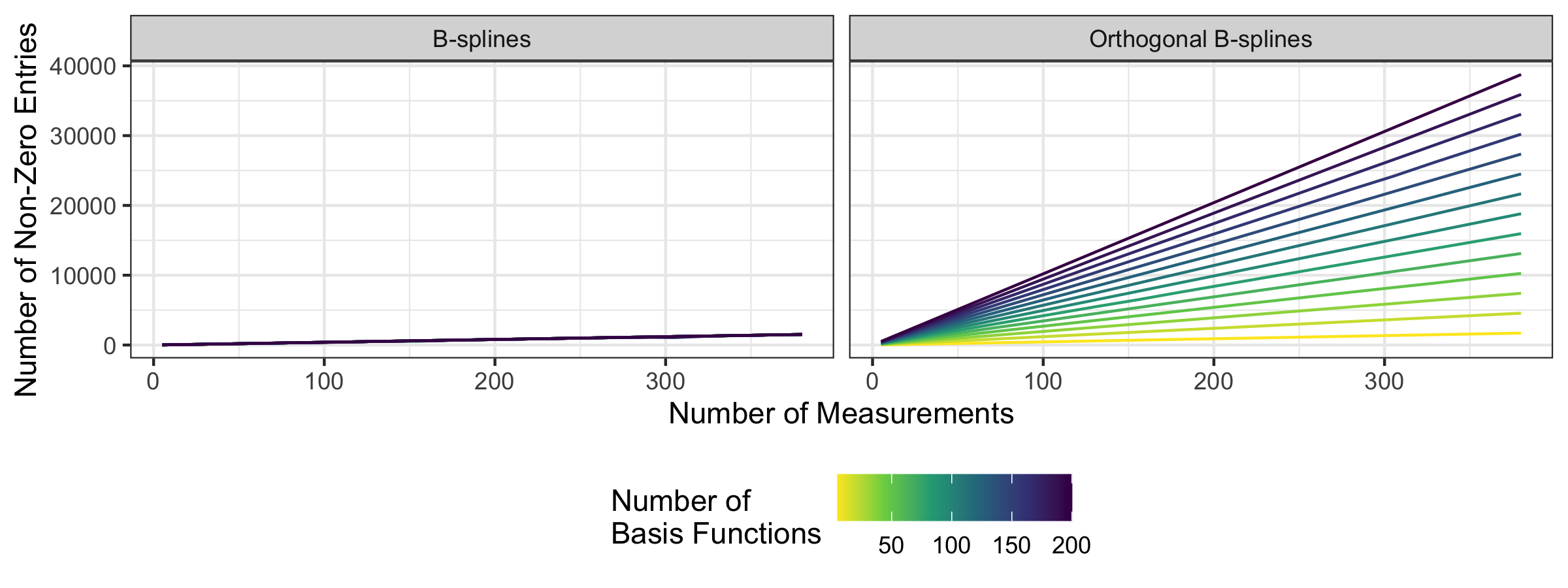
Figure S1: Number of non-zero entries in a B-spline matrix with $n_{i}$ uniformly spaced observations and $P$ basis functions based on uniformly-spaced knots.

The complete orthonormalization step then consists of orthonormalizing separately $\Theta_{g,\mathcal{X}}$ and $\Theta_{g,\mathcal{Y}}$ for each $g$ as described above and as in Zhou et al., (2008), while also adjusting $\Lambda_{g}$ appropriately.

S6 Additional Simulation Plots and Results

We give further plots on our simulation studies, beginning with the first simulation. To further describe the setup of this simulation, in Figure S2, we plot the true principal components used for the first simulation.

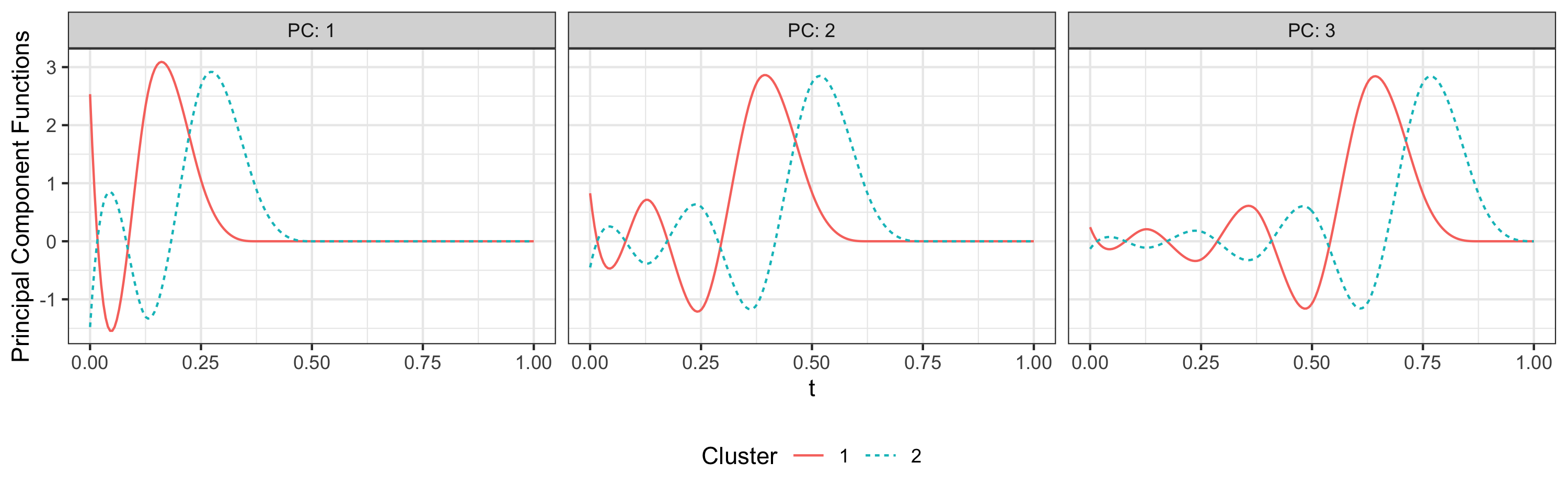
Figure S2: Principal component functions in the first simulation. The $\ell$-th PC of the $g$-th group is the $(g+2\ell)$-th function of an orthogonal spline basis with dimension $11$ with uniformly space knots.

In Figure S3, we plot the effective sample size using importance sampling for the first simulation, as well as the adjusted Rand index (ARI). Overall, we see healthy adaptation in the importance sample weights, providing helpful variability in the MCEM algorithm. In this figure, we also demonstrate that the adjusted Rand index (ARI) used in Liang et al., (2020) displays similar clustering results when comparing the different estimation strategies.

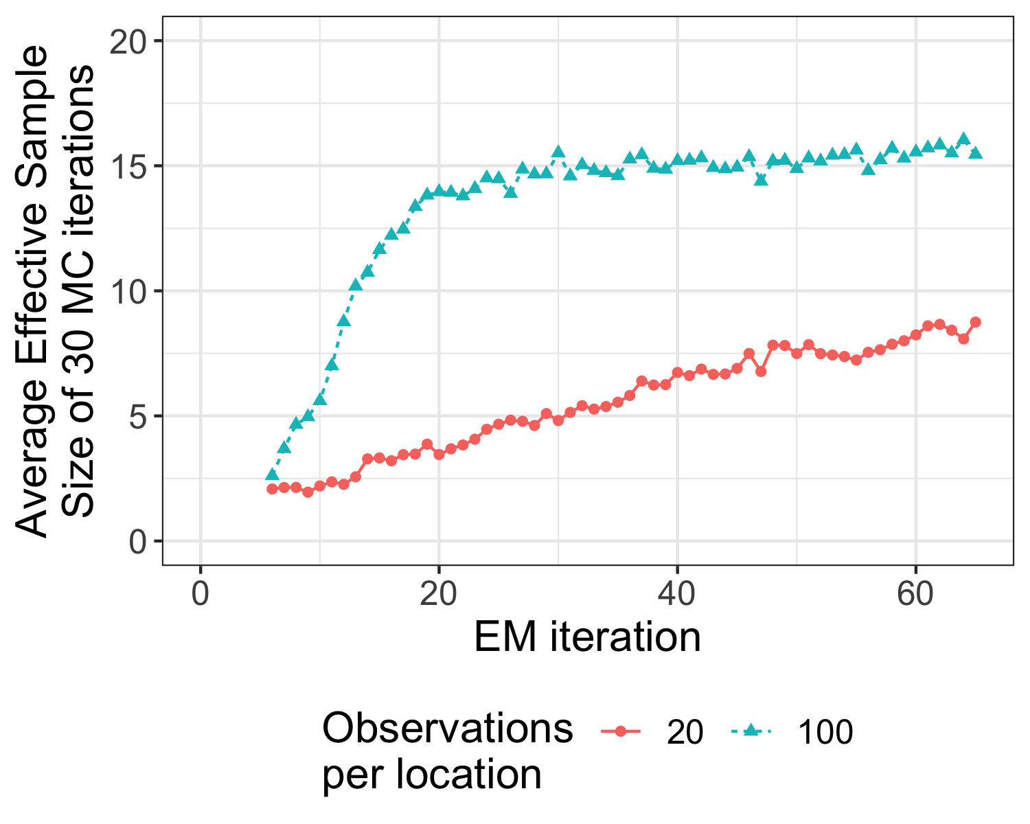
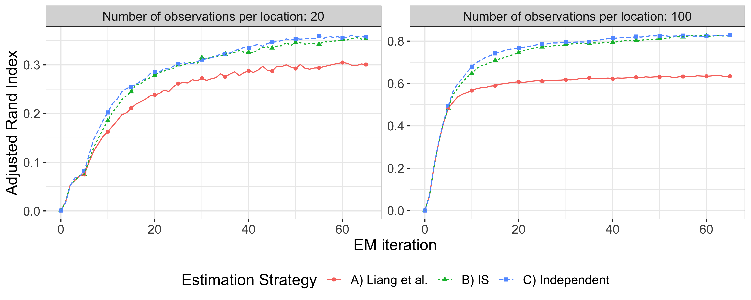
Figure S3: (Left) Average effective sample size (ESS) for importance sampling in the first simulation for each EM iteration. (Right) We plot the adjusted Rand index (ARI) used in Liang et al., (2020).

Turning now to the second simulation study, in Figure S4, we plot other principal component and linear transformation functions. In Table 3, we display the estimation results for marginal variance and range scale parameters for the principal component random fields of the predictor random field $\mathcal{X}$.

Figure S4: Additional function approximation results from the simulation study. Shaded region corresponds to 2 pointwise empirical standard deviations from the mean. From left to right: The third principal component function $\phi_{3}$ and then $\mathscr{F}\psi_{2}$ and $\mathscr{F}\psi_{3}$

$\ell$	$\sigma^{2}_{\alpha,\ell}$	$\hat{\sigma}^{2}_{\alpha,\ell}$	$\kappa_{\alpha,\ell}$	$\hat{\kappa}_{\alpha,\ell}$	$\sigma_{\alpha,\ell}^{2}/\kappa_{\alpha,\ell}$	$\hat{\sigma}^{2}_{\alpha,\ell}/\hat{\kappa}_{\alpha,\ell}$
1	$1.30$	1.28 (0.13)	$0.05$	0.05 (0.01)	$26$	26.46 (2.06)
2	$0.50$	0.49 (0.05)	$0.06$	0.06 (0.01)	$8.33$	8.37 (0.74)
3	$0.20$	0.20 (0.02)	$0.05$	0.05 (0.01)	$4.00$	4.05 (0.34)
4	$0.10$	0.10 (0.01)	$0.06$	0.06 (0.01)	$1.67$	1.68 (0.13)

Table 3: True and estimated parameters of the random fields of principal component scores for the predictor random field $\mathcal{X}$. Numbers in brackets denote 1 empirical standard error based on 100 independent simulations.

S7 Data Description

We described the data used in the analysis here. We use:

• the May 5, 2021 high-resolution MLR snapshot of the SOCCOM data:
  http://doi.org/10.6075/J0T43SZG (Johnson et al.,, 2020),

• the June 6, 2021 snapshot of the Argo data for nearby core data:
  http://doi.org/10.17882/42182#85023 (Argo,, 2020).

For the SOCCOM data, we remove measurements with: a) salinity less than $28$ practical salinity units (PSU), b) latitude greater than $-25$ degrees, c) pressure less than $0$ or greater than $2{,}000$, d) oxygen quality control denotes “bad” (8) e) temperature, salinity, or pressure quality control is not good (0) f) missing pressure or location data (this keeps linearly interpolated locations while under ice part of the data).

Following these reductions, we remove profiles with

• any measurements of salinity less than $33$ PSU or greater than $37.2$ PSU

• a pressure gap of $200$ decibars or more between consecutive measurements

• a minimum pressure greater than $100$ decibars or a maximum pressure less than $1{,}450$ decibars

• fewer than 15 measurements

• had a potential density estimated derivative less than $-0.05$ kg/L/decibar

• there are fewer than five oxygen measurements with good (0) or probably good (4) quality control

• an oxygen measurement greater than $400\ \mu$mol/kg

Finally, for the response, we only consider data with good (0) or probably good (4) quality control.

For Core Argo data with temperature and salinity only, we make similar, but not identical, exclusions for profiles (note that the Argo and SOCCOM data have different quality flag meanings):

• any measurements of salinity less than $33$ PSU or greater than $37.2$ PSU

• a pressure gap of $200$ decibars or more between consecutive measurements

• a minimum pressure greater than $100$ decibars or a maximum pressure less than $1{,}450$ decibars

• temperature, salinity, or pressure quality control is not good (3, 4)

• missing pressure or location data (this keeps linearly interpolated locations while under ice part of the data)

• the pressure adjusted error was greater than $16$ decibars

• the closest SOCCOM profile was greater than $500$ kilometers away

Observations were also removed with pressure less than $0$ decibar or greater than $2{,}000$ decibars.

S8 Details for the Initialization

Here we provide more details on the initialization procedure. First, we run $k$-means for interpolated values of the data to obtain an initial cluster assignment. After this initialization, we use the model introduced in Zhou et al., (2008) and extend it to a Gaussian mixture model. Let $\boldsymbol{Y}_{i}$ and $\boldsymbol{X}_{i}$ be defined as in the main document, and let $\mathcal{Y}_{1},\dots,\mathcal{Y}_{n}$ and $\mathcal{X}_{1},\dots,\mathcal{X}_{n}$ be the underlying functional random variables at each location. We now assume that the pairs $(\mathcal{X}_{i},\mathcal{Y}_{i})$ are $n$ i.i.d. functional random variables. Furthermore, we have the unobserved i.i.d. latent variables $Z_{1},\dots,Z_{n}$ uniformly distributed on $\{1,\dots,G\}$. We assume that the $\mathcal{Y}_{i}$ admit the eigendecompositions

$$\mathcal{Y}_{i}=\mu_{Z_{i},\mathcal{Y}}+\sum_{\ell=1}^{Q_{1}}\beta_{i\ell}\phi_{Z_{i},\ell}.$$

and the random variables $\mathcal{X}_{i}$ admit the eigendecompositions

$$\mathcal{X}_{i}=\mu_{Z_{i},\mathcal{X}}+\sum_{\ell=1}^{Q_{1}}\alpha_{i\ell}\psi_{Z_{i},\ell},$$

so that

$$Y(s_{i},t_{ij}) =\mu_{Z_{i},\mathcal{Y}}(t_{ij})+\sum_{\ell=1}^{Q_{1}}\beta_{i\ell}\phi_{Z_{i},\ell}(t_{ij})+\epsilon_{ij}^{Y}$$

$$X(s_{i},t_{ij}) =\mu_{Z_{i},\mathcal{X}}(t_{ij})+\sum_{\ell=1}^{Q_{1}}\alpha_{i\ell}\psi_{Z_{i},\ell}(t_{ij})+(\epsilon^{X_{1}}_{i1},\dots,\epsilon^{X_{K}}_{iK}),$$

where the $\{\epsilon_{il}\}$ are i.i.d. mean zero Gaussian random variables with variance $\tilde{\sigma}_{Y}^{2}$, and the $\epsilon^{X_{k}}$ are i.i.d. Gaussian random vectors with independent components whose marginal variances are $\tilde{\sigma}_{X_{k}}^{2}$. Let $\boldsymbol{\alpha}_{i}=(\alpha_{i1},\dots,\alpha_{iQ_{1}})$ and $\boldsymbol{\beta}_{i}=(\beta_{i1},\dots,\beta_{iQ_{1}})$. Furthermore, let $\Sigma_{Z_{i},\alpha}=\mathbb{V}\textrm{ar}(\boldsymbol{\alpha}_{i}|Z_{i})$ and $\Sigma_{Z_{i},\beta}=\mathbb{V}\textrm{ar}(\boldsymbol{\beta}_{i}|Z_{i})$. To model the correlation between $\mathcal{X}_{i}$ and $\mathcal{Y}_{i}$, we use a linear regression model for the principal component scores, that is

$$\left(\begin{matrix}\boldsymbol{\beta}_{i}\\ \boldsymbol{\alpha}_{i}\end{matrix}\middle|Z_{i}\right)\sim\mathcal{N}\left(0,\begin{pmatrix}\Sigma_{Z_{i},\beta}&C_{Z_{i}}\Sigma_{Z_{i},\alpha}\\ \Sigma_{Z_{i},\alpha}C_{Z_{i}}^{\top}&\Sigma_{Z_{i},\alpha}\end{pmatrix}\right).$$

Using the similar notation as in the main document, we approximate

$$(I_{K}\otimes B(t))\tilde{\Theta}_{\mathcal{X}} \approx(\psi_{1}(t),\dots,\psi_{Q_{1}}(t))$$

$$(I_{K}\otimes B(t))\tilde{\theta}_{g,\mathcal{X}} \approx\mu_{g,\mathcal{X}}(t)$$

$$B(t)\tilde{\Theta}_{\mathcal{Y}} \approx(\phi_{1}(t),\dots,\phi_{Q_{1}}(t))$$

$$B(t)\tilde{\theta}_{g,\mathcal{Y}} \approx\mu_{g,\mathcal{Y}}(t)$$

The parameters are then estimated similarly to the procedure in the main document, with the only change being that the MCEM procedure is simpler as all spatial correlation is ignored so that obtaining the samples $\left\{\boldsymbol{\alpha}^{(\tau)}_{i},\boldsymbol{\beta}_{i}^{(\tau)},Z_{i}^{(\tau)}\right\}_{i=1}^{n}$ for $\tau=1,\dots,n$ is straightforward. Most M-step updates are analogous to the ones outlined in Section S4, and the M-step updates for $\{\Sigma_{g,\alpha}\}$, $\{\Sigma_{g,\beta}\}$ and $\{C_{g}\}_{g=1}^{G}$ can be found in Zhou et al., (2008).

After estimating the above model by running the MCEM algorithm for a few iterations, we initialize as follows

$$\theta_{g,\mathcal{X}} =\tilde{\theta}_{g,\mathcal{X}}$$

$$\theta_{g,\mathcal{Y}} =\tilde{\theta}_{g,\mathcal{Y}}$$

$$\Theta_{g,\mathcal{X}} =\tilde{\Theta}_{g,\mathcal{X}}$$

$$\Lambda_{g} =\tilde{\Theta}_{g,\mathcal{Y}}C_{g}$$

$$\sigma_{Y}^{2} =\tilde{\sigma}_{Y}^{2}$$

$$\sigma_{X_{k}}^{2} =\tilde{\sigma}_{X_{k}}^{2},~{}~{}~{}k=1,\dots,K.$$

Then, we compute the residuals based on this model based on the last MC iteration. That is we compute

$$\tilde{E}(s_{i},t_{ij})=Y(s_{i},t_{ij})-B(t_{ij})\theta_{Z_{i}^{(T)},\mathcal{Y}}-B(t_{ij})\Lambda_{Z_{i}^{(T)}}\boldsymbol{\alpha}_{i}^{(T)},$$

and assume that there exist functions $\varphi_{1},\dots,\varphi_{Q_{2}}$ and independent random fields

$$\left\{\left\{\eta_{g,\ell}(s)\right\}_{\ell=1}^{Q_{2}}\right\}_{g=1}^{G}$$

such that

$$\tilde{E}(s_{i},t_{ij})=\sum_{\ell=1}^{Q_{2}}\eta_{Z_{i}^{(T)},\ell}(s_{i})\varphi_{Z_{i}^{(T)},\ell}(t_{ij})+\tilde{\epsilon}_{ij}.$$

Again, we approximate

$$B(t)\tilde{\Theta}_{g,\mathcal{E}}=(\varphi_{1}(t),\dots,\varphi_{Q_{2}}(t)).$$

We then run a single M-step update for $\tilde{\Theta}_{g,\mathcal{E}}$ and initialize $\Theta_{g,\mathcal{E}}=\tilde{\Theta}_{g,\mathcal{E}}$.

S9 Description of Prediction Formulas

As in other parts of the supplement, we ignore the dependence on clusters in the following developments. In Proposition 1 and Section S2, we found that, in each cluster,

$$\boldsymbol{\alpha},\boldsymbol{\eta}|\boldsymbol{X},\boldsymbol{Y}\sim\mathcal{N}\left((A^{-1}+U^{\top}U)^{-1}U^{\top}\begin{pmatrix}\boldsymbol{X}_{0}\\ \boldsymbol{Y}_{0}\end{pmatrix},(A^{-1}+U^{\top}U)^{-1}\right)$$

where $\boldsymbol{X}_{0}$ and $\boldsymbol{Y}_{0}$ are centered versions of the data, $A=\begin{pmatrix}\Sigma_{\alpha}&0\\ 0&\Sigma_{\eta}\end{pmatrix}$, and $U$ defined in Section S2.

We now consider new scores $\check{\boldsymbol{\alpha}}$ and $\check{\boldsymbol{\eta}}$ where we want to predict, potentially with additional predictor data $\check{\boldsymbol{X}}$. For simplicity, suppose that $\check{\boldsymbol{X}}$ is available; however, we discuss later how to form predictions when $\check{\boldsymbol{X}}$ is not available. Consider the matrix

$$\check{A} =\begin{pmatrix}\Sigma_{\alpha}&\Sigma_{\alpha,\check{\alpha}}&0&0\\ \Sigma_{\alpha,\check{\alpha}}^{\top}&\Sigma_{\check{\alpha}}&0&0\\ 0&0&\Sigma_{\eta}&\Sigma_{\eta,\check{\eta}}\\ 0&0&\Sigma_{\eta,\check{\eta}}^{\top}&\Sigma_{\check{\eta}}\end{pmatrix}$$

where $\Sigma_{\alpha,\check{\alpha}}=\mathbb{C}\textrm{ov}(\boldsymbol{\alpha},\check{\boldsymbol{\alpha}})$, $\Sigma_{\check{\alpha}}=\mathbb{V}\textrm{ar}(\check{\boldsymbol{\alpha}})$, and likewise for the other matrices involving $\eta$. Also, note that $\check{A}^{-1}$ can be formed using a Vecchia approximation for the entire matrix $\begin{pmatrix}\Sigma_{\alpha}&\Sigma_{\alpha,\check{\alpha}}\\ \Sigma_{\alpha,\check{\alpha}}^{\top}&\Sigma_{\check{\alpha}}\end{pmatrix}^{-1}$ and likewise for $\eta$ and $\check{\eta}$.

Recall the definition of $U$ in Section S2, and similarly define the matrices

$$U_{X,\alpha} =D_{X}^{-1/2}\boldsymbol{B}\Theta_{\mathcal{X}}$$

$$U_{Y,\alpha} =\sigma_{Y}^{-1}\tilde{\boldsymbol{B}}\Lambda$$

$$U_{Y,\eta} =\sigma_{Y}^{-1}\tilde{\boldsymbol{B}}\Theta_{\mathcal{Y}}$$

so that $U=\begin{pmatrix}U_{X,\alpha}&0\\ U_{Y,\alpha}&U_{Y,\eta}\end{pmatrix}$. Furthermore, let

$$U_{\textrm{all}} =\begin{pmatrix}U_{X,\alpha}&0&0&0\\ U_{Y,\alpha}&0&U_{Y,\eta}&0\\ 0&U_{\check{X},\check{\alpha}}&0&0\end{pmatrix}$$

where $U_{\check{X},\check{\alpha}}=D_{\check{X}}^{-1/2}\boldsymbol{B}_{\check{X}}\Theta_{\mathcal{X}}$ is the respective matrix for the new data. The three groups of rows correspond to $\boldsymbol{X}$ and $\boldsymbol{Y}$, and $\check{\boldsymbol{X}}$, respectively, while the four groups of columns correspond to $\boldsymbol{\alpha}$, $\check{\boldsymbol{\alpha}}$, $\boldsymbol{\eta}$, and $\check{\boldsymbol{\eta}}$.

Proposition 3.

In this case, the conditional distribution of the scores can be written:

$$\boldsymbol{\alpha},\check{\boldsymbol{\alpha}},\boldsymbol{\eta},\check{\boldsymbol{\eta}}|\boldsymbol{X},\boldsymbol{Y},\check{\boldsymbol{X}}\sim\mathcal{N}\left(\left(\check{A}^{-1}+U_{\textrm{all}}^{\top}U_{\textrm{all}}\right)^{-1}U_{\textrm{all}}^{\top}\begin{pmatrix}{\boldsymbol{X}_{0}}\\ {\boldsymbol{Y}}_{0}\\ \check{{\boldsymbol{X}}}_{0}\end{pmatrix},\left(\check{A}^{-1}+U_{\textrm{all}}^{\top}U_{\textrm{all}}\right)^{-1}\right)$$

where ${\boldsymbol{X}}_{0}$, ${\boldsymbol{Y}}_{0}$, and $\check{{\boldsymbol{X}}}_{0}$ are centered versions of the data.

Proof of Proposition 3.

We sketch the proof, which is similar to that of Proposition 2. Define $D_{\check{X}}$ analogously to $D_{X}$ and $\check{\boldsymbol{B}}$ to be the basis matrix for $\check{\boldsymbol{X}}$. Furthermore, define $\boldsymbol{\alpha}_{a}=\begin{pmatrix}\boldsymbol{\alpha}\\ \check{\boldsymbol{\alpha}}\end{pmatrix}$ and $\Sigma_{\alpha_{a}}=\mathbb{V}\textrm{ar}(\boldsymbol{\alpha}_{a})=\begin{pmatrix}\Sigma_{\alpha}&\Sigma_{\alpha,\check{\alpha}}\\ \Sigma_{\alpha,\check{\alpha}}^{\top}&\Sigma_{\check{\alpha}}\end{pmatrix}$ and likewise for $\boldsymbol{\eta}_{a}$ and $\Sigma_{\eta_{a}}$. Following the same approach as in Proposition 2, we have

$$f {}_{\boldsymbol{\alpha}_{a},\boldsymbol{\eta}_{a}|\boldsymbol{X},\boldsymbol{Y},\check{\boldsymbol{X}}}(\boldsymbol{\alpha}_{a},\boldsymbol{\eta}_{a})\propto f_{\boldsymbol{X}|\boldsymbol{\alpha}}(\mathbf{X})f_{\boldsymbol{Y}|\boldsymbol{\alpha},\boldsymbol{\eta}}(\boldsymbol{Y})f_{\check{\boldsymbol{X}}|\check{\boldsymbol{\alpha}}}(\check{\boldsymbol{X}})f_{\boldsymbol{\alpha}_{a}}(\boldsymbol{\alpha}_{a})f_{\boldsymbol{\eta}_{a}}(\boldsymbol{\eta}_{a})$$

$$\propto\exp\left(-\frac{1}{2}\sum_{i=1}^{n}(\boldsymbol{X}_{i}-\boldsymbol{B}_{i}(\theta_{\mathcal{X}}+\Theta_{\mathcal{X}}\boldsymbol{\alpha}_{i}))^{\top}D_{X^{i}}^{-1}(\boldsymbol{X}_{i}-\boldsymbol{B}_{i}(\theta_{\mathcal{X}}+\Theta_{\mathcal{X}}\boldsymbol{\alpha}_{i}))\right)$$

$$~{}~{}~{}~{}\times\exp\left(-\frac{1}{2\sigma_{Y}^{2}}\sum_{i=1}^{n}\left\lVert\boldsymbol{Y}_{i}-B_{i}(\theta_{\mathcal{Y}}+\Lambda\boldsymbol{\alpha}_{i}+\Theta_{\mathcal{E}}\boldsymbol{\eta}_{i})\right\rVert^{2}\right)$$

$$~{}~{}~{}~{}\times\textrm{exp}\left(-\frac{1}{2}(\check{\boldsymbol{X}}-\check{\boldsymbol{B}}(\theta_{\mathcal{X}}+\Theta_{\mathcal{X}}\check{\boldsymbol{\alpha}}))^{\top}D_{\check{X}}^{-1}(\check{\boldsymbol{X}}-\check{\boldsymbol{B}}(\theta_{\mathcal{X}}+\Theta_{\mathcal{X}}\check{\boldsymbol{\alpha}}))\right)$$

$$~{}~{}~{}~{}\times\exp\left(-\frac{1}{2}\boldsymbol{\eta}_{a}^{\top}\Sigma_{\eta_{a}}^{-1}\boldsymbol{\eta_{a}}\right)\times\exp\left(-\frac{1}{2}\boldsymbol{\alpha}_{a}^{\top}\Sigma_{\alpha_{a}}^{-1}\boldsymbol{\alpha}_{a}\right)$$

$$\propto\exp\left(-\frac{1}{2}\begin{pmatrix}\boldsymbol{\alpha}_{a}\\ \boldsymbol{\eta}_{a}\end{pmatrix}^{\top}\Sigma_{a}^{-1}\begin{pmatrix}\boldsymbol{\alpha}_{a}\\ \boldsymbol{\eta}_{a}\end{pmatrix}\right)$$

$$~{}~{}~{}~{}\times\exp\left(\boldsymbol{\alpha}^{\top}\left[D_{X}^{-1}(\boldsymbol{B}\Theta_{\mathcal{X}})^{\top}(\boldsymbol{B}\theta_{\mathcal{X}}-\boldsymbol{X})+\sigma_{Y}^{-2}(\tilde{\boldsymbol{B}}\Lambda)^{\top}(\tilde{\boldsymbol{B}}\theta_{\mathcal{Y}}-\boldsymbol{Y})\right]\right)$$

$$~{}~{}~{}~{}\times\exp\left(\boldsymbol{\eta}^{\top}\left[\sigma_{Y}^{-2}(\tilde{\boldsymbol{B}}\Theta_{\mathcal{E}})^{\top}(\tilde{\boldsymbol{B}}\theta_{\mathcal{Y}}-\boldsymbol{Y})\right]\right)\exp\left(\check{\boldsymbol{\alpha}}^{\top}\left[D_{\check{X}}^{-1}(\check{\boldsymbol{B}}\Theta_{\mathcal{X}})^{\top}(\check{\boldsymbol{B}}\theta_{\mathcal{X}}-\check{\boldsymbol{X}})\right]\right)$$

where

$$\Sigma_{a}^{-1} =\begin{pmatrix}\Sigma_{\alpha_{a}}^{-1}+\begin{pmatrix}U_{X,\alpha}^{\top}U_{X,\alpha}+U_{Y,\alpha}^{\top}U_{Y,\alpha}&0\\ 0&U_{\check{X},\check{\alpha}}^{\top}U_{\check{X},\check{\alpha}}\end{pmatrix}&\begin{pmatrix}U_{Y,\alpha}^{\top}U_{Y,\eta}&0\\ 0&0\end{pmatrix}\\ \begin{pmatrix}U_{Y,\alpha}^{\top}U_{Y,\eta}&0\\ 0&0\end{pmatrix}&\Sigma_{\eta_{a}}^{-1}+\begin{pmatrix}U_{Y,\eta}^{\top}U_{Y,\eta}&0\\ 0&0\end{pmatrix}\end{pmatrix}$$

$$=\check{A}^{-1}+U_{\textrm{all}}^{\top}U_{\textrm{all}}.$$

Each entry of $0$ added to the matrix represents the scores at the new location. This gives the conditional covariance matrix $\Sigma_{a}$, and following the steps of the proof of Proposition 2 directly gives the conditional mean as well. ∎

This shows that prediction is quite similar to the computations in the E-step. Likewise, when $\check{\boldsymbol{X}}$ is not available, we form $U_{\textrm{all}}$ with one group of rows deleted:

$$U_{\textrm{all}} =\begin{pmatrix}U_{X,\alpha}&0&0&0\\ U_{Y,\alpha}&0&U_{Y,\eta}&0\end{pmatrix}$$

and compute the same formulas with only $\boldsymbol{X}$ and $\boldsymbol{Y}$ as the available data.

S10 Product

The predicted clusters, oxygen, temperature, and salinity values, as well as their uncertainties, are given and described in the Google Drive folder https://drive.google.com/drive/folders/1_rG5woV45UHsLpX7sWl3C-lWRaNvZysX?usp=sharing.

In Figure S5, we plot the predicted clusters for each of the 12 months.

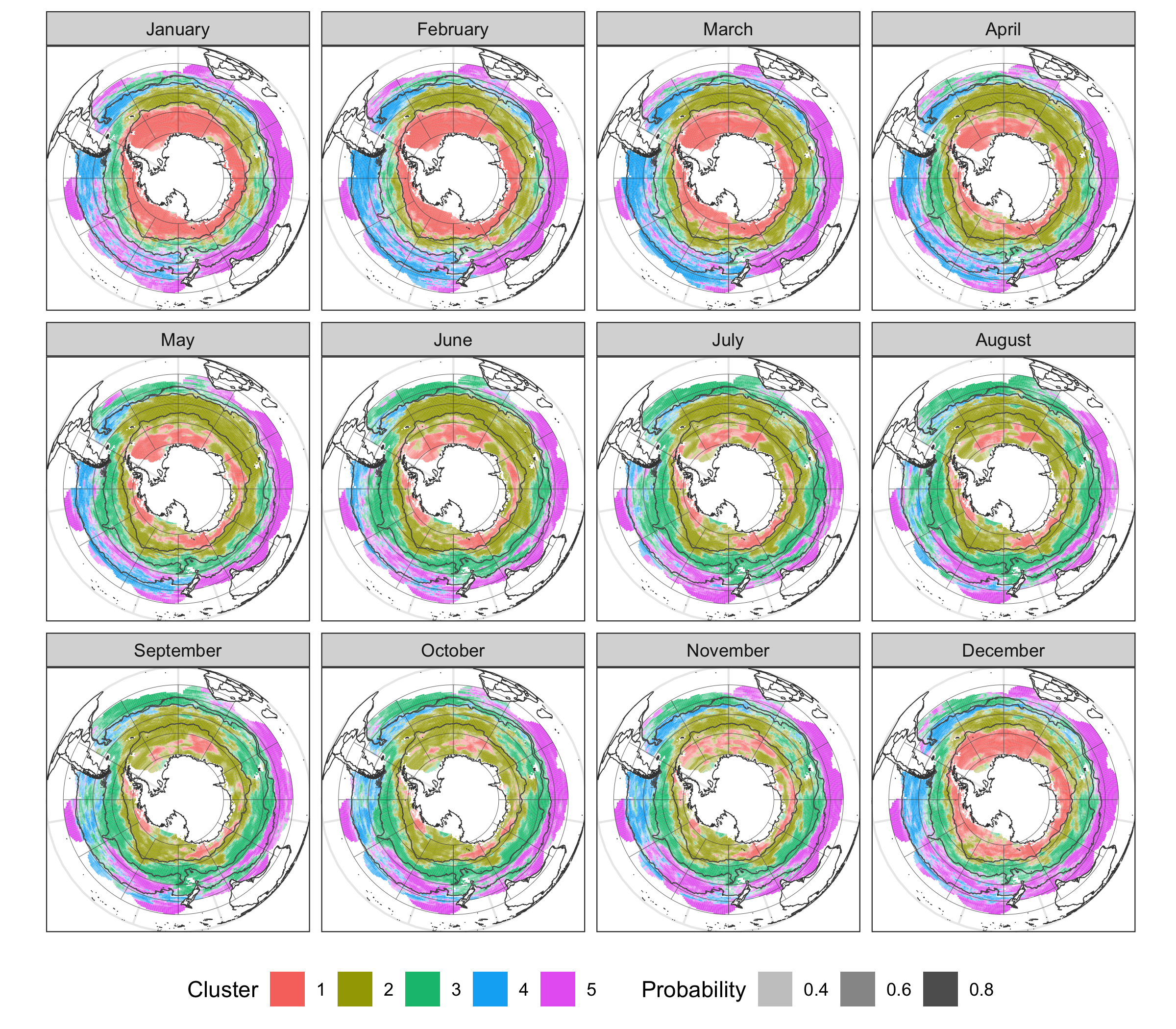
Figure S5: Cluster membership information for each month of the year.

S11 Additional Data Analysis Plots

We show additional data analysis plots of interest in a variety of figures. In Figure S6, we plot our AIC-based model selection criterion for different number of principal components. In Figures S7 and S8, we demonstrate the seasonality dependence of the cluster memberships, showing fairly different clusters for January versus July. In Figures S9, S10, and S11, we plot predictions, predictive variances, and means for temperature and salinity, respectively, which are obtained naturally from our analysis of temperature, salinity, and oxygen. Similarly, we plot the first principal component of each estimated in Figure S12: principal components of temperature and salinity, linear transformation functions, and principal components for $\mathcal{E}$. In Figure S13, we break down the oxygen variability by the cluster. We plot the length of uncertainty estimates in Figure S14 in the leave-out experiments, showing that, as expected, predicted uncertainties for leave-float-out are higher than for leave-profile-out. In Figure S15, we give an account of the proportion of variance explained in oxygen by location, and in Figure S16 we consider the two contributions to the oxygen uncertainty in (10) and (11). In Figure S16 we can identify areas where the cluster membership is uncertain. In Figure S17, we plot predicted functions over varying latitude with fixed longitude. In Figure S18, we plot the estimated log-likelihood (as calculated in Section 3.4), as a function of the EM iteration, showing that our estimation strategy estimates parameters that increase the log-likelihood. In Figure S19, we plot predictions and variances for nitrate.

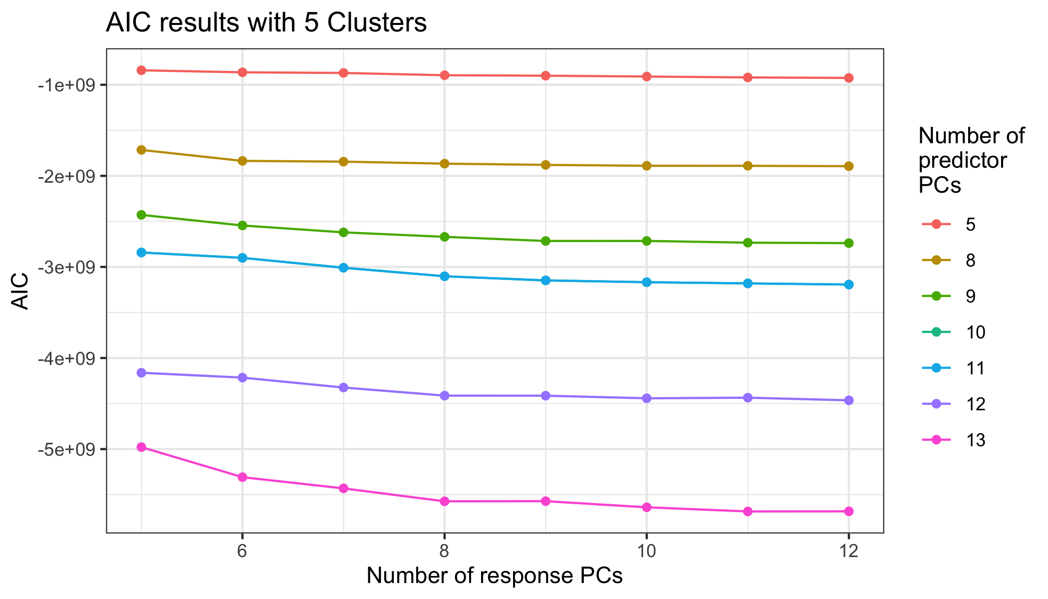
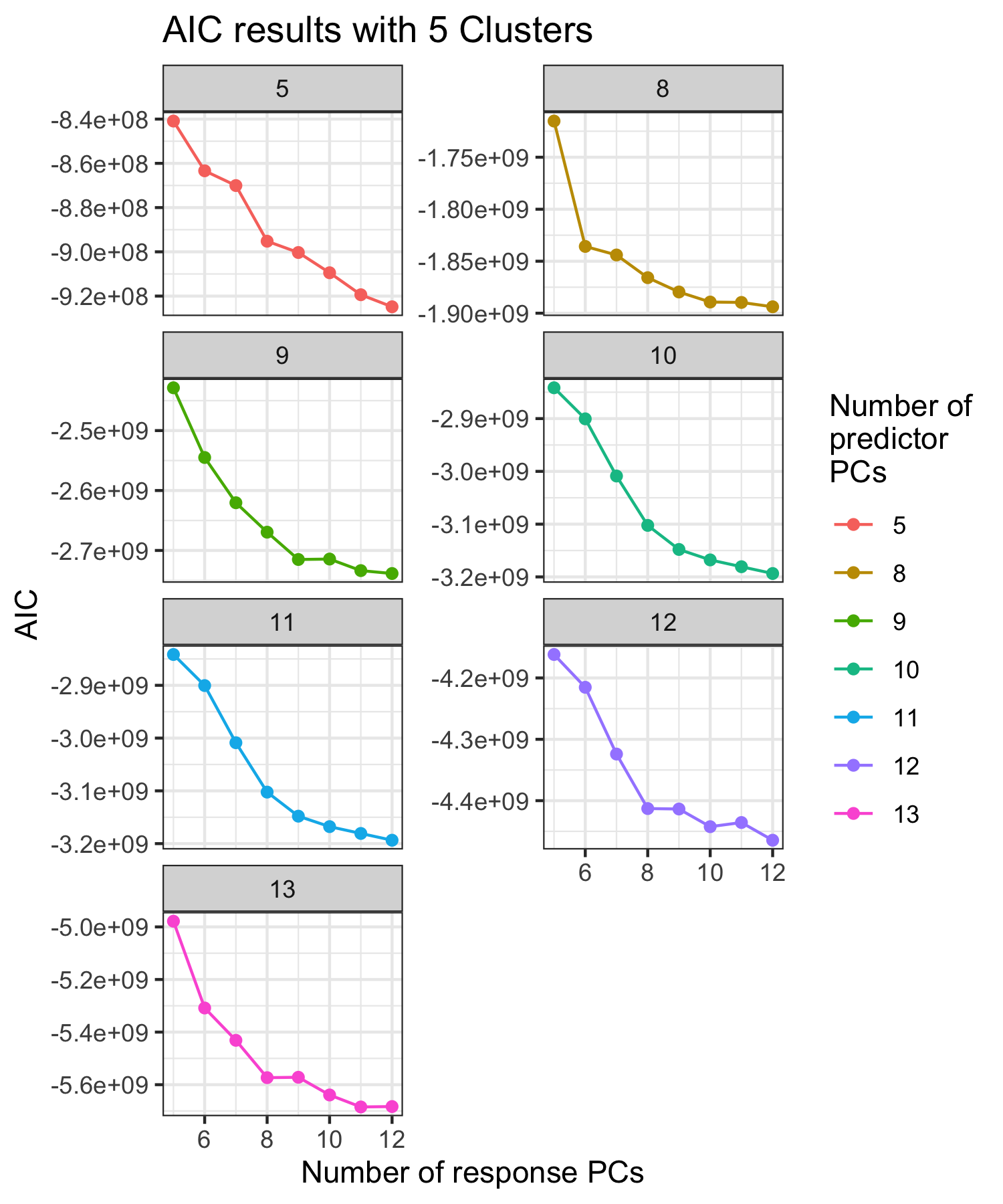
Figure S6: Akaike Information Criterion values for varying number of principal components for the covariates and the response. In general, the AIC seems to be decreasing as a function of both principal components, though it increases from 12 to 13 response PCs.

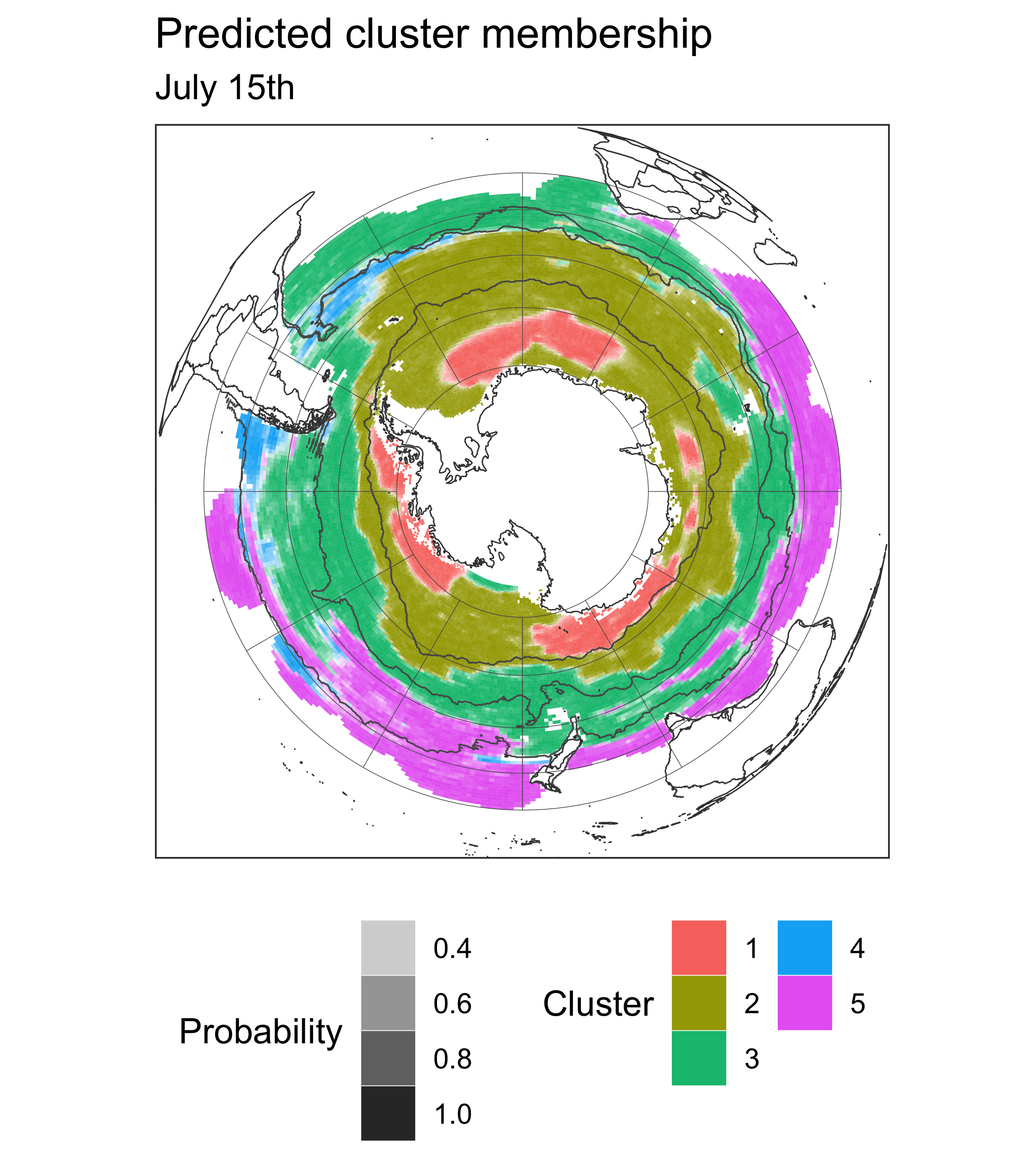
Figure S7: Marginal membership information for January (left, summer) and July (right, winter). This demonstrates seasonal differences in oceanographic fronts.

Figure S8: Cluster membership of BGC Argo profiles, in a histogram summarized by the day of the year (seasonality).

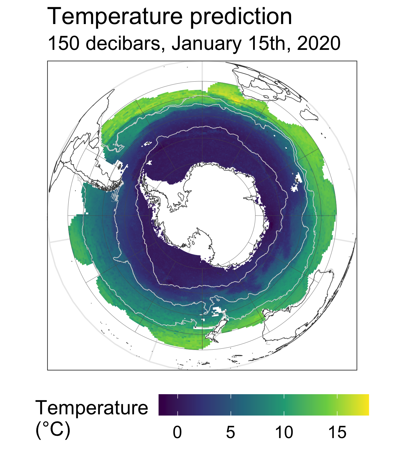
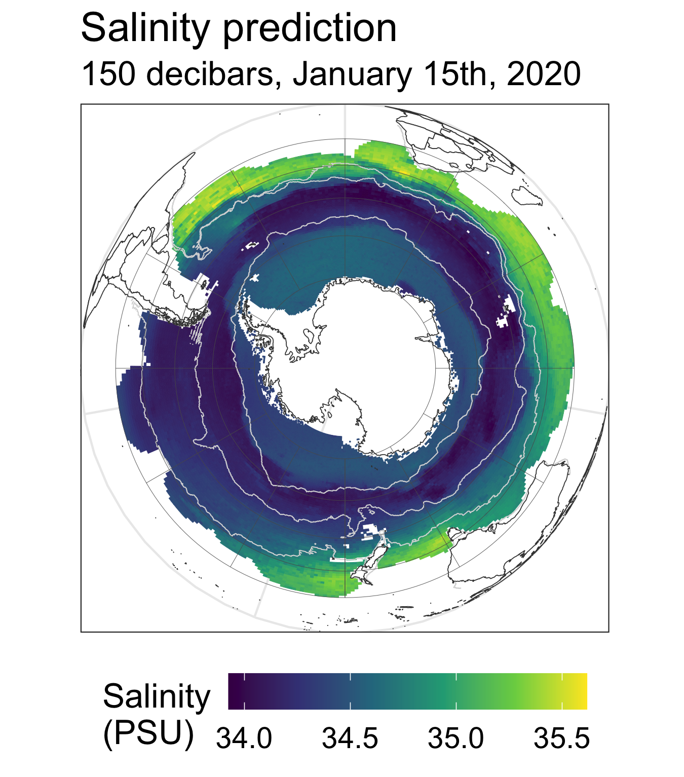
Figure S9: Temperature (left) and salinity (right) predictions for January 15th, 2020 at 150 decibar.

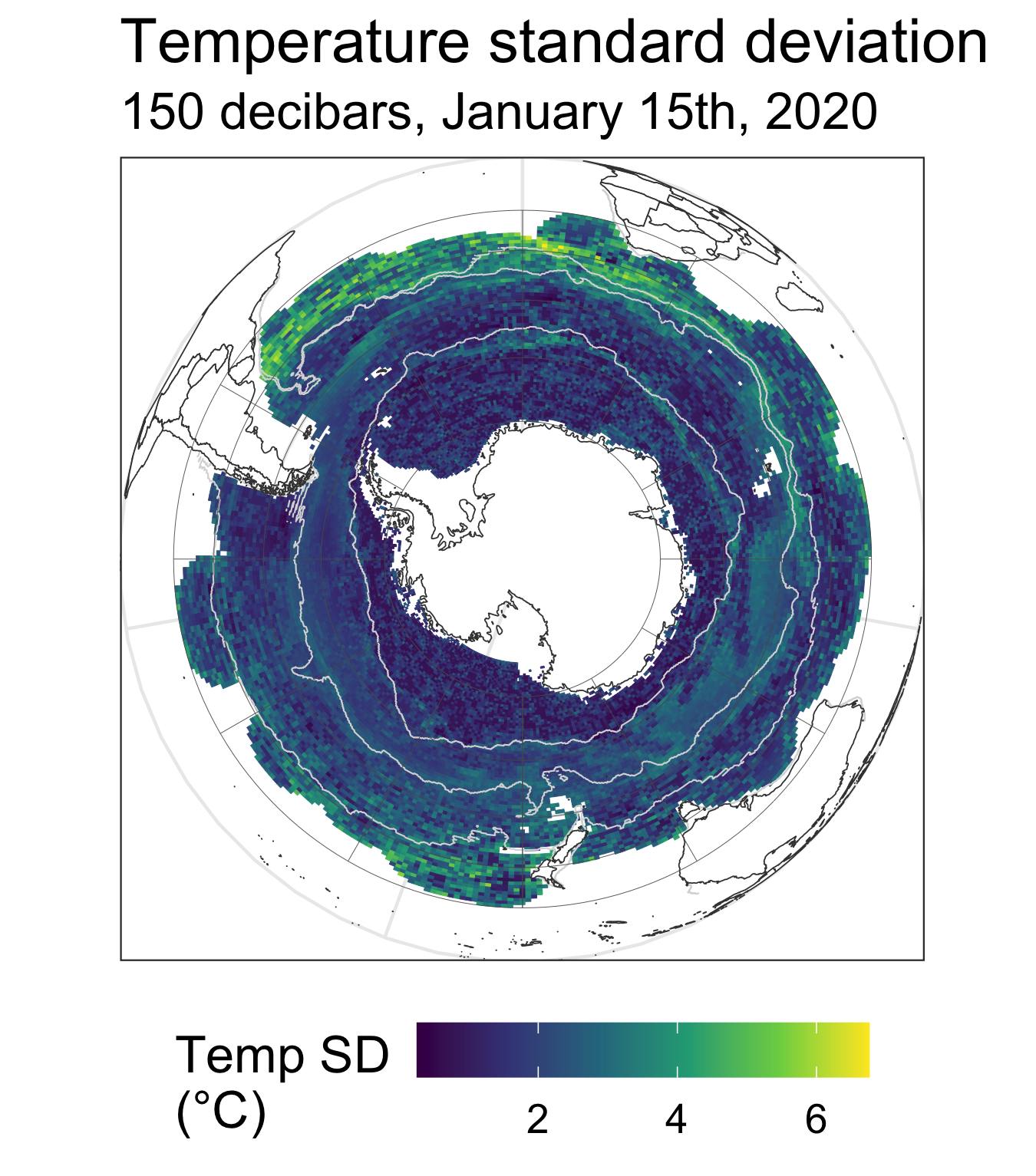
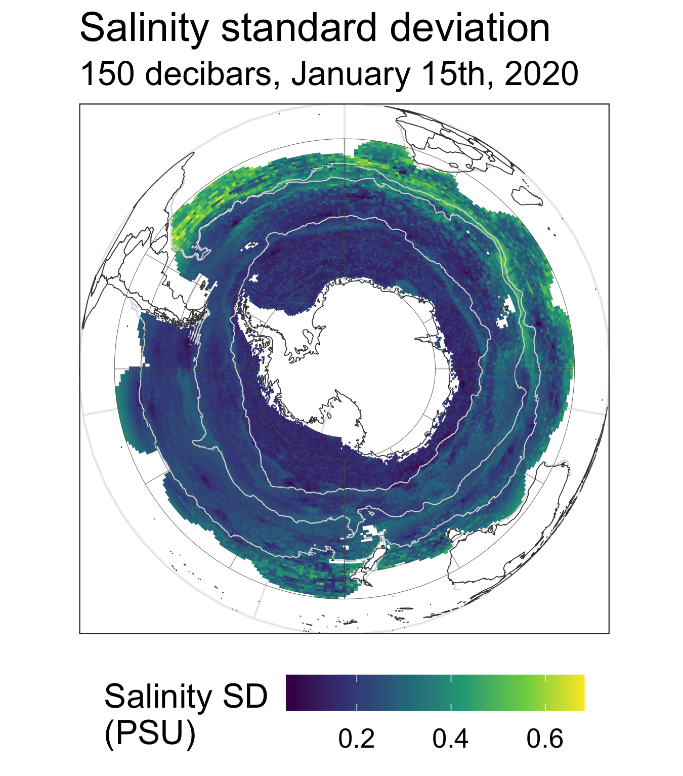
Figure S10: Temperature (left) and salinity (right) predicted standard deviations for January 15th, 2020 at 150 decibar.

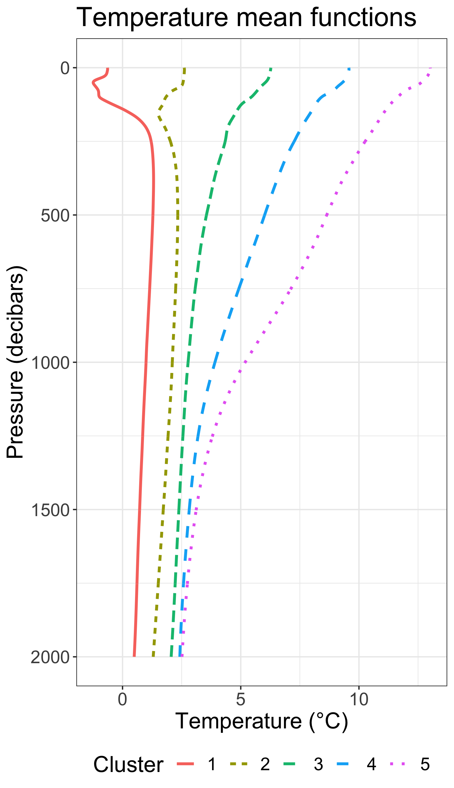
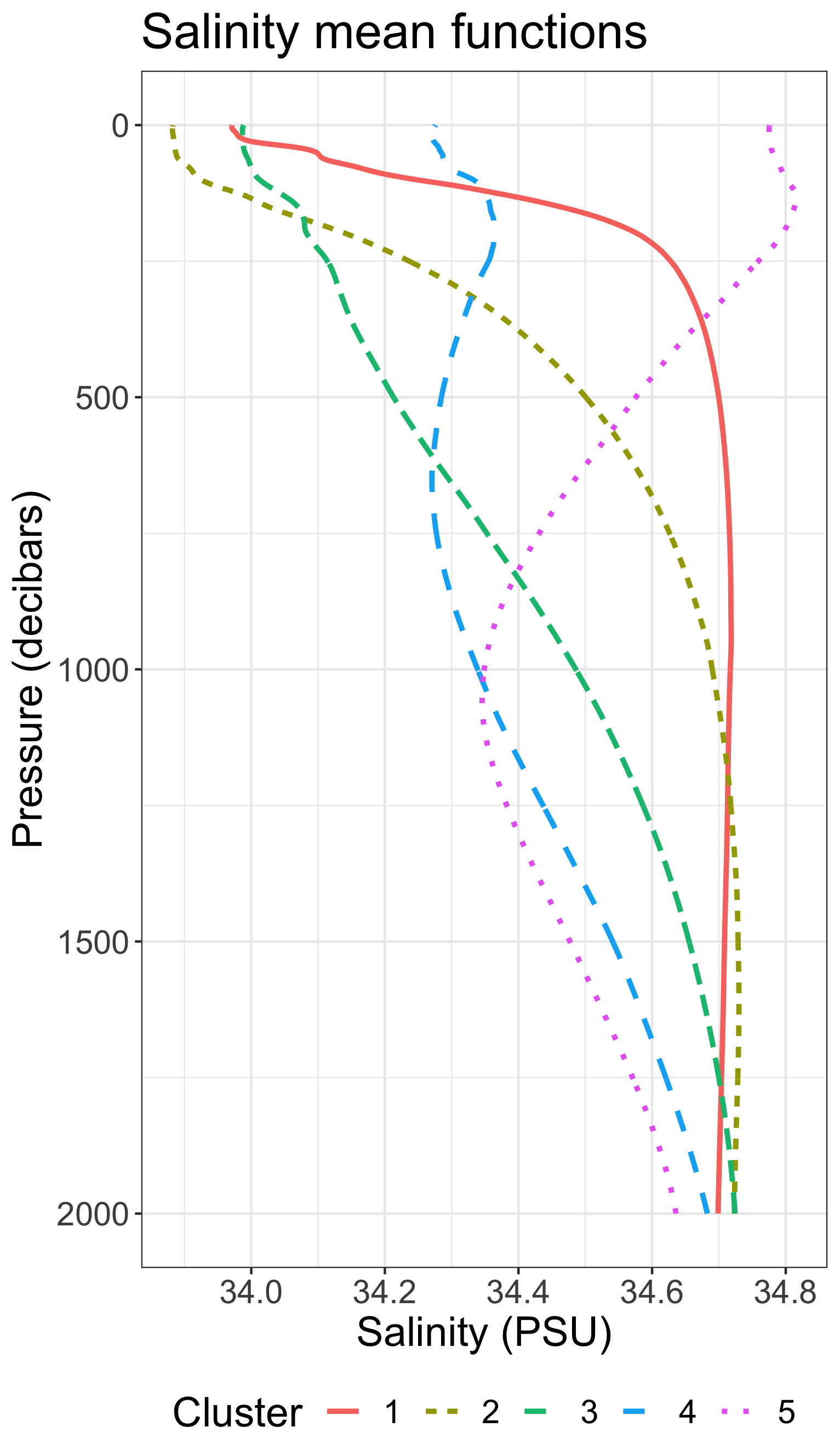
Figure S11: Temperature (left) and salinity (right) means for each cluster.

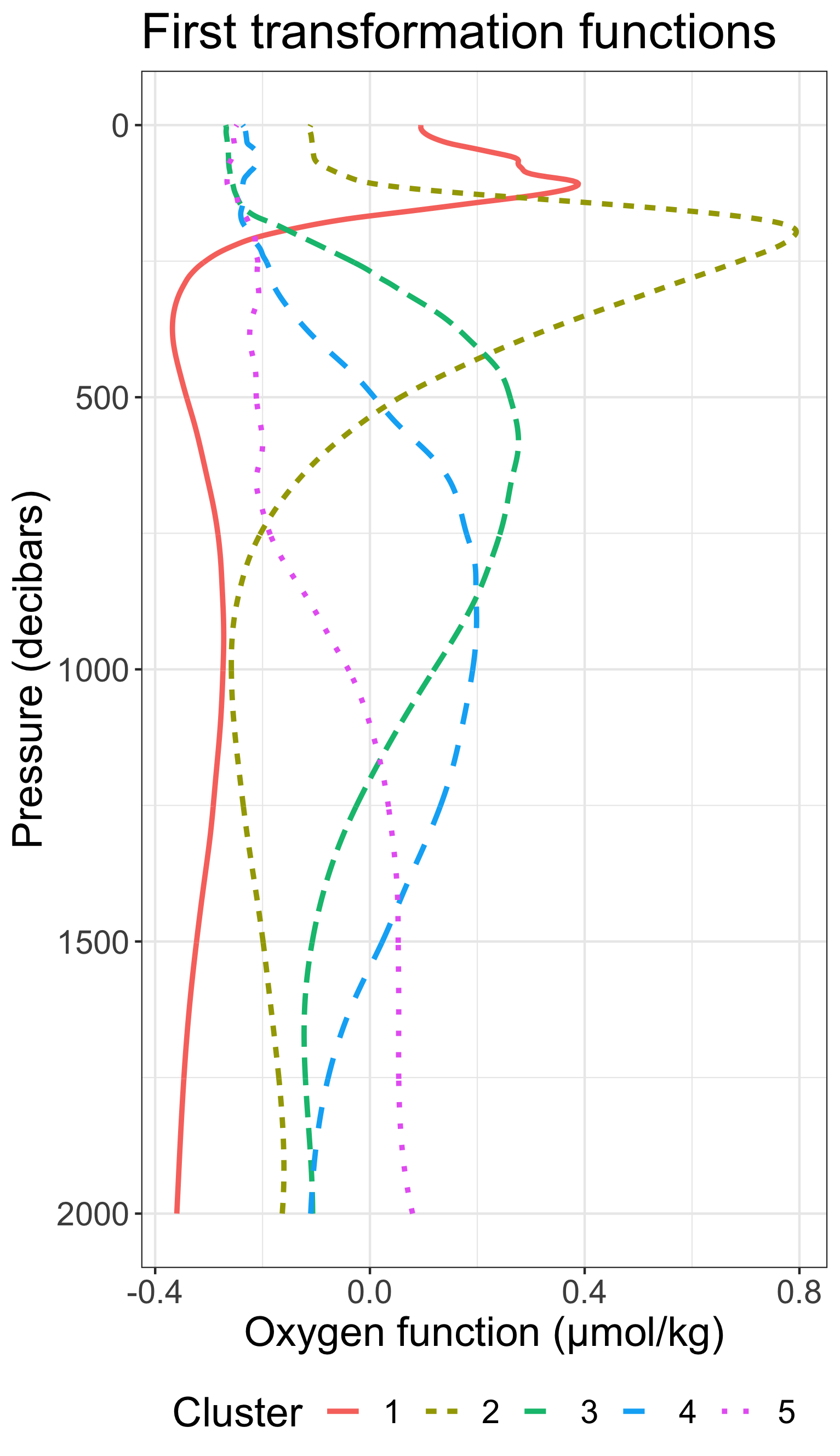
Figure S12: The first estimated functions for each group, for a) temperature PCs, b) salinity PCs, c) linear transformation functions, d) principal components of $\mathcal{E}$.

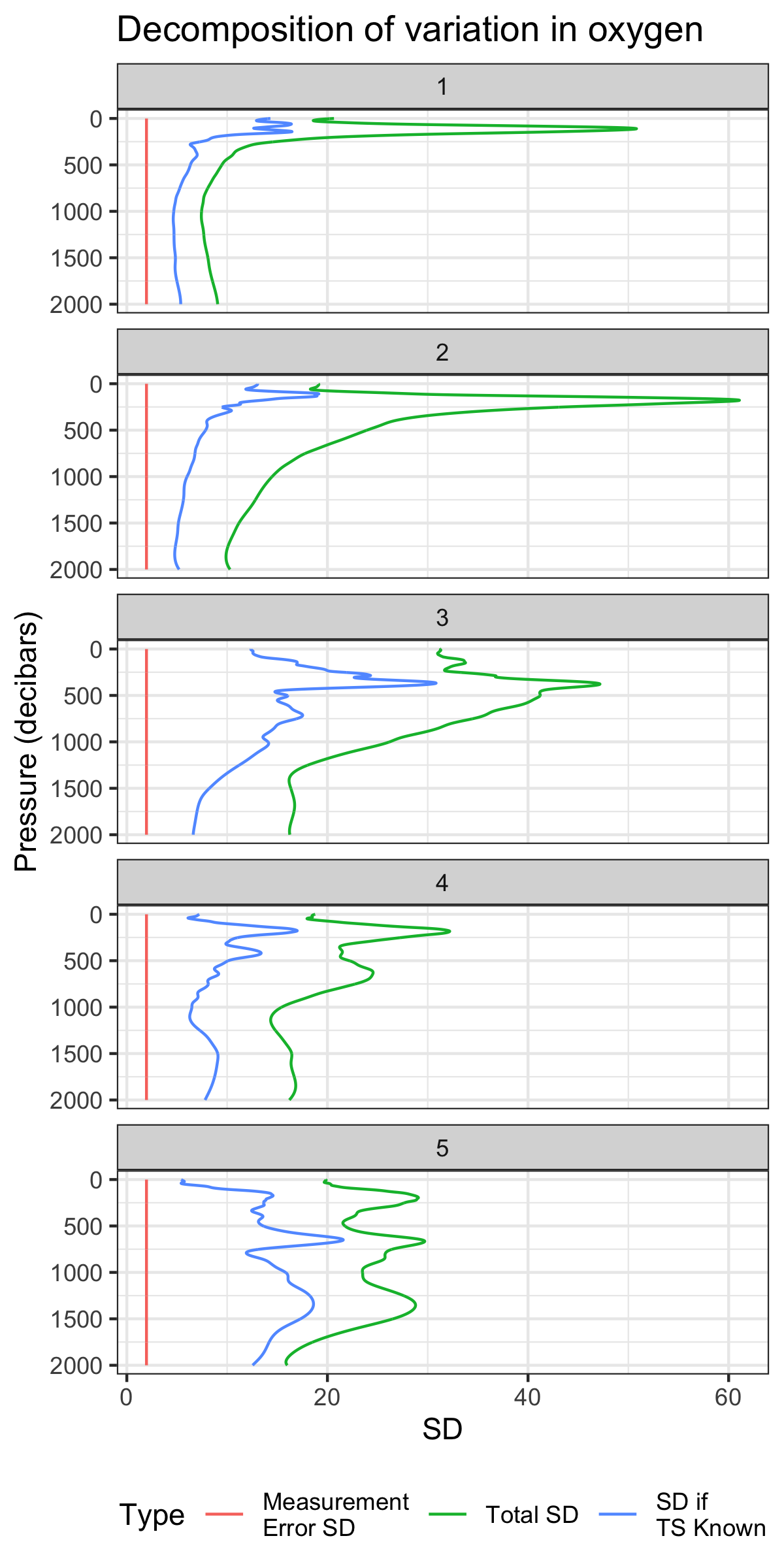
Figure S13: Breakdown of oxygen variability by cluster based on the model). Measurement error standard deviation refers to $\sigma_{Y}$, standard deviation where temperature and salinity is known is $\sqrt{\sigma_{Y}^{2}+B(p)\Theta_{\mathcal{Y},g}\mathbb{V}\textrm{ar}(\eta_{g})\Theta_{\mathcal{Y},g}^{\top}B(p)^{\top}}$, while the total standard deviation is $\sqrt{\sigma_{Y}^{2}+B(p)\Lambda_{g}\mathbb{V}\textrm{ar}(\alpha_{g})\Lambda_{g}^{\top}B(p)^{\top}+B(p)\Theta_{\mathcal{Y},g}\mathbb{V}\textrm{ar}(\eta_{g})\Theta_{\mathcal{Y},g}^{\top}B(p)^{\top}}$.

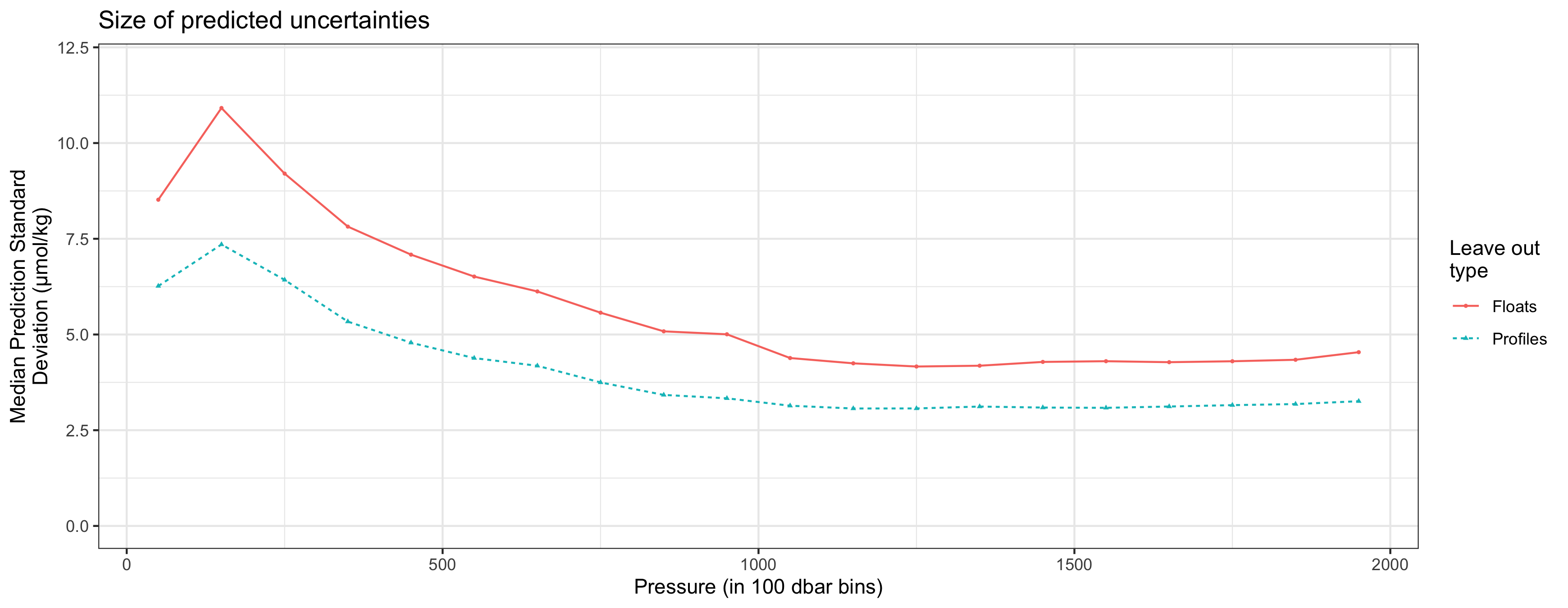
Figure S14: The median predicted standard deviations for leave-out experiments, by pressure.

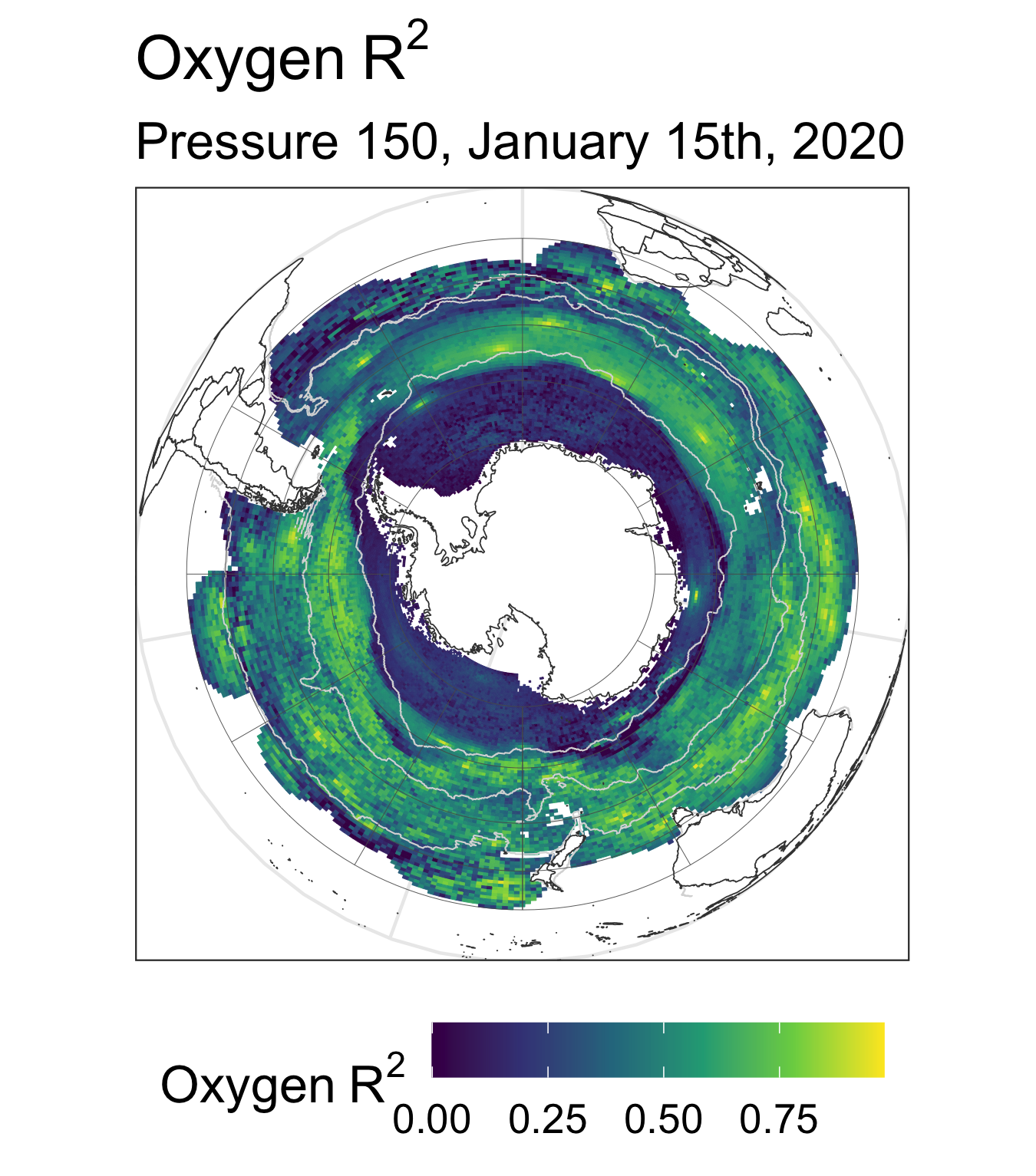
Figure S15: Proportion of oxygen variance explained by the covariates and spatial correlation in prediction, January 15, 2020.

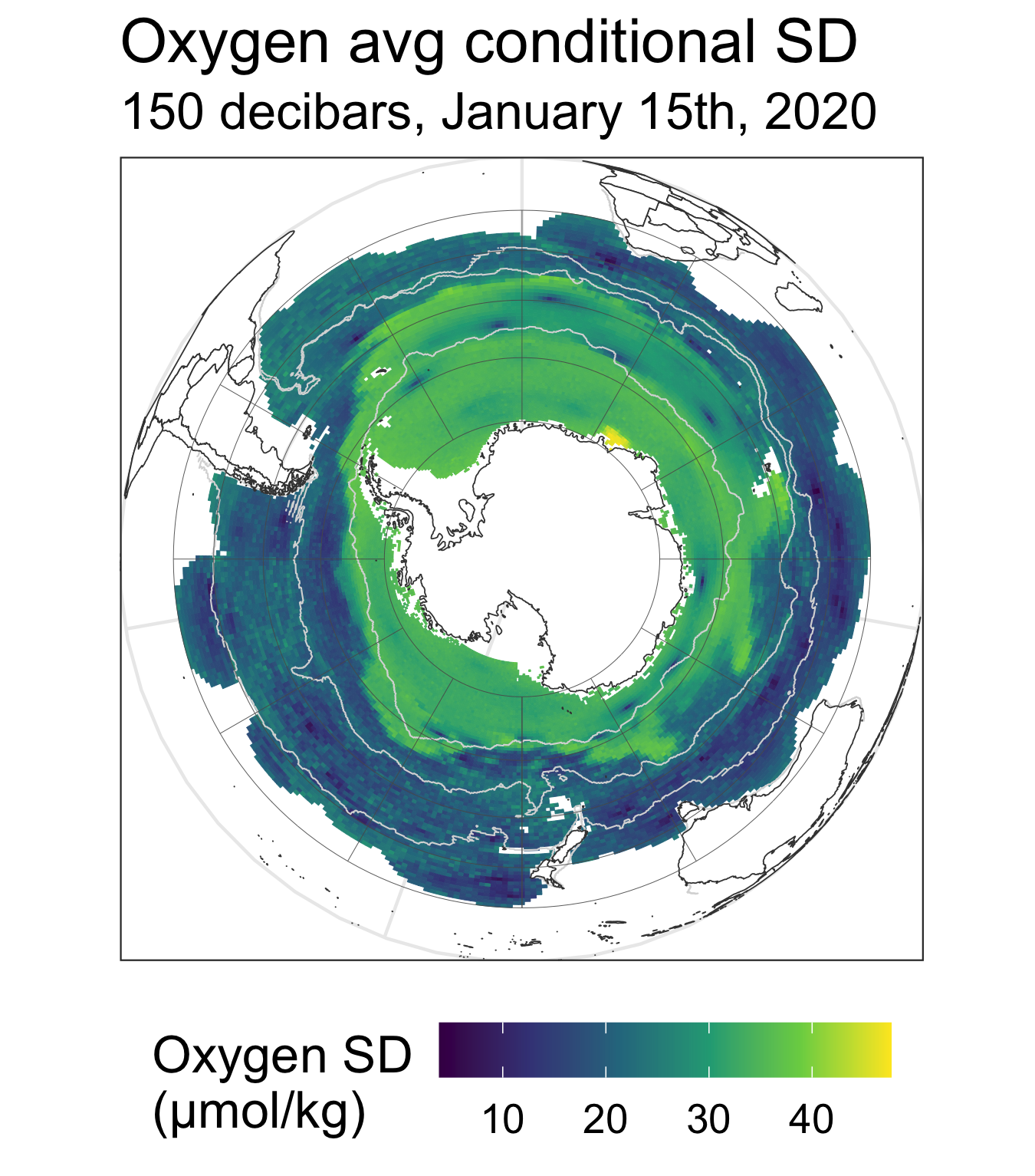
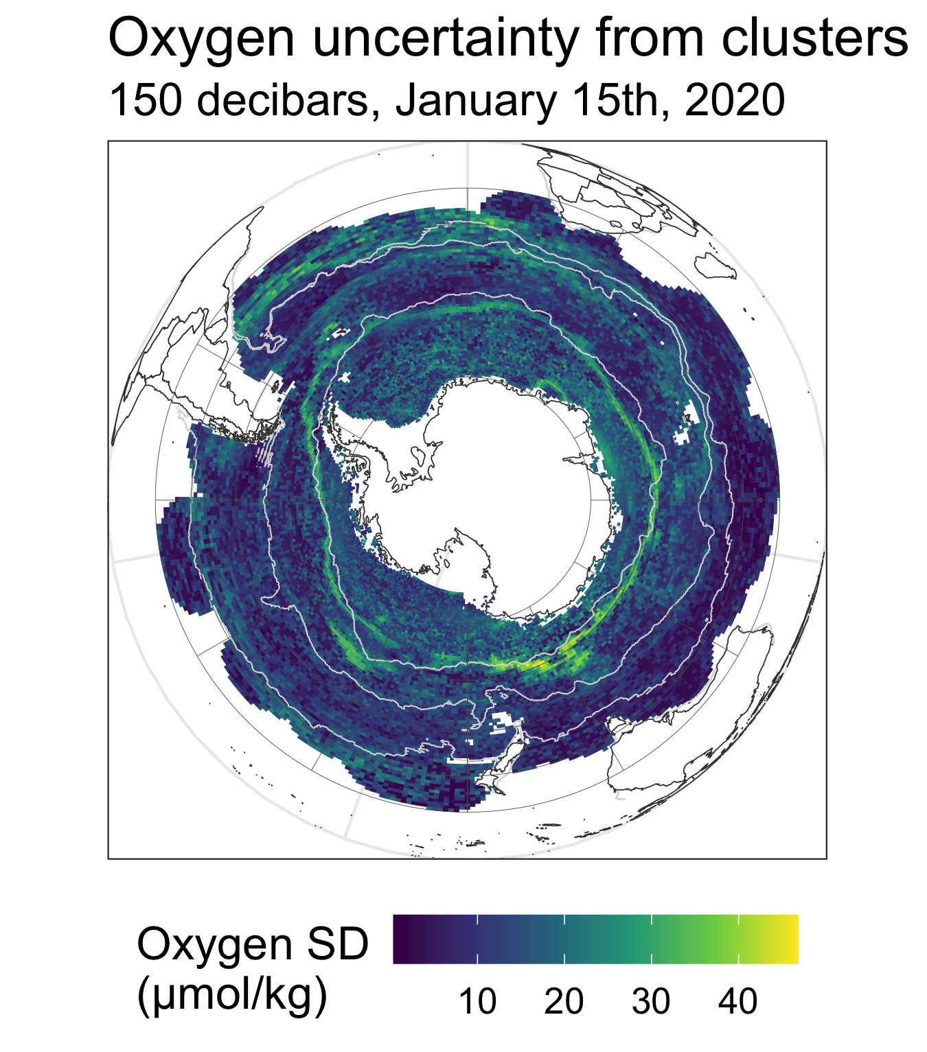
Figure S16: (Left) Model-based uncertainty of oxygen based on the scores in term (10) for January 15th, 2020 at 150 decibars. (Right) Model-uncertainty based on the clustering in term (11). The combination of this uncertainty represents the overall uncertainty in the oxygen estimates.

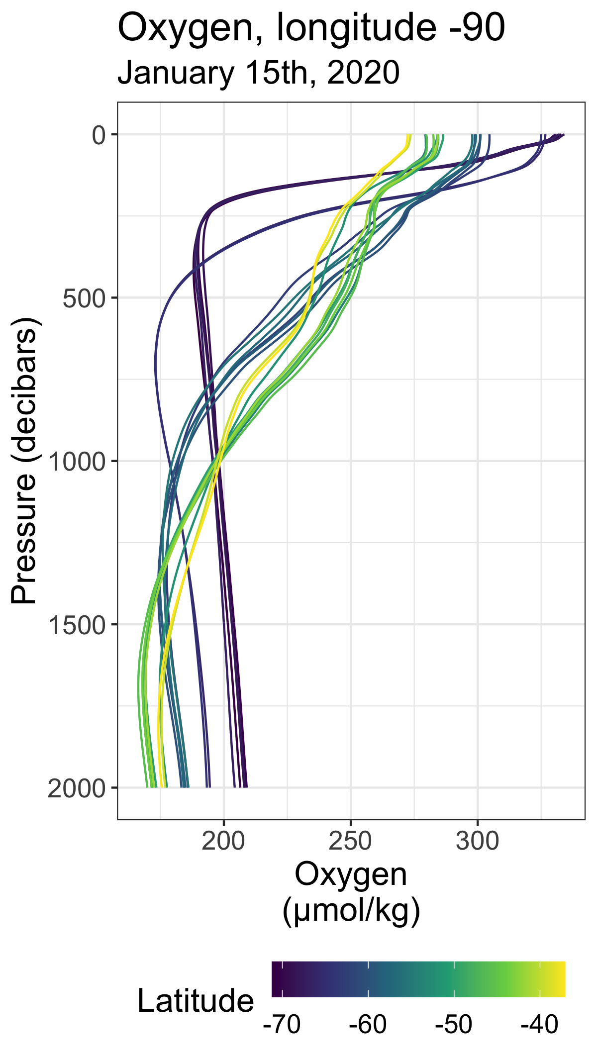
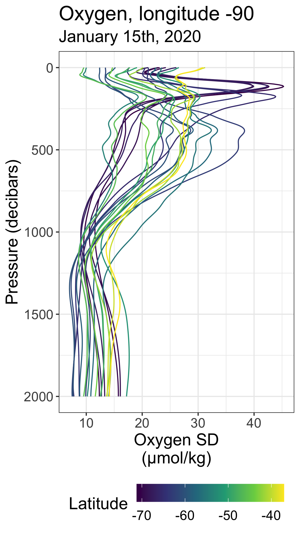
Figure S17: Estimated oxygen (left) and oxygen standard deviation (right) for longitude -90^∘ for varying latitude and pressure. As one moves from south (dark) to north (light), the predicted oxygen and their uncertainties take different shapes.

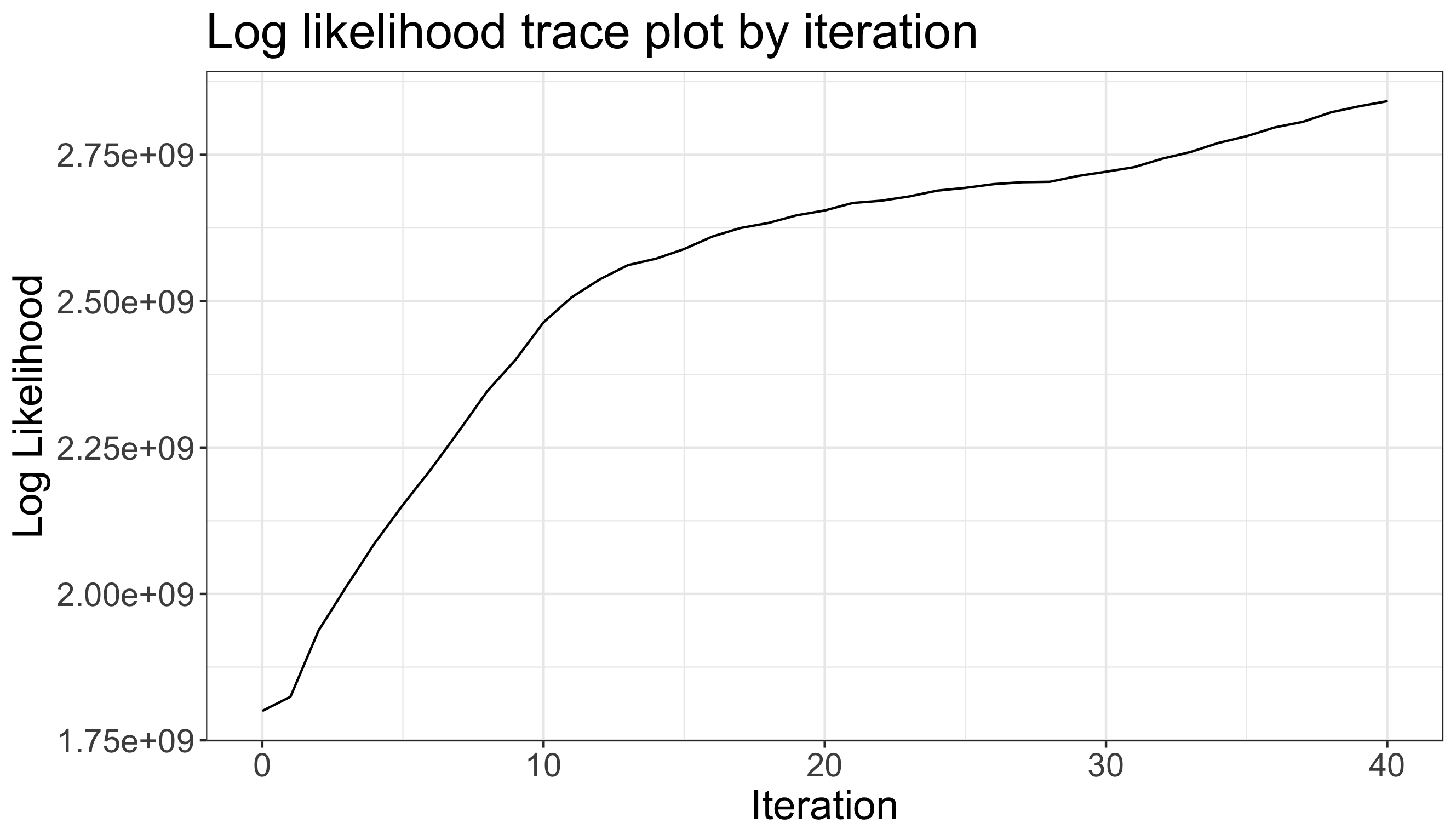
Figure S18: Log-likelihood $\widehat{f(\boldsymbol{X},\boldsymbol{Y})}$ for each MC iteration when considering $G=5$, $Q_{1}=Q_{2}=12$.

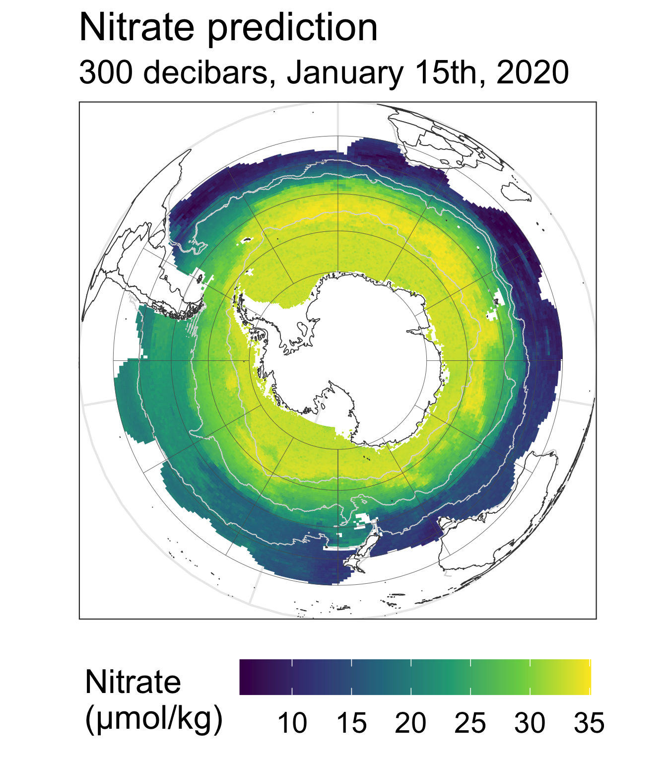
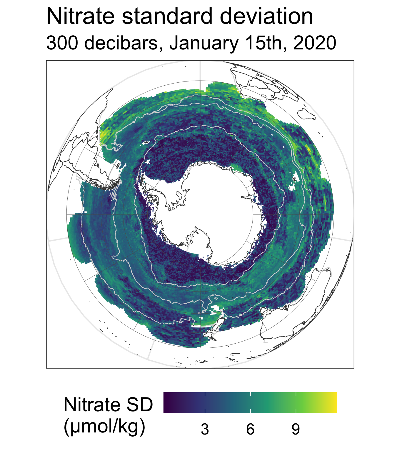
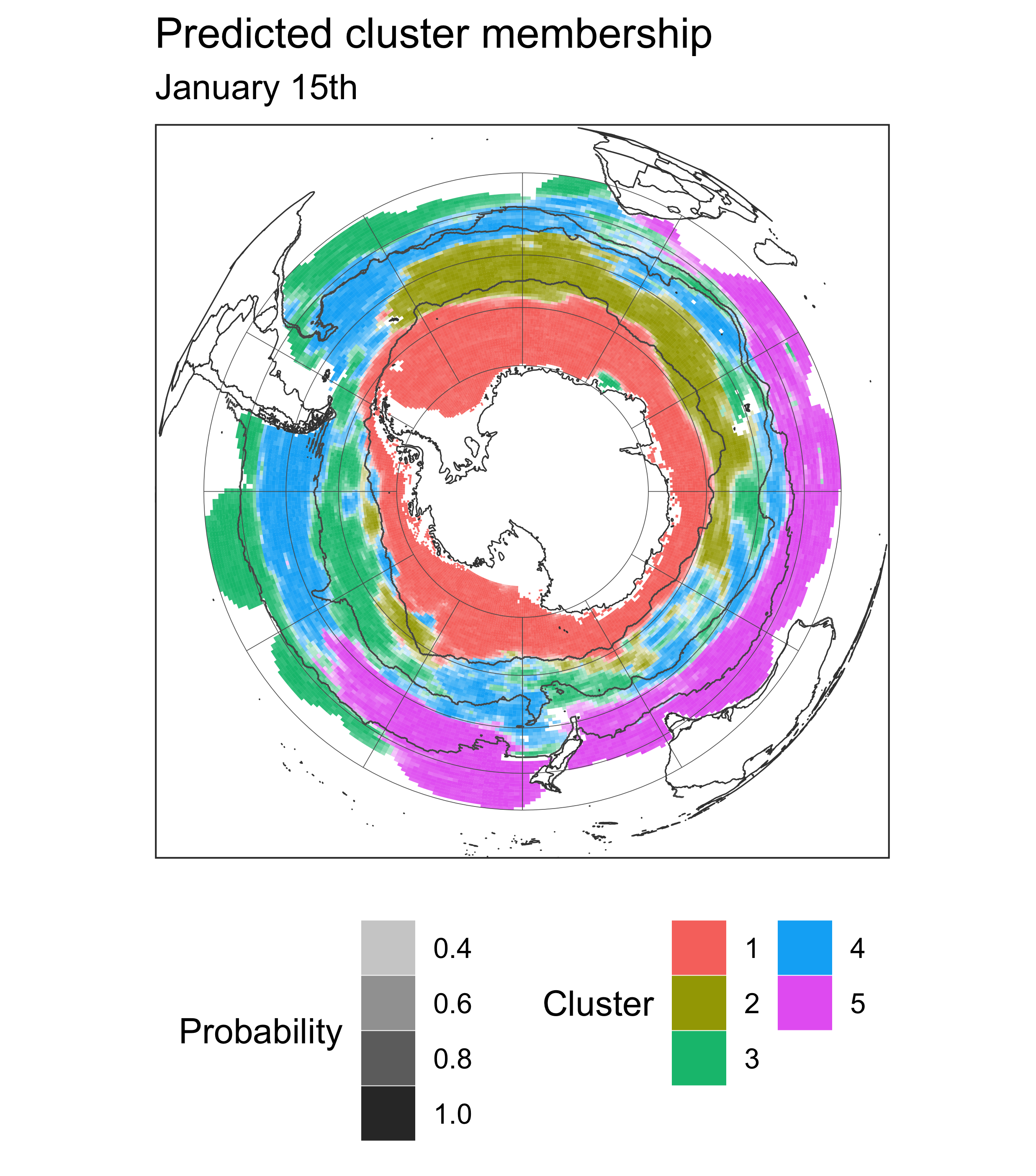
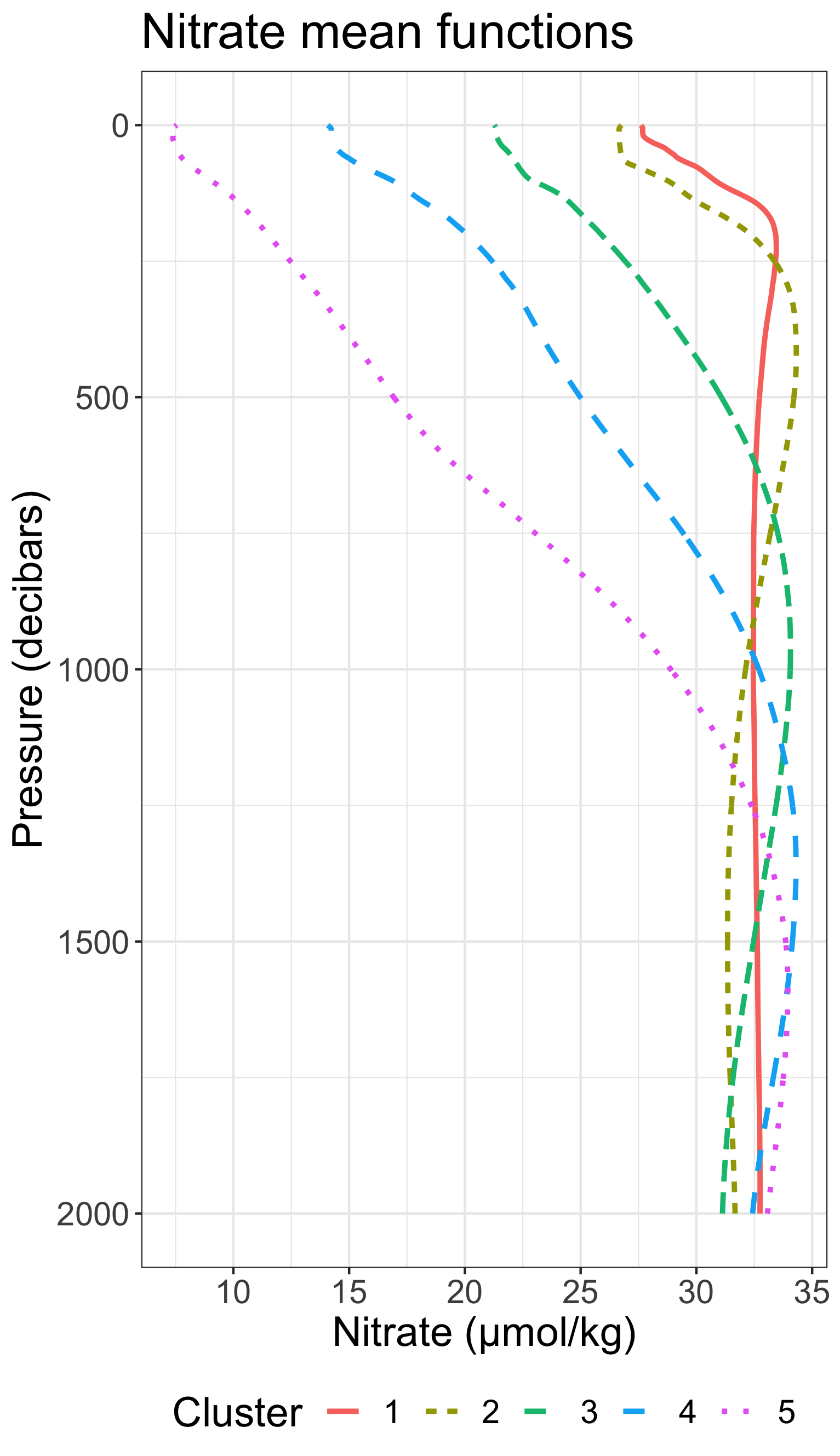
Figure S19: (Far Left) Nitrate prediction for January 15th, 2020 at 300 decibars, based on 5 clusters. (Left) Nitrate prediction standard deviation for the same quantities. (Right) Cluster membership map for January 15, 2020. (Far Right) Mean nitrate functions for each cluster.

References

• Argo, (2020) Argo (2020). Argo float data and metadata from Global Data Assembly Centre (Argo GDAC).
• Besag, (1975) Besag, J. (1975). Statistical analysis of non-lattice data. Journal of the Royal Statistical Society. Series D (The Statistician), 24(3):179–195.
• Bittig et al., (2019) Bittig, H. C., Maurer, T. L., Plant, J. N., Schmechtig, C., Wong, A. P. S., Claustre, H., …, and Xing, X. (2019). A BGC-Argo guide: planning, deployment, data handling and usage. Frontiers in Marine Science, 6.
• Bittig et al., (2018) Bittig, H. C., Steinhoff, T., Claustre, H., Fiedler, B., Williams, N. L., Sauzède, R., Körtzinger, A., and Gattuso, J.-P. (2018). An alternative to static climatologies: Robust estimation of open ocean CO2 variables and nutrient concentrations from T, S, and O2 data using Bayesian Neural Networks. Frontiers in Marine Science, 5.
• Bolin et al., (2019) Bolin, D., Wallin, J., and Lindgren, F. (2019). Latent Gaussian random field mixture models. Computational Statistics & Data Analysis, 130:80–93.
• Bushinsky et al., (2017) Bushinsky, S. M., Gray, A. R., Johnson, K. S., and Sarmiento, J. L. (2017). Oxygen in the Southern Ocean from Argo floats: determination of processes driving air-sea fluxes. Journal of Geophysical Research: Oceans, 122(11):8661–8682.
• Byrd et al., (1995) Byrd, R. H., Lu, P., Nocedal, J., and Zhu, C. (1995). A limited memory algorithm for bound constrained optimization. SIAM Journal on Scientific Computing, 16(5):1190–1208.
• Chapman et al., (2020) Chapman, C. C., Lea, M.-A., Meyer, A., Sallée, J.-B., and Hindell, M. (2020). Defining Southern Ocean fronts and their influence on biological and physical processes in a changing climate. Nature Climate Change, 10(3):209–219.
• Claustre et al., (2020) Claustre, H., Johnson, K. S., and Takeshita, Y. (2020). Observing the global ocean with Biogeochemical-Argo. Annual Review of Marine Science, 12(1):23–48.
• Dempster et al., (1977) Dempster, A. P., Laird, N. M., and Rubin, D. B. (1977). Maximum likelihood from incomplete data via the EM algorithm. Journal of the Royal Statistical Society: Series B (Methodological), 39(1):1–22.
• Feng et al., (2012) Feng, D., Tierney, L., and Magnotta, V. (2012). MRI tissue classification using high-resolution Bayesian hidden Markov normal mixture models. Journal of the American Statistical Association, 107(497):102–119.
• Fetterer et al., (2017) Fetterer, F., Knowles, K., Meier, W., Savoie, M., and Windnagel, A. (2017). Sea Ice Index, Version 3.
• Frévent et al., (2021) Frévent, C., Ahmed, M.-S., Marbac, M., and Genin, M. (2021). Detecting spatial clusters in functional data: new scan statistic approaches. Spatial Statistics, 46:100550.
• Giglio et al., (2018) Giglio, D., Lyubchich, V., and Mazloff, M. R. (2018). Estimating oxygen in the Southern Ocean using Argo temperature and salinity. Journal of Geophysical Research: Oceans, 123(6):4280–4297.
• Guinness, (2021) Guinness, J. (2021). Gaussian process learning via Fisher scoring of Vecchia’s approximation. Statistics and Computing, 31(3):25.
• Guinness et al., (2021) Guinness, J., Katzfuss, M., and Fahmy, Y. (2021). Fast Gaussian Process Computation Using Vecchia’s Approximation. R package version 0.3.2.
• Happ and Greven, (2018) Happ, C. and Greven, S. (2018). Multivariate functional principal component analysis for data observed on different (dimensional) domains. Journal of the American Statistical Association, 113(522):649–659.
• Houghton and Wilson, (2020) Houghton, I. A. and Wilson, J. D. (2020). El Niño detection via unsupervised clustering of Argo temperature profiles. Journal of Geophysical Research: Oceans, 125(9).
• Hsing and Eubank, (2015) Hsing, T. and Eubank, R. (2015). Theoretical Foundations of Functional Data Analysis, with an Introduction to Linear Operators. Wiley Series in Probability and Statistics. John Wiley and Sons, Inc.
• Huang et al., (2014) Huang, H., Li, Y., and Guan, Y. (2014). Joint modeling and clustering paired generalized longitudinal trajectories with application to cocaine abuse treatment data. Journal of the American Statistical Association, 109(508):1412–1424.
• Ibrahim et al., (2008) Ibrahim, J. G., Zhu, H., and Tang, N. (2008). Model selection criteria for missing-data problems using the EM algorithm. Journal of the American Statistical Association, 103(484):1648–1658.
• Jiang and Serban, (2012) Jiang, H. and Serban, N. (2012). Clustering Random Curves Under Spatial Interdependence With Application to Service Accessibility. Technometrics, 54(2):108–119.
• Johnson et al., (2020) Johnson, K. S., Riser, S. C., Boss, E. S., Talley, L. D., Sarmiento, J. L., Swift, D. D., Plant, J. N., Maurer, T. L., Key, R. M., Williams, N. L., Wanninkhof, R. H., Dickson, A. G., Feely, R. A., and Russell, J. L. (2020). SOCCOM float data - Snapshot 2020-08-30.
• Jones et al., (2019) Jones, D. C., Holt, H. J., Meijers, A. J. S., and Shuckburgh, E. (2019). Unsupervised clustering of Southern Ocean Argo float temperature profiles. Journal of Geophysical Research: Oceans, 124(1):390–402.
• Keeling et al., (2010) Keeling, R. F., Körtzinger, A., and Gruber, N. (2010). Ocean deoxygenation in a warming world. Annual Review of Marine Science, 2(1):199–229.
• Kuusela and Stein, (2018) Kuusela, M. and Stein, M. L. (2018). Locally stationary spatio-temporal interpolation of Argo profiling float data. Proceedings of the Royal Society A: Mathematical, Physical and Engineering Sciences, 474(2220).
• Liang et al., (2020) Liang, D., Zhang, H., Chang, X., and Huang, H. (2020). Modeling and regionalization of China’s PM${}_{\textrm{2.5}}$ using spatial-functional mixture models. Journal of the American Statistical Association, pages 1–17.
• Liang et al., (2018) Liang, Y.-C., Mazloff, M. R., Rosso, I., Fang, S.-W., and Yu, J.-Y. (2018). A multivariate empirical orthogonal function method to construct nitrate maps in the Southern Ocean. Journal of Atmospheric and Oceanic Technology, 35(7):1505–1519.
• Margaritella et al., (2021) Margaritella, N., Inácio, V., and King, R. (2021). Parameter clustering in Bayesian functional principal component analysis of neuroscientific data. Statistics in Medicine, 40(1):167–184.
• Maurer et al., (2021) Maurer, T. L., Plant, J. N., and Johnson, K. S. (2021). Delayed-mode quality control of oxygen, nitrate, and pH data on SOCCOM biogeochemical profiling floats. Frontiers in Marine Science, 8:1118.
• Maze et al., (2017) Maze, G., Mercier, H., Fablet, R., Tandeo, P., Lopez Radcenco, M., Lenca, P., Feucher, C., and Le Goff, C. (2017). Coherent heat patterns revealed by unsupervised classification of Argo temperature profiles in the North Atlantic Ocean. Progress in Oceanography, 151:275–292.
• Mignot et al., (2019) Mignot, A., D’Ortenzio, F., Taillandier, V., Cossarini, G., and Salon, S. (2019). Quantifying observational errors in Biogeochemical-Argo oxygen, nitrate, and chlorophyll a concentrations. Geophysical Research Letters, 46(8):4330–4337.
• Orsi et al., (1995) Orsi, A. H., Whitworth, T., and Nowlin, W. D. (1995). On the meridional extent and fronts of the Antarctic Circumpolar Current. Deep Sea Research Part I: Oceanographic Research Papers, 42(5):641–673.
• Robert and Casella, (2004) Robert, C. P. and Casella, G. (2004). Monte Carlo Statistical Methods. Springer Texts in Statistics. Springer, New York, NY.
• Roemmich and Gilson, (2009) Roemmich, D. and Gilson, J. (2009). The 2004–2008 mean and annual cycle of temperature, salinity, and steric height in the global ocean from the Argo Program. Progress in Oceanography, 82(2):81–100.
• Rosso et al., (2020) Rosso, I., Mazloff, M. R., Talley, L. D., Purkey, S. G., Freeman, N. M., and Maze, G. (2020). Water mass and biogeochemical variability in the Kerguelen Sector of the Southern Ocean. Journal of Geophysical Research: Oceans, 125(3).
• Stein, (2013) Stein, M. L. (2013). Interpolation of Spatial Data: Some Theory for Kriging. Springer.
• Stoehr et al., (2016) Stoehr, J., Marin, J.-M., and Pudlo, P. (2016). Hidden Gibbs random fields model selection using block likelihood information criterion. Stat, 5(1):158–172.
• Stramma and Schmidtko, (2021) Stramma, L. and Schmidtko, S. (2021). Spatial and temporal variability of oceanic oxygen changes and underlying trends. Atmosphere-Ocean, 59(2):122–132.
• Thomas et al., (2021) Thomas, S. D. A., Jones, D. C., Faul, A., Mackie, E., and Pauthenet, E. (2021). Defining Southern Ocean fronts using unsupervised classification. Ocean Science Discussions, 17:1545–1562.
• Verdy and Mazloff, (2017) Verdy, A. and Mazloff, M. R. (2017). A data assimilating model for estimating Southern Ocean biogeochemistry. Journal of Geophysical Research: Oceans, 122(9):6968–6988.
• Wei and Tanner, (1990) Wei, G. C. G. and Tanner, M. A. (1990). A Monte Carlo implementation of the EM algorithm and the Poor Man’s data augmentation algorithms. Journal of the American Statistical Association, 85(411):699–704.
• Wei and Zhou, (2010) Wei, J. and Zhou, L. (2010). Model selection using modified AIC and BIC in joint modeling of paired functional data. Statistics & Probability Letters, 80(23):1918–1924.
• Williams et al., (2016) Williams, N. L., Juranek, L. W., Johnson, K. S., Feely, R. A., Riser, S. C., Talley, L. D., Russell, J. L., Sarmiento, J. L., and Wanninkhof, R. (2016). Empirical algorithms to estimate water column pH in the Southern Ocean. Geophysical Research Letters, 43(7):3415–3422.
• Yao et al., (2005) Yao, F., Müller, H.-G., and Wang, J.-L. (2005). Functional linear regression analysis for longitudinal data. The Annals of Statistics, 33(6):2873–2903.
• Yarger et al., (2022) Yarger, D., Stoev, S., and Hsing, T. (2022). A functional-data approach to the Argo data. The Annals of Applied Statistics, 16(1):216–246.
• Zhang, (2004) Zhang, H. (2004). Inconsistent estimation and asymptotically equal interpolations in model-based geostatistics. Journal of the American Statistical Association, 99(465):250–261.
• Zhang and Li, (2021) Zhang, H. and Li, Y. (2021). Unified principal component analysis for sparse and dense functional data under spatial dependency. Journal of Business & Economic Statistics, pages 1–15.
• Zheng and Serban, (2018) Zheng, Y. and Serban, N. (2018). Clustering the prevalence of pediatric chronic conditions in the United States using distributed computing. The Annals of Applied Statistics, 12(2).
• Zhou et al., (2008) Zhou, L., Huang, J., and Carroll, R. (2008). Joint modeling of paired sparse functional data using principal components. Biometrika, 95:601–619.
• Zhou et al., (2010) Zhou, L., Huang, J. Z., Martinez, J. G., Maity, A., Baladandayuthapani, V., and Carroll, R. J. (2010). Reduced rank mixed effects models for spatially correlated hierarchical functional data. Journal of the American Statistical Association, 105(489):390–400.