Splitting expands the application range of vision transformer
Variable Vision Transformer (vViT)

Abstract

Vision Transformer (ViT) has achieved outstanding results in computer vision. Although there are many Transformer-based architectures derived from the original ViT, the dimension of patches are often the same with each other. This disadvantage leads to a limited application range in the medical field because in the medical field, datasets whose dimension is different from each other; e.g. medical image, patients’ personal information, laboratory test and so on. To overcome this limitation, we develop a new derived type of ViT termed variable Vision Transformer (vViT). The aim of this study is to introduce vViT and to apply vViT to radiomics using T1 weighted magnetic resonance image (MRI) of glioma. In the prediction of 365 days of survival among glioma patients using radiomics,vViT achieved 0.83, 0.82, 0.81, and 0.76 in sensitivity, specificity, accuracy, and AUC-ROC, respectively. vViT has the potential to handle different types of medical information at once.

1 Introduction

Self attention-based architectures, especially Transformer have achieved outstanding results (Vaswani et al., 2017). In this study, Vaswani et al. showed that Transformer reduced the calculation cost while keeping the performance of the recurrent neural network (RNN) in the translation task. Transformer has the potential to supersede other RNN-based models such as long short-term memory and gated RNN (Hochreiter & Schmidhuber, 1997; Chung et al., 2014). In contrast to the success of Transformer in natural language processing (NLP), convolutional architectures had remained the dominant architecture in computer vision and image recognition (LeCun et al., 1989; Krizhevsky et al., 2012; He et al., 2015). This situation is partly caused by the difference between NLP and computer vision. In NLP, a token can be easily defined from a sentence. On the other hand, in the application transformer to computer vision, it is a problem with how to define an image that corresponds to the token in NLP. Dosovitskiy et al. gave a solution to this problem by splitting the image into 16×16 images (Dosovitskiy et al., 2020). Dosovitskiy et al. achieved 88.55% of accuracy using the model termed vision transformer (ViT). Although the performance of ViT was lower than that of some other convolutional architecture-based models, ViT reduces calculation costs and leads to time savings (Dosovitskiy et al., 2020). However, in analyzing a medical image, ViT has a limitation. In medical image analysis, some other features such as patients’ medical information (age, sex, medication history, physical assessment data, laboratory test data, and so on ) and radiomics features as well as the medical image itself. To analyze the information by ViT, inputs and heads dimensions should be controlled because ViT analyzes the splitted images of which dimensions are equal to each other. To overcome this limitation, we constructed a model termed variable vision transformer (vViT) which can handle variable input dimensions. As an example of variable input dimensions, we selected radiomics features regarding each group of features. The radiomics explains quantitative image features from standard-of-care medical imaging(Lambin et al., 2017). The aims of this paper are to introduce vViT and to apply vViT to radiomics using T1 weighted magnetic resonance image (MRI) of glioma.

2 Methods

In the model implementation of vViT, we follow the original ViT (Dosovitskiy et al, 2020) and Transformer (Vaswani et al., 2017) as closely as possible. In the model architecture explanation, index $p$ means patch.

2.1 vViT Model Architecture

Figure 1 shows an overview of the vViT model architecture. The standard Transformer receives as input a 1D sequence of token embeddings. vViT receives 1D sequence $\mathbb{x}\in\mathbb{R}$ and split-sequence $\{a_{n}\}(n\in\mathbb{N},a_{n}\in\mathbb{N},1\leq n\leq N)$ as an input. The input sequence $\mathbb{x}$ is divided into $N$ sequences $\{\mathbb{x}_{p}^{1},\mathbb{x}_{p}^{2},\cdots\mathbb{x}_{p}^{N}\}$ according to split-sequence $\{a_{n}\}$: the length of $\mathbb{x}_{p}^{n}$ is equal to $a_{n}(1\leq n\leq N)$. After splitting the input sequence $\mathbb{x}$ is divided into $N$ sequences $\{\mathbb{x}_{p}^{1},\mathbb{x}_{p}^{2},\cdots\mathbb{x}_{p}^{N}\}$, we perform linear transformation by $\mathbb{D}_{n}\in R^{a_{n}\times m}$ to give the same dimension $m$ to all patch.

Similar to [class] token in Bidirectional Encoder Representations from Transformers (BERT) and ViT, we prepend a learnable embedding to the sequence of embedded patches $(\mathbb{z}_{0}^{0}=\mathbb{x}_{\textrm{class}})$, whose output values of the Transformer encoder $(\mathbb{z}_{L}^{0})$ represents the sequence $\mathbb{y}$. The classification head is implemented by an MLP with one hidden layer at pre-training time and by a single linear layer at the fine-tuning time based on the previous Transformer study. We prepend the embedded patches $(\mathbb{z}_{0}^{0}=\mathbb{x}_{\textrm{class}})$ whose length is $m$.

The Transformer encoder (Vaswani et al., 2017) is composed of alternating layers of multiheaded self-attention (MSA) and multilayer perceptron (MLP) blocks. Layernorm (LN) is applied before every block, and residual connections after every block (Wang et al., 2019; Baevski and Auli, 2019). We implemented MLP using two layers with a Gaussian Error Linear Unit (GELU) non-linearity.

$$\mathbb{z}_{-1} =[\mathbb{x}_{p}^{1}\mathbb{D}_{1};\ \mathbb{x}_{p}^{2}\mathbb{D}_{2};\ \cdots;\ \mathbb{x}_{p}^{N}\mathbb{D}_{N}]\hskip 28.45274pt\mathbb{D}_{n}\in\mathbb{R}^{a_{n}\times m}$$ (1)

$$\mathbb{z}_{0} =[\mathbb{x}_{\textrm{class}};\ (\mathbb{x}_{p}^{1}\mathbb{D}_{1})\mathbb{E}_{1};\ (\mathbb{x}_{p}^{2}\mathbb{D}_{2})\mathbb{E}_{2};\ \cdots;\ (\mathbb{x}_{p}^{N}\mathbb{D}_{N})\mathbb{E}_{N}]+\mathbb{E}_{\textrm{pos}}$$ (2)

$$\hskip 28.45274pt\mathbb{E}_{n}\in\mathbb{R}^{m\times d},\ \mathbb{E}_{\textrm{pos}}\in\mathbb{R}^{(N+1)\times d}$$

$$\mathbb{z}^{\prime}_{\ell} =\textrm{MSA}(\textrm{LN}(z_{\ell-1}))+z_{\ell-1}\hskip 28.45274pt\ell=1,2,\cdots,L,$$ (3)

$$\mathbb{z}_{\ell} =\textrm{MLP}(\textrm{LN}(z_{\ell}^{\prime}))+z_{\ell}^{\prime}\hskip 49.79231pt\ell=1,2,\cdots,L,$$ (4)

$$\mathbb{y} =\textrm{LN}(z_{L}^{0}).$$ (5)

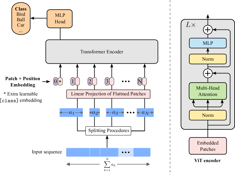
Figure 1: vViT model architecture. We split an image into flexible-size patches according to split sequence, linearly embed each of them, add position embeddings, and feed the resulting sequence of vectors to a standard Transformer encoder. To perform classification, we add an extra learnable embedding [class] to the sequence. The illustration of the Transformer encoder was inspired by (Vaswani et al., 2017; Dosovitskiy et al., 2020)

2.2 Experiments

The images used for analysis were obtained from The University of California San Francisco Preoperative Diffuse Glioma MRI (UCSF-PDGM) published in the Image Cancer Archive (TCIA) (Calabrese et al., 2022; Clark et al., 2013). The UCSF-PDGM dataset includes 501 subjects with histopathologically-proven diffuse gliomas who were imaged with a standardized 3 Tesla preoperative brain tumor MRI protocol featuring predominantly 3D imaging, as well as advanced diffusion and perfusion imaging techniques. Multicompartment tumor segmentation of study data was undertaken as part of the 2021 BraTS challenge. Image data first underwent automated segmentation using an ensemble model consisting of prior BraTS challenge-winning segmentation algorithms. Images were then manually corrected by trained radiologists and approved by 2 expert reviewers. Segmentation included three major tumor compartments: enhancing tumor, non-enhancing/necrotic tumor, and surrounding FLAIR abnormality (sometimes referred to as edema). The UCSF-PDGM adds to an existing body of publicly available diffuse glioma MRI datasets that are commonly used in AI research applications. As MRI-based AI research applications continue to grow, new data are needed to foster the development of new techniques and increase the generalizability of existing algorithms. The UCSF-PDGM not only significantly increases the total number of publicly available diffuse glioma MRI cases, but also provides a unique contribution in terms of MRI technique. The inclusion of 3D sequences and advanced MRI techniques like ASL and HARDI provides a new opportunity for researchers to explore the potential utility of cutting-edge clinical diagnostics for AI applications. The details of UCSF-PDGM are explained somewhere else (Calabrese et al., 2022; Clark et al., 2013).

The T1 weighted MRI images and tumor mask images were used to calculate radiomic features. We excluded the images whose mask images contain 16 pixels or lower 16 pixels. After this exclusion, 10,538 images remained. Using PyRadiomics (van Griethuysen et al., 2017), 104 radiomic features were extraxted; 19 First Order features (Energy, Total Energy, Entropy, Minimum, 10 Percentile, 90 Percentile, Maximum, Mean, Median, Range, Interquartile Range, Mean Absolute Deviation, Robust Mean Absolute Deviation, Root Mean Squared, Standard Deviation, Skewness, Kurtosis, Variance, and Uniformity), 10 Shape2D features (Mesh Surface, Pixel Surface, Perimeter, Perimeter Surface Ratio, Sphericity, Spherical Disproportion, Maximum Diameter, Major Axis Length, Minor Axis Length, and Elongation), 24 Gray-Level Co-occurrence Matrix (GLCM) fetures (Autocorrelation, Joint Average, Cluster Prominence, Cluster Shade, Cluster Tendency, Contrast, Correlation, Difference Average, Difference Entropy, Difference Variance, Joint Energy, Joint Entropy, Informational Measure of Correlation 1, Informational Measure of Correlation 2, Inverse Difference Moment, Maximal Correlation Coefficient, Inverse Difference Moment Normalized, Inverse Difference, Inverse Difference Normalized, Inverse Variance, Maximum Probability, Sum Average, Sum Entropy, and Sum Squares), 16 Gray Level Size Zone Matrix (GLSZM) features (Small Area Emphasis, Large Area Emphasis, Gray Level Non Uniformity, Gray Level Non Uniformity Normalized, Size Zone Non Uniformity, Size Zone Non Uniformity Normalized, Zone Percentage, Gray Level Variance, Zone Variance, Zone Entropy, Low Gray Level Zone Emphasis, High Gray Level Zone Emphasis, Small Area Low Gray Level Emphasis, Small Area High Gray Level Emphasis, Large Area Low Gray Level Emphasis, and Large Area High Gray Level Emphasis), 16 Gray Level Run Length Matrix (GLRLM) features (Short Run Emphasis, Long Run Emphasis, Gray Level Non Uniformity, Gray Level Non Uniformity Normalized, Run Length Non Uniformity, Run Length Non Uniformity Normalized, Run Percentage, Gray Level Variance, Run Entropy, Run Variance, Low Gray Level Run Emphasis, High Gray Level Run Emphasis, Short Run Low Gray Level Emphasis, Short Run High Gray Level Emphasis, Long Run Low Gray Level Emphasis, and Long Run High Gray Level Emphasis), 5 Neighbouring Gray Tone Difference Matrix (NGTDM) features (Busyness, Coarseness, Complexity, Contrast, and Strength), and 14 Gray Level Dependence Matrix (GLDM) features (Small Dependence Emphasis, Large Dependence Emphasis, Gray Level Non Uniformity, Dependence Non Uniformity, Dependence Non Uniformity Normalized, Gray Level Variance, Dependence Variance, Dependence Entropy, Low Gray Level Emphasis, High Gray Level Emphasis, Small Dependence Low Gray Level Emphasis, Small Dependence High Gray Level Emphasis, Large Dependence Low Gray Level Emphasis, and Large Dependence High Gray Level Emphasis). Each group of radiomic features was separately input to vViT.

2.3 Training and Fine Tuning

We divided 10,538 slices into the training dataset (7376 slices) and test dataset (3162 slices), and the training dataset was used to train vViT. Binary cross entropy and Adaptive Moment Estimation (Adam) was used for calculating loss and optimizing, respectively. The parameters of Adam were set as learning rate (lr)$=0.0001$, $\beta=(0.9,0.999)$, $\epsilon=1.0\times 10^{-8}$, weight decay$=0$, and amsgrad=False. The scheduler was used to update the previous lr to $0.99\times$lr at the end of each epoch. The training process was repeated 600 times. After training, the test dataset was used to calculate metrics.

2.4 Metrics

The outcome was defined 1-year survival during follow-up. The information on survival was derived from UCSF-PDGM-metadata.csv published in TCIA. The radiomic feature was evaluated using mean value and standard deviation (SD). Mann–Whitney U test was performed to compare each radiomic feature between the survival and dead group. We calculated sensitivity, specificity, accuracy, and area under the curve of the receiver operating characteristics (AUC-ROC). All analyses were implemented in Python Language (Version 3.8.8).

3 Results

Table 1 and 2 in Appendix show the mean, SD, and the result of the Mann–Whitney U test for the training and test, respectively. The best sensitivity, specificity, accuracy, and AUC-ROC were 0.83, 0.82, 0.81, and 0.76, respectively. Figures 2 and 3 show the ROC and changes in sensitivity, specificity, positive predictive value, and negative predicting value, respectively.

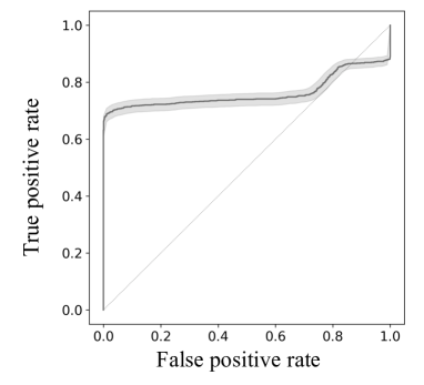
Figure 2: ROC is shown. The gray area in the figure shows 95% confidence interval. The AUC-ROC achieved by vViT was 0.76.

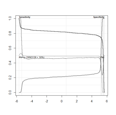
Figure 3: The changes in sensitivity, specificity, positive predicting value, and negative predicting value.

4 Discussion

In this paper, we introduced vViT and applied it to predict the 1-year survival of glioma patients using radiomics which was extracted from T1 weighted MRI. vViT achieved 0.81 and 0.76 of accuracy and AUC-ROC, respectively. vViT can handle dataset which contains different dimension subdataset by split-sequence. For example, in this paper, First Order features and Shape 2D features had 19 and 10 features, respectively. When these data are input into a deep learning model, it is controversial how to input into the model. One solution is merging and treating First Order features and Shape 2D features as one sequence. However, this approach leads to losing the information that these features are different from each other. In addition to this, in convolutional architectures, near values in the sequence tend to be convoluted. There is another problem whether these two features are similar to each other. Thus, there is a need for a new architecture that learns features remaining the difference of features. vViT has the potential to be a solution to this problem.

Some previous studies have examined the association between radiomic features and the prognosis of glioma. Remigio et al. used DeepSurv and PMF-NN models to perform convolutional architectures-based survival analysis in the task of predicting survival at 1050 days (Adrian et al., 2022; Katzman et al., 2018; Pan et al., 2021). DeepSurv and PMF-NN models achieved 0.122 and 0.67 of integrated Brier score and C-index, respectively. Shaheen et al.Shaheen et al. (2022) examined overall survival using the convolutional architectures-based model. Shaheen et al. reported the best predictive value was 0.73 of AUC-ROC. To our knowledge, in the task of direct prediction of survival among glioma patients, the vViT model achieved state-of-the-art. Other glioma studies have tried to predict mutation such as isocitrate dehydrogenase (IDH) mutation and 1p/19q codeletion using machine learning methods including convolutional architectures (Gore et al., 2021). The main purpose of these studies is a non-invasive prediction of IDH mutation and 1p/19q codeletion which are associated with the prognosis of glioma. In some of these studies, patients’ medical information was used as well as radiomic features.

Our study has some limitations. First, patients’ information such as age, sex, medication history, and MRI itself was not included in the input data. Some previous studies revealed the combination of clinical information and the medical image itself contributed to the improvement of deep learning model performance. vViT has the potential to include the information by setting split sequences. Nevertheless, vViT achieved state-of-the-art in the direct prediction of patients’ survival. Further study is needed to solve this limitation. Second, in our analysis, vViT output slice-base prediction and did not output patient base prediction. This means that the prediction may differ depending on each slice. In clinical practice, patient-base prediction is needed. Analyzing the mean probability of final output from vViT may solve this problem. In conclusion, we demonstrated that vViT improved performance in the task of predicting 365 days of survival of glioma patients using radiomics features extracted from T1 weighted MRI. vViT can flexibly handle a dataset that consists of sequences with different dimensions.

Author Contributions

Guarantors of the integrity of the entire study, T.U., K.T.; study concepts/study design or data acquisition or data analysis/interpretation, T.U., K.T.; manuscript drafting or manuscript revision for important intellectual content, T.U., K.T.; approval of final version of the submitted manuscript, T.U., K.T.; agree to ensure any questions related to the work are appropriately resolved, T.U., K.T.; literature research, T.U., K.T.; experimental studies, T.U., K.T.; statistical analysis, T.U., K.T.; and manuscript editing, T.U., K.T. T.U.and K.T. equally contributed to this work.

Acknowledgments

The authors acknowledge the National Cancer Institute and the Foundation for the National Institutes of Health, and its critical role in the creation of the free publicly available UCSF-PDGM database used in this study. Data used in this research were obtained from The Cancer Imaging Archive (TCIA) sponsored by the Cancer Imaging Program, DCTD/NCI/NIH, https://wiki.cancerimagingarchive.net/display/Public/UCSF-PDGM.

Appendix A Appendix

Table 1: Radiomic features in the train dataset and results of Mann–Whitney U test

Fetures	Survival (SD)	Dead (SD)	p-value
Energy	$6\times 10^{9}(7.1\times 10^{9})$	$5.5\times 10^{9}(6.2\times 10^{9})$	0.00024
Total Energy	$6\times 10^{9}(7.1\times 10^{9})$	$5.5\times 10^{9}(6.2\times 10^{9})$	0.00024
Entropy	4.9 (1.1)	4.7 (1.2)	$<$0.0001
Minimum	$1.2\times 10^{3}(6.3\times 10^{2})$	$1\times 10^{3}(5.7\times 10^{2})$	$<$0.0001
10Percentile	$1.6\times 10^{3}(6.8\times 10^{2})$	$1.4\times 10^{3}(6.5\times 10^{2})$	$<$0.0001
90Percentile	$2.3\times 10^{3}(9.6\times 10^{2})$	$2\times 10^{3}(9.3\times 10^{2})$	$<$0.0001
Maximum	$2.7\times 10^{3}(1.2\times 10^{3})$	$2.4\times 10^{3}(1.2\times 10^{3})$	$<$0.0001
Mean	$1.9\times 10^{3}(8\times 10^{2})$	$1.7\times 10^{3}(7.8\times 10^{2})$	$<$0.0001
Median	$1.9\times 10^{3}(8\times 10^{2})$	$1.7\times 10^{3}(7.8\times 10^{2})$	$<$0.0001
Range	$1.5\times 10^{3}(9.6\times 10^{2})$	$1.4\times 10^{3}(9.9\times 10^{2})$	$<$0.0001
Interquartile Range	$3.6\times 10^{2}(2.4\times 10^{2})$	$3.2\times 10^{2}(2.3\times 10^{2})$	$<$0.0001
Mean Absolute Deviation	$2.1\times 10^{2}(1.3\times 10^{2})$	$1.9\times 10^{2}(1.3\times 10^{2})$	$<$0.0001
Robust Mean Absolute Deviation	$1.5\times 10^{2}(97)$	$1.3\times 10^{2}(94)$	$<$0.0001
Root Mean Squared	$1.9\times 10^{3}(8.1\times 10^{2})$	$1.7\times 10^{3}(7.9\times 10^{2})$	$<$0.0001
Standard Deviation	$2.6\times 10^{2}(1.6\times 10^{2})$	$2.4\times 10^{2}(1.6\times 10^{2})$	$<$0.0001
Skewness	0.11 (0.67)	0.027 (0.77)	$<$0.0001
Kurtosis	3.6 (2.7)	3.9 (3.7)	0.014
Variance	$9.6\times 10^{4}(1.2\times 10^{5})$	$8\times 10^{4}(8.7\times 10^{4})$	$<$0.0001
Uniformity	0.054 (0.053)	0.07 (0.071)	$<$0.0001
Mesh Surface	$1.4\times 10^{3}(1.1\times 10^{3})$	$1.6\times 10^{3}(1.2\times 10^{3})$	$<$0.0001
Pixel Surface	$1.4\times 10^{3}(1.1\times 10^{3})$	$1.6\times 10^{3}(1.2\times 10^{3})$	$<$0.0001
Perimeter	$2\times 10^{2}(1.1\times 10^{2})$	$2.2\times 10^{2}(1.2\times 10^{2})$	$<$0.0001
Perimeter Surface Ratio	0.22 (0.18)	0.22 (0.17)	0.038
Sphericity	0.67 (0.15)	0.63 (0.15)	$<$0.0001
Spherical Disproportion	1.6 (0.42)	1.7 (0.47)	$<$0.0001
Maximum Diameter	58 (26)	65 (27)	$<$0.0001
Major Axis Length	56 (25)	62 (27)	$<$0.0001
Minor Axis Length	34 (16)	36 (17)	$<$0.0001
Elongation	0.61 (0.17)	0.6 (0.18)	$<$0.0001
Autocorrelation	$1.4\times 10^{3}(1.7\times 10^{3})$	$1.3\times 10^{3}(1.5\times 10^{3})$	$<$0.0001
Joint Average	30 (18)	29 (19)	$<$0.0001
Cluster Prominence	$3.5\times 10^{6}(3.3\times 10^{7})$	$1.8\times 10^{6}(1.6\times 10^{7})$	$<$0.0001
Cluster Shade	$8.3\times 10^{3}(9.9\times 10^{4})$	$3\times 10^{3}(3.9\times 10^{4})$	$<$0.0001
Cluster Tendency	$5.5\times 10^{2}(7.5\times 10^{2})$	$4.6\times 10^{2}(5.2\times 10^{2})$	$<$0.0001
Contrast	36 (40)	32 (32)	$<$0.0001
Correlation	0.82 (0.13)	0.81 (0.13)	$<$0.0001
Difference Average	3.8 (2)	3.5 (2.1)	$<$0.0001
Difference Entropy	3.2 (0.86)	3 (0.96)	$<$0.0001
Difference Variance	17 (23)	15 (16)	$<$0.0001
Joint Energy	0.012 (0.026)	0.019 (0.035)	$<$0.0001
Joint Entropy	8.1 (1.8)	7.8 (2.1)	$<$0.0001
Informational Measure of Correlation 1	-0.34 (0.094)	-0.31 (0.089)	$<$0.0001
Informational Measure of Correlation 2	0.96 (0.053)	0.95 (0.065)	$<$0.0001
Inverse Difference Moment	0.31 (0.17)	0.35 (0.19)	$<$0.0001
Maximal Correlation Coefficient	0.88 (0.075)	0.87 (0.086)	$<$0.0001
Inverse Difference Moment Normalized	0.99 (0.01)	0.99 (0.0099)	0.15
Inverse Difference	0.39 (0.14)	0.42 (0.16)	$<$0.0001
Inverse Difference Normalized	0.94 (0.026)	0.94 (0.025)	0.3
Inverse Variance	0.29 (0.12)	0.3 (0.12)	$<$0.0001
Maximum Probability	0.029 (0.043)	0.042 (0.064)	$<$0.0001
Sum Average	60 (37)	57 (38)	$<$0.0001
Sum Entropy	5.7 (1.1)	5.5 (1.3)	$<$0.0001
Sum Squares	$1.5\times 10^{2}(2\times 10^{2})$	$1.2\times 10^{2}(1.4\times 10^{2})$	$<$0.0001

Table 1: (continued)

Fetures	Survival (SD)	Dead (SD)	p-value
Small Area Emphasis	0.74 (0.13)	0.72 (0.14)	$<$0.0001
Large Area Emphasis	$49(1.9\times 10^{2})$	$1.5\times 10^{2}(8.8\times 10^{2})$	$<$0.0001
Gray Level Non Uniformity	24 (18)	28 (20)	$<$0.0001
Gray Level Non Uniformity Normalized	0.046 (0.041)	0.057 (0.051)	$<$0.0001
Size Zone Non Uniformity	$4.7\times 10^{2}(4.7\times 10^{2})$	$4.9\times 10^{2}(5.1\times 10^{2})$	0.41
Size Zone Non Uniformity Normalized	0.53 (0.16)	0.5 (0.17)	$<$0.0001
Zone Percentage	0.61 (0.22)	0.57 (0.24)	$<$0.0001
Gray Level Variance	$1.6\times 10^{2}(2.1\times 10^{2})$	$1.3\times 10^{2}(1.4\times 10^{2})$	$<$0.0001
Zone Variance	$40(1.7\times 10^{2})$	$1.4\times 10^{2}(8.5\times 10^{2})$	$<$0.0001
Zone Entropy	6.2 (0.8)	6.1 (0.83)	$<$0.0001
Low Gray Level Zone Emphasis	0.016 (0.034)	0.021 (0.044)	0.031
High Gray Level Zone Emphasis	$1.5\times 10^{3}(1.7\times 10^{3})$	$1.3\times 10^{3}(1.5\times 10^{3})$	$<$0.0001
Small Area Low Gray Level Emphasis	0.011 (0.023)	0.013 (0.025)	0.072
Small Area High Gray Level Emphasis	$1.2\times 10^{3}(1.5\times 10^{3})$	$1.1\times 10^{3}(1.3\times 10^{3})$	$<$0.0001
Large Area Low Gray Level Emphasis	1.6 (12)	$12(1.1\times 10^{2})$	0.00057
Large Area High Gray Level Emphasis	$8.9\times 10^{3}(2.1\times 10^{4})$	$1.1\times 10^{4}(2.7\times 10^{4})$	$<$0.0001
Short Run Emphasis	0.9 (0.086)	0.88 (0.1)	$<$0.0001
Long Run Emphasis	1.7 (1)	2.1 (2)	$<$0.0001
Gray Level Non Uniformity	50 (53)	62 (65)	$<$0.0001
Gray Level Non Uniformity Normalized	0.052 (0.048)	0.065 (0.062)	$<$0.0001
Run Length Non Uniformity	$9.6\times 10^{2}(8\times 10^{2})$	$1\times 10^{3}(8.5\times 10^{2})$	0.25
Run Length Non Uniformity Normalized	0.78 (0.15)	0.75 (0.17)	$<$0.0001
Run Percentage	0.86 (0.11)	0.84 (0.13)	$<$0.0001
Gray Level Variance	$1.5\times 10^{2}(2\times 10^{2})$	$1.3\times 10^{2}(1.4\times 10^{2})$	$<$0.0001
Run Entropy	5.5 (0.79)	5.4 (0.86)	$<$0.0001
Run Variance	0.29 (0.44)	0.46 (1)	$<$0.0001
Low Gray Level Run Emphasis	0.014 (0.028)	0.019 (0.039)	0.059
High Gray Level Run Emphasis	$1.4\times 10^{3}(1.7\times 10^{3})$	$1.3\times 10^{3}(1.5\times 10^{3})$	$<$0.0001
Short Run Low Gray Level Emphasis	0.012 (0.021)	0.015 (0.028)	0.12
Short Run High Gray Level Emphasis	$1.4\times 10^{3}(1.6\times 10^{3})$	$1.2\times 10^{3}(1.4\times 10^{3})$	$<$0.0001
Long Run Low Gray Level Emphasis	0.033 (0.12)	0.074 (0.3)	0.0086
Long Run High Gray Level Emphasis	$1.8\times 10^{3}(2\times 10^{3})$	$1.7\times 10^{3}(1.8\times 10^{3})$	0.00012
Busyness	0.17 (0.36)	0.31 (0.69)	$<$0.0001
Coarseness	0.028 (0.043)	0.025 (0.038)	$<$0.0001
Complexity	$5.1\times 10^{3}(9\times 10^{3})$	$4.5\times 10^{3}(6.3\times 10^{3})$	$<$0.0001
Contrast	0.21 (0.39)	0.19 (0.62)	$<$0.0001
Strength	29 (44)	22 (33)	$<$0.0001
Small Dependence Emphasis	0.54 (0.2)	0.5 (0.22)	$<$0.0001
Large Dependence Emphasis	6.3 (5.8)	7.7 (7.7)	$<$0.0001
Gray Level Non Uniformity	68 (85)	$93(1.2\times 10^{2})$	$<$0.0001
Dependence Non Uniformity	$4.9\times 10^{2}(4.2\times 10^{2})$	$5.2\times 10^{2}(4.5\times 10^{2})$	0.087
Dependence Non Uniformity Normalized	0.36 (0.13)	0.35 (0.13)	$<$0.0001
Gray Level Variance	$1.5\times 10^{2}(1.9\times 10^{2})$	$1.3\times 10^{2}(1.4\times 10^{2})$	$<$0.0001
Dependence Variance	1.2 (0.96)	1.4 (1.2)	$<$0.0001
Dependence Entropy	6.4 (0.82)	6.3 (0.87)	$<$0.0001
Low Gray Level Emphasis	0.014 (0.027)	0.018 (0.038)	0.069
High Gray Level Emphasis	$1.4\times 10^{3}(1.7\times 10^{3})$	$1.3\times 10^{3}(1.5\times 10^{3})$	$<$0.0001
Small Dependence Low Gray Level Emphasis	0.0063 (0.011)	0.0064 (0.011)	0.73
Small Dependence High Gray Level Emphasis	$9.6\times 10^{2}(1.2\times 10^{3})$	$8.7\times 10^{2}(1\times 10^{3})$	$<$0.0001
Large Dependence Low Gray Level Emphasis	0.14 (0.51)	0.28 (0.97)	0.001
Large Dependence High Gray Level Emphasis	$4.8\times 10^{3}(4.6\times 10^{3})$	$4.6\times 10^{3}(4.5\times 10^{3})$	0.0072

Table 2: Radiomic features in the test dataset and results of Mann–Whitney U test

Fetures	Survival (SD)	Dead (SD)	p-value
Energy	$6.3\times 10^{9}(7.5\times 10^{9})$	$5.8\times 10^{9}(6.4\times 10^{9})$	0.0091
Total Energy	$6.3\times 10^{9}(7.5\times 10^{9})$	$5.8\times 10^{9}(6.4\times 10^{9})$	0.0091
Entropy	4.9 (1.1)	4.7 (1.3)	$<$0.0001
Minimum	$1.2\times 10^{3}(6.2\times 10^{2})$	$1\times 10^{3}(5.8\times 10^{2})$	$<$0.0001
10Percentile	$1.6\times 10^{3}(6.9\times 10^{2})$	$1.4\times 10^{3}(6.6\times 10^{2})$	$<$0.0001
90Percentile	$2.3\times 10^{3}(9.6\times 10^{2})$	$2\times 10^{3}(9.5\times 10^{2})$	$<$0.0001
Maximum	$2.7\times 10^{3}(1.2\times 10^{3})$	$2.4\times 10^{3}(1.2\times 10^{3})$	$<$0.0001
Mean	$1.9\times 10^{3}(8.1\times 10^{2})$	$1.7\times 10^{3}(7.9\times 10^{2})$	$<$0.0001
Median	$1.9\times 10^{3}(8.1\times 10^{2})$	$1.7\times 10^{3}(7.9\times 10^{2})$	$<$0.0001
Range	$1.6\times 10^{3}(9.6\times 10^{2})$	$1.4\times 10^{3}(9.8\times 10^{2})$	$<$0.0001
Interquartile Range	$3.6\times 10^{2}(2.3\times 10^{2})$	$3.2\times 10^{2}(2.3\times 10^{2})$	$<$0.0001
Mean Absolute Deviation	$2.1\times 10^{2}(1.3\times 10^{2})$	$1.9\times 10^{2}(1.3\times 10^{2})$	$<$0.0001
Robust Mean Absolute Deviation	$1.5\times 10^{2}(95)$	$1.3\times 10^{2}(94)$	$<$0.0001
Root Mean Squared	$1.9\times 10^{3}(8.2\times 10^{2})$	$1.7\times 10^{3}(8\times 10^{2})$	$<$0.0001
Standard Deviation	$2.7\times 10^{2}(1.6\times 10^{2})$	$2.4\times 10^{2}(1.6\times 10^{2})$	$<$0.0001
Skewness	0.11 (0.7)	0.033 (0.8)	0.0006
Kurtosis	3.6 (2.4)	3.9 (4.2)	0.093
Variance	$9.5\times 10^{4}(1.1\times 10^{5})$	$8.1\times 10^{4}(8.8\times 10^{4})$	$<$0.0001
Uniformity	0.053 (0.051)	0.071 (0.073)	$<$0.0001
Mesh Surface	$1.5\times 10^{3}(1.2\times 10^{3})$	$1.7\times 10^{3}(1.2\times 10^{3})$	$<$0.0001
Pixel Surface	$1.5\times 10^{3}(1.2\times 10^{3})$	$1.7\times 10^{3}(1.2\times 10^{3})$	$<$0.0001
Perimeter	$2\times 10^{2}(1.1\times 10^{2})$	$2.3\times 10^{2}(1.2\times 10^{2})$	$<$0.0001
Perimeter Surface Ratio	0.21 (0.16)	0.22 (0.18)	1
Sphericity	0.66 (0.15)	0.63 (0.15)	$<$0.0001
Spherical Disproportion	1.6 (0.42)	1.7 (0.46)	$<$0.0001
Maximum Diameter	60 (26)	66 (28)	$<$0.0001
Major Axis Length	57 (24)	63 (27)	$<$0.0001
Minor Axis Length	35 (16)	37 (17)	$<$0.0001
Elongation	0.61 (0.16)	0.61 (0.18)	0.62
Autocorrelation	$1.4\times 10^{3}(1.7\times 10^{3})$	$1.3\times 10^{3}(1.4\times 10^{3})$	0.00038
Joint Average	31 (19)	29 (19)	0.00077
Cluster Prominence	$2.8\times 10^{6}(2.1\times 10^{7})$	$1.9\times 10^{6}(1.7\times 10^{7})$	$<$0.0001
Cluster Shade	$6.2\times 10^{3}(6.5\times 10^{4})$	$4.2\times 10^{3}(4.2\times 10^{4})$	0.016
Cluster Tendency	$5.5\times 10^{2}(6.8\times 10^{2})$	$4.6\times 10^{2}(5.2\times 10^{2})$	$<$0.0001
Contrast	37 (36)	33 (32)	0.00024
Correlation	0.83 (0.12)	0.81 (0.14)	$<$0.0001
Difference Average	3.8 (2.1)	3.5 (2.1)	0.00026
Difference Entropy	3.2 (0.86)	3 (0.98)	0.00031
Difference Variance	17 (19)	15 (16)	0.00017
Joint Energy	0.012 (0.021)	0.02 (0.035)	0.00041
Joint Entropy	8.1 (1.8)	7.8 (2.2)	0.00079
Informational Measure of Correlation 1	-0.33 (0.09)	-0.31 (0.093)	$<$0.0001
Informational Measure of Correlation 2	0.96 (0.05)	0.95 (0.069)	$<$0.0001
Inverse Difference Moment	0.31 (0.17)	0.35 (0.2)	$<$0.0001
Maximal Correlation Coefficient	0.88 (0.071)	0.87 (0.088)	$<$0.0001
Inverse Difference Moment Normalized	0.99 (0.0089)	0.99 (0.01)	0.81
Inverse Difference	0.39 (0.14)	0.42 (0.17)	0.00011
Inverse Difference Normalized	0.94 (0.024)	0.94 (0.026)	0.73
Inverse Variance	0.29 (0.12)	0.3 (0.12)	0.0025
Maximum Probability	0.028 (0.041)	0.044 (0.066)	0.0016
Sum Average	61 (37)	57 (37)	0.00077
Sum Entropy	5.7 (1.1)	5.5 (1.3)	$<$0.0001
Sum Squares	$1.5\times 10^{2}(1.8\times 10^{2})$	$1.2\times 10^{2}(1.4\times 10^{2})$	$<$0.0001

Table 2: (continued)

Fetures	Survival (SD)	Dead (SD)	p-value
Small Area Emphasis	0.74 (0.13)	0.72 (0.14)	0.0007
Large Area Emphasis	$47(1.7\times 10^{2})$	$1.7\times 10^{2}(8.9\times 10^{2})$	$<$0.0001
Gray Level Non Uniformity	25 (19)	29 (20)	$<$0.0001
Gray Level Non Uniformity Normalized	0.045 (0.039)	0.058 (0.053)	$<$0.0001
Size Zone Non Uniformity	$4.9\times 10^{2}(4.8\times 10^{2})$	$5.2\times 10^{2}(5.2\times 10^{2})$	0.51
Size Zone Non Uniformity Normalized	0.53 (0.16)	0.5 (0.17)	0.00077
Zone Percentage	0.61 (0.22)	0.56 (0.25)	$<$0.0001
Gray Level Variance	$1.6\times 10^{2}(1.9\times 10^{2})$	$1.4\times 10^{2}(1.4\times 10^{2})$	$<$0.0001
Zone Variance	$38(1.5\times 10^{2})$	$1.6\times 10^{2}(8.6\times 10^{2})$	$<$0.0001
Zone Entropy	6.2 (0.76)	6.1 (0.86)	$<$0.0001
Low Gray Level Zone Emphasis	0.015 (0.032)	0.021 (0.042)	0.07
High Gray Level Zone Emphasis	$1.5\times 10^{3}(1.7\times 10^{3})$	$1.3\times 10^{3}(1.4\times 10^{3})$	$<$0.0001
Small Area Low Gray Level Emphasis	0.01 (0.019)	0.013 (0.025)	0.11
Small Area High Gray Level Emphasis	$1.2\times 10^{3}(1.5\times 10^{3})$	$1.1\times 10^{3}(1.2\times 10^{3})$	$<$0.0001
Large Area Low Gray Level Emphasis	1.8 (18)	12 (85)	0.0053
Large Area High Gray Level Emphasis	$8.2\times 10^{3}(1.5\times 10^{4})$	$1.2\times 10^{4}(2.5\times 10^{4})$	0.00056
Short Run Emphasis	0.9 (0.085)	0.87 (0.11)	$<$0.0001
Long Run Emphasis	1.7 (0.96)	2.1 (2)	$<$0.0001
Gray Level Non Uniformity	52 (56)	67 (67)	$<$0.0001
Gray Level Non Uniformity Normalized	0.051 (0.046)	0.067 (0.064)	$<$0.0001
Run Length Non Uniformity	$1\times 10^{3}(8.2\times 10^{2})$	$1.1\times 10^{3}(8.7\times 10^{2})$	0.2
Run Length Non Uniformity Normalized	0.78 (0.15)	0.75 (0.18)	$<$0.0001
Run Percentage	0.86 (0.11)	0.84 (0.14)	$<$0.0001
Gray Level Variance	$1.5\times 10^{2}(1.8\times 10^{2})$	$1.3\times 10^{2}(1.4\times 10^{2})$	$<$0.0001
Run Entropy	5.5 (0.77)	5.4 (0.87)	$<$0.0001
Run Variance	0.28 (0.41)	0.48 (1)	$<$0.0001
Low Gray Level Run Emphasis	0.014 (0.028)	0.019 (0.04)	0.16
High Gray Level Run Emphasis	$1.5\times 10^{3}(1.7\times 10^{3})$	$1.3\times 10^{3}(1.4\times 10^{3})$	0.00019
Short Run Low Gray Level Emphasis	0.011 (0.022)	0.015 (0.028)	0.23
Short Run High Gray Level Emphasis	$1.4\times 10^{3}(1.6\times 10^{3})$	$1.2\times 10^{3}(1.4\times 10^{3})$	0.00012
Long Run Low Gray Level Emphasis	0.034 (0.14)	0.076 (0.31)	0.044
Long Run High Gray Level Emphasis	$1.9\times 10^{3}(2\times 10^{3})$	$1.7\times 10^{3}(1.7\times 10^{3})$	0.0038
Busyness	0.18 (0.36)	0.35 (0.91)	$<$0.0001
Coarseness	0.026 (0.035)	0.024 (0.038)	$<$0.0001
Complexity	$5.2\times 10^{3}(8.9\times 10^{3})$	$4.6\times 10^{3}(6.2\times 10^{3})$	0.00096
Contrast	0.21 (0.38)	0.19 (0.33)	$<$0.0001
Strength	29 (38)	22 (28)	$<$0.0001
Small Dependence Emphasis	0.54 (0.2)	0.5 (0.22)	0.00012
Large Dependence Emphasis	6.3 (5.7)	8 (8)	$<$0.0001
Gray Level Non Uniformity	71 (90)	$1\times 10^{2}(1.3\times 10^{2})$	$<$0.0001
Dependence Non Uniformity	$5.2\times 10^{2}(4.4\times 10^{2})$	$5.5\times 10^{2}(4.6\times 10^{2})$	0.087
Dependence Non Uniformity Normalized	0.36 (0.13)	0.34 (0.14)	$<$0.0001
Gray Level Variance	$1.5\times 10^{2}(1.8\times 10^{2})$	$1.3\times 10^{2}(1.4\times 10^{2})$	$<$0.0001
Dependence Variance	1.2 (0.95)	1.4 (1.2)	$<$0.0001
Dependence Entropy	6.5 (0.78)	6.3 (0.9)	$<$0.0001
Low Gray Level Emphasis	0.013 (0.028)	0.019 (0.041)	0.19
High Gray Level Emphasis	$1.5\times 10^{3}(1.7\times 10^{3})$	$1.3\times 10^{3}(1.4\times 10^{3})$	0.00025
Small Dependence Low Gray Level Emphasis	0.0057 (0.0098)	0.0064 (0.012)	0.61
Small Dependence High Gray Level Emphasis	$9.9\times 10^{2}(1.3\times 10^{3})$	$8.7\times 10^{2}(9.8\times 10^{2})$	$<$0.0001
Large Dependence Low Gray Level Emphasis	0.14 (0.56)	0.29 (1.1)	0.015
Large Dependence High Gray Level Emphasis	$4.8\times 10^{3}(4.5\times 10^{3})$	$4.6\times 10^{3}(4.4\times 10^{3})$	0.058

References

- Adrian et al. (2022) Sabariaga Remigio Adrian, Franich Rick, and Panettieri Vanessa. Application of feed-forward neural network approaches to ApplicationApplication of feed-forward neural network approaches to radiomics-based survival analysis in glioma patients radiomics-based survival analysis in glioma patients. 2022.
- Calabrese et al. (2022) Evan Calabrese, Javier E. Villanueva-Meyer, Jeffrey D. Rudie, Andreas M. Rauschecker, Ujjwal Baid, Spyridon Bakas, Soonmee Cha, John T. Mongan, and Christopher P. Hess. The university of california san francisco preoperative diffuse glioma mri dataset. Radiology: Artificial Intelligence, 4(6):e220058, 2022. doi: 10.1148/ryai.220058. URL https://doi.org/10.1148/ryai.220058. PMID: 35146430.
- Chung et al. (2014) Junyoung Chung, Caglar Gulcehre, KyungHyun Cho, and Yoshua Bengio. Empirical evaluation of gated recurrent neural networks on sequence modeling, 2014. URL https://arxiv.org/abs/1412.3555.
- Clark et al. (2013) Kenneth Clark, Bruce Vendt, Kirk Smith, John Freymann, Justin Kirby, Paul Koppel, Stephen Moore, Stanley Phillips, David Maffitt, Michael Pringle, Lawrence Tarbox, and Fred Prior. The cancer imaging archive (tcia): Maintaining and operating a public information repository. Journal of Digital Imaging, 26(6):1045–1057, Dec 2013. ISSN 1618-727X. doi: 10.1007/s10278-013-9622-7. URL https://doi.org/10.1007/s10278-013-9622-7.
- Dosovitskiy et al. (2020) Alexey Dosovitskiy, Lucas Beyer, Alexander Kolesnikov, Dirk Weissenborn, Xiaohua Zhai, Thomas Unterthiner, Mostafa Dehghani, Matthias Minderer, Georg Heigold, Sylvain Gelly, Jakob Uszkoreit, and Neil Houlsby. An image is worth 16x16 words: Transformers for image recognition at scale, 2020. URL https://arxiv.org/abs/2010.11929.
- Gore et al. (2021) Sonal Gore, Tanay Chougule, Jayant Jagtap, Jitender Saini, and Madhura Ingalhalikar. A review of radiomics and deep predictive modeling in glioma characterization. Academic Radiology, 28(11):1599–1621, 2021. ISSN 1076-6332. doi: https://doi.org/10.1016/j.acra.2020.06.016. URL https://www.sciencedirect.com/science/article/pii/S1076633220303664.
- He et al. (2015) Kaiming He, Xiangyu Zhang, Shaoqing Ren, and Jian Sun. Deep residual learning for image recognition, 2015. URL https://arxiv.org/abs/1512.03385.
- Hochreiter & Schmidhuber (1997) Sepp Hochreiter and Jürgen Schmidhuber. Long Short-Term Memory. Neural Computation, 9(8):1735–1780, 11 1997. ISSN 0899-7667. doi: 10.1162/neco.1997.9.8.1735. URL https://doi.org/10.1162/neco.1997.9.8.1735.
- Katzman et al. (2018) Jared L. Katzman, Uri Shaham, Alexander Cloninger, Jonathan Bates, Tingting Jiang, and Yuval Kluger. Deepsurv: personalized treatment recommender system using a cox proportional hazards deep neural network. BMC Medical Research Methodology, 18(1):24, Feb 2018. ISSN 1471-2288. doi: 10.1186/s12874-018-0482-1. URL https://doi.org/10.1186/s12874-018-0482-1.
- Krizhevsky et al. (2012) Alex Krizhevsky, Ilya Sutskever, and Geoffrey E Hinton. Imagenet classification with deep convolutional neural networks. In F. Pereira, C.J. Burges, L. Bottou, and K.Q. Weinberger (eds.), Advances in Neural Information Processing Systems, volume 25. Curran Associates, Inc., 2012.
- Lambin et al. (2017) Philippe Lambin, Ralph T.H. Leijenaar, Timo M. Deist, Jurgen Peerlings, Evelyn E.C. de Jong, Janita van Timmeren, Sebastian Sanduleanu, Ruben T.H.M. Larue, Aniek J.G. Even, Arthur Jochems, Yvonka van Wijk, Henry Woodruff, Johan van Soest, Tim Lustberg, Erik Roelofs, Wouter van Elmpt, Andre Dekker, Felix M. Mottaghy, Joachim E. Wildberger, and Sean Walsh. Radiomics: the bridge between medical imaging and personalized medicine. Nature Reviews Clinical Oncology, 14(12):749–762, Dec 2017. ISSN 1759-4782. doi: 10.1038/nrclinonc.2017.141. URL https://doi.org/10.1038/nrclinonc.2017.141.
- LeCun et al. (1989) Y. LeCun, B. Boser, J. S. Denker, D. Henderson, R. E. Howard, W. Hubbard, and L. D. Jackel. Backpropagation applied to handwritten zip code recognition. Neural Computation, 1(4):541–551, 1989. doi: 10.1162/neco.1989.1.4.541.
- Pan et al. (2021) Yu Pan, Kwo-Sen Kuo, Michael L. Rilee, and Hongfeng Yu. Assessing deep neural networks as probability estimators, 2021. URL https://arxiv.org/abs/2111.08239.
- Shaheen et al. (2022) Asma Shaheen, Syed Talha Bukhari, Maria Nadeem, Stefano Burigat, Ulas Bagci, and Hassan Mohy-ud Din. Overall survival prediction of glioma patients with multiregional radiomics. Frontiers in Neuroscience, 16, 2022. ISSN 1662-453X. doi: 10.3389/fnins.2022.911065. URL https://www.frontiersin.org/articles/10.3389/fnins.2022.911065.
- van Griethuysen et al. (2017) Joost J.M. van Griethuysen, Andriy Fedorov, Chintan Parmar, Ahmed Hosny, Nicole Aucoin, Vivek Narayan, Regina G.H. Beets-Tan, Jean-Christophe Fillion-Robin, Steve Pieper, and Hugo J.W.L. Aerts. Computational Radiomics System to Decode the Radiographic Phenotype. Cancer Research, 77(21):e104–e107, 10 2017. ISSN 0008-5472. doi: 10.1158/0008-5472.CAN-17-0339. URL https://doi.org/10.1158/0008-5472.CAN-17-0339.
- Vaswani et al. (2017) Ashish Vaswani, Noam Shazeer, Niki Parmar, Jakob Uszkoreit, Llion Jones, Aidan N. Gomez, Lukasz Kaiser, and Illia Polosukhin. Attention is all you need, 2017. URL https://arxiv.org/abs/1706.03762.