Strictly Breadth-First AMR Parsing

Abstract

AMR parsing is the task that maps a sentence to an AMR semantic graph automatically. We focus on the breadth-first strategy of this task, which was proposed recently and achieved better performance than other strategies. However, current models under this strategy only encourage the model to produce the AMR graph in breadth-first order, but cannot guarantee this. To solve this problem, we propose a new architecture that guarantees that the parsing will strictly follow the breadth-first order. In each parsing step, we introduce a focused parent vertex and use this vertex to guide the generation. With the help of this new architecture and some other improvements in the sentence and graph encoder, our model obtains better performance on both the AMR 1.0 and 2.0 dataset.

1 Introduction

Abstract Meaning Representation (AMR) (Banarescu et al., 2013) is a graph that encodes the semantic meaning of a sentence. In Figure 1, we show the AMR of the sentence: The boy really wants to go to school. The vertices in AMR represent concepts in the sentence and edges represent the relation between two concepts. From the root vertex, which is usually the key concept in the sentence, the graph gradually elaborates the details of the sentence as the depth of the graph increases. AMR has been widely used in many NLP tasks (Liu et al., 2015; Hardy and Vlachos, 2018; Mitra and Baral, 2016).

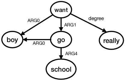
Figure 1: AMR Graph for the Sentence: The boy really wants to go to school.

AMR parsing is the task that maps a sentence to an AMR semantic graph automatically. A graph is a complex data structure which is composed of multiple vertices and edges. To produce a graph, one must determine the order of producing these vertices and edges. There are roughly four kinds of orders in previous work:

• Two-Stage Order (Flanigan et al., 2014; Lyu and Titov, 2018; Zhang et al., 2019a; Zhou et al., 2020): first produce vertices, and produce edges after that.

• Transition-Based Order (Damonte et al., 2016; Ballesteros and Al-Onaizan, 2017; Guo and Lu, 2018; Wang and Xue, 2017; Naseem et al., 2019): process the sentence from left to right, and produce vertices and edges based on the current focused word.

• Depth-first Based Order (Konstas et al., 2017; van Noord and Bos, 2017; Peng et al., 2017, 2018; Zhang et al., 2019b): produce vertices and edges based on depth-first order.

• Breadth-first Based Order (Cai and Lam, 2019, 2020): produce vertices based on breadth-first order, and produce edges between the new vertex and existing vertices when producing each vertex.

We focus on the last type — breath-first based order, which was proposed by Cai and Lam and achieves better performance than other strategies. In this order, vertices and edges that are close to the root vertex are produced first. In AMR, these vertices usually capture the core semantics of a sentence. Therefore, models in this order pay more attention to the core semantics, which is one reason that they usually show better performance.

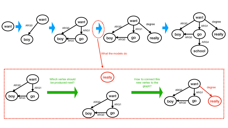
Figure 2: How previous methods generate the AMR graph in the breadth-first way for the sentence: The boy really wants to go to school.

However, the existing breadth-first based methods (Cai and Lam, 2019, 2020) are not truly breadth-first. They only encourage the model to produce the AMR graph in the breadth-first way, but cannot guarantee this. To see this, we first show how they generate the AMR graph in Figure 2. Each time they update the graph, they first produce a new vertex (the vertex really in this example), then they connect this new vertex to its parents (the edge degree in this example). There is no guarantee that the new vertex is produced in the breadth-first order. For example, in Figure 3, the models may incorrectly produce a second-layer child vertex school before producing the last first-layer child vertex really. While they cannot guarantee the breadth-first order, they achieve it in most steps in the parsing. This is because they encourage this order during training by always choosing the gold next-child in breadth-first order, shown also in Figure 3.

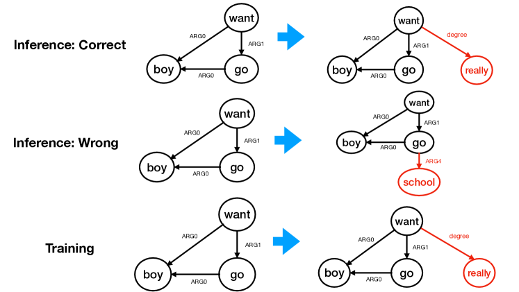
Figure 3: No guarantee of the breadth-first order for inference. Training process encourages the breadth-first order by always choosing the gold next-child in this order.

In this paper, we design a new architecture such that the AMR graph is guaranteed to be generated in the breadth-first order. In each step, we introduce a focused parent vertex, and produce the next child for this parent vertex. We will not change this focused parent until we have produced all its children. After producing all its children, we change the focused parent to be the next in breadth-first order, guaranteeing that the graph is generated in the desired order.

For example, in Figure 4, we show the entire flow of producing the AMR graph for the sentence The boy really wants to go to school. We first produce the root vertex want (step 1), and label this root vertex as the focused parent vertex. Then we produce the three child vertices of the root vertex: boy, go, and really (steps 2, 3, 4). In step 5, we find that the root vertex want has no remaining children, so we shift our focus parent from want to its first child boy. In step 6, we find that boy has no child, so we shift the focused parent from boy to its sibling go. In steps 7 and 8, we produce the two children of go. One child is a new vertex school, and the other is an existing vertex boy. After that, we shift the focused parent to the last child of root vertex want in step 9, but find no child of it in step 10. At this point, we have finished dealing with all the first-layer children. In step 11, we find there is no child of the only second-layer child school. Therefore, we finish the whole parsing.

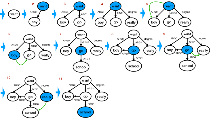
Figure 4: AMR Graph Producing Flow for Sentence: The boy really wants to go to school. Here, the green arrows shows the shift of the focused parent vertex.

The contributions of our works are summarized as follows:

• We propose a new AMR parsing architecture that strictly follows the breadth-first order to generate the AMR graph. In each step, we introduce a focused parent vertex to guide the construction.

• We improve the encoding part for the sentence and the partial graph by using a new BERT Based Embedding Layer (Section 3.1.1) and adding edge information (Section 3.2.3). We demonstrate their effectiveness in Section 5.3.

• Our model achieves better performance than Cai and Lam on both the AMR 1.0 dataset and the AMR 2.0 dataset.

2 Some Concepts in Sentence and Graph

In this section, we give some explanations about the vertices and edges in the graph under our definition. We divide every vertex and edge into several parts and will process or predict these parts separately in our model. In Figure 5a, we show an AMR from our dataset and translate it into a graph in Figure 5b before these processing steps. We show the graph after these processing steps in Figure 5c.

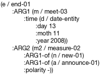
(a) AMR from dataset

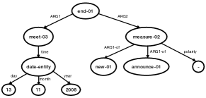
(b) AMR graph before processed

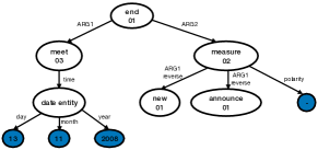
(c) AMR graph after processed

Figure 5: AMR graph preprocess for the sentence: The 081113 meeting ended without any new measures to announce. Notice that we show the type part by the color. Blue vertices mean attribute vertices, and white vertices mean instance vertices

2.1 Vertex

We divide every vertex into three parts: type, sense and content.

Type

There are two types for each vertex, and we call them instance and attribute. We can see this in Figure 5a. In that AMR, some vertices are preceded by some variables, like e / end-01 (variable e), d / date-entity (variable d), and n / new-01 (variable n). These vertices are of type instance. The others do not have a preceding variable, like 13, 2008. These vertices are of type attribute.

Intuitively, an instance is produced according to the meaning of a word or a phrase from the sentence, usually not a direct copy of some word (but sometimes is a copy from the lemma of this word). Some special instances do not occur in the sentence, like date-entity in Figure 5a.

An attribute represents some property of its parent. For example, a name instance vertex usually has attributes each representing one word of the name. In the example of Figure 5a, 13, 11, and 2008 are the exact day, month, and year property of their parent, date-entity. If an attribute occurs in the sentence, it is usually the same as some word in the sentence. But there are some attributes that are not the copy of words, like the negative property ‘-’ in this example.

Content and sense

Some instances end with some number called sense. The same word with different sense has different meanings. We separate an instance into content and sense (if present), by the dash. In Figure 5a, for example, end-01 is separated into end and 01.

Furthermore, in an instance, if its content is composed of more than one word, these words are usually connected with a hyphen, like date-entity. We separate an instance by hyphens into several words.

2.2 Edge

We divide the edge label into two parts: label and if-reverse.

Some edges in the AMR graph end with -of. They represent the reverse relation. For example, in Figure 5a, measure-02 has a child new-01 with edge ARG1-of. The sequential reading is that the ARG1-of branch of measure-02 is new-01, but the graph interpretation is that the ARG1 branch of new-01 is measure-02.

If an edge ends with -of, we say this label’s if-reverse part is true, otherwise it is false. The left part in this edge is called its label.

3 Model Architecture

In this section, we describe the details of our model. Given the source sentence, the partial graph and the focused parent, the model produces the next child node of this focused parent (step 3 in Figure 4) or change the focused parent (step 5 in Figure 4).

Our model consists of four parts: Sentence Encoder, Partial Graph Encoder, Interactive Module and Prediction Module. The Sentence Encoder and Partial Graph Encoder separately encode the source sentence and the partial graph into some hidden vectors. The Interactive Module exchanges the information from the sentence and the partial graph with each other. The Prediction Module uses the exchanged information to make necessary predictions to build the next child or change the focused parent.

For the following discussion, let us assume that the source sentence is denoted by $w_{1},w_{2},\ldots,w_{m}$, where $w_{i}$ ($1\leq i\leq m$) denotes the $i$th token in the sentence. The partial graph is denoted by $v_{1},v_{2},\ldots,v_{t}$, where $v_{j}$ ($1\leq j\leq t$) denotes the $j$th node in the partial graph. If $v_{i}$ has $v_{j}$ as its child, we use $e_{i,j}$ to denote the edge from $v_{i}$ to $v_{j}$, and also use $e_{j,i}$ to denote the reverse edge of $e_{i,j}$ (add or remove the suffix -of). We use $\mathscr{E}_{i}$ to denote the set of edges that point to all the children and parents (in-neighbours and out-neighbours) of $v_{i}$.

3.1 Sentence Encoder

We encode the sentence $w_{1},w_{2},\ldots,w_{m}$ into hidden vectors $\bm{h}_{0},\bm{h}_{1},\bm{h}_{2},\ldots,\bm{h}_{m}$ in this part. Note that there is one more vector $\bm{h}_{0}$, which is used to summarize the sentence and for the prediction module. To perform the encoding, we first compute the embedding vector $\bm{e}_{i}$ for each token $w_{i}$ in the sentence. Then we use $\{\bm{e}_{i}\}_{i=1}^{m}$ to compute the encoding vectors $\{\bm{h}_{i}\}_{i=0}^{m}$.

3.1.1 Embedding Vectors for the Sentence

We use a framework similar to Cai and Lam (2020) for this part. In that paper, they computed five vectors for every token in the sentence, corresponding to the lemma $\bm{l}_{i}$, token itself $\bm{t}_{i}$, part-of-speech $\bm{p}_{i}$, named entity tag $\bm{n}_{i}$ and BERT feature $\bm{b}_{i}$, then combined these five vectors as the final embedding vector $\bm{e}_{i}$.

They run BERT for the input sentence and used the vectors of the top layer to construct the BERT feature $\bm{b}$. Since BERT is computed on sub-tokens instead of tokens of the sentence, they first computed BERT encoding vectors on sub-tokens of the sentence, then averaged the vectors of the sub-tokens within each token as the final vector of BERT feature. For the remaining four embedding vectors $\bm{l},\bm{t},\bm{p}$ and $\bm{n}$, they used four learned embedding layers to compute them.

Here, we use the same BERT feature $\bm{b}$ to summarize the information of the whole sentence. We also similarly use two learned embedding layers for part-of-speech $\bm{p}$ and name entity tag $\bm{n}$. But for the token $\bm{t}$ and lemma $\bm{n}$, we design an improved embedding layer called BERT Based Embedding Layer.

BERT Based Embedding Layer

The reason to use a different method for the token and lemma is that they are words, not just a label like part-of-speech and name entity tag. The naive embedding layer in Cai and Lam (2020) used randomly initialized learned vectors for every word (token and lemma). However, we want to leverage the powerful pretrained model — BERT — to encode the word, even though BERT is originally designed to encode the sentence, not a single word. Therefore, we construct the final embedding vector using the sum of the BERT vector and a learned refinement embedding vector. The refinement embedding vector is used to adjust BERT to fit our specific AMR parsing task. Specifically, suppose we want to find the embedding vector for word $w$, and the BERT sub-tokenization for $w$ is $s_{1},s_{2},\ldots,s_{u}$. We use BERT to compute the encoding vector $\bm{s}_{1},\bm{s}_{2},\ldots,\bm{s}_{u}$ for each sub-token, then we compute the final BERT based embedding vector as follows:

$$\bm{w}^{\textrm{BERT}} = \sum_{i=1}^{u}\bm{s}_{i}/u,$$ (1)

$$\bm{w}^{\textrm{Final}} = W^{T}\left(a\left(W^{B}\bm{w}^{\textrm{BERT}}+\textrm{Emb}\left(w\right)\right)\right),$$

where $\bm{w}^{\textrm{BERT}}\in\mathbb{R}^{b},\bm{w}^{\textrm{Final}}\in\mathbb{R}^{g},W^{B}\in\mathbb{R}^{e\times b},W^{T}\in\mathbb{R}^{g\times e}$, $a(\cdot)$ is the activation function and $\textrm{Emb}(\cdot)$ is the learnt refinement embedding layer. Here, $b$ is the length for BERT encoding vector, $e$ is the size for refinement embedding vector, $g$ is graph size, which will be the same as the length of graph encoding vectors and $u$ is the number of sub-tokens in word $w$. Here, we let $e$ be smaller than $b$ since we think the main part of embedding is still from BERT.

BERT Based Embedding Layer is used to compute the word embeddings, like token embedding $\bm{t}$ and lemma embedding $\bm{l}$. It is different from the BERT feature embedding vector $\bm{b}$ (remember that we have five different embedding parts: token, lemma, part-of-speech, name entity tagging and BERT feature). For the BERT feature $\bm{b}$, we compute the vectors based the whole sentence information, but the BERT Based Embedding Layer only considers the word itself. Note that our model still uses the BERT feature $\bm{b}$ to summarize the information of the whole sentence.

3.1.2 Sentence Encoding

We insert a special embedding $\bm{e}_{0}$ at the beginning of the sentence in order to summarize the sentence later. Now, the sequence embedding vectors become $\{\bm{e}_{i}\}_{i=0}^{m}$. We then employ $L_{S}$ Transformer Encoder Layers to encode the sentence. We denote the final sentence encoding vector by $\{\bm{h}_{i}\}_{i=0}^{m}$.

3.2 Partial Graph Encoder

Suppose now we have $t$ vertices in the partial graph, denoted by $v_{1},v_{2},\ldots,v_{t}$, and some edges between them denoted by $\{e_{i,j}\}$ (in the beginning of Section 3 we mentioned that we have added the reverse edge for every edge). We will encode this partial graph into $t+1$ hidden vectors $\{\bm{g}_{i}\}_{i=0}^{t}$ in this part, where each hidden vector $\bm{g}_{i}$ denotes the vertex $v_{i}$ and the information about its descendants and ancestors, and we will also insert a special encoding vector $\bm{g}_{0}$ as in the sentence encoding.

To do this, we first compute vertex and edge embedding vectors $\bm{v}_{i}$ and $\bm{e}_{i,j}$ for each vertex $v_{i}$ and edge $e_{i,j}$. Then we use a Graph Recurrent Network to gradually collect information about the descendants’ and ancestors’ information.

3.2.1 Vertex Embedding

In Section 2.1, we mentioned that a vertex is composed of three parts: type, content, and sense. Here, we only use content information for graph encoding.

For illustration, we consider the instance vertex go-back-19. As we discussed in Section 2, the content of this node is go back. We use BERT Based Embedding Layer to compute the content embedding $\bm{v}_{i}$. Here, even though there are two words in go back, we are still able to use BERT Based Embedding Layer since the sub-token algorithm in BERT can also be used on phrases, and for the refinement part, we can treat the phrase as a whole unit and assign an embedding vector for this unit.

3.2.2 Edge Embedding

For the edge $e_{i,j}$, as we introduced in Section 2.2, it is composed of the label part and if-reverse part. We use two naive embedding layers to separately compute their embeddings $\bm{e}_{i,j}^{\textrm{label}}$ and $\bm{e}_{i,j}^{\textrm{reverse}}$, and compute their sum as the total edge embedding $\bm{e}_{i,j}$.

3.2.3 Graph Encoding

Having the embeddings of all the vertices and edges, we are able to encode this partial graph. We construct the graph encoding repeatedly by gradually collecting the information about the descendants and ancestors for every vertex. Formally, we repeat the following recurrence for $L_{G}$ times:

$$\bm{v}_{i}^{l,0}= \textrm{LN}\left(\bm{v}_{i}^{l-1,1}+\sum_{j\in\mathscr{E}_{i}}W^{l}[\bm{v}_{j}^{l-1,1};\bm{e}_{i,j}]/|\mathscr{E}_{i}|\right),$$

$$\bm{v}_{i}^{l,1}= \textrm{LN}\left(\bm{v}_{i}^{l,0}+\textrm{FFN}^{l}\left(\bm{v}_{i}^{l,0}\right)\right),$$

where LN represents layer normalization layer and FFN denotes feed-forward layer, and $\bm{v}_{i}^{0,1}=\bm{v}_{i}$. We use the output of the last layer $\{\bm{v}_{i}^{L_{G},1}\}_{i=1}^{t}$ as the graph encoding result, and we denote them by $\{\bm{g}_{i}\}_{i=1}^{t}$. Then, as we did for the sentence encoding, we insert a special encoding vector $\bm{g}_{0}$.

Different from Cai and Lam (2020), we add edge information here. We will demonstrate its effectiveness in Section 5.3.

3.3 Interactive Module

After we obtain the sentence encoding vectors $\{\bm{h}_{i}\}_{i=0}^{m}$ and partial graph encoding vectors $\{\bm{g}_{i}\}_{i=0}^{t}$, we want to exchange these pieces of information and prepare a vector for the Prediction Module. We also include the information about the focused parent in this module. Suppose the focused parent is $v_{\textrm{focus}}$ and its encoding vector is $\bm{g}_{\textrm{focus}}$. We design an interactive Transformer layer to let them interact with each other.

Interactive Transformer Layer

Specifically, in the $l$th interactive Transformer layer, we first add weighted sentence information to each graph vertex:

$$\bm{g}_{i}^{l,0} =\textrm{LN}\left(\bm{g}_{i}^{l-1,2}+\textrm{Attn}^{l,S,0}\left(\bm{g}_{i}^{l-1,2},\bm{h}_{0:m}^{l-1,3}\right)\right),$$

$$\bm{g}_{i}^{l,1} =\textrm{LN}\left(\bm{g}_{i}^{l,0}+\textrm{Attn}^{l,S,1}\left(\bm{g}_{i}^{l,0},\bm{g}_{0:t}^{l,0}\right)\right),$$

$$\bm{g}_{i}^{l,2} =\textrm{LN}\left(\bm{g}_{i}^{l,1}+\textrm{FFN}^{l,S}\left(\bm{g}_{i}^{l,1}\right)\right),$$

where $\bm{h}_{i}^{0,3}=\bm{h}_{i}$, and $\bm{g}_{i}^{0,2}=\bm{g}_{i}$. Then, we add weighted graph vertex information to each sentence node. We also add the focused parent information here:

$$\bm{h}_{i}^{l,0} =\textrm{LN}\left(\bm{h}_{i}^{l-1,3}+\textrm{Attn}^{l,G,0}\left(\bm{h}_{i}^{l-1,3},\bm{g}_{0:t}^{l,2}\right)\right),$$

$$\bm{h}_{i}^{l,1} =\textrm{LN}\left(\bm{h}_{i}^{l,0}+\bm{g}_{\textrm{focus}}\right),$$

$$\bm{h}_{i}^{l,2} =\textrm{LN}\left(\bm{h}_{i}^{l,1}+\textrm{Attn}^{l,G,1}\left(\bm{h}_{i}^{l,1},\bm{h}_{0:m}^{l,1}\right)\right),$$

$$\bm{h}_{i}^{l,3} =\textrm{LN}\left(\bm{h}_{i}^{l,2}+\textrm{FFN}^{l,G}\left(\bm{h}_{i}^{l,2}\right)\right).$$

We apply $L_{I}$ interactive Transformer layers. We use the first vector of the sentence in the top layer $\bm{h}_{0}^{L_{I},3}$ for prediction and we denote it by $\bm{h}^{p}$. Also, we will use $\{\bm{g}_{i}^{L_{I},2}\}_{i=1}^{t}$ in the Prediction Module as well, and we denote them by $\{\bm{g}_{i}^{p}\}_{i=1}^{t}$.

3.4 Prediction Module

Finally, we come to the prediction part. First, we use $\bm{h}^{p}$ (obtained in Interactive module) to predict if there is another child for the focused parent. If there is no other child, we will change the focused parent. Otherwise, we will produce the vertex and edge of the next child.

We first predict the vertex, then predict the edge based on the predicted vertex. If the next child is a vertex produced previously, we will use $\bm{h}^{p}$ and the information of all produced vertices $\{\bm{g}_{i}^{p}\}_{i=1}^{t}$ (obtained in the Interactive module) to predict it. If the next vertex is a new instance or attribute, we will use $\bm{h}^{p}$ to predict the content and sense of the new vertex. Like Cai and Lam (2020), the prediction of the content can be either producing a new content from content vocabulary or copying of some word in sentence.

After predicting the vertex, we use it together with $\bm{h}^{p}$ to predict the new edge. Like the vertex, we separately predict the label part and if-reverse part of the edge.

The details of this Prediction Module are provided in Appendix A.

4 Training and Inference

4.1 Training

We use the standard maximum likelihood method to train the model. The loss function for one data point (input sentence with gold graph) is the sum of the negative log-likelihood for every partial graph corresponding to the gold graph, where the negative log-likelihood for each partial graph is again the sum of all the components introduced in Section 3.4 (and Appendix A for details). We use breadth-first order to break the gold graph into several incremental partial graphs. But for each parent, there is still more than one order to produce its children. Following Cai and Lam (2020), with 0.5 probability we use a deterministic order (sorted by the frequency of edge labels), and with 0.5 probability we use a uniformly random order.

4.2 Inference

Since our model is auto-regressive (it produces a new vertex and edge based on previous partial graphs and in each partial graph predicts a new object based on previous predicted objects, see Section 3.4), we use beam search to produce the whole graph.

5 Experiments

5.1 Setup

Dataset

We evaluate our model on the AMR 1.0 (LDC2014T12) and AMR 2.0 (LDC0217T10) datasets. AMR 1.0 contains 13051 sentences in total while AMR 2.0 has about 39000. Both datasets have already been split into training, development and testing parts. Since AMR 2.0 is larger, we use it as our main dataset.

Implementation Detail

We use Stanford CoreNLP (Manning et al., 2014) to obtain the token, lemma, part-of-speech and named-entity tagging for each word in the sentence (Section 3.1). We use pre-trained models in Devlin et al. (2019) to compute BERT vectors.

We employ similar pre-processing and post-processing steps to Cai and Lam (2020). For the pre-processing step, we also break the vertex and the edge into several parts as described in Section 2. For the post-processing, we also employ the reverse operations of pre-processing operations, combining the several components into a whole unit for the vertex and the edge.

During training, we fix the BERT parameters similar to Cai and Lam (2020) due to GPU limitation (and we add the learned refinement term in BERT Based Embedding Layer for compensation). We use ADAM optimization with decayed learning rate similar to Vaswani et al. (2017) to train the model. Training takes approximately 7 hours on four Nvidia GeForce GTX 1080 Ti.

We use development data to tune the hyper-parameters. The hyper-parameters we used in our best model are described in Appendix B. We use a beam size of 8 to produce the graph.

model	G.R.	Smatch	Unlabeled	NO WSD	Concept	SRL	Reent.	Neg.	NER	wiki
Groschwitz et al. (2018)	$\checkmark$	71.0	74	72	84	64	49	57	78	71
Lyu and Titov (2018)	$\checkmark$	74.4	77.1	75.5	85.9	69.8	52.3	58.4	86.0	75.7
Lindemann et al. (2019)	$\checkmark$	75.3	-	-	-	-	-	-	-	-
Naseem et al. (2019)	$\checkmark$	75.5	80	76	86	72	56	67	83	80
Zhang et al. (2019a)	$\checkmark$	76.3	79.0	76.8	84.8	69.7	60.0	75.2	77.9	85.8
Zhang et al. (2019b)	$\checkmark$	77.0	80	78	86	71	61	77	79	86
Zhou et al. (2020)	$\checkmark$	77.5	80.4	78.2	85.9	71.0	61.1	76.1	78.8	86.5
Cai and Lam (2020)	$\checkmark$	80.2	82.8	80.8	88.1	74.2	64.6	78.9	81.1	86.3
Ours	$\checkmark$	81.1	84.0	81.9	87.3	74.9	67.7	76.7	80.4	86.9

Table 1: Overall Smatch scores and fine-grained scores of different parsers on AMR 2.0 dataset. Some results of previous models come from Cai and Lam (2020). Here, G.R. means graph re-categorization. All the models in this table include the re-categorization process.

5.2 Results

Main Results

We show our main results in Table 1. This includes the overall Smatch score and fine-grained scores (Damonte et al., 2017) of our model and previous models on the AMR 2.0 dataset. We can see that our model beats Cai and Lam by 0.9% and is better for the most of the fine-grained scores.

Results for Models without Re-categorization

Most of the AMR parsing models include a complex pre-processing step called re-categorization. With re-categorization, specific sub-graphs of a AMR graph (usually corresponding to special entities, like named entities, date entities, etc.) are treated as a unit and assigned to a single vertex with a new content. The re-categorization process is composed of several hand-crafted rules, requiring exhaustive screening and expert-level manual efforts. This is a feasible idea for the current dataset since the dataset is small (about 40000 sentences in AMR 2.0 dataset). However, when the dataset becomes larger in the future, using machine learning to automatically learn a model will be a better idea than hand-crafted rules.

Therefore, we want to see the performance of our model without re-categorization and we show the result in Table 2. Our model beats Cai and Lam by 1.3% and is above 80% for the first time. Also, our model is better for most of the fine-grained scores.

model	G.R.	Smatch	Unlabeled	NO WSD	Concept	SRL	Reent.	Neg.	NER	wiki
van Noord and Bos (2017)	$\times$	71.0	74	72	82	66	52	62	79	65
Cai and Lam (2019)	$\times$	73.2	77.0	74.2	84.4	66.7	55.3	62.9	82.0	73.2
Cai and Lam (2020)	$\times$	78.7	81.5	79.2	88.1	74.5	63.8	66.1	87.1	81.3
Ours	$\times$	80.0	83.1	80.8	87.4	75.6	67.5	62.5	87.5	79.7

Table 2: Overall Smatch scores and fine-grained scores of different parsers on AMR 2.0 dataset. Some results of previous models come from Cai and Lam (2020). Here, G.R. means graph re-categorization. All the models in this table do not include the re-categorization process.

Results for AMR 1.0 Dataset

Next we evaluate our model on the AMR 1.0 dataset. We show the results in Table 3 for models with the re-categorization pre-processing step and show the results in Table 4 for models without the re-categorization pre-processing step. We can see that our model beats every previous model for both situations.

model	G.R.	Smatch
Wang and Xue (2017)	$\checkmark$	68.1
Guo and Lu (2018)	$\checkmark$	68.3
Zhang et al. (2019a)	$\checkmark$	70.2
Zhang et al. (2019b)	$\checkmark$	71.3
Cai and Lam (2020)	$\checkmark$	75.4
Ours	$\checkmark$	75.8

Table 3: Smatch scores of different models with the re-categarization pre-processing step on AMR 1.0 dataset. Some results of previous models come from Cai and Lam (2020).

model	G.R.	Smatch
Flanigan et al. (2014)	$\times$	66.0
Pust et al. (2015)	$\times$	67.1
Cai and Lam (2020)	$\times$	74.0
Ours	$\times$	74.6

Table 4: Smatch scores of different models without the re-categarization pre-processing step on AMR 1.0 dataset. Some results of previous models come from Cai and Lam (2020).

model	Smatch
with edge	81.1
without edge	80.8

Table 5: The effect of edge information.

model	Smatch
our model	81.1
remove BERT	80.7

Table 6: Effect of BERT for BERT Based Embedding Layer.

5.3 Ablation Study

Effect of Edge Information

In the previous SOTA model (Cai and Lam, 2020), they did not add edge information in Graph Encoder part. They claimed that the edge information had little influence on the performance of their model. Therefore, we want to see if edge information is important in our model. We evaluate it on AMR 2.0 dataset. From Table 5, we see that the Smatch score of our model with edge information is higher than the score without edge information. This demonstrates that the edge information is helpful in our model.

Effect of BERT Based Embedding Layer

In our model, we introduce a new embedding layer named BERT Based Embedding Layer to better encode the tokens, lemmas (Section 3.1.1) and vertices (Section 3.2.1). However, in the previous SOTA model (Cai and Lam, 2020), they only use learnt embedding layers for them, which means they did not include a BERT component (Equation (1)) for those words (but they still run the BERT for the whole sentence to construct the BERT feature $\bm{b}$ mentioned in Section 3.1.1). So we want to see its effect in our model. In Table 6, we can see that when removing the BERT part, the Smatch score decreases by 0.4%, which demonstrates that BERT plays an important role here.

6 Conclusion

In this paper, we propose a new AMR parsing architecture that strictly follows the breadth-first order to generate the AMR graph. With the help of the focused parent information, a better word embedding layer named BERT Based Embedding Layer and the edge information in graph encoding, our model is able to construct the AMR more accurately. Our model achieves better performance on the both AMR 1.0 and AMR 2.0 datasets.

Acknowledgments

Research supported by NSF awards IIS-1813823 and CCF-1934962.

Appendix A Details of Prediction Module

As we discussed in Section 3.4, we first predict the vertex, then predict the edge based on the predicted vertex (if it exists).

A.1 Predict Vertex

There are four situations about the next vertex (we give each situation a label for classification):

1. there is no other child (label 0);

2. the next vertex is a node produced previously (label 1);

3. the next vertex is a new instance (label 2);

4. the next vertex is a new attribute (label 3).

We must predict the situation before any further prediction. We use $\bm{o}$ to denote the status and use $\bm{h}^{p}$ to predict the status $\bm{o}$:

$$p(\bm{o})=\textrm{Softmax}\left(W^{o}\bm{h}^{p}+\bm{b}^{o}\right).$$

Now we make further prediction based on $\bm{o}$.

No Other Child ($\bm{o}=0$)

This means there are no other children, so we will change the focused parent, like the step 5 in Figure 4.

Previously Produced ($\bm{o}=1$)

This means the next child is some vertex produced previously. We compute the probability vector using an Attention layer:

$$p_{1:t}^{r}=\textrm{Softmax}\left(\left(W^{r,0}\bm{h}^{p}\right)^{\top}W^{r,1}\bm{g}_{1:t}^{p}\right).$$

We use $v^{r}$ to denote the index of the produced vertex that the next child equals, then we have $p\left(v^{r}\right)=p_{v^{r}}^{r}$.

New Instance ($\bm{o}=2$)

This means the next vertex is of type instance. Then we must predict its content and sense. But before that, we use a simple linear layer to transfer $\bm{h}^{p}$ into instance mode $\bm{h}^{\textrm{conc}}$:

$$\bm{h}^{\textrm{conc}}=\bm{h}^{p}+a\left(W^{\textrm{conc}}\bm{h}^{p}\right),$$

We divide the prediction of content into two parts. In the first part, we think the content is a new word or a new phrase, not directly copied from any word in the sentence, such as date-entity. In the second part, we think the content comes directly from the sentence. We use a soft linear layer to predict this:

$$[p_{0},p_{1}]=\textrm{Softmax}\left(W^{s}\bm{h}^{\textrm{conc}}+\bm{b}^{s}\right).$$

Now, suppose we denote the predicted content by $c$. In the first part, we use linear and softmax layer to predict it from content vocabulary:

$$p^{\textrm{new}}(c)=\textrm{Softmax}(W^{\textrm{new}}\bm{h}^{\textrm{conc}}+\bm{b}^{\textrm{new}}).$$

In the second part, we think the content comes from some word (more precisely, the lemma of the word) of the sentence, so we use Attention layer to predict the probability vector:

$$p_{1:m}^{\textrm{lemma}}=\textrm{Softmax}\left(\left(\bm{h}^{\textrm{conc}}\right)^{\top}\bm{l}_{1:m}\right),$$

where $\bm{l}_{1:m}$ are the embedding vectors of lemmas which are introduced in Section 3.1. The final probability of the predicted content $c$ is:

$$p(c)=p_{0}p^{\textrm{newc}}(c)+p_{1}\sum_{i:l_{i}=c}p_{i}^{\textrm{lemma}}.$$

Once we predict the content, we use BERT Based Embedding Layer to obtain the embedding vector $\bm{c}$. Then we are able to predict the sense of this vertex. We use $s$ to denote the sense and compute the probability as follows:

$$p(s)=\textrm{Softmax}\left(W^{\textrm{sense}}\left[\bm{h}^{\textrm{conc}};\bm{c}\right]+\bm{b}^{\textrm{sense}}\right).$$

New Attribute ($\bm{o}=3$)

This means the next vertex is of type attribute. Notice that an attribute does not have a sense, so we only have to predict its content. Similar to instance, we first transfer $\bm{h}^{p}$ into attribute mode $\bm{h}^{\textrm{attr}}$:

$$\bm{h}^{\textrm{attr}}=\bm{h}^{p}+a\left(W^{\textrm{attr}}\bm{h}^{p}\right).$$

Then we divide the prediction of attribute into two parts. One is a new word and the other is directly copying from some word in the sentence. Similar to instance, we use the same soft linear layer to predict the phase:

$$[p_{0},p_{1}]=\textrm{Softmax}\left(W^{s}\bm{h}^{\textrm{attr}}+\bm{b}^{s}\right).$$

Suppose we denote the predicted attribute by $a$. In the first part, we also use the same soft linear layer to predict it from content vocabulary:

$$p^{\textrm{new}}(a)=\textrm{Softmax}(W^{\textrm{new}}\bm{h}^{\textrm{attr}}+\bm{b}^{\textrm{new}}).$$

In the second part, different from instance, we think the content comes from the token instead of the lemma of some word in sentence, so we have:

$$p_{1:m}^{\textrm{token}}=\textrm{Softmax}\left(\left(\bm{h}^{\textrm{attr}}\right)^{\top}\bm{t}_{1:m}\right),$$

where $\bm{t}_{1:m}$ are the embedding vectors of tokens which are introduced in Section 3.1. The final probability of the predicted content $c$ is:

$$p(a)=p_{0}p^{\textrm{new}}(a)+p_{1}\sum_{i:w_{i}=a}p_{i}^{\textrm{token}}.$$

A.2 Predict Edge

The last thing we will predict is the edge (if $\bm{o}\not=0$). We need to predict the label part and the if-reverse part. But before that, we need to produce a vector to represent the predicted vertex since we also need to use the vertex information here. There are two situations here:

• previously-produced vertex: in this situation, we use the corresponding graph encoding vector to represent it. Suppose this previously-produced vertex is $v_{i}$, then we use $\bm{g}_{i}^{p}$;

• new instance or attribute: in this situation, we use the method in Section 3.2.1 to compute the vector.

Anyway, we use $\bm{v}^{\textrm{predict}}$ to denote this vector.

Now we are able to predict the edge. First, we predict the label part and we denote it by $e^{l}$:

$$p(e^{l})=\textrm{Softmax}\left(W^{e,l}\left[\bm{h}^{p};\bm{v}^{\textrm{predict}}\right]+\bm{b}^{e,l}\right).$$

Then, we use the edge embedding layer introduced in Section 3.2.2 to get the embedding vector $\bm{e}^{l}$ for it.

After that, we predict the if-reverse part and we denote it by $e^{r}$:

$$p(e^{r})=\textrm{Softmax}\left(W^{e,r}\left[\bm{h}^{p};\bm{v}^{\textrm{predict}};\bm{e}^{l}\right]+\bm{b}^{e,r}\right).$$

Appendix B Hyper-Parameters

We use PyTorch for all the experiments. We try different sizes for the hidden vectors and embedding vectors from 128 to 1024 (128, 256, 512, 1024), and try different number of layers from 2 to 8. We use the Smatch score of the validation data to perform the hyperparameter selection. We show hyper-parameters of our best model in Table 7. Here, graph hidden size represents the size of all the embedding vectors (excluding the BERT vectors and refinement vectors, but they will finally be transformed to the graph hidden size, see Section 3.1.1), sentence encoding vectors, graph encoding vectors.

refinement embedding size	300
graph hidden size	512
graph encoding layers	4
sentence encoding layers	4
interactive Transformer layers	4
Transformer feed-forward hidden size	1024
number of Transformer heads	8
dropout	0.1
beam size	8

Table 7: Hyper-parameters

References

- Ballesteros and Al-Onaizan (2017) Miguel Ballesteros and Yaser Al-Onaizan. 2017. AMR parsing using stack-LSTMs. In Proceedings of the 2017 Conference on Empirical Methods in Natural Language Processing, pages 1269–1275.
- Banarescu et al. (2013) Laura Banarescu, Claire Bonial, Shu Cai, Madalina Georgescu, Kira Griffitt, Ulf Hermjakob, Kevin Knight, Philipp Koehn, Martha Palmer, and Nathan Schneider. 2013. Abstract meaning representation for sembanking. In Proceedings of the 7th Linguistic Annotation Workshop and Interoperability with Discourse, pages 178–186, Sofia, Bulgaria.
- Cai and Lam (2019) Deng Cai and Wai Lam. 2019. Core semantic first: A top-down approach for AMR parsing. In Proceedings of the 2019 Conference on Empirical Methods in Natural Language Processing and the 9th International Joint Conference on Natural Language Processing (EMNLP-IJCNLP), pages 3790–3800.
- Cai and Lam (2020) Deng Cai and Wai Lam. 2020. AMR parsing via graph-sequence iterative inference. In Proceedings of the 58th Annual Meeting of the Association for Computational Linguistics, pages 1290–1301, Online. Association for Computational Linguistics.
- Damonte et al. (2016) Marco Damonte, Shay B. Cohen, and Giorgio Satta. 2016. An incremental parser for abstract meaning representation. CoRR, abs/1608.06111.
- Damonte et al. (2017) Marco Damonte, Shay B. Cohen, and Giorgio Satta. 2017. An incremental parser for abstract meaning representation. In Proceedings of the 15th Conference of the European Chapter of the Association for Computational Linguistics (EACL), pages 536–546, Valencia, Spain.
- Devlin et al. (2019) Jacob Devlin, Ming-Wei Chang, Kenton Lee, and Kristina Toutanova. 2019. BERT: Pre-training of deep bidirectional transformers for language understanding. In Proceedings of the 2019 Conference of the North American Chapter of the Association for Computational Linguistics: Human Language Technologies, Volume 1 (Long and Short Papers), pages 4171–4186.
- Flanigan et al. (2014) Jeffrey Flanigan, Sam Thomson, Jaime Carbonell, Chris Dyer, and Noah A. Smith. 2014. A discriminative graph-based parser for the abstract meaning representation. In Proceedings of the 52nd Annual Meeting of the Association for Computational Linguistics (ACL-14), pages 1426–1436, Baltimore, Maryland.
- Groschwitz et al. (2018) Jonas Groschwitz, Matthias Lindemann, Meaghan Fowlie, Mark Johnson, and Alexander Koller. 2018. AMR dependency parsing with a typed semantic algebra. In Proceedings of the 56th Annual Meeting of the Association for Computational Linguistics (Volume 1: Long Papers), pages 1831–1841. Association for Computational Linguistics.
- Guo and Lu (2018) Zhijiang Guo and Wei Lu. 2018. Better transition-based AMR parsing with a refined search space. In Proceedings of the 2018 Conference on Empirical Methods in Natural Language Processing, pages 1712–1722, Brussels, Belgium. Association for Computational Linguistics.
- Hardy and Vlachos (2018) Hardy Hardy and Andreas Vlachos. 2018. Guided neural language generation for abstractive summarization using abstract meaning representation. In Proceedings of the 2018 Conference on Empirical Methods in Natural Language Processing, pages 768–773.
- Konstas et al. (2017) Ioannis Konstas, Srinivasan Iyer, Mark Yatskar, Yejin Choi, and Luke Zettlemoyer. 2017. Neural AMR: Sequence-to-sequence models for parsing and generation. In Proceedings of the 55th Annual Meeting of the Association for Computational Linguistics (Volume 1: Long Papers), pages 146–157, Vancouver, Canada. Association for Computational Linguistics.
- Lindemann et al. (2019) Matthias Lindemann, Jonas Groschwitz, and Alexander Koller. 2019. Compositional semantic parsing across graphbanks. In Proceedings of the 57th Annual Meeting of the Association for Computational Linguistics, pages 4576–4585, Florence, Italy. Association for Computational Linguistics.
- Liu et al. (2015) Fei Liu, Jeffrey Flanigan, Sam Thomson, Norman Sadeh, and Noah A. Smith. 2015. Toward abstractive summarization using semantic representations. In Proceedings of the 2015 Conference of the North American Chapter of the Association for Computational Linguistics: Human Language Technologies, pages 1077–1086.
- Lyu and Titov (2018) Chunchuan Lyu and Ivan Titov. 2018. AMR parsing as graph prediction with latent alignment. In Proceedings of the 56th Annual Meeting of the Association for Computational Linguistics (Volume 1: Long Papers), pages 397–407. Association for Computational Linguistics.
- Manning et al. (2014) Christopher D. Manning, Mihai Surdeanu, John Bauer, Jenny Finkel, Steven J. Bethard, and David McClosky. 2014. The Stanford CoreNLP natural language processing toolkit. In Association for Computational Linguistics (ACL) System Demonstrations, pages 55–60.
- Mitra and Baral (2016) Arindam Mitra and Chitta Baral. 2016. Addressing a question answering challenge by combining statistical methods with inductive rule learning and reasoning. In Proceedings of the AAAI Conference on Artificial Intelligence (AAAI-16), pages 2779–2785.
- Naseem et al. (2019) Tahira Naseem, Abhishek Shah, Hui Wan, Radu Florian, Salim Roukos, and Miguel Ballesteros. 2019. Rewarding Smatch: Transition-based AMR parsing with reinforcement learning. In Proceedings of the 57th Annual Meeting of the Association for Computational Linguistics, pages 4586–4592.
- Peng et al. (2018) Xiaochang Peng, Linfeng Song, Daniel Gildea, and Giorgio Satta. 2018. Sequence-to-sequence models for cache transition systems. In Proceedings of the 56th Annual Meeting of the Association for Computational Linguistics (ACL-18), pages 1842–1852.
- Peng et al. (2017) Xiaochang Peng, Chuan Wang, Daniel Gildea, and Nianwen Xue. 2017. Addressing the data sparsity issue in neural AMR parsing. In Proceedings of the European Chapter of the ACL (EACL-17).
- Pust et al. (2015) Michael Pust, Ulf Hermjakob, Kevin Knight, Daniel Marcu, and Jonathan May. 2015. Parsing English into Abstract Meaning Representation using syntax-based machine translation. In Proceedings of the 2015 Conference on Empirical Methods in Natural Language Processing, pages 1143–1154, Lisbon, Portugal. Association for Computational Linguistics.
- van Noord and Bos (2017) Rik van Noord and Johan Bos. 2017. Neural semantic parsing by character-based translation: Experiments with abstract meaning representations. Computational Linguistics in the Netherlands Journal, 7:93–108.
- Vaswani et al. (2017) Ashish Vaswani, Noam Shazeer, Niki Parmar, Jakob Uszkoreit, Llion Jones, Aidan N. Gomez, Łukasz Kaiser, and Illia Polosukhin. 2017. Attention is all you need. In Advances in Neural Information Processing Systems 30, pages 5998–6008.
- Wang and Xue (2017) Chuan Wang and Nianwen Xue. 2017. Getting the most out of AMR parsing. In Proceedings of the 2017 Conference on Empirical Methods in Natural Language Processing, pages 1257–1268, Copenhagen, Denmark. Association for Computational Linguistics.
- Zhang et al. (2019a) Sheng Zhang, Xutai Ma, Kevin Duh, and Benjamin Van Durme. 2019a. AMR parsing as sequence-to-graph transduction. In Proceedings of the 57th Annual Meeting of the Association for Computational Linguistics, pages 80–94, Florence, Italy.
- Zhang et al. (2019b) Sheng Zhang, Xutai Ma, Kevin Duh, and Benjamin Van Durme. 2019b. Broad-coverage semantic parsing as transduction. In Proceedings of the 2019 Conference on Empirical Methods in Natural Language Processing and the 9th International Joint Conference on Natural Language Processing (EMNLP-IJCNLP), pages 3786–3798, Hong Kong, China. Association for Computational Linguistics.
- Zhou et al. (2020) Qiji Zhou, Yue Zhang, Donghong Ji, and Hao Tang. 2020. AMR parsing with latent structural information. In Proceedings of the 58th Annual Meeting of the Association for Computational Linguistics, pages 4306–4319, Online. Association for Computational Linguistics.