Approximating Nash Social Welfare
by Matching and Local Search

Abstract

For any $\varepsilon>0$, we give a simple, deterministic $(4+\varepsilon)$-approximation algorithm for the Nash social welfare (NSW) problem under submodular valuations. The previous best approximation factor was $380$ via a randomized algorithm. We also consider the asymmetric variant of the problem, where the objective is to maximize the weighted geometric mean of agents’ valuations, and give an $(\omega+2+\varepsilon)\mathrm{e}$-approximation if the ratio between the largest weight and the average weight is at most $\omega$.

We also show that the $\nicefrac{{1}}{{2}}$-EFX envy-freeness property can be attained simultaneously with a constant-factor approximation. More precisely, we can find an allocation in polynomial time which is both $\nicefrac{{1}}{{2}}$-EFX and a $(8+\varepsilon)$-approximation to the symmetric NSW problem under submodular valuations. The previous best approximation factor under $\nicefrac{{1}}{{2}}$-EFX was linear in the number of agents.

1 Introduction

We consider the problem of allocating a set $G$ of $m$ indivisible items among a set $A$ of $n$ agents, where each agent $i\in A$ has a valuation function $v_{i}:2^{G}\to{\mathbb{R}}_{\geq 0}$ and weight (entitlement) $w_{i}>0$ such that $\sum_{i\in A}w_{i}=1$. The Nash social welfare (NSW) problem asks for an allocation ${\mathcal{S}}=(S_{i})_{i\in A}$ that maximizes the weighted geometric mean of the agents’ valuations,

$$\operatorname*{NSW}({\mathcal{S}})=\prod_{i\in A}(v_{i}(S_{i}))^{w_{i}}.$$

We refer to the special case when all agents have equal weight (i.e., $w_{i}=1/n$) as the symmetric NSW problem, and call the general case the asymmetric NSW problem. Throughout, we let $w_{\max}\coloneqq\max_{i\in A}w_{i}$. For $\alpha>1$, an $\alpha$-approximate solution to the NSW problem is an allocation $\mathcal{S}$ with $\operatorname*{NSW}(\mathcal{S})\geq\mathrm{OPT}/\alpha$, where $\mathrm{OPT}$ denotes the optimum value of the NSW-maximization problem.

Allocating resources among agents in a fair and efficient manner is a fundamental problem in computer science, economics, and social choice theory; we refer the reader to the monographs [5, 10, 11, 41, 45, 46, 48] on the background. A common measure of efficiency is utilitarian social welfare, i.e., the sum of the utilities $\sum_{i\in A}v_{i}(S_{i})$ for an allocation $(S_{i})_{i\in A}$. In contrast, fairness is often measured by max-min fairness, i.e., $\min_{i\in A}v_{i}(S_{i})$; maximizing this objective is also known as the Santa Claus problem [4].

Symmetric NSW provides a balanced tradeoff between the often conflicting requirements of fairness and efficiency. It has been introduced independently in a variety of contexts. It is a discrete analogue of the Nash bargaining game [33, 42]; it corresponds to the notion of competitive equilibrium with equal incomes in economics [47]; and arises as a proportional fairness notion in networking [34]. The more general asymmetric objective has also been well-studied since the seventies [31, 32]. It has found many applications in different areas, such as bargaining theory [15, 35], water resource allocation [22, 30], and climate agreements [49].

A distinctive feature of the NSW problem is invariance under scaling of the valuation functions $v_{i}$ by independent factors $\lambda_{i}$, i.e., each agent can express their preference in a “different currency” without changing the optimization problem (see [41] for additional characteristics).

$\nicefrac{{1}}{{2}}$-EFX allocations

Envy-freeness up to any item (EFX) is considered the most compelling fairness notion in the discrete setting with equal entitlements [14], where an allocation $\mathcal{S}=(S_{i})_{i\in A}$ is said to be EFX if

$$v_{i}(S_{i})\geq v_{i}(S_{k}-j),\enspace\forall i,k\in A\,,\forall j\in S_{k}\ .$$

That is, no agent envies another agent’s bundle after the removal of any single item from the envied agent’s bundle. It is not known whether EFX allocations always exists or not, and it is regarded as the “fair division’s biggest open question” [44]. This motivated the study of its relaxation $\alpha$-EFX for an $\alpha\in(0,1)$, where an allocation $\mathcal{S}$ is said to be $\alpha$-EFX if

$$v_{i}(S_{i})\geq\alpha\cdot v_{i}(S_{k}-j),\enspace\ \forall i,k\in A\,,\forall j\in S_{k}\,.$$

The best-known $\alpha$, for which the existence is known, is $\nicefrac{{1}}{{2}}$ for submodular valuations, albeit with the efficiency guarantee of $O(n)$-approximation to the symmetric NSW problem [43, 18].

For NSW, without loss of generality we can assume that the allocations $\mathcal{S}=(S_{i})_{i\in A}$ partition the set of items, i.e., $\cup_{i\in A}S_{i}=G$. We call such an allocation a complete allocation; an allocation $\mathcal{S}$ with $\cup_{i\in A}S_{i}\subsetneq G$ will be called a partial allocation.

In the context of envy-free allocations, it might be beneficial not to allocate some items: the allocation with $S_{i}=\emptyset$ for each agent is in fact envy-free. The two challenges are to find a complete allocation that satisfies certain envy-freeness property, and to guarantee efficiency, such as high NSW value at the same time.

Submodular and subadditive valuation functions

A set function $v:\,2^{G}\to{\mathbb{R}}$ is monotone if $v(S)\leq v(T)$ whenever $S\subseteq T$. A monotone set function with $v(\emptyset)=0$ is also called a valuation function or simply valuation. The function $v:\,2^{G}\to{\mathbb{R}}$ is submodular if

$$v(S)+v(T)\geq v(S\cap T)+v(S\cup T)\,\quad\forall S,T\subseteq G\,,$$

and subadditive if

$$v(S)+v(T)\geq v(S\cup T)\,\quad\forall S,T\subseteq G\,.$$

We assume the valuation functions are given by value oracles that return $v(S)$ for any $S\subseteq G$ in $O(1)$ time.

Our contributions

Our main theorem on NSW is the following.

Theorem 1.1.

For any $\varepsilon>0$, there is a deterministic polynomial-time $(nw_{\max}+2+\varepsilon)\mathrm{e}$-approximation algorithm for the asymmetric Nash social welfare problem with submodular valuations. For symmetric instances, the algorithm returns a $(4+\varepsilon)$-approximation. The number of arithmetic operations and value oracle calls is polynomial in $n$, $m$, and $1/\varepsilon$.

Algorithm 1 in Section 2.1 presents the algorithm asserted in the theorem. Note that $nw_{\max}$ is the ratio between the maximum weight $w_{\max}$ and the average weight ($1/n$). In the symmetric case, when all weights are $w_{i}={1}/{n}$, this bound gives $(3+\varepsilon)\mathrm{e}<8.2$. In this case, we can improve the analysis to obtain a $(4+\varepsilon)$-approximation algorithm.

In Appendix A, we present a slightly stronger version of Theorem 1.1 for the asymmetric case. In particular, the bound improves to $(nw_{\max}+1+\varepsilon)\mathrm{e}$ for $w_{\max}\geq 3.5/n$.

As our second main result, we show that a $\nicefrac{{1}}{{2}}$-EFX allocation with high NSW value exists and can also be efficiently found. We give a general reduction for subadditive valuations. In the context of $\nicefrac{{1}}{{2}}$-EFX allocations, $\operatorname*{NSW}(\mathcal{S})$ will always refer to the NSW value of allocation $\mathcal{S}$ in the symmetric case ($w_{i}=1/n$ for all $i\in A$).

Theorem 1.2.

There is a deterministic strongly polynomial-time algorithm that given a symmetric NSW instance with subadditive valuations and given a (complete or partial) allocation $\mathcal{S}$ of the items, it returns a complete allocation $\mathcal{T}$ that is $\nicefrac{{1}}{{2}}$-EFX and $\operatorname*{NSW}(\mathcal{T})\geq\operatorname*{NSW}(\mathcal{S})/2$.

The above algorithm is strongly polynomial in the value oracle model: number of basic arithmetic operations and oracle calls is polynomially bounded in $n$ and $m$. Together with Theorem 1.1, we obtain the following corollary.

Corollary 1.3.

For any $\varepsilon>0$, there is a deterministic polynomial algorithm that returns a $\nicefrac{{1}}{{2}}$-EFX complete allocation that is $(8+\varepsilon)$-approximation to the symmetric NSW problem under submodular valuations. The number of arithmetic operations and value oracle calls is polynomial in $n$, $m$, and $1/\varepsilon$.

1.1 Related work

Prior work on approximating NSW

Let us first consider additive valuations, i.e., when $v_{i}(S)=\sum_{j\in S}v_{ij}$ for nonnegative values $v_{ij}$. Maximizing symmetric NSW is NP-hard already in the case of two agents with identical additive valuations, by a reduction from the Subset-Sum problem. It is NP-hard to approximate within a factor better than $1.069$ for additive valuations [26], and better than $1.5819$ for submodular valuations [29].

On the positive side, a number of remarkably different constant-factor approximations are known for additive valuations. The first such algorithm with the factor of $2\cdot e^{1/e}\approx 2.889$ was given by Cole and Gkatzelis [21] using a continuous relaxation based on a particular market equilibrium concept. Later, [20] improved the analysis of this algorithm to achieve the factor of 2. Anari, Oveis Gharan, Saberi, and Singh [2] used a convex relaxation that relies on properties of real stable polynomials. The current best factor is $\mathrm{e}^{1/\mathrm{e}}+\varepsilon\simeq 1.45$ by Barman, Krishnamurthy, and Vaish [8]; the algorithm uses a different market equilibrium based approach.

For the general class of subadditive valuations [6, 18, 29], $O(n)$-approximations are known. This is the best one can hope for in the value oracle model [6], for the same reasons that this is impossible for the utilitarian social welfare problem [23]. Sublinear approximation $O(n^{53/54})$ is possible for XOS valuations if we are given access to both demand and XOS oracles [7]. Recall that all submodular valuations are XOS, and all XOS valuations are subadditive.

Constant-factor approximations were also obtained beyond additive valuation functions: capped-additive [27], separable piecewise-linear concave (SPLC) [3], and their common generalization, capped-SPLC [16] valuations; the approximation factor for capped-SPLC valuations matches the $\mathrm{e}^{1/\mathrm{e}}+\varepsilon$ factor for additive valuations. All these valuations are special classes of submodular. Subsequently, Li and Vondrák [37] designed an algorithm that estimates the optimal value within a factor of $\frac{\mathrm{e}^{3}}{(\mathrm{e}-1)^{2}}\simeq 6.8$ for a broad class of submodular valuations, such as coverage and summations of matroid rank functions, by extending the techniques of [2] using real stable polynomials. However, this algorithm only estimates the optimum value but does not find a corresponding allocation in polynomial time.

In [28], Garg, Husić, and Végh developed a constant-factor approximation for a broader subclass of submodular valuations called Rado-valuations. These include weighted matroid rank functions and many others that can be obtained using operations such as induction by network and contractions. An important example outside this class is the coverage valuation. They attained an approximation ratio 772 for the symmetric case and $772(w_{\max}/w_{\min})^{3}$ for the asymmetric case. Most recently, Li and Vondrák [38] obtained a randomized 380-approximation for symmetric NSW under submodular valuations by extending the the approach of [28].

We significantly improve and simplify the approach used in [28] and [38]; we give a comparison to these works in Section 2.2.

Prior work on EFX and related notions

The existence of EFX allocations has not been settled despite significant efforts [14, 43, 17, 44]. This problem is open for more than two agents with general monotone valuations (including submodular), and for more than three agents with additive valuations. This necessitated the study of its relaxations $\alpha$-EFX for $\alpha\in(0,1)$ and partial EFX allocations. For the notion of $\alpha$-EFX, the best-known $\alpha$ is $0.618$ for additive [1] and $0.5$ for general monotone valuations (including submodular) [43].

For the notion of partial EFX allocations, the existence is known for general monotone valuations if we do not allocate at most $n-2$ items [19, 40, 9], albeit without any efficiency guarantees. For additive valuations, although $n-2$ is still the best bound known, there exist partial EFX allocations with 2-approximation to the NSW problem [13].

A well-studied weaker notion is envy-freeness up to one item (EF1), where no agent envies another agent after the removal of some item from the envied agent’s bundle. EF1 allocations are known to exist for general monotone valuations and can also be computed in polynomial-time [39]. However, an EF1 allocation alone is not desirable because it might be highly inefficient in terms of any welfare objective. For additive valuations, the allocations maximizing NSW are EF1 [14]. Although the NSW problem is APX-hard [36], there exists a pseduopolynomial time algorithm to find an allocation that is EF1 and 1.45-approximation to the NSW problem under additive valuations [8]. For capped-SPLC valuations, [16] shows the existence of an allocation that is $\nicefrac{{1}}{{2}}$-EF1 and $1.45$-approximation to the NSW problem. The existence of an EF1 allocation with high NSW is open for submodular valuations.

Subsequent to our work, [24] improves Theorem 1.2 to show the existence of an allocation $\mathcal{T}$ that is $\nicefrac{{1}}{{2}}$-EFX and $\operatorname*{NSW}(\mathcal{T})\geq\nicefrac{{2}}{{3}}\operatorname*{NSW}(\mathcal{S})$ for a given allocation $\mathcal{S}$.

1.2 Notation

We will also use monotone set functions with $v(\emptyset)>0$; we refer to these as endowed valuation functions. We use $\log(x)$ for the natural logarithm throughout. For set $S\subseteq G$ and $j\in G$, we use $S+j$ to denote $S\cup\{j\}$ and $S-j$ for $S\setminus\{j\}$ and we write $v(j)$ for $v(\{j\})$. For a vector $p\in{\mathbb{R}}^{G}$ and $S\subseteq G$, we denote $p(S)=\sum_{i\in S}p_{i}$.

By a matching from $A$ to $G$ we mean a mapping $\tau:\,A\to G\cup\{\bot\}$ where $\tau(i)\neq\tau(j)$ if $\tau(i)\neq\bot$; $\bot$ is a special symbol representing unmatched agents.

2 Overview of the algorithms

2.1 Approximation algorithm for Nash social welfare

Algorithm 1 is our new proposed algorithm for the Nash social welfare problem. We start with an overview of the algorithm. The analysis is given in Section 3.

Input: Valuations $(v_{i})_{i\in A}$ over $G$, weights $w\in\mathbb{R}_{>0}^{A}$ such that $\sum_{i\in A}w_{i}=1$, and $\varepsilon>0$.

Output: Allocation $\mathcal{S}=(S_{i})_{i\in A}$.

1 Find a matching $\tau:A\to G$ maximizing $\prod_{i\in A}v_{i}(\tau(i))^{w_{i}}$ and set $H\coloneqq\tau([n]),J\coloneqq G\setminus H$

2 $\mathcal{R}=(R_{i})_{i\in A}\coloneqq$LocalSearch($J,(v_{i})_{i\in A}$)

3 Find a matching $\sigma:A\to H$ maximizing $\prod_{i=1}^{n}v_{i}(R_{i}+\sigma(i))^{w_{i}}$

4 return $\mathcal{S}=(R_{i}+\sigma(i))_{i\in A}$

Algorithm 1 Approximating the submodular NSW problem

Phase 1: Initial matching

We find an optimal assignment of one item to each agent, i.e., a matching $\tau:A\to G$ maximizing $\prod_{i\in A}v_{i}(\tau(i))^{w_{i}}$. This can be done using a max-weight matching algorithm with weights $w_{i}\log v_{i}(j)$ in the bipartite graph between $A$ and $G$ with edge set $\{(i,j):\,v_{i}(j)>0\}$. If no matching of size $n$ exists, then we can conclude that there is no allocation with positive NSW value, and return an arbitrary allocation. For the rest of the paper, we assume there is a matching covering $A$, and let $H\coloneqq\tau([n])$ be the set of matched items.

Phase 2: Local search

In the second phase, we let $J\coloneqq G\setminus H$ denote the set of items not assigned in the first phase. We let $\bar{A}:=\{i\in A:\,v_{i}(J)>0\}$ denote the set of agents that have a positive value on the items in $J$. For every $i\in\bar{A}$, we select

$$\ell(i)\in\operatorname*{argmax}_{j\in J}v_{i}(j)$$

as a favorite item of agent $i$ in $J$. By submodularity, $v_{i}(\ell(i))>0$. For each $i\in\bar{A}$, we define the endowed valuation function $\bar{v}_{i}:2^{J}\to{\mathbb{R}}_{>0}$ as

$$\bar{v}_{i}(S)\coloneqq v_{i}(\ell(i))+v_{i}(S)\quad\forall S\subseteq J\,.$$

Thus, $\bar{v}_{i}(\emptyset)=v_{i}(\ell(i))$, and $\bar{v}_{i}(j)\leq 2\bar{v}_{i}(\emptyset)$ for any $j\in J$. Further, we set the accuracy parameter

$$\bar{\varepsilon}\coloneqq-1+\sqrt[m]{1+\varepsilon}\,.$$

(Instead of this exact value, we can set a lower value within a constant factor range.)

Our local search starts with allocating all items to a single agent in $\bar{A}$. As long as moving one item to a different agent increases the potential function

$$\prod_{i\in\bar{A}}(\bar{v}_{i}(R_{i}))^{w_{i}}$$

by at least a factor $(1+\bar{\varepsilon})$, we perform such an exchange. Phase 2 terminates when no more such exchanges are possible, and returns the current allocation. For all agents $i\in A\setminus\bar{A}$, we let $R_{i}=\emptyset$.

1 $\bar{A}\leftarrow\{i\in A:v_{i}(J)>0\}$

2 $\ell(i)\leftarrow\operatorname*{argmax}\{v_{i}(\ell):\ell\in J\}$ for $i\in\bar{A}$

3 Define $\bar{v}_{i}(S)\coloneqq v_{i}(\ell(i))+v_{i}(S)$

4 $R_{k}\leftarrow J$ for some $k\in\bar{A}$ and $R_{i}\leftarrow\emptyset$ for $i\in A-k$

5 while $\exists i,k\in\bar{A}$ and $j\in R_{i}$ such that $\left(\frac{\bar{v}_{i}(R_{i}-j)}{\bar{v}_{i}(R_{i})}\right)^{w_{i}}\cdot\left(\frac{\bar{v}_{k}(R_{k}+j)}{\bar{v}_{k}(R_{k})}\right)^{w_{k}}>1+\bar{\varepsilon}$ do

6       $R_{i}\leftarrow R_{i}-j$ and $R_{k}\leftarrow R_{k}+j$

return $\mathcal{R}:=(R_{i})_{i\in A}$

Algorithm 2 LocalSearch($J,(v_{i})_{i\in A}$)

Phase 3: Rematching

In the final phase, we match the items in $H$ to the agents optimally, considering allocation $\mathcal{R}=(R_{i})_{i\in A}$ of $J$. This can be done by again solving a maximum-weight matching problem, now with weights $w_{ij}=w_{i}\log v_{i}(R_{i}+j)$.

2.2 Our techniques and comparison with previous approaches

We now compare our algorithm to those in [28] and in [38]. At a high level, all three algorithms proceed in three phases, with Phases 1 and 3 being the same as outlined above. However, they largely differ in how the allocation $\mathcal{R}$ of $J=G\setminus H$ is obtained in Phase 2.

Garg, Husić, and Végh [28] use a rational convex relaxation, based on the concave extension of Rado valuations. After solving the relaxation exactly, they use combinatorial arguments to sparsify the support of the solution and construct an integral allocation.

Li and Vondrák [38] allow arbitrary submodular valuations. For submodular functions, the concave extension is NP-hard to evaluate. Instead, they work with the multilinear extension. This can be evaluated with random sampling, but it is not convex. To solve the relaxation (approximately), they use an iterated continuous greedy algorithm. The allocation $\mathcal{R}$ is obtained by independent randomized rounding of this fractional solution. Whereas the algorithm is simple, the analysis is somewhat involved. The main tool to analyze the rounding is the Efron–Stein concentration inequality; but this only works well if every item in the support of the fractional solution has bounded value. This is not true in general, and the argument instead analyzes a two-stage randomized rounding that gives a lower bound on the performance of the actual algorithm. First, a set of ‘large’ fractional items is preserved, and a careful combinatorial argument is needed to complete the allocation.

Our approach for the second part is radically different and much simpler. We do not use any continuous relaxation, but $\mathcal{R}$ is obtained by a simple local search with respect to the modified valuation functions. Because of using these modified valuations, we can first guarantee a high NSW value of the infeasible allocation $(R_{i}+\ell(i))_{i\in A}$ of $J$ in the analysis. Our analysis of the local search is inspired by the conditional equilibrium notion introduced by Fu, Kleinberg, and Lavi [25]. They show that any conditional equilibrium $2$-approximates the utilitarian social welfare and give an auction algorithm for finding such an equilibrium under submodular valuations.

We note that local search applied directly to the NSW problem cannot yield a constant factor approximation algorithm even if we allow changing an arbitrary fixed number $k$ of items. This can be seen already when $m=n$, i.e., every allocation with positive NSW value is a matching. Also, some other natural variants of local search do not work, or the analysis is not clear; for example, our analysis does not seem to work for local search applied to the (seemingly more natural) choice of $\bar{v}_{i}(S)=v_{i}(S+\tau(i))$. The idea of defining $\ell(i)$ and using the modified valuation functions is inspired by rounding of the fractional solution from previous approaches; the role of the $\ell(i)$ items is similar to the large items in [38], but we obtain much better guarantees using a more direct deterministic approach.

The last part of the analysis concerns the rematching in Phase 3. Here, we convert the infeasible allocation $(R_{i}+\ell(i))_{i\in A}$ to a feasible allocation by an alternating path argument, combining the initial matching $\tau$ and an (unknown) optimal matching $g$. While the rematching phase was already present (and essentially identical) in [28] and [38], it is implemented and analyzed differently here. We show the existence of a matching $\rho$ that together with $\mathcal{R}$ gives good approximation of the optimum. The papers [28] and [38] find such $\rho$ by first showing that there is matching $\pi$ that has high NSW together with $\mathcal{R}$ and the items $\ell(i)$. Then, they show in a convoluted way that we can remove the items $\ell(i)$ and find a matching $\rho$ (as a combination of $\pi$ and the initial matching $\tau$) while only losing only a constant in objective when compared to the solution consisting of $\pi,\mathcal{R}$ and the $\ell(i)$’s.

We prove the existence of a good matching $\rho$ by carefully analyzing the alternating cycles in the union of the optimal allocation of $H$ and the initial matching $\tau$ of Phase 1. Our proof is much simpler than the previous analysis of  [28] and [38], and facilitates the improved approximation factor. (The exact numbers are difficult to compare as the loss depends on the properties of solutions obtained in Phase 2, and since in the current paper the analysis of Phase 2 and Phase 3 is done in a more synchronous way.) We note that the particular matching $\rho$ mentioned here is not needed; the algorithm finds the most profitable matching with respect to the $\mathcal{R}$. This provides a solution at least as good as the one in the analysis.

2.3 $\nicefrac{{1}}{{2}}$-EFX guarantee

The algorithm asserted in Theorem 1.2 is Algorithm 3 in Section 4.1. Our first key tool is a subroutine that finds a partial allocation that is $\nicefrac{{1}}{{2}}$-EFX and preserves a large fraction of the NSW value.

Lemma 2.1.

There exists a deterministic strongly polynomial algorithm MakeFairOrEfficient($\mathcal{T}$), that, for any partial allocation $\mathcal{T}$, returns another partial allocation $\mathcal{R}$ that satisfies one of the following properties

1. $\operatorname*{NSW}(\mathcal{R})\geq\operatorname*{NSW}(\mathcal{T})$ and $\cup_{i\in A}R_{i}\subsetneq\cup_{i\in A}T_{i}$, or

2. $\operatorname*{NSW}(\mathcal{R})\geq\tfrac{1}{2}\operatorname*{NSW}(\mathcal{T})$ and $\mathcal{R}$ is $\nicefrac{{1}}{{2}}$-EFX.

This is shown by modifying the approach of Caragiannis, Gravin, and Huang [13]. For additive valuations, their algorithm takes an input allocation $\mathcal{T}$ and returns a partial allocation $\mathcal{R}$ that is EFX and $\operatorname*{NSW}(\mathcal{R})\geq\tfrac{1}{2}\operatorname*{NSW}(\mathcal{T})$. We simplify and extend this approach from additive to subadditive valuations, but prove only the weaker $\nicefrac{{1}}{{2}}$-EFX property.

The key subroutine for them provides a similar alternative as in Lemma 2.1. In outcome (ii), they have the stronger EFX guarantee, while in outcome (i), they show that the NSW value increases by a certain factor. In outcome (i), it is not clear how an increase in the NSW value could be shown for subadditive valuations. However, arguing about the support decrease leads to a simpler argument.

In [13], only a partial EFX allocation is found. Theorem 1.2 shows the existence of a complete allocation, albeit with the weaker $\nicefrac{{1}}{{2}}$-EFX property. To derive Theorem 1.2, we start by repeatedly calling MakeFairOrEfficient until outcome (ii) is reached. Note that the outcome (i) can only happen at most $m$ times because the number of items in $\mathcal{R}$ reduces by at least one after each call.

The allocation at this point may be partial. We show that the remaining items can be allocated using the classical envy-free cycle procedure by Lipton, Markakis, Mossel, and Saberi [39]. Even though this procedure is known for the weaker EF1 property [12], we show that—after a suitable preprocessing step—it can produce an $\nicefrac{{1}}{{2}}$-EFX allocation while not decreasing the NSW value of the allocation.

3 Analysis of the NSW algorithm

In this section, we prove Theorem 1.1. In Section 3.1, we formulate simple properties of approximate local optimal solution found in Phase 2. This is followed by a technical bound comparing the approximate local optimal solution to the optimal solution. In this step, we present two different analyses: in Section 3.2 for the asymmetric case, and in Section 3.3 for the symmetric case. Section 3.4 gives a lower bound on the weight of the final matching found in Phase 3 of the algorithm; this argument is the same for the asymmetric and symmetric cases. This completes the proof of Theorem 1.1.

3.1 Local optima

Throughout this section, we work with the item set $J$, set of agents $\bar{A}$, favourite items $\ell(i)$, endowed valuations $\bar{v}_{i}(S)=v_{i}(\ell(i))+v_{i}(S)$, and $\bar{\varepsilon}=-1+\sqrt[m]{1+\varepsilon}$.

Definition 3.1 ($\bar{\varepsilon}$-local optimum).

A complete allocation $\mathcal{R}=(R_{i})_{i\in A}$ is an $\bar{\varepsilon}$-local optimum with respect to valuations $\bar{v}_{i}$, if for all pairs of different agents $i,k\in\bar{A}$ and all $j\in R_{i}$ it holds

$$\left(\frac{\bar{v}_{i}(R_{i}-j)}{\bar{v}_{i}(R_{i})}\right)^{w_{i}}\cdot\left(\frac{\bar{v}_{k}(R_{k}+j)}{\bar{v}_{k}(R_{k})}\right)^{w_{k}}\leq(1+\bar{\varepsilon})\,.$$

A 0-local optimum will be simply called local optimum.

Lemma 3.2.

Consider an NSW instance with submodular valuations, and let $\varepsilon>0$. Then, LocalSearch($J,v_{1},\ldots,v_{n}$) returns an $\bar{\varepsilon}$-local maximum with respect to the endowed valuations $\bar{v}_{i}$ in $O\left(\frac{m}{\varepsilon}\log m\right)$ exchange steps.

Proof.

It is immediate that the algorithm terminates with an $\bar{\varepsilon}$-local maximum. Recalling that $\bar{v}_{i}(j)\leq 2\bar{v}_{i}(\emptyset)$ for any $j\in J$, submodularity implies $v_{i}(J)<(|J|+1)\bar{v}_{i}(\emptyset)\leq m\bar{v}_{i}(\emptyset)$ for every $i\in\bar{A}$. Hence,

$$\prod_{i\in\bar{A}}{\bar{v}_{i}(J)^{w_{i}}}\leq m\prod_{i\in\bar{A}}{\bar{v}_{i}(\emptyset)^{w_{i}}}\,,$$

and therefore the product $\prod_{i\in\bar{A}}{\bar{v}_{i}(R_{i})^{w_{i}}}$ may grow by at most a factor $m$ throughout all exchange steps. Every swap increases this product by at least a factor $(1+\bar{\varepsilon})$. Thus, the total number of swaps is bounded by $\log_{(1+\bar{\varepsilon})}m=m\log_{1+\varepsilon}m=O\left(\frac{m}{\varepsilon}\log m\right)$. ∎

We need the following two properties of submodular valuations.

Proposition 3.3.

Let $\bar{v}:2^{J}\to{\mathbb{R}}_{>0}$ be a submodular endowed valuation. Let $S\subseteq T\subseteq J$ and $j\in J$. Then,

$$\frac{\bar{v}(T+j)}{\bar{v}(T)}\leq\frac{\bar{v}(S+j)}{\bar{v}(S)}\,.$$

Proof.

By the monotonicity, and submodularity of $v$ we have

$$\begin{aligned} \frac{\bar{v}(T+j)}{\bar{v}(T)}=\frac{\bar{v}(T)+\bar{v}(T+j)-\bar{v}(T)}{\bar{v}(T)}&\leq\frac{\bar{v}(S)+\bar{v}(T+j)-\bar{v}(T)}{\bar{v}(S)}\\ &\leq\frac{\bar{v}(S)+\bar{v}(S+j)-\bar{v}(S)}{\bar{v}(S)}=\frac{\bar{v}(S+j)}{\bar{v}(S)}.\end{aligned}\qed$$

Proposition 3.4.

Let $\bar{v}:2^{J}\to{\mathbb{R}}_{>0}$ be a submodular endowed valuation. For any $j\in R$,

$$\bar{v}(R-j)\geq\sum_{k\in R}(\bar{v}(R)-\bar{v}(R-k)).$$

Proof.

Let us denote $R-j\coloneqq\{r_{1},\dots,r_{s}\}$. By submodularity, we have

$$\bar{v}(R-j) =\bar{v}(\emptyset)+\sum_{k=1}^{s}(\bar{v}(\{r_{1},\dots,r_{k}\})-\bar{v}(\{r_{1},\dots,r_{k-1}\}))$$

$$\geq\bar{v}(\emptyset)+\sum_{k=1}^{s}(\bar{v}(R)-\bar{v}(R-r_{k}))\geq\sum_{k\in R}(\bar{v}(R)-\bar{v}(R-r_{k}))$$

where in the last step, we used the fact that $\bar{v}(\emptyset)=v(\ell(i))\geq v(j)\geq\bar{v}(R)-\bar{v}(R-j)$ . ∎

We analyze our local search in slightly different ways in the symmetric case (where $w_{1}=\ldots=w_{n}=1/n$) and the general asymmetric case. We consider the asymmetric case first.

3.2 Local equilibrium analysis for asymmetric NSW

Let $\bar{\varepsilon}\geq 0$, and let $\mathcal{R}=(R_{i})_{i\in A}$ be an $\bar{\varepsilon}$-local optimum with respect to the endowed valuations $\bar{v}_{i}$. Let $j\in J$ and let $i\in\bar{A}$ be the agent such that $j\in R_{i}$. We define the price of $j$ as

$$p_{j}\coloneqq w_{i}\log\frac{\bar{v}_{i}(R_{i})}{\bar{v}_{i}(R_{i}-j)}\,.$$

Lemma 3.5.

For an $\bar{\varepsilon}$-local optimum $\mathcal{R}=(R_{i})_{i\in\bar{A}}$ and prices $p_{j}$ defined as above, for every item $j\in R_{i}$ and every agent $k\in\bar{A}$, we have

$$\frac{\bar{v}_{k}(R_{k}+j)}{\bar{v}_{k}(R_{k})}\leq(1+\bar{\varepsilon})^{1/w_{k}}\mathrm{e}^{p_{j}/w_{k}}\,.$$

Moreover, if the valuation $\bar{v}_{k}$ is submodular, then for all $T\subseteq J$, we have

$$\frac{\bar{v}_{k}(R_{k}\cup T)}{\bar{v}_{k}(R_{k})}\leq(1+\bar{\varepsilon})^{|T|/w_{k}}\cdot\mathrm{e}^{\sum_{j\in T}p_{j}/w_{k}}\,.$$

Proof.

By definition, $\mathrm{e}^{p_{j}/w_{i}}=\frac{\bar{v}_{i}(R_{i})}{\bar{v}_{i}(R_{i}-j)}$. If $k=i$ the first statement is trivial. Otherwise, for $k\neq i$, the first statement follows from the $\bar{\varepsilon}$-optimality of $\mathcal{R}$; if false, we would swap item $j$ to agent $k$.

For the second statement, assume w.l.o.g. $T=\{t_{1},t_{2},\ldots,t_{|T|}\}\subseteq J$. Since $\bar{v}_{k}$ is submodular, by Proposition 3.3 we have

$$\begin{aligned} \frac{\bar{v}_{k}(R_{k}\cup T)}{\bar{v}_{k}(R_{k})}=\prod_{a=1}^{|T|}\frac{\bar{v}_{k}(R_{k}\cup\{t_{1},\dots,t_{a}\})}{\bar{v}_{k}(R_{k}\cup\{t_{1},\dots,t_{a-1}\})}&\leq\prod_{a=1}^{|T|}\frac{\bar{v}_{k}(R_{k}+t_{a})}{\bar{v}_{k}(R_{k})}\\ &\leq\left(1+\bar{\varepsilon}\right)^{|T|/w_{k}}\mathrm{e}^{\sum_{j\in T}p_{j}/w_{k}}\,.\end{aligned}\qed$$

The following lemma shows that the spending of agent $i$, $p(R_{i})$, is at most their weight $w_{i}$.

Lemma 3.6 (Bounded spending).

For an $\bar{\varepsilon}$-local optimum $\mathcal{R}=(R_{i})_{i\in\bar{A}}$ and prices $p_{j}$ defined as above, $p(R_{i})\leq w_{i}$ for every agent $i\in\bar{A}$, and consequently, $p(J)\leq 1$.

Proof.

From the definition of $p_{j}$, we have

$$p(R_{i})=w_{i}\sum_{j\in R_{i}}\log\frac{\bar{v}_{i}(R_{i})}{\bar{v}_{i}(R_{i}-j)}\leq w_{i}\sum_{j\in R_{i}}\frac{\bar{v}_{i}(R_{i})-\bar{v}_{i}(R_{i}-j)}{\bar{v}_{i}(R_{i}-j)}\leq w_{i}$$

due to the elementary inequality $\log x\leq x-1$, and by Proposition 3.4 we know that $\sum_{j\in R_{i}}(\bar{v}_{i}(R_{i})-\bar{v}_{i}(R_{i}-j))\leq\bar{v}_{i}(R_{i}-{j^{\prime}})$ for $j^{\prime}\in\operatorname*{argmin}_{j\in R_{i}}\bar{v}_{i}(R_{i}-{j})$.

Adding up the prices over all the sets $R_{i}$, whose union is $J$, we obtain $p(J)=\sum_{i\in\bar{A}}p(R_{i})\leq\sum_{i\in\bar{A}}w_{i}\leq 1$. ∎

We recall the First Welfare Theorem: any Walrasian equilibrium allocation maximizes the utilitarian social welfare. For conditional equilibrium, [25, Proposition 1] give an approximate version of the first welfare theorem: the utilitarian social welfare in any conditional equilibrium is at least half of the maximal welfare. Analogously, if we interpret local optimum as equilibrium, then the following proposition states that such an equilibrium gives an $\mathrm{e}$-approximation of the optimal Nash social welfare with respect to the endowed valuations. Recall that, by definition of $\bar{A}$, $\bar{v}_{i}(S)=0$ for any $i\in A\setminus\bar{A}$ and any $S\subseteq J$.

Proposition 3.7.

Let $\mathcal{R}=(R_{i})_{i\in A}$ be a local optimum and $\mathcal{S}=(S_{i})_{i\in A}$ be an optimal NSW allocation with respect to the endowed submodular valuations $\bar{v}_{i}$. Then

$$\prod_{i\in\bar{A}}\bar{v}_{i}(R_{i})^{w_{i}}\geq\frac{1}{\mathrm{e}}\cdot\prod_{i\in\bar{A}}\bar{v}_{i}(S_{i})^{w_{i}}\,.$$

Proof.

By Lemma 3.6, $\sum_{i\in\bar{A}}p(S_{i})\leq p(J)\leq 1$. Then, by Lemma 3.5,

$$\prod_{i\in\bar{A}}\bar{v}_{i}(S_{i})^{w_{i}}\leq\prod_{i\in\bar{A}}\bar{v}_{i}(R_{i}\cup S_{i})^{w_{i}}\leq\prod_{i\in\bar{A}}\bar{v}_{i}(R_{i})^{w_{i}}\cdot\mathrm{e}^{p(S_{i})}=\mathrm{e}^{\sum_{i\in\bar{A}}p(S_{i})}\cdot\prod_{i\in\bar{A}}\bar{v}_{i}(R_{i})^{w_{i}}\leq\mathrm{e}\cdot\prod_{i\in\bar{A}}\bar{v}_{i}(R_{i})^{w_{i}}\,.\qed$$

Proposition 3.7 is included solely for the intuition. We cannot really use it as such, because it doesn’t deal with the allocation of items in $H$. For this, we need the final rematching phase (Section 3.4). We will need a bound in the following form. The parameters $h_{i}$ will represent the number of items that agent $i$ takes from the set $H$ in the optimum solution.

Lemma 3.8.

Let $\bar{\varepsilon}\geq 0$, and let $\mathcal{R}=(R_{i})_{i\in\bar{A}}$ be an $\bar{\varepsilon}$-local optimum with respect to the endowed valuations $\bar{v}_{i}$ that are submodular. Let $(S_{1},S_{2},\ldots,S_{n})$ denote any partition of the set $J$, and let $h_{i}\geq 0$ such that $\sum_{i\in A}h_{i}\leq n$. Then,

$$\prod_{i\in A\setminus\bar{A}}h_{i}^{w_{i}}\prod_{i\in\bar{A}}\left(\frac{v_{i}(S_{i})}{\max\{v_{i}(\ell(i)),v_{i}(R_{i})\}}+h_{i}\right)^{w_{i}}\leq(1+\varepsilon)(2+nw_{\max})\mathrm{e}\,.$$

We remark that a slightly improved bound can be proved with more care; see Appendix A.

Proof.

By Lemma 3.5, for each $i\in\bar{A}$ we can bound

$$\frac{v_{i}(S_{i})}{\max\{v_{i}(\ell(i)),v_{i}(R_{i})\}}\leq\frac{v_{i}(R_{i}\cup S_{i})}{\frac{1}{2}[v_{i}(\ell(i))+v_{i}(R_{i})]}\leq\frac{2\bar{v}_{i}(R_{i}\cup S_{i})}{\bar{v}_{i}(R_{i})}\leq 2(1+\bar{\varepsilon})^{|S_{i}|/w_{i}}\mathrm{e}^{p(S_{i})/w_{i}}\,.$$

Thus,

$$\prod_{i\in A\setminus\bar{A}}h_{i}^{w_{i}}\prod_{i\in\bar{A}}\left(\frac{v_{i}(S_{i})}{\max\{v_{i}(\ell(i)),v_{i}(R_{i})\}}+h_{i}\right)^{w_{i}} \leq\prod_{i\in A\setminus\bar{A}}h_{i}^{w_{i}}\prod_{i\in\bar{A}}\left(2(1+\bar{\varepsilon})^{|S_{i}|/w_{i}}\mathrm{e}^{p(S_{i})/w_{i}}+h_{i}\right)^{w_{i}}$$

$$\leq\prod_{i\in A\setminus\bar{A}}h_{i}^{w_{i}}\prod_{i\in\bar{A}}\left((2+h_{i})(1+\bar{\varepsilon})^{|S_{i}|/w_{i}}\cdot\mathrm{e}^{p(S_{i})/w_{i}}\right)^{w_{i}}$$

$$\leq(1+\bar{\varepsilon})^{m}\mathrm{e}^{p(J)}\prod_{i\in A}(2+h_{i})^{w_{i}}\,.$$

By the choice of $\bar{\varepsilon}$, $(1+\bar{\varepsilon})^{m}=1+\varepsilon$. From Lemma 3.6, we get $p(J)\leq 1$. The proof of the lemma is complete by showing that the last product is at most $(2+nw_{\max})$. This follows by the AM-GM inequality:

$$\begin{aligned} \prod_{i\in A}(2+h_{i})^{w_{i}}\leq\sum_{i\in A}w_{i}(2+h_{i})\leq 2+w_{\max}\sum_{i\in A}h_{i}\leq 2+nw_{\max}\,.\end{aligned}\qed$$

3.3 Local equilibrium analysis for symmetric NSW

Let $\bar{\varepsilon}\geq 0$, and let $\mathcal{R}=(R_{i})_{i\in A}$ be an $\bar{\varepsilon}$-local optimum with respect to the endowed valuations $\bar{v}_{i}$, in the symmetric case. Define $\hat{\epsilon}\coloneqq(1+\bar{\varepsilon})^{n}-1$; we have $1+\hat{\epsilon}=(1+\bar{\varepsilon})^{n}\leq(1+\bar{\varepsilon})^{m}=1+\epsilon$ since $n\leq m$. In particular, $0\leq\bar{\varepsilon}\leq\hat{\varepsilon}\leq\varepsilon\leq 1$.

Let $j\in J$ and let $i\in\bar{A}$ be the agent such that $j\in R_{i}$. We define the price of $j$ as

$$p_{j}\coloneqq\frac{\bar{v}_{i}(R_{i})}{\bar{v}_{i}(R_{i}-j)}-1=\frac{\bar{v}_{i}(R_{i})-\bar{v}_{i}(R_{i}-j)}{\bar{v}_{i}(R_{i}-j)}\,.$$

The following lemma gives the basic properties of these prices that we will need in the following.

Lemma 3.9.

Given an $\bar{\varepsilon}$-local optimum $\mathcal{R}=(R_{i})_{i\in A}$, and the prices $p_{j}$ defined as above, we have

• For every item $j\in J$,

  $$p_{j}\leq 1.$$

• For every item $j\in J\setminus R_{i}$,

  $$\frac{\bar{v}_{k}(R_{k}+j)}{\bar{v}_{k}(R_{k})}\leq(1+\hat{\varepsilon})(1+p_{j}).$$

• For every $T\subseteq J$,

  $$\frac{\bar{v}_{i}(R_{k}\cup T)}{\bar{v}_{k}(R_{k})}\leq 1+\sum_{j\in T}(2\hat{\varepsilon}+p_{j})\,.$$

Proof.

By construction of $\bar{v}_{i}$, $\bar{v}_{i}(R_{i})-\bar{v}_{i}(R_{i}-j)\leq\bar{v}_{i}(\emptyset)\leq\bar{v}_{i}(R_{i}-j)$. Hence, $p_{j}=\frac{\bar{v}_{i}(R_{i})-\bar{v}_{i}(R_{i}-j)}{\bar{v}_{i}(R_{i}-j)}\leq 1$.

From the $\bar{\varepsilon}$-optimality of $\mathcal{R}$, we get $\frac{\bar{v}_{k}(R_{k}+j)}{\bar{v}_{k}(R_{k})}\leq(1+\bar{\varepsilon})^{n}\frac{\bar{v}_{i}(R_{i})}{\bar{v}_{i}(R_{i}-j)}=(1+\hat{\varepsilon})(1+p_{j})$, because otherwise we could swap item $j$ to agent $k$.

For the third statement, by submodularity, we have

$$\frac{\bar{v}_{k}(R_{k}\cup T)}{\bar{v}_{k}(R_{k})} \leq\frac{\bar{v}_{k}(R_{k})+\sum_{j\in T}(\bar{v}_{k}(R_{k}+j)-\bar{v}_{k}(R_{k}))}{\bar{v}_{k}(R_{k})}$$

$$\leq 1+\sum_{j\in T}((1+\hat{\varepsilon})(1+p_{j})-1)\leq 1+\sum_{j\in T}(2\hat{\varepsilon}+p_{j})$$

using the first and second statement.∎

The following lemma shows that the spending of each agent $i$, $p(R_{i})=\sum_{j\in R_{i}}p_{j}$, is at most $1$.

Lemma 3.10 (Bounded spending).

Let $\mathcal{R}=(R_{i})_{i\in\bar{A}}$ be an $\bar{\varepsilon}$-local optimum with respect to the endowed valuations $\bar{v}_{i}$. Then, $p(R_{i})\leq 1$ for every agent $i\in\bar{A}$, and consequently, $p(J)\leq|\bar{A}|$.

Proof.

From the definition of the prices $p_{j}$, and by Proposition 3.4, we have

$$p(R_{i})=\sum_{j\in R_{i}}\frac{\bar{v}_{i}(R_{i})-\bar{v}_{i}(R_{i}-j)}{\bar{v}_{i}(R_{i}-j)}\leq\frac{\sum_{j\in R_{i}}(\bar{v}_{i}(R_{i})-\bar{v}_{i}(R_{i}-j))}{\min_{k\in R_{i}}\bar{v}_{i}(R_{i}-k)}\leq 1\,.$$

Since $(R_{1},\ldots,R_{n})$ is a partition of $J$ (every item is allocated throughout our local search), we have

$$p(J)=\sum_{j\in J}p_{j}=\sum_{i\in\bar{A}}\sum_{j\in R_{i}}p_{j}\leq|\bar{A}|\,.\qed$$

The next lemma bounds the value of any set relative to our local optimum in terms of prices.

Proposition 3.11.

Let $\mathcal{R}=(R_{i})_{i\in A}$ be an $\bar{\varepsilon}$-local optimum and $S\subseteq J$ any set of items. Then,

$$\frac{v_{i}(S)}{\max\{v_{i}(R_{i}),v_{i}(\ell(i)\}}\leq 1+2\sum_{j\in S}(2\hat{\varepsilon}+p_{j}).$$

Proof.

By Lemma 3.9,

$$\frac{v_{i}(\ell(i))+v_{i}(S)}{v_{i}(\ell(i))+v_{i}(R_{i})}=\frac{\bar{v}_{i}(S)}{\bar{v}_{i}(R_{i})}\leq\frac{\bar{v}_{i}(R_{i}\cup S)}{\bar{v}_{i}(R_{i})}\leq 1+\sum_{j\in S}(2\hat{\varepsilon}+p_{j}).$$

Let $\lambda=\frac{v_{i}(R_{i})}{v_{i}(\ell(i))}$. We can rewrite the inequality above as follows:

$$\frac{1+\frac{v_{i}(S)}{v_{i}(\ell_{i})}}{1+\lambda}\leq 1+\sum_{j\in S}(2\hat{\varepsilon}+p_{j}).$$

From here,

$$\frac{v_{i}(S)}{v_{i}(\ell_{i})}\leq(1+\lambda)(1+\sum_{j\in S}(2\hat{\varepsilon}+p_{j}))-1=\lambda+(1+\lambda)\sum_{j\in S}(2\hat{\varepsilon}+p_{j}).$$

We use this inequality if $0\leq\lambda\leq 1$. If $\lambda>1$, we divide by $\lambda$ to obtain:

$$\frac{v_{i}(S)}{v_{i}(R_{i})}\leq 1+({1}/{\lambda}+1)\sum_{j\in S}(2\hat{\varepsilon}+p_{j}).$$

Either way, the worst case is $\lambda=1$, which gives

$$\frac{v_{i}(S)}{\max\{v_{i}(\ell(i)),v_{i}(R_{i})\}}\leq 1+2\sum_{j\in S}(2\hat{\varepsilon}+p_{j})\,.\qed$$

Again, the bounds in this section do not deal with the allocation of the items in $H$. This will be handled by the final rematching phase (Section 3.4), where we will need a bound in the following form.

Lemma 3.12.

Let $\bar{\varepsilon}\geq 0$, and let $\mathcal{R}=(R_{i})_{i\in A}$ be an $\bar{\varepsilon}$-local optimum with respect to the endowed valuations $\bar{v}_{i}$. Let $(S_{1},S_{2},\ldots,S_{n})$ denote any allocation of the set $J$, and let $h_{i}\geq 0$ be such that $\sum_{i\in A}h_{i}\leq n$. Then,

$$\prod_{i\in A\setminus\bar{A}}h_{i}\prod_{i\in\bar{A}}\left(\frac{v_{i}(S_{i})}{\max\{v_{i}(\ell(i)),v_{i}(R_{i})\}}+h_{i}\right)\leq(1+{\varepsilon})^{n}\,4^{n}\,.$$

Proof.

By Proposition 3.11,

$$\prod_{i\in\bar{A}}\left(\frac{v_{i}(S_{i})}{\max\{v_{i}(\ell(i)),v_{i}(R_{i})\}}+h_{i}\right)\leq\prod_{i\in\bar{A}}\left(1+2\sum_{j\in S_{i}}(2\hat{\varepsilon}+p_{j})+h_{i}\right).$$

So by the AM-GM inequality we have

$$\prod_{i\in A\setminus\bar{A}}h_{i}\prod_{i\in\bar{A}}\left(\frac{v_{i}(S_{i})}{\max\{v_{i}(\ell(i)),v_{i}(R_{i})\}}+h_{i}\right) \leq \prod_{i\in A\setminus\bar{A}}h_{i}\prod_{i\in\bar{A}}\left(1+2\sum_{j\in S_{i}}(2\hat{\varepsilon}+p_{j})+h_{i}\right)$$

$$\leq \frac{1}{n^{n}}\left(\sum_{i\in A\setminus\bar{A}}h_{i}+\sum_{i\in\bar{A}}\big{(}1+2\sum_{j\in S_{i}}(2\hat{\varepsilon}+p_{j})+h_{i}\big{)}\right)^{n}$$

$$= \left(\frac{\sum_{i\in A}h_{i}}{n}+\frac{\sum_{i\in\bar{A}}1}{n}+\frac{\sum_{j\in J}4\hat{\varepsilon}}{n}+\frac{\sum_{j\in J}2p_{j}}{n}\right)^{n}\,.$$

We upper-bound each of these two summands. First, using $\sum_{i\in A}h_{i}\leq n$. Second, using $|\bar{A}|\leq n$. Third, using $|J|\leq m$. Fourth, using $\sum_{i\in\bar{A}}p(S_{i})\leq\sum_{j\in J}p_{j}\leq|\bar{A}|\leq n$ from Lemma 3.10. We obtain,

$$\left(\frac{\sum_{i\in A}h_{i}}{n}+\frac{\sum_{i\in\bar{A}}1}{n}+\frac{\sum_{j\in J}4\hat{\varepsilon}}{n}+\frac{\sum_{j\in J}2p_{j}}{n}\right)^{n}\leq\left(1+1+\frac{4m\hat{\varepsilon}}{n}+2\right)^{n}=4^{n}\left(1+\frac{m\hat{\varepsilon}}{n}\right)^{n}\,.$$

Since $m\geq|H|=n$, by Bernoulli’s inequality $4^{n}\left(1+\frac{m\hat{\varepsilon}}{n}\right)^{n}\leq 4^{n}\left(1+\hat{\varepsilon}\right)^{\frac{mn}{n}}=(1+\varepsilon)^{n}4^{n}$. ∎

3.4 Rematching

Throughout, let $\operatorname{OPT}$ denote the optimum NSW value of the instance. For sets $\mathcal{R}=(R_{i})_{i\in A}$, and a matching $\pi:A\to H\cup\{\bot\}$, we let

$$\operatorname*{NSW}(\mathcal{R},\pi)\coloneqq\prod_{i\in A}v_{i}(R_{i}+\pi(i))^{w_{i}}\,.$$

In Phase 3, we select a matching $\rho:A\to H$ that maximizes $\operatorname*{NSW}(\mathcal{R},\rho)$, where $\mathcal{R}=(R_{i})_{i\in A}$ denotes the $\bar{\varepsilon}$-local optimum with respect to the endowed valuations $\bar{v}_{i}$ from Phase 2. The following lemma completes the proof of Theorem 1.1.

Lemma 3.13.

Let $\bar{\varepsilon}\geq 0$, and let $\mathcal{R}=(R_{i})_{i\in A}$ be an $\bar{\varepsilon}$-local optimum with respect to the endowed valuations $\bar{v}_{i}$ that are submodular. Then, there exists a matching $\rho:A\to H$ such that, for the symmetric problem, it holds

$$\operatorname*{NSW}(\mathcal{R},\rho)\geq\frac{\operatorname{OPT}}{4(1+\varepsilon)}\,,$$

and, for the asymmetric problem, it holds

$$\operatorname*{NSW}(\mathcal{R},\rho)\geq\frac{\operatorname{OPT}}{(2+nw_{\max})\mathrm{e}(1+\varepsilon)}\,.$$

Proof.

Consider an optimal solution $(S_{1}\cup H_{1},\dots,S_{n}\cup H_{n})$ to the NSW problem where $S_{i}$ is the set of items allocated to $i$ from $J=G\setminus H$, and $H_{i}$ is the set of items allocated to $i$ from $H$. For $i\in A\setminus\bar{A}$, we must have $H_{i}\neq\emptyset$, and we can assume $S_{i}=\emptyset$. Let $h_{i}\coloneqq|H_{i}|$. We define a matching $g:A\to H\cup\{\bot\}$ as follows. If $h_{i}>0$, let $g(i)\in\operatorname*{argmax}_{j\in H_{i}}v_{i}(S_{i}+j)$ be one of the items in $H_{i}$ providing the largest marginal gain to agent $i$. Otherwise, let $g(i)\coloneqq\bot$. Submodularity implies

$$v_{i}(S_{i}\cup H_{i})\leq v_{i}(S_{i})+h_{i}v_{i}(g(i))\quad\forall i\in A\,.$$ (1)

Let us partition the set of agents $A$ as

$$A_{\pi} \coloneqq\left\{i\in A:v_{i}(g(i))\geq\max\left\{v_{i}(R_{i}),v_{i}(\ell(i))\right\}\right\}\,,$$

$$A_{R} \coloneqq\left\{i\in A\setminus A_{\pi}:v_{i}(R_{i})\geq\max\left\{v_{i}(g(i)),v_{i}(\ell(i))\right\}\right\}\,,$$

$$A_{\ell} \coloneqq\left\{i\in A\setminus(A_{\pi}\cup A_{R}):v_{i}(\ell(i))\geq\max\left\{v_{i}(R_{i}),v_{i}(g(i))\right\}\right\}\,.$$

As an intermediate step in the construction of the claimed matching $\rho$, we first define an allocation $\mathcal{T}=(T_{i})_{i\in A}$ and matching $\pi:\,A\to H\cup\{\bot\}$ as follows.

• For $i\in A_{\pi}$, let $T_{i}\coloneqq\emptyset$ and $\pi(i)\coloneqq g(i)$.

• For $i\in A_{R}$, let $T_{i}\coloneqq R_{i}$ and $\pi(i)\coloneqq\bot$.

• For $i\in A_{\ell}$, let $T_{i}\coloneqq\{\ell(i)\}$ and $\pi(i)\coloneqq\bot$.

Note that $A\setminus\bar{A}\subseteq A_{\pi}$. Note that this allocation is not feasible: $\ell(i)=\ell(i^{\prime})$ is possible for different agents, and the same item may even be contained in $R_{i}$ for some $i\in A_{R}$. We complete the proof in two steps. First, we lower bound $\operatorname*{NSW}({\mathcal{T}},\pi)/\operatorname{OPT}$. Then, we show that $\pi$ and the initial matching $\tau$ from Phase 1 can be recombined into a matching $\rho$ such that $\operatorname*{NSW}({\mathcal{R}},\rho)\geq\operatorname*{NSW}({\mathcal{T}},\pi)$.

Claim.

For the symmetric problem

$$\operatorname*{NSW}({\mathcal{T}},\pi)\geq\frac{\operatorname{OPT}}{4(1+\varepsilon)}\,.$$

For the asymmetric problem

$$\operatorname*{NSW}({\mathcal{T}},\pi)\geq\frac{\operatorname{OPT}}{(2+nw_{\max})\,\mathrm{e}(1+\varepsilon)}\,.$$

Proof.

Our goal is to upper bound

$$\frac{\operatorname{OPT}}{\operatorname*{NSW}(\mathcal{T},\pi)}=\prod_{i\in A_{\pi}}\left(\frac{v_{i}(S_{i}\cup H_{i})}{v_{i}(\pi(i))}\right)^{w_{i}}\prod_{i\in A_{R}}\left(\frac{v_{i}(S_{i}\cup H_{i})}{v_{i}(R_{i})}\right)^{w_{i}}\prod_{i\in A_{\ell}}\left(\frac{v_{i}(S_{i}\cup H_{i})}{v_{i}(\ell(i))}\right)^{w_{i}}\,.$$

In order to do so, we first upper bound the loss of each agent depending in which set they belong. If $i\in A\setminus\bar{A}$ then $i\in A_{\pi}$, by (1) and submodularity, we have

$$\frac{v_{i}(S_{i}\cup H_{i})}{v_{i}(\pi(i))}\leq\frac{h_{i}v_{i}(g(i))}{v_{i}(\pi(i))}=h_{i}\,.$$

If $i\in A_{\pi}\cap\bar{A}$, by (1), as well as using the definition of $A_{\pi}$ and submodularity, we can bound

$$\frac{v_{i}(S_{i}\cup H_{i})}{v_{i}(\pi(i))}\leq\frac{v_{i}(S_{i})+h_{i}v_{i}(g(i))}{v_{i}(\pi(i))}=\frac{v_{i}(S_{i})}{v_{i}(\pi(i))}+h_{i}\leq\frac{v_{i}(S_{i})}{\max\{v_{i}(\ell(i)),v_{i}(R_{i})\}}+h_{i}\,.$$

Similarly, if $i\in A_{R}$, we get

$$\frac{v_{i}(S_{i}\cup H_{i})}{v_{i}(R_{i})}\leq\frac{v_{i}(S_{i})+h_{i}v_{i}(g(i))}{v_{i}(R_{i})}\leq\frac{v_{i}(S_{i})}{v_{i}(R_{i})}+h_{i}=\frac{v_{i}(S_{i})}{\max\{v_{i}(\ell(i)),v_{i}(R_{i})\}}+h_{i}\,.$$

Finally, if $i\in A_{\ell}$, the bound is

$$\frac{v_{i}(S_{i}\cup H_{i})}{v_{i}(\ell(i))}\leq\frac{v_{i}(S_{i})+h_{i}v_{i}(g(i))}{v_{i}(\ell(i))}\leq\frac{v_{i}(S_{i})}{v_{i}(\ell(i))}+h_{i}=\frac{v_{i}(S_{i})}{\max\{v_{i}(\ell(i)),v_{i}(R_{i})\}}+h_{i}\,.$$

Consequently,

$$\frac{\operatorname{OPT}}{\operatorname*{NSW}(\mathcal{T},\pi)}\leq\prod_{i\in A\setminus\bar{A}}h_{i}^{w_{i}}\prod_{i\in A}\left(\frac{v_{i}(S_{i})}{\max\{v_{i}(\ell(i)),v_{i}(R_{i})\}}+h_{i}\right)^{w_{i}}\,.$$

The proof of the claim is complete by Lemmas 3.12 and 3.8. ∎

It remains to construct a matching $\rho:A\to H\cup\{\bot\}$ such that $\operatorname*{NSW}(\mathcal{R},\rho)\geq\operatorname*{NSW}(\mathcal{T},\pi)$. First, note that if $A_{\ell}=\emptyset$, then $\rho=\pi$ is a suitable choice. In case $A_{\ell}\neq\emptyset$, we construct alternating paths from the initial matching $\tau$ from Phase I and $\rho$ to eliminate the $\ell(i)$ items from $\mathcal{T}$. A critical property for the argument is as follows.

Claim 3.14.

For every $i\in\bar{A}$, $v_{i}(\tau(i))\geq v_{i}(\ell(i))$.

Proof.

Consider the matching $\overline{\tau}:\,A\to G$ defined as $\overline{\tau}(i):=\ell(i)$, and $\overline{\tau}(h):=\tau(h)$ for $h\neq i$. $\overline{\tau}$ is a matching since $\ell(i)\not\in H$. By the choice of $\tau$, $\prod_{h\in A}v_{h}(\overline{\tau}(h))^{w_{h}}\leq\prod_{h\in A}v_{h}(\tau(h))^{w_{h}}$, implying the claim. ∎

In order to construct the matching $\rho$, we define an auxiliary directed graph $D=(A_{\ell}\cup A_{\pi}\cup H,E)$, where the arc set is defined as

$$E=\{(\tau(i),i):\,i\in A_{\ell}\cup A_{\pi}\}\cup\{(i,\pi(i)):\,i\in A_{\pi}\}\,.$$

See Figure 1 for an example. Note that $\pi(i)\neq\bot$ if $i\in A_{\pi}$. Thus, each node in $A_{\pi}$ has exactly one outgoing and exactly one incoming arc, each node in $A_{\ell}$ has exactly one incoming arc and no outgoing arcs, and each item node in $H$ has at most one incoming and at most one outgoing arc.

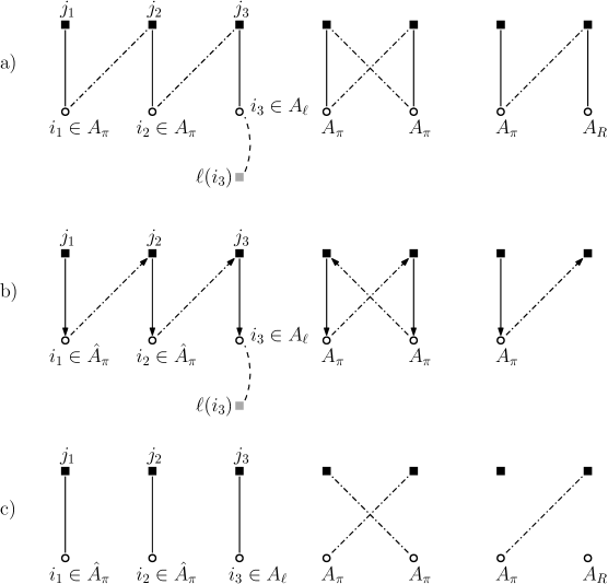
Figure 1: White circles represent the agents, black squares the item set $H$, and grey squares the favorite items. Solid lines represent matching $\tau$, while dashed-dotted lines represent a subset of matching $\pi$. Figure a) shows matching $\tau$, matching $\pi$ for the agents in $A_{\pi}$, and the $\ell(i)$ items for the agents in $A_{\ell}$. Figure b) shows graph $D$ (and the $\ell(i)$’s). Figure c) shows matching $\rho$.

Let $\hat{A}_{\pi}\subseteq A_{\pi}$ be the set of nodes that can reach $A_{\ell}$ in the digraph $D$. By construction, each $i\in A_{\pi}$ is either contained in a cycle inside $A_{\pi}\cup H$, or on a directed path ending in $A_{\ell}\cup H$; these paths start in $H$ and may terminate in either $H$ or $A_{\ell}$. We choose $\hat{A}_{\pi}$ as the set of nodes where the path terminates in $A_{\ell}$.

We define the matching $\rho:\,A\to H\cup\{\bot\}$ as

$$\rho(i):=\begin{cases}\bot\,,&\mbox{if }i\in A_{R}\,,\\ \tau(i)\,,&\mbox{if }i\in A_{\ell}\cup\hat{A}_{\pi}\,,\\ \pi(i)\,,&\mbox{if }i\in A_{\pi}\setminus\hat{A}_{\pi}\,.\\ \end{cases}$$

Claim.

$\rho$ is a matching.

Proof.

For a contradiction, assume $j=\pi(i^{\prime})=\tau(i)$ for $i^{\prime}\in A_{\pi}\setminus\hat{A}_{\pi}$ and $i\in A_{\ell}\cup\hat{A}_{\pi}$. Then, $(i^{\prime},j),(j,i)$ forms 2-hop directed path from $i^{\prime}$ to $i$ in $D$. Since $i\in\hat{A}_{\pi}$, there is a directed path $P$ from $i$ to a node in $A_{\ell}$. Concatenating these two paths gives a directed path from $i^{\prime}$ to a node in $A_{\ell}$. Thus, $i^{\prime}\in\hat{A}_{\pi}$, a contradiction. ∎

It remains to show

$$\prod_{i\in A_{\ell}\cup\hat{A}_{\pi}}v_{i}(\tau(i))^{w_{i}}\geq\prod_{i\in A_{\ell}}v_{i}(\ell(i))^{w_{i}}\prod_{i\in\overline{A}_{\pi}}v_{i}(\pi(i))^{w_{i}}\,.$$ (2)

The set of nodes in $A_{\ell}\cup\hat{A}_{\pi}$ are covered by maximal directed paths in $D$ terminating in $A_{\ell}$. First, consider a length one path $P=(j,i)$ that comprises an item node $j\in H$ and an agent node $i\in A_{\pi}$ such that $j=\tau(i)$, and $j$ has no incoming arcs in $D$. Then, $v_{i}(\tau(i))\geq v_{i}(\ell(i))$ by Claim 3.14.

Consider now a longer path $P=(j_{1},i_{1},j_{2},i_{2},\ldots,j_{k},i_{k})$ for $k>1$, where $j_{t}\in H$ are item nodes, $i_{t}\in\hat{A}_{\pi}$ for $t<k$ and $i_{k}\in A_{\ell}$. Thus, $\tau(i_{t})=j_{t}$ for $t\in[k]$ and $\pi(i_{t})=j_{t+1}$ for $t\in[k-1]$. We claim that

$$\prod_{t=1}^{k}v_{i_{t}}(\tau(i_{t}))^{w_{i_{t}}}\geq v_{i_{k}}(\ell(i_{k}))^{w_{i_{k}}}\prod_{t=1}^{k-1}v_{i_{t}}(\pi(i_{t}))^{w_{i_{t}}}\,.$$

The proof follows the same lines as the proof of Claim 3.14. Indeed, if this equality does not hold, then there would exist a better matching $\overline{\tau}:\,A\to G$ defined as $\overline{\tau}(i_{k}):=\ell(i_{k})$, and $\overline{\tau}(i_{t}):=j_{t+1}=\pi(i_{t})$ for $t=1,2,\ldots,k-1$, and $\overline{\tau}(h):=\tau(h)$ for $h\neq i$.

The inequality (2) follows by multiplying these inequalities over all maximal directed paths in $D$ that terminate in $A_{\ell}$. This completes the proof. ∎

4 Finding fair and efficient allocations

4.1 Completing the partial allocation

In this section, we derive Theorem 1.2 from Lemma 2.1. The proof of Lemma 2.1, describing the subroutine MakeFairOrEfficient is given in Section 4.2. The algorithm described in Theorem 1.2 is Algorithm 3. It uses two subroutines: MakeFairOrEfficient, and the envy-free cycle procedure EnvyFreeCycle from [39], described below.

Input: Allocation $\mathcal{S}$ that is $\alpha$-approximation to the NSW problem $(A,G,(v_{i})_{i\in A})$.

Output: Allocation $\mathcal{T}$ that is $\nicefrac{{1}}{{2}}$-EFX and $2\alpha$-approximation to the symmetric NSW problem.

1 $\mathcal{T}\leftarrow\mathcal{S}$

2 repeat

       $\mathcal{T}\leftarrow\textnormal{{MakeFairOrEfficient}}(\mathcal{T})$

        // Algorithm 4

3      

4until $\mathcal{T}$ is not $\nicefrac{{1}}{{2}}$-EFX

$U\leftarrow G\setminus\cup_{i}T_{i}$

  // set of unallocated items

5 repeat

6       Let $j\in U$ be such that $v_{i}(T_{i})<v_{i}(j)$ for some agent $i$

7       $T_{i}\leftarrow\{j\}$

8       $U\leftarrow(U\cup T_{i})-j$

9      

10until $v_{i}(T_{i})\geq v_{i}(j),\forall i\in A,\forall j\in U$

11$\mathcal{T}\leftarrow$ EnvyFreeCycle($\mathcal{T},U$)

12 return $\mathcal{T}$

Algorithm 3 Guaranteeing $\nicefrac{{1}}{{2}}$-EFX for the symmetric NSW problem

The input of Algorithm 3 is an allocation $\mathcal{S}$ that is $\alpha$-approximation to the symmetric NSW problem. It then repeatedly calls MakeFairOrEfficient($\mathcal{T}$) (Algorithm 4) until the final allocation is $\nicefrac{{1}}{{2}}$-EFX and $2\alpha$-approximation to the symmetric NSW problem. Recall that the output of this subroutine is either a partial allocation $\mathcal{T}^{\prime}$ that satisfies either $\operatorname*{NSW}(\mathcal{T}^{\prime})\geq\operatorname*{NSW}(\mathcal{T})$ and $\cup_{i}T_{i}^{\prime}\subsetneq\cup_{i}T_{i}$, or $\operatorname*{NSW}(\mathcal{T}^{\prime})\geq\nicefrac{{1}}{{2}}\operatorname*{NSW}(\mathcal{T})$ and $\mathcal{T}^{\prime}$ is $\nicefrac{{1}}{{2}}$-EFX. Since $\cup_{i}T_{i}^{\prime}\subsetneq\cup_{i}T_{i}$ in each call in the first case, the number of calls to Algorithm 4 is at most $m$.

At this point, we have an $\nicefrac{{1}}{{2}}$-EFX partial allocation $\mathcal{T}$ with $\operatorname*{NSW}(\mathcal{T})\geq\tfrac{1}{2}\operatorname*{NSW}(\mathcal{S})$. The rest of Algorithm 3 allocates the remaining items $U=G\setminus\cup_{i\in A}T_{i}$ so that $\operatorname*{NSW}(\mathcal{T})$ does not decrease, and the $\nicefrac{{1}}{{2}}$-EFX property is maintained.

First, we modify the allocation in the second repeat loop to ensure that each agent’s value for their bundle is at least their value for each remaining item in $U$. This is done by swapping an agent’s bundle $T_{i}$ with a singleton item $j\in U$ whenever $i$ values $j$ more than the entire bundle $T_{i}$.

Finally, we run the envy-cycle procedure EnvyFreeCycle($\mathcal{T},U$) from [39] to allocate the remaining items in $U$, starting with the allocation $\mathcal{T}$. The envy-cycle procedure maintains the directed (envy) graph $D=(A,E)$, where $(i,j)\in E$ if $i$ envies $j$’s bundle, i.e., $v_{i}(Y_{i})<v_{i}(Y_{j})$. If there is a cycle in $G$, then we can circulate bundles along the cycle to improve each agent’s utility. Otherwise, there must be a source agent in $G$, whom no agent envies. We then assign an arbitrary item from $U$ to a source agent. We update the envy graph, and iterate until $U$ is fully assigned.

We now verify the correctness and efficiency of this algorithm.

Lemma 4.1.

The second repeat loop of Algorithm 3 is repeated at most $nm$ times. It maintains the $\nicefrac{{1}}{{2}}$-EFX and $\operatorname*{NSW}(\mathcal{T})$ is non-decreasing.

Proof.

The bound on the number of swaps follows since every agent $i\in A$ may swap their bundle at most $m$ times. After the first swap, they maintain a singleton bundle, and they can swap their bundle for the same item $j$ only once, since their valuation $v_{i}(T_{i})$ strictly increases in each swap.

It is immediate that $\operatorname*{NSW}(\mathcal{T})$ is non-decreasing. It is left to show that the $\nicefrac{{1}}{{2}}$-EFX property is maintained. Let $i\in A$ be the agent who swapped their bundle $T_{i}$ for $T^{\prime}_{i}=\{j\}$ in the current iteration. Then, the value of $i$’s own bundle increased while the allocation of everyone else remained the same. Hence, agent $i$ cannot violate the $\nicefrac{{1}}{{2}}$-EFX property. For the other agents $k\neq i$, $v_{k}(T_{k})\geq\nicefrac{{1}}{{2}}\cdot v_{k}(T_{i}^{\prime}-g)$ for all $g\in T_{i}^{\prime}$ trivially holds, since $T_{i}^{\prime}$ is a singleton. ∎

The property (3) below is satisfied after the second repeat loop. Hence, the next lemma completes the analysis of Algorithm 3.

Lemma 4.2.

The subroutine EnvyFreeCycle($\mathcal{T},U$) terminates in $O(n^{3}m)$ time, and $\operatorname*{NSW}(\mathcal{T})$ is non-decreasing. Assume that $\mathcal{T}=(T_{i})_{i\in A}$ is $\nicefrac{{1}}{{2}}$-EFX, and

$$v_{i}(T_{i})\geq v_{i}(j)\quad\forall i\in A,\forall j\in U\,.$$ (3)

Then, EnvyFreeCycle($\mathcal{T},U$) also maintains the $\nicefrac{{1}}{{2}}$-EFX property.

Proof.

The running time analysis is the same as in [39]. Finding and removing a cycle in the envy-graph can be done in $O(n^{2})$ time. Further, whenever swapping around a cycle, at least one edge is removed from the envy graph. New edges can only be added when we allocate new items from $U$, with at most $n$ edges every time. Since $|U|\leq m$, the total number of new edges added throughout is $nm$. This yields the overall $O(n^{3}m)$ bound.

Again, it is immediate that $\operatorname*{NSW}(\mathcal{T})$ is non-decreasing in every step. We need to show that the $\nicefrac{{1}}{{2}}$-EFX property is maintained both when swapping around cycles and when adding new items from $U$. When swapping around a cycle, this follows since the set of bundles remains the same, and no agent’s value decreases.

Consider the case when a source agent say $i$, gets a new item $j$: their new bundle becomes $T^{\prime}_{i}=T_{i}+j$. Note that $i$ is the only agent whose value increases; all other bundles remain the same. We need to show that for any $k\neq i$,

$$v_{k}(T_{k})\geq\tfrac{1}{2}v_{k}(T^{\prime}_{i}-g)\quad\forall g\in T^{\prime}_{i}\,.$$

We show that

$$v_{k}(T^{\prime}_{i}-g)=v_{k}(T_{i}+j-g)\leq v_{k}(T_{i})+v_{k}(j)\leq 2v_{k}(T_{k})\,.$$

Here, the first inequality follows by subadditivity and monotonicity. The second inequality uses (3), and that $v_{k}(T_{k})\geq v_{k}(T_{i})$, since $i$ was a source node in the envy graph. ∎

4.2 Finding a fair or an efficient allocation

In this Section, we prove Lemma 2.1. The subroutine MakeFairOrEfficient($\mathcal{T}$) is shown in Algorithm 4, and generalizes an algorithm by Caragiannis, Gravin, and Huang [13] from additive to subadditive valuations. We begin with defining the notions of $\nicefrac{{1}}{{2}}$-EFX feasible bundles and graph.

Definition 4.3 ($\nicefrac{{1}}{{2}}$-EFX feasible bundles and graph).

Given a partial allocation $\mathcal{T}=(T_{i})_{i\in A}$, we say that $T_{k}$ is a $\nicefrac{{1}}{{2}}$-EFX feasible bundle for agent $i$, if

$$v_{i}(T_{k})\geq\tfrac{1}{2}\max_{\ell\in A,j\in T_{\ell}}v_{i}(T_{\ell}-j)\,.$$

The $\nicefrac{{1}}{{2}}$-EFX feasibility graph of $\mathcal{T}$ is a bipartite graph $\mathcal{K}=(A\cup\mathcal{T},E)$ where the edge set $E$ is defined as:

$$E= \left\{(i,T_{i})\ |\ T_{i}\text{ is }\text{$\nicefrac{{1}}{{2}}$-EFX feasible for }i\right\}\ \ \cup$$ (4)

$$\left\{(i,T_{k})\ |\ v_{i}(T_{k})>2v_{i}(T_{i})\text{ and }v_{i}(T_{k})\geq\max_{\ell\in A,j\in T_{\ell}}v_{i}(T_{\ell}-j)\right\}\,.$$

The following claim can be easily verified using the definition.

Claim 4.4.

The degree of every node $i\in A$ is at least 1 in the graph $\mathcal{K}=(A\cup\mathcal{T},E)$.

In this section, a matching will refer to a matching between agents and bundles (and not between agents and items as in previous sections). Thus, a matching is a mapping $\rho:A\to\mathcal{T}\cup\{\bot\}$ such that $\rho(i)=\rho(k)$ implies $\rho(i)=\rho(k)=\bot$. A perfect matching has $\rho(i)\neq\bot$ for every $i\in A$. Matchings may use pairs $(i,T_{k})$ that are not in $E$; we say that $\rho$ is a matching in the bipartite graph $\mathcal{K}=(A\cup\mathcal{T},E)$ if $(i,\rho(i))\in E$ whenever $\rho(i)\neq\{\bot\}$. For two matchings $\rho$ and $\tau$, an alternating path between $\rho$ and $\tau$ is a path $P=(i_{1},S_{i_{1}},i_{2},\ldots,S_{i_{k-1}},i_{\ell},S_{i_{\ell}})$ such that $\rho(i_{t})=S_{i_{t}}$, $t=1,\ldots,\ell$, $\tau(i_{t+1})=S_{i_{t}}$, $t=1,\ldots,\ell-1$. The following lemma is immediate from the definition of the $\nicefrac{{1}}{{2}}$-EFX feasibility graph.

Lemma 4.5.

If the $\nicefrac{{1}}{{2}}$-EFX feasibility graph $\mathcal{K}=(A\cup\mathcal{T},E)$ of an allocation $\mathcal{T}$ contains a perfect matching $\rho$, then $(i,\rho(i))_{i\in A}$ is a $\nicefrac{{1}}{{2}}$-EFX allocation.

Input: Partial allocation $\mathcal{T}$.

Output: Partial allocation $\mathcal{R}$ such that either $\operatorname*{NSW}(\mathcal{R})\geq\operatorname*{NSW}(\mathcal{T})$ and $\cup_{i}R_{i}\subsetneq\cup_{i}T_{i}$, or $\operatorname*{NSW}(\mathcal{R})\geq\tfrac{1}{2}\operatorname*{NSW}(\mathcal{T})$ and $\mathcal{R}$ is $\nicefrac{{1}}{{2}}$-EFX.

1 $\mathcal{S}\leftarrow\mathcal{T}$

2 repeat

       $\mathcal{K}=(A\cup\mathcal{S},E)\leftarrow\nicefrac{{1}}{{2}}$-EFX feasibility graph of $\mathcal{S}$

        // Definition 4.3

       $\mathcal{L}\leftarrow\{S_{i},i\in A\ |\ S_{i}\subsetneq T_{i}\}$

        // set of trimmed down bundles

       Define matching $\tau$ with $\tau(i)=S_{i}$ for all $i\in A$

        // candidate matching

       $\rho\leftarrow$ matching in $\mathcal{K}$ where

        // Lemma 4.6

3      

• all bundles in $\mathcal{L}$ are matched,

• $|\{i:\rho(i)=S_{i}\}|$ is maximized subject to $(a)$, and

• $\rho$ is maximum subject to $(a)$ and $(b)$

4      if $\exists i_{1}\in A$ not matched in $\rho$ then

5             $(S_{h},g_{h})\leftarrow\arg\max_{k\in A,g\in S_{k}}v_{i_{1}}(S_{k}-g)$

6             if $v_{h}(S_{h}-g_{h})\geq\frac{1}{2}\cdot v_{h}(T_{h})$ then

7                  $S_{h}\leftarrow S_{h}-g_{h}$

8            else

                   $P=(i_{1},S_{i_{1}},i_{2},\dots,S_{i_{\ell-1}},i_{\ell},S_{i_{\ell}})$ $\leftarrow$ alternating path between $\tau$ and $\rho$ starting at $i_{1}$ and ending at either $S_{i_{\ell}}=S_{h}$ or an unmatched $S_{i_{\ell}}\neq S_{h}$

                    // Lemma 4.7

9                   Construct $\mathcal{R}$:

10                      $R_{i_{1}}\leftarrow S_{h}-g_{h}$

11                      for $f\leftarrow 2$ to $\ell$ do $R_{i_{f}}\leftarrow S_{i_{f-1}}$

12                      for $i\in A\setminus(\{i_{1},\dots,i_{\ell}\}\cup\{h\})$ do $R_{i}\leftarrow T_{i}$

13                   if $P$ ends at an unmatched bundle $S_{i_{\ell}}\neq S_{h}$ then

14                            $R_{h}\leftarrow T_{h}\setminus(S_{h}-g_{h})$

15                        

16                  return $\mathcal{R}$

17                  

18            

19      

20until $\rho$ is a perfect matching in $\mathcal{K}$

21return $\mathcal{R}=(\rho(i))_{i\in A}$

Algorithm 4 MakeFairOrEfficient($\mathcal{T}$)

We now give an overview of Algorithm 4. For an input partial allocation $\mathcal{T}=(T_{i})_{i\in A}$, it returns a partial allocation $\mathcal{R}$ that satisfies one of the alternatives in Lemma 2.1: either (i) $\operatorname*{NSW}(\mathcal{R})\geq\operatorname*{NSW}(\mathcal{T})$ and $\cup_{i}R_{i}\subsetneq\cup_{i}T_{i}$, or (ii) $\operatorname*{NSW}(\mathcal{R})\geq\tfrac{1}{2}\operatorname*{NSW}(\mathcal{T})$ and $\mathcal{R}$ is $\nicefrac{{1}}{{2}}$-EFX.

The algorithm gradually ‘trims down’ the bundles $\mathcal{T}$. That is, we maintain a partial allocation $\mathcal{S}=(S_{i})_{i\in A}$ with $S_{i}\subseteq T_{i}$ throughout. Every main loop of the algorithm either terminates by constructing an allocation $\mathcal{R}$ satisfying (ii), or removes an item from one of the $S_{h}$ sets. The other possible termination option is when the $\nicefrac{{1}}{{2}}$-EFX feasibility graph of $\mathcal{S}$ contains a perfect matching $\rho$. In this case, we return $\mathcal{R}=(\rho(i))_{i\in A}$. This is a $\nicefrac{{1}}{{2}}$-EFX allocation by Lemma 4.5; Lemma 4.8 shows it also satisfies $\operatorname*{NSW}(\mathcal{R})\geq\tfrac{1}{2}\operatorname*{NSW}(\mathcal{T})$ and is thus a suitable output of type (ii).

At the beginning of each main loop, we define two matchings. The first is the perfect matching $\tau$ that simply defines $\tau(i)=S_{i}$ for all $i\in A$. The second is a matching $\rho$ in $\mathcal{K}$. This is required to satisfy three properties: First, it matches all trimmed down bundles, i.e., all bundles $S_{i}$ with $S_{i}\subsetneq T_{i}$. Second, $|\{i:\rho(i)=S_{i}\}|$ is maximized subject to the first requirement. Third, subject to these requirements, $\rho$ is chosen as a maximal matching. (The existence of such a matching is guaranteed by Lemma 4.6 below).

If $\rho$ is not perfect, then we consider an unmatched agent $i_{1}$, and find the bundle that maximizes $i_{1}$’s utility after removal of one item. Let $(S_{h},g_{h})\in\arg\max_{k\in A,g\in S_{k}}v_{i_{1}}(S_{k}-g)$. If agent $h$’s value of $S_{h}-g_{h}$ is at least $\frac{1}{2}$ times their value for the original bundle $T_{h}$, then we remove $g_{h}$ from $S_{h}$ and the main loop finishes. Otherwise, we construct an alternating path between $\rho$ and $\tau$, denoted as $P=(i_{1},S_{i_{1}},i_{2},S_{i_{2}},\dots,S_{i_{\ell-1}},i_{\ell},S_{i_{\ell}})$, starting with $i_{1}$ and ending with either $S_{i_{\ell}}=S_{h}$ or an unmatched bundle $S_{i_{\ell}}\neq S_{h}$. Lemma 4.7 shows that such a $P$ exists. Using $P$, we construct an allocation $\mathcal{R}$ in line 4. Lemma 4.8 shows that this is a suitable output of type (i).

4.2.1 Analysis

The number of iterations of the repeat loop is at most $m$, because the algorithm remove one item from some bundle in each iteration, in which it does not terminate. Since we can find the maximum matching in line 4 and alternating path in line 4 in strongly polynomial-time, Algorithm 4 runs in strongly polynomial-time.

The next lemma guarantees that the matching $\rho$ is well-defined. The proof follows similarly as in [13].

Lemma 4.6.

In each iteration of the repeat loop in Algorithm 4, a matching exists in $\mathcal{K}$ where all bundles of $\mathcal{L}$ are matched.

Proof.

Let $E^{(t)}$ denote the edge set of the $\nicefrac{{1}}{{2}}$-EFX feasibility graph and $\mathcal{L}^{(t)}$ the set of trimmed down bundles, and $\rho^{(t)}$ the maximum matching in the $t$-th iteration.

We show by induction that there exists a matching $\rho^{(t)}$ such that all bundles in $\mathcal{L}^{(t)}$ are matched. At the beginning of the first iteration, $\mathcal{L}^{(1)}$ is empty, so the claim is clearly true. Suppose the claim is true until the beginning of $(t+1)$-st iteration. Let $\mathcal{S}$ denote the trimmed down bundles in the $t$-th iteration, and let $i_{1}$ be the unmatched agent, and $(S_{h},g_{h})$ the bundle and item selected in line 4.

By the requirement that $|\{i:\rho(i)=S_{i}\}|$ is maximized subject to all trimmed down bundles being matched, we have $(i_{1},S_{i_{1}})\not\in E^{(t)}$. By the choice of $h$, we have $(i,S_{h})\in E^{(t)}$ in the $t$-th iteration.

Note that $\mathcal{L}^{(t+1)}=\mathcal{L}^{(t)}\cup\{h\}$. Consider the $\nicefrac{{1}}{{2}}$-EFX feasibility graph in the $(t+1)$-st iteration. Since all bundles different from $S^{\prime}_{h}:=S_{h}-g_{h}$ remained unchanged, for every edge $(i,S_{k})\in E^{(t)}$ with $k\neq h$ it follows that $(i,S_{k})\in E^{(t+1)}$. According to Definition 4.3, $(i_{1},S_{h}^{\prime})\in E^{(t+1)}$. Let us define $\rho^{\prime}$ as

$$\rho^{\prime}(i):=\begin{cases}S^{\prime}_{h}&\mbox{if }i=i_{1}\,,\\ \rho^{(t)}(i)&\mbox{if }i\neq i_{1}\mbox{ and }\rho^{(t)}(i)\neq S_{h}\,,\\ \bot&\mbox{otherwise}\,.\end{cases}$$

By the above, this gives a matching in $E^{(t+1)}$, and it matches all bundles in $\mathcal{L}^{(t+1)}=\mathcal{L}^{(t)}\cup\{h\}$. ∎

Lemma 4.7.

The alternating path $P$, as described in line 4 of Algorithm 4, exists.

Proof.

Since $i_{1}$ is an unmatched agent and the requirement that $|\{i:\rho(i)=S_{i}\}|$ is maximized subject to all trimmed down bundles being matched in the maximum matching $\rho$ in line 4, we must have $(i_{1},S_{i_{1}})\not\in E$. If $\rho(i_{2})=S_{i_{1}}$ for an agent $i_{2}\in A$, then we continue with $S_{i_{2}}$, otherwise we stop. Continuing this way, we eventually reach either $S_{i_{\ell}}=S_{h}$ or an unmatched bundle $S_{i_{\ell}}\neq S_{h}$. ∎

Lemma 4.8.

If Algorithm 4 returns an allocation $\mathcal{R}$ in line 4, then $\operatorname*{NSW}(\mathcal{R})\geq\tfrac{1}{2}\operatorname*{NSW}(\mathcal{T})$ and $\mathcal{R}$ is $\nicefrac{{1}}{{2}}$-EFX. If it returns $\mathcal{R}$ in line 4, then $\operatorname*{NSW}(\mathcal{R})\geq\operatorname*{NSW}(\mathcal{T})$ and $\cup_{i}R_{i}\subsetneq\cup_{i}T_{i}$.

Proof.

Let us start with the case when a perfect matching $\mathcal{R}=(\rho(i))_{i\in A}$ is returned in line 4. The $\nicefrac{{1}}{{2}}$-EFX property follows by Lemma 4.5. Let us show $\operatorname*{NSW}(\mathcal{R})\geq\tfrac{1}{2}\operatorname*{NSW}(\mathcal{T})$.

Throughout the algorithm, $v_{i}(S_{i})\geq\frac{1}{2}v_{i}(T_{i})$ is maintained according to the condition on bundle trimming. By Claim 4.4, either $R_{i}=S_{i}$, or $v_{i}(R_{i})>2v_{i}(S_{i})$. Therefore, we have

$$\forall i :v_{i}(R_{i})\geq v_{i}(S_{i})\geq\frac{1}{2}v_{i}(T_{i})\,.$$ (5)

Consequently,

$$\operatorname*{NSW}(\mathcal{R})=\prod_{i\in A}\left(v_{i}(R_{i})\right)^{1/n}\geq\frac{1}{2}\cdot\prod_{i\in A}\left(v_{i}(T_{i})\right)^{1/n}\geq\tfrac{1}{2}\operatorname*{NSW}(\mathcal{T})\,.$$

Consider now the case when the algorithm terminated with $\mathcal{R}$ in line 4. We need to show $\operatorname*{NSW}(\mathcal{R})\geq\operatorname*{NSW}(\mathcal{T})$ and $\cup_{i}R_{i}\subsetneq\cup_{i}T_{i}$. Two cases here depend on whether $S_{i_{\ell}}=S_{h}$ or $S_{i_{\ell}}(\neq S_{h})$ is an unmatched bundle. For the first case, we have

$$v_{i_{f}}(R_{i_{f}}) =v_{i_{f}}(S_{i_{f-1}})>2v_{i_{f}}(S_{i_{f}})\geq v_{i_{f}}(T_{i_{f}}),\ \forall f\in\{2,\dots,\ell\}\,,$$

$$v_{i_{1}}(R_{i_{1}}) =v_{i_{1}}(S_{h}-g_{h})>2v_{i_{1}}(S_{i_{1}})\geq v_{i_{1}}(T_{i_{1}})$$

This implies

$$\operatorname*{NSW}(\mathcal{R})=\prod_{i\in A}\big{(}v_{i}(R_{i})\big{)}^{1/n}>\prod_{i\in A}\big{(}v_{i}(T_{i})\big{)}^{1/n}=\operatorname*{NSW}(\mathcal{T})\,.$$

Since we do not assign $g_{h}$ to any agent in $\mathcal{R}$, we must have $\cup_{i}R_{i}\subsetneq\cup_{i}T_{i}$.

For the second case, since $S_{i_{\ell}}$ is an unmatched bundle in $\rho$ by the choice of the path $P$, we have $S_{i_{\ell}}\notin\mathcal{L}$ by the requirements on $\rho$. That is, $S_{i_{\ell}}=T_{i_{\ell}}$. By Claim 4.4, we have

$$v_{i_{\ell}}(R_{i_{\ell}}) =v_{i_{\ell}}(S_{i_{\ell-1}})>2v_{i_{\ell}}(S_{i_{\ell}})=2v_{i_{\ell}}(T_{i_{\ell}})\,,$$ (6)

$$v_{i_{f}}(R_{i_{f}}) =v_{i_{f}}(S_{i_{f-1}})>2v_{i_{f}}(S_{i_{f}})\geq v_{i_{f}}(T_{i_{f}}),\ \forall f\in\{2,\dots,\ell-1\}\,,$$

$$v_{i_{1}}(R_{i_{1}}) =v_{i_{1}}(S_{h}-g_{h})>2v_{i_{1}}(S_{i_{1}})\geq v_{i_{1}}(T_{i_{1}})$$

$$v_{h}(R_{h}) =v_{h}(X_{h}\setminus(S_{h}-g_{h}))>\tfrac{1}{2}v_{h}(T_{h})\,.$$

The last inequality follows from subadditivity using $v_{h}(T_{h})\leq v_{h}(S_{h}-g_{h})+v_{h}(T_{h}\setminus(S_{h}-g_{h}))$. Using (6), we get

$$\operatorname*{NSW}(\mathcal{R})=\prod_{i\in A}\big{(}v_{i}(R_{i})\big{)}^{1/n}>\prod_{i\in A}\big{(}v_{i}(T_{i})\big{)}^{1/n}=\operatorname*{NSW}(\mathcal{T})\,.$$

Finally, since we do not assign items in $T_{i_{l}}$ to any agent in $\mathcal{R}$, we must have $\cup_{i}R_{i}\subsetneq\cup_{i}T_{i}$. Note that if $T_{i_{l}}=\emptyset$, then $\operatorname*{NSW}(\mathcal{T})=0$ and $R_{i}=\emptyset,\forall i$ is a suitable output of type (ii). ∎

5 Conclusion

We have shown a $(4+\varepsilon)$-approximation algorithm for the symmetric NSW problem with submodular valuations, which is the largest natural class of valuations that allows a constant-factor approximation (using value queries) even for utilitarian social welfare. Moreover, our algorithm gives an $\mathrm{e}(2+nw_{\max}+\varepsilon)$-approximation algorithm for the asymmetric NSW problem under submodular valuations. However, there are still several directions and open problems to explore. An obvious one is to improve the approximation ratio for the symmetric case. The current hardness of approximation stands at $\frac{\mathrm{e}}{\mathrm{e}-1}\simeq 1.58$ for submodular valuations, which is the same as the optimal factor for maximizing utilitarian social welfare. It would be interesting to prove a separation between the two optimization objectives for submodular valuations.

Another open problem is the asymmetric NSW problem. The goal is to get a constant-factor approximation independent of the weights $w_{i}$. For the asymmetric problem, getting a universal constant factor is open even in the basic case of additive valuations. The simplest case not covered by our algorithm is when one agent has weight $1/2$ and all other agents have weight $1/2n$.

There are several open questions on the existence of EFX and its relaxations for submodular valuations. We mention two: First, does there exist a (complete) $\alpha$-EFX allocations for $\alpha>1/2$? Here, we do not make any efficiency requirements. Second, does there exist an EF1 allocation with high NSW value? Note that [14] shows that for additive valuations, the optimal NSW allocation is EF1.

Appendix A Appendix

We now give a slight strengthening of Theorem 1.1 for the asymmetric case. For $\nu\geq 0$, let us define

$$\phi(\nu)\coloneqq\sup_{x\in(0,1]}2^{1-x}\left(1+\frac{\nu}{x}\right)^{x}\,.$$

This quantity will be used in our approximation guarantee.

Theorem A.1.

For any $\varepsilon>0$, there is a deterministic polynomial-time $(\phi(nw_{\max})+\varepsilon)\mathrm{e}$-approximation algorithm for the asymmetric Nash social welfare problem with submodular valuations. The number of arithmetic operations and oracle calls is polynomial in $n$, $m$, and $1/\varepsilon$.

We can upper bound the function $\phi(\nu)$ as follows. In particular, the bound becomes $(nw_{\max}+1+\varepsilon)\mathrm{e}$ for $w_{\max}\geq 3.5/n$.

Lemma A.2.

For $\nu\geq 0$, $\phi(\nu)\leq\nu+2$. For $\nu\geq 3.5$, $\phi(\nu)=\nu+1$.

Proof.

The first part follows by the AM-GM inequality: for each $x\in(0,1]$, $2^{1-x}(1+\frac{\nu}{x})^{x}\leq(1-x)2+x(1+\frac{\nu}{x})=\nu+2-x$. For the second part, let us take the derivative of $\ln\phi(x)=(1-x)\ln 2+x\ln(1+\frac{\nu}{x})$:

$$(\ln\phi)^{\prime}(x) = -(\ln 2)+\ln(1+\frac{\nu}{x})+\frac{x}{1+\nu/x}(-\frac{\nu}{x^{2}})$$

$$= -(\ln 2)+\ln(1+\frac{\nu}{x})-\frac{\nu}{x+\nu}.$$

This derivative is decreasing in $x$, and evaluated at $1$ gives $-(\ln 2)+\ln(1+\nu)-\frac{\nu}{1+\nu}$. This function is increasing in $\nu$ and positive for $\nu\geq 3.5$ (in fact for $\nu\geq 3.32$). Therefore, $(\ln\phi)^{\prime}(x)$ is positive for $\nu\geq 3.5$ and $x\in(0,1]$, which means that $\phi(x)$ attains its maximum over $(0,1]$ at $x=1$. ∎

The proof of Theorem A.1 follows the same way as the proof of Theorem 1.1, with the only difference that Lemma 3.8 is replaced by the following stronger version.

Lemma A.3.

Let $\bar{\varepsilon}\geq 0$, and let $\mathcal{R}=(R_{i})_{i\in\bar{A}}$ be an $\bar{\varepsilon}$-local optimum with respect to the endowed valuations $\bar{v}_{i}$ that are submodular. Let $(S_{1},S_{2},\ldots,S_{n})$ denote any partition of the set $J$, and let $h_{i}\geq 0$ such that $\sum_{i\in A}h_{i}\leq n$. Then,

$$\prod_{i\in A\setminus\bar{A}}h_{i}^{w_{i}}\prod_{i\in\bar{A}}\left(\frac{v_{i}(S_{i})}{\max\{v_{i}(\ell(i)),v_{i}(R_{i})\}}+h_{i}\right)^{w_{i}}\leq(1+\varepsilon)\phi(nw_{\max})\mathrm{e}\,.$$

Before proving Lemma A.3, let us give a bound on the value of any set relative to our local optimum.

Proposition A.4.

Let $\mathcal{R}=(R_{i})_{i\in A}$ be a $\bar{\varepsilon}$-local optimum and $S\subseteq J$ any set of items. Then

$$\frac{v_{i}(S)}{\max\{v_{i}(R_{i}),v_{i}(\ell(i)\}}\leq-1+2(1+\bar{\varepsilon})^{|S|/w_{i}}\mathrm{e}^{\sum_{j\in S}p_{j}/w_{i}}.$$

Proof.

By Lemma 3.5,

$$\frac{v_{i}(\ell(i))+v_{i}(S)}{v_{i}(\ell(i))+v_{i}(R_{i})}=\frac{\bar{v}_{i}(S)}{\bar{v}_{i}(R_{i})}\leq\frac{\bar{v}_{i}(R_{i}\cup S)}{\bar{v}_{i}(R_{i})}\leq(1+\bar{\varepsilon})^{|S|/w_{i}}\mathrm{e}^{\sum_{j\in S}p_{j}/w_{i}}.$$

Let $\lambda=\frac{v_{i}(R_{i})}{v_{i}(\ell(i))}$. We can rewrite the inequality above as follows:

$$\frac{1+\frac{v_{i}(S)}{v_{i}(\ell_{i})}}{1+\lambda}\leq(1+\bar{\varepsilon})^{|S|/w_{i}}\mathrm{e}^{\sum_{j\in S}p_{j}/w_{i}}.$$

From here,

$$\frac{v_{i}(S)}{v_{i}(\ell_{i})}\leq(1+\lambda)(1+\bar{\varepsilon})^{|S|/w_{i}}\mathrm{e}^{\sum_{j\in S}p_{j}/w_{i}}-1.$$

We use this inequality if $0\leq\lambda\leq 1$. If $\lambda>1$, we divide by $\lambda$ to obtain:

$$\frac{v_{i}(S)}{v_{i}(R_{i})}\leq(1/\lambda+1)(1+\bar{\varepsilon})^{|S|/w_{i}}\mathrm{e}^{\sum_{j\in S}p_{j}/w_{i}}-1/\lambda.$$

Either way, the worst case is $\lambda=1$, which gives

$$\frac{v_{i}(S)}{\max\{v_{i}(\ell(i)),v_{i}(R_{i})\}}\leq 2(1+\bar{\varepsilon})^{|S|/w_{i}}\mathrm{e}^{\sum_{j\in S}p_{j}/w_{i}}-1.\qed$$

Proof of Lemma A.3.

By Proposition A.4,

$$\frac{v_{i}(S_{i})}{\max\{v_{i}(R_{i}),v_{i}(\ell(i)\}}\leq 2(1+\bar{\varepsilon})^{|S_{i}|/w_{i}}\mathrm{e}^{\sum_{j\in S_{i}}p_{j}/w_{i}}-1.$$

Our goal is to bound the left-hand side of Lemma A.3, which is a product of $\frac{v_{i}(S_{i})}{\max\{v_{i}(R_{i}),v_{i}(\ell(i)\}}+h_{i}$ for some $h_{i}\geq 0$, $\sum h_{i}\leq n$. Let us divide the agents in $\bar{A}$ into two groups, $A_{1}=\{i\in\bar{A}:h_{i}\leq 1\}$ and $A_{2}=\{i\in\bar{A}:h_{i}\geq 2\}$.

First, let us bound

$$\prod_{i\in A_{1}}\left(\frac{v_{i}(S_{i})}{\max\{v_{i}(R_{i}),v_{i}(\ell(i)\}}+h_{i}\right)^{w_{i}} \leq \prod_{i\in A_{1}}\left(2(1+\bar{\varepsilon})^{|S_{i}|/w_{i}}\mathrm{e}^{\sum_{j\in S_{i}}p_{j}/w_{i}}-1+h_{i}\right)^{w_{i}}$$

$$\leq \prod_{i\in A_{1}}\left(2(1+\bar{\varepsilon})^{|S_{i}|/w_{i}}\mathrm{e}^{\sum_{j\in S_{i}}p_{j}/w_{i}}\right)^{w_{i}}$$

$$\leq 2^{w(A_{1})}(1+\bar{\varepsilon})^{\sum_{i\in A_{1}}|S_{i}|}\mathrm{e}^{\sum_{i\in A_{1}}p(S_{i})}$$

using Proposition A.4 and the fact that $h_{i}\leq 1$ for $i\in A_{1}$.

Next, we consider the agents $i\in A_{2}$, i.e. those where $h_{i}\geq 2$:

$$\prod_{i\in A_{2}}\left(\frac{v_{i}(S_{i})}{\max\{v_{i}(R_{i}),v_{i}(\ell(i)\}}+h_{i}\right)^{w_{i}} \leq \prod_{i\in A_{2}}\left(2(1+\bar{\varepsilon})^{|S_{i}|/w_{i}}\mathrm{e}^{\sum_{j\in S_{i}}p_{j}/w_{i}}-1+h_{i}\right)^{w_{i}}$$

$$\leq \prod_{i\in A_{2}}\left((1+\bar{\varepsilon})^{|S_{i}|/w_{i}}\ \mathrm{e}^{\sum_{j\in S_{i}}p_{j}/w_{i}}(2-1+h_{i})\right)^{w_{i}}$$

$$\leq (1+\bar{\varepsilon})^{\sum_{i\in A_{2}}|S_{i}|}\mathrm{e}^{\sum_{i\in A_{2}}p(S_{i})}\prod_{i\in A_{2}}(1+h_{i})^{w_{i}}.$$

Finally, the left-hand side of Lemma A.3 contains

$$\prod_{i\in A\setminus\bar{A}}h_{i}^{w_{i}}\leq\prod_{i\in A\setminus\bar{A}}(1+h_{i})^{w_{i}}.$$

We estimate the product of factors involving $(1+h_{i})$ using the AM-GM inequality: Let $A^{\prime}=(A\setminus\bar{A})\cup A_{2}$, and $\omega=\sum_{i\in A^{\prime}}w_{i}$. We can assume that $\omega>0$; for $\omega=0$ we obtain a bound which is equal to the limit as $\omega\to 0$. Hence:

$$\prod_{i\in A^{\prime}}(1+h_{i})^{w_{i}/\omega}\leq\frac{1}{\omega}\sum_{i\in A^{\prime}}w_{i}(1+h_{i})\leq 1+\frac{w_{\max}}{\omega}\sum_{i\in A^{\prime}}h_{i}\leq 1+\frac{nw_{\max}}{\omega}.$$

So, we obtain $\prod_{i\in A^{\prime}}(1+h_{i})^{w_{i}}\leq\left(1+\frac{nw_{\max}}{\omega}\right)^{\omega}$.

To summarize, we upper-bound the left-hand side of Lemma A.3 by

$$\prod_{i\in A\setminus\bar{A}}(1+h_{i})^{w_{i}}\prod_{i\in A_{1}\cup A_{2}}\left(\frac{v_{i}(S_{i})}{\max\{v_{i}(R_{i}),v_{i}(\ell(i)\}}+h_{i}\right)^{w_{i}}$$

$$\leq \prod_{i\in A^{\prime}}(1+h_{i})^{w_{i}}\cdot 2^{w(A_{1})}(1+\bar{\varepsilon})^{\sum_{i\in A_{1}\cup A_{2}}|S_{i}|}\mathrm{e}^{\sum_{i\in A_{1}\cup A_{2}}p(S_{i})}$$

$$\leq \left(1+\frac{nw_{\max}}{\omega}\right)^{\omega}\cdot 2^{1-\omega}(1+\bar{\varepsilon})^{m}\mathrm{e}$$

$$\leq (1+\varepsilon)\phi(nw_{\max})\mathrm{e}$$

where we used the facts that $w(A_{1})=1-w(A^{\prime})=1-\omega$, the sets $S_{i}$ are disjoint sets of items, and all the prices sum up to at most $1$. The final inequality follows by maximizing over $\omega\in(0,1]$. ∎

References

• [1] G. Amanatidis, G. Birmpas, A. Filos-Ratsikas, A. Hollender, and A. A. Voudouris. Maximum Nash welfare and other stories about EFX. In Proceedings of the Twenty-Ninth International Joint Conference on Artificial Intelligence (IJCAI), pages 24–30, 2020.
• [2] N. Anari, S. O. Gharan, A. Saberi, and M. Singh. Nash social welfare, matrix permanent, and stable polynomials. In Proceedings of the 8th Innovations in Theoretical Computer Science Conference (ITCS), 2017.
• [3] N. Anari, T. Mai, S. O. Gharan, and V. V. Vazirani. Nash social welfare for indivisible items under separable, piecewise-linear concave utilities. In Proceedings of the 29th annual ACM-SIAM Symposium on Discrete Algorithms (SODA), pages 2274–2290. SIAM, 2018.
• [4] N. Bansal and M. Sviridenko. The Santa Claus problem. In Proceedings of the 38th ACM Symposium on Theory of Computing (STOC), pages 31–40, 2006.
• [5] J. B. Barbanel. The geometry of efficient fair division. Cambridge University Press, 2005.
• [6] S. Barman, U. Bhaskar, A. Krishna, and R. G. Sundaram. Tight approximation algorithms for p-mean welfare under subadditive valuations. In 28th Annual European Symposium on Algorithms (ESA), volume 173, pages 11:1–11:17, 2020.
• [7] S. Barman, A. Krishna, P. Kulkarni, and S. Narang. Sublinear approximation algorithm for Nash social welfare with XOS valuations. arXiv preprint arXiv:2110.00767, 2021.
• [8] S. Barman, S. K. Krishnamurthy, and R. Vaish. Finding fair and efficient allocations. In Proceedings of the 2018 ACM Conference on Economics and Computation (EC), pages 557–574, 2018.
• [9] B. Berger, A. Cohen, M. Feldman, and A. Fiat. Almost full EFX exists for four agents. In Proceedings of the 36th Conf. Artif. Intell. (AAAI), 2022.
• [10] S. J. Brams and A. D. Taylor. Fair Division: From cake-cutting to dispute resolution. Cambridge University Press, 1996.
• [11] F. Brandt, V. Conitzer, U. Endriss, J. Lang, and A. D. Procaccia, editors. Handbook of Computational Social Choice. Cambridge University Press, 2016.
• [12] E. Budish. The combinatorial assignment problem: Approximate competitive equilibrium from equal incomes. J. Political Economy, 119(6):1061–1103, 2011.
• [13] I. Caragiannis, N. Gravin, and X. Huang. Envy-freeness up to any item with high Nash welfare: The virtue of donating items. In Proceedings of the 2019 ACM Conference on Economics and Computation (EC), pages 527–545. ACM, 2019.
• [14] I. Caragiannis, D. Kurokawa, H. Moulin, A. D. Procaccia, N. Shah, and J. Wang. The unreasonable fairness of maximum Nash welfare. ACM Transactions on Economics and Computation (TEAC), 7(3):1–32, 2019.
• [15] S. Chae and H. Moulin. Bargaining among groups: an axiomatic viewpoint. International Journal of Game Theory, 39(1-2):71–88, 2010.
• [16] B. R. Chaudhury, Y. K. Cheung, J. Garg, N. Garg, M. Hoefer, and K. Mehlhorn. Fair division of indivisible goods for a class of concave valuations. J. Artif. Intell. Res., 74:111–142, 2022.
• [17] B. R. Chaudhury, J. Garg, and K. Mehlhorn. EFX exists for three agents. In Proceedings of the 21st Conf. Econom. Comput. (EC), pages 1–19. ACM, 2020.
• [18] B. R. Chaudhury, J. Garg, and R. Mehta. Fair and efficient allocations under subadditive valuations. In Proceedings of the AAAI Conference on Artificial Intelligence, pages 5269–5276, 2021.
• [19] B. R. Chaudhury, T. Kavitha, K. Mehlhorn, and A. Sgouritsa. A little charity guarantees almost envy-freeness. SIAM J. Comput., 50(4):1336–1358, 2021.
• [20] R. Cole, N. Devanur, V. Gkatzelis, K. Jain, T. Mai, V. V. Vazirani, and S. Yazdanbod. Convex program duality, Fisher markets, and Nash social welfare. In Proceedings of the 2017 ACM Conference on Economics and Computation (EC), pages 459–460, 2017.
• [21] R. Cole and V. Gkatzelis. Approximating the Nash social welfare with indivisible items. In Proceedings of the 47th ACM Symposium on Theory of Computing (STOC), pages 371–380. ACM, 2015.
• [22] D. M. Degefu, W. He, L. Yuan, and J. H. Zhao. Water allocation in transboundary river basins under water scarcity: a cooperative bargaining approach. Water resources management, 30(12):4451–4466, 2016.
• [23] S. Dobzinski, N. Nisan, and M. Schapira. Approximation algorithms for combinatorial auctions with complement-free bidders. Math. Oper. Res., 35(1):1–13, 2010.
• [24] M. Feldman, S. Mauras, and T. Ponitka. On optimal tradeoffs between EFX and Nash welfare. CoRR, abs/2302.09633, 2023.
• [25] H. Fu, R. Kleinberg, and R. Lavi. Conditional equilibrium outcomes via ascending price processes with applications to combinatorial auctions with item bidding. In Proceedings of the 13th ACM Conference on Electronic Commerce (EC), page 586, 2012.
• [26] J. Garg, M. Hoefer, and K. Mehlhorn. Satiation in Fisher markets and approximation of Nash social welfare. arXiv preprint arXiv:1707.04428, 2017.
• [27] J. Garg, M. Hoefer, and K. Mehlhorn. Approximating the Nash social welfare with budget-additive valuations. In Proceedings of the 29th annual ACM-SIAM Symposium on Discrete Algorithms (SODA), pages 2326–2340. SIAM, 2018.
• [28] J. Garg, E. Husić, and L. A. Végh. Approximating Nash social welfare under rado valuations. In Proceedings of the 53rd Annual ACM SIGACT Symposium on Theory of Computing (STOC), pages 1412–1425, 2021.
• [29] J. Garg, P. Kulkarni, and R. Kulkarni. Approximating Nash social welfare under submodular valuations through (un)matchings. In Proceedings of the ACM-SIAM Symposium on Discrete Algorithms (SODA), pages 2673–2687, 2020.
• [30] H. H, V. der Laan G, and Z. Y. Asymmetric Nash solutions in the river sharing problem. Strategic Behavior and the Environment, 4:321–360, 2014.
• [31] J. C. Harsanyi and R. Selten. A generalized Nash solution for two-person bargaining games with incomplete information. Management science, 18(5-part-2):80–106, 1972.
• [32] E. Kalai. Nonsymmetric Nash solutions and replications of 2-person bargaining. International Journal of Game Theory, 6(3):129–133, 1977.
• [33] M. Kaneko and K. Nakamura. The Nash social welfare function. Econometrica: Journal of the Econometric Society, pages 423–435, 1979.
• [34] F. Kelly. Charging and rate control for elastic traffic. European transactions on Telecommunications, 8(1):33–37, 1997.
• [35] A. Laruelle and F. Valenciano. Bargaining in committees as an extension of Nash’s bargaining theory. Journal of Economic Theory, 132(1):291–305, 2007.
• [36] E. Lee. APX-hardness of maximizing Nash social welfare with indivisible items. Information Processing Letters, 122:17–20, 2017.
• [37] W. Li and J. Vondrák. Estimating the Nash social welfare for coverage and other submodular valuations. In Proceedings of the 2021 ACM-SIAM Symposium on Discrete Algorithms (SODA), pages 1119–1130. SIAM, 2021.
• [38] W. Li and J. Vondrák. A constant-factor approximation algorithm for Nash social welfare with submodular valuations. In 2021 IEEE 62nd Annual Symposium on Foundations of Computer Science (FOCS), pages 25–36, 2022.
• [39] R. J. Lipton, E. Markakis, E. Mossel, and A. Saberi. On approximately fair allocations of indivisible goods. In Proceedings of the 5th Conf. Econom. Comput. (EC), pages 125–131. ACM, 2004.
• [40] R. Mahara. Extension of additive valuations to general valuations on the existence of EFX. In ESA, volume 204, pages 66:1–66:15, 2021.
• [41] H. Moulin. Fair division and collective welfare. MIT press, 2004.
• [42] J. F. Nash. The bargaining problem. Econometrica: Journal of the econometric society, pages 155–162, 1950.
• [43] B. Plaut and T. Roughgarden. Almost envy-freeness with general valuations. In Proceedings of the 29th Symposium on Discrete Algorithms (SODA), pages 2584–2603. SIAM, 2018.
• [44] A. D. Procaccia. An answer to fair division’s most enigmatic question: technical perspective. Commun. ACM, 63(4):118, 2020.
• [45] J. Robertson and W. Webb. Cake-cutting algorithms: Be fair if you can. CRC Press, 1998.
• [46] J. Rothe, editor. Economics and Computation, An Introduction to Algorithmic Game Theory, Computational Social Choice, and Fair Division. Springer, 2016.
• [47] H. R. Varian. Equity, envy, and efficiency. Journal of Economic Theory, 9(1):63–91, 1974.
• [48] H. P. Young. Equity: in theory and practice. Princeton University Press, 1995.
• [49] S. Yu, E. van Ierland, H.-P. Weikard, and X. Zhu. Nash bargaining solutions for international climate agreements under different sets of bargaining weights. International Environmental Agreements: Politics, Law and Economics, 17(5):709–729, 2017.