High-redshift quasars along the Main Sequence

Abstract

Context. The 4-Dimensional Eigenvector 1 empirical formalism (4DE1) and its Main Sequence (MS) for quasars emerged as a powerful tool to organise the quasar diversity since several key observational measures and physical parameters are systematically changing along it.

Aims. The trends of the 4DE1 are very well established to explain all the diversity seen in low-redshift quasar samples. Nevertheless, the situation is by far less clear when dealing with high-luminosity and high-redshift sources. We aim to evaluate the behaviour of our 22 high-redshift ($2.2\leq z\leq 3.7$) and high-luminosity ($47.39\leq L_{\textrm{bol}}\leq 48.36$) quasars in the context of the 4DE1.

Methods. Our approach involves studying quasar physics through spectroscopic exploration of UV and optical emission line diagnostics. We are using new observations from the ISAAC instrument at ESO-VLT and mainly from the SDSS to cover the optical and the UV rest-frames, respectively. Emission lines are characterised both through a quantitative parametrisation of the line profiles, and by decomposing the emission line profiles using multicomponent fitting routines.

Results. We provide spectrophotometric properties and line profile measurements for H$\beta$+[O III]$\lambda\lambda$4959,5007, as well as for Si IV$\lambda$1397+O IV]$\lambda$1402, C IV$\lambda$1549+He II$\lambda$1640, 1900 Å blend (including Al III$\lambda$1860, Si III]$\lambda$1892, and C III]$\lambda$1909). Six out of the 22 objects present a significant blueshifted component on the H$\beta$ profile, and in 14/22 cases an H$\beta$ outflowing component associated to [O III] is detected. The majority of [O III]$\lambda\lambda$4959,5007 emission line profiles show blueshifted velocities larger than 250 km s^-1. We reveal extremely broad [O III]$\lambda\lambda$4959,5007 emission that is comparable to the width of H$\beta$ broad profile in some highly accreting quasars. [O III]$\lambda\lambda$4959,5007 and C IV$\lambda$1549 blueshifts show very high amplitudes and a high degree of correlation. Line width and shift are correlated for both [O III]$\lambda\lambda$4959,5007 and C IV$\lambda$1549, suggesting that emission from outflowing gas is providing a substantial broadening to both lines. Otherwise, the links between C IV$\lambda$1549 centroid velocity at half intensity ($c$(1/2)), Eddington ratio (L/L${}_{\textrm{Edd}}$), and bolometric luminosity are found to be in agreement with previous studies of high-luminosity quasars.

Conclusions. Our analysis suggests that the behaviour of quasars of very high luminosity all along the main sequence is strongly affected by powerful outflows involving a broad range of spatial scales. The main sequence correlations remain valid at high redshift and high luminosity even if a systematic increase in line width is observed. Scaling laws based on UV Al III$\lambda 1860$ and H$\beta$ emission lines are equally reliable estimators of $M_{\rm{BH}}$.

1 Introduction

The nature of the many differences seen in quasar spectra has been a topic of interest for astronomers for many years and it is still a topic under discussion. One of the first successful attempts to define the systematic trends of quasar spectra was carried out by Boroson & Green (1992). These authors have organised the relations between the optical and radio spectral ranges into an Eingenvector 1 scheme from studying the 80 quasars from the Palomar-Green sample (Schmidt & Green, 1983) using principal component analysis (PCA). This scheme considers mainly the anticorrelation seen between the optical Fe II strength and peak intensity of the [O III]$\lambda$5007 emission line, and the full width at half-maximum (FWHM) of the broad component of H$\beta$ (H$\beta_{\rm BC}$, typically $\gtrsim 4000$ km s^-1). A more overarching possibility for the arrangement of the individual characteristics found in the quasar spectra has been suggested by Sulentic et al. (2000a) and takes into account several observational measures in the optical, UV, and X-ray spectral ranges as well as physical parameters such as outflow relevance and accretion mode. According to those authors, one can organise the quasar diversity into a fourth dimensional correlation space known as Eigenvector 1 (4DE1).

One of the four key parameters considered by the 4DE1 is the FWHM of the Hydrogen H$\beta$ broad component. Since the emission of Balmer lines like H$\beta$ are thought to be arising from the quasar Broad Line Region (BLR), this parameter can be used to measure black hole mass assuming gas to be virialised (Collin-Souffrin & Lasota, 1988; Small & Blandford, 1992; Marziani et al., 1996; McLure & Jarvis, 2002; McLure & Dunlop, 2004; Sulentic et al., 2006b; Assef et al., 2011; Shen, 2013; Gaskell & Harrington, 2018, and references therein).

The 4DE1 also considers as a parameter the ratio between the intensities of the blend of Fe II emission lines at 4570Å and H$\beta$  ($R_{{Fe\textsc{II}}}=I({Fe\textsc{II}}\lambda 4570)/I(\rm H\beta)$), which can be used for the estimation of physical properties of the BLR such as the ionisation state, the electron density, and the column density of the ionised gas (Ferland et al., 2009; Panda et al., 2020).

The other parameters of the 4DE1 are the blueshifts of high-ionisation lines (HIL) with respect to the quasar systemic redshift and the soft X-ray photon index ($\Gamma_{\rm soft}$). HIL like the C IV$\lambda$1549 emission line for instance are considered a strong diagnostic of outflows and there is some evidence that the optical and UV properties are related (Bachev et al., 2004; Du et al., 2016; Śniegowska et al., 2020). Similarly, the equivalent width of the optical Fe II contribution is seen as a measure of the thermal emission from the accretion disc (Singh et al., 1985; Walter & Fink, 1993). The $R_{{Fe\textsc{II}}}$, the soft X-ray photon index and the line width of H$\beta$ are also significantly correlated among themselves (Wang et al., 1996; Boller et al., 1996; Sulentic et al., 2000b).

Exploration of the distribution of low-redshift ($z\!\lesssim\!0.8$) quasars in the optical plane of the 4DE1, defined by FWHM(H$\beta_{\rm BC}$) vs. $R_{{Fe\textsc{II}}}$ and called Main Sequence (MS) of quasars, gave rise to the identification of two main populations with very significant differences between their spectra (Zamfir et al., 2010). Population A quasars show low FWHM (usually $\leq 4000$ km s^-1) and a wide range of $R_{{Fe\textsc{II}}}$, while Population B sources present a very wide range of FWHM(H$\beta_{\rm BC}$) but usually small $R_{{Fe\textsc{II}}}$ ($\leq 1.$). Marziani et al. (2018) summarise more than 15 years of discussion on the empirical parametrisation of the quasar properties and their trends as well as on how physical parameters related to the accretion rate and feedback seem to be changing along the MS, going from quasars with low Fe II emission and high black hole mass ($\gtrsim 10^{9}$ M_⊙, Pop. B) to the extreme Pop. A, xA (Martínez-Aldama et al., 2018), with strong Fe II emission ($R_{\rm{{Fe\textsc{II}}}}>1$) and strong blueshifts in High-Ionisation Lines (HIL) as C IV$\lambda$1549 indicating strong wind effects on the quasars (“wind-dominated” sources, Richards et al., 2011).

Eddington ratio together with the orientation effect are seen as key properties in the MS context (Sulentic et al., 2000a; Marziani et al., 2001; Boroson, 2002; Shen & Ho, 2014; Sun & Shen, 2015). The $R_{{Fe\textsc{II}}}$ parameter together with the H$\beta_{\rm BC}$ FWHM can be associated with $L/L_{\rm Edd}$ (Marziani et al. 2001; Panda et al. 2019). Low values of the $L/L_{\rm Edd}$ (typically $\lesssim$ 0.2) are usually found in Pop. B sources, while Pop. A sources are found to be high accretors (in extreme cases reaching $L/L_{\rm Edd}$ $\gtrsim 1$). Consequently, sources with the highest $R_{{Fe\textsc{II}}}$ are thought to be the ones with the highest Eddington ratio. Consistent results are also reported by Du et al. (2016), which denote the strong correlation found between Eddington ratio, shape of the broad profile of the H$\beta$ emission line, and the flux ratio $I$(H$\beta$)/$I$(Fe II) as the fundamental plane of accreting black holes. According to those authors, the shape of both Lorentzian and Gaussian profiles may reveal details on the BLR dynamic and may be different depending on the Eddington ratio (c.f. Collin et al., 2006; Kollatschny & Zetzl, 2011). Regarding the width of the emission line profiles, the broadest sources that are more Gaussian-like due to a redward asymmetry can be seen as the sum of two Gaussian (usually a BC and a very broad component, VBC) and the sources which present a VBC, usually with FWHM $>7000$ km s^-1, are the ones which show lower Eddington ratio (Marziani et al., 2003, 2019). However, the line width is believed to be highly influenced by source orientation and the Eddington ratio (Marziani et al., 2001; McLure & Jarvis, 2002; Zamfir et al., 2008; Panda et al., 2019). Since it is likely that H$\beta$ lines are emitted by flattened systems, orientation may affect the FWHM(H$\beta$), going from broader (bigger $\theta$, with $\theta$ indicating the inclination of the source with respect to the line-of-sight) to narrower (smaller $\theta$) profiles.

Of special relevance is also the issue of sources that are radio-loud. Only about 10% of quasars are strong emitters in radio. Zamfir et al. (2010) have analysed $\sim 470$ low-redshift (z ¡ 0.8) quasars from the SDSS DR5 (Adelman-McCarthy et al., 2007) and found that in general the radio-loud sources are located in the Pop. B domain of the MS, while the radio-quiet are found in both populations. The location of the radio-loud (RL) quasars seems to indicate different properties with respect to a large fraction of the radio-quiet (RQ) sources. However, the fact that the RQs are distributed in both populations A and B complicates the interpretation. For instance, radio-loud and a large fraction of radio-quiet quasars both present strong asymmetries towards red wavelengths in the emission line profiles (Marziani et al., 1996; Punsly, 2010). The paucity of radio-loud Population A sources at low-$z$ implies that the Eddington ratio and the black hole mass distributions are different for radio-quiet and radio-loud sources matched in redshift and luminosity (Woo & Urry, 2002; Marziani et al., 2003; Fraix-Burnet et al., 2017). In the two cases, the radio-quiet quasars are the ones that usually present smaller masses and larger Eddington ratio. This is not necessarily true for sources at high-redshift (Sikora et al., 2007; Marinello et al., 2020; Diana et al., 2022).

The 4DE1 formalism and especially the MS represent the most effective way to distinguish quasars according to their BLR structural and kinematic differences. It has been extensively analysed in samples at $z<0.8$ (e.g., Zamfir et al., 2010; Negrete et al., 2018). Trends between the optical plane of the 4DE1 and the $L/L_{\rm Edd}$ (for instance, sources with strong $L/L_{\rm Edd}$ are usually found to have strong $R_{{Fe\textsc{II}}}$) are also seen in high-luminosity high- and intermediate-redshift sources ($z\gtrsim 2$ and $L\gtrsim 47$, Yuan & Wills, 2003; Netzer et al., 2004; Sulentic et al., 2004). However, high-$z$ quasar samples that have been studied including NIR observations of the H$\beta$ spectral range are relatively few (e.g., McIntosh et al., 1999; Capellupo et al., 2015; Coatman et al., 2016; Bischetti et al., 2017; Vietri et al., 2018, 2020; Matthews et al., 2021). One of the studies of high-$z$ quasars under this context has been performed by Marziani et al. (2009, hereafter M09). They analyse the optical region of 53 Hamburg-ESO sources in a redshift range $z\approx 0.9-3.0$ using VLT ISAAC spectra (Sulentic et al., 2004, 2006b, M09). Additional UV spectra were obtained for some of these sources and the results are reported by Sulentic et al. (2017, hereafter S17). The authors found that both Pop. A and Pop. B quasars present evidences of significant outflows at high redshift while at low $z$ only Pop. A sources tend to show strong contribution of outflowing gas. Extreme Pop. A quasars (xA) in a redshift range of $z=2.0-2.9$ and with an averaged bolometric luminosity of $\log L\sim 47$ [erg s^-1] have been analysed in details on the UV region by Martínez-Aldama et al. (2018) using GTC spectra. These authors found that the xA sources at high $z$ share the same characteristics of the sources at low redshift, albeit with the higher outflow velocities (reaching values of $\sim 4000$ km s^-1).

In this paper new observations from VLT/ISAAC are reported for 22 high-redshift and high-luminosity quasars and the data analysis of the UV and optical regions along the Main Sequence is performed and discussed. Our goal is to improve the sampling of the MS and the understanding of high-$z$, high-luminosity quasars. In order to do so, we take advantage of previous high- and low-$z$ samples and perform a comparison between the different data under the 4DE1 context. Details on the sample and on the observations are presented in Sect. §2 and §3. The procedures and the approach followed during the line decomposition are presented in detail on Sect. §4. Results on the complete analysis of both optical (H$\beta$+[O III]$\lambda\lambda$4959,5007) and UV (Si IV$\lambda$1392, C IV$\lambda$1549, and the 1900 Å blend) regions are reported in Sect. §5 and additional discussions are provided in Sect. §6. In Sect. §7 we list the main conclusions of our work.

Table 1: Source identification.

Source	RA (J2000)	DEC (J2000)	z	$\delta$z	$m^{(b)}$	Band	$M_{\mathrm{i}}$	$m_{\mathrm{VCV10}}$	$f_{\textrm{Radio}}$ (mJy)(h)	Survey	Radio Class.
(1)	(2)	(3)	(4)	(5)	(6)	(7)	(8)	(9)	(10)	(11)	(12)
HE 0001-2340	00 03 44.95	-23 23 54.7	2.2651(a)	0.0036	14.78	H	-29.68	16.70(c)	$<2.70$	NVSS	RQ
$[\rm HB89]$ 0029+073	00 32 18.37	+07 38 32.4	3.2798(a)	0.0055	15.12	K	-29.26	17.44(d)	$<0.86$	FIRST	RQ
CTQ 0408	00 41 31.49	-49 36 12.4	3.2540	0.0048	14.02	K	-29.86	16.10(d)	7.26	SUMSS	RI
SDSSJ005700.18+143737.7	00 57 00.19	+14 37 37.7	2.6638	0.0023	15.70	H	-29.06	17.96(e)	$<2.70$	NVSS	RQ
H 0055-2659	00 57 57.92	-26 43 14.1	3.6599	0.0062	15.50	K	-30.74	17.47(f)	$<2.70$	NVSS	RQ
SDSSJ114358.52+052444.9	11 43 58.52	+05 24 44.9	2.5703	0.0038	15.54	H	-29.47	17.27(e)	$<0.96$	FIRST	RQ
SDSSJ115954.33+201921.1	11 59 54.33	+20 19 21.1	3.4277	0.0068	15.13	K	-29.92	17.92(e)	$<0.97$	FIRST	RQ
SDSSJ120147.90+120630.2	12 01 47.91	+12 06 30.2	3.5136	0.0063	14.60	K	-29.76	18.16(e)	$<0.98$	FIRST	RQ
SDSSJ132012.33+142037.1	13 20 12.34	+14 20 37.1	2.5356	0.0023	15.52	H	-28.87	17.82(e)	$<0.98$	FIRST	RQ
SDSSJ135831.78+050522.8	13 58 31.79	+05 05 22.7	2.4627	0.0020	15.40	H	-29.21	17.33(e)	$<0.94$	FIRST	RQ
Q 1410+096	14 13 21.05	+09 22 04.8	3.3240	0.0029	14.83	K	-29.44	17.80(g)	$<0.99$	FIRST	RQ
SDSSJ141546.24+112943.4	14 15 46.23	+11 29 43.4	2.5531	0.0043	14.53	H	-29.40	17.23(e)	7.80	NVSS	RI
B1422+231	14 24 38.10	+22 56 01.0	3.6287	0.0031	12.66	K	-29.85	15.84(e)	273.42	FIRST	RL
SDSSJ153830.55+085517.0	15 38 30.55	+08 55 17.1	3.5554	0.0060	14.72	K	-30.07	17.98(e)	$<1.02$	FIRST	RQ
SDSSJ161458.33+144836.9	16 14 58.34	+14 48 36.9	2.5698	0.0022	15.23	H	-29.41	17.43(e)	$<0.94$	FIRST	RQ
PKS 1937-101	19 39 57.30	-10 02 41.0	3.7908	0.0032	13.81	K	-30.40	17.00(g)	838.30	NVSS	RL
PKS 2000-330	20 02 24.00	-32 51 47.0	3.7899	0.0033	15.15	K	-30.99	17.30(g)	446.00	NVSS	RL
SDSSJ210524.49+000407.3	21 05 24.47	+00 04 07.3	2.3445	0.0020	14.59	H	-29.96	16.98(e)	3.20	NVSS	RI
SDSSJ210831.56-063022.5	21 08 31.56	-06 30 22.6	2.3759(a)	0.0016	15.77	H	-29.11	17.41(e)	$<1.18$	FIRST	RQ
SDSSJ212329.46-005052.9	21 23 29.46	-00 50 52.9	2.2800	0.0017	14.61	H	-29.76	16.62(e)	$<0.96$	FIRST	RQ
PKS 2126-15	21 29 12.10	-15 38 42.0	3.2987	0.0042	14.22	K	-29.88	17.00(g)	589.70	NVSS	RL
SDSSJ235808.54+012507.2	23 58 08.62	+01 24 34.8	3.4009	0.0029	14.84	K	-29.58	17.50(d)	$<0.96$	FIRST	RQ

2 Sample

The sample consists of 22 quasars with high redshift, going from $z=2.2$ to $z=3.7$, and high luminosity (47.39 $\leq\log L_{\textrm{bol}}\leq$ 48.36 [erg s^-1]), including both radio-loud and radio-quiet sources that were observed under the ESO programmes 083.B-0273(A) and 085.B-0162(A). These sources were selected from the Hamburg-ESO survey (HE, Wisotzki et al. 2000), which consists of a flux limited ($m_{\rm{B}}\approx 17.5$), color-selected survey with a redshift range $0\lesssim z\lesssim 3.2$. Our sample presents a redshift that allows for the detection and observation of the H$\beta$+[O III]$\lambda\lambda$4959,5007 region through the transparent window in the near-infrared with the ISAAC spectrograph at VLT (Sulentic et al., 2006b, 2017). There is also a cut in $\delta$ at +25 degrees due to the geographic location of the telescope. Table 1 presents the main properties of our sample, reporting the source identification according to the different catalogues (Col. 1); right ascension and declination at J2000 coordinates (Cols. 2 and 3, respectively); redshift estimated as explained in Section 2.1 (Col. 4); redshift uncertainties (Col. 5); the $H$- or $K$-band (depending on the range of the spectrum) apparent magnitude $m_{\mathrm{H}}$ or $m_{\mathrm{K}}$ from the 2-MASS catalogue (Col. 6); the respective band (H or K, Col. 7); the $i$-band absolute magnitude $M_{\mathrm{i}}$ (Col. 8) estimated for our data; the apparent magnitude from Véron-Cetty & Véron (2010) (Col. 9); the radio flux in mJy (Col. 10) in the frequency of the survey listed in Col. 11; radio classification according Ganci et al. (2019) is shown in Col. 12 and explained in section §3.3. The $k$-correction used is the one available on Richards et al. (2006) for sources with similar redshift and the galactic extinction were collected from the DR16 catalogue (Lyke et al., 2020). The luminosity distance was computed from the redshift using the approximation of Sulentic et al. (2006b), valid for $\Omega_{\mathrm{M}}=0.3$, $\Omega_{\Lambda}=0.7$, and H${}_{\rm{0}}=70$ km s^-1 Mpc^-1.

For all sources, we have computed synthetic magnitudes $H$ or $K$ from our flux-calibrated spectra, and we have compared them with the 2MASS $H$- and $K$-band apparent magnitudes. In cases in which the difference between our $m$ synthetic magnitudes and the 2MASS catalogue magnitudes is higher than 0.5 mag we use the $m$ from 2MASS (these sources are identified in Table 1). Also, in one very special source (B1422+231) a magnification correction is applied lowering the flux by a factor 6.6, which leads to a change in the magnitude, since this source is a gravitationally lensed quasar with four images (Patnaik et al. (1992); Assef et al. (2011); see Appendix A for notes on individual objects). Apart from the well-known lensed quasar B1422+231, our sample includes other quasars known or suspected to undergo micro-lensing: SDSSJ141546.24+112943.4 (Sluse et al., 2012; Takahashi & Inoue, 2014) and some candidates, as $[\rm HB89]$ 0029+073 (Jaunsen et al., 1995), but we did not apply any magnitude correction for lensing on these sources.

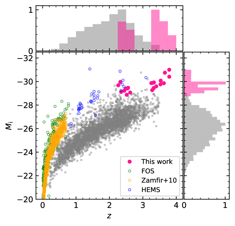
Figure 1: Location of the complete sample in the Hubble diagram (pink spots). Gray dots represent a random subsample of the DR16 catalogue from Lyke et al. (2020) and green, yellow, and blue dots represent the comparison samples defined in Section 2.2.

2.1 Redshift estimations and sample location in the Hubble diagram

Redshift measurements were based on the H$\beta$ emission line profile, and were obtained from the observed wavelength of the H$\beta$ narrow component (FWHM $\lesssim 1000$ km s^-1). The values are reported in Table 1. In the case of HE 0001-2340 and SDSSJ210831.56-063022.5 the redshift was estimated through the [O iii]$\lambda 5007$ emission line, due to the difficulty of isolating a narrow component of H$\beta$. Before performing the spectral analysis, described in section 4, both optical and UV spectra are set at rest-frame using the IRAF task dopcor.

Fig. 1 shows the location of the objects of the sample (pink spots) in the $i$-band absolute magnitude $M_{\rm{i}}$ vs. redshift plane. Our sample as well as the comparison samples (defined in Section 2.2) are located at the high end of the luminosity distribution when compared with the SDSS DR16 data (grey spots, Lyke et al. 2020). Moreover, some of our sources are well located within the region with the highest values of the SDSS redshift distribution for quasars.

2.2 Comparison samples

We have chosen comparison samples that include high- and low-redshift, as well as high- and low-luminosity sources that were studied in the recent literature, as follows:

• Low-$z$ SDSS sources: Zamfir et al. (2008) and Zamfir et al. (2010) analyse $\sim$ 470 low-redshift ($z\leq 0.7$) quasars with high signal-to-noise (S/N $\sim 29$) ratio optical spectra observed with the Sloan Digital Sky Survey data release (DR) 5 (Adelman-McCarthy et al., 2007), including both radio-loud and radio-quiet sources. This sample covers a wide range of bolometric luminosity, going from $\log L_{\rm{bol}}=10^{43}$ to $\log L_{\rm{bol}}=10^{47}$ erg s^-1.

• High-luminosity Hamburg-ESO sample (hereafter, HEMS): Sulentic et al. (2004, 2006b) and M09 obtained, using the VLT-ISAAC camera, H$\beta$ region measurements for a sample of 53 high-redshift high-luminosity objects, selected from the Hamburg-ESO survey. The sources are extremely luminous (47$\lesssim L_{\textrm{bol}}\lesssim$ 48) and are located in a redshift range of $0.9\lesssim z\lesssim 3.1$. We use these data as comparison sample at high $L$, for both H$\beta$ and [O III] lines. For the UV region we use the results provided by S17, who studied 28 quasars of the previous sample, and from which they obtained C IV$\lambda 1549$ observations with the VLT and TNG telescopes. The redshift range of the HEMS is $1.4\leq z\leq 3.1$ and a typical bolometric luminosity is $L_{\rm bol}\gtrsim 10^{47.5}$ erg s^-1. The location of the HEMS in the Hubble diagram is similar to the one of our data (Fig. 1) in terms of absolute magnitudes, although a large fraction of HE sources is with $1\lesssim z\lesssim 2$.

• Low-luminosity FOS data: The low-luminosity Faint Object Spectrograph (FOS) comparison sample was selected from Sulentic et al. (2007, S07 from now on), where the authors analysed the C IV line parameters. Marziani et al. (2003, hereafter M03) provide measurements on the H$\beta$ emission line for most sources in this sample. The typical bolometric luminosity of this sample is $\log L_{\rm{bol}}\sim 45.6$ [erg s^-1] and a redshift range $z\leq 0.5$.

3 Observations and Data

Table 2: Log of optical observations with VLT/ISAAC.

Source	Date obs.	Band	DIT	Nexp	Airmass	Averaged
	(start)		(s)		start-end	seeing
(1)	(2)	(3)	(4)	(5)	(6)	(7)
HE 0001-2340	2010-07-06	sH	180	12	1.05-1.02	1.03
	2010-07-24	sH	180	12	1.03-1.01	0.55
	2010-08-04	sH	180	12	1.06-1.12	1.44
$[\rm{HB89}]$ 0029+073	2009-09-03	sK	180	20	1.43-1.25	1.08
	2010-07-08	sK	180	20	1.25-1.19	0.49
	2010-08-04	sK	180	20	1.19-1.18	1.31
CTQ 0408	2009-07-09	sK	180	8	1.11-1.12	0.51
	2009-08-31	sK	180	8	1.11-1.12	3.05
SDSSJ005700.18+143737.7	2009-09-04	sH	180	28	1.44-1.98	1.99
H 0055-2659	2009-09-02	sK	180	40	1.01-1.23	1.25
SDSSJ114358.52+052444.9	2009-07-08	sH	180	20	1.34-1.67	0.83
SDSSJ115954.33+201921.1	2010-04-05	sK	175	24	2.35-1.69	1.08
SDSSJ120147.90+120630.2	2010-04-15	sK	180	20	1.92-1.49	1.23
SDSSJ132012.33+142037.1	2009-05-04	sH	180	24	1.36-1.28	1.37
SDSSJ135831.78+050522.8	2010-04-18	sH	180	20	1.23-1.18	0.73
Q 1410+096	2010-04-20	sK	180	28	1.45-1.23	0.83
SDSSJ141546.24+112943.4	2009-05-04	sH	180	20	1.24-1.26	0.50
B1422+231	2009-04-13	sK	180	12	1.50-1.48	0.98
SDSSJ153830.55+085517.0	2010-04-05	sK	180	20	1.20-1.24	1.14
SDSSJ161458.33+144836.9	2009-07-08	sH	180	20	1.33-1.30	1.35
	2009-09-22	sH	180	20	1.73-2.05	2.24
PKS 1937-101	2009-09-03	sK	180	12	1.13-1.23	1.07
PKS 2000-330	2009-08-31	sK	180	20	1.43-1.89	2.03
SDSSJ210524.49+000407.3	2010-07-23	sH	180	12	1.29-1.45	1.80
SDSSJ210831.56-063022.5	2010-06-19	sH	175	24	1.07-1.18	0.93
SDSSJ212329.46-005052.9	2010-07-08	sH	180	12	1.12-1.18	0.48
	2010-07-24	sH	180	12	1.41-1.27	0.90
PKS 2126-15	2009-09-01	sK	180	12	1.84-2.36	1.41
	2010-06-09	sK	180	16	1.26-1.12	1.07
SDSSJ235808.54+012507.2	2010-06-21	sK	180	20	1.25-1.13	1.01

3.1 Near Infrared Observations and data reduction

Spectra were taken in service mode in 2009 and 2010, with the infrared spectrometer ISAAC, mounted at the Nasmyth B focus of VLT-U1 (Antu) until August 2009, and later at the Nasmyth A focus of VLT-U3 (Melipal) at the ESO Paranal Observatory. Table 2 summarises the NIR observations, listing the date of observation (Col. 2), used grating (Col. 3), individual Detector Integration Time (DIT) in seconds (Col. 4), number of exposures with single exposure time equal to DIT (Col. 5), the range of air mass of the observations (Col. 6), and the averaged seeing (Col. 7). When the source was observed more than once (HE 0001-2340, [HB89] 0029+073, CTQ 0408, SDSSJ161458.33+144836.9, SDSSJ212329.46-005052.9, and PKS 2126-15), we combine the individual spectra to obtain a median weighted final spectrum for the analysis. Spectral resolutions are FWHM $=16$ Å in the $H$ band and FWHM $=22$ Å in the $K$ band.

Reductions were performed using standard IRAF routines. Several spectra of each source were taken, nodding the telescope between two positions (nodding amplitude = 20”). Each obtained frame was divided by the flat field provided by the ESO automated reduction pipeline. 1D spectra were extracted using the IRAF program “apall”. Cosmic ray hits were eliminated by interpolation using a median filter, comparing the affected spectrum with the other spectra of the same source.

For each position along the slit, a 1D xenon/argon arc spectrum was extracted from the calibration lamp frame, using the same extraction parameters as the corresponding target spectrum. The wavelength calibration was well modeled by 3rd order Chebyshev polynomial fits to the positions of 15-30 lines, with rms residuals of 0.3 Å in sH and 0.6 Å in sK. The wavelength calibration is usually affected by a small 0-order offset caused by grism and telescope movement, because the arc lamp frames were obtained in daytime. A correction for these shifts was obtained by measuring the centroids of 2–3 OH sky against the arc calibration and calculating the average difference, which reached at most 2-3 pixels in either direction. Once matched with the corresponding arc calibrations, the individual spectra of each source were rebinned to a common linear wavelength scale and stacked.

The spectra of the atmospheric standard stars were extracted and wavelength-calibrated in the same way. All clearly identifiable stellar features (H and HeI absorption lines) were eliminated from the stellar spectra by spline interpolation of the surrounding continuum intervals. Each target spectrum was then divided by its corresponding standard star spectrum in order to correct for the atmospheric absorption features. This was achieved with the IRAF routine “telluric”, which allows to optimise the correction with slight adjustments in shift and scaling of the standard spectrum. The correct flux calibration of each spectrum was achieved by scaling it according to the magnitude of the standard star and to the ratio of the respective DITs. Because the seeing often exceeded the width of the slit, significant light loss occurred, and therefore the absolute flux scale of the spectra is not to be considered as accurate. However, in this long-wavelength range we consider the light losses to be independent of wavelength (i.e., we assume that differential atmospheric refraction is negligible), and they should therefore not affect the relative calibration of the spectra. We carried out an a posteriori evaluation of the absolute flux calibration uncertainty performing a comparison between the $H/K$-band magnitudes estimated by convolving the $H/K$ filter with the observed spectrum and the $H/K$ magnitudes in NED. The differences are smaller than 0.5 mag, except for SDSSJ132012.33+142037.1, SDSSJ141546.24+112943.4, and SDSSJ153830.55+085517.0 where a correction factor $\sim 0.880\pm 0.176$ mag was applied.

Table 3: UV spectra information.

Source	UV	Comments
	Spect.
(1)	(2)	(3)
SDSSJ005700.18+143737.7	BOSS
SDSSJ114358.52+052444.9	BOSS
SDSSJ115954.33+201921.1	SDSS
SDSSJ120147.90+120630.2	BOSS
SDSSJ132012.33+142037.1	BOSS
SDSSJ135831.78+050522.8	BOSS
Q 1410+096	SDSS	BAL
SDSSJ141546.24+112943.4	SDSS	BAL
SDSSJ153830.55+085517.0	BOSS	BAL(a)
SDSSJ161458.33+144836.9	BOSS
PKS 2000-330	Barthel et al. (1990)
SDSSJ210524.49+000407.3	SDSS	BAL
SDSSJ210831.56-063022.5	SDSS
SDSSJ212329.46-005052.9	BOSS
SDSSJ235808.54+012507.2	BOSS

3.2 UV

We have found useful UV spectra (i.e., which include at least one of the three UV regions of our interest) for the 15/22 sources that are listed in Table 3, where we also list in Col. 2 the database/reference from which each spectrum was obtained and in Col. 3 the Broad Absorption Lines (BAL) quasars. We report the BAL sources as the analysis of the region in which the broad absorptions are located should be taken with care, once it demands the addition of absorption components in the fitting routine. The other seven quasars do not have useful UV spectra, either because they are old spectra not digitally available and have low S/N not suitable for accurate profile fitting, or because they do not include any of the three UV regions we want to analyse (Si IV$\lambda$1397+O IV$\lambda$1402, C IV$\lambda$1549+He II$\lambda$1640, and the 1900 Å blend). For the UV spectral range (observed in the optical domain at the redshift of this sample), the spectra were collected mainly from the SDSS DR16 database (Ahumada et al., 2020, and references therein). For one source (PKS 2000-330), the UV spectrum was digitalized from Barthel et al. (1990). Four out of the 22 quasars (Q 1410+096, SDSSJ141546.24+112943.4, SDSSJ153830.55+085517.0 and SDSSJ210524.49+000407.3) are classified as BAL quasars, due to strong absorption lines (Gibson et al., 2009; Scaringi et al., 2009; Allen et al., 2011; Welling et al., 2014; Bruni et al., 2019; Yi et al., 2020).

3.3 Radio data

The radio fluxes presented in Table 1 were collected from the 1.4-GHz NRAO VLA Sky Survey (NVSS, Condon et al. (1998)) and from the VLA FIRST Survey (Gregg et al., 1996; Becker et al., 1995). The flux in radio is reported for seven of our sources and in the case the object is not detected we provide an upper limit to the flux, which corresponds to the detection limit ($\approx$ 5 times the rms in both FIRST and NVSS catalogue) at the position of the source. In the case of CTQ 0408, there is no coverage either in the FIRST survey or in the NVSS survey. The radio flux for this source is obtained at 408MHz from the Sidney University Molonglo Sky Survey catalogue (Mauch et al., 2003). The radio classification is shown in Col. 12 of Table 1 and it was determined following Ganci et al. (2019) through the estimation of a modified rest-frame radio loudness parameter $R_{\rm{K}}={f_{\rm{\nu,radio}}/f_{\rm{\nu,optical}}}$ (Kellermann et al., 1989), defined as the ratio between the specific flux at 1.4 GHz and in the $g$-band. Accordingly, our sample is separated into three different ranges: radio-quiet (RQ; $R_{\rm{K}}<10$), radio-intermediate (RI; $10\leq R_{\rm{K}}<70$), and radio-loud (RL; $R_{\rm{K}}\geq 70$). Of the seven sources with radio detection, three of them (CTQ 0408, SDSSJ141546.24+112943.4, and SDSSJ210524.49+000407.3) are classified as radio-intermediate. The radio-loud sources from our sample are B1422+231, PKS 1937-101, PKS 2000-330, and PKS 2126-15, about 20% of the sources of this sample. We plan to carry out in a forth-coming paper a similar spectroscopic study focused on RL quasars, to supplement those listed in Table 1.

4 Spectral Analysis

4.1 Optical range: multicomponent fitting

4.1.1 H$\beta$

The multicomponent fits were performed, after the spectra were set at rest-frame, using the specfit routine from IRAF (Kriss, 1994). This routine allows for simultaneous minimum-$\chi^{2}$ fit of the continuum approximated by a power-law and the spectral line components yielding FWHM, peak wavelength, and intensity of all line components. In the optical range we fit the H$\beta$ profile as well as the [O III]$\lambda\lambda 4959,5007$ emission lines and the Fe II multiplets for the 22 objects.

Our approach includes the continuum (a power law), a semi-empirical scalable Fe II emission template and the emission line components to fit the H$\beta$+[O III]$\lambda\lambda 4959,5007$ region. The Fe II template used is almost identical to the one of Boroson & Green (1992). The specfit routine allows for the scaling, broadening, and shifting of the Fe II template to model the observed features (Marziani et al., 2003).

A sketch to illustrate the decomposition approach performed on the fittings of emission lines broad profiles is presented in Fig. 2. The fit of the H$\beta$ full profile takes into account three main components:

• Broad component (BC): this component is kept symmetric, set almost always at rest-frame, and presents a FWHM range that goes from $\gtrsim 3000$ km s^-1 for some Pop. A and $\lesssim 6000$ km s^-1 for Pop. B quasars. The profile changes depending on the quasar population, presenting a Lorentzian-like shape for Pop. A and a Gaussian-like one for Pop. B sources (Sulentic et al., 2002; Marziani et al., 2003; Zamfir et al., 2010; Cracco et al., 2016);

• Blueshifted component (BLUE): our first assumption is to model this component by only a blue-shifted Gaussian (symmetric or skewed) profile with FWHM and shift similar to the [O III]$\lambda\lambda$4959,5007 semi-broad component (SBC, explained in §4.1.2). When the H$\beta$ profile does not correspond to the blueshifted SBC of [O III]$\lambda\lambda$4959,5007 profile, it is included in the fitting an additional Gaussian blue-shifted component that may not belong to NLR emission (BLUE). BLUE is believed, unlike the SBC, to be associated with emission of outflowing gas from within the BLR (Negrete et al., 2018);

• Very broad component (VBC): it is clearly observed in Population B sources (Sulentic et al., 2017; Wolf et al., 2020). It is always represented by a redshifted Gaussian profile and it is thought to be related with the high-ionisation virialised region closest to the continuum source (Peterson & Ferland, 1986; Snedden & Gaskell, 2007; Wang & Li, 2011). This component can easily achieve FWHM $\gtrsim$ 10000 km s^-1.

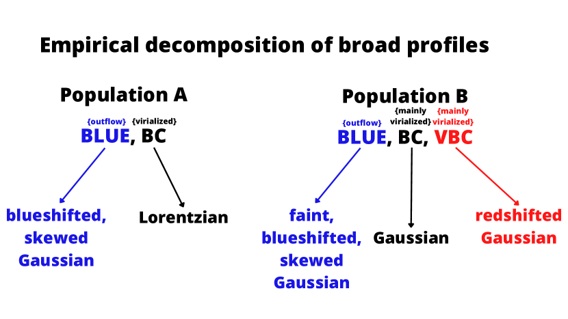
Figure 2: Sketch of the approach followed for broad profile fittings.

In addition, we include a narrow component (NC) superimposed to the broad emission line profile and it is fitted as an unshifted Gaussian.

The Population classification depends on the FWHM of the full profile. Depending on the population assignment, different components are included and they assume different line shapes. An exhaustive analysis of the fittings were performed and in borderline cases (i.e., with line width close to the boundary between Pop. A and B), the final conclusion on the population of the source is based on the $\chi^{2}$ of the fitting (i.e., the fittings with the minimum $\chi^{2}$ are selected).

4.1.2 [O III]$\lambda\lambda$4959,5007

An approach similar to the one used for H$\beta$ is also followed for the [O III]$\lambda\lambda 4959,5007$ emission line profiles. The [O III]$\lambda\lambda 4959,5007$ full profile is assumed to be well represented by a Gaussian narrow (FWHM $\lesssim 1200$ km s^-1) component set at rest-frame or shifted to the blue and a semi-broad component (SBC, FWHM typically $\lesssim 3000$ km s^-1) that usually appears more shifted to the blue ($\sim$ 1000 km/s, Zhang et al., 2011; Marziani et al., 2016b, 2022b). The NC is modelled as a Gaussian profile for the two populations and in a first approach the NC of both H$\beta$ and [O III]$\lambda\lambda$4959,5007 share the same line width. The blueshifted contributions can be modelled by one or more Gaussian profiles and in some cases the Gaussian needs to be asymmetric towards the blue to account for the line shape, i.e., to be a skewed Gaussian. The use of a skewed Gaussian has a physical motivation, as it might be associated with bipolar outflow emission in which the receding side of the outflow is obscured. Apart from that, both [O iii]$\lambda 4959$ and [O iii]$\lambda 5007$ emission line profiles are assumed to have the same FWHM and shifts, and the intensity ratio between the two lines is kept fixed at 1:3 (Dimitrijević et al., 2007).

4.2 UV range: multicomponent fitting

Fits are performed for three different regions centred on Si IV$\lambda 1397$+O IV]$\lambda 1402$, C IV$\lambda 1549$+He II$\lambda 1640$, and the 1900 Å blend that includes the Al III$\lambda 1860$ doublet, Si III]$\lambda 1892$, Si II $\lambda 1816$, and C III]$\lambda 1909$. UV fittings are presented for 15 sources. The fits were not carried out in cases where the emission lines are strongly affected by BALs. The fittings of the absorption lines are performed in sources in which the presence of these lines allows to clearly see the emission line profile (as in the case of mini-BALs; Sulentic et al. 2006a). The UV blends are fit following the population assignments from the H$\beta$ spectral range. The only exception is SDSSJ153830.55+085517.0, where its UV spectrum cannot be fitted in agreement with its classification as Pop. B in the H$\beta$ region, as highlighted in the Appendix A.

4.2.1 1900 Å blend

In the UV region corresponding to the 1900 $\AA$ blend, the fittings are performed considering the Al III$\lambda 1860$ doublet, Si III]$\lambda 1892$, Si II $\lambda 1816$, and C III]$\lambda 1909$ emission line profiles. Fe III is especially relevant on the red side of the 1900 Å blend and its modelling has been performed using the Vestergaard & Wilkes (2001) empirical template, and following the same approach as for the optical Fe II. Broad line components of the 1900 Å blend in Pop. A sources are fitted by Lorentzian profiles while in Pop. B by Gaussian functions (as is the case of H$\beta$ in the optical spectral range), keeping the same (or at least a comparable) FWHM to the broad component of H$\beta$.

In several Pop. A and more frequently in xA quasars, the Fe III template and the C III]$\lambda 1909$ broad component do not reproduce well the shape of the red side of the 1900 Å blend. A better model of the C III]$\lambda 1909$ region is achieved assuming an additional contribution mostly likely due to the Fe III line at 1914Å. The same approach was employed in Martínez-Aldama et al. (2018).

Regarding the Pop. B sources, the C III]$\lambda 1909$ emission line is well represented by the same combination applied for Pop. B H$\beta$: VBC+BC+NC. The VBC FWHM is expected to be $\geq 4000$ km s^-1, and the NC FWHM $\sim 1000$ km s^-1 (there is only one source that shows a significant NC in C III]). Differently from C III]$\lambda 1909$, lines such as the Al III$\lambda 1860$ doublet, Si III]$\lambda 1892$, and Si II $\lambda 1816$ are assumed not to present a very broad component (Buendia-Rios et al., 2022). They are fit by only one BC.

4.2.2 C IV$\lambda 1549$+He II$\lambda 1640$

In order to fit the C IV$\lambda 1549$+He II$\lambda 1640$ blend and contaminant lines within it, we use the approach followed by S17. As in the previous fits, we represent Pop. A profiles of C IV$\lambda 1549$ and He II$\lambda 1640$ by a broad and a blueshifted component. Pop. B are represented by the combination VBC+BC+BLUE. The broad components of C IV$\lambda 1549$ and He II$\lambda 1640$ are fixed at rest-frame and the other components are left free to vary in wavelength. Nevertheless, the FWHM and shapes of He II$\lambda 1640$ BC and BLUE are restricted to be equal (or comparable) to the corresponding ones of C IV$\lambda 1549$. These constraints are physically motivated since both C IV$\lambda$1549 and He II$\lambda$1640 are expected to be emitted from the same regions, because of the similar ionisation potential of the parent ionic species. An additional condition is that the broad component (BC) of C IV$\lambda$1549 and He II$\lambda 1640$ FWHM should be equal or larger to the one of H$\beta$, following previous works (e.g. Sulentic et al., 2017, and references therein).

4.2.3 Si IV$\lambda 1397$+O IV]$\lambda 1402$

For the Si IV$\lambda 1397$+O IV]$\lambda 1402$ emission lines region, we follow the same steps as in the C IV+He II blend. The Si IV$\lambda 1397$+O IV]$\lambda 1402$ feature profile is similar to the one of C IV$\lambda 1549$, and is therefore expected to present BC and blueshifted component similar to those of C IV$\lambda 1549$. The broad component in this case is also kept at rest-frame and any other necessary component is free to change in all the parameters.

4.3 Analysis of the full profile parameters for the optical and UV regions

Apart from the multicomponent analysis, the H$\beta$ and [O III] emission line profiles are also characterised through the parametrisation of the full profile by measuring centroids and widths at different fractional intensities (1/4, 1/2, 3/4, and 9/10), as well as asymmetry and kurtosis indexes in order to provide a quantitative description independent of the specfit modelling. In the case of H$\beta$, the full profile (H$\beta_{\textrm{full}}$) for Pop. B quasars is represented by BC+VBC plus BLUE when detected. For Pop. A quasars, full H$\beta$ profile consists of BC plus BLUE if an additional blue component is present. For [O iii] we consider NC and one (or more, if needed) blueshifted SBC. Full profile parameters for the UV region are provided for the C IV$\lambda$1549 broad emission line, excluding NC.

4.4 Error estimates

Uncertainties in the multicomponent fits were estimated by running Markov Chain Monte Carlo (MCMC) simulations, following the approach described in Marziani et al. (2022c) for both optical and UV spectral ranges. Observed spectra were modeled using the components employed in the best fit, with a Markov Chain to sample the domain around the minimum $\chi^{2}$. The dispersion in the posterior distribution of a parameter was assumed to be its 1$\sigma$ confidence interval. For the optical range, the errors are around the order of 10% for the FWHM of the H$\beta_{\rm{BC}}$ and [O III]_SBC. Larger uncertainties ($\sim 30\%$) are found for the narrow components of both lines and for the blueshifted component of H$\beta$. Flux uncertainties for strong or sharp emission lines are $\sim 10\%$, while typical errors for the continuum and Fe II are $\sim 5\%$ and $\sim 15\%$  respectively, if Fe II is reasonably strong.

For the UV, the FWHM uncertainties are between 10% and 15% and errors on intensity measurements are usually $\lesssim 10\%$ for the strongest emission line components.

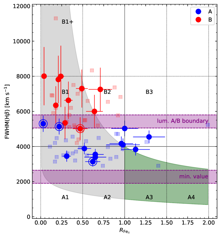
Figure 3: Location of our sources through the optical plane of the 4DE1. Pop. A quasars are represented by blue circles and Pop. B by red circles. The radio-loud sources from the sample are surrounded by a circle in the plot. Grey and green regions indicate the distribution of the Main Sequence of quasars across the 4DE1 optical plane in a low-$z$ context (Marziani et al., 2018). Spectral Types (ST) of the MS are labelled according to Sulentic et al. (2002). Blue and red squares indicate high-redshift Pop. A and Pop. B quasars from M09, respectively. Purple-shaded areas show the luminosity-dependent boundary between Pops. A and B and the minimum FWHM value for sources with $47\leq L_{\mathrm{bol}}\leq 48$ and assuming $\alpha=0.67$ (Marziani et al., 2009).

5 Results

5.1 Location in the optical plane of Main Sequence

After performing the multicomponent fitting, we can locate the sample in the MS optical plane, using the FWHM(H$\beta_{\rm full}$) as well as the flux ratio of Fe II$\lambda$4570 and H$\beta$, $R_{\mathrm{{Fe\textsc{II}}}}$. Fig. 3 shows the location of the sources and a comparison between our sample and low- and high-$z$ samples. The grey- and green-shaded areas in the plot indicate the location of low-redshift quasars on the MS, with the xA sources situated on the green shadow.

Our sample shows a slight displacement in the direction of increasing FWHM(H$\beta$), if compared to low-$z$ samples (e.g., Zamfir et al., 2010, and the shaded area in Fig. 3). There are some Pop. A sources that present a FWHM(H$\beta_{\rm{full}}$) $\sim 5000$ km s^-1. The Pop. A/B boundary at FWHM(H$\beta$) $=4000$ km s^-1 is reasonable when considering low redshift and, consequently, lower luminosity ranges than those of high-$z$ quasars (Sulentic et al., 2004). However, at high luminosity there is a significant effect on the H$\beta$ profile width that may shift the boundary between Pop. A and B by more than 1000 km s^-1 (M09). Up and bottom purple shadows in Fig. 3 indicate, respectively, the Pop. A/B boundary and the minimum FHWM(H$\beta$) found in a $47\leq\log L_{\rm{bol}}\leq 48$ range, representative of our sample. Both boundaries were determined following M09.

From the 22 sources of our sample, 12 are classified as Pop. A and 10 as Pop. B quasars. We found three sources to belong to spectral type (ST) A1; six Pop. A2; three Pop. A3 (extreme A); eight to be Pop. B1; and two Pop B2. The four radio-loud objects (B1422+231, PKS 1937-101, PKS 2000-330, and PKS 2126-15) are identified in Figure 3 by the blue and red symbols surrounded by a open circle. Three of them are classified as Pop. A and only PKS 2126-15 is a Pop. B quasar. Of the three radio-intermediate, two (SDSSJ141546.24+112943.4, ST B2; SDSSJ210524.49+000407.3, A3) show significant Fe II and an overall spectrum associated with high accretion rates (Ganci et al., 2019; del Olmo et al., 2021; Marziani et al., 2022a). Only CTQ 0408 is classified as B1, with an optical spectrum resembling the powerful jetted sources at low $z$. The orientation may strongly affect the classification of the sources, especially in the cases when the FWHM(H$\beta$) is at the border line of the A/B boundary. Orientation effects could be particularly important in the case of core-dominated RL sources, as the pole-on orientation may imply a narrowing of low-ionization emission line widths (Wills & Browne, 1986; Marziani et al., 2001; Sulentic et al., 2003; Rokaki et al., 2003; Zamfir et al., 2008; Bisogni et al., 2017).

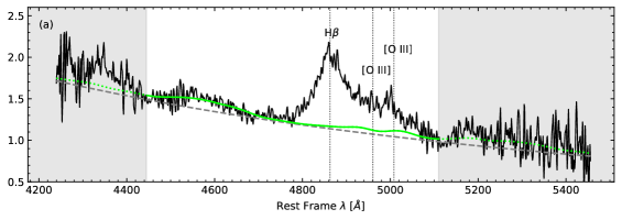
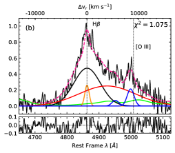
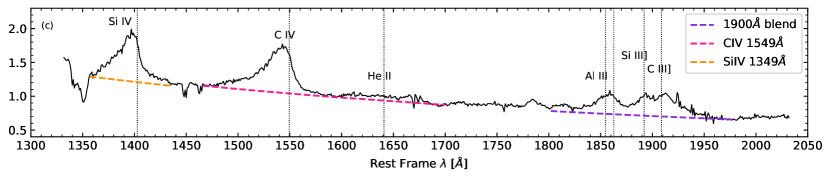
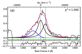
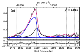
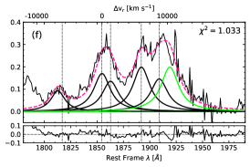
Figure 31: SDSSJ153830.55+085517.0. Same as Figure 23.

There is just one case of a blatant disagreement between the classification deduced from the optical and UV spectra of the same source: SDSSJ153830.55+085517.0, which is optically classified as Pop. B but presents clearly Pop. A-like profiles in the UV spectrum (see §A.14 and Fig. 31 in the Appendix A). In this case it was necessary to fit the optical as Pop. B and the UV as Pop. A.

Table 4: Spectrophotometric measurements on H$\beta$.

Source	Spectral	$f_{\lambda,5100}$ (a)	$W$(H$\beta$)	$W$([O III])	$R_{{Fe\textsc{II}}}$
	Type			[Å]
(1)	(2)	(3)	(4)	(5)	(6)
Population A
SDSSJ005700.18+143737.7	A3	2.5 $\pm$ 0.3	53 $\pm$ 6	4.5 $\pm$ 0.5	1.13 $\pm$ 0.17
SDSSJ132012.33+142037.1	A1	1.2 $\pm$ 0.1	74 $\pm$ 9	19.8 $\pm$ 2.4	0.31 $\pm$ 0.05
SDSSJ135831.78+050522.8	A2	2.2 $\pm$ 0.3	68 $\pm$ 8	16.3 $\pm$ 2.0	0.65 $\pm$ 0.10
Q 1410+096	A2	3.0 $\pm$ 0.4	57 $\pm$ 7	13.7 $\pm$ 1.6	0.65 $\pm$ 0.13
B1422+231	A1	4.0 $\pm$ 0.5	78 $\pm$ 9	9.3 $\pm$ 1.1	0.22 $\pm$ 0.03
SDSSJ161458.33+144836.9	A2	2.3 $\pm$ 0.3	83 $\pm$ 9	16.8 $\pm$ 2.0	0.52 $\pm$ 0.08
PKS 1937-101	A1	7.6 $\pm$ 0.9	62 $\pm$ 7	13.5 $\pm$ 1.6	0.03 $\pm$ 0.01
PKS 2000-330	A2	2.8 $\pm$ 0.3	59 $\pm$ 7	15.1 $\pm$ 1.8	0.62 $\pm$ 0.09
SDSSJ210524.49+000407.3	A3	3.9 $\pm$ 0.5	31 $\pm$ 4	0.4 $\pm$ 3.0	1.00 $\pm$ 0.16
SDSSJ210831.56-063022.5	A3	1.4 $\pm$ 0.2	44 $\pm$ 6	4.7 $\pm$ 0.6	1.29 $\pm$ 0.19
SDSSJ212329.46-005052.9	A2	4.4 $\pm$ 0.5	34 $\pm$ 5	5.5 $\pm$ 0.7	0.96 $\pm$ 0.14
SDSSJ235808.54+012507.2	A2	4.7 $\pm$ 0.6	63 $\pm$ 8	10.7 $\pm$ 1.3	0.98 $\pm$ 0.20
Population B
HE 0001-2340	B1	1.6 $\pm$ 0.2	77 $\pm$ 9	10.6 $\pm$ 1.3	0.33 $\pm$ 0.05
$[\rm HB89]$ 0029+073	B1	2.4 $\pm$ 0.3	62 $\pm$ 7	7.8 $\pm$ 0.9	0.18 $\pm$ 0.02
CTQ 408	B1	6.9 $\pm$ 0.8	53 $\pm$ 6	2.5 $\pm$ 4.0	0.49 $\pm$ 0.07
H 0055-2659	B1	1.9 $\pm$ 0.2	92 $\pm$ 11	40.6 $\pm$ 4.9	0.29 $\pm$ 0.03
SDSSJ114358.52+052444.9	B2	1.1 $\pm$ 0.1	82 $\pm$ 10	5.4 $\pm$ 0.6	0.64 $\pm$ 0.10
SDSSJ115954.33+201921.1	B1	2.5 $\pm$ 0.3	78 $\pm$ 9	15.2 $\pm$ 1.8	0.04 $\pm$ 0.01
SDSSJ120147.90+120630.2	B1	4.3 $\pm$ 0.5	117 $\pm$ 14	21.0 $\pm$ 2.5	0.24 $\pm$ 0.04
SDSSJ141546.24+112943.4	B2	2.1 $\pm$ 0.3	108 $\pm$ 13	33.9 $\pm$ 4.1	0.71 $\pm$ 0.14
SDSSJ153830.55+085517.0	B1	1.1 $\pm$ 0.1	94 $\pm$ 11	5.5 $\pm$ 0.7	0.21 $\pm$ 0.03
PKS 2126-15	B1	4.8 $\pm$ 0.6	93 $\pm$ 11	10.0 $\pm$ 1.2	0.47 $\pm$ 0.09

Table 5: Results from specfit analysis on H$\beta$.

	H$\beta$ full broad profile							Full broad profile (BLUE+BC+VBC)															Narrow profile (SBC+NC)
											BLUE(a)				BC				VBC						SBC				NC
Source	FWHM	A. I.	Kurt.	c($\frac{1}{4}$)	c($\frac{1}{2}$)	c($\frac{3}{4}$)	c($\frac{9}{10}$)		$I_{\mathrm{tot}}^{(b)}$		$I/I_{\mathrm{tot}}$	FWHM	Shift		$I/I_{\mathrm{tot}}$	FWHM	Shift		$I/I_{\mathrm{tot}}$	FWHM	Shift		$I_{\mathrm{tot}}^{(c)}$		$I/I_{\mathrm{tot}}$	FWHM	Shift		$I/I_{\mathrm{tot}}$	FWHM	Shift
	[km s-1]			[km s-1]	[km s-1]	[km s-1]	[km s-1]					[km s-1]	[km s-1]			[km s-1]	[km s-1]			[km s-1]	[km s-1]					[km s-1]	[km s-1]			[km s-1]	[km s-1]
(1)	(2)	(3)	(4)	(5)	(6)	(7)	(8)		(9)		(10)	(11)	(12)		(13)	(14)	(15)		(16)	(17)	(18)		(19)		(20)	(21)	(22)		(23)	(24)	(25)
Population A
SDSSJ005700.18+143737.7	3830 $\pm$ 342	-0.09 $\pm$ 0.01	0.33 $\pm$ 0.01	-359 $\pm$ 237	-326 $\pm$ 83	-137 $\pm$ 107	-82 $\pm$ 118		1.66 $\pm$ 0.20		0.08 $\pm$ 0.03	2562 $\pm$ 359	-2154 $\pm$ 548		0.92 $\pm$ 0.06	3255 $\pm$ 346	0 $\pm$ 10		…	…	…		1.89 $\pm$ 0.23		0.00	…	…		1.00 $\pm$ 0.32	873 $\pm$ 93	0 $\pm$ 10
SDSSJ132012.33+142037.1	3450 $\pm$ 314	-0.11 $\pm$ 0.03	0.31 $\pm$ 0.01	-476 $\pm$ 323	-215 $\pm$ 72	-138 $\pm$ 93	-125 $\pm$ 110		0.91 $\pm$ 0.11		0.12 $\pm$ 0.05	7519 $\pm$ 1053	-1745 $\pm$ 584		0.88 $\pm$ 0.05	3224 $\pm$ 343	-41 $\pm$ 14		…	…	…		1.13 $\pm$ 0.14		0.00	…	…		1.00 $\pm$ 0.32	623 $\pm$ 66	-22 $\pm$ 17
SDSSJ135831.78+050522.8	3548 $\pm$ 314	0.00 $\pm$ 0.12	0.33 $\pm$ 0.01	-1 $\pm$ 297	0 $\pm$ 60	0 $\pm$ 97	0 $\pm$ 120		1.58 $\pm$ 0.19		0.00	…	…		0.92 $\pm$ 0.06	3548 $\pm$ 377	0 $\pm$ 10		…	…	…		1.49 $\pm$ 0.18		1.00 $\pm$ 0.32	5497 $\pm$ 770	-1712 $\pm$ 572		0.00	…	…
Q 1410+096	3394 $\pm$ 299	0.00 $\pm$ 0.08	0.33 $\pm$ 0.01	54 $\pm$ 279	54 $\pm$ 58	54 $\pm$ 92	54 $\pm$ 112		1.79 $\pm$ 0.21		0.00	…	…		1.00 $\pm$ 0.06	3394 $\pm$ 361	54 $\pm$ 58		…	…	…		0.37 $\pm$ 0.04		1.00 $\pm$ 0.32	4581 $\pm$ 320	-3144 $\pm$ 1051		0.00	…	…
B1422+231	5136 $\pm$ 452	0.00 $\pm$ 0.06	0.33 $\pm$ 0.01	-1 $\pm$ 422	-1 $\pm$ 89	0 $\pm$ 139	0 $\pm$ 169		3.20 $\pm$ 0.38		0.00	…	…		1.00 $\pm$ 0.06	5135 $\pm$ 546	0 $\pm$ 10		…	…	…		0.57 $\pm$ 0.07		0.00	…	…		1.00 $\pm$ 0.32	1113 $\pm$ 118	0 $\pm$ 10
SDSSJ161458.33+144836.9	3885 $\pm$ 349	-0.06 $\pm$ 0.11	0.33 $\pm$ 0.01	-241 $\pm$ 327	-98 $\pm$ 73	-51 $\pm$ 106	-38 $\pm$ 130		1.89 $\pm$ 0.21		0.09 $\pm$ 0.03	7224 $\pm$ 506	-1713 $\pm$ 571		0.91 $\pm$ 0.06	3721 $\pm$ 396	0 $\pm$ 10		…	…	…		0.54 $\pm$ 0.06		0.70 $\pm$ 0.25	2445 $\pm$ 170	-1709 $\pm$ 569		0.30 $\pm$ 0.09	439 $\pm$ 47	0 $\pm$ 10
PKS 1937-101	5298 $\pm$ 466	0.00 $\pm$ 0.07	0.33 $\pm$ 0.01	56 $\pm$ 434	56 $\pm$ 92	56 $\pm$ 144	56 $\pm$ 174		5.15 $\pm$ 0.62		0.00	…	…		1.00 $\pm$ 0.06	5296 $\pm$ 563	56 $\pm$ 92		…	…	…		1.57 $\pm$ 0.19		0.29 $\pm$ 0.09	2618 $\pm$ 183	-555 $\pm$ 183		0.71 $\pm$ 0.22	852 $\pm$ 91	-47 $\pm$ -77
PKS 2000-330	3230 $\pm$ 294	-0.06 $\pm$ 0.07	0.32 $\pm$ 0.01	-175 $\pm$ 306	-30 $\pm$ 61	1 $\pm$ 89	9 $\pm$ 108		1.92 $\pm$ 0.22		0.05 $\pm$ 0.01	5499 $\pm$ 385	-3127 $\pm$ 1031		0.95 $\pm$ 0.06	3138 $\pm$ 334	28 $\pm$ 54		…	…	…		2.31 $\pm$ 0.28		0.36 $\pm$ 0.11	1499 $\pm$ 105	-599 $\pm$ 197		0.63 $\pm$ 0.20	1082 $\pm$ 115	-46 $\pm$ -89
SDSSJ210524.49+000407.3	5026 $\pm$ 446	0.00 $\pm$ 0.06	0.33 $\pm$ 0.01	-1 $\pm$ 420	0 $\pm$ 85	0 $\pm$ 137	0 $\pm$ 169		1.28 $\pm$ 0.15		0.00	…	…		1.00 $\pm$ 0.06	5026 $\pm$ 534	0 $\pm$ 10		…	…	…		0.40 $\pm$ 0.05		0.00	…	…		1.00 $\pm$ 0.32	1407 $\pm$ 150	0 $\pm$ 10
SDSSJ210831.56-063022.5	4545 $\pm$ 200	0.00 $\pm$ 0.04	0.33 $\pm$ 0.01	93 $\pm$ 372	93 $\pm$ 79	93 $\pm$ 124	93 $\pm$ 149		0.60 $\pm$ 0.08		0.00	…	…		0.91 $\pm$ 0.06	4543 $\pm$ 483	93 $\pm$ 16		…	…	…		0.68 $\pm$ 0.08		0.89 $\pm$ 0.28	2597 $\pm$ 364	-2018 $\pm$ 347		0.11 $\pm$ 0.03	1403 $\pm$ 149	0 $\pm$ 10
SDSSJ212329.46-005052.9	4165 $\pm$ 366	0.00 $\pm$ 0.03	0.33 $\pm$ 0.01	-1 $\pm$ 342	-1 $\pm$ 72	0 $\pm$ 200	-1 $\pm$ 231		1.60 $\pm$ 0.22		0.00	…	…		0.89 $\pm$ 0.05	4164 $\pm$ 443	0 $\pm$ 10		…	…	…		2.40 $\pm$ 0.29		0.86 $\pm$ 0.27	4969 $\pm$ 696	-1844 $\pm$ 323		0.14 $\pm$ 0.04	1188 $\pm$ 126	0 $\pm$ 10
SDSSJ235808.54+012507.2	4098 $\pm$ 360	0.03 $\pm$ 0.06	0.35 $\pm$ 0.01	0 $\pm$ 336	0 $\pm$ 70	0 $\pm$ 111	-1 $\pm$ 136		2.88 $\pm$ 0.35		0.00	…	…		1.00 $\pm$ 0.06	4098 $\pm$ 436	0 $\pm$ 10		…	…	…		3.76 $\pm$ 0.45		0.38 $\pm$ 0.12	2463 $\pm$ 172	-1030 $\pm$ 340		0.61 $\pm$ 0.19	954 $\pm$ 101	0 $\pm$ 10
Median	3991 $\pm$ 1141	0.00 $\pm$ 0.06	0.33 $\pm$ 0.01	-1 $\pm$ 205	-0.5 $\pm$ 61	0 $\pm$ 27	0 $\pm$ 51		1.72 $\pm$ 0.65		0.08 $\pm$ 0.02	6362 $\pm$ 2533	-1949 $\pm$ 660		0.93 $\pm$ 0.09	3909 $\pm$ 1305	0$\pm$ 34		…	…	…		1.31 $\pm$ 1.43		0.78 $\pm$ 0.54	2607 $\pm$ 2219	-1710 $\pm$ 965		0.67 $\pm$ 0.62	1018 $\pm$ 312	0 $\pm$ 16
Population B
HE 0001-2340	6632 $\pm$ 1065	0.16 $\pm$ 0.22	0.37 $\pm$ 0.01	1757 $\pm$ 873	1134 $\pm$ 153	960 $\pm$ 354	909 $\pm$ 471		1.30 $\pm$ 0.16		0.00	…	…		0.42 $\pm$ 0.06	5063 $\pm$ 366	681 $\pm$ 92		0.58 $\pm$ 0.06	10982 $\pm$ 1955	2538 $\pm$ 342		0.33 $\pm$ 0.04		0.34 $\pm$ 0.11	3772 $\pm$ 264	-414 $\pm$ 136		0.65 $\pm$ 0.21	1067 $\pm$ 77	0 $\pm$ 10(d)
$[\rm HB89]$ 0029+073	6347 $\pm$ 1085	0.18 $\pm$ 0.05	0.37 $\pm$ 0.01	932 $\pm$ 757	292 $\pm$ 138	51 $\pm$ 339	-19 $\pm$ 442		1.54 $\pm$ 0.18		0.07 $\pm$ 0.01	4995 $\pm$ 837	-1216 $\pm$ 575		0.33 $\pm$ 0.05	4508 $\pm$ 326	-310 $\pm$ 147		0.60 $\pm$ 0.06	9609 $\pm$ 1710	1430 $\pm$ 193		1.54 $\pm$ 0.18		0.00	…	…		1.00 $\pm$ 0.32	1024 $\pm$ 74	0 $\pm$ 10
CTQ 408	7301 $\pm$ 1081	0.10 $\pm$ 0.09	0.40 $\pm$ 0.02	724 $\pm$ 910	306 $\pm$ 179	197 $\pm$ 390	164 $\pm$ 528		3.90 $\pm$ 0.47		0.00	…	…		0.52 $\pm$ 0.08	6050 $\pm$ 437	0 $\pm$ 10		0.48 $\pm$ 0.05	13243 $\pm$ 2357	1963 $\pm$ 264		2.54 $\pm$ 0.30		0.00	…	…		1.00 $\pm$ 0.32	1500 $\pm$ 108	0 $\pm$ 10
H 0055-2659	5342 $\pm$ 925	0.36 $\pm$ 0.13	0.30 $\pm$ 0.03	2249 $\pm$ 1085	580 $\pm$ 101	380 $\pm$ 283	329 $\pm$ 377		1.85 $\pm$ 0.22		0.00	…	…		0.27 $\pm$ 0.04	4609 $\pm$ 333	-224 $\pm$ 39		0.73 $\pm$ 0.07	13355 $\pm$ 2377	2527 $\pm$ 340		0.82 $\pm$ 0.10		0.00	…	…		1.00 $\pm$ 0.32	1500 $\pm$ 108	0 $\pm$ 10
SDSSJ114358.52+052444.9	5999 $\pm$ 942	0.24 $\pm$ 0.15	0.34 $\pm$ 0.05	1485 $\pm$ 1408	354 $\pm$ 133	210 $\pm$ 319	170 $\pm$ 431		1.00 $\pm$ 0.12		0.00	…	…		0.52 $\pm$ 0.08	5007 $\pm$ 362	0 $\pm$ 10		0.48 $\pm$ 0.05	13341 $\pm$ 2375	4095 $\pm$ 552		0.34 $\pm$ 0.04		0.47 $\pm$ 0.15	1830 $\pm$ 128	-1277 $\pm$ 421		0.53 $\pm$ 0.17	1304 $\pm$ 94	0 $\pm$ 10(d)
SDSSJ115954.33+201921.1	8006 $\pm$ 1659	0.29 $\pm$ 0.10	0.33 $\pm$ 0.01	2389 $\pm$ 1025	950 $\pm$ 133	469 $\pm$ 422	359 $\pm$ 536		2.05 $\pm$ 0.25		0.00	…	…		0.36 $\pm$ 0.05	5458 $\pm$ 395	-35 $\pm$ 15		0.64 $\pm$ 0.06	12924 $\pm$ 2300	3287 $\pm$ 443		0.42 $\pm$ 0.05		0.72 $\pm$ 0.23	2660 $\pm$ 186	-1215 $\pm$ 401		0.27 $\pm$ 0.08	995 $\pm$ 72	-101 $\pm$ 14
SDSSJ120147.90+120630.2	7995 $\pm$ 1748	0.28 $\pm$ 0.11	0.33 $\pm$ 0.01	2331 $\pm$ 947	1124 $\pm$ 140	540 $\pm$ 421	414 $\pm$ 519		4.31 $\pm$ 0.52		0.00	…	…		0.30 $\pm$ 0.04	4986 $\pm$ 360	9 $\pm$ 10		0.70 $\pm$ 0.07	12190 $\pm$ 2170	2850 $\pm$ 384		6.33 $\pm$ 0.76		0.05 $\pm$ 0.01	1879 $\pm$ 131	-246 $\pm$ 81		0.95 $\pm$ 0.30	1879 $\pm$ 136	-1 $\pm$ 10
SDSSJ141546.24+112943.4	7253 $\pm$ 1237	0.23 $\pm$ 0.11	0.36 $\pm$ 0.02	1769 $\pm$ 952	736 $\pm$ 145	447 $\pm$ 387	367 $\pm$ 510		1.59 $\pm$ 0.19		0.00	…	…		0.45 $\pm$ 0.07	5544 $\pm$ 401	14 $\pm$ 13		0.55 $\pm$ 0.05	11523 $\pm$ 2051	3144 $\pm$ 423		1.31 $\pm$ 0.16		0.29 $\pm$ 0.09	1000 $\pm$ 70	-784 $\pm$ 258		0.71 $\pm$ 0.22	1162 $\pm$ 84	14 $\pm$ 13
SDSSJ153830.55+085517.0	7816 $\pm$ 1354	0.25 $\pm$ 0.11	0.35 $\pm$ 0.02	2090 $\pm$ 1081	800 $\pm$ 152	478 $\pm$ 415	390 $\pm$ 548		1.16 $\pm$ 0.14		0.00	…	…		0.47 $\pm$ 0.07	6038 $\pm$ 437	9 $\pm$ 12		0.53 $\pm$ 0.05	12642 $\pm$ 2250	3869 $\pm$ 521		0.50 $\pm$ 0.06		0.00	…	…		1.00 $\pm$ 0.32	1000 $\pm$ 72	-1 $\pm$ 10
PKS 2126-15(e)	5018 $\pm$ 648	0.50 $\pm$ 0.09	0.22 $\pm$ 0.01	2104 $\pm$ 414	81 $\pm$ 51	-303 $\pm$ 168	-713 $\pm$ 90		4.28 $\pm$ 0.51		0.09 $\pm$ 0.02	4662 $\pm$ 781	-4717 $\pm$ 2970		0.35 $\pm$ 0.05	4074 $\pm$ 295	-589 $\pm$ 371		0.56 $\pm$ 0.05	9992 $\pm$ 1779	3585 $\pm$ 483		3.34 $\pm$ 0.40		0.17 $\pm$ 0.05	1345 $\pm$ 94	-426 $\pm$ 140		0.83 $\pm$ 0.26	922 $\pm$ 67	0 $\pm$ 10
Median	6942 $\pm$ 1601	0.24 $\pm$ 0.09	0.34 $\pm$ 0.03	1929 $\pm$ 659	658 $\pm$ 594	413 $\pm$ 275	344 $\pm$ 218		1.72 $\pm$ 2.07		0.08 $\pm$ 0.01	4828 $\pm$ 166	-2966 $\pm$ 1750		0.39 $\pm$ 0.13	5035 $\pm$ 819	0 $\pm$ 186		0.57 $\pm$ 0.09	12416 $\pm$ 2046	2997 $\pm$ 980		1.06 $\pm$ 1.85		0.31 $\pm$ 0.23	1854 $\pm$ 998	-605 $\pm$ 690		0.89 $\pm$ 0.33	1114 $\pm$ 445	0 $\pm$ 1

5.2 Optical

5.2.1 H$\beta$

Appendix A shows the full VLT-ISAAC optical spectra and their respective H$\beta$+[O III]$\lambda\lambda 4959,5007$ fittings. Spectrophotometric measurements on H$\beta$ are presented in Table 4. The ST of each source is listed in Col. 2; the specific continuum flux at 5100Å (in rest-frame) is in Col. 3; equivalent width (EW) of the H$\beta$ and [O III]$\lambda\lambda$4959,5007 full profiles in Cols. 4 and 5, respectively; and the Fe II prominence parameter ($R_{{Fe\textsc{ii}}}$) is listed in Col. 7.

Table 5 reports measurements on the H$\beta$ profile. First we present the parameters obtained through the analysis of the H$\beta$ full broad profile, including FWHM(H$\beta_{\rm{full}}$) (Col. 2), asymmetry index (Col. 3), kurtosis (Col. 4), and the centroid velocity shifts at $\frac{1}{4}$, $\frac{1}{2}$, $\frac{3}{4}$, and $\frac{9}{10}$ fractional intensity (Cols. 5, 6, 7, and 8, respectively). In Col. 9 we list the full H$\beta$ line flux (i.e., the flux for all broad line components, BC and VBC and BLUE whenever appropriate). For each broad component isolated with the specfit analysis we report, from Col. 10 to 18, flux normalised by the total flux ($I/I_{\mathrm{tot}}$), FWHM, and velocity shift. Col. 19 shows the total flux of the narrow profile (SBC+NC) and from Cols. 20 to 25 we report $I/I_{\mathrm{tot}}$, FWHM, and shift for these components. Additionally, we provide, in the last row of Pop. A and B respectively, the median values of the measurements, together with the interquartile range.

The centroid velocities are close to the rest-frame wavelength for the majority of Pop. A and only two of the Pop. A quasars present $c$(1/2) strongly shifted towards the blue with an averaged value of $\approx-271$ km s^-1. These sources are SDSSJ005700-18+14737.7 (ST A3) and SDSSJ132012.33+142037.1 (A1), both of them presenting a clear blueshifted contribution in H$\beta$ profile. In the case of Pop. B quasars, the centroid velocities are significantly shifted towards the red wing of the profile in every fractional intensity for the majority of the sources, with an averaged $c$(1/2) value of $\sim 640$ km s^-1. Even higher values are found for $c$(1/4): Pop. B present an averaged value of $\approx$1780 km s^-1 while Pop. A have $c$(1/4) $\approx$ -149 km s^-1.

Pop. B sources show FWHM(H$\beta_{\rm{full}}$) values much larger than those of Pop. A, usually $\sim 6000$ km s^-1. This difference is a direct consequence of the definition of Pop. A and B. The Pop. B asymmetry index is positive and very significantly different from 0, since the contribution of the VBC – that reaches FWHM values $\gtrsim$ 10000 km s^-1 – in all cases represents $\gtrsim 50$% of the full emission line profile. In other words, differently from Pop. A sources (in which only a symmetric BC is enough to represent the full profile in the majority of the cases), a second redshifted component is always needed to reproduce the strong red wing of the observed H$\beta$ profile.

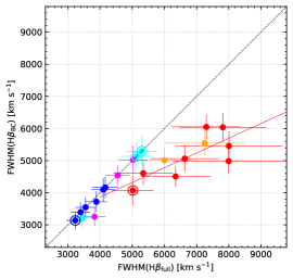
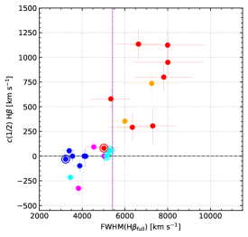
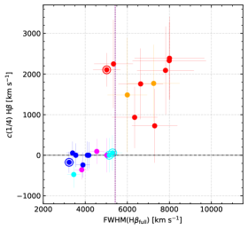
Figure 4: Left panel: FWHM(H$\beta_{\rm BC}$) vs. FWHM of the full H$\beta$ profile. Central panel: velocity centroid at 1/2 intensity $c$(1/2) vs. FWHM(H$\beta_{\rm full}$). Right panel: velocity centroid at 1/4 flux intensity $c$(1/4) vs. FWHM(H$\beta_{\rm full}$). Symbols surrounded by open circles show the radio-loud sources and filled circles represent the radio-quiet from the sample. Red line represent the linear regression performed for Pop. B. Horizontal dashed lines in the central and right panels indicate $c$(1/4) $=0$ and $c$(1/2) $=0$ for H$\beta$, respectively. Purple vertical dashed lines shows the boundary between Pop. A and Pop. B. The many MS spectral type (ST) are represented in different colours: A1 ($\bullet$); A2 ($\bullet$); A3 ($\bullet$); B1 ($\bullet$); and B2 ($\bullet$).

Semi-broad H$\beta$ blueshifts could be mainly associated with the [O III]$\lambda\lambda$4959,5007 SBC. However in some cases an additional BLUE H$\beta$ component is needed (see Table 5). PKS 2126-15 presents a huge BLUE blueshift of $\approx-4700$ km s^-1, associated with a boxy termination of the H$\beta$ blue wing. A second peculiarity of this source is that the H$\beta$ BC is significantly shifted to the blue, down to half maximum, at variance with all other Pop. B sources.

The H$\beta$ NC is weak especially in Pop. A ($\lesssim 0.02$ of the H$\beta$ line flux) although it is observed in all cases save two Pop. A2 sources (SDSSJ132012.33+142037.1 and Q 1410+096). In Pop. B, the narrow component is somewhat stronger but always $\lesssim 0.05$ of the line flux. Given its weakness, the NC is therefore not significantly affecting the flux of any broad component measured in this paper.

Relation between FWHM(H$\beta_{\rm{full}}$) and FWHM(H$\beta_{\rm{BC}}$).

This work confirms previous studies (e.g. Sulentic et al., 2006b; Marziani et al., 2009, and references therein) that showed that the full H$\beta$ profile of Pop. A can be accounted for mostly by the BC, and that a redshifted VBC seems to be absent in Population A but present in Pop. B sources: Table 5 lists centroid and asymmetry index values for Pop. B sources of $1000\lesssim c(\frac{1}{4})\lesssim 2000$ km s^-1 and $\approx 0.2$, respectively. For Pop. A these values are $\lesssim 0$ km s^-1 and 0.

The left plot of Fig. 4 shows the relation between the FWHM of the BC and the FWHM of the full profile of H$\beta$ for the two populations. Pop. A and Pop. B sources follow different trends for the ratio $\xi(\rm H\beta)=$ FWHM(H$\beta_{\rm BC}$)/FWHM(H$\beta_{\rm full}$). For Pop. A quasars, we obtain $\xi(\rm H\beta)=1.00$ for all sources but four (SDSSJ005700.18+143737.7, SDSSJ132012.33+142037.1, SDSSJ161458.33+144836.9, and PKS2000-330, with $\xi(\rm H\beta)\approx 0.9$ due to the presence of a blueshifted component). The $\xi(\rm H\beta)$ ratio for Pop. B is only $\approx$ 0.76, indicating that the Pop. B H$\beta$ full profile is less representative of the BC than the Pop. A sources. Similar results were also shown by Marziani et al. (2013): they obtain $\xi(\rm H\beta)=1.00$ for Pop. A and $\sim 0.78$ for Pop. B quasars. In our sample Pop. B sources usually present a very strong and wide VBC component that accounts for $\approx 0.57$ of the profile, with a mean FWHM of 11240 km s^-1. Meanwhile, as mentioned, the Pop. A sources in general are well represented by only a BC. This also seems to be true for the radio-loud Pop. A sources from the sample.

Clear distinctions between Pop. A and Pop. B are also seen in the center and left panels of Fig. 4, which present the $c$(1/2) and $c$(1/4) vs. FWHM(H$\beta_{\rm{full}}$) relations, respectively. Pop. A sources show in general no shift, within the uncertainties, or a negative value of velocity centroids in the case of the 4 sources with a BLUE component (with average centroid values at 1/2 and 1/4 of -167 and -312 km s^-1, respectively). On the other hand, Pop. B sources always present positive velocities for $c$(1/2) and $c$(1/4), with a mean value of $658$ and $1929$ km s^-1, respectively, as a consequence of a very strong VBC. The VBC individually has a median velocity shift of $\sim 3000$ km s^-1, in a range from $-1500$ to $4000$ km s^-1. These results are in complete agreement with previous results (e.g. Wolf et al., 2020, and references therein).

Table 6: Measurements on the [O III]$\lambda 5007$ full line profile.

	[O III]$\lambda 5007$ full profile						SBC				NC
Source	FWHM	A. I.	Kurtosis	$c$(1/2)	$c$(9/10)		$I/I_{\mathrm{tot}}$	FWHM	Shift		$I/I_{\mathrm{tot}}$	FWHM	Shift
	[km s-1]			[km s-1]	[km s-1]			[km s-1]	[km s-1]			[km s-1]	[km s-1]
(1)	(2)	(3)	(4)	(5)	(6)		(7)	(8)	(9)		(10)	(11)	(12)
Population A
SDSSJ005700.18+143737.7(a)	764::	-0.01::	0.45::	-89::	-88::		0.27::	1214::	-1856::		0.732::	761::	-87::
SDSSJ132012.33+142037.1	2124 $\pm$ 147	-0.54 $\pm$ 0.01	0.23 $\pm$ 0.01	-770 $\pm$ 62	-221 $\pm$ 36		0.64 $\pm$ 0.06	2275 $\pm$ 235	-1429 $\pm$ 115		0.357 $\pm$ 0.114	895 $\pm$ 95	-149 $\pm$ 22
SDSSJ135831.78+050522.8	4320 $\pm$ 297	-0.43 $\pm$ 0.05	0.19 $\pm$ 0.10	-1895 $\pm$ 91	-630 $\pm$ 59		0.90 $\pm$ 0.08	5422 $\pm$ 561	-2080 $\pm$ 100		0.096 $\pm$ 0.031	1000 $\pm$ 106	-534 $\pm$ 80
Q 1410+096	3363 $\pm$ 283	-0.52 $\pm$ 0.01	0.28 $\pm$ 0.01	-1404 $\pm$ 107	-656 $\pm$ 72		0.73 $\pm$ 0.07	5573 $\pm$ 577	-1255 $\pm$ 96		0.267 $\pm$ 0.085	1379 $\pm$ 147	-260 $\pm$ 39
B1422+231	1535 $\pm$ 99	-0.18 $\pm$ 0.01	0.43 $\pm$ 0.01	-217 $\pm$ 26	-88 $\pm$ 47		0.32 $\pm$ 0.03	1128 $\pm$ 117	-850 $\pm$ 102		0.680 $\pm$ 0.218	1117 $\pm$ 119	27 $\pm$ 4
SDSSJ161458.33+144836.9	2616 $\pm$ 160	-0.49 $\pm$ 0.01	0.28 $\pm$ 0.02	-1452 $\pm$ 54	-800 $\pm$ 50		0.75 $\pm$ 0.07	2759 $\pm$ 286	-1875 $\pm$ 70		0.245 $\pm$ 0.078	1006 $\pm$ 107	-667 $\pm$ 100
PKS 1937-101	1046 $\pm$ 79	-0.15 $\pm$ 0.09	0.35 $\pm$ 0.02	-155 $\pm$ 17	-135 $\pm$ 31		0.57 $\pm$ 0.05	2657 $\pm$ 275	-484 $\pm$ 53		0.432 $\pm$ 0.138	832 $\pm$ 88	-120 $\pm$ 18
PKS 2000-330	1314 $\pm$ 89	-0.13 $\pm$ 0.01	0.42 $\pm$ 0.01	-425 $\pm$ 22	-371 $\pm$ 41		0.42 $\pm$ 0.04	1500 $\pm$ 155	-827 $\pm$ 43		0.578 $\pm$ 0.185	1082 $\pm$ 115	-263 $\pm$ 39
SDSSJ210524.49+000407.3	1365::	0.00::	0.45::	201::	202::		1.00::	1361::	203::		0.000	…	…
SDSSJ210831.56-063022.5	3665::	0.00::	0.46::	-1243::	-1242::		1.00::	3679::	-1244::		0.000	…	…
SDSSJ212329.46-005052.9	3656 $\pm$ 247	-0.04 $\pm$ 0.04	0.39 $\pm$ 0.02	-2885 $\pm$ 58	-2584 $\pm$ 119		0.88 $\pm$ 0.08	4719 $\pm$ 488	-2376 $\pm$ 48		0.115::	2043::	174::
SDSSJ235808.54+012507.2	1870 $\pm$ 224	0.00 $\pm$ 0.03	0.46 $\pm$ 0.01	-943 $\pm$ 78	-942 $\pm$ 49		1.00 $\pm$ 0.09	2464 $\pm$ 255	-1053 $\pm$ 87		0.000	…	…
Median	1997 $\pm$ 2045	-0.14 $\pm$ 0.42	0.40 $\pm$ 0.17	-856 $\pm$ 1214	-500 $\pm$ 707		0.68 $\pm$ 0.49	2560 $\pm$ 2032	-1249 $\pm$ 1016		0.312 $\pm$ 0.493	1082 $\pm$ 427	-120 $\pm$ 288
Population B
HE 0001-2340	1029 $\pm$ 145	-0.07 $\pm$ 0.10	0.40 $\pm$ 0.02	-24 $\pm$ 30	-12 $\pm$ 64		0.43 $\pm$ 0.03	2768 $\pm$ 90	-443 $\pm$ 554		0.565 $\pm$ 0.202	894 $\pm$ 65	-1 $\pm$ 10
$[\rm HB89]$ 0029+073	1866 $\pm$ 271	-0.47 $\pm$ 0.01	0.38 $\pm$ 0.01	-922 $\pm$ 97	-562 $\pm$ 114		1.00 $\pm$ 0.06	3431 $\pm$ 168	-397 $\pm$ 42		0.000	…	…
CTQ 408	1497 $\pm$ 190	0.00 $\pm$ 0.01	0.46 $\pm$ 0.01	-524 $\pm$ 37	-524 $\pm$ 97		1.00 $\pm$ 0.09	1500 $\pm$ 401	-524 $\pm$ 37		0.000	…	…
H 0055-2659	1405 $\pm$ 325	-0.47 $\pm$ 0.06	0.25 $\pm$ 0.01	-198 $\pm$ 103	-91 $\pm$ 81		0.50 $\pm$ 0.07	3204 $\pm$ 412	-599 $\pm$ 312		0.496 $\pm$ 0.177	912 $\pm$ 66	69 $\pm$ 10
SDSSJ114358.52+052444.9	2577 $\pm$ 251	0.05 $\pm$ 0.03	0.54 $\pm$ 0.02	-968 $\pm$ 52	-1079 $\pm$ 186		0.78 $\pm$ 0.03	1982 $\pm$ 83	-1295 $\pm$ 70		0.220 $\pm$ 0.078	1304 $\pm$ 94	-1 $\pm$ 10
SDSSJ115954.33+201921.1	1233 $\pm$ 186	-0.20 $\pm$ 0.10	0.37 $\pm$ 0.03	-347 $\pm$ 46	-302 $\pm$ 76		0.55 $\pm$ 0.07	2684 $\pm$ 204	-499 $\pm$ 66		0.448 $\pm$ 0.160	995 $\pm$ 72	-261 $\pm$ 39
SDSSJ120147.90+120630.2	2584 $\pm$ 200	-0.10 $\pm$ 0.01	0.61 $\pm$ 0.01	-594 $\pm$ 49	-504 $\pm$ 126		0.72 $\pm$ 0.05	1879 $\pm$ 196	-978 $\pm$ 81		0.280 $\pm$ 0.100	1129 $\pm$ 82	244 $\pm$ 37
SDSSJ141546.24+112943.4	1193 $\pm$ 204	-0.37 $\pm$ 0.01	0.38 $\pm$ 0.01	-116 $\pm$ 70	55 $\pm$ 75		0.47 $\pm$ 0.04	1499 $\pm$ 111	-415 $\pm$ 250		0.526 $\pm$ 0.188	700 $\pm$ 51	151 $\pm$ 23
SDSSJ153830.55+085517.0	1520 $\pm$ 192	0.00 $\pm$ 0.01	0.46 $\pm$ 0.01	-545 $\pm$ 38	-545 $\pm$ 97		1.00 $\pm$ 0.09	1523 $\pm$ 101	-545 $\pm$ 38		0.000	…	…
PKS 2126-15	1212 $\pm$ 167	-0.22 $\pm$ 0.03	0.41 $\pm$ 0.01	-441 $\pm$ 44	-355 $\pm$ 75		0.30 $\pm$ 0.09	1332 $\pm$ 272	-988 $\pm$ 99		0.702 $\pm$ 0.250	937 $\pm$ 68	-285 $\pm$ 43
Median	1451 $\pm$ 562	-0.15 $\pm$ 0.31	0.40 $\pm$ 0.08	-482 $\pm$ 346	-429 $\pm$ 396		0.52 $\pm$ 0.32	1930 $\pm$ 1241	-534 $\pm$ 426		0.364 $\pm$ 0.463	937 $\pm$ 159	-1 $\pm$ 241

5.2.2 [O III]$\lambda\lambda 4959,5007$

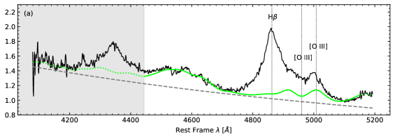
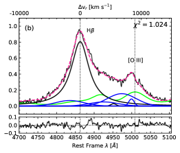
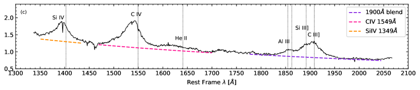
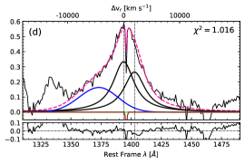
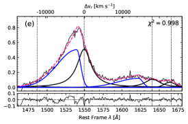
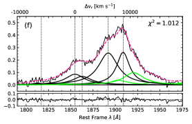
Figure 27: SDSSJ135831.78+050522.8. Same as Figure 23.

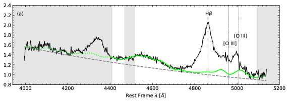
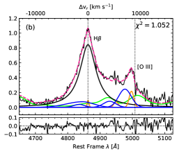
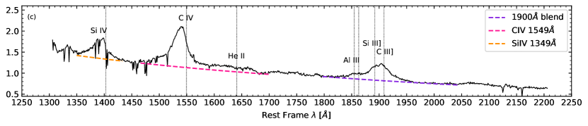
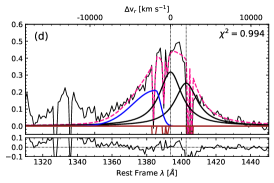
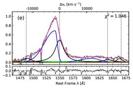
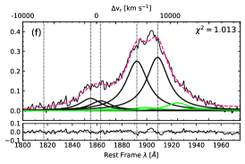
Figure 32: SDSSJ161458.33+144836.9. Same as Figure 23.

High-ionisation lines like [O III]$\lambda\lambda$4959,5007 are seen as one of the main detectors of outflowing gas in radio-quiet sources (Zamanov et al., 2002; Komossa et al., 2008; Zhang et al., 2011; Marziani et al., 2016b). In the case of radio-loud sources, narrow-line outflowing gas has been associated with jets through the blueshifted line components (Capetti et al., 1996; Axon et al., 2000; Bicknell, 2002; Kauffmann et al., 2008; Best & Heckman, 2012; Reynaldi & Feinstein, 2013; Jarvis et al., 2019; Berton & Järvelä, 2021). Outflows are also detected in H$\beta$. Usually, the blueshifted components on the H$\beta$ profile are related to those found for the [O III]$\lambda\lambda$4959,5007 lines (Carniani et al., 2015; Cresci et al., 2015; Brusa et al., 2015; Marziani et al., 2022b). Results obtained for [O iii]$\lambda 5007$ full profile and individual components are reported in Table 6. We present FWHM (Col. 2), asymmetry (Col. 3), kurtosis (Col. 4), and the centroid velocities at 1/2 and 9/10 intensities (Cols. 5 and 6, respectively) for the full profile. Relative intensities, FWHM, and shifts are reported for the [O iii]$\lambda 5007$ blueshifted components (Cols. 7 to 9) and for the narrow components (Cols. 10 to 12) of each quasar. It is difficult to distinguish the relative contribution of the two components in the majority of the cases. One of the main reasons for this is that in many sources the full [O iii]$\lambda 5007$ emission is shifted to the blue, implying a shift of [O iii]$\lambda 5007$ NC with respect to the rest-frame. Some sources like SDSSJ135831.78+050522.8 and SDSSJ161458.33+144836.9 present a NC strongly shifted to the blue, reaching shifts of $\approx-530$ and $-670$ km s^-1 respectively, comparable to the shifts found for the semi-broad component (see e.g. Figs. 27 and 32 in the Appendix A).This is consistent with outflowing gas dominating the [O III]$\lambda$5007 luminosity in luminous quasars (Shen & Ho, 2014; Bischetti et al., 2017; Zakamska et al., 2016).

The remarkable feature of the [O III]$\lambda\lambda$4959,5007 profiles is a very intense and blueshifted SBC, such as the one of SDSSJ135831.78+050522.8 (Fig. 27), which presents a blueshifted SBC that accounts for the full [O III]$\lambda$5007 profile with a FWHM $\approx 5422$ km s^-1 and a shift of $\approx-2080$ km s^-1. In this case, the blueshifted SBC corresponds to 90% of the full profile and can be interpreted as a strong indicative of outflowing gas. SDSSJ135831.78+050522.8, along with Q 1410+096 (Fig. 28 in the Appendix A) which shows a very similar profile, requires a strong and broad [O III]$\lambda$5007 to account for the flux on the red side of H$\beta$. In our high luminosity sample, for 15/22 objects ($\sim$ 70%) the blueshifted SBC accounts for more than 50% of the total intensity of the [O III] profile. In fact, in 6 of these sources, the [O III] consists of exclusively a blueshifted SBC.

Very small blueshifted components are found in low-redshift [O III]$\lambda\lambda$4959,5007 profiles of Pop. B AGN (Zamfir et al., 2008; Sulentic et al., 2004) and even in Population A, shifts at peak above 250 km s^-1 are very rare (the so-called “blue-outliers”; Zamanov et al. 2002). At high-redshift, Pop. B [O III]$\lambda\lambda$4959,5007 profiles do present significant blueshifted SBC components but they still present different properties when compared to Pop. A sources: in our sample, the full profiles of Pop. A present a [O III] FWHM $\approx 2000$ km s^-1 while Pop. B profiles have FWHM $\approx 1450$ km s^-1. The more remarkable difference is seen in the shifts at 9/10 and 1/2 intensities of the full profile ($c$(1/2) $\approx-850$ km s^-1 for Pop. A and $\approx-480$ km s^-1 for Pop. B). However, the A.I. of the two populations are almost the same, indicating that the lines present similar profile shapes. The [O III]$\lambda\lambda$4959,5007 emission of both Pop. A and Pop. B appears to be strongly affected (if not dominated) by outflowing gas.

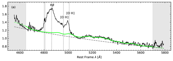
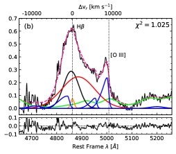
Figure 19: $[\rm HB89]$ 0029+073. Colors and lines as Figure 18.

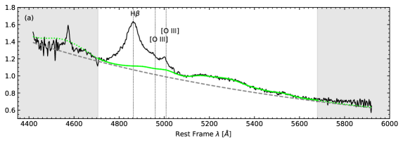
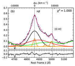
Figure 20: CTQ 0408. Same as Figure 18.

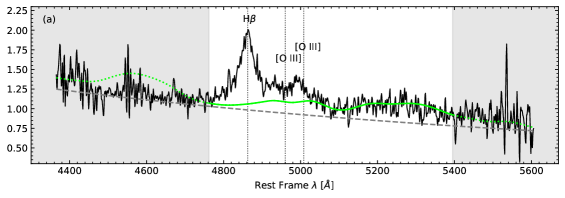
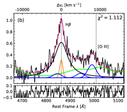
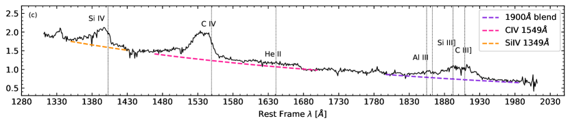
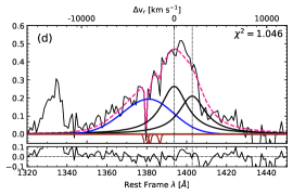
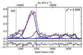
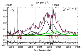
Figure 39: SDSSJ235808.54+012507.2. Same as Figure 23.

An important consequence for redshift estimates is that the [O III]$\lambda\lambda$4959,5007 lines should be avoided when considering high-$z$ quasars. In addition, three Pop. A (SDSSJ210524.49+000407.3, SDSSJ210831.56-063022.5, and SDSSJ235808.54+012507.2) and three Pop. B sources ([HB89] 0029+073, CTQ 0408, and SDSSJ153830.55+085517.0) present [O iii]$\lambda 5007$ full profiles that can be well represented only by the blueshifted component (see the respective spectra in Figs. 39, 19, 20, and 31 in the Appendix A).

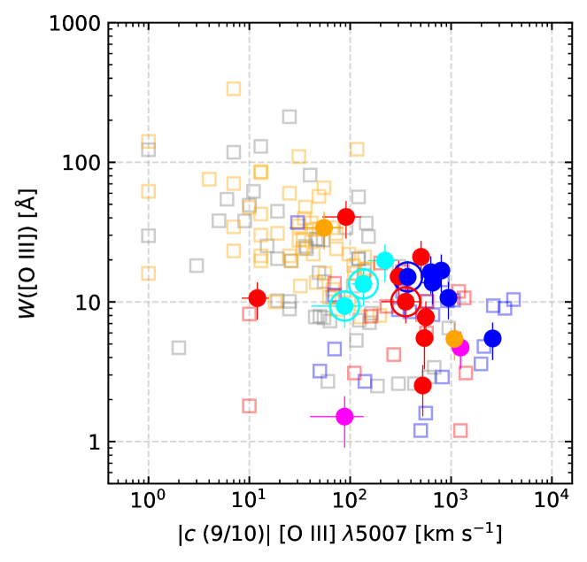
Figure 5: $W$([O III]$\lambda$5007) versus $c$(9/10). Blue and red squares indicate high-redshift Pop. A and Pop. B quasars from M09 while grey and orange open squares represent low-$z$ sources from Marziani et al. (2003), respectively. Color scheme for our sample as in Fig. 4. Error bars refer to 1$\sigma$ level of confidence and were estimated only for our sample.

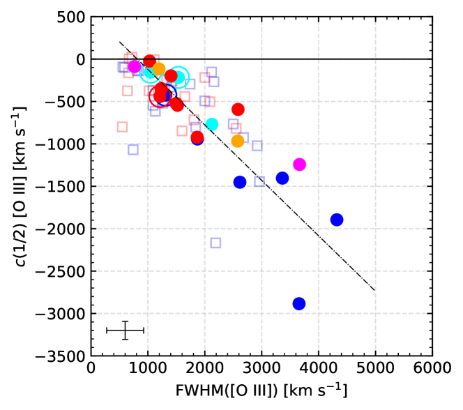
Figure 6: FWHM of the full profile of [O III]$\lambda\lambda$4959,5007 versus centroid at 1/2 flux intensity (c(1/2)) for the [O III]$\lambda\lambda$4959,5007 emission line. Blue and red squares indicate high-redshift sources from M09. Dashed line represents a linear regression. Color scheme as in Fig. 4. Error bars refer to 1$\sigma$ level of confidence and were estimated only for our sample.

Fig. 5 shows the relation between $W$([O III]) and —$c$(9/10)— of [O III]$\lambda$5007. For our sample, the $W$([O III]) ranges from $\approx$ 50Å  for some Pop. B sources to $<1\r{A}$ for xAs, reaching the detection limit. It shares the same location as the high-redshift HE data. No clear difference between the location of Pop. A and Pop. B is confirmed by the median values of equivalent widths, 12Å vs. 10Å for Pop. A and B, respectively (the average $W$ is affected by the two A3 extremely faint sources with $W$([O III]) $\lesssim 1$Å). At low $z$ (and low luminosity), sources have considerably larger $W$ values but lower velocity centroids than the high-$z$ sample. Our sample is located at the low end of the $W$([O III]) distribution of low-$z$ sources as expected for luminous quasars (Shen & Ho, 2014), and in a shift range that at low $z$ is the exclusive domain of the rare, namesake “blue outliers” (Marziani et al., 2016a). Fig. 5 also shows that the radio-loud quasars from our sample are very tightly grouped together with moderate blueshifts for high-$L$ quasars ($\lesssim 500$ km s^-1 at 0.9 fractional intensity).

A comparison between $c$(1/2) and FWHM of the [O III]$\lambda$5007 profiles is shown in Fig. 6. There is a strong correlation between the blueshift of [O III], parameterised by the centroid at 1/2 intensity, and the FWHM. The dashed line in the plot traces the linear regression between both parameters, derived from an unweighted least squares fit:

$$c(1/2)_{\rm[{O\textsc{III}}]}\approx(-0.65\pm 0.08)\ \textrm{FWHM}({\rm[{O\textsc{III}}]})+(530\pm 205),$$ (1)

Table 6 lists this linear relation together with the other that involve also C IV$\lambda$1549. We report the fitted parameters (Cols. 1 and 2), the method used (Col. 3), the linear correlation coefficients (Cols. 4 and 5), the rms (Col. 6), the Pearson $r$ score (Col. 7), and its associated null hypothesis probability value (Col. 8). Equation 1 confirms several previous works (Komossa et al., 2008; Marziani et al., 2016b) and justifies the interpretation of the [O III]$\lambda$5007 profile in terms of a blueshifted semibroad component and of a narrow component (Zhang et al., 2011).

Table 7: Linear relations ($y=a+b*x$) between different emission line properties.

y	x	Method	$a\pm\delta a$	$b\pm\delta b$	RMSE	CC	$\rho$-value
(1)	(2)	(3)	(4)	(5)	(6)	(7)	(8)
$c(1/2)_{\rm{[{O\textsc{iii}}]}}$	$\rm{FWHM}(\rm{[{O\textsc{iii}}]})$	Least squares	$530\pm 205$	$-0.65\pm 0.08$	402	-0.86	$4.1\times 10^{-7}$
$c(1/2)_{\rm{{C\textsc{IV}}}}$	$\rm{FWHM}(\rm{{C\textsc{IV}}})$	Least squares	$2000\pm 737^{(a)}$	$-0.68\pm 0.10^{(a)}$	429	-0.90(a)	$1.1\times 10^{-4}$ (a)
$\log W(\textrm{{C {IV}}})$	$\log|c(1/2)|_{\rm{{C\textsc{IV}}}}$	Bisector	$3.21\pm 0.17^{(a)}$	$-0.58\pm 0.05^{(a)}$	0.28	-0.64(a)	$2.1\times 10^{-12}$ (a)
$\log W(\textrm{{C {IV}}})$	$\log\textrm{FWHM({C {IV}})}$	Bisector	$8.31\pm 0.71^{(a)}$	$-1.84\pm 0.19^{(a)}$	0.31	-0.49(a)	$2.5\times 10^{-7}$ (a)
$c(1/2)_{\rm{{C\textsc{IV}}}}$	$c(1/2)_{\rm{[{O\textsc{III}}]}}$	Orthogonal	$-1239\pm 276$	$1.50\pm 0.31$	1086	0.45	$4\times 10^{-3}$

Table 8: Spectrophotometric measurements on the UV region.

Source	$f_{\lambda,1750}$ (a)	$f$(Si IV+O IV)(b)	W(Si IV+O IV)	$f$(C IV)(b)	$W$(C IV)	$f$(He II)(b)	$W$(He II)	$f$(Al III)(b)	$W$(Al III)	$f$(C III])(b)	$W$(C III])	$f$(Si III])(b)	$W$(Si III])
			[Å]		[Å]		[Å]		[Å]		[Å]		[Å]
(1)	(2)	(3)	(4)	(5)	(6)	(7)	(8)	(9)	(10)	(11)	(12)	(13)	(14)
Population A
SDSSJ005700.18+143737.7(e)	5.9 $\pm$ 0.9	1.29 $\pm$ 0.19	16 $\pm$ 2	1.58 $\pm$ 0.24	22 $\pm$ 3	0.33 $\pm$ 0.05	5 $\pm$ 1	0.41 $\pm$ 0.06	8 $\pm$ 1	0.23 $\pm$ 0.03	5 $\pm$ 1	0.42 $\pm$ 0.06	8 $\pm$ 1
SDSSJ132012.33+142037.1	7.9 $\pm$ 1.2	1.77 $\pm$ 0.27	18 $\pm$ 2	3.66 $\pm$ 0.55	40 $\pm$ 5	0.81 $\pm$ 0.12	10 $\pm$ 1	0.31 $\pm$ 0.05	4 $\pm$ 1	0.57 $\pm$ 0.09	8 $\pm$ 1	0.75 $\pm$ 0.11	11 $\pm$ 1
SDSSJ135831.78+050522.8	13.6 $\pm$ 2.0	3.78 $\pm$ 0.57	20 $\pm$ 2	5.43 $\pm$ 0.81	34 $\pm$ 4	1.31 $\pm$ 0.20	9 $\pm$ 1	0.89 $\pm$ 0.13	7 $\pm$ 1	1.01 $\pm$ 0.15	9 $\pm$ 1	1.52 $\pm$ 0.23	13 $\pm$ 2
Q 1410+096	14.1 $\pm$ 2.1	2.45 $\pm$ 0.37	15 $\pm$ 2	3.50 $\pm$ 0.53	23 $\pm$ 3	1.50 $\pm$ 0.23	10 $\pm$ 1	0.96 $\pm$ 0.14	7 $\pm$ 1	1.17 $\pm$ 0.18	9 $\pm$ 1	1.18 $\pm$ 0.18	9 $\pm$ 1
SDSSJ161458.33+144836.9	15.4 $\pm$ 2.3	2.90 $\pm$ 0.44	14 $\pm$ 2	5.74 $\pm$ 0.86	31 $\pm$ 4	0.94 $\pm$ 0.14	6 $\pm$ 1	0.57 $\pm$ 0.09	4 $\pm$ 1	1.41 $\pm$ 0.21	11 $\pm$ 1	1.32 $\pm$ 0.20	10 $\pm$ 1
PKS 2000-330(c)	-	3.20 $\pm$ 0.48	4 $\pm$ 2	4.50 $\pm$ 0.68	19 $\pm$ 2	-	-	-	-	-	-	-	-
SDSSJ210524.47+000407.3(d)(e)	21.8 $\pm$ 3.3	-	-	1.50 $\pm$ 0.23	6 $\pm$ 1	0.75 $\pm$ 0.11	3 $\pm$ 1	2.19 $\pm$ 0.33	10 $\pm$ 1	0.51 $\pm$ 0.08	2 $\pm$ 1	1.97 $\pm$ 0.30	9 $\pm$ 1
SDSSJ210831.56-063022.5(e)	14.3 $\pm$ 2.1	2.47 $\pm$ 0.37	14 $\pm$ 2	2.25 $\pm$ 0.34	13 $\pm$ 2	0.14 $\pm$ 0.02	1 $\pm$ 1	1.01 $\pm$ 0.15	7 $\pm$ 1	0.31 $\pm$ 0.05	2 $\pm$ 1	0.94 $\pm$ 0.14	7 $\pm$ 1
SDSSJ212329.46-005052.9	23.9 $\pm$ 3.6	3.58 $\pm$ 0.54	9 $\pm$ 1	6.09 $\pm$ 0.91	19 $\pm$ 2	0.85 $\pm$ 0.13	3 $\pm$ 1	1.77 $\pm$ 0.27	9 $\pm$ 1	0.59 $\pm$ 0.09	3 $\pm$ 1	1.89 $\pm$ 0.28	10 $\pm$ 1
SDSSJ235808.54+012507.2	7.5 $\pm$ 1.1	1.52 $\pm$ 0.23	12 $\pm$ 1	2.55 $\pm$ 0.38	25 $\pm$ 3	0.71 $\pm$ 0.11	8 $\pm$ 1	1.91 $\pm$ 0.29	5 $\pm$ 1	0.47 $\pm$ 0.07	8 $\pm$ 1	0.61 $\pm$ 0.09	10 $\pm$ 1
Population B
SDSSJ114358.52+052444.9	20.2 $\pm$ 3.0	2.28 $\pm$ 0.34	8 $\pm$ 1	5.86 $\pm$ 0.88	24 $\pm$ 3	1.42 $\pm$ 0.21	6 $\pm$ 1	0.71 $\pm$ 0.11	4 $\pm$ 1	1.30 $\pm$ 0.20	7 $\pm$ 1	0.98 $\pm$ 0.15	5 $\pm$ 1
SDSSJ115954.33+201921.1	24.3 $\pm$ 3.6	3.64 $\pm$ 0.55	12 $\pm$ 1	5.55 $\pm$ 0.83	20 $\pm$ 2	0.92 $\pm$ 0.14	4 $\pm$ 1	1.14 $\pm$ 0.17	5 $\pm$ 1	1.94 $\pm$ 0.29	9 $\pm$ 1	0.62 $\pm$ 0.09	3 $\pm$ 1
SDSSJ120147.90+120630.2	16.3 $\pm$ 2.4	3.44 $\pm$ 0.52	15 $\pm$ 2	7.57 $\pm$ 1.14	37 $\pm$ 4	1.63 $\pm$ 0.24	9 $\pm$ 1	0.67 $\pm$ 0.10	5 $\pm$ 1	3.00 $\pm$ 0.45	22 $\pm$ 3	1.13 $\pm$ 0.17	8 $\pm$ 1
SDSSJ141546.24+112943.4(d)	16.8 $\pm$ 2.5	-	-	-	-	-	-	1.59 $\pm$ 0.24	7 $\pm$ 1	5.10 $\pm$ 0.77	23 $\pm$ 3	2.83 $\pm$ 0.42	13 $\pm$ 2
SDSSJ153830.55+085517.0(f)	17.4 $\pm$ 2.6	4.92 $\pm$ 0.74	19 $\pm$ 2	5.34 $\pm$ 0.80	24 $\pm$ 3	0.64 $\pm$ 0.10	3 $\pm$ 1	1.91 $\pm$ 0.29	12 $\pm$ 1	0.94 $\pm$ 0.14	6 $\pm$ 1	1.27 $\pm$ 0.19	8 $\pm$ 1

Table 9: Measurements on the 1900 Å blend.

	Al III$\lambda$1860 BLUE				Al III$\lambda$1860 BC				Si III]$\lambda$1892 BLUE				Si III]$\lambda$1892 BC				C III]$\lambda$1909 BC				C III]$\lambda$1909 VBC				C III]$\lambda$1909 NC				Fe III$\lambda$1914
Source	$I/I_{\rm{tot}}$	FWHM	Shift		$I/I_{\rm{tot}}$	FWHM	Shift		$I/I_{\rm{tot}}$	FWHM	Shift		$I/I_{\rm{tot}}$	FWHM	Shift		$I/I_{\rm{tot}}$	FWHM	Shift		$I/I_{\rm{tot}}$	FWHM	Shift		$I/I_{\rm{tot}}$	FWHM	Shift		$I/I_{\rm{tot}}$	FWHM	Shift
		[km s-1]	[km s-1]			[km s-1]	[km s-1]			[km s-1]	[km s-1]			[km s-1]	[km s-1]			[km s-1]	[km s-1]			[km s-1]	[km s-1]			[km s-1]	[km s-1]			[km s-1]	[km s-1]
(1)	(2)	(3)	(4)		(5)	(6)	(7)		(8)	(9)	(10)		(11)	(12)	(13)		(14)	(15)	(16)		(17)	(18)	(19)		(20)	(21)	(22)		(23)	(24)	(25)
Population A
SDSSJ005700.18+143737.7	0.47 $\pm$ 0.04	3268 $\pm$ 396	-1686 $\pm$ 202		0.53 $\pm$ 0.04	2792 $\pm$ 283	0 $\pm$ 10		0.36 $\pm$ 0.07	3268 $\pm$ 392	-1686 $\pm$ -202		0.64 $\pm$ 0.13	2792 $\pm$ 335	-3 $\pm$ 11		1.00 $\pm$ 0.18	2400 $\pm$ 288	0 $\pm$ 10		…	…	…		…	…	…		1.00 $\pm$ 0.12	2792 $\pm$ 335	1494 $\pm$ 179
SDSSJ132012.33+142037.1	0.27 $\pm$ 0.02	1731 $\pm$ 210	-967 $\pm$ 116		0.72 $\pm$ 0.06	2029 $\pm$ 206	0 $\pm$ 10		0.00	…	…		0.08 $\pm$ 0.02	3030 $\pm$ 364	0 $\pm$ 10		0.92 $\pm$ 0.17	3030 $\pm$ 364	0 $\pm$ 10		…	…	…		…	…	…		1.00 $\pm$ 0.12	3030 $\pm$ 364	1876 $\pm$ 225
SDSSJ135831.78+050522.8	0.00	…	…		1.00 $\pm$ 0.08	4225 $\pm$ 428	0 $\pm$ 10		0.00	…	…		1.00 $\pm$ 0.21	4225 $\pm$ 507	0 $\pm$ 10		1.00 $\pm$ 0.18	2720 $\pm$ 326	0 $\pm$ 10		…	…	…		…	…	…		1.00 $\pm$ 0.12	4231 $\pm$ 508	1033 $\pm$ 124
Q 1410+096	0.00	…	…		1.00 $\pm$ 0.08	2604 $\pm$ 264	279 $\pm$ 33		0.00	…	…		1.00 $\pm$ 0.21	2604 $\pm$ 312	279 $\pm$ 33		1.00 $\pm$ 0.18	2604 $\pm$ 312	278 $\pm$ 58		…	…	…		…	…	…		1.00 $\pm$ 0.12	1607 $\pm$ 193	1253 $\pm$ 150
SDSSJ161458.33+144836.9	0.00	…	…		1.00 $\pm$ 0.08	3374 $\pm$ 342	0 $\pm$ 10		0.00	…	…		1.00 $\pm$ 0.21	3374 $\pm$ 405	0 $\pm$ 10		1.00 $\pm$ 0.18	3319 $\pm$ 398	0 $\pm$ 10		…	…	…		…	…	…		0.00	…	…
SDSSJ210524.49+000407.3	0.61 $\pm$ 0.05	4365 $\pm$ 529	-2003 $\pm$ 240		0.39 $\pm$ 0.03	3672 $\pm$ 372	0 $\pm$ 10		0.23 $\pm$ 0.04	3415 $\pm$ 410	-2002 $\pm$ -240		0.77 $\pm$ 0.16	4169 $\pm$ 500	0 $\pm$ 10		1.00 $\pm$ 0.18	2577 $\pm$ 309	0 $\pm$ 10		…	…	…		…	…	…		1.00 $\pm$ 0.12	3672 $\pm$ 441	771 $\pm$ 93
SDSSJ210831.56-063022.5	0.36 $\pm$ 0.03	3181 $\pm$ 386	-1951 $\pm$ 234		0.64 $\pm$ 0.05	4173 $\pm$ 423	0 $\pm$ 10		0.21 $\pm$ 0.04	3187 $\pm$ 382	-1951 $\pm$ -234		0.79 $\pm$ 0.17	4173 $\pm$ 501	0 $\pm$ 10		1.00 $\pm$ 0.18	3156 $\pm$ 379	0 $\pm$ 10		…	…	…		…	…	…		1.00 $\pm$ 0.12	2177 $\pm$ 261	2102 $\pm$ 252
SDSSJ212329.46-005052.9	0.00	…	…		1.00 $\pm$ 0.08	5122 $\pm$ 519	0 $\pm$ 10		0.00	…	…		1.00 $\pm$ 0.21	5122 $\pm$ 615	0 $\pm$ 10		1.00 $\pm$ 0.18	3125 $\pm$ 375	0 $\pm$ 10		…	…	…		…	…	…		0.00	…	…
SDSSJ235808.54+012507.2	0.00	…	…		1.00 $\pm$ 0.08	3243 $\pm$ 329	0 $\pm$ 10		0.00	…	…		1.00 $\pm$ 0.21	3243 $\pm$ 389	0 $\pm$ 10		1.00 $\pm$ 0.18	3243 $\pm$ 389	0 $\pm$ 10		…	…	…		…	…	…		1.00 $\pm$ 0.12	3204 $\pm$ 384	111 $\pm$ 13
Median	0.00 $\pm$ 0.36	3224 $\pm$ 723	-1818 $\pm$ 457		1.00 $\pm$ 0.36	3374 $\pm$ 1381	…		0.23 $\pm$ 0.07	3268 $\pm$ 114	-1951 $\pm$ 158		…	3374 $\pm$ 1381	…		…	2760 $\pm$ 552	…		…	…	…		…	…	…		…	2298 $\pm$ 1224	1143 $\pm$ 597
Population B
SDSSJ114358.52+052444.9	0.00	…	…		1.00 $\pm$ 0.08	3967 $\pm$ 402	0 $\pm$ 10		0.00	…	…		1.00 $\pm$ 0.18	3967 $\pm$ 476	-3 $\pm$ 11		0.50 $\pm$ 0.10	3967 $\pm$ 476	0 $\pm$ 10		0.50 $\pm$ 0.05	7038 $\pm$ 1253	2842 $\pm$ 369		0.02 $\pm$ 0.01	1000 $\pm$ 178	0 $\pm$ 10		0.00	…	…
SDSSJ115954.33+201921.1	0.00	…	…		1.00 $\pm$ 0.08	4999 $\pm$ 506	0 $\pm$ 10		0.00	…	…		1.00 $\pm$ 0.18	4999 $\pm$ 600	0 $\pm$ 10		0.64 $\pm$ 0.13	4999 $\pm$ 600	0 $\pm$ 10		0.36 $\pm$ 0.03	6563 $\pm$ 1168	1998 $\pm$ 260		0.01 $\pm$ 0.01	733 $\pm$ 130	0 $\pm$ 10		0.00	…	…
SDSSJ120147.90+120630.2	0.00	…	…		1.00 $\pm$ 0.08	3999 $\pm$ 405	0 $\pm$ 10		0.00	…	…		1.00 $\pm$ 0.18	3999 $\pm$ 480	0 $\pm$ 10		0.70 $\pm$ 0.14	3999 $\pm$ 480	0 $\pm$ 10		0.30 $\pm$ 0.03	7046 $\pm$ 1254	2207 $\pm$ 287		0.01 $\pm$ 0.01	999 $\pm$ 178	0 $\pm$ 10		0.00	…	…
SDSSJ141546.24+112943.4	0.00	…	…		1.00 $\pm$ 0.08	5105 $\pm$ 517	0 $\pm$ 10		0.00	…	…		1.00 $\pm$ 0.18	5105 $\pm$ 613	0 $\pm$ 10		0.64 $\pm$ 0.13	4101 $\pm$ 492	0 $\pm$ 10		0.36 $\pm$ 0.03	7365 $\pm$ 1311	3134 $\pm$ 407		0.10 $\pm$ 0.01	1062 $\pm$ 189	0 $\pm$ 10		0.00	…	…
SDSSJ153830.55+085517.0(a)	0.00	…	…		1.00 $\pm$ 0.08	3085 $\pm$ 313	0 $\pm$ 10		0.00	…	…		1.00 $\pm$ 0.18	3085 $\pm$ 370	0 $\pm$ 10		1.00 $\pm$ 0.20	3104 $\pm$ 372	28 $\pm$ 16		…	…	…		0.00	…	…		1.00 $\pm$ 0.12	3141 $\pm$ 377	783 $\pm$ 94
Median	…	…	…		…	3999 $\pm$ 1032	…		…	…	…		…	3999 $\pm$ 1032	…		0.64 $\pm$ 0.06	3999 $\pm$ 134	…		0.36 $\pm$ 0.05	7042 $\pm$ 206	2524 $\pm$ 760		…	999 $\pm$ 83	…		…	…	…

5.3 UV

The fits for the UV emission lines are shown in Appendix A together with the full UV spectra of the 15 available sources (10 Pop. A and 5 Pop. B). Spectrophotometric measurements in the UV region are reported in Table 8 and concern the 1900 Å blend, C iv$\lambda 1549$+He II$\lambda 1640$, as well as flux intensity and equivalent width of Si IV+O IV (Cols. 3-4), C IV (Cols. 5-6), He II (Cols. 7-8), Al III (Cols. 9-10), C III] (Cols. 11-12), and Si III (Cols 13-14).

5.3.1 1900 Å blend

Table 9 presents the measurements resulting from the specfit analysis of the 1900 Å blend. Intensities, FWHM, and shifts are shown for the emission line profiles and their components, whenever the profile presents more than just one component. Cols. 2 to 4 list relative intensity, FWHM and shift of the blueshifted component of Al III$\lambda 1860$; Cols. 5 to 7 show the broad component of Al III$\lambda 1860$; Cols. 8 to 10 for Si III]$\lambda$1892 BLUE; Cols. 11 to 13 for Si III]$\lambda$1892 BC; Cols. 14 to 16, the BC of C III]$\lambda$1909; Cols. 17 to 19, the VBC of C III]$\lambda$1909; Cols. 20 to 22, the NC of C III]$\lambda$1909; and, finally, Cols. 23 to 25 for a Fe III]$\lambda$1914 emission line component.

The Al III$\lambda 1860$ contribution can be well fitted assuming only a BC for all Pop. A sources but four: SDSSJ005700.18+143737.7, SDSSJ210524.49+000407.3, SDSSJ210831.56-063022.5, and SDSSJ132012.33+142037.1. These same three sources are the ones that are located in the A3 region of the quasar MS. In these cases, we need to add a BLUE component with $3000\leq$ FWHM $\leq 4500$ km s^-1 in the Al III$\lambda$1860 doublet and in the Si III]$\lambda$1892 emission line profile. We have imposed the same FWHM for both components.

The Pop. A C III]$\lambda$1909 profile can be well reproduced by a strong BC at rest-frame in combination with a component that accounts for the Fe III$\lambda$1914 contributions in its red wing. The motivation to include the Fe III$\lambda$1914 line resides in the selective enhancement due to Lyman $\alpha$ fluorescence that is well-known to affect the UV Fe II emission and Fe III emission as well (Sigut & Pradhan, 1998; Sigut et al., 2004). Of the Fe II features the UV multiplet 191 at $\lambda$1785 is known to be enhanced by Ly$\alpha$ fluorescence: a strong Fe II UV multiplet 191 may suggest a strong Fe III$\lambda$1914 line. There is an overall consistency between the presence of the Fe III$\lambda$1914 line and the detection of the Fe II feature (8 out of 10 Pop. A sources with UV suitable data have both). However, the relative contribution of the C III]$\lambda$1909 and Fe III$\lambda$1914 remains difficult to ascertain because the two lines are severely blended together and some Fe III$\lambda$1914 emission is already included in the Fe III template.

For Pop. B sources, Al III$\lambda$1860 and Si III]$\lambda$1892 are well represented by only one component and in the five cases these emission lines share the same FWHM and are centred at the respective rest-frame wavelength. However, the C III]$\lambda$1909 VBC is systematically less broad than the H$\beta$ VBC: average FWHM is $\approx 7000$ km s^-1 for C III] versus $\approx 12000$ km s^-1for H$\beta$.

Table 10: Measurements on the C IV$\lambda 1549$+He II$\lambda 1640$ full line profiles and specfit analysis.

								C IV$\lambda 1549$												He II$\lambda 1640$
	C IV$\lambda 1549$ full profile								BLUE				BC				VBC				BLUE				BC				VBC
Source	FWHM	A. I.	Kurt.	c($\frac{1}{4}$)	c($\frac{1}{2}$)	c($\frac{3}{4}$)	c($\frac{9}{10}$)		$I/I_{\mathrm{tot}}$	FWHM	Shift		$I/I_{\mathrm{tot}}$	FWHM	Shift		$I/I_{\mathrm{tot}}$	FWHM	Shift		$I/I_{\mathrm{tot}}$	FWHM	Shift		$I/I_{\mathrm{tot}}$	FWHM	Shift		$I/I_{\mathrm{tot}}$	FWHM	Shift
	[km s-1]			[km s-1]	[km s-1]	[km s-1]	[km s-1]			[km s-1]	[km s-1]			[km s-1]	[km s-1]			[km s-1]	[km s-1]			[km s-1]	[km s-1]			[km s-1]	[km s-1]			[km s-1]	[km s-1]
(1)	(2)	(3)	(4)	(5)	(6)	(7)	(8)		(9)	(10)	(11)		(12)	(13)	(14)		(15)	(16)	(17)		(18)	(19)	(20)		(21)	(22)	(23)		(24)	(25)	(26)
Population A
SDSSJ005700.18+143737.7	8648 $\pm$ 562	-0.38 $\pm$ 0.01	0.40 $\pm$ 0.01	-4951 $\pm$ 334	-3994 $\pm$ 181	-3272 $\pm$ 272	-2604 $\pm$ 326		0.81 $\pm$ 0.05	13187 $\pm$ 1846	-2318 $\pm$ 278		0.19 $\pm$ 0.05	2808 $\pm$ 298	0 $\pm$ 10		…	…	…		0.67 $\pm$ 0.04	13187 $\pm$ 1846	-4249 $\pm$ 510		0.33 $\pm$ 0.02	2808 $\pm$ 298	0 $\pm$ 10		…	…	…
SDSSJ132012.33+142037.1	5549 $\pm$ 399	-0.36 $\pm$ 0.01	0.37 $\pm$ 0.01	-2956 $\pm$ 263	-2407 $\pm$ 124	-1830 $\pm$ 177	-1419 $\pm$ 190		0.72 $\pm$ 0.04	8739 $\pm$ 1223	-1446 $\pm$ 174		0.28 $\pm$ 0.03	3278 $\pm$ 348	0 $\pm$ 10		…	…	…		0.60 $\pm$ 0.04	9837 $\pm$ 1377	-3388 $\pm$ 407		0.40 $\pm$ 0.02	3278 $\pm$ 348	0 $\pm$ 10		…	…	…
SDSSJ135831.78+050522.8	7365 $\pm$ 655	-0.27 $\pm$ 0.03	0.30 $\pm$ 0.01	-3188 $\pm$ 416	-2460 $\pm$ 190	-1808 $\pm$ 256	-1556 $\pm$ 187		0.52 $\pm$ 0.03	11983 $\pm$ 1678	-1909 $\pm$ 229		0.48 $\pm$ 0.02	4404 $\pm$ 468	0 $\pm$ 10		…	…	…		0.55 $\pm$ 0.03	11983 $\pm$ 1678	-3386 $\pm$ 406		0.45 $\pm$ 0.03	4404 $\pm$ 468	0 $\pm$ 10		…	…	…
Q 1410+096	6311 $\pm$ 552	-0.18 $\pm$ 0.05	0.33 $\pm$ 0.01	-2604 $\pm$ 374	-1746 $\pm$ 179	-1052 $\pm$ 172	-1691 $\pm$ 90		0.41 $\pm$ 0.03	10881 $\pm$ 1523	-1526 $\pm$ 183		0.59 $\pm$ 0.01	3293 $\pm$ 350	0 $\pm$ 10		…	…	…		0.53 $\pm$ 0.03	9369 $\pm$ 1312	-7880 $\pm$ 946		0.47 $\pm$ 0.03	3292 $\pm$ 350	0 $\pm$ 10		…	…	…
SDSSJ161458.33+144836.9	5790 $\pm$ 554	-0.27 $\pm$ 0.03	0.30 $\pm$ 0.02	-2779 $\pm$ 327	-2394 $\pm$ 139	-1894 $\pm$ 190	-1519 $\pm$ 168		0.59 $\pm$ 0.04	9333 $\pm$ 1307	-1609 $\pm$ 193		0.41 $\pm$ 0.01	3816 $\pm$ 406	0 $\pm$ 10		…	…	…		0.66 $\pm$ 0.04	9556 $\pm$ 1338	-5483 $\pm$ 658		0.34 $\pm$ 0.02	3816 $\pm$ 406	0 $\pm$ 10		…	…	…
PKS 2000-330	4950 $\pm$ 346	-0.33 $\pm$ 0.01	0.39 $\pm$ 0.01	-2373 $\pm$ 226	-1923 $\pm$ 104	-1465 $\pm$ 154	-1155 $\pm$ 169		0.70 $\pm$ 0.04	7340 $\pm$ 1028	-1300 $\pm$ 156		0.30 $\pm$ 0.02	3142 $\pm$ 334	0 $\pm$ 10		…	…	…		…	…	…		…	…	…		…	…	…
SDSSJ210524.49+000407.3	8443 $\pm$ 592	-0.15 $\pm$ 0.01	0.43 $\pm$ 0.01	-5060 $\pm$ 297	-4695 $\pm$ 134	-4452 $\pm$ 228	-4175 $\pm$ 279		0.89 $\pm$ 0.05	10418 $\pm$ 1459	-3926 $\pm$ 471		0.11 $\pm$ 0.02	3504 $\pm$ 372	-82 $\pm$ 20		…	…	…		0.55 $\pm$ 0.03	10418 $\pm$ 1459	-8749 $\pm$ 1050		0.45 $\pm$ 0.03	3504 $\pm$ 372	-81 $\pm$ 20		…	…	…
SDSSJ210831.56-063022.5	9389 $\pm$ 619	-0.30 $\pm$ 0.01	0.42 $\pm$ 0.01	-5744 $\pm$ 365	-4982 $\pm$ 177	-4284 $\pm$ 264	-3709 $\pm$ 334		0.87 $\pm$ 0.05	13618 $\pm$ 1907	-3250 $\pm$ 390		0.13 $\pm$ 0.01	4340 $\pm$ 461	0 $\pm$ 10		…	…	…		0.70 $\pm$ 0.04	13618 $\pm$ 1907	-3250 $\pm$ 390		0.30 $\pm$ 0.02	4340 $\pm$ 461	0 $\pm$ 10		…	…	…
SDSSJ212329.46-005052.9	7978 $\pm$ 524	-0.21 $\pm$ 0.01	0.42 $\pm$ 0.01	-3752 $\pm$ 332	-3311 $\pm$ 139	-2876 $\pm$ 231	-2551 $\pm$ 277		0.72 $\pm$ 0.04	10217 $\pm$ 1430	-2694 $\pm$ 323		0.28 $\pm$ 0.01	5457 $\pm$ 580	0 $\pm$ 10		…	…	…		0.63 $\pm$ 0.04	10217 $\pm$ 1430	-4233 $\pm$ 508		0.37 $\pm$ 0.02	5457 $\pm$ 580	0 $\pm$ 10		…	…	…
SDSSJ235808.54+012507.2	6504 $\pm$ 398	-0.25 $\pm$ 0.01	0.44 $\pm$ 0.01	-3197 $\pm$ 245	-2727 $\pm$ 114	-2312 $\pm$ 186	-2029 $\pm$ 235		0.80 $\pm$ 0.05	8302 $\pm$ 1162	-2163 $\pm$ 260		0.20 $\pm$ 0.01	3468 $\pm$ 369	0 $\pm$ 10		…	…	…		0.49 $\pm$ 0.03	9231 $\pm$ 1292	-5323 $\pm$ 639		0.51 $\pm$ 0.03	3468 $\pm$ 369	0 $\pm$ 10		…	…	…
Median	6934 $\pm$ 2406	-0.27 $\pm$ 0.10	0.39 $\pm$ 0.08	-3192 $\pm$ 1828	-2593 $\pm$ 1426	-2103 $\pm$ 1359	-1860 $\pm$ 1062		0.72 $\pm$ 0.19	10317 $\pm$ 2820	-2036 $\pm$ 1053		0.28 $\pm$ 0.19	3486 $\pm$ 927	…		…	…	…		0.60 $\pm$ 0.11	10217 $\pm$ 2427	-4249 $\pm$ 2095		0.4 $\pm$ 0.11	3504 $\pm$ 1048	…		…	…	…
Population B
SDSSJ114358.52+052444.9	7078 $\pm$ 766	-0.30 $\pm$ 0.05	0.27 $\pm$ 0.01	-3049 $\pm$ 511	-2059 $\pm$ 230	-1375 $\pm$ 204	-1147 $\pm$ 185		0.60 $\pm$ 0.06	14345 $\pm$ 1037	-1497 $\pm$ 180		0.24 $\pm$ 0.04	5055 $\pm$ 365	0 $\pm$ 10		0.16 $\pm$ 0.02	11848 $\pm$ 2109	3822 $\pm$ 515		0.57 $\pm$ 0.06	14345 $\pm$ 1037	-3216 $\pm$ 433		0.17 $\pm$ 0.02	5055 $\pm$ 365	0 $\pm$ 10		0.26 $\pm$ 0.03	11848 $\pm$ 2109	2540 $\pm$ 342
SDSSJ115954.33+201921.1	5741 $\pm$ 585	-0.08 $\pm$ 0.05	0.29 $\pm$ 0.01	-1671 $\pm$ 444	-1851 $\pm$ 122	-1516 $\pm$ 166	-1253 $\pm$ 174		0.54 $\pm$ 0.05	9933 $\pm$ 718	-1307 $\pm$ 157		0.32 $\pm$ 0.05	5716 $\pm$ 413	0 $\pm$ 10		0.14 $\pm$ 0.01	8458 $\pm$ 1506	4397 $\pm$ 592		0.36 $\pm$ 0.04	9933 $\pm$ 718	-1307 $\pm$ 176		0.07 $\pm$ 0.01	5716 $\pm$ 413	0 $\pm$ 10		0.58 $\pm$ 0.06	8458 $\pm$ 1506	4397 $\pm$ 592
SDSSJ120147.90+120630.2	4995 $\pm$ 475	-0.08 $\pm$ 0.04	0.32 $\pm$ 0.01	-1354 $\pm$ 284	-1133 $\pm$ 104	-1061 $\pm$ 148	-1015 $\pm$ 132		0.50 $\pm$ 0.05	7464 $\pm$ 540	-1454 $\pm$ 174		0.35 $\pm$ 0.05	3945 $\pm$ 285	0 $\pm$ 10		0.15 $\pm$ 0.01	6710 $\pm$ 1194	1508 $\pm$ 203		0.44 $\pm$ 0.04	7464 $\pm$ 540	-4676 $\pm$ 630		0.09 $\pm$ 0.01	3945 $\pm$ 285	0 $\pm$ 10		0.47 $\pm$ 0.05	6710 $\pm$ 1194	1508 $\pm$ 203
SDSSJ153830.55+085517.0	5819 $\pm$ 448	-0.41 $\pm$ 0.02	0.35 $\pm$ 0.02	-2841 $\pm$ 303	-2108 $\pm$ 147	-1381 $\pm$ 187	-961 $\pm$ 185		0.68 $\pm$ 0.07	10024 $\pm$ 725	-992 $\pm$ 119		0.32 $\pm$ 0.05	4313 $\pm$ 312	0 $\pm$ 10		…	…	…		0.48 $\pm$ 0.05	10024 $\pm$ 725	-992 $\pm$ 134		0.52 $\pm$ 0.08	4313 $\pm$ 312	0 $\pm$ 10		…	…	…
Median	5780 $\pm$ 1474	-0.17 $\pm$ 0.21	0.30 $\pm$ 0.06	-2256 $\pm$ 1563	-1955 $\pm$ 783	-1378 $\pm$ 342	-1081 $\pm$ 252		0.57 $\pm$ 0.15	9978 $\pm$ 2162	-1380 $\pm$ 415		0.30 $\pm$ 0.07	4129 $\pm$ 1268	…		0.15 $\pm$ 0.01	8458 $\pm$ 2569	3822 $\pm$ 1444		0.46 $\pm$ 0.16	9978 $\pm$ 2087	-2261 $\pm$ 2920		0.14 $\pm$ 0.24	4129 $\pm$ 1255	…		0.47 $\pm$ 0.16	8458 $\pm$ 2569	2540 $\pm$ 1444

5.3.2 C IV$\lambda 1549$+He II$\lambda 1640$

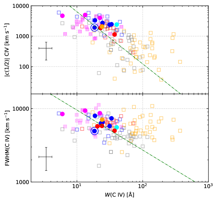
Figure 7: Top: Relation between centroid velocity at 1/2 intensity ($c$(1/2)) and rest-frame equivalent width of C IV$\lambda$1549. Bottom: FWHM of C IV$\lambda$1549 versus $W$(C IV). Colour scheme for our sample as in Fig. 4. Filled magenta squares indicate data from Martínez-Aldama et al. (2018). Blue and red open squares represent Pop. A and Pop. B HE sources from S17. Low-$z$ FOS data from S07 are represented by grey (Pop. A) and orange (Pop. B) squares. Green point-dashed lines indicate the linear regression obtained through the bisector method including only the Pop. A sources from the four samples. Error bars refer to 1$\sigma$ level of confidence and were estimated only for our sample.

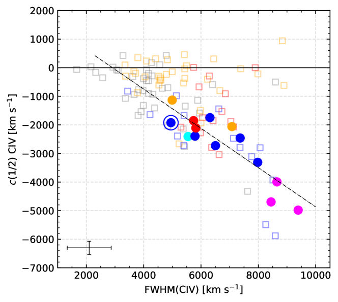
Figure 8: Centroid velocity at 1/2 flux intensity, $c$(1/2), for the C IV$\lambda$1549 emission line versus FWHM of the full profile of C IV. Filled circles represent our sample and the colour scheme is the same as in Fig. 4. Blue and red open squares are high-redshift sources from S17. Low-$z$ Pop. A and Pop. B are represented by grey and orange open squares, respectively. Dashed line represents the least squares linear regression presented in Eq. 2, including only Pop. A sources. Error bars refer to 1$\sigma$ level of confidence for our sample.

Measurements on the C IV$\lambda 1549$+He II$\lambda 1640$ blend are reported in Table 10. As for H$\beta$, we list FWHM (Col. 2), A.I. (Col. 3), kurtosis (Col. 4), and centroids $c$(1/4), $c$(1/2), $c$(3/4) and $c$(9/10) in Cols. 5 to 8 for the C IV$\lambda 1549$ full line profile. Information on individual components is also given for both C IV$\lambda 1549$ and He II$\lambda 1640$. Cols. 9 to 11 give the relative intensity $I/I_{\mathrm{tot}}$, FWHM, and shift for C IV$\lambda 1549$ BLUE; Cols. 12 to 14 for C IV$\lambda 1549$ BC; Cols. 15 to 17 for C IV$\lambda 1549$ VBC; Cols. 18 to 20 for He II$\lambda 1640$ BLUE; Cols. 21 to 23 for He II$\lambda 1640$ BC; and Cols. 24 to 26 for He II$\lambda 1640$ VBC.

We have ten out of 12 Pop. A sources and four out of ten Pop. B quasars with C IV covered for analysis. The fits are remarkably good and allow for the “plateau” found as an extension of the red wing of C IV$\lambda$1549 close to 1575 Å, which can usually be well reproduced by fitting C IV$\lambda 1549$ and He II$\lambda 1640$ with the same FWHM for blueshifted, broad, and very broad components (Fine et al., 2010; Marziani et al., 2010). In general, Pop. A objects present a larger FWHM of the full profile, always $\geq$ 4900 km s^-1, with respect to Pop. B. Pop. A are also those that in general present higher asymmetries and shifts towards the blue. Apart from SDSSJ212329.46-005052.9, all Pop. A sources present a FWHM(C IV_BC) $\leq 4500$ km s^-1. The Pop. A3 SDSSJ210831.56-063022.5 is the source with the strongest blueshift, reaching $c$(1/2) $\approx-4980$ km s^-1 and with similar values of fractional intensities along the profile (as can be seen in the top plot of Fig. 7).

In the case of Pop. B sources, we have found that the VBC accounts for only $\sim 15$% of the full profile. The widest VBC FWHM is seen in SDSSJ114358.52+052444.9, which reaches 11848 km s^-1 with a shift of 3822 km s^-1. This same source is the one that also presents the broadest FWHM of the BLUE (14345 km s^-1) and larger shift ($-1497$ km s^-1). In all Pop. B cases, the BLUE component accounts for at least 50% of the C IV$\lambda$1549 full profile, but still a fraction that is lower than in Pop. A ($\sim$ 70 %). Correspondingly, the Pop. A C IV$\lambda$1549 profiles in general present higher blueshifts and asymmetry indexes than the ones measured in Pop. B.

The top and bottom panels from Fig. 7 show the relation between the rest-frame equivalent widths of C IV$\lambda$1549 and the centroid velocities at 1/2 peak intensity ($c$(1/2)) and FWHM respectively). We also include in the figure the bright, high-$z$ xA sample of Martínez-Aldama et al. (2018) as well as the high-$z$ data from S17 and the FOS low-$z$ data from S07. Our data are in good agreement with the ones of Martínez-Aldama et al. (2018) and S17. Our sample together with the high-$L$ comparison samples, presents smaller values of C IV$\lambda$1549 equivalent width when compared with the FOS data. Additionally, the high-$z$, high-$L$ sources are those that present the most blueshifted C IV$\lambda$1549 profiles among all quasars (Shen et al., 2011; Rankine et al., 2020; Vietri et al., 2018, 2020). The Pearson correlation coefficient between $W$ and $c$(1/2) of C IV$\lambda$1549 for the Pop. A sources is -0.64 (with $\rho=2.1\times 10^{-12}$) and their relation is given in Table 6. There is also a correlation between $W$ and FWHM C IV$\lambda$1549 with $r\approx-0.49$, if we restrict the samples to only Pop. A objects (Table 6).

Fig. 8 presents the strong correlation between FWHM and $c$(1/2) of the C IV line, with a Pearson $r\approx$ -0.90 for high-$z$ Pop. A sources:

$$c(1/2)_{\rm{C\textsc{IV}}}=(-0.68\pm 0.10)\textrm{FWHM}({\rm{{C\textsc{IV}}}})+(2000\pm 737)$$ (2)

This relation is in good agreement with previous results (e.g. Coatman et al., 2016; Marziani et al., 2016a; Sulentic et al., 2017; Sun et al., 2018; Vietri et al., 2018, and references therein). As the blueshift of C IV increases, FWHM(C IV) is likely to increase as well. Both C IV FWHM and blueshift parameterised by $c$(1/2) show a clear increase from spectral types A1 to A3, the latter being those with the highest blueshifts (median value $\approx$ $-4500$ km s^-1) and the widest FWHM (median $\approx$ 9000 km s^-1).

In the case of C IV$\lambda$1549 in Pop. B sources, the shifts at 1/2 flux intensities are also displaced towards blue wavelengths with average value of $c$(1/2) $=-1681$ km s^-1 and mean FWHM $\approx 5940$ km s^-1, somewhat smaller than for Pop. A. However, the $c$(1/2) values for the Pop. B sources from our sample are still higher than the majority of the low-luminosity and low-redshift quasars, which usually present a $c$(1/2) $\leq 200$ km s^-1. Low-luminosity Pop. B spectra show a sort of dichotomy in the C IV$\lambda$1549 shift distribution: a fraction of sources remains unshifted or with modest shifts to the blue (the orange and grey “cloud” of points in Fig. 8). The FOS low-luminosity and low-redshift sources tend to present smaller $c$(1/2) in the C IV$\lambda$1549 emission line when compared with our data. This indicates that the C IV$\lambda$1549 blueshifted components seen in higher-luminosity sources are more prominent than the ones observed in quasars of lower luminosities.

Table 11: Measurements on the full profiles of Si IV$\lambda 1397$+O IV]$\lambda 1402$.

Source	FWHM	A.I.	Kurtosis	$c$(1/2)	$c$(9/10)
	[km s-1]			[km s-1]	[km s-1]
(1)	(2)	(3)	(4)	(5)	(6)
Population A
SDSSJ005700.18+143737.7	8659 $\pm$ 1202	-0.34 $\pm$ 0.02	0.36 $\pm$ 0.03	-2110 $\pm$ 377	-858 $\pm$ 443
SDSSJ132012.33+142037.1	5128 $\pm$ 859	-0.26 $\pm$ 0.05	0.34 $\pm$ 0.01	-376 $\pm$ 249	131 $\pm$ 293
SDSSJ135831.78+050522.8	7438 $\pm$ 1658	-0.27 $\pm$ 0.07	0.31 $\pm$ 0.01	-150 $\pm$ 534	499 $\pm$ 395
Q 1410+096	5430 $\pm$ 790	0.00 $\pm$ 0.09	0.40 $\pm$ 0.01	750 $\pm$ 157	666 $\pm$ 335
SDSSJ161458.33+144836.9	7370 $\pm$ 860	-0.26 $\pm$ 0.06	0.48 $\pm$ 0.01	-392 $\pm$ 227	680 $\pm$ 844
PKS 2000-330	3494 $\pm$ 329	0.32 $\pm$ 0.13	0.55 $\pm$ 0.02	888 $\pm$ 63	54 $\pm$ 112
SDSSJ210831.56-063022.5	9253 $\pm$ 1880	-0.24 $\pm$ 0.05	0.28 $\pm$ 0.03	-2613 $\pm$ 481	-1618 $\pm$ 452
SDSSJ212329.46-005052.9	6157 $\pm$ 892	-0.06 $\pm$ 0.05	0.40 $\pm$ 0.01	-868 $\pm$ 190	-635 $\pm$ 396
SDSSJ235808.54+012507.2	7135 $\pm$ 974	-0.14 $\pm$ 0.03	0.40 $\pm$ 0.01	-533 $\pm$ 252	-55 $\pm$ 443
Median	7135 $\pm$ 1888	-0.14 $\pm$ 0.20	0.40 $\pm$ 0.04	-392 $\pm$ 718	-55 $\pm$ 1134
Population B
SDSSJ114358.52+052444.9	7070 $\pm$ 1027	-0.11 $\pm$ 0.05	0.40 $\pm$ 0.01	184 $\pm$ 242	394 $\pm$ 439
SDSSJ115954.33+201921.1	6813 $\pm$ 1372	-0.12 $\pm$ 0.07	0.34 $\pm$ 0.01	257 $\pm$ 396	644 $\pm$ 378
SDSSJ120147.90+120630.2	5000 $\pm$ 717	-0.18 $\pm$ 0.20	0.34 $\pm$ 0.04	667 $\pm$ 156	609 $\pm$ 315
SDSSJ153830.55+085517.0	5906 $\pm$ 1222	-0.18 $\pm$ 0.02	0.36 $\pm$ 0.01	159 $\pm$ 416	504 $\pm$ 413
Median	6359 $\pm$ 1197	-0.15 $\pm$ 0.06	0.35 $\pm$ 0.03	220 $\pm$ 181	556 $\pm$ 141

5.3.3 Si IV$\lambda 1397$+O IV]$\lambda 1402$

Table 11 presents the measurements on the full profile of Si IV$\lambda 1397$+O IV]$\lambda 1402$. We report values of FWHM (Col. 2), A.I. (Col. 3), kurtosis (Col. 4), $c$(1/2) (Col. 5), and c(9/10) (Col. 6). Si IV$\lambda 1397$+O IV]$\lambda 1402$ BC is set at rest-frame and our initial guess for this component takes into account the results obtained for the C IV_BC after fitting the C IV$\lambda$1549+He II$\lambda$1640 region. SDSSJ141546.24+112943.4 has very strong and wide absorption lines in this region of the UV spectra, which makes it difficult to perform a reliable fitting (see Fig. 29 in the Appendix A).

Regarding the BLUE of Si IV$\lambda 1397$+O IV]$\lambda 1402$, they are very wide (even if apparently not as wide as in C IV$\lambda$1549+He II$\lambda$1640), reaching more than 6000 km s^-1 in all cases, and representing a significant percentage of the full emission line profile. The shifts towards shorter wavelength are also smaller than for C IV$\lambda$1549, but they are still very high, going from 800 to 2700 km s^-1, with the extreme amplitude of SDSSJ135831.78+050522.8 that reaches $\approx 4400$ km s^-1.

The fluxes of C IV$\lambda$1549 and Si IV$\lambda$1397 presented in Table 8 indicate that on average Pop. A presents higher values of the C IV$\lambda$1549/Si IV$\lambda$1397 ratio ($\approx 0.69$) than Pop. B ($\approx 0.49$). This discrepancy may be linked to differences in chemical abundances with Pop. A sources being systematically more metal rich (c.f. Śniegowska et al., 2021; Punsly et al., 2020). However, the issue goes beyond the scope of the present work and will be discussed elsewhere.

6 Discussion

In the previous section, we have shown that Pop. A and Pop. B sources may reflect different contributions of line emitting gas that produces prominent blueshifted features and is most likely associated with an outflow. To shed further light on the role of outflows, we now report an interline comparison in both the optical and UV spectral regions. We highlight the effect of the outflowing components on the estimate of physical parameters such as black hole mass and Eddington ratio.

6.1 Defining the outflow

6.1.1 H$\beta$ and [O III]$\lambda\lambda$4959,5007

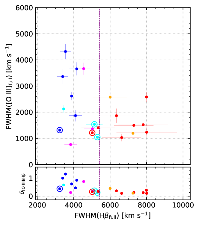
Figure 9: Top panel: FWHM of the full profile of [O III]$\lambda$5007 vs. FWHM of the full profile of H$\beta$. Bottom panel: Ratio $\delta_{\textrm{[O III]/H}\beta}=$ FWHM([O III]_full)/FWHM(H$\beta_{\rm full}$) vs. FWHM of the full profile of H$\beta$. As in Fig. 4, each colour represent one different spectral type, and symbols surrounded by open circles indicate the radio-loud quasars.

The relation between the FWHM of the full profiles of H$\beta$ and O III]$\lambda$5007 is shown in Fig. 9. In general, the two populations present a FWHM(H$\beta_{\rm{full}}$) higher than FWHM([O III]_full), as expected from previous observations (Sulentic et al., 2004, 2007; Zamfir et al., 2010, M09). At low-z, only in the case of the “blue-outliers” the [O III]$\lambda\lambda$4959,5007 profiles appear to be very boxy-shaped and with the FWHM $>1000$ km s^-1. Some of these sources are NLSy1s and the [O III]$\lambda\lambda$4959,5007 FWHM is becoming comparable to the one of the broad H$\beta$ profile sources (Zamanov et al., 2002; Komossa et al., 2008; Cracco et al., 2016; Komossa et al., 2018; Berton & Järvelä, 2021). At high $z$ and high luminosity the [O III]$\lambda\lambda$4959,5007 profiles often appear much broader, as do also the H$\beta$ broad profiles (Carniani et al., 2015; Fiore et al., 2017; Villar Martín et al., 2020). Two cases in point from previous works are 2QZJ002830.4-281706 at $z=2.$ (Cano-Díaz et al., 2012; Carniani et al., 2015) and HE0940-1050 at $z=3.1$ (Marziani et al., 2017a). We have four sources that present [O III]$\lambda\lambda$4959,5007 FWHM above 3000 km s^-1, comparable to the H$\beta$ FWHM, with one extraordinary case in which FWHM(H$\beta_{\rm{full}}$) is smaller than FWHM([O III]_full) (SDSSJ135831.78+050522.8, Pop. A1), with FWHM(H$\beta_{\rm{full}}$) $\approx 3550$ km s^-1 and FWHM([O III]_full) $\approx 4320$ km s^-1 (see Fig. 27). Although FWHM of [O III]$\lambda\lambda$4959,5007 $\gtrsim 2000$ km s^-1 are frequently observed at high luminosity, some extreme values should be taken with care because the [O III]$\lambda\lambda$4959,5007 profiles are weak and broad: it is difficult to properly define the [O III]$\lambda\lambda$4959,5007 profiles especially when the broad H$\beta$ red wing is strong.

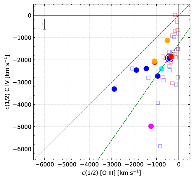
Figure 10: Centroid velocity at 1/2 flux intensity ($c$(1/2)) of C IV$\lambda$1549 vs. $c$(1/2) of [O III]$\lambda\lambda$4959,5007. Blue and red open squares show the HE Pop. A and Pop. B sources studied by M09 and S17. Color scheme as in Fig. 4. The green line indicates the linear regression between $c$(1/2) of C IV$\lambda$1549 and [O III]$\lambda\lambda$4959,5007 obtained through the orthogonal least square method. The error bars refer to 1$\sigma$ level of confidence for our sample.

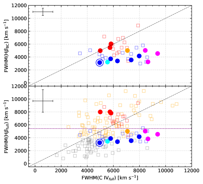
Figure 11: FWHM(H$\beta_{\rm{BC}}$) $vs.$ FWHM(C IV_full) and FWHM(H$\beta_{\mathrm{full}}$) $vs.$ FWHM(C IV_full). Sources are identified according to the different bins of spectral types following color scheme from Fig. 4. Blue and red open squares represent Pop. A and Pop. B sources from S17 and grey and orange open squares indicate Pop. A and Pop. B from S07, respectively. Horizontal purple line indicates the A/B boundary and the error bars on the top left of the plots refer to 1$\sigma$ level of confidence for our sample.

6.1.2 [O III]$\lambda\lambda$4959,5007 vs. C IV$\lambda 1549$

Fig. 10 shows the relation between $c$(1/2) for [O III]$\lambda\lambda$4959,5007 and C IV$\lambda$1549. The HE comparison sample analysed in M09 and S17 is included. The sources that present strong shifts in the [O III]$\lambda\lambda$4959,5007 emission line profiles will also present it in C IV$\lambda$1549, in agreement with the HE data. Both lines show a correlation between their widths and shifts (Fig. 6 for [O III]$\lambda\lambda$4959,5007 and Fig. 8 for C IV$\lambda$1549) indicating that the broadening is mainly associated with a blueshifted component that is increasing in prominence with increasing shift. The least squares linear regression of Fig. 10 (considering both HEMS and our sample) is given by:

$$c(1/2)_{\rm{C\textsc{IV}}}=(1.50\pm 0.31)\ c(1/2)_{\rm[{O\textsc{III}}]}+(-1239\pm 276),$$ (3)

in a good agreement with the study of Coatman et al. (2019). The trend (actually, a weak, marginally significant correlation at a $3\sigma$ confidence level) of Fig. 10 raises the issue of the relation between [O III]$\lambda\lambda$4959,5007 and C IV$\lambda$1549 outflows. There is evidence suggesting that the semi-broad component of [O III]$\lambda\lambda$4959,5007 $W$ remains almost constant with luminosity (Marziani et al., 2016b, Section 4.3), overwhelming the narrow, core component. The narrow component is however mainly associated with the NLR that may extend up to tens of kpc (Bennert et al., 2002, 2006). The dispersion in the relation with more sources around 0 shift in [O III]$\lambda\lambda$4959,5007 might be explained by a narrow component whose strength may depend on the past AGN evolution (Storchi-Bergmann et al., 2018). It is therefore not surprising that, even if a large C IV$\lambda$1549 shift is measured, the [O III]$\lambda\lambda$4959,5007 profile may be unshifted or show only a modest blueshift. However, the presence of a shift correlation and the relatively large [O III]$\lambda\lambda$4959,5007/C IV$\lambda$1549 FWHM ratio support a physical connection between an inner outflow on scales of a few hundreds gravitational radii where the BLUE C IV$\lambda$1549  component is emitted, and an outflow at the outer edge of the BLR, beyond $10^{4}-10^{5}$ gravitational radii (Zamanov et al., 2002) where the [O III]$\lambda\lambda$4959,5007 semibroad component likely originates. The nature of this connection remains unclear. It is beyond the scope of the present paper and might be investigated elsewhere.

6.1.3 C IV$\lambda 1549$ versus H$\beta$

Top panel of Fig. 11 represents the relation between FWHM(H$\beta_{\rm BC}$) and FWHM(C IV_full), including the S17 sample. Our data is in agreement with this comparison sample in terms of a clear A/B separation. Pop. A sources seem to present a trend from A1 to A3 in the FWHM(C IV_full) where the A3 sources show the largest values. The FWHM(C IV_full) is larger than the FWHM(H$\beta_{\rm BC}$), and the widths of the two lines are not correlated. There is a degeneracy between C IV$\lambda$1549 and H$\beta$: to a single value of H$\beta$ FWHM corresponds a wide range of C IV$\lambda$1549 FWHM (c.f. S07, Capellupo et al. 2015; Mejía-Restrepo et al. 2016; Coatman et al. 2017). The systematically broader profile can be interpreted as a consequence of the dominance of the outflow component in the C IV$\lambda$1549 line profile (Marziani et al., 2019).

The bottom panel of Fig. 11 shows the FWHM(C IV_full) vs. FWHM(H$\beta_{\rm full}$) where, apart from including S17 data, we also display the low-$z$ sample from S07 for comparison. In this plot, the separation between Pop. A and Pop. B is even clearer: Pop. A sources show broader C IV$\lambda$1549, while those of Pop. B have values consistent with, or narrower, than H$\beta$.

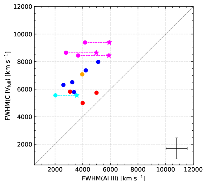
Figure 12: C IV_full relation with Al III$\lambda$1860. Colour scheme as in Fig. 4. The data points joined by a dashed line are those for which a significant blueshifted emission component has been isolated. The left data points refer to the Al III$\lambda$1860 BC only and the right ones (star symbol) to the full profile FWHM (BC+BLUE). Error bars refer to 1$\sigma$ level of confidence.

6.1.4 C IV$\lambda 1549$ versus Al III$\lambda$1860

Fig. 12 shows FWHM of the full profiles of C IV$\lambda$1549 vs. FWHM of Al III$\lambda$1860. The FWHM(C IV_full) presents significantly higher values than FWHM(Al III). This indicates that the relation between C IV$\lambda$1549 and Al III$\lambda$1860 is similar to the one of C IV$\lambda$1549 and H$\beta$. In both cases the C IV$\lambda$1549 FWHM tends to be larger: always significantly so for Pop. A, and larger or consistent for Pop. B. The cyan and magenta dashed lines connect the FWHM estimated from the Al III$\lambda$1860 BC with and without a BLUE component: without the BLUE (stars), the Al III$\lambda$1860 FWHM becomes closer to, but remains significantly smaller than the FWHM of the C IV$\lambda$1549 full profile.

6.2 Virial black hole mass estimates

A comparison between the FWHM of Al III$\lambda$1860 and H$\beta$ (BC and full) profiles is shown in Fig. 13. The figure includes the data from Marziani et al. (2022c, hereafter M22) that involve exclusively Pop. A sources. The FWHM of H$\beta_{\rm{BC}}$ is consistent with the FWHM of Al III$\lambda$1860 for Pop. A: their average ratio (FWHM Al III over FWHM H$\beta$) in our sample is $\approx 0.87\pm 0.18$. The right panel of Fig. 13 shows a comparison between FWHM(Al III) vs. FWHM of full H$\beta$. The purple dotted vertical line indicates the A/B boundary as in Fig. 3. The location of our Pop. A objects remains in agreement with the results from M22, and with those for H$\beta_{\rm{BC}}$. There is a clear deviation from the 1:1 line in the location of Pop. B sources: for the 5 Population B sources of our sample the average ratio is just $0.57\pm 0.12$ (c.f. Marziani et al. 2017b). These results provide evidence that Pop. B Al III$\lambda$1860 is systematically narrower than H$\beta$ full profile, most likely because of the strong VBC contribution. The ratio FWHM Al III$\lambda$1860 over H$\beta_{\rm{BC}}$  is in fair agreement $\approx 0.79\pm 0.16$ for Pop. B, and therefore the H$\beta$ VBC should not be included on the black hole mass estimation. The 20 % difference between the FWHM H$\beta_{\rm{BC}}$ and FWHM Al III$\lambda$1860 for Pop. B sources is marginally significant and should be confirmed by larger samples.

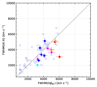
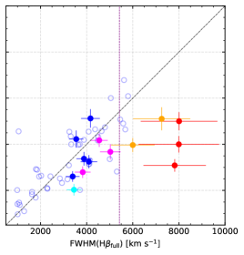
Figure 13: FWHM(Al III) $vs.$ FWHM(H$\beta_{\rm{BC}}$) (left panel) and FWHM(Al III) $vs.$ FWHM(H$\beta_{\mathrm{full}}$) (right panel). Sources are identified according to the different bins of spectral types following colour scheme from Fig. 4. Blue open circles show the data from M22 Pop. A sources for a comparison. Vertical purple line indicates the A/B boundary for our sample.

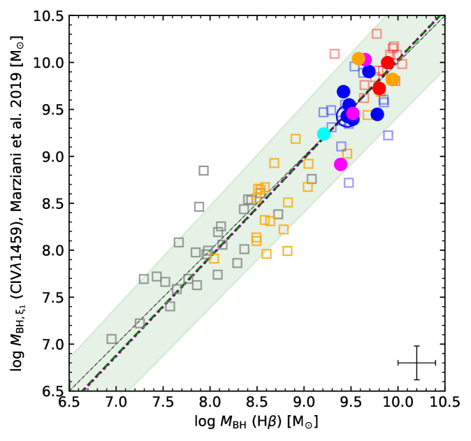
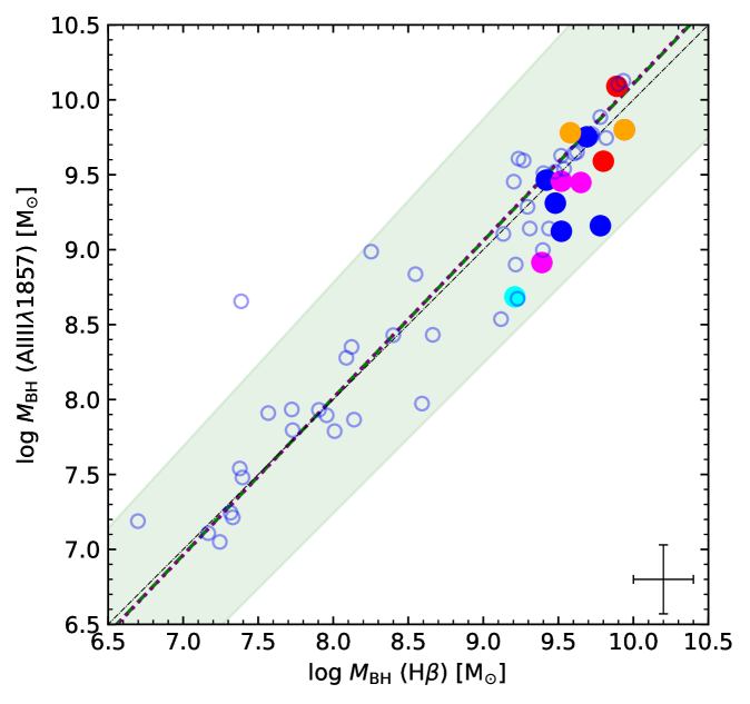
Figure 14: $M_{\rm BH}$(H$\beta$) compared to $M_{\rm BH}$(C IV) (left panel) and to $M_{\rm BH}$(Al III) (right panel). Open squares on the left plot represent the low- and high-redshift sources analysed by Marziani et al. (2019) (blue and red for high-$z$ and grey and orange for low-$z$ Pop. A and Pop. B, respectively). Blue dots on the right panel are for the M22 data. Green and purple dashed lines indicate the linear regressions using bisector and orthogonal methods, respectively. Colour scheme as in Fig. 4.

The black hole masses are estimated through different scaling relations using emission lines such as those based on the FWHM of H$\beta$, Al III$\lambda 1860$, and C IV$\lambda 1549$. The scaling law of Vestergaard & Peterson (2006) was used to estimate the mass $M_{\rm BH}$ with FWHM H$\beta_{\rm{BC}}$. We utilize Equation (18) from Marziani et al. (2019, $\sigma=0.33$) to estimate $M_{\textrm{BH}}$ with the C IV$\lambda 1549$ FWHM.

The left panel of Fig. 14 presents a comparison between the $M_{\textrm{BH}}$ estimates using the scaling law for C IV$\lambda 1549$ from Marziani et al. (2019) and the H$\beta$ scaling law of Vestergaard & Peterson (2006). The open squares in this plot indicate the data from Marziani et al. (2019) which include high- and low-$z$ sources. Our sample agrees with the previous estimates and corresponds to the extreme cases, with the largest $M_{\textrm{BH}}$ reaching $10^{10}$ M_⊙.

The plot of $M_{\textrm{BH, Al III}}$ vs. $M_{\textrm{BH, H$\beta$}}$ (right panel of Fig. 14). relies on the $M_{\rm BH}$ scaling law from M22. The $M_{\rm BH,H\beta}$ and $M_{\rm BH,{Al\textsc{III}}}$ values obtained for our sources are compatible within the confidence interval of the M22 scaling law for Al III$\lambda$1860. We caution that the relation given in this equation has been derived for Pop. A sources and, consequently, it may lead to larger uncertainties for Pop. B quasars. For these sources we apply a correction $\xi=\rm{FWHM}_{\rm{H\beta,BC}}/\rm{FWHM}_{\rm{{Al\textsc{III}}}}=1.35\pm 0.10$ to the FWHM(Al III) (Marziani et al., 2017a, who assumed FWHM H$\beta_{\rm{BC}}$ as the reference virial broadening estimator).

The equations that describe the relations between $M_{\rm BH}$ estimations using $\xi$-corrected C IV$\lambda$1549 and Al III$\lambda$1860 are listed in Table 12. Col. 1 lists the method used for the linear regression (orthogonal and bisector); Cols. 2 and 3 present the linear and angular coefficients together with the respective standard deviations; rms error and Pearson correlation coefficient $r$ are reported in Cols. 4 and 5, respectively.

The original C IV$\lambda$1549 VP06 relation lacks a correction because of the bias introduced by non-virial broadening (i.e., by the blueshifted component; Brotherton et al. 2015; Coatman et al. 2017; Marziani et al. 2019). If $M_{\rm BH}$ estimated with the uncorrected VP06 relations are used, there is a significant deviation in the 1:1 relation between H$\beta$ and C IV$\lambda 1549$ $M_{\rm{BH}}$ estimates and a large scatter (rms $\approx 0.42$). We therefore utilise the scaling laws based on Al III$\lambda$1860 and $\xi$-corrected C IV$\lambda$1549 that may provide less biased estimators with respect to H$\beta$-based $M_{\rm BH}$ scaling law.

Table 12: Linear relations between the different $M_{\rm BH}$ estimates using orthogonal and bisector methods.

Method	$a\pm\delta a$	$b\pm\delta b$	RMS	CC
(1)	(2)	(3)	(4)	(5)
$M_{\rm BH,CIV,M19}=a+b*M_{\rm BH,H\beta,VP06}$
Orthogonal	$-0.495\pm 0.306$	$1.053\pm 0.034$	0.315	0.949
Bisector	$-0.471\pm 0.289$	$1.050\pm 0.032$
$M_{\rm BH,AlIII,M22}=a+b*M_{\rm BH,H\beta,VP06}$
Orthogonal	$-0.389\pm 0.431$	$1.050\pm 0.047$	0.320	0.948
Bisector	$-0.366\pm 0.411$	$1.047\pm 0.045$

Table 13: Weighted averaged masses, luminosity at 5100 Å, and Eddington ratio ($L/L_{\rm Edd}$), in logarithmic scale.

Source	$M_{\rm BH,H\beta}$	$M_{\rm BH}$	$L$(1450Å)	$L$(5100Å)	$L/L_{\rm Edd}$
(1)	(2)	(3)	(4)	(5)	(6)
Population A
SDSSJ005700.18+143737.7	9.39 $\pm$ 1.41	9.37 $\pm$ 0.27	46.65 $\pm$ 5.60	46.41 $\pm$ 5.57	0.10 $\pm$ 0.01
SDSSJ132012.33+142037.1	9.21 $\pm$ 1.38	9.19 $\pm$ 0.14	46.74 $\pm$ 5.61	46.42 $\pm$ 5.57	0.03 $\pm$ 0.01
SDSSJ135831.78+050522.8	9.42 $\pm$ 1.41	9.56 $\pm$ 0.11	46.97 $\pm$ 5.64	46.67 $\pm$ 5.60	0.07 $\pm$ 0.01
Q 1410+096	9.52 $\pm$ 1.43	9.42 $\pm$ 0.20	47.11 $\pm$ 5.65	46.92 $\pm$ 5.63	0.32 $\pm$ 0.04
B1422+231(a)	9.96 $\pm$ 1.49	-	-	47.07 $\pm$ 5.65	-0.07 $\pm$ 0.01
SDSSJ161458.33+144836.9	9.48 $\pm$ 1.42	9.49 $\pm$ 0.10	47.05 $\pm$ 5.65	46.69 $\pm$ 5.60	0.04 $\pm$ 0.01
PKS 1937-101(a)	10.14 $\pm$ 1.52	-	-	47.36 $\pm$ 5.68	0.05 $\pm$ 0.01
PKS 2000-330	9.46 $\pm$ 1.42	9.21 $\pm$ 0.04(c)	46.58::	46.94 $\pm$ 5.63	0.30 $\pm$ 0.04
SDSSJ210524.47+000407.3	9.84 $\pm$ 1.48	9.83 $\pm$ 0.28(b)	47.16 $\pm$ 5.66	46.89 $\pm$ 5.63	-0.13 $\pm$ 0.02
SDSSJ210831.56-063022.5	9.52 $\pm$ 1.43	9.63 $\pm$ 0.12	46.98 $\pm$ 5.64	46.43 $\pm$ 5.57	-0.26 $\pm$ 0.03
SDSSJ212329.46-005052.9	9.69 $\pm$ 1.45	9.77 $\pm$ 0.08	47.19 $\pm$ 5.66	46.92 $\pm$ 5.63	0.05 $\pm$ 0.01
SDSSJ235808.54+012507.2	9.78 $\pm$ 1.47	9.57 $\pm$ 0.31	46.85 $\pm$ 5.62	47.11 $\pm$ 5.65	0.15 $\pm$ 0.02
Population B
HE 0001-2340(a)	9.63 $\pm$ 1.44	-	-	46.48 $\pm$ 5.58	-0.33 $\pm$ 0.04
$[\rm HB89]$ 0029+073(a)	9.71 $\pm$ 1.46	-	-	46.81 $\pm$ 5.62	-0.07 $\pm$ 0.01
CTQ 0408(a)	10.20 $\pm$ 1.53	-	-	47.26 $\pm$ 5.67	-0.12 $\pm$ 0.01
H 0055-2659(a)	9.69 $\pm$ 1.45	-	-	46.75 $\pm$ 5.61	-0.12 $\pm$ 0.01
SDSSJ114358.52+052444.9	9.58 $\pm$ 1.44	9.75 $\pm$ 0.25	47.16 $\pm$ 5.66	46.39 $\pm$ 5.57	-0.05 $\pm$ 0.01
SDSSJ115954.33+201921.1	9.89 $\pm$ 1.48	9.90 $\pm$ 0.05	47.36 $\pm$ 5.68	46.84 $\pm$ 5.62	-0.23 $\pm$ 0.03
SDSSJ120147.90+120630.2	9.94 $\pm$ 1.49	9.89 $\pm$ 0.2	47.19 $\pm$ 5.66	47.09 $\pm$ 5.65	0.03 $\pm$ 0.01
SDSSJ141546.24+112943.4	9.80 $\pm$ 1.47	9.78 $\pm$ 0.07(b)	47.08 $\pm$ 5.65	46.64 $\pm$ 5.60	-0.33 $\pm$ 0.04
SDSSJ153830.55+085517.0	9.80 $\pm$ 1.47	9.76 $\pm$ 0.24	47.23 $\pm$ 5.67	46.50 $\pm$ 5.58	-0.47 $\pm$ 0.06
PKS 2126-15(a)	9.78 $\pm$ 1.47	-	-	47.11 $\pm$ 5.65	0.16 $\pm$ 0.02

Table 13 lists the individual values of H$\beta$ black hole masses (Col. 2), the weighted averages of $M_{\rm BH}$ (Col. 3), the luminosity at 1450Å and 5100Å (Cols. 4 and 5, respectively), as well as the Eddington ratio of each source (Col.6). We have considered the mass estimates using H$\beta$, Al III$\lambda$1860, and C IV$\lambda$1549 to determine the weighted average of $M_{\rm BH}$ and used the FWHM errors as weights. H$\beta$ $M_{\rm BH}$ are also reported since they are available for all sources of our sample and needed to compare our data to previous samples. We have adopted a bolometric correction of 10 for the optical range in accordance with the value assumed in the previous works we consider for comparison (e.g., Richards et al. 2006; ; ; , ), although lower bolometric corrections are expected in the $L_{\rm bol}>10^{47}$ erg s^-1 luminosity range (Marconi et al., 2004; Netzer, 2019), which may introduce a bias towards higher accretion rates. The bolometric correction adopted in the UV range is 3.5 (Elvis et al., 1994).

6.3 Dependence on accretion parameters

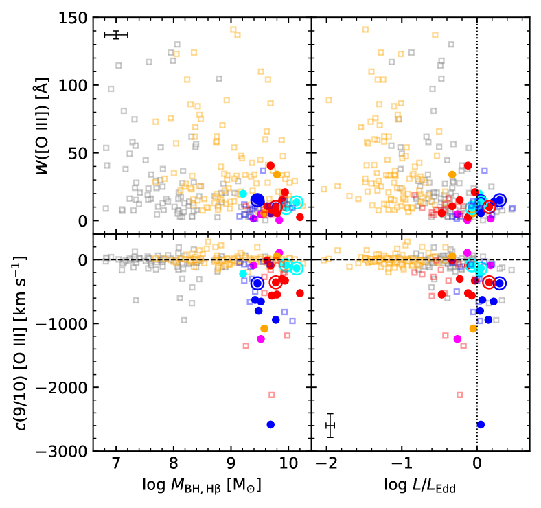
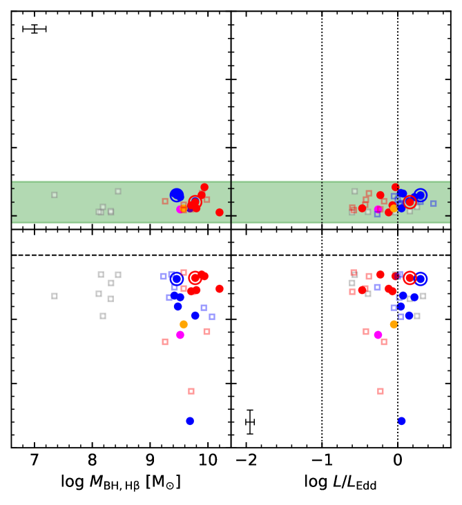
Figure 15: [O III]$\lambda\lambda$4959,5007 dependence on physical parameters. Left panel: Our full sample in comparison with the full M03 (grey for Pop. A and orange for Pop. B) and HE (blue for Pop. A and red for Pop. B) samples. Right panel: Only sources with $c$(9/10) $<-250$ km s^-1. Our data follow the same colour scheme as in Fig. 4.

6.3.1 [O III]$\lambda\lambda$4959,5007

Fig. 15 shows the dependence of $W$([O III]) and $c$(9/10) [O III] on M_BH,Hβ and L/L_Edd. Our sample presents $W$([O III]) $<25$Å in the majority of the cases, with only two outliers (SDSSJ141546.24+112943.4 with $\approx$ 34Å and H 0055-2659 with $\approx$ 41Å). The $W$([O III]) of our sample is relatively small when compared with low-$z$ sources. However, our data show more frequently blueshifts in $c$(9/10).

The right panels of Fig. 15 consider only sources that present $c$(9/10) $<-250$ km s^-1. In this case, all the sources fit within $W(\rm[{O\textsc{III}}])\lesssim 25$Å and are found in a wide range of $M_{\rm BH}$ as for the distribution of the full samples. Sources with $c$(9/10) $<-250$ km s^-1 have an average Eddington ratio of -0.09: at high Eddington ratios the [O III]$\lambda\lambda$4959,5007 profiles tend to be strongly affected or dominated by the blueshifted SBC. In addition, the [O III]$\lambda\lambda$4959,5007 $W$ remains roughly constant over a wide range of masses (and luminosity), indicating that the luminosity of the blueshifted SBC is proportional to the continuum luminosity. This result provides evidence that the outflow traced by the blueshifted [O III]$\lambda\lambda$4959,5007 is directly related to the active nucleus, as proportionality between line and continuum luminosity is a classical proof of photoionisation (Osterbrock & Shuder, 1982).

6.3.2 C IV$\lambda$1549

In Fig. 16, we provide an analysis of the dependence of C IV$\lambda$1549 shift measured by $c$(1/2) on luminosity and $L/L_{\rm Edd}$. We include the data analysed by Marziani et al. (2019) along with the present sample data. The same trend appears to be followed by both ours and Marziani et al. (2019) samples. Sources that present the largest values of C IV$\lambda$1549 $c$(1/2) are Population A, with two xAs (SDSSJ210524.47+000407.3 and SDSSJ210831.56-063022.5) reaching $c$(1/2) $\approx$ –5000 km s^-1.

As in S17, the left plot of Fig. 16 indicate a clear relation (with a Pearson correlation coefficient of 0.59) between $c$(1/2) of C IV$\lambda$1549 and $L/L_{\rm Edd}$, given by the following equation for the absolute value of the centroid shift at 1/2:

$$\log|c(1/2)|_{\rm{C\textsc{IV}}}=(0.43\pm 0.06)\log L/L_{\rm Edd}+(3.25\pm 0.04).$$ (4)

A similar relation can also be derived between the absolute value of C IV$\lambda$1549 $c$(1/2) and $L_{\rm bol}$(1450Å) (right panel of Fig. 16):

$$\log|c(1/2)|_{\rm{C\textsc{IV}}}=(0.18\pm 0.03)\log L_{\rm bol}+(-5.70\pm 1.46).$$ (5)

The Pearson correlation coefficient in this case is 0.54. These relations are consistent with those of S17 who found slope $\approx 0.5$ and $\approx 0.2$ for the dependence on Eddington ratio and luminosity, respectively. Since the S17 data were included in the linear regression, we can say that the new data confirm the slope difference that suggests a major role of the $L/L_{\rm Edd}$ for governing the shift amplitude, and a secondary effect of luminosity.

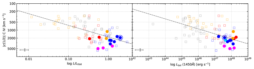
Figure 16: Left panel: Relation between C IV $c$(1/2) and $L/L_{\rm{Edd}}$. Right panel: C IV $c$(1/2) vs. $L_{\rm bol}$(1450Å). Grey and orange squares represent low-$z$ Pop. A and Pop. B quasars respectively, while blue and red open squares indicate HE Pop. A and Pop. B sources from S17. Color scheme as Fig. 4. Linear regressions are shown by the dashed lines. The errors refer only to our sample.

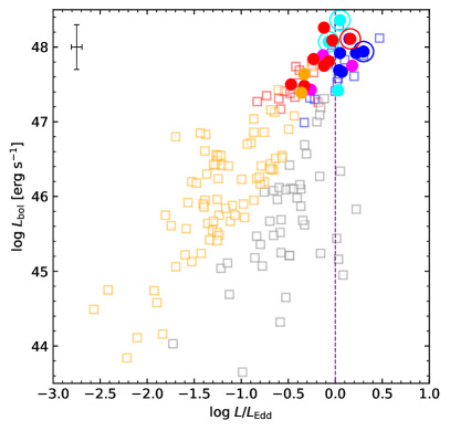
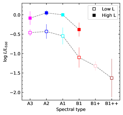
Figure 17: Left plot: Bolometric luminosity $L_{\rm bol}$ versus Eddington ratio ($L/L_{\rm Edd}$). Squared symbols identify the samples of S07 (low-$z$) and of S17 (high-$z$ sources). Vertical purple line indicates $L/L_{\rm Edd}=1$. Colour scheme as in Fig. 4. Right plot: Median values of the Eddington ratio separated into high-luminosity ($\log L>47$ erg s^-1) and low luminosity for each spectral type. We have included our own sources together with the comparison samples. Error bars indicate the semi-interquartile range.

6.4 Redefining optical properties of high-$z$ sources

Fig. 17 shows the relation between the Eddington ratio and the bolometric luminosity. The distinction between Pop. A and Pop. B is very clear in both low- and high-redshift samples including our sample, and the data analysed by S07 and S17. The systematically higher Eddington ratio of the high-luminosity samples may be in part the result of a Malmquist type bias (Sulentic et al., 2014), of the assumption of a constant bolometric correction over a wide range in luminosity, of orientation effects, and of intrinsic evolution of the Eddington ratio (e.g., Cavaliere & Vittorini, 2000; Volonteri et al., 2003; Shankar et al., 2009). For instance, the radio-loud sources from our sample seem to be the more extreme cases of their respective population, reaching $L/L_{\rm Edd}\sim 1$. They are core-dominated and presumably beamed in the direction of the observer. The line profiles appear composite, in the sense that they show a narrower core superimposed on a VBC. The width of the narrower core may be lowered if the emitting regions are constrained within a flattened geometry that is seen pole-on. This effect blurs the distinction between Pop. A and B, letting sources that are intrinsically Pop. B enter into the domain of Pop. A in the MS optical plane (Fig. 3; Marziani et al. 2001; Zamfir et al. 2008).

The right panel of Fig. 17 presents the median values of the Eddington ratio for each individual spectral type, distinguishing between higher ($L>10^{47}$ erg s^-1) and lower ($L<10^{47}$ erg s^-1) luminosity sources ( ; ; , together with our sample). The Eddington ratio is consistently higher in Pop. A sources rather than in Pop. B sources for both cases of luminosity and redshift separation. Low-redshift, low-luminosity sources present very small $L/L_{\rm Edd}$ values for Pop. B. The more extreme case is for low-redshift Pop. B1++, with a $L/L_{\rm Edd}\approx-1.65$. On the converse Pop. A sources have more similar values at low and high luminosity. There is no notable difference between high/low-luminosity and high/low-redshift distribution on the spectral type and log L/L_Edd plane, which may indicate that the more luminous sources present the highest Eddington ratios because of a Malmquist-type bias (Sulentic et al., 2014) rather than evolutionary effects on $L/L_{\rm Edd}$.

Of the four quasars that are radio-loud, B1422+231, PKS 1937-101, and PKS 2000-330 are classified as Pop. A while PKS 2126-15 is a Pop. B source. From four sources we can only make some preliminary considerations that will be properly discussed in a companion paper involving mainly radio-loud objects. The basic result is that the four RLs do not have outstanding properties with respect to the RQ samples considered in this paper. They share the trends between H$\beta$ and [O III]$\lambda\lambda$4959,5007 RQ profile parameters. A remarkable aspect is that the four RL AGN studied in this paper show high Eddington ratio, a fact that is never observed in powerful RL sources at low-$z$ (Sikora et al., 2007; Zamfir et al., 2008) that are more frequently classified as population B sources. At low-$z$, low-power, “jetted” sources for which high Eddington ratio has been estimated to be $\sim$ 1 are known to exist (the so-called RL NLSy1s; Komossa et al., 2006; Berton et al., 2015; Foschini et al., 2015). Even if $L/L_{\rm Edd}$ might be overestimated, the implication is that there is apparently no empirical inconsistency between powerful jetted emission, and high accretion rate.

7 Conclusions

We presented a sample of 22 high-redshift and high-luminosity quasars (12 Pop. A; 10 Pop. B) observed with the VLT/ISAAC spectrograph to cover the H$\beta$ spectral range shifted into the near infrared. A dedicated analysis has been performed on the most prominent emission features in the new optical spectra (H$\beta$, [O III]$\lambda\lambda$4959,5007, Fe II), as well as in survey or published UV spectra (Al III$\lambda$1860, C III]$\lambda$1909, C IV$\lambda$1549, Si IV$\lambda$1397, Fe iii, Fe III$\lambda$1914), to measure several parameters related to the emitting gas physical conditions and dynamics.

The main conclusions are as follows.

1. We confirm that the full profile of H$\beta$ can be in general well represented by only a Lorentzian BC for Pop. A quasars, while for the Pop. B ones two Gaussians (BC and VBC) provide a satisfactory fit, with the broader, redshifted VBC accounting for $\approx 50$% of the emission line. Also, some Pop. A H$\beta$ profiles from our sample present outflowing components that seem to be related to those observed in the [O III]$\lambda\lambda$4959,5007 lines;

2. Compared to low-$z$ and low-luminosity samples, our data presents a displacement in the MS in the direction of higher values of FWHM of the H$\beta$ full profile and $R_{\rm{{Fe\textsc{II}}}}$. The relation between profile parameters and the $M_{\rm BH}$ and $L/L_{\rm Edd}$ differences between Pop. A and B are also confirmed, in the form seen in previous high-luminosity samples;

3. The [O III]$\lambda\lambda$4959,5007 profile is broad and not reproducible with a simple Gaussian. All [O III]$\lambda\lambda$4959,5007 profiles of our sample are blueshifted by more than 250 km s^-1. Differently from the low $z$ range, high-$z$ Pop. B [O III]$\lambda\lambda$4959,5007 profiles present significant contribution of blueshifted semi-broad components, even though they are still less strong than the ones found in Pop. A sources. Nevertheless, both population seem to share similar asymmetry indexes, which indicates that their profiles present comparable shapes;

4. In some cases [O III]$\lambda\lambda$4959,5007 FWHM reach values comparable to those of H$\beta$. This effect is found especially in sources with high $L/L_{\rm Edd}$, and may be compared with the case of highly-accreting NLSy1s at low $z$. Line widths appear extraordinarily large (thousands km s^-1) because of the high black hole mass values involved. [O III]$\lambda\lambda$4959,5007 correlations between FWHM and shift, and also between $W$ and shift mirror the correlations seen in C IV$\lambda$1549;

5. The [O III]$\lambda\lambda$4959,5007 lines should be avoided for accurate redshift estimates in high-$L$, high-$z$ quasars, as in most of sources the [O III] lines are dominated by a blueshifted SBC and no rest-frame narrow component could be clearly identified. The average shift of the [O III] profile peak is $\sim-520$ km s^-1, which may lead to a considerable systematic blueshift of $\delta z\sim 0.0017$ on the redshift estimation;

6. Several C IV$\lambda$1549 correlations (most notably the one between shift and width) and the C IV$\lambda$1549 parameters’ dependence on Eddington ratio and mass (or luminosity) are confirmed (including the ones of S17). Outflow-dominated profiles tend to have low-$W$, large FWHM and shifts. The three parameters are definitely related;

7. We exploit the VP06 scaling law as reference for $M_{\rm BH}$ estimates, and we verified that the scaling law based on Al III$\lambda$1860 is a reliable estimator with respect to black hole masses derived from H$\beta$. The C IV$\lambda$1549 scaling law requires a FWHM correction;

8. [O III]$\lambda\lambda$4959,5007 and C IV$\lambda$1549 seem to follow a very similar, strong correlation between FWHM and shift, measured by the $c$(1/2). The [O III]$\lambda\lambda$4959,5007 and C IV$\lambda$1549  outflow velocities are related, as suggested by the correlation between their shift amplitudes shown in Fig. 10;

9. The radio loud sources in the high-$z$ range seem to be radiating at high values of Eddington ratio (with $L/L_{\rm Edd}$ $\sim 1$), at variance with low-$z$ where the most powerful jetted sources belong to Population B and radiate at modest Eddington ratio.

The sample studied in this paper is the first part of a sample involving roughly an equal number of RQ and of RI and RL sources. The data in this paper provide a RQ comparison sample for the ISAAC spectra of RL sources that will be presented in a future paper.

Appendix A Multicomponent fits in the optical and UV ranges and individual notes

In this appendix we present the new VLT/ISAAC infrared spectra and the multi-component fittings for the optical spectral range, including the fits of H$\beta$+[O III]$\lambda\lambda$4959,5007. An additional analysis of the UV spectra is also presented for the objects with available UV spectra, from the literature or from SDSS. The UV analysis includes fittings for Si IV$\lambda$1397+O IV]$\lambda$1402, C IV$\lambda$1549+He II$\lambda$1640 as well as for the 1900 Å blend. We also include notes for some of the individual objects.

A.1 HE 0001-2340

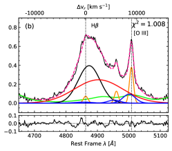
Figure 18: HE 0001-2340. (a) Rest-frame spectrum covering the H$\beta$ spectral range obtained with VLT/ISAAC. The spectrum is normalised by the continuum at 5100Å (the flux values are available at Table 4). The grey dashed line traces a power law that defines the continuum level as obtained with the specfit multicomponent analysis. The green line shows the Fe II contribution. For this object Fe II was fitted only with the red Fe II blend due to the presence of atmospheric absorption in the blue. The vertical dotted lines indicate the rest-frame of the main emission lines in the H$\beta$ spectral range and the grey-shaded area indicate the regions that were not considered in the fittings. The white area indicates the region used to anchor both the continuum and the Fe II template. (b) Result of the fitting after continuum subtraction (upper panel) and the residuals (bottom panel) for the H$\beta$ region. Pink dashed line shows the final fit. Broad H$\beta$ component (BC) is represented by a black line meanwhile red line show the VBC. Orange lines represent narrow components and the blue ones correspond to the blueshifted components. The region in which the Fe II template was fitted is represented by the solid green line. Dotted green line indicate the expected Fe II contribution for the other parts of the spectra.

A.2 $[\rm HB89]$ 0029+073

Jaunsen et al. (1995) list this source as a gravitational lens candidate. $[\rm HB89]$ 0029+073 is another case in which the Fe II contribution was measured at $\lambda\geq$ 5000Å, and rescaled to obtain the intensity of Fe II$\lambda 4570$ blend.

A.3 CTQ 0408

As in the case of $[\rm HB89]$ 0029+073, the Fe II of CTQ 0408 was fit on the red side of H$\beta$ with $\lambda\geq$ 5000Å.

Radio information about this source was found only in the SUMSS catalogue (Mauch et al. 2003). There is no radio map from NVSS nor FIRST for this object, because it is out of the respective survey fields.

A.4 SDSSJ005700.18+143737.7

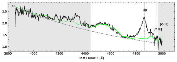
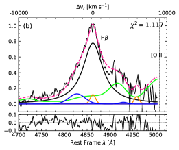
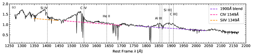
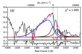
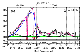
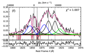
Figure 21: SDSSJ005700.18+143737.7. Top panels: Same as Fig. 18. (c) continuum-normalised UV spectrum from SDSS DR-16 with adopted continuum marked in colour; Bottom panels: fits for (d) Si IV$\lambda$1397+O IV]$\lambda$1402, (e) C IV$\lambda$1549+He II$\lambda$1640, and (f) the 1900 Å blend. Pink dashed lines show the final fitting. Broad components are represented by black lines, while blueshifted components are in blue. Green line represents the additional Fe III$\lambda$1914 line in the red side of C III], observed in extreme Pop. A sources. Brown lines represent the absorptions seen in the spectrum and modelled as negative-flux Gaussians.

H$\beta$+[O III]$\lambda\lambda$4959,5007 falls at the red border of the observed spectrum. Consequently, the [O III] measurements should be treated as highly uncertain and special marks have been included in the corresponding tables in the paper. The measurements and the analysis on the [O III] profile were performed with the [O III]$\lambda$4959 instead of [O III]$\lambda$5007. With respect to the UV spectrum, the object presents strong absorption lines likely associated with intervening absorbers throughout the three UV regions of interest. In the analysis we also included Gaussians profiles for the absorption lines in the fittings. It was necessary to include two blueshifted components for Al III$\lambda$1860 and Si III]$\lambda$1892, otherwise both Al III$\lambda$1860 and Si III]$\lambda$1892 BC are shifted by more than 1000 km s^-1.

A.5 H 0055-2659

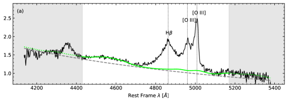
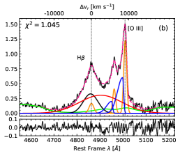
Figure 22: H 0055-2659. Same as Figure 18.

The VLT rest-frame optical spectrum of H 0055-2659 presents a very flat profile and small Fe II multiplets contributions.

A.6 SDSSJ114358.52+052444.9

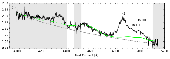
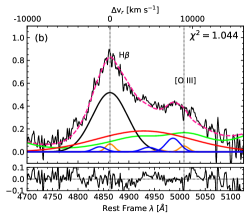
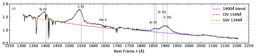
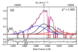
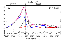
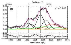
Figure 23: SDSSJ114358.52+052444.9. Top panels: same as Fig. 18 Middle and bottom panels: same as Fig. 21. Pink dashed lines show the final fitting. Broad components are represented by black lines, while blueshifted components are in blue. Brown lines represent the absorption lines seen in the spectrum.

A.7 SDSSJ115954.33+201921.1

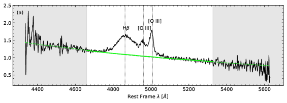
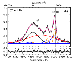
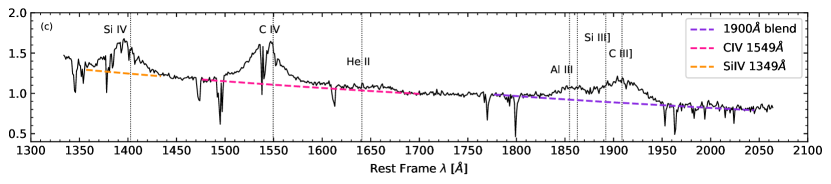
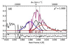
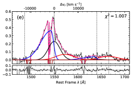
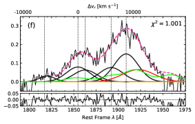
Figure 24: SDSSJ115954.33+201921.1. Same as Figure 23.

In the optical range, this source presents a very flat spectrum and almost no Fe II contributions.

A.8 SDSSJ120147.90+120630.2

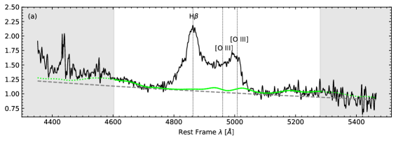
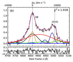
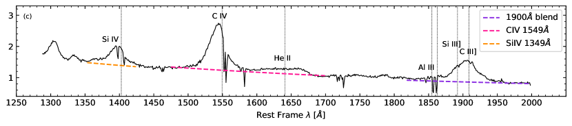
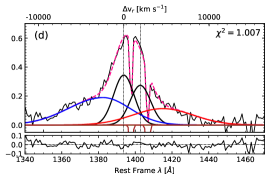
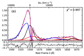
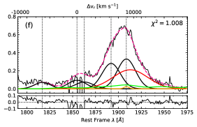
Figure 25: SDSSJ120147.90+120630.2. Same as Figure 23.

This quasar has observations of the H$\beta$ region at the Large Binocular Telescope (LBT), as reported in Bischetti et al. (2017). We stress that their spectrum is very similar to the one of ISAAC/VLT.

A.9 SDSSJ132012.33+142037.1

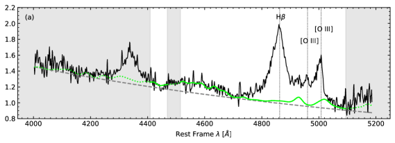
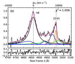
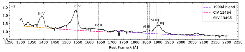
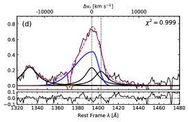
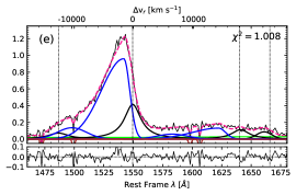
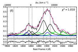
Figure 26: SDSSJ132012.33+142037.1. Same as Figure 23.

A.10 SDSSJ135831.78+050522.8

A.11 Q 1410+096

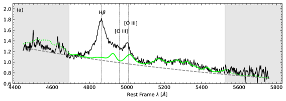
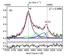
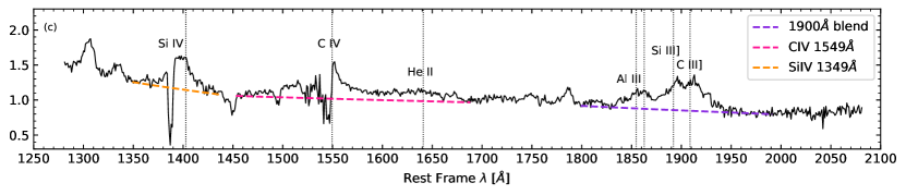
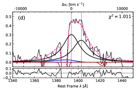
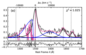
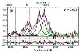
Figure 28: Q 1410+096. Same as Figure 23.

This source has been identified as a BAL quasar by Allen et al. (2011) and the absorption lines are seen in the regions of the Si IV$\lambda$1397 and C IV$\lambda$1549 emission lines. In order to account for the multiplet contributions in the optical region, we performed a fitting of this Fe II emission on the red side of H$\beta$, since the blue part of the FeII$\lambda$4570 region is close to the border of the spectrum and evidently affected by background subtraction or telluric absorption correction.

For this quasar, we perform the fitting of the C IV$\lambda$1549 line based on the He II$\lambda$1640 profile. The Al III$\lambda$1860 BC of 1410+096 is narrow when compared to H$\beta$, which may indicate that H$\beta$ might be affected by blueshifted emission. An excess (not included in the fit) is also visible on the blue side of Al III$\lambda$1860 (bottom rightmost panel of Fig. 28).

This source has also been analysed in detail in Deconto-Machado et al. (2022).

A.12 SDSSJ141546.24+112943.4

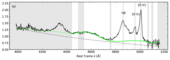
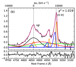
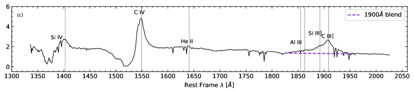
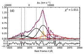
Figure 29: SDSSJ141546.24+112943.4. Top panels: Colours and lines as in Fig. A.1. (c) UV spectrum. (d) Fittings for the 1900 Å blend. Pink dashed lines show the final fitting. Broad components are represented by black lines, while narrow and very broad components are in orange and red, respectively. Brown lines represent the absorption seen in the spectrum.

This object is known as a weak microlensing candidate in the literature (Sluse et al. 2012; Takahashi & Inoue 2014). According to Welling et al. (2014), the quasar is a gravitationally lensed object split into 4 images separated by $\sim$ 1”. SDSSJ141546.24+112943.4 is a modest core-dominated radio-loud source with a logarithmic radio loudness parameter of 1.09.

As can be seen in the UV spectra presented in Fig. 29, the source is a BAL quasar, with broad absorption lines especially in the C IV$\lambda$1549 and Si IV$\lambda$1397 regions. Hazard et al. (1984) also report broad absorption lines in Al III$\lambda$1860 that we can see on the blue side of the blend at $\lambda\approx 1820$ Å.

A.13 B1422+231

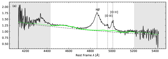
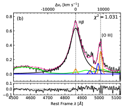
Figure 30: B1422+231. Colours and lines as in Figure 18.

The source has been studied in detail for the first time by Patnaik et al. (1992). It consists of a gravitationally lensed system with a diameter of 1.3 arcsec and four non-resolved components from VLA observations. This quasar is lensed into four images by a galaxy with $z=0.34$ (Tonry 1998). Dadina et al. (2016) used XMM-Newton to study the matter inflow at the centre of this source and found that its X-ray spectrum is quite similar to the one of a typical Seyfert galaxy. Several UV spectra were found in literature (Tonry 1998; Assef et al. 2011; Kundic et al. 1997; O’Dowd et al. 2017), but are not available for public usage or do not correspond to the regions we want to analyze. No SDSS spectrum was found. It has also been analysed in the infrared by Lawrence et al. (1992) who conclude that the source presents similar structures in both radio and infrared. This is one of the radio-loud sources from our sample.

A.14 SDSSJ153830.55+085517.0

When compared with the other sources of the sample, this source presents one of the spectra with lowest S/N. The low S/N might be due to the presence of a star that is located very close to the field of the quasar significantly increasing the background of the spectrum. This also may explain why the UV and the optical spectra of SDSSJ153830.55+085517.0 differ so much: while the optical spectrum shows a Pop. B-like profile, the UV is clearly the expected one for a Pop. A3 quasar. If real, this would be the first case of discordant population classification from the UV and from the optical spectrum. SDSSJ153830.55+085517.0 had the 1900Å blend fit as Pop. A since it can not reproduce any Pop. B model and its UV spectrum presents all the characteristics of a Pop. A quasar. SDSSJ153830.55+085517.0 has previous observations in the $K$-band at LBT (Vietri et al. 2018) and at UKIRT by Dix et al. (2020). In both cases our NIR spectrum is compatible with those shown for the H$\beta$ region by these authors. As we remarked before, the UV spectrum obtained with BOSS shows a blend at 1900Å characteristic of the extreme Pop. A. An additional old UV SDSS spectrum exists but it has no information on the 1900Å blend. A new UV spectrum would be necessary to disentangle its classification and possible peculiarity. Additionally, Bruni et al. (2019) classifies this source as a high-velocity BAL.

A.15 SDSSJ161458.33+144836.9

A.16 PKS 1937-101

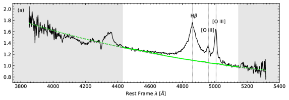
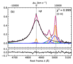
Figure 33: PKS 1937-101. Colours and lines as Figure 18.

This object shows a very faint Fe II emission, as is typical of A1 spectra. A UV spectrum from the MOJAVE/2CM atlas for this source is presented in Torrealba et al. (2012). It is also one of the strongest radio-loud sources we analyse in this work. Data from the Parkes 2.7 GHz Survey are shown in Savage et al. (1990). PKS 1937-101 is seen as a compact radio source after analysis of VLBI data (Lee et al. 2016).

Brinkmann & Siebert (1995) report PKS 1937-101 as one of the most distant objects detected with the ROSAT survey (Voges 1993).

A.17 PKS 2000-330

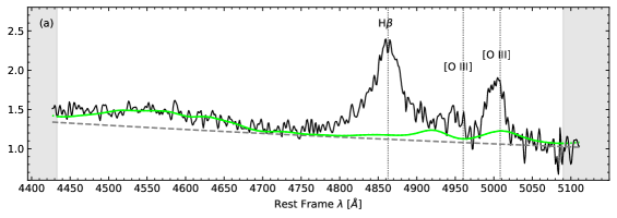
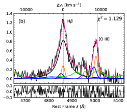
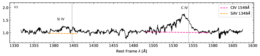
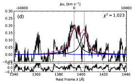
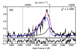
Figure 34: PKS 2000-330. Top panels: Same as Figure 23. (c) UV spectrum. Bottom panels: fittings for (d) Si IV$\lambda$1397 and (e) C IV$\lambda$1549Ṫhe UV spectrum was digitised from Barthel et al. (1990).

The UV spectrum used in the fittings was obtained through the digitisation of the spectrum from Barthel et al. (1990). However, since this spectrum presents a small wavelength range that does not account either for the 1900 Å blend or for He II$\lambda$1640, we analyse only the Si IV$\lambda$1397 and C IV$\lambda$1549 emission lines. A detailed comparison between this source and Q 1410+096 is performed in Deconto-Machado et al. (2022).

This quasar is the strongest radio-loud source from the present sample (Savage et al. 1990). The position of this source is not within the area covered by the FIRST catalogue.

A.18 SDSSJ210524.49+000407.3

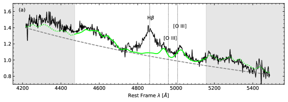
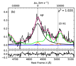
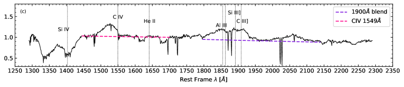
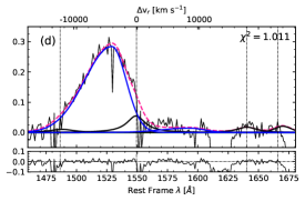
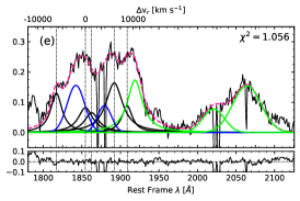
Figure 35: SDSSJ210524.49+000407.3. Top panels: Colours and lines as in Figure 18. (c) SDSS UV spectrum. Bottom panels: fittings for (d) C IV$\lambda$1549 and (e) the 1900 Å blend.

This source presents a $W$([O III]) $\approx$ 0.45Å. The low equivalent width makes it difficult to discern what corresponds to [O III]$\lambda\lambda$4959,5007 or to Fe II.

The UV region of this source is very unwieldy because of very broad absorption lines shortwards of C IV$\lambda 1459$. For the 1900 $\AA$ blend we present two different fittings, one including blueshifted components for Al III$\lambda$1860 and Si III]$\lambda 1892$ and another without these lines. The motivation here is that if we do not include blueshifted components then the BC of the lines present a displacement of $-1640$ km s^-1, which can be seen as an indicative of some outflowing gas.

A.19 SDSSJ210831.56-063022.5

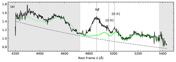
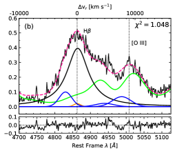
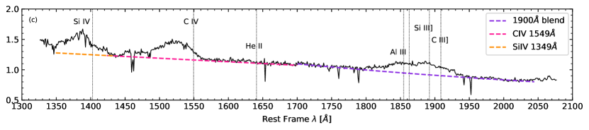
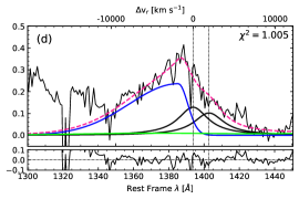
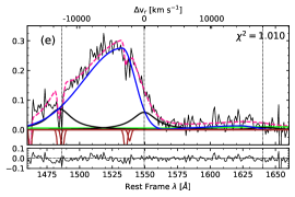
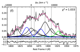
Figure 36: SDSSJ210831.56-063022.5. Same as Figure 23.

This is another case in which the Fe II contribution is estimated through the red side of the spectrum. It is difficult to set the [O III]$\lambda\lambda$4959,5007 NC at rest-frame since the region close to these lines is dominated by the Fe II multiplets. Differently from the other Pop. A3 of the sample (SDSSJ005700.18+143737.7 and SDSSJ210524.49+000407.3), for this quasar it was not possible to reach a good $\chi^{2}$ without including blueshifted components for Al III$\lambda$1860 and Si III]$\lambda$1892. SDSSJ210831.56-063022.5 is a source that presents one of the widest H$\beta$ BC of the sample. It could be that in this case the H$\beta$ BLUE component has been underestimated, since we do find strong blueward asymmetries in the three fitted UV profiles.

A.20 SDSSJ212329.46-005052.9

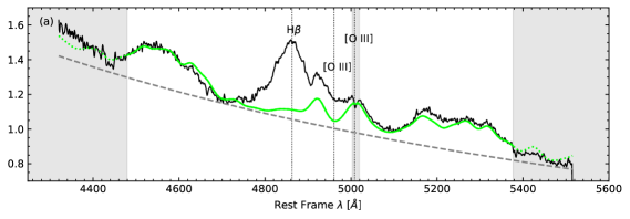
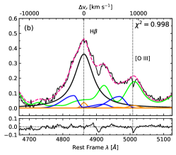
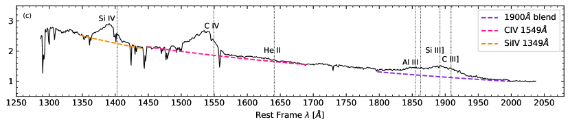
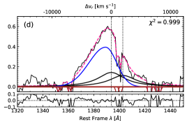
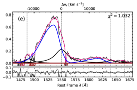
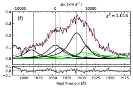
Figure 37: SDSSJ212329.46-005052.9. Same as Figure 23.

A.21 PKS 2126-15

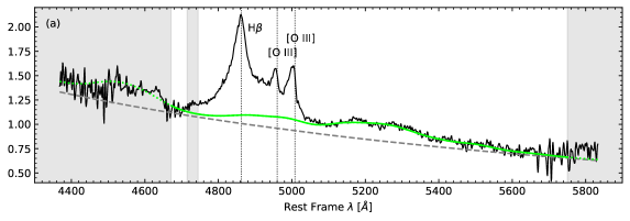
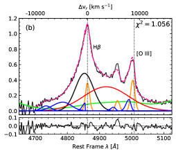
Figure 38: PKS 2126-15. Colours and lines as in Figure 18.

This object has been observed in the two runs. Since both observations can be used and present good S/N, we create a new spectrum by combining the two of them through the IRAF task scombine. The Fe II multiplets were fitted based on the shape seen in the red side of H$\beta$ due to the fact that the blue side of H$\beta$ is affected by noise and is almost at the border of the spectrum. In order to account for the [O III]$\lambda\lambda$4959,5007 contributions, it was necessary to include two blueshifted components, as can be seen in Fig. 38. Some UV spectra were found but they do not include the regions we are interested in.

PKS 2126-15 is also one of the four radio-loud quasars from the sample.

A.22 SDSSJ235808.54+012507.2

The spectrum of this source is of low S/N when compared with the other sources of the sample, which makes it difficult to find the correct intensity of the continuum. As a consequence, caution should be taken when considering the location of the continuum and the Fe II contribution especially in the blue part of the spectrum.