SuperRad: Modeling the black hole superradiance gravitational waveform

Abstract

Gravitational signatures of black hole superradiance are a unique probe of ultralight particles that are weakly-coupled to ordinary matter. The existence of an ultralight boson would lead spinning black holes with size comparable to the Compton wavelength of the boson to become superradiantly unstable to forming an oscillating cloud, spinning down the black hole, and radiating gravitational waves in the process. However, maximizing the chance of observing such signals or, in their absence, placing the strongest constraints on the existence of such particles, requires accurate theoretical predictions. In this work, we introduce a new gravitational waveform model, SuperRad, that models the dynamics, oscillation frequency, and gravitational wave signals of these clouds by combining numerical results in the relativistic regime with fits calibrated to analytical estimates, covering the entire parameter space of ultralight scalar and vector clouds with the lowest two azimuthal numbers ($m=1$ and 2). We present new calculations of the gravitational wave frequency evolution as the boson cloud dissipates, including using fully general-relativistic methods to quantify the error in more approximate treatments. Finally, as a first application, we assess the viability of conducting follow-up gravitational wave searches for ultralight vector clouds around massive black hole binary merger remnants. We show that LISA may be able to probe vector masses in the range from $1\times 10^{-16}$ eV to $6\times 10^{-16}$ eV using follow-up gravitational wave searches.

I Introduction

The advent of gravitational wave (GW) astronomy has brought a powerful tool to probe new physics in regimes that have been inaccessible to previous experiments. Illusive, weakly-coupled ultralight bosons beyond the Standard Model of particle physics have been conjectured to solve various problems in high energy physics and cosmology. However, terrestrial experiments require sufficiently strong coupling to the Standard Model for a direct detection. Therefore, gravitational signatures, which assume only that these ultralight particles gravitate, are ideal for efficiently probing the weak-coupling parameter space inaccessible to other observational efforts. Namely, black hole (BH) superradiance provides a purely gravitational mechanism through which ultralight bosonic particles extract rotational energy from spinning BHs with observable consequences.

Bosonic waves whose frequency satisfy the superradiance condition are amplified when scattering off a rotating BH Starobinsky (1973); Zel’Dovich (1971), extracting rotational energy in a type of Penrose process Penrose and Floyd (1971). If the underlying bosonic particle is massive, there is an instability associated with superradiance, leading to the formation of exponentially growing, oscillating bound states— superradiant clouds— around the BH. Assuming self-interactions and couplings to other matter are sufficiently weak, the instability saturates gravitationally as the BH loses energy and angular momentum, and is spun down. At this point, the system transitions from an exponentially growing phase to a phase characterized by quasi-monochromatic GW emission which causes the cloud to slowly dissipate. Therefore, the presence of the superradiant cloud leaves observational signatures in the BH spin distribution and the GW emission.

This observational window allows us to probe various well-motivated extensions to the Standard Model Arvanitaki et al. (2010). For scalar bosons, the QCD axion (solving the strong CP-problem), axion dark matter (solving the dark matter problem), and various quantum gravity motivated axion-like particles, are ultralight candidates capable of forming superradiant clouds Peccei and Quinn (1977); Weinberg (1978); Wilczek (1978); Arvanitaki et al. (2010); Essig et al. (2013); Hui et al. (2017); Marsh (2016). The dark photon is a viable candidate to make up a significant fraction of the dark matter, or could emerge in the low-energy limits of quantum gravity Goodsell et al. (2009); Jaeckel and Ringwald (2010). Ultralight spin-2 fields are a possible modification of general relativity Clifton et al. (2012). Hence, a wide variety of models could be constrained, or discovered via this observational window; addressing fundamental questions in particle physics, cosmology, and high energy physics.

To leverage the observational potential of ground- and space-based GW detectors, accurate predictions for the involved spin-down timescales, as well as GW frequency and amplitudes are required. Much effort has gone into determining these for scalar bosons Ternov et al. (1978); Zouros and Eardley (1979); Detweiler (1980); Dolan (2007); Arvanitaki and Dubovsky (2011); Yoshino and Kodama (2014); Arvanitaki et al. (2015, 2017); Brito et al. (2015a); Yoshino and Kodama (2015), vector bosons Rosa and Dolan (2012); Pani et al. (2012a, b); Cardoso et al. (2018); Baryakhtar et al. (2017); East (2017, 2018); Baumann et al. (2019a); Siemonsen and East (2020), and spin-2 fields Brito et al. (2013, 2020) (see Ref. Brito et al. (2015b) for a review). Scalar bosons exhibit the longest spin-down timescales, as well as weakest and longest GW signal after cloud formation. Vector bosons, on the other hand, are amplified more efficiently, leading to faster cloud growth rates and stronger, but hence shorter, GW emissions. In modified theories of gravity, massive spin-2 fields grow the fastest around BHs.

Using these results, various search strategies have been employed to constrain parts of the ultralight boson parameter space. Electromagnetic spin measurements of stellar mass and supermassive BHs McClintock et al. (2014); Miller and Miller (2014); Reynolds (2014) have been used to disfavor ultralight scalars Arvanitaki et al. (2015); Cardoso et al. (2018); Brito et al. (2017a); Stott (2020) and vectors Baryakhtar et al. (2017) in certain mass ranges. Similarly, measurements of spins of the constituents of inspiraling binary BHs Venumadhav et al. (2020); Abbott et al. (2019a, b) and BH population properties were used in Ref. Ng et al. (2021a, b); Payne et al. (2022) to exclude a small scalar mass range. Stochastic GW searches from a population of BH-cloud systems were used to constrain the scalar Brito et al. (2017a); Tsukada et al. (2019); Brito et al. (2017b) and vector Tsukada et al. (2021) masses, while various directed and blind continuous GW search techniques lead to constraints Sun et al. (2020); Palomba et al. (2019); D’Antonio et al. (2018); Isi et al. (2019); Zhu et al. (2020); Abbott et al. (2022a, b); Dergachev and Papa (2019). The presence of cloud around a constituent BH within a binary could also affect the inspiral dynamics, leaving observable signatures in the emitted GW waveform Hannuksela et al. (2019); Baumann et al. (2019a, 2022); Choudhary et al. (2021).

The methods used to determine the observable consequences of superradiance for a given BH of mass $M$, are classified by the their regime of validity for the dimensionless gravitational fine structure constant

$$\alpha\approx 0.075\left(\frac{M}{10\ M_{\odot}}\right)\left(\frac{\mathcal{M}}{10^{-12}\ \text{eV}}\right),$$ (1)

where $\mathcal{M}$ is the mass of the ultralight particle. Analytic techniques are most accurate for $\alpha\ll 1$, the regime where the boson cloud is farther away from the BH and can be treated non-relativistically. However, numerical approaches are required for systems with $\alpha\sim\mathcal{O}(1)$, where the cloud sits close to the BH, and relativistic effects are import. Analytic estimates have been pushed to high orders in an expansion around small $\alpha$, while numerical techniques have been refined to include large parts of the parameter space. Despite this progress, and the significant impact of gravitational probes, most gravitational and electromagnetic wave search campaigns for signatures of BH superradiance have employed lower-order, potentially inaccurate, predictions, leaving the most favorable parts of the parameter space unexplored.

Here, we introduce SuperRad, an open source BH superradiance waveform model incorporating state-of-the-art theoretical predictions for BH spin-down and GW observables across the entire relevant parameter space in a simple, ready-to-use python package. A primary goal is to provide a tool to efficiently and accurately interpret GW search results of current and future ground- and space-based GW observatories. As part of this work, we present new calculations of the frequency evolution of the boson cloud oscillations and attendant GWs due to the changing mass of the boson cloud. We compare the analytic frequency evolution in the non-relativistic limit to both approximate quasi-relativistic calculations, as well as fully general-relativistic ones, to determine their accuracy in the relativistic regime.

As a first application, we use SuperRad to show that the Laser Interferometer Space Antenna (LISA) should in principle be able to probe ultralight boson masses from $1\times 10^{-16}$ eV to $6\times 10^{-16}$ eV by performing follow-up searches for GWs from boson clouds arising around the remnants of massive BH binary mergers. Such follow-up searches have been previously discussed in the context of stellar mass BH mergers Ghosh et al. (2019); Isi et al. (2019); Chan and Hannuksela (2022), and are especially promising because the observation of the binary BH merger waveform gives definitive information on the properties of the remnant BH, allowing one to place constraints in the absence of a signal without further assumptions. By contrast, other search methods outlined above rely on further assumptions and are subject to various uncertainties: electromagnetic spin measurements are contingent on astrophysical uncertainties and may be invalidated by weak couplings of the ultralight boson to the Standard Model Siemonsen et al. (2022), spin measurements of constitutents of inspiraling binary BHs have large statistical uncertainties, and constraints based on blind continuous waves and stochastic gravitational wave background searches rely on BH population assumptions.

We begin in Sec. II by providing a broad overview over the expected GW signals from BH superradiance of scalar and vector clouds. In Sec. III, we discuss in detail how SuperRad determines the cloud’s oscillation frequency and the superradiance instability timescales. Furthermore, we analyze the frequency shift due to the finite self-gravity of the cloud around the BH in Sec. IV using Newtonian, quasi-relativistic, and fully relativistic approaches. The GW amplitude and waveform is discussed in Sec. V. Following this, we outline the linear evolution of the cloud as well as the accompanying GW signature in Sec. VI, and close with the application of SuperRad to analyze the prospects of follow-up searches with LISA in Sec. VII. We use $G=c=1$ units throughout.

II Overview and Example

We begin with an example to illustrate the expected GW signal from superradiant clouds, and give an overview of the different effects that go into calculating it. We consider parameters consistent with the remnant from a GW150914-like binary BH merger. In particular, we consider a BH with mass $M=62\ M_{\odot}$ and dimensionless spin $a_{*}=0.67$ at a distance of 410 Mpc Abbott et al. (2016) and determine the resulting GW signal if there were an ultralight boson—scalar or vector—with mass $\mathcal{M}=3.6\times 10^{-13}$ eV (hence $\alpha\approx 0.17$). For simplicity, here we assume the angular momentum points in the direction of the observer—hence both GW polarizations are equal—and ignore redshift effects. The GW strain and frequency calculated with SuperRad for both the scalar boson case and the vector case are shown in Fig. 1.

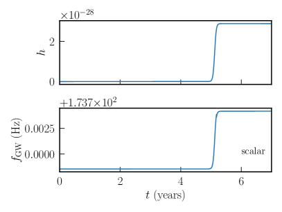
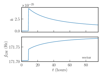
Figure 1: The GW strain $h$ and frequency $f_{\rm GW}$ as a function of time for a BH with $M=62\ M_{\odot}$ and $a_{*}=0.67$ at a distance of 410 Mpc subject to the superradiant instability of a boson with mass $3.6\times 10^{-13}$ eV. The top set of panels shows the scalar boson case, while the bottom set shows the vector case. Note the difference in timescales shown, since in the scalar (vector) case the cloud grows on timescales of $\sim 5$ years (9 hours) and decays through GW radiation on timescales of $\sim 9000$ years (1 day). Time is measured since the BH was formed, assuming the cloud started as a single boson.

There are a number of different parts that go into these calculations. First, one determines the superradiant instability timescale by solving for the fastest growing mode of the massive scalar or vector equations of motion on the BH spacetime as described in Sec. III. This gives the timescale over which the boson cloud mass, and hence the GW amplitude, grows exponentially in time. From Fig. 1, it can be seen that the $e$-folding time of the cloud mass (half the $e$-folding time of the field $\tau_{I}$) is much slower for the scalar case ($\tau_{I}/2\sim 10$ days) compared to the vector case ($\tau_{I}/2\sim 3$ minutes). Taking into account the resulting decrease in the mass and spin of the BH as the boson cloud grows, as described in Sec. VI, the instability timescale becomes longer and longer as the horizon frequency of the BH approaches the oscillation frequency of the cloud. As the instability saturates, and the cloud mass reaches its maximum value, the dissipation of the cloud through gravitational radiation becomes dominant, leading to a slow decrease in cloud mass. The rate at which energy is lost through gravitational radiation $P_{\rm GW}$, as well as the two strain polarizations $h_{+}$ and $h_{\times}$, are calculated by solving for linearized metric perturbations on the BH spacetime, sourced by the oscillating cloud solution, as described in Sec. V. As can be seen in Fig. 1, in the scalar case the decay of GW amplitude is negligible on any reasonable observing timescale, taking on the order of $10^{4}$ years, while in the vector case, the cloud mass and GW amplitude decrease on timescales of days.

The gravitational frequency shown in Fig. 1 exhibits an increase or “chirp” in frequency, first as the BH loses mass and the cloud grows exponentially, and then more slowly as the boson cloud dissipates. Calculating this frequency shift requires accounting for the self-gravity of the boson cloud, which slightly red-shifts the oscillation frequency of the cloud, and hence the gravitational waves (which have twice the frequency of the cloud oscillations), as described in Sec. IV. Though the change in frequency is small, because the GW signal persists for many cycles, this is still an important effect.

III Cloud properties

In this section, we outline the superradiant cloud properties relevant for observational signatures such as BH spin-down or GW emission. This includes a brief discussion of how estimates for the superradiant instability timescale $\tau_{I}$ and the emitted GW frequency $f_{\rm GW}$ are obtained for different values of the BH mass, spin, and the gravitational fine structure constant $\alpha$. We defer the analysis of the dependency of the cloud frequency on cloud mass, and the cloud dynamics to Secs. IV and VI, respectively. SuperRad combines analytic and numerical predictions, valid for $\alpha\ll 1$ and $\alpha\sim\mathcal{O}(1)$, and utilizes numerically calibrated higher-order expansions to interpolate between the two regimes.

In most of the following calculations, we assume a fixed Kerr BH spacetime $g_{\mu\nu}$, and consider scalar and vector bosonic fields, as well as linear metric (GW) perturbations on this background. The exception to this is the calculation of the frequency shift due to the self-gravity of the boson-cloud. We will discuss the validity of this assumption further in Secs.V.2 and IV. Furthermore, we neglect field self-interactions and non-minimal couplings to the Standard Model throughout, which have been investigated in Refs. Yoshino and Kodama (2012); Fukuda and Nakayama (2020); Baryakhtar et al. (2021); East (2022); East and Huang (2022); Omiya et al. (2022). Depending on the coupling strength, these can alter the superradiance dynamics. However, here we assume that we are in the weak coupling limit, which reduces to the purely gravitational case. Therefore, the relevant field equations to solve in order to obtain the desired observables are the scalar and vector massive wave equations on the spacetime $g_{\mu\nu}$, which are given by

$$(\square_{g}-\mu_{S}^{2})\Phi=0, \nabla_{\mu}F^{\mu\nu}=\mu^{2}_{V}A^{\nu},$$ (2)

where $\mathcal{M}_{S}=\hbar\mu_{S}$ and $\mathcal{M}_{V}=\hbar\mu_{V}$ are the scalar and vector boson masses, respectively. Due to various symmetries of the Kerr spacetime, solutions to the field equations (2) can be written in the form

$$A_{\mu},\Phi\sim e^{-i(\omega t-m\varphi)},$$ (3)

where we introduced the azimuthal mode number $m$ and complex frequency $\omega$. Here, and in the following, we refer to the Boyer-Lindquist time, radius, polar and azimuthal coordinate as $t$, $r$, $\theta$, and $\varphi$. Without loss of generality, we assume the azimuthal index to satisfy $m\geq 0$ throughout. Lastly, we label all quantities defined both for scalar and vector fields with $\sigma\in\{S,V\}$. The fields $A_{\mu}$ and $\Phi$ are susceptible to the superradiance instability, if the superradiance condition

$$0<\omega_{R}<m\Omega_{H},$$ (4)

is satisfied, where $\Omega_{H}$ is the horizon frequency of the BH. In the ansatz (3), the frequency $\omega=\omega_{R}+i\omega_{I}$ encodes both the oscillation frequency of the cloud, which is half of the characteristic GW frequency $f_{\rm GW}=2\omega_{R}/(2\pi)$ (up to self-gravity corrections), and the instability growth timescale $\tau_{I}=1/\omega_{I}$. For fixed mode number $m_{\sigma}$, these observables (in units of $M$) depend only on $\alpha$ and spin $a_{*}$, i.e., $\omega(\alpha,a_{*})$.

In what follows, we begin by outlining SuperRad’s coverage of the $(\alpha,a_{*})$ parameter space in Sec. III.1, and then we illustrate how analytic and numerical results are used to calibrate SuperRad in the intermediate regime in Secs. III.2 and III.3.

III.1 Parameter space

In Figure 2, we show the parameter space for the $m_{V}=1$ massive vector as an illustrative example. For a given quantity $q(\alpha,a_{*})\in\{\omega_{R},\omega_{I},\partial_{t}\omega_{R}\}$ (in units of $M$), we numerically calculate its value in the relativistic regime, but for computational reasons, do not extend our calculations deep into the small-$\alpha$ regime. We want to match on to analytic results $q_{N}$ that are valid only in the Newtonian limit, when $\alpha\ll 1$. We do this by dividing the parameter space in $(\alpha,a_{*})$ into two regions. In the relativistic regime, labelled $\mathcal{D}_{\rm int}$, we merely interpolate between the numerically computed points using the interpolation polynomial $I_{R}(\alpha,a_{*})$. In the regime where $\alpha$ is smaller, labelled $\mathcal{D}_{\rm fit}$, we use a subset of the numerical results in $\mathcal{D}_{\rm int}$ (corresponding to the red points in Fig. 2) and fit the difference between these results and the analytic ones in a way that is guaranteed to recover the latter at sufficiently small $\alpha$. That is, we let

$$q(\alpha,a_{*})=\begin{cases}q_{N}(\alpha,a_{*})+g(\alpha,a_{*}),&(\alpha,a_{*})\in\mathcal{D}_{\rm fit},\\ I_{R}(\alpha,a_{*}),&(\alpha,a_{*})\in\mathcal{D}_{\rm int}.\end{cases}$$ (5)

where $g$ is a fitting function chosen to give $q_{N}(\alpha,a_{*})+g(\alpha,a_{*})\to q_{N}(\alpha,a_{*})$ as $\alpha\to 0$. The specific choices of $\mathcal{D}_{\rm fit}$ and $\mathcal{D}_{\rm int}$ depend on the field and azimuthal mode in question, and are determined by the accuracy of the underlying methods (these are defined in App. C). Note also that we are only interested in the part of the parameter space where $\omega_{R}\leq m_{\sigma}\Omega_{H}$, since outside this range the cloud will be exponentially decaying through absorption by the BH.

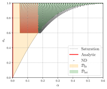
Figure 2: The parameter space of the superradiant $m_{V}=1$ vector mode. It is made up of relativistic regime $\mathcal{D}_{\rm int}$, where SuperRad employs interpolation functions based on the numerical data (labelled ND) to determine a given quantity $q(\alpha,a_{*})$ and a lower $\alpha$ region $\mathcal{D}_{\rm fit}$, where numerical calibration is necessary to augment the expressions valid in the Newtonian limit $\alpha\to 0$ (indicated by a red line). For illustration purposes, we show only $40^{2}$ of the $320^{2}$ data points used in SuperRad. The gray dashed line marks the saturation point of the superradiance instability, i.e., $\omega_{R}=\Omega_{H}(a_{*})$. In this case, the red data points are used for calibration in $\mathcal{D}_{\rm fit}$.

In the relativistic part of the parameter space $\mathcal{D}_{\rm int}$, a set of $320^{2}$ waveforms are generated for the azimuthal modes $m_{\sigma}=1$ and $2$, and for both the scalar and the vector case. The grid of waveforms is uniformly spaced in the coordinates $(y,a_{*})$, with $y\in[0,1]$, defined by

$$y=\frac{\alpha-\alpha_{0}}{\alpha_{1}-\alpha_{0}},$$ (6)

where $\alpha_{0}^{m_{\sigma}=1}=0.05$ and $\alpha_{0}^{m_{\sigma}=2}=0.25$, while $\alpha_{1}$ is the solution to

$$\beta\alpha_{1}\left[1-\frac{\alpha_{1}^{2}}{2n_{\sigma}^{2}}\right]=m_{\sigma}M\Omega_{H}(a_{*}),$$ (7)

with $\beta=0.9$, and $n_{\sigma}$ is the cloud’s principle number defined below in (10). This choice of $\alpha_{1}$ is made so as to guarantee that $y=1$ lies outside the superradiant regime, and thus that the saturated state $\omega_{R}=m_{\sigma}\Omega_{H}$ lies within the grid. The boundary $y=1$ corresponds to the large-$\alpha$ boundary of the numerical data in Figure 2, beyond the superradiant saturation.

III.2 Oscillation frequencies

The real part of the superradiantly unstable field’s frequency determines the cloud’s oscillation about the BH

$$A_{\mu},\Phi\sim\cos(\omega_{R}t),$$ (8)

and also sets the characteristic GW frequency $f_{\rm GW}=\omega_{R}/\pi$ (up to self-gravity corrections). Because of the BH’s gravitational potential, a bound massive particle has a frequency $\omega_{R}<\mu$. Expanding (2) to leading order in $\alpha$ yields a Schrödinger-type equation with potential $U\sim\alpha/r$, at a radius $r$ away from the BH. In this regime, the solutions are simple hydrogen-like bound states for scalar and vector fields Detweiler (1980); Pani et al. (2012b). The scalar states are characterized by their angular momentum quantum number $\ell_{S}$, as well as azimuthal mode number $-\ell_{S}\leq m_{S}\leq\ell_{S}$ and radial node number $\hat{n}_{S}\geq 0$, while the vector states are identified by an analogous definition of radial node number $\hat{n}_{V}\geq 0$, angular momentum number $\ell_{V}$ and azimuthal index $m_{V}$, in addition to the polarization state $\hat{S}\in\{-1,0,1\}$. With this, the oscillation frequencies of the scalar and vector clouds are, in the non-relativistic limit,

$$\omega_{R}=\mu\left(1-\frac{\alpha^{2}}{2n^{2}_{\sigma}}+C_{\sigma}[\alpha]\right),$$ (9)

where $C_{\sigma}[\alpha]$ includes higher order corrections. In particular, we include terms of up to $\mathcal{O}(\alpha^{5})$, obtained by keeping sub-leading contributions in $\alpha$ when solving (2) Baumann et al. (2019a), with the full expressions for $C_{\sigma}$ given in appendix B [in particular (41) and (48)]. The state label $n_{\sigma}$, depends on the intrinsic spin of the field and is given by

$$n_{S}=\ell_{S}+1+\hat{n}_{S}, n_{V}=m_{V}+\hat{n}_{V}+\hat{S}+1.$$ (10)

Notice, in the case of the scalar field, we follow the conventions of Ref. Baumann et al. (2019a), while in the vector case, we follow Ref. Dolan (2018). In the language of the previous section, the expressions (9) are the Newtonian estimates $q_{N}(\alpha,a_{*})$.

We numerically estimate $\omega_{R}$ using the methods discussed in appendix B, without assuming an expansion in small $\alpha$. These estimates are calculated for $m_{\sigma}\in\{1,2\}$ for both scalar and vector fields. Here, we simply summarize that our numerical methods are more accurate and precise than the analytic estimates everywhere in $\mathcal{D}_{\rm int}$. The waveform model provides accurate values for $\omega_{R}$ in $\mathcal{D}_{\rm fit}$ using a fit to the numerical results. We perform this fit using the ansatz

$$\frac{\omega_{R}}{\mu}-1+\frac{\alpha^{2}}{2n^{2}_{\sigma}}-C_{\sigma}[\alpha]=\sum_{q,p}\alpha^{p}\hat{a}_{p,q}(1-a_{*}^{2})^{q/2},$$ (11)

with appropriately chosen ranges for $p$ and $q$, to the numerical data in a subset of $\mathcal{D}_{\rm int}$ (see appendix C for details). The right-hand side of (11) corresponds to $g(\alpha,a_{*})$, defined in the previous section. This ansatz explicitly assumes the analytic estimates in the $\alpha\ll 1$ regime. Within SuperRad, we combine all three of these ingredients as described in (5) to determine $\omega_{R}$ in the parameter space. Therefore, we ensure that SuperRad provides the most accurate and precise estimate for frequencies of a given superradiant bosonic field around a fixed Kerr BH background across the entire parameter space. The correction of these frequency estimates due to the self-gravity of the superradiant cloud is discussed in Sec. IV.

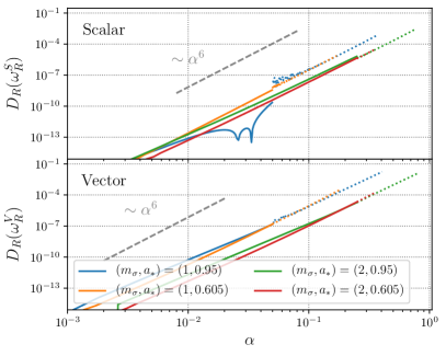
Figure 3: The relative difference $D_{R}$, between the prediction for $\omega_{R}$ provided by SuperRad, and purely analytical non-relativistic estimates given in (9) together with (41) and (48). Dotted lines indicate the $\mathcal{D}_{\rm int}$ region in SuperRad. We focus on a few representative cases.

In Figure 3, we compare the available analytic estimates, given in (9) [together with (41) and (48)], with those provided by SuperRad. As expected, the relative difference between the analytic estimates and SuperRad’s decay as $\sim\alpha^{6}$ [the order of the leading-in-$\alpha$ unknown coefficient in the expansion of (9)] in the Newtonian regime. For large spins $a_{*}$ and large $\alpha$, i.e., in the relativistic regime, the analytic estimates have relative errors up to $D_{R}(\omega_{R})\lesssim 10^{-2}$. In comparison to the vector results, the analytic estimates for $\omega_{R}^{S}$ are more accurate in the most relativistic regime.

III.3 Instability timescales

The imaginary part of the frequency $\omega_{I}$ sets the superradiant instability timescale $\tau_{I}=1/\omega_{I}$ of the bosonic cloud,

$$A_{\mu},\Phi\sim e^{\omega_{I}t}.$$ (12)

In the non-relativistic limit $\alpha\to 0$, the cloud sits far away from the BH and the flux across the horizon, and hence the instability growth rate, tends towards zero. For small, but non-zero $\alpha$, the rates scale with a characteristic power $\kappa$, i.e., $\omega_{I}M\sim\alpha^{\kappa}$. This scaling depends on the type of field (scalar or vector) and the mode considered. Furthermore, at saturation, i.e., when $\omega_{R}=m_{\sigma}\Omega_{H}$, the ultralight particles cease extracting rotational energy from the BH, such that the growth rate vanishes. Combining these two limits, the general behavior of the instability growth rates for both the scalar and the vector cases is

$$\omega_{I}M=\alpha^{\kappa}(\omega_{R}-m_{\sigma}\Omega_{H})2r_{+}G_{\sigma}(a_{*},\alpha).$$ (13)

Here, $G_{\sigma}(a_{*},\alpha)$ is a function of the BH spin, as well as $\alpha$, and determines the leading order and sub-dominant-in-$\alpha$ contributions to $\omega_{I}$. The scaling power $\kappa$, for scalar and vector fields are Detweiler (1980); Pani et al. (2012a)

$$\kappa_{S}=4m_{S}+5, \kappa_{V}=4m_{V}+2\hat{S}+5,$$ (14)

for the fastest growing configurations, and depend on the azimuthal index $m_{\sigma}$ and the vector polarization state $\hat{S}$. The leading order contributions in the scalar case Detweiler (1980) and the vector case Rosa and Dolan (2012); Pani et al. (2012b); Baryakhtar et al. (2017); Baumann et al. (2019a) to $G_{\sigma}(a_{*},\alpha)$ that we use are given in Appendix B [in particular (43) and (51), respectively]. These are Newtonian estimates that we use [$q_{N}(\alpha,a_{*})$ in the language of Sec. III.1] for the imaginary frequency.

Similarly to the previous section, we utilize numerical techniques to obtain accurate predictions for $\omega_{I}$ in the relativistic regime $\mathcal{D}_{\rm int}$ of the parameter space. The methods and their accuracy are outlined in Appendix B. Here, we simply note again that the numerical predictions are more accurate than the analytic Newtonian expressions everywhere in $\mathcal{D}_{\rm int}$. Similar to the real part of the cloud’s frequency, the analytic results obtained in the Newtonian limit are connected with the numerical estimates in the $\alpha\sim 1$ regime by fitting the ansatz

$$\begin{aligned} &\frac{\omega_{I}M\alpha^{-\kappa}G^{-1}_{\sigma}(a_{*},\alpha)}{2r_{+}(\omega_{R}-m_{\sigma}\Omega_{H})}-1\\ &\qquad=\sum_{p,q}\alpha^{p}\left[\hat{b}_{p,q}a_{*}^{q+1}+\hat{c}_{p,q}(1-a_{*}^{2})^{q/2}\right],\end{aligned}$$ (15)

with appropriately chosen ranges for $p$ and $q$, to the numerical data obtained in $\mathcal{D}_{\rm int}$ (see Appendix C for details). The right-hand-side of (15) serves as $g(\alpha,a_{*})$ in the construction (5) for $\omega_{I}$. Analogously to the oscillation frequency, with this construction we ensure SuperRad provides the most accurate and precise estimates for the superradiance growth rate $\omega_{I}$ everywhere in the cloud’s parameter space.

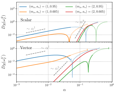
Figure 4: The relative difference $D_{R}$ between the prediction for $\omega_{I}$ provided by SuperRad, and purely analytical non-relativistic estimates given in (13) together with (43) and (51). Dashed lines indicate the $\mathcal{D}_{\rm int}$ region in SuperRad. We show the same representative cases as in Figure 3.

In Figure 4, we illustrate the relative differences between the analytic estimates using only (13) together with (43) and (51), and the estimates provided by SuperRad. In the Newtonian regime, the relative difference approaches zero, while in the relativistic regime, the relative error in the analytic estimates becomes $D_{R}(\omega_{I})\sim\mathcal{O}(1)$ in both the scalar and the vector cases. Hence, using non-relativistic analytic estimates in the relativistic regime can lead to large systematic uncertainties in the instability rate. We indicate the leading-in-$\alpha$ scaling of the difference for each $m_{\sigma}$. An $\sim\alpha^{1}$-scaling is expected in principle for both $m_{\sigma}=1$ and $m_{\sigma}=2$, however, due to our choices of $p$ and $q$ in (15) (see also Appendix C), the leading power is $>1$ for $\alpha\ll 1$ in the $m_{\sigma}=2$ case. For $\alpha\gtrsim 0.1$, the scaling decreases to the expected $\sim\alpha^{1}$.

IV Frequency shift

So far, we have considered calculations that assume the bosonic field can be treated as a test field on a Kerr background. Even for cases where the boson cloud mass reaches $M_{c}\sim 0.1M$, treating the spacetime as Kerr, with quasi-adiabtically changing parameters, gives a good approximation to the nonlinear treatment East and Pretorius (2017); East (2018). However, in this section, we address the effect of the self-gravity of the cloud, focusing in particular on how it causes the characteristic increase in frequency of the cloud oscillation, and hence the frequency of the emitted GW radiation. Though the cloud-mass induced shift in the frequency is small, it will change as the cloud slowly dissipates through gravitational radiation, affecting how long the GW signal can be coherently integrated without taking this effect into account. Quantitatively estimating the contribution to the frequency from the finite cloud mass

$$\Delta\omega(M_{c})=\omega(M_{c})-\omega(M_{c}=0)$$ (16)

(which we will assume to be real) is the subject of this section. We employ a Newtonian approach, recovering and extending known results in the literature. We then compare these results in the scalar case to a fully nonlinear approach using synchronized complex fields around BHs.

IV.1 Newtonian approach

The Newtonian approach, utilized to estimate the cloud mass correction to the frequency in Refs. Baryakhtar et al. (2017); Isi et al. (2019); Baryakhtar et al. (2021), exploits the fact that in the non-relativistic limit, the energy density $\rho$ is spread out over large scales away from the BH, minimizing curvature effects. In this limit, the cloud itself sources a Newtonian gravitational potential $\Psi$, which follows the Poisson equation:

$$\Delta_{\text{flat}}\Psi=4\pi\rho, \Psi(\textbf{r})=-\int d^{3}\textbf{r}^{\prime}\frac{\rho(\textbf{r}^{\prime})}{|\textbf{r}-\textbf{r}^{\prime}|}.$$ (17)

Here, the coordinates r can be identified with spatial slices of Kerr, where gauge ambiguities disappear in the $\alpha\ll 1$ limit. Furthermore, while one might choose $d^{3}\textbf{r}^{\prime}=\sqrt{\gamma}d^{3}x^{\prime}$, with the determinant of the metric of a spatial slice of Kerr, a priori this is not more consistent than simply setting $\gamma\rightarrow\gamma_{\text{flat}}$, which is our choice. In this weak-field limit, the scalar wave equation (2) is given by

$$(\omega-\mu_{S})\Phi(\textbf{r})\approx\left(-\frac{\nabla^{2}}{2\mu_{S}}-\frac{\mu_{S}M}{r}+\mu_{S}\Psi\right)\Phi(\textbf{r})\ ,$$ (18)

with $r=|\textbf{r}|$. Taking the usual approximation that the shift in frequency at leading order in $\alpha$ is given by evaluating the perturbed operator on the unperturbed eigenfunction, the self-gravity of a cloud with mass $M_{c}=\int d^{3}\textbf{r}\rho(\textbf{r})$ contributes a shift in frequency of

$$\Delta\omega\frac{M_{c}}{\mu} \approx\int d^{3}\textbf{r}\rho\Psi$$

$$=2\int d^{3}\textbf{r}\int_{|\textbf{r}^{\prime}|<|\textbf{r}|}d^{3}\textbf{r}^{\prime}\frac{\rho(\textbf{r})\rho(\textbf{r}^{\prime})}{|\textbf{r}-\textbf{r}^{\prime}|}=2W.$$ (19)

We used the non-relativistic approximation that $\rho\approx\mu^{2}|\phi|^{2}$, and in the last line introduced the total potential energy $W$ in the cloud. We note that this factor of $2$ (from restricting the inner integral) is missing from some references Baryakhtar et al. (2017); Isi et al. (2019), but included in Ref. Baryakhtar et al. (2021). An equivalent derivation gives the same expression (19) in the vector case as well.

We can further simplify the frequency shift calculation by considering a low multipole approximation. The denominator of (19) can be expanded in terms of spherical harmonics $Y_{\ell m}(\Omega)$, where $(\Omega)=(\theta,\varphi)$ describes the angular dependence, as

$$\frac{1}{|\textbf{r}-\textbf{r}^{\prime}|}=\sum_{\ell=0}^{\infty}\sum_{m=-\ell}^{\ell}\frac{r^{\prime\ell}}{r^{\ell+1}}\frac{4\pi}{2\ell+1}Y_{\ell m}(\Omega)\bar{Y}_{\ell m}(\Omega^{\prime}),$$ (20)

assuming $|\textbf{r}^{\prime}|<|\textbf{r}|$. If we keep only the monopolar, i.e., the $\ell=0$, component of the density, which we can write in terms of the radial mass function $m_{c}(r)=\int d\Omega^{\prime}\int_{0}^{r}dr^{\prime}r^{\prime 2}\rho(\textbf{r}^{\prime})$, then (19) simplifies to

$$\Delta\omega=-\frac{2\mu}{M_{c}}\int d^{3}\textbf{r}\frac{m_{c}(|\textbf{r}|)\rho(\textbf{r})}{|\textbf{r}|}.$$ (21)

In general, there are non-vanishing higher order multipoles due to the non-trivial azimuthal and polar dependencies of the cloud’s energy densities that are neglected above. However, for the $m_{S}=1$, the error in the calculation of $W$ associated with making this monopole approximation, as opposed to considering higher multipole corrections, is $\approx 2\%$ at leading order in $\alpha$ . In the $m_{V}=1$ case, all higher-order multipolar contributions are sub-leading in $\alpha$, since the Newtonian energy density is spherically symmetric. While the cloud states with larger azimuthal number have strong polar dependencies, the corrections from high-order multipoles is moderate. For the $m_{V}=2$ state, the quadrupolar contribution is $\approx 2\%$ of the monopolar piece, at leading order in $\alpha$. The frequency shift $\Delta\omega$ is then calculated for different modes of the non-relativistic solutions to (18) for scalar clouds, and for corresponding non-relativistic vector cloud solutions. Expressions for $\Delta\omega$, valid for any azimuthal index $m_{\sigma}$, as well as a table listing the first few values, are given in (52) and in Table 1, respectively.

IV.2 Quasi-relativistic

These analytic expressions (52) are accurate in the Newtonian limit, i.e., $\alpha\ll 1$. Here, we extend the validity to the $\alpha\sim\mathcal{O}(1)$ regime, with the caveat that a more accurate nonlinear treatment, discussed in the next section, is ultimately necessary. Within SuperRad, we compute the frequency shift in the relativistic regime $\mathcal{D}_{\rm int}$ in a quasi-relativistic approximation, as in Ref. Siemonsen and East (2020). We take the relativistic field configurations (derived in Appendix B) in Boyer-Lindquist coordinates and use them to compute the energy density $\rho$, which we then use to compute the frequency shift $\Delta\omega$ using the monopolar Newtonian expression (21). This approach explicitly assumes a linear dependence of the frequency shift on the cloud mass: $\Delta\omega\sim M_{c}$. Given these quasi-relativistic results in the relativistic regime of the parameter space, we follow the approach taken in Secs. III.2 and III.3, to calibrate a fit that assumes the analytic expressions (52) against the quasi-relativistic results in $\mathcal{D}_{\rm int}$. The fit ansatz is

$$\frac{M^{2}\Delta\omega}{-\alpha^{3}M_{c}}+F_{\sigma}=\sum_{p\geq 1}\alpha^{p}\hat{d}^{\sigma}_{p},$$ (22)

where $F_{\sigma}$ contains the leading-in-$\alpha$ contribution, computed above and explicitly given in Appendix D.

As a figure of merit for comparing how relevant this will be in GW observations of boson clouds, we can calculate the extra accumulated phase shift due to the frequency drift, using that $\omega_{\rm GW}=2\omega_{R}$,

$$\Delta\phi_{\rm GW}=2\int_{t_{\rm max}}^{t_{\rm max}+\tau}\left[\omega_{R}(t)-\omega_{R}(t_{\rm max})\right]dt,$$ (23)

where $t_{\rm max}$ is the time the cloud mass is at its maximum. We show this for the scalar and vector case in Fig. 5, taking the total time $\tau=\min(\tau_{\rm GW},1\text{yr})$ to be either the characteristic time over which the GW signal decays $\tau_{\rm GW}$, or one year, when $\tau_{\rm GW}>1$ yr (assuming a $50\ M_{\odot}$ BH). From the figure, we can see that $\Delta\phi_{\rm GW}\gg 1$ across the parameter space, except for the scalar case when $\alpha\lesssim 0.1$. Thus, properly accounting for this frequency shift is important to be able to coherently integrate the GW signal. The diverging behavior of the $\tau=\tau_{\rm GW}$ curves in Fig. 5 at low $\alpha$ is due to the steeper $\alpha$-scaling of the GW timescales compared with the frequency shift’s scaling.

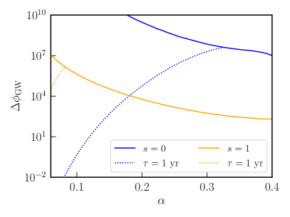
Figure 5: The additional accumulated GW phase $\Delta\phi_{\rm GW}$ due to the increase in frequency as the boson cloud mass decreases [defined in (23)] for scalar (blue curves) and vector (orange curves) bosons. This phase is calculated beginning from when the cloud mass is maximum for a duration of $\tau_{\rm GW}$ (solid curves) and for one year (when $\tau_{\rm GW}>1$ yr; dotted curves). We assume a BH with $M=50\ M_{\odot}$ and $a_{*}=0.99$.

IV.3 Comparison to fully relativistic approach

To gauge the error in the quasi-relativistic frequency shifts described above, we compare them to numerically constructed, fully relativistic solutions. Following Herdeiro & Radu Herdeiro and Radu (2015), we construct stationary and axisymmetric spacetime solutions to the full Einstein-Klein-Gordon field equations consisting of a massive complex scalar field cloud with $\Phi\sim e^{im_{S}\phi-i\omega_{R}t}$ around a BH, satisfying the synchronization condition $\omega_{R}=m_{S}\Omega_{H}$. These can be thought of as oscillation (or, equivalently, azimuthal angle) averaged versions of the scalar cloud solutions. By calculating how the frequency of the solution changes with $M_{c}$ at fixed $M$ and $\alpha$, we can obtain a fully-relativistic estimate for the frequency shift $\Delta\omega$. The frequency shift is the part of the real frequency that is dependent on the boson cloud mass, $\omega(M_{c})=\omega(M_{c}=0)+\Delta\omega(M_{c})$. For the values of cloud mass relevant to superradiance, $\Delta\omega$ is, to a good approximation linear in $M_{c}$, as expected from the non-relativistic results above. Therefore, here we compute a numerical estimate of $\partial\omega/\partial M_{c}$ at $M_{c}=0$ and fixed $\alpha$ (which is $\approx\Delta\omega/M_{c}$, to within $\sim 1\%$ for $M_{c}<0.04M$). In Fig. 6, we show how this compares, for $m_{S}=1$, to the non-relativistic and quasi-relativistic results for the frequency shift. From there it can be seen that the quasi-relativistic estimate used by SuperRad is slightly more accurate than the non-relativistic expressions, but still noticeably underestimates the frequency decrease, by $\approx 32\%$, for $\alpha=0.4$. For small $\alpha$, all three calculations give similar results, as expected. In particular, for $\alpha<0.15$, the difference in the quasi- versus the fully relativistic calculation is $<7\%$.

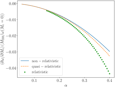
Figure 6: A comparison of different approximations of the frequency shift due to the boson cloud’s self-gravity for a scalar field with $m_{S}=1$. We compare the non-relativistic (see Sec. IV.1) and quasi-relativistic (see Sec. IV.2) approximations to the (leading order in $M_{c}$ part) fully relativistic (labelled “relativistic”) relative frequency shift. In particular, we show, for fixed $\alpha$, $(\partial\omega/\partial M_{c})(M_{c}=0)\approx\Delta\omega/M_{c}$, where the equality is exact for the non-relativistic and quasi-relativistic approximations.

We plan to include the fully relativistic frequency corrections in a future version of SuperRad, and we defer details on constructing the BH-complex boson cloud solutions, as well as the massive vector case (where we expect comparable, if somewhat larger, relativistic corrections) to upcoming work May et al. (prep). We note that with such relativistic solutions, there is still theoretical error associated with taking a complex instead of real field (and hence axisymmetric spacetime). However, we can estimate this by comparing $\Delta\omega$ calculated from (19) using the axisymmetric energy density calculated from the complex scalar field solution, to the same quantity calculated from just taking the real part, scaled to give the same energy $\Phi\to\sqrt{2}\text{Re}[\Phi]$. We find the relative difference to be $5\times 10^{-5}$, indicating the theoretical error in the frequency shift should be $<0.01\%$ for these relativistic results.

V Gravitational waves

In the previous sections, we focused primarily on the conservative sector, neglecting GW dissipation from the system. In what follows, we outline the computation of the GW strain from the oscillating boson cloud in the source frame. The general procedure is to consider superradiant solutions to the field equations (2) as sources for the linearized Einstein equations. These source linear metric perturbations around the BH, which then propagate on an (approximately) fixed Kerr spacetime towards the observer. Analogous to the approach outlined in Sec. III, we use numerical calculations of the emitted GWs that are valid in the relativistic regime, and combine those with input from analytic calculations that are valid in the Newtonian regime, $\alpha\ll 1$, to cover the entire parameter space. In contrast, however, to the quantities calculated in Sec. III, in several cases only the leading order scaling of the GW power and strain with $\alpha$ is known, while the coefficient can be fixed accurately only with numerical methods.

In the following, we begin by outlining the conventions used in the literature and in SuperRad in Sec. V.1. We then discuss the emitted GW energy flux and the polarization waveform, as well as the GW modes in the source frame in Sec. V.2.

V.1 Conventions

At a large distance $r$ away from the source, the GWs in the source frame are captured by the polarization waveform

$$h=h_{+}-ih_{\times}=\frac{\mathcal{A}}{r}e^{-i\phi_{\text{GW}}(t)}\psi(\theta)e^{im_{\rm GW}\varphi}.$$ (24)

The GW frequency is just twice the cloud oscillation frequency, hence

$$\phi_{\text{GW}}(t)=2\int\omega_{R}(t)dt.$$ (25)

As discussed in Sec. IV, the frequency will change over time as the cloud first grows exponentially, and then decays through GW dissipation. The azimuthal dependence is fixed exactly by that of the cloud in question: $|m_{\rm GW}|=2m_{\sigma}$, whereas the polar contribution $\psi(\theta)$ is dominated by the $\ell_{\rm GW}=m_{\rm GW}$ spin-($-2$)-weighted spherical harmonic mode, except in the relativistic regime of the parameter space. The overall amplitude $\mathcal{A}$ of the signal scales with a leading power in the gravitational fine structure constant of the system: $\mathcal{A}\sim\alpha^{q}$. This amplitude is approximately independent of BH spin and is proportional to the cloud’s mass: $\mathcal{A}(t)\propto M_{c}(t)$.

We decompose the polarization waveform $h$ into GW modes $h^{\ell m}$ with ${}_{-2}Y_{\ell m}(\theta,\varphi)={}_{-2}S_{\ell m}(\theta)e^{im\varphi}$, the $-2$-weighted spherical harmonics, leading to:

$$h^{\ell m}=\int_{S^{2}}d\Omega h{}_{-2}\bar{Y}^{\ell m}(\theta,\varphi).$$ (26)

Here, and in the following, we drop the subscripts “GW” on the GW mode labels $(\ell,m)$ for brevity, and distinguish these from the corresponding cloud labels by referring to the latter with $(\ell_{\sigma},m_{\sigma})$. The polarization waveform can be reconstructed as

$$\begin{aligned} h_{+}=&\ \frac{1}{r}\sum_{\ell\geq m}|h^{\ell m}|\left[{}_{-2}S_{\ell m}+(-1)^{\ell}{}_{-2}S_{\ell-m}\right]\\ &\qquad\times\cos(\phi_{\rm GW}+m\varphi+\tilde{\phi}_{\ell m}),\\ h_{\times}=&\ -\frac{1}{r}\sum_{\ell\geq m}|h^{\ell m}|\left[{}_{-2}S_{\ell m}-(-1)^{\ell}{}_{-2}S_{\ell-m}\right]\\ &\qquad\times\sin(\phi_{\rm GW}+m\varphi+\tilde{\phi}_{\ell m}),\end{aligned}$$ (27)

where we used $h^{\ell,-m}=(-1)^{\ell}\bar{h}^{\ell m}$, and defined $\tilde{\phi}_{\ell m}$ as the complex phase-offsets between different $h^{\ell m}$. Finally, the total GW energy flux is

$$P_{\rm GW}=\int d\Omega\frac{r^{2}(2\omega_{R})^{2}|h|^{2}}{16\pi},$$ (28)

and can be decomposed into the power emitted in each polar GW $\ell$-mode as

$$P_{\rm GW}=P_{\rm GW}^{\ell=m}+P_{\rm GW}^{\ell=m+1}+P_{\rm GW}^{\ell=m+2}+\dots.$$ (29)

Due to the amplitude scaling $\mathcal{A}\propto M_{c}$, it is convenient to factor out the dependence on the cloud’s mass, and quote results only for the rescaled GW power:

$$\tilde{P}_{\rm GW}=P_{\rm GW}M^{2}/M_{c}^{2}.$$ (30)

V.2 Gravitational wave power and strain

There are two main avenues to determine the strain $h$ in the context of BH superradiance. On the one hand, there are frequency-domain approaches, solving a type of differential eigenvalue problem that assumes a BH background with linear perturbations, while on the other hand, there are time-domain numerical methods, which solve the full nonlinear Einstein equations. The former are readily extended across the entire relevant parameter space, but do not capture nonlinear effects, while the latter make no approximations, but carry relatively large numerical uncertainties, and are not easily extended to cover large parts of the parameter space. In this work, we mainly leverage frequency-domain methods, and validate these against time-domain estimates, where applicable. These frequency-domain methods can be classified into the “flat” and the “Schwarzschild” approximations, as well as what we call the “Teukolsky” approximation. The former two are analytic estimates, valid only in the non-relativistic regime, $\alpha\ll 1$, while the last named is a numerical approach, which is computationally efficient only when $\alpha$ is not too small. The details of these approximations are given in Appendix E. Ultimately, as done above, SuperRad combines the best of both worlds and provides the most accurate estimates across the entire parameter space.

In the non-relativistic limit, the currently available results are of the form

$$\tilde{P}_{\rm GW}=H\alpha^{\eta}.$$ (31)

The respective $\alpha$ scalings for the GW power from scalar and vector superradiant clouds are Arvanitaki and Dubovsky (2011); Yoshino and Kodama (2014); Brito et al. (2015a); Baryakhtar et al. (2017)

$$\eta_{S}=4m_{S}+10, \eta_{V}=4m_{V}+6,$$ (32)

while the numerical coefficient $H$ depends on the type of approximation employed. We quote all available results in Appendix E, and focus here solely on those associated with $m_{\sigma}=1$ cloud states. The Schwarzschild approximation has been studied only in the $m_{\sigma}=1$ case, resulting in Brito et al. (2015a); Baryakhtar et al. (2017)

$$(H_{S})_{\text{Schw.}}^{m_{S}=1}=\frac{484+9\pi^{2}}{23040}, (H_{V})_{\text{Schw.}}^{m_{V}=1}=60.$$ (33)

These overestimate the true emitted GW power, while the “flat” approximation Yoshino and Kodama (2014); Baryakhtar et al. (2017)

$$(H_{S})_{\text{flat}}^{m_{S}=1}=\frac{1}{640}, (H_{V})_{\text{flat}}^{m_{V}=1}=\frac{32}{5},$$ (34)

is expected to underestimate the total energy flux. From comparing the Schwarzschild with the flat approximation, it is clear that the non-relativistic approximations have systematic uncertainties of roughly one order of magnitude. Hence, even for $\alpha\ll 1$, numerical techniques are required to reduce the uncertainty in the coefficient $H$.

For this reason, and to extend the validity of the GW power and strain predictions of SuperRad to the part of the parameter space with the loudest signals, we utilize frequency-domain numerical techniques in the Teukolsky approximation. We outline the methods we use in Appendix E. Here, we simply state that our numerical results are more accurate than either of the analytic approximation techniques, even for moderately small $\alpha$.

As evident from (31), the GW emission is independent of the BH spin $a_{*}$ in the Newtonian regime, while in the relativistic regime, the GWs exhibit mild spin-dependence Yoshino and Kodama (2014); Siemonsen and East (2020). To simplify the parameter space, we restrict to clouds in the saturated state; that is, we assume $\omega_{R}=m_{\sigma}\Omega_{H}$ , removing the spin-dependence from the parameter space. As in the discussion in Sec. III, there exists a relativistic regime, $\tilde{\mathcal{D}}_{\rm int}$, in which accurate numerical predictions can be obtained. For $\alpha\ll 1$, the function

$$\tilde{P}_{\rm GW}=b\alpha^{\eta}+c\alpha^{\eta+1}+\dots,$$ (35)

is used to fit against the numerical results. In general, $b\neq H_{\sigma}$; that is, we fit even the leading order coefficient from the numerically obtained Teukolsky estimates. However, we check explicitly that $(H_{\sigma})_{\rm flat}<b<(H_{\sigma})_{\rm Schw.}$ for both the scalar and vector $m_{\sigma}=1$ cloud states in the $\alpha\ll 1$ regime. SuperRad employs cubic-order interpolation in $\tilde{\mathcal{D}}_{\rm int}$, and uses fits of the type (35) for $\alpha\in\tilde{D}_{\rm fit}$.

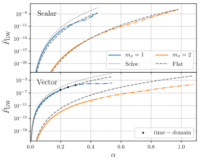
Figure 7: We show the mass-rescaled GW power $\tilde{P}_{\rm GW}$, defined in (30), emitted by the scalar and vector clouds with azimuthal number $m_{\sigma}=1$ and 2 at the saturation point, $\omega_{R}=m_{\sigma}\Omega_{H}$, comparing the Schwarzschild “Schw.” and the flat approximations to SuperRad (colored lines), and time-domain estimates obtained in East (2017, 2018). Dash-dotted colored lines indicate where SuperRad uses interpolation of numerical results over fits of the type (35).

In Figure 7, we compare the various calculation of the the GW power to the predictions by SuperRad. In the Newtonian limit, SuperRad differs from (31) due to the fit (35), allowing different leading-$\alpha$ coefficients. The underlying numerical results are more accurate (see Appendix E for details), allowing us to conclude that the estimates provided by SuperRad, are more accurate than the Schwarzschild or flat approximations. The analytic estimates for $\tilde{P}_{\rm GW}$ are worse for $m_{\sigma}=2$; we use those results only to inform the leading-$\alpha$ scaling behavior. We also show time-domain results from evolving the full nonlinear Einstein-Proca equations East (2017, 2018) for a few points. These agree with the Teukolsky calculations to within the numerical error of the simulations.

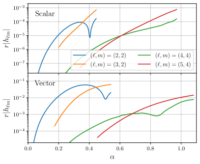
Figure 8: We show the magnitudes of the GW modes $h_{\ell m}$, defined in (26), which are sourced by $m_{\sigma}=1$ and $2$ scalar and vector boson clouds at saturation ($\omega_{R}=m_{\sigma}\Omega_{H}$) as functions of $\alpha$. Notice that $\ell\geq 2m_{\sigma}$.

In Figure 8, we show the GW modes provided by SuperRad, as defined in (26), over the entire parameter space, assuming the saturation condition. As expected from the non-relativistic results, the quadrupolar contribution $h_{22}$ dominates throughout most of the parameter space, except in the most relativistic regime, where $h_{32}$ increases in importance (and equivalently for $h_{44}$ and $h_{54}$). This behavior implies a constant phase shift between the two involved multipolar components. Hence, there is an $\alpha$-range where $|h_{22}|\sim|h_{32}|$ (and $|h_{44}|\sim|h_{54}|$), which means that the phase difference $\tilde{\phi}_{22}$ (and $\tilde{\phi}_{44}$), defined in (27), introduces a non-trivial phase-offset between the two involved polar modes.

VI Growth and decay of boson cloud

In this section, we address how the superradiant instability and GW calculations can be combined to calculate the evolution of the boson cloud, which determines the evolution of the amplitude and frequency of the GW signal.

A boson cloud around a spinning BH evolves as the cloud extracts energy and angular momentum from the BH through the superradiant instability. During this process, the cloud also loses energy and angular momentum to gravitational radiation. In a quasi-adiabatic approximation, the evolution of this system is given by

$$\begin{aligned} \dot{M_{c}}&=2\omega_{I}M_{c}+P_{\rm GW},\\ \dot{M}&=-2\omega_{I}M_{c},\\ \dot{J}&=-\frac{2m_{\sigma}\omega_{I}}{\omega_{R}}M_{c},\end{aligned}$$ (36)

where $\omega_{R}$, $\omega_{I}$, and $P_{\rm GW}$ are functions of the cloud mass and BH mass and spin. The evolution of the boson cloud can be roughly divided into two phases. In the first phase, the cloud grows exponentially, with the mass going like $M_{c}\sim\exp(2\omega_{I}t)$, with the growth eventually saturating as the BH is spun down and $\omega_{I}$ becomes small as $m_{\sigma}\Omega_{H}$ decreases towards $\omega_{R}$. This is followed by the gradual dissipation of the boson cloud through gravitational radiation. Since during this time $-\dot{M}_{c}\approx P_{\rm GW}\propto M_{c}^{2}$,

$$M_{c}(t)\approx\frac{\bar{M}_{c}}{1+(t-t_{\rm max})/\tau_{\rm GW}}$$ (37)

where the cloud mass reaches a maximum $\bar{M}_{c}$ at $t=t_{\rm max}$ and $\tau_{\rm GW}:=\bar{M}_{c}/P_{\rm GW}$.

In Figure 9, we plot an example of the evolution of the cloud mass for both scalar and vector bosons. In both cases, $\tau_{I}\ll\tau_{\rm GW}$, so that the exponential growth phase takes place on a much shorter time scale than GW dissipation. However, the ratio $\tau_{I}/\tau_{\rm GW}$ is markedly smaller in the scalar case compared to the vector one. In addition to the full evolution of the cloud as determined by (36), in Figure 9 we also plot a simple approximation where the maximum cloud mass is determined by solving for the BH parameters where $\omega_{R}=m_{\sigma}\Omega_{H}$, and the evolution of $M_{c}$ after the maximum is given solely by gravitational radiation, and the evolution of $M_{c}$ before the maximum is given by exponential growth with a fixed value $\omega_{I}$ given by the initial parameters.

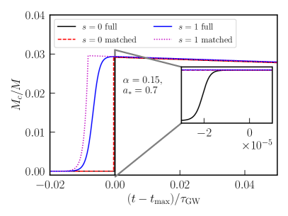
Figure 9: An example evolution of the boson cloud mass as a function of time for scalars ($s=0$) and vectors ($s=1$) with $\alpha=0.15$ and $a_{*}=0.7$. The plot compares the evolution determined by evolving the full equations (36) (solid lines, labelled “full”), to an approximation that matches together constant exponential growth to GW-dominated decay (dotted and dashed lines, labelled “matched”). Time is normalized by the gravitational dissipation timescale in either case, and the offset adjusted so that the maximum value of $M_{c}$ occurs at zero for the full evolution cases, and the matching value of $M_{c}$ is obtained for the corresponding matched evolution cases. The inset shows a zoom in of the end of the exponential growth phase for the scalar case (in particular the full evolution).

The SuperRad waveform model implements options for both the full cloud evolution and the matched approximation. While the latter approximation is less computationally expensive, as can be seen in Figure 9, it slightly overestimates the maximum cloud mass (by $\approx 0.04\%$ and $0.8\%$, respectively, for the scalar and vector cases shown in the figure), and underestimates the time for the cloud to reach its maximum. Thus, the more accurate full cloud evolution is appropriate for scenarios when the signal before the time when the cloud reaches saturation makes a non-negligible contribution. However, as noted above, our calculation of $\tilde{P}_{\rm GW}$ assumes $m_{\sigma}\Omega_{H}=\omega_{R}$, which is not strictly valid before the saturation of the instability. Hence, there will be a discrepancy in the BH spin used for the computation of the GW power. This discrepancy is negligible (i.e., below the numerical error of the methods, discussed in Appendix E) for $m_{\sigma}=2$, and for $m_{\sigma}=1$ assuming $a_{*}<0.9$. It should be noted that this affects the GW emission before saturation only, and also only systems with initial spin $a_{*}\gtrsim 0.9$. In the vector $m_{V}=1$ case, the largest discrepancy occurs for $\alpha\approx 0.46$ and extremal spins, where the relative error from assuming the saturation condition in the mass-rescaled GW power $\tilde{P}_{\rm GW}$ is $\approx 55\%$ (see Fig. 7 in Siemonsen and East (2020)). For the scalar $m_{S}=1$ case this discrepancy is at most $\approx 24\%$ around $\alpha\approx 0.36$.

VII LISA follow-up searches

The two main observational signatures of superradiant clouds, BH spin down and GW emission, are sensitive to various systematic and statistical uncertainties. Spin measurements have been used to exclude scalar and vector mass ranges. Most of these constraints, however, rely on BH-spin estimates from electromagnetic observations with significant systematic uncertainties. Spin measurements of BHs in inspiraling binaries using GWs exhibit large statistical uncertainties and make assumptions about the proceeding history of the binary. Constraints from the stochastic GW background, assuming a population of BH-cloud systems, rely on assumptions regarding the BH mass and spin population, in addition to position and distance uncertainties. Lastly, searches for GWs from existing BHs observed in the electromagnetic channel make assumptions about the past history of the observed BH, introducing large systematic uncertainties. Clearly all of these methods rely on modeling or assumptions with potentially substantial systematic uncertainties.

One search strategy for GWs from superradiant clouds, however, evades these assumptions: BH merger follow-up searches. These searches target BH remnants of previously detected compact binary coalescences. The key advantages are the knowledge of the complete past history of the targeted BH, as well as measurements of sky-position, spin, mass, and distance. Given these quantities, accurate predictions of the subsequent superradiance instability and GW emission are possible, enabling a targeted search for the latter in the days/weeks/years following the merger. This removes the assumptions affecting other search strategies, reduces the uncertainties to those coming from the merger GW signal measurement of the remnant, and those of the waveform model (discussed in the case of SuperRad below), and enables one to put confident constraints on relevant parts of the ultralight boson parameter space, or potentially to make a confident discovery.

In the context of the current generation of ground-based GW detectors, follow-up searches for GWs from scalar superradiant clouds are likely infeasible due to the small strain amplitudes Isi et al. (2019). On the other hand, because of their faster growth rates and orders of magnitude stronger signals, vector boson clouds are ideal candidates for these types of searches Jones et al. (prep). At design sensitivity, the advanced LIGO Aasi et al. (2015), advanced Virgo Acernese et al. (2015), and KAGRA Aso et al. (2013) observatories will in principle be sensitive to systems out to $\sim 1$ Gpc at a typical remnant BH spin of $a_{*}=0.7$ and masses of $M\sim 100M_{\odot}$ Chan and Hannuksela (2022); Jones et al. (prep). Undertaking follow-up searches targeting BHs falling into this parameter range could target vector boson masses roughly in the range of $\mathcal{M}_{V}\in(1\times 10^{-11},1\times 10^{-13})$ eV [see eq. (1)]. In a similar fashion, LISA could be sensitive to GWs from vector boson clouds with boson masses in the $\mathcal{M}_{V}<10^{-15}$ eV regime, inaccessible by ground-based detectors.

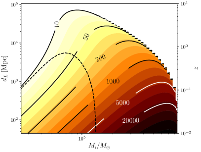
Figure 10: We show the SNR (contour lines and color) of GWs from vector superradiant clouds around a fiducial BH of initial remnant source frame mass of $M_{i}$ and spin $a_{*,i}=0.8$ as a function of luminosity distance $d_{L}$ and redshift $z$, assuming a standard $\Lambda$CDM cosmology and $\alpha=0.2$. For comparison, we also consider an initial spin of $a_{*,i}=0.7$ showing the $\rho_{\rm SNR}=10$ contour (dashed black line), assuming $\alpha=0.15$.

In the following, we analyze the prospects of follow-up searches for GWs from vector superradiant clouds around supermassive binary BH merger remnants with LISA. The fundamental assumption of follow-up searches is that a new superradiant cloud forms around the remnant after merger. If either of the constituents already posses a superradiant cloud, it is expected to be depleted before or during merger for nearly equal mass-ratio ($q\sim 1$) systems Baumann et al. (2019b). Even for $q>1$, depending on $\alpha$, clouds around the constituents of the binary are efficiently removed before merger Baumann et al. (2019b); Berti et al. (2019); Takahashi et al. (2022); Takahashi and Tanaka (2021). LISA is expected to see at least a handful of such mergers over the mission lifetime of four years Berti (2006); Micic et al. (2007). Therefore, to estimate the detection horizon, we assume a fiducial supermassive binary BH merger remnant detection that occurs one year into the mission. After merger at redshift $z$, residual ultralight vector densities around the remnant, or quantum fluctuations, trigger the superradiance instability leading to the complete cloud formation, and hence the peak of the GW signal, on timescales of at most $t_{c}\approx\tau_{I}(1+z)\log(M_{c}/\mathcal{M}_{V})/2$ in the detector frame. Over most of the parameter space, these signals will last for longer than the remaining three years of the LISA mission, leaving an observing time of $T_{\rm obs}=3-t_{c}$ years. We determine the maximum detection horizon of GWs from vector superradiant clouds by considering the optimal signal-to-noise ratio (SNR) $\rho_{\rm SNR}$ with the LISA sensitivity curve (details can be found in Appendix A). Making these assumptions, we illustrate the detection horizon of LISA for such events in Figure 10.

From Figure 10, we conclude that parts of the vector boson mass parameter space can be probed with idealized follow-up GW searches from supermassive binary BH remnants. Even for moderate initial spins of $a_{*,i}=0.7$, GWs can be detected up to $z\lesssim 0.8$, while for slightly more favorable initial spins of $a_{*,i}=0.8$, the GW emission is observable out to $z\lesssim 8$. The merger rate of massive BH binaries is expected to peak around $M\sim 10^{6}M_{\odot}$ for equal mass ratio systems, $q\lesssim 1$, and at $z\approx 2$ Mazzolari et al. (2022); Henriques et al. (2015); Izquierdo-Villalba et al. (2020). For initial BH masses $M_{i}>10^{6}\ M_{\odot}$, the cloud formation timescales are larger than the mission duration, $t_{c}>3$ years, leading to a drop in SNR. At high redshifts, the sensitivity of LISA is primarily limited by the short effective observation times in the detector frame. Larger BH masses (lower boson masses) can be accessed only with larger initial spins, or significantly longer mission durations. Consulting (1), vector boson masses roughly around $\mathcal{M}_{V}\in(1\times 10^{-16},6\times 10^{-16})$ eV are within reach of these follow-up search strategies with LISA.

These prospects are subject to a few caveats. First, we determined the detection horizon and sensitivity of LISA to GW from vector clouds around remnant supermassive BHs using the optimal matched filter SNR. What fraction of this total available SNR could be recovered from the data by a realistic search algorithm is an open question, even for ground-based detectors Jones et al. (prep). Secondly, the merger rate of massive BH binaries has large uncertainties. If the true merger rate were peaked at redshifts of $z>5$, a realistic follow-up search would require a very favorable initial BH spin $a_{*,i}>0.8$ to access a meaningful part of the vector boson parameter space directly, or an outlier event much closer.

VIII Discussion

We have introduced a new BH superradiance gravitational waveform model called SuperRad. This provides the superradiance instability growth timescale $\tau_{I}$, the cloud oscillation frequency $\omega_{R}$, the GW frequency $f_{\rm GW}(t)$ and strain $h_{\times/+}$ in the source frame as a function of time, the GW power $P_{\rm GW}$, and the evolution of the boson cloud. The SuperRad model makes use of all available analytic and numerical estimates for these observables, and calibrates analytic fits against the numerical data to extend the applicability across the entire parameter space of the $m=1$ and $2$ scalar and vector superradiant clouds. The waveform model SuperRad can be used to inform and interpret the results of GW searches for ultralight scalar and vector BH superradiance. This includes both blind and targeted searches for resolved continuous wave signals, as well as searches for a stochastic GW background from BH-boson cloud systems. It can also be used when interpreting BH spin measurements using GW or electromagnetic observations. Importantly, SuperRad is accurate in the relativistic regime where the observable signals will be the strongest.

As the ultralight boson cloud dissipates through gravitational radiation, there is a small increase in the frequency of the GWs due to the changing self-gravity contribution of the cloud. As illustrated above, even though this frequency drift is small, because of the large number of GW cycles that make up a typical superradiance signal, not properly accounting for it can lead to the signal model going out of phase in a fraction of the observing time. Fully including this second-order effect within BH perturbation theory is challenging, and the results in SuperRad for the frequency evolution of the GW signal use non-relativistic approximations. By comparing these to fully-relativistic numerical calculations for the scalar boson case, we found that the former underestimates the value of $\dot{f}_{\rm GW}$ by $\sim 30\%$ for the most relativistic (i.e. $\alpha\sim O(1)$) cases, though the differences are smaller for more typical parameters. In future work, we plan to include the fully-relativistic results for the cloud-mass contribution to the frequency for both scalar and vector bosons in SuperRad. Though, given the stringent accuracy requirements imposed by the typical signal timescales (see Fig. 5), it is likely that fully-coherent signal analysis techniques (e.g., match filtering) will still not be feasible in much of the parameter space, better predictions for the GW frequency evolution are nevertheless important in guiding the application of semi-coherent techniques.

Furthermore, we investigated the viability of follow-up searches for GWs from ultralight vector superradiant clouds with LISA targeting remnants of observed massive binary BH mergers. We found that these searches are confident probes of the ultralight vector boson parameter space around $\mathcal{M}\in(1\times 10^{-16},6\times 10^{-16})$ eV. With current estimates of the merger rate of massive BH binaries, LISA will be sensitive to GWs from vector boson clouds around remnants of these mergers out to redshift $z\lesssim 8$ at mass-ratio $q\lesssim 1$ and remnant black hole masses of roughly $M\in(6\times 10^{4},2\times 10^{5})M_{\odot}$. Our basic analysis leaves various questions unanswered. We assumed the total available signal-to-noise ratio can be recovered by a realistic search algorithm, which is an overestimate even in the case of ground-based detectors Jones et al. (prep). As well, a more detailed study folding in massive black hole binary merger rates with superradiant cloud growth timescales and emitted GW luminosities could provide an estimate for the expected number and mass ranges of merger events where LISA would be sensitive to the GW signal from an ultralight vector boson.

Appendix A LISA signal-to-noise ratio

For a given an initial BH spin and mass, as well as ultralight boson mass, SuperRad provides predictions for the GW strain $h_{+/\times}(t,R,\theta,\phi)$ at time $t$, (luminosity) distance $r$, and angles $(\theta,\varphi)$ in the source frame. In the case of LISA, the detector response functions $\tilde{X}_{+/\times}(\Theta,\Phi,\psi,f)$ relate the GW strain in the source frame to the strain in the detector. The latter depend on the source’s sky-position $(\Theta,\Phi)$, polarization $\psi$, and frequency $f$. Hence, the GW amplitude in the detector, $\tilde{h}_{\rm det.}(f)$, in the frequency domain is given by

$$\tilde{h}_{\rm det.}(f)=\tilde{X}_{+}\tilde{h}_{+}(f)+\tilde{X}_{\times}\tilde{h}_{\times}(f),$$ (38)

where $\tilde{h}_{+/\times}(f)$ are the Fourier-transforms of $h_{+/\times}(t,R,\theta,\varphi)$. Let $\langle\dots\rangle$ be the sky/polarization average over $\Theta$, $\Phi$, and $\psi$, and let $\mathcal{R}(f)$ be the frequency-dependent transfer function defined by the sky/polarization average of the detector response $\langle\tilde{h}_{\rm det.}^{*}\tilde{h}_{\rm det.}\rangle=\mathcal{R}(f)[|\tilde{h}_{\times}(f)|^{2}+|\tilde{h}_{+}(f)|^{2}]$. Then the SNR $\rho_{\rm SNR}$ is (see e.g., Refs. Robson et al. (2019); Babak et al. (2021))

$$\frac{\rho_{\rm SNR}^{2}}{4}=\int_{0}^{\infty}df\frac{\langle\tilde{h}_{\rm det.}^{*}\tilde{h}_{\rm det.}\rangle}{S_{n}(f)}=\int_{0}^{\infty}df\frac{|\tilde{h}_{\times}(f)|^{2}+|\tilde{h}_{+}(f)|^{2}}{S_{h}(f)},$$ (39)

where $S_{n}(f)$ is the noise power spectral density of LISA, and $S_{h}(f)=S_{n}(f)/\mathcal{R}(f)$ is the LISA sensitivity curve. For all estimates, we use the conservative six months confusion noise projections.

Since SuperRad provides the time domain GW strain in the source frame, we add the appropriate redshift factors and use fast-Fourier-transform algorithms to numerically transform into the frequency domain. This is feasible for shorter signals considered in follow-up searches. However, it becomes increasingly computationally expensive with longer signals at smaller $\alpha$.

Appendix B Superradiant field solutions

In this appendix, we briefly summarize the numerical methods we use to obtain the scalar and vector estimates for the oscillation frequencies $\omega_{R}$ and instability growth rates $\omega_{I}$ discussed in Secs. III.2 and III.3, respectively. We also provide bounds on the precision of our methods, and comment on the resulting uncertainties.

B.1 Scalar field

The real massive scalar wave equation (2) has been extensively studied in the context of asymptotically flat BHs. On a Kerr background of mass $M$ and spin parameter $a$, Detweiler Detweiler (1980) first derived expressions for the superradiance instability rates and oscillation frequencies. These results were refined in various other works, e.g., Refs. Dolan (2007); Yoshino and Kodama (2014); Baumann et al. (2019a). In this subsection, $\omega$, $\ell$, $n$, and $m$ refer exclusively to the scalar mode numbers, hence, we drop the subscripts used throughout the main text, for brevity.

Generally, due to the backgrounds symmetries, the most convenient scalar field ansatz is of the form $\Phi=\text{Re}[R_{s}(r)S_{s}(\theta)e^{-i(\omega t-m\varphi)}]$. With this ansatz, the field equations separate into a pair of polar and radial second-order ordinary differential equations. The polar equation can be identified with the spheroidal harmonic equation of spin-weight $s=0$ and spheriodicity $c^{2}=-k^{2}a^{2}$, with $k^{2}=\mu^{2}_{S}-\omega^{2}$; the solutions to this equation is the set of spheroidal harmonics, ${}_{s}\tilde{S}_{\ell m}(\theta;c)$, of spin-weight $s=0$. Hence, the polar solution is simply the spheroidal harmonic $S_{s}(\theta)={}_{0}\tilde{S}_{\ell m}(\theta;c)$ associated with the polar eigenvalue $A_{\ell m}(c)$ that reduces to $A_{\ell m}(c\rightarrow 0)=\ell(\ell+1)$ in the Schwarzschild limit (see, for instance, Ref. Berti et al. (2006)). The radial equation turns out to be the source-free $s=0$ radial Teukolsky equation

$$\begin{aligned} &\frac{d}{dr}\left(\Delta\frac{dR_{s}}{dr}\right)\\ &\quad+\left(\frac{(r^{2}+a^{2})\omega-am}{\Delta}-\lambda_{\ell m}-\mu^{2}_{S}r^{2}\right)R_{s}=0,\end{aligned}$$ (40)

where $\lambda_{\ell m}=A_{\ell m}+a^{2}\omega^{2}-2am\omega$ depends on the radial eigenvalue $\omega=\omega_{R}+i\omega_{I}$, and $\Delta=r^{2}-2Mr+a^{2}$.

The radial eigenvalue $\omega$ can be obtained, together with the radial solution $R_{s}(r)$ satisfying ingoing boundary conditions at the horizon, and asymptotically flat boundary conditions at spatial infinity. At leading order in $\alpha$, the above radial equation reduces to a type of Laguerre equation, yielding Hydrogen-like radial states, together with the associated energy spectrum $\omega$ Dolan (2007); Detweiler (1980). Higher order corrections at the level of the radial and polar equations are solved for in an order-by-order fashion perturbatively around $\alpha=0$. Solving the eigenvalue problem in this way leads to the higher order corrections to the real part of the superradiantly unstable scalar modes, defined in (9), Baumann et al. (2019a)

$$C_{S}[\alpha]=-\frac{\alpha^{4}}{8n^{4}}+\frac{f^{S}_{n\ell}\alpha^{4}}{n^{3}}+\frac{h^{S}_{\ell}a_{*}m\alpha^{5}}{n^{3}}+\mathcal{O}(\alpha^{6}),$$ (41)

where

$$\begin{aligned} f^{S}_{n\ell}=&\ -\frac{6}{2\ell+1}+\frac{2}{n},\\ h^{S}_{\ell}=&\ \frac{16}{2\ell(2\ell+1)(2\ell+2)}.\end{aligned}$$ (42)

The corresponding instability growth rates, defined in (13), are Detweiler (1980)

$$\begin{aligned} G_{S}(a_{*},\alpha)=&\ \frac{2^{4\ell+1}(n+\ell)!}{n^{2\ell+4}(n-\ell-1)!}k^{S}_{n\ell}g^{S}_{m\ell}\\ k^{S}_{n\ell}=&\ \left[\frac{\ell!}{(2\ell)!(2\ell+1)!}\right]^{2},\\ g^{S}_{m\ell}=&\ \prod_{o=1}^{\ell}\left[o^{2}(1-a_{*}^{2})+(a_{*}m-2r_{+}\omega_{R})^{2}\right].\end{aligned}$$ (43)

for the most unstable mode in the non-relativistic limit. The principle quantum number $n$ is defined in (10).

In this work, we compute the eigenvalue $\omega=\omega_{R}+i\omega_{I}$ numerically in the relativistic regime $\mathcal{D}_{\rm int}$ where the analytic methods break down. The typical approach employed to solve differential eigenvalue problems of this type goes back to Leaver Leaver (1985), and was applied to massive scalar fields in Kerr spacetime in Refs. Dolan (2007); Yoshino and Kodama (2014). There, the radial solution is assumed to be written in power series form as

$$R(r)=(r-r_{+})^{-i\beta}(r-r_{-})^{i\beta+\gamma-1}\sum_{n\geq 0}a_{n}\left(\frac{r-r_{+}}{r-r_{-}}\right)^{n},$$ (44)

with $\beta=2Mr_{+}(\omega-m\Omega_{H})/(r_{+}-r_{-})$ and $\gamma=M(2\omega^{2}-\mu^{2}_{S})/k$. Plugging this into the radial equation (40), one obtains a recurrence relation between the coefficients $a_{n}$. This relation is used to obtain a continued fraction constraint on the frequency $\omega$ for each $\{\ell,m,a,\mu_{S}\}$. This constraint is an implicit equation for the eigenvalues $\omega_{R}$ and $\omega_{I}$, which can be solved for numerically using a minimization algorithm over the complex $\omega$-plane. With the recurrence relation and $\omega$, the radial solution is constructed using (44). Details can be found in Refs. Dolan (2007); Yoshino and Kodama (2014). In the non-relativistic limit, we found that a total number of $N\geq 5000$ terms in the series expansion is necessary for our desired accuracy, while in the relativistic regime, a lower number, i.e., $N\leq 1000$, is sufficient. We construct the spheroidal harmonics ${}_{0}S_{\ell m}(\theta;c)$ and associated eigenvalues $A_{\ell m}$ using qnm, a python implementation of a Leaver-like continued fraction method developed in Ref. Stein (2019).

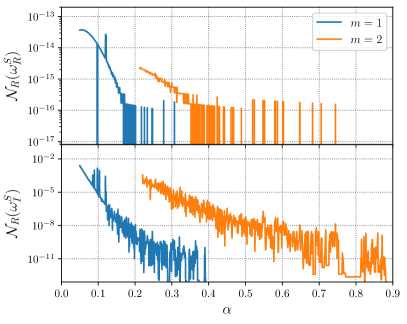
Figure 11: The relative numerical error $\mathcal{N}_{R}$, defined in (45), of the real and imaginary parts of the frequency of the scalar $m=1$ and $m=2$ superradiant states around a BH of spin $a_{*}=0.985$.

In order to estimate the numerical uncertainty of this method, we determine the frequency $\omega$ in a range of $\alpha$ and fixed BH spin, using the above approach with successively increasing $N$, up to the $N_{\rm max}=8000$ used throughout the entire parameter space in SuperRad. The numerical error is then estimated by

$$\mathcal{N}_{R}(\omega)=\frac{|\omega_{N_{\rm max}}-\omega_{N_{\rm max}/2}|}{\omega_{N_{\rm max}}}.$$ (45)

The results are shown in Figure 11. We ensure that the minimization algorithm has termination conditions at the floating point level. The real part of the frequency is obtained to one part in $\sim 10^{14}$, whereas the imaginary part is determined less precisely. However, even for $\alpha\gtrsim 0.05$, the latter is more precise or comparable to the theoretical uncertainty of the analytic estimates in (9) together with (41). This establishes the numerical uncertainties of the methods used to extend SuperRad into the relativistic regime. However, it does not show the overall uncertainty of SuperRad in this regime due to interpolation error, which is discussed in Appendix C.

B.2 Vector field

The massive vector wave equation (2) has been studied more recently in Pani et al. (2012b); Cardoso et al. (2018); Dolan (2018); Frolov et al. (2018). The non-separability of the vector field equation was a fundamental problem until a series of works by Lunin Lunin (2017) and Frolov et al. Frolov et al. (2018). There, an ansatz, referred to as FKKS in the following, was constructed that separates the polar and radial parts of the field equation (2), and hence, significantly simplifies the problem. We briefly summarize this ansatz and quote analytic results for the oscillation frequency and instability growth rates, $\omega=\omega_{R}+i\omega_{I}$, obtained with it. Similarly to the previous subsection, we drop the subscripts of $\omega,\ell,n$, and $m$, used in the main text, and use these exclusively for vector modes and frequencies.

The FKKS ansatz exploits a hidden symmetries of Kerr spacetime $g_{\mu\nu}$. This symmetry is captured by a Killing-Yano 2-form k, with tensor components that satisfy $\nabla_{\alpha}k_{\beta\gamma}=2g_{\alpha[\beta}\xi_{\gamma]}$. Using this, the vector field ansatz takes the form

$$A^{\mu}=B^{\mu\nu}\nabla_{\nu}Z, Z=R_{V}(r)S_{V}(\theta)e^{-i(\omega t-m\varphi)},$$ (46)

with polarization tensor $B^{\mu\nu}(g_{\nu\gamma}+i\nu k_{\nu\gamma})=\delta^{\mu}_{\gamma}$ and angular eigenvalue $\nu$. Plugging this ansatz into (2) yields ordinary differential equations for the radial and polar dependencies, respectively. The angular equation is a deformed spheroidal harmonic equation for spin-weight $s=-1$ that does not, a priori, possess known solutions. In the Schwarzschild limit, $a\rightarrow 0$, the solutions reduce the usual spherical harmonics $S_{V}(\theta)=Y_{\ell m}(\theta)$, with a relation between the polar eigenvalue $\Lambda=\ell(\ell+1)$ and the separation constant $\nu\rightarrow\nu_{\ell}$ (see Ref. Dolan (2018) for details). In this limit, the spatial components of the vector field are then given by $A^{i}_{a\rightarrow 0}\propto Y^{i}_{j,jm}(\theta)$ where $Y^{i}_{j,jm}(\theta)$ are the vector spherical harmonics with $j=\ell-\hat{S}$ (see Ref. Thorne (1980)). When the BH spin is non-zero, there is a mixing of the polar mode number $\ell$, such that, in general $S_{V}(\theta)=Y_{|m|,m}(\theta)+b_{1}Y_{|m|+1,m}(\theta)+\dots$. The radial equation for $R_{V}(r)$ takes the form

$$\mathcal{D}_{\nu,\omega,m,a}R_{V}(r)=0,$$ (47)

with a second order differential operator $\mathcal{D}_{\nu,\omega,m,a}$ Frolov et al. (2018); Dolan (2018). In the $a\rightarrow 0$ limit, and at leading order in $\alpha$, this equation reduces to a Schrödinger-type equation for $R_{V}(r)$ with the eigenvalue spectrum (9) Baryakhtar et al. (2017). This FKKS ansatz was used in Baumann et al. (2019a) to go beyond the leading orders in both $a$ and $\alpha$. They found the sub-leading corrections to the spectra (9) to be

$$C_{V}[\alpha]=-\frac{\alpha^{4}}{8n^{4}}+\frac{f^{V}_{n\ell\hat{S}}\alpha^{4}}{n^{3}}+\frac{h^{V}_{\ell\hat{S}}a_{*}m\alpha^{5}}{n^{3}}+\mathcal{O}(\alpha^{6}),$$ (48)

with

$$f^{V}_{n\ell\hat{S}}= \ -\frac{4(6\ell(\ell-\hat{S}+1)-3\hat{S}+2)}{(2\ell-\hat{S})(2\ell-\hat{S}+1)(2\ell-\hat{S}+2)}+\frac{2}{n},$$ (49)

$$h^{V}_{\ell\hat{S}}= \ \frac{16}{(2\ell-\hat{S})(2\ell-\hat{S}+1)(2\ell-\hat{S}+2)}.$$ (50)

The corresponding instability growth rates (13) are Baryakhtar et al. (2021); Baumann et al. (2019a)

$$\begin{aligned} G_{V}(a_{*},\alpha)=&\ \frac{2^{4\ell-2\hat{S}+1}(n+\ell)!}{n^{2\ell+4}(n-\ell-1)!}k^{V}_{\ell\hat{S}}d^{V}_{\ell\hat{S}}g^{V}_{\ell\hat{S}}\\ k^{V}_{\ell\hat{S}}=&\ \left[\frac{\ell!}{(2\ell-\hat{S})!(2\ell-\hat{S}+1)!}\right]^{2},\\ d^{V}_{\ell\hat{S}}=&\ \left[1+\frac{2(1+\hat{S})(1-\hat{S})}{2\ell-\hat{S}}\right]^{2},\\ g^{V}_{\ell\hat{S}}=&\ \prod_{o=1}^{\ell-\hat{S}}\left[o^{2}(1-a_{*}^{2})+(a_{*}m-2r_{+}\omega_{R})^{2}\right].\end{aligned}$$ (51)

for the most unstable mode in the non-relativistic limit, $\ell=m+\hat{S}$ and $\hat{S}=-1$.

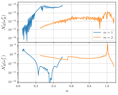
Figure 12: The relative numerical error $\mathcal{N}_{R}$ of the real and imaginary parts of the frequency of the vector $m=1$ and $m=2$ superradiant states around a BH of spin $a_{*}=0.985$.

In this work, we obtain numerical data in the relativistic regime $\mathcal{D}_{\rm int}$ by solving (47) and the associated polar equation numerically following Refs. Dolan (2018); Siemonsen and East (2020). To that end, the angular equation is expanded in regular spherical harmonics ${}_{0}S_{\ell m}(\theta;c=0)$, while the radial equation is integrated numerically outwards from the horizon to large distances. Therefore, as long as a sufficient number of terms is considered in the polar sector, the numerical uncertainties are dominated by the integration method used in the radial sector. We make use of the BHPToolkit to construct spherical and spheroidal harmonics BHP . In order to obtain estimates for the numerical uncertainty, we vary the step size of the radial numerical integration. In Figure 12, we show upper bounds on the relative numerical uncertainty of the method described above to obtain the frequencies $\omega$. As in the scalar case, the numerical uncertainty of the underlying numerical methods is below the interpolation error of SuperRad discussed in the next section.

Appendix C Interpolation and Extrapolation Error of SuperRad

The uncertainties associated to the values of $\tau_{I}=1/\omega_{I}$ and $f_{\rm GW}=\omega_{R}/\pi$ provided by SuperRad come from an interplay of interpolation errors, numerical errors, truncation errors of analytic expressions, and the theoretical assumptions made. Furthermore, due to the combination of methods involved, the overall uncertainty of SuperRad varies across the parameter space. In this appendix, we provide justifications for accuracy claims made in the main text, as well as establish upper bounds for uncertainties of the observables contained in SuperRad.

As we show below, we find the interpolation and extrapolation error to be the dominant source of error for the waveform model, subdominant to the truncation error described in the previous section, and shown in Figure 11 and Figure 12. As described in the main text, and shown in Figure 2, in the relativistic regime labelled $\mathcal{D}_{\rm int}$, SuperRad uses linear interpolation functions to interpolate based on a grid of $320^{2}$ data points. We quantify the interpolation error by directly computing the value of $\omega_{R}$ and $\omega_{I}$ at intermediate value to these data points using the methods outlined in the previous section, and compare them to the interpolated value. Similarly, we can directly compute the values of $\omega_{R}$ and $\omega_{I}$ in the non-relativistic regime $\mathcal{D}_{\rm fit}$, again using the accurate numerical methods from the previous section, and compare them to their extrapolated values obtained using the fits.

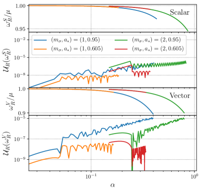
Figure 13: We show a set of representative frequencies $\omega_{R}$ of a $m_{\sigma}=1$ and $2$ scalar (top) and vector (bottom) mode (with $\ell_{S}=m_{S}$ and $\hat{S}=-1$, respectively), assuming a BH spin of $a_{*}\in\{0.605,0.95\}$, obtained by SuperRad. We also plot the relative interpolation/extrapolation error $\mathcal{U}_{R}$ of these predictions (see the main text for discussion).

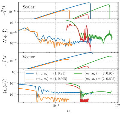
Figure 14: We show a set of representative growth rates $\omega_{I}^{\sigma}$ of a $m_{\sigma}=1,2$ scalar (top) and vector (bottom) mode (with $\ell_{S}=m_{S}$ and $\hat{S}=-1$, respectively), assuming a BH spin of $a_{*}\in\{0.6,0.95\}$, obtained by SuperRad. We also plot the relative interpolation/extrapolation error $\mathcal{U}_{R}$ of these predictions (see the main text for discussion).

In Figure 13 and Figure 14, we show the relative error in interpolating or extrapolating $\omega_{R}$ and $\omega_{I}$ to a given point in SuperRad, compared to directly computing the value at that point $\mathcal{U}_{R}(x)=|x-x_{\rm num.}|/x_{\rm num.}$. We show this for two fiducial spin values $a_{*}\in\{0.605,0.95\}$ across the $\alpha$-parameter space from a region in $\mathcal{D}_{\rm fit}$ to the entire $\mathcal{D}_{\rm int}$ at that spin. The uncertainty is relatively low in the relativistic regime $\mathcal{D}_{\rm int}$, spanning from $\alpha^{m_{\sigma}=1}=0.05$ and $\alpha^{m_{\sigma}=2}=0.25$ to maximal $\alpha$. There, the relative uncertainty in the frequency $\omega_{R}$ does not exceed $\sim 10^{-5}$, while in the case of the growth rates $\omega_{I}$, it is bounded by $\sim 10^{-2}$. In the extrapolated region $\mathcal{D}_{\rm fit}$, spanning from $\alpha^{m_{\sigma}=1}=0.05$ and $\alpha^{m_{\sigma}=2}=0.25$ towards small $\alpha$, the uncertainty $\mathcal{U}_{R}(\omega_{R})$ of the frequencies is well under control and decreases in the Newtonian limit. The growth rates, on the other hand, show larger uncertainties transitioning from $\mathcal{D}_{\rm int}$ towards smaller $\alpha$. The fitting procedure, in this case, is more complex, which is reflected in the choices of $p$ and $q$ required for (15) (noted below) to be below or comparable to the difference between the purely analytic expressions and the numerical expressions obtained in parts of $\mathcal{D}_{\rm fit}$. The fit functions and the purely analytic estimates for $\omega_{I}$ have comparable accuracy for $\alpha\lesssim 0.05$ and $\alpha\lesssim 0.25$ for $m_{\sigma}=1$ and $m_{\sigma}=2$, respectively. The uncertainties are, by construction, decreasing at sufficiently small $\alpha$, while there remains an intermediate regime around $\alpha\approx 0.02$ for $m_{\sigma}=1$ and $\alpha\approx 0.2$ for $m_{\sigma}=2$, where the uncertainties first increase. This is a result of the lack of accurate analytical or numerical modeling in this regime. Lastly, since all numerical errors discussed in the previous appendices are below the uncertainties presented here, the latter can be understood as the overall uncertainties of the waveform model. Furthermore, comparing the uncertainties $\mathcal{U}_{R}$ presented here to the relative differences in Figure 3 and Figure 4, we see that the latter is always smaller or comparable to the former. We comment on the uncertainties in the GW emission in Appendix E. As can be seen in the temporal evolution of the GW frequency emitted by an $m_{S}=1$ scalar cloud in Figure 1, the quantities (frequencies, timescales, frequency drifts etc.) exhibit a small discontinuity at the interface of $\mathcal{D}_{\rm fit}$ and $\mathcal{D}_{\rm int}$. This is important only, when the system is evolved adiabatically using (36), not when the saturation condition $\omega_{R}=m_{\sigma}\Omega_{H}$ is used to set the GW amplitude.

For completeness, we list the different domains $\mathcal{D}_{\rm int}$ used in SuperRad here. These domains are all bounded by the superradiance saturation condition $\omega_{R}=m_{\sigma}\Omega_{H}(a_{*})$ at sufficiently large $\alpha$, and by $a_{*}=0.6$ and $a_{*}=0.995$. At small $\alpha$ the regions $\mathcal{D}_{\rm int}$ are bounded by $\alpha_{m_{\sigma}=1}=0.05$ and $\alpha_{m_{\sigma}=2}=0.25$ for both the scalar and the vector clouds. The fit functions for $\omega_{R}$ in (11) contain the following terms: For $m_{V}=1$ and $2$ and $m_{S}=1$ and $2$, we set $q\in\{0,1,\dots,3\}$ and $p\in\{6,7,8\}$. In all four cases, we added the term $\alpha^{5}a_{*}(\sqrt{1-a_{*}^{2}}-1)$. The fit functions for $\omega_{I}$ in (15) contain the following terms: For $m_{V}=1$, we set $p\in\{1,2,\dots,10\}$, and $q\in\{0,1\}$; for $m_{V}=2$ we set $p\in\{5,6,\dots,10\}$ and $q\in\{0,1\}$; for $m_{S}=1$ we set $p\in\{1,2,3\}$ and $q\in\{0,1,\dots,3\}$; for $m_{S}=2$ we alter the fit function slightly with $\hat{c}_{p,q}\rightarrow\delta_{q,1}\hat{c}_{p}$ and $\hat{b}_{p,q}\rightarrow\alpha^{2}\hat{b}_{p,q}/a_{*}$ with $p\in\{12,\dots,22\}$ and $q\in\{0,1,\dots,3\}$. These were fit against the numerical data in $\mathcal{D}_{\rm int}$ with $\alpha<\alpha_{\rm bound}$, where $\alpha_{\rm bound}^{m_{\sigma}=1}=0.25$ and $\alpha_{\rm bound}^{m_{\sigma}=2}=0.6$.

Appendix D Frequency shift

In this appendix, we briefly discuss the leading-in-$\alpha$ contribution to the shift in frequency due to the self-gravity of the cloud $\Delta\omega_{\sigma}=\alpha^{3}M_{c}F_{\sigma}/M^{2}$, where $F_{\sigma}$ is defined in (22), as described in Sec. IV. For the scalar and vector boson clouds, these are given by

$$\begin{aligned} F_{S}&=\bar{F}[m_{S}],\\ F_{V}&=\bar{F}[m_{V}-1],\end{aligned}$$ (52)

where

$$\bar{F}[b]=-\frac{2(b+1)\sqrt{\pi}\Gamma(2(b+1))-\Gamma\left(2b+\frac{5}{2}\right)}{2(b+1)^{3}\sqrt{\pi}\Gamma(2(b+1))}.$$ (53)

$m_{V}$	$m_{S}$	$M^{2}\Delta\omega_{\sigma}/(M_{c}\alpha^{3})$
1	-	$-5/8$
2	1	$-93/512$
3	2	$-793/9216$
4	3	$-26333/524288$
5	4	$-43191/1310720$
6	5	$-1172755/50331648$

Table 1: We list the first few leading-in-$\alpha$ contributions to the frequency shift $\Delta\omega_{\sigma}=\alpha^{3}M_{c}F_{\sigma}/M^{2}$ for the oscillation frequency of scalar and vector clouds.

In Table 1, we present explicit values for $m_{\sigma}=1,\dots,5$ for both the scalar and vector cases. The frequency shift monotonically decreases with increasing $m_{\sigma}$. The shift depends (to leading order in $\alpha$) only on the $\ell_{\sigma}$ mode number of the considered field, i.e., the Bohr radius of these non-relativistic solutions, which determines $F_{\sigma}$, is dependent on the $\ell_{\sigma}$ mode number only.

Appendix E Gravitational waves

In this appendix, we outline the frequency-domain methods used in the literature and this work to determine the GWs emitted from a superradiant cloud after the saturation of the instability, i.e., assuming $\omega_{R}=m_{\sigma}\Omega_{H}(a_{*})$. In the context of the Teukolsky formalism for linear perturbations on a fixed Kerr spacetime $g_{\mu\nu}$, finding the GW power and strain reduces to finding the Weyl-Newman-Penrose scalar $\Psi_{4}$ at large distances. To that end, the field equations for linear metric perturbations on $g_{\mu\nu}$ are solved using a separation ansatz similar to the one used in the previous sections. The polar equation is the defining equation for spin-weighted spheroidal harmonics, while schematically the sourced radial Teukolsky equation takes the form Teukolsky (1973)

$$\mathcal{D}^{a,M}_{\ell m\omega}R_{\ell m\omega}(r)=\hat{T}_{\ell m\omega}(r),$$ (54)

with sources $\hat{T}_{\ell m\omega}$. In this appendix, $\ell,m$, and $\omega$ refer exclusively to modes characterizing the metric perturbations, not the states of the superradiant clouds. The second order radial differential operator $\mathcal{D}^{a,M}_{\ell m\omega}$, for a Kerr spacetime of mass $M$ and spin parameter $a$, is of Sturm-Liouville type and, hence, allows for the generic construction of a Green’s function to solve the inhomogeneous problem ($\hat{T}_{\ell m\omega}\neq 0$) given the set of homogeneous solutions $R^{H}_{\ell m\omega}$ satisfying purely ingoing and purely outgoing boundary conditions at the horizon, $r=r_{+}$, and infinity, $r\rightarrow\infty$, respectively. At large distances $r$, the solution to the radial Teukolsky equation is

$$\begin{aligned} R_{\ell m\omega}(r\rightarrow\infty)=&\ \frac{r^{3}e^{i\omega r_{*}}}{2i\omega B_{\ell m\omega}}\int_{r_{+}}^{\infty}dr^{\prime}\frac{\hat{T}_{\ell m\omega}R^{H}_{\ell m\omega}}{\Delta^{2}}\\ =&\ Z^{\infty}_{\ell m}r^{3}e^{i\omega r_{*}}.\end{aligned}$$ (55)

Here, $r_{*}$ is the Tortoise coordinate of $r$, and we defined a set of variables $Z^{\infty}_{\ell m}$ containing information about the source (see, e.g., Ref. Siemonsen and East (2020), for details). With this in hand, the GWs at infinity can be calculated as

$$\Psi_{4}=\frac{1}{r}\sum_{\ell,m}\frac{Z^{\infty}_{\ell m}}{\sqrt{2\pi}}e^{i\omega(r_{*}-t)}{}_{-2}S_{\ell m}(\theta;c=a\omega)e^{im\varphi}.$$ (56)

Notice, the summation in (56) is over spheroidal $\ell$, rather than spherical $\ell$ as done in Sec. V.1. Here, we are using the normalization $\int d\cos\theta|{}_{-2}S_{\ell m}(\theta;c)|^{2}=1$. To recover the spherical harmonic GW modes $h^{\ell^{\prime}m^{\prime}}$, we rewrite the above, using

$$h=-\frac{2\Psi_{4}}{(2\omega_{R})^{2}},$$ (57)

leading to

$$re^{i\omega t}h^{\ell^{\prime}m^{\prime}}=\sum_{\ell,m}\frac{-2Z^{\infty}_{\ell m}}{\sqrt{2\pi}(2\omega_{R})^{2}}C^{\ell^{\prime}m^{\prime}}_{\ell m}=\frac{-2\tilde{Z}^{\infty}_{\ell^{\prime}m^{\prime}}}{\sqrt{2\pi}(2\omega_{R})^{2}},$$ (58)

with

$$C^{\ell^{\prime}m^{\prime}}_{\ell m}=\int_{S^{2}}d\Omega{}_{-2}\bar{Y}_{\ell^{\prime}m^{\prime}}(\Omega){}_{-2}S_{\ell m}(\theta;c=a\omega)e^{im\varphi}.$$ (59)

Note that when $c=0$, $C^{\ell^{\prime}m^{\prime}}_{\ell m}=2\pi\delta^{\ell^{\prime}}_{\ell}\delta^{m^{\prime}}_{m}$. The total emitted gravitational energy flux is

$$P_{\rm GW}=\sum_{\ell^{\prime},m^{\prime}}\frac{|\tilde{Z}^{\infty}_{\ell^{\prime}m^{\prime}}|^{2}}{8\pi^{2}(2\omega_{R})^{2}}.$$ (60)

Therefore, determining the GWs emitted depends on finding homogeneous solutions to the radial Teukolsky equation, as well as integrating these over the cloud sources $\hat{T}_{\ell m\omega}$. The three distinct approximations mentioned in the main text—flat, Schwarzschild, and Teukolsky—all emerge from (55) by dropping certain terms. In the flat approximation, the spin is neglected, $a=0$, and the source equations are expanded to leading order in $\alpha$, implying $M\rightarrow 0$. In this limit, both the homogeneous solutions and source functions can be constructed and integrated over analytically. In the Schwarzschild approximation, one also expands in $\alpha$ to leading order and assumes $a=0$. However, one includes the gravitational potential terms present in the Schwarzschild Green’s function, i.e., $M\neq 0$. For $\ell^{\prime}=m^{\prime}=2$, the flat ansatz generally underestimates the emitted GW flux, while the Schwarzschild approximation overestimates the power. Solving the equation (54) numerically making no assumptions about $\alpha$ or $a$ (referred to as the Teukolsky approximation in the main text) provides the most accurate predictions for $P_{\rm GW}$ and $h$, and is expected to give values intermediate to the flat and the Schwarzschild approximations. More details can be found in, for instance, Refs. Brito et al. (2017a); Baryakhtar et al. (2017).

For $\ell^{\prime}=m^{\prime}>2$, i.e., $m_{\sigma}>1$, the GW energy flux has been computed analytically only in the flat approximation. In the scalar case, the total GW power emitted from a cloud with $(n_{S},m_{S})$ and $\ell_{S}=m_{S}$, is given by Yoshino and Kodama (2014)

$$P_{\rm GW}=C_{n_{S}m_{S}}\alpha^{Q_{S}}\frac{M_{c}^{2}}{M^{2}},$$ (61)

where $Q_{S}=4m_{S}+10$ and

$$\begin{aligned} C_{n_{S}m_{S}}=\frac{16^{m_{S}+1}m_{S}(2m_{S}-1)}{n_{S}^{4m_{S}+8}(m_{S}+1)\Gamma(m_{S}+1)^{4}}\\ \times\frac{\Gamma(2m_{S}-1)^{2}\Gamma(m_{S}+n_{S}+1)^{2}}{\Gamma(4m_{S}+3)\Gamma(n_{S}-m_{S})^{2}}.\end{aligned}$$ (62)

In the vector case, for $m^{\prime}>1$, the GW power emitted from a $\hat{S}=-1$ superradiant state in the $\alpha\ll 1$ limit is Baryakhtar et al. (2017)

$$P_{\rm GW}=K_{m_{V}}\alpha^{Q_{V}}\frac{M_{c}^{2}}{M^{2}},$$ (63)

where $Q_{V}=4m_{V}+6$, $K_{2}=1/126,K_{3}=6\times 10^{-6},K_{4}=2\times 10^{-9}$, and $K_{5}=4\times 10^{-13}$.

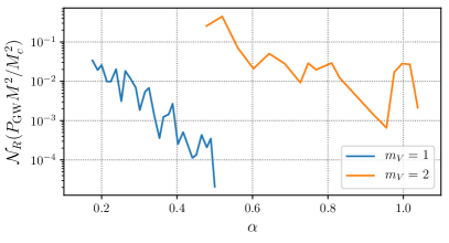
Figure 15: The relative numerical error $\mathcal{N}_{R}$ of the total emitted GW energy flux $P_{\rm GW}$ from a vector cloud in the $m_{V}=1$ and $m_{V}=2$ superradiant states around a BH of spin $a=0.985M$ in the relevant part of the parameter space.

The specifics of the methods we use to numerically solve (54) are discussed in detail in Ref. Siemonsen and East (2020) (we make use of the BHPToolkit BHP ). It involves constructing the sources $\hat{T}_{\ell m\omega}$ from the numerical superradiant solutions to (2), and integrating (55) numerically. In Figure 15, we present upper bounds on the numerical error of these methods across the entire parameter space, assuming a $m_{V}=1$ and $2$ vector cloud (analogous upper bounds are expected for scalar clouds). The bounds are obtained from varying the resolution of the underlying superradiant vector field solution together with the radial step size of the numerical integration of (55). The relative difference between estimates of $\tilde{P}_{\rm GW}$ with two different resolutions decreases with increasing resolution. The upper bounds shown in Figure 15 are the relative difference between the default resolution used throughout, and half that resolution. As for the GW power calculation, the GW strain $h$ is calculated from the solutions to (55), through (58). Since $h\sim\sqrt{P_{\rm GW}}$, the values for $\mathcal{N}_{R}(\tilde{P}_{\rm GW})$ can be interpreted as an estimate for the error $\mathcal{N}_{R}(h_{\times,+}M/M_{c})$ for the amplitudes of the polarization waveform.

Lastly, the numerical data regimes $\tilde{D}_{\rm int}$ (defined in Sec. V.2) is bounded at large $\alpha$ by the maximal $\alpha$ satisfying the superradiance saturation condition $\omega_{R}=m_{\sigma}\Omega_{H}$ at the corresponding spin $a_{*}$. From below, it is bounded by $\alpha_{\rm low}^{m_{S}=1}=0.2$ and $\alpha_{\rm low}^{m_{S}=2}=0.34$, for scalars and the two lowest azimuthal numbers, and $\alpha_{\rm low}^{m_{V}=1}=0.17$ and $\alpha_{\rm low}^{m_{V}=2}=0.45$, for vectors with the two lowest azimuthal numbers.

References

- Starobinsky (1973) A. A. Starobinsky, Sov. Phys. JETP 37, 28 (1973).
- Zel’Dovich (1971) Y. B. Zel’Dovich, Soviet Journal of Experimental and Theoretical Physics Letters 14, 180 (1971).
- Penrose and Floyd (1971) R. Penrose and R. M. Floyd, Nature 229, 177 (1971).
- Arvanitaki et al. (2010) A. Arvanitaki, S. Dimopoulos, S. Dubovsky, N. Kaloper, and J. March-Russell, Phys. Rev. D 81, 123530 (2010), arXiv:0905.4720 [hep-th] .
- Peccei and Quinn (1977) R. D. Peccei and H. R. Quinn, Phys. Rev. Lett. 38, 1440 (1977).
- Weinberg (1978) S. Weinberg, Phys. Rev. Lett. 40, 223 (1978).
- Wilczek (1978) F. Wilczek, Phys. Rev. Lett. 40, 279 (1978).
- Essig et al. (2013) R. Essig et al., in Proceedings, 2013 Community Summer Study on the Future of U.S. Particle Physics: Snowmass on the Mississippi (CSS2013): Minneapolis, MN, USA, July 29-August 6, 2013 (2013) arXiv:1311.0029 [hep-ph] .
- Hui et al. (2017) L. Hui, J. P. Ostriker, S. Tremaine, and E. Witten, Phys. Rev. D95, 043541 (2017), arXiv:1610.08297 [astro-ph.CO] .
- Marsh (2016) D. J. E. Marsh, Phys. Rept. 643, 1 (2016), arXiv:1510.07633 [astro-ph.CO] .
- Goodsell et al. (2009) M. Goodsell, J. Jaeckel, J. Redondo, and A. Ringwald, JHEP 11, 027 (2009), arXiv:0909.0515 [hep-ph] .
- Jaeckel and Ringwald (2010) J. Jaeckel and A. Ringwald, Ann. Rev. Nucl. Part. Sci. 60, 405 (2010), arXiv:1002.0329 [hep-ph] .
- Clifton et al. (2012) T. Clifton, P. G. Ferreira, A. Padilla, and C. Skordis, Phys. Rept. 513, 1 (2012), arXiv:1106.2476 [astro-ph.CO] .
- Ternov et al. (1978) I. M. Ternov, V. R. Khalilov, G. A. Chizhov, and A. B. Gaina, Sov. Phys. J. 21, 1200 (1978).
- Zouros and Eardley (1979) T. J. M. Zouros and D. M. Eardley, Annals Phys. 118, 139 (1979).
- Detweiler (1980) S. L. Detweiler, Phys.Rev. D22, 2323 (1980).
- Dolan (2007) S. R. Dolan, Phys. Rev. D 76, 084001 (2007), arXiv:0705.2880 [gr-qc] .
- Arvanitaki and Dubovsky (2011) A. Arvanitaki and S. Dubovsky, Phys. Rev. D 83 (2011), 10.1103/PhysRevD.83.044026.
- Yoshino and Kodama (2014) H. Yoshino and H. Kodama, PTEP 2014, 043E02 (2014), arXiv:1312.2326 [gr-qc] .
- Arvanitaki et al. (2015) A. Arvanitaki, M. Baryakhtar, and X. Huang, Phys. Rev. D 91 (2015), 10.1103/PhysRevD.91.084011.
- Arvanitaki et al. (2017) A. Arvanitaki, M. Baryakhtar, S. Dimopoulos, S. Dubovsky, and R. Lasenby, Phys. Rev. D 95 (2017), 10.1103/PhysRevD.95.043001.
- Brito et al. (2015a) R. Brito, V. Cardoso, and P. Pani, Class. Quant. Grav. 32, 134001 (2015a), arXiv:1411.0686 [gr-qc] .
- Yoshino and Kodama (2015) H. Yoshino and H. Kodama, Class. Quant. Grav. 32, 214001 (2015), arXiv:1505.00714 [gr-qc] .
- Rosa and Dolan (2012) J. G. Rosa and S. R. Dolan, Phys. Rev. D85, 044043 (2012), arXiv:1110.4494 [hep-th] .
- Pani et al. (2012a) P. Pani, V. Cardoso, L. Gualtieri, E. Berti, and A. Ishibashi, Phys. Rev. Lett. 109, 131102 (2012a), arXiv:1209.0465 [gr-qc] .
- Pani et al. (2012b) P. Pani, V. Cardoso, L. Gualtieri, E. Berti, and A. Ishibashi, Phys. Rev. D 86, 104017 (2012b), arXiv:1209.0773 [gr-qc] .
- Cardoso et al. (2018) V. Cardoso, O. J. C. Dias, G. S. Hartnett, M. Middleton, P. Pani, and J. E. Santos, JCAP 1803, 043 (2018), arXiv:1801.01420 [gr-qc] .
- Baryakhtar et al. (2017) M. Baryakhtar, R. Lasenby, and M. Teo, Phys. Rev. D 96, 035019 (2017), arXiv:1704.05081 [hep-ph] .
- East (2017) W. E. East, Phys. Rev. D96, 024004 (2017), arXiv:1705.01544 [gr-qc] .
- East (2018) W. E. East, Phys. Rev. Lett. 121, 131104 (2018), arXiv:1807.00043 [gr-qc] .
- Baumann et al. (2019a) D. Baumann, H. S. Chia, J. Stout, and L. ter Haar, JCAP 12, 006 (2019a), arXiv:1908.10370 [gr-qc] .
- Siemonsen and East (2020) N. Siemonsen and W. E. East, Phys. Rev. D 101, 024019 (2020), arXiv:1910.09476 [gr-qc] .
- Brito et al. (2013) R. Brito, V. Cardoso, and P. Pani, Phys. Rev. D88, 023514 (2013), arXiv:1304.6725 [gr-qc] .
- Brito et al. (2020) R. Brito, S. Grillo, and P. Pani, Phys. Rev. Lett. 124, 211101 (2020), arXiv:2002.04055 [gr-qc] .
- Brito et al. (2015b) R. Brito, V. Cardoso, and P. Pani, Classical and Quantum Gravity 32, 134001 (2015b).
- McClintock et al. (2014) J. E. McClintock, R. Narayan, and J. F. Steiner, Space Sci. Rev. 183, 295 (2014), arXiv:1303.1583 [astro-ph.HE] .
- Miller and Miller (2014) M. C. Miller and J. M. Miller, Phys. Rept. 548, 1 (2014), arXiv:1408.4145 [astro-ph.HE] .
- Reynolds (2014) C. S. Reynolds, Space Sci. Rev. 183, 277 (2014), arXiv:1302.3260 [astro-ph.HE] .
- Brito et al. (2017a) R. Brito, S. Ghosh, E. Barausse, E. Berti, V. Cardoso, I. Dvorkin, A. Klein, and P. Pani, Phys. Rev. D 96 (2017a), 10.1103/PhysRevD.96.064050.
- Stott (2020) M. J. Stott, (2020), arXiv:2009.07206 [hep-ph] .
- Venumadhav et al. (2020) T. Venumadhav, B. Zackay, J. Roulet, L. Dai, and M. Zaldarriaga, Phys. Rev. D 101, 083030 (2020), arXiv:1904.07214 [astro-ph.HE] .
- Abbott et al. (2019a) B. P. Abbott et al. (LIGO Scientific, Virgo), Phys. Rev. X9, 031040 (2019a), arXiv:1811.12907 [astro-ph.HE] .
- Abbott et al. (2019b) B. P. Abbott et al. (LIGO Scientific, Virgo), Astrophys. J. Lett. 882, L24 (2019b), arXiv:1811.12940 [astro-ph.HE] .
- Ng et al. (2021a) K. K. Y. Ng, S. Vitale, O. A. Hannuksela, and T. G. F. Li, Phys. Rev. Lett. 126, 151102 (2021a), arXiv:2011.06010 [gr-qc] .
- Ng et al. (2021b) K. K. Y. Ng, O. A. Hannuksela, S. Vitale, and T. G. F. Li, Phys. Rev. D 103, 063010 (2021b), arXiv:1908.02312 [gr-qc] .
- Payne et al. (2022) E. Payne, L. Sun, K. Kremer, P. D. Lasky, and E. Thrane, Astrophys. J. 931, 79 (2022), arXiv:2107.11730 [gr-qc] .
- Tsukada et al. (2019) L. Tsukada, T. Callister, A. Matas, and P. Meyers, Phys. Rev. D 99, 103015 (2019).
- Brito et al. (2017b) R. Brito, S. Ghosh, E. Barausse, E. Berti, V. Cardoso, I. Dvorkin, A. Klein, and P. Pani, Phys. Rev. Lett. 119 (2017b), 10.1103/PhysRevLett.119.131101.
- Tsukada et al. (2021) L. Tsukada, R. Brito, W. E. East, and N. Siemonsen, Phys. Rev. D 103, 083005 (2021), arXiv:2011.06995 [astro-ph.HE] .
- Sun et al. (2020) L. Sun, R. Brito, and M. Isi, Phys. Rev. D 101, 063020 (2020), [Erratum: Phys.Rev.D 102, 089902 (2020)], arXiv:1909.11267 [gr-qc] .
- Palomba et al. (2019) C. Palomba, S. D’Antonio, P. Astone, S. Frasca, G. Intini, I. La Rosa, P. Leaci, S. Mastrogiovanni, A. L. Miller, F. Muciaccia, O. J. Piccinni, L. Rei, and F. Simula, Phys. Rev. Lett. 123, 171101 (2019).
- D’Antonio et al. (2018) S. D’Antonio, C. Palomba, P. Astone, S. Frasca, G. Intini, I. La Rosa, P. Leaci, S. Mastrogiovanni, A. Miller, F. Muciaccia, O. J. Piccinni, and A. Singhal, Phys. Rev. D 98, 103017 (2018).
- Isi et al. (2019) M. Isi, L. Sun, R. Brito, and A. Melatos, Phys. Rev. D99, 084042 (2019), arXiv:1810.03812 [gr-qc] .
- Zhu et al. (2020) S. J. Zhu, M. Baryakhtar, M. A. Papa, D. Tsuna, N. Kawanaka, and H.-B. Eggenstein, Phys. Rev. D 102, 063020 (2020).
- Abbott et al. (2022a) R. Abbott et al. (KAGRA, LIGO Scientific, VIRGO), Phys. Rev. D 106, 042003 (2022a), arXiv:2204.04523 [astro-ph.HE] .
- Abbott et al. (2022b) R. Abbott et al. (KAGRA, VIRGO, LIGO Scientific), Phys. Rev. D 105, 102001 (2022b), arXiv:2111.15507 [astro-ph.HE] .
- Dergachev and Papa (2019) V. Dergachev and M. A. Papa, Phys. Rev. Lett. 123, 101101 (2019), arXiv:1902.05530 [gr-qc] .
- Hannuksela et al. (2019) O. A. Hannuksela, K. W. K. Wong, R. Brito, E. Berti, and T. G. F. Li, Nature Astron. 3, 447 (2019), arXiv:1804.09659 [astro-ph.HE] .
- Baumann et al. (2022) D. Baumann, G. Bertone, J. Stout, and G. M. Tomaselli, Phys. Rev. D 105, 115036 (2022), arXiv:2112.14777 [gr-qc] .
- Choudhary et al. (2021) S. Choudhary, N. Sanchis-Gual, A. Gupta, J. C. Degollado, S. Bose, and J. A. Font, Phys. Rev. D 103, 044032 (2021), arXiv:2010.00935 [gr-qc] .
- Ghosh et al. (2019) S. Ghosh, E. Berti, R. Brito, and M. Richartz, Phys. Rev. D99, 104030 (2019), arXiv:1812.01620 [gr-qc] .
- Chan and Hannuksela (2022) K. H. M. Chan and O. A. Hannuksela, (2022), arXiv:2209.03536 [gr-qc] .
- Siemonsen et al. (2022) N. Siemonsen, C. Mondino, D. Egana-Ugrinovic, J. Huang, M. Baryakhtar, and W. E. East, (2022), arXiv:2212.09772 [astro-ph.HE] .
- Abbott et al. (2016) B. P. Abbott et al. (LIGO Scientific, Virgo), Phys. Rev. Lett. 116, 241102 (2016), arXiv:1602.03840 [gr-qc] .
- Yoshino and Kodama (2012) H. Yoshino and H. Kodama, Prog. Theor. Phys. 128, 153 (2012), arXiv:1203.5070 [gr-qc] .
- Fukuda and Nakayama (2020) H. Fukuda and K. Nakayama, JHEP 01, 128 (2020), arXiv:1910.06308 [hep-ph] .
- Baryakhtar et al. (2021) M. Baryakhtar, M. Galanis, R. Lasenby, and O. Simon, Phys. Rev. D 103, 095019 (2021), arXiv:2011.11646 [hep-ph] .
- East (2022) W. E. East, Phys. Rev. Lett. 129, 141103 (2022), arXiv:2205.03417 [hep-ph] .
- East and Huang (2022) W. E. East and J. Huang, (2022), arXiv:2206.12432 [hep-ph] .
- Omiya et al. (2022) H. Omiya, T. Takahashi, T. Tanaka, and H. Yoshino, (2022), arXiv:2211.01949 [gr-qc] .
- Dolan (2018) S. R. Dolan, Phys. Rev. D98, 104006 (2018), arXiv:1806.01604 [gr-qc] .
- East and Pretorius (2017) W. E. East and F. Pretorius, Phys. Rev. Lett. 119, 041101 (2017), arXiv:1704.04791 [gr-qc] .
- Herdeiro and Radu (2015) C. Herdeiro and E. Radu, Classical and Quantum Gravity 32, 144001 (2015), arXiv:1501.04319 [gr-qc] .
- May et al. (prep) T. May, N. Siemonsen, and W. E. East, (in prep).
- Jones et al. (prep) D. Jones et al., (in prep).
- Aasi et al. (2015) J. Aasi et al. (LIGO Scientific), Classical and Quantum Gravity 32, 074001 (2015), arXiv:1411.4547 [gr-qc] .
- Acernese et al. (2015) F. Acernese et al. (VIRGO), Classical and Quantum Gravity 32, 024001 (2015), arXiv:1408.3978 [gr-qc] .
- Aso et al. (2013) Y. Aso, Y. Michimura, K. Somiya, M. Ando, O. Miyakawa, T. Sekiguchi, D. Tatsumi, and H. Yamamoto (The KAGRA Collaboration), Phys. Rev. D 88, 043007 (2013).
- Baumann et al. (2019b) D. Baumann, H. S. Chia, and R. A. Porto, Phys. Rev. D99, 044001 (2019b), arXiv:1804.03208 [gr-qc] .
- Berti et al. (2019) E. Berti, R. Brito, C. F. B. Macedo, G. Raposo, and J. L. Rosa, Phys. Rev. D 99, 104039 (2019), arXiv:1904.03131 [gr-qc] .
- Takahashi et al. (2022) T. Takahashi, H. Omiya, and T. Tanaka, PTEP 2022, 043E01 (2022), arXiv:2112.05774 [gr-qc] .
- Takahashi and Tanaka (2021) T. Takahashi and T. Tanaka, JCAP 10, 031 (2021), arXiv:2106.08836 [gr-qc] .
- Berti (2006) E. Berti, Class. Quant. Grav. 23, S785 (2006), arXiv:astro-ph/0602470 .
- Micic et al. (2007) M. Micic, K. Holley-Bockelmann, S. Sigurdsson, and T. Abel, Mon. Not. Roy. Astron. Soc. 380, 1533 (2007), arXiv:astro-ph/0703540 .
- Mazzolari et al. (2022) G. Mazzolari, M. Bonetti, A. Sesana, R. M. Colombo, M. Dotti, G. Lodato, and D. Izquierdo-Villalba, (2022), 10.1093/mnras/stac2255, arXiv:2204.05343 [astro-ph.GA] .
- Henriques et al. (2015) B. M. B. Henriques, S. White, P. Thomas, R. Angulo, Q. Guo, G. Lemson, V. Springel, and R. Overzier, Mon. Not. Roy. Astron. Soc. 451, 2663 (2015), arXiv:1410.0365 [astro-ph.GA] .
- Izquierdo-Villalba et al. (2020) D. Izquierdo-Villalba, S. Bonoli, M. Dotti, A. Sesana, Y. Rosas-Guevara, and D. Spinoso, MNRAS 495, 4681 (2020), arXiv:2001.10548 [astro-ph.GA] .
- Robson et al. (2019) T. Robson, N. J. Cornish, and C. Liu, Class. Quant. Grav. 36, 105011 (2019), arXiv:1803.01944 [astro-ph.HE] .
- Babak et al. (2021) S. Babak, A. Petiteau, and M. Hewitson, (2021), arXiv:2108.01167 [astro-ph.IM] .
- Berti et al. (2006) E. Berti, V. Cardoso, and M. Casals, Phys. Rev. D 73, 024013 (2006), [Erratum: Phys.Rev.D 73, 109902 (2006)], arXiv:gr-qc/0511111 .
- Leaver (1985) E. W. Leaver, Proc. Roy. Soc. Lond. A 402, 285 (1985).
- Stein (2019) L. C. Stein, J. Open Source Softw. 4, 1683 (2019), arXiv:1908.10377 [gr-qc] .
- Frolov et al. (2018) V. P. Frolov, P. Krtouš, D. Kubizňák, and J. E. Santos, Phys. Rev. Lett. 120, 231103 (2018), arXiv:1804.00030 [hep-th] .
- Lunin (2017) O. Lunin, JHEP 12, 138 (2017), arXiv:1708.06766 [hep-th] .
- Thorne (1980) K. S. Thorne, Rev. Mod. Phys. 52, 299 (1980).
- (96) “Black Hole Perturbation Toolkit,” (bhptoolkit.org).
- Teukolsky (1973) S. A. Teukolsky, Astrophys. J. 185, 635 (1973).