Energy-scaling of the product state distribution for three-body recombination of ultracold atoms

Abstract

Three-body recombination is a chemical reaction where the collision of three atoms leads to the formation of a diatomic molecule. In the ultracold regime it is expected that the production rate of a molecule generally decreases with its binding energy $E_{b}$, however, its precise dependence and the physics governing it have been left unclear so far. Here, we present a comprehensive experimental and theoretical study of the energy dependency for three-body recombination of ultracold Rb. For this, we determine production rates for molecules in a state-to-state resolved manner, with the binding energies $E_{b}$ ranging from 0.02 to 77 GHz$\times h$. We find that the formation rate approximately scales as $E_{b}^{-\alpha}$, where $\alpha$ is in the vicinity of 1. The formation rate typically varies only within a factor of two for different rotational angular momenta of the molecular product, apart from a possible centrifugal barrier suppression for low binding energies. In addition to numerical three-body calculations we present a perturbative model which reveals the physical origin of the energy scaling of the formation rate. Furthermore, we show that the scaling law potentially holds universally for a broad range of interaction potentials.

I Introduction

When a molecule is formed in a chemical reaction there are often thousands of quantum states it can end up in, due to the various electronic, vibrational, rotational, and spin degrees of freedom. Generally, the product population is not uniformly distributed over these possible product states, but rather follows characteristic propensity rules. Finding and identifying propensity rules can provide deep insights on the basic principles which drive and govern specific reactions. Furthermore, the propensity rules can be used to develop predictions and approximations, especially when full detailed calculations are highly complex, as, e.g., for reactions involving more than two atoms.

Propensity rules can be extracted experimentally from state-to-state measurements where the reactants are prepared in well defined quantum states and product states are detected in a quantum state resolved way. In recent years, there has been rapid progress in the methodology of state-to-state chemistry using atomic and molecular beams [1, 2, 3, 4] or ultracold samples [5, 6]. Individual partial waves of product states have been resolved (see, e.g., [7, 8, 9]) and spin conservation propensity rules have been observed with hyperfine and rotational states [10, 11, 12, 13, 14].

Three-body recombination is one of the most fundamental and ubiquitous chemical reactions. In a collision of three atoms, two combine to form a molecule and the third atom enables the dissipation of the released energy. The released energy consists of the initial collision energy plus the molecular binding energy $E_{b}$ and is converted into relative motion between the molecule and the third atom. Experiments have shown that three-body recombination at ultracold temperatures generally produces the most weakly-bound molecular state (see, e.g. [15, 16, 11, 17]). Semi-classical and fully quantum mechanical treatments have been carried out. They generally indicate that there is a propensity towards weakly-bound molecular product states [18, 19, 11, 20]. However, precisely how the molecular production rate decreases with the binding energy has not been clarified yet. Reference [21], e.g., suggested the suppression to be exponential in triatomic reactions. A recent calculation of three-body recombination of hydrogen atoms at room temperature predicted a molecular production rate $\propto E_{b}^{-1.5}$ for recombination towards deeply-bound molecules, which was enhanced by the Jahn-Teller effect [20].

Here, we investigate the rate decrease both experimentally as well as theoretically by studying three-body recombination of ⁸⁷Rb atoms at ultralow collision energies. We find a $E_{b}^{-\alpha}$ power law for the molecular production rate where the exponent $\alpha$ is close to 1. This result differs from a previous scaling estimate of $\alpha=1/2$ which was based on studying bound states in a limited range of binding energies [11]. We have now extended this range by roughly a factor of ten, both on the experimental and theoretical side. Our experimental data comprise thirty final quantum channels of detected molecules with binding energies of up to $E_{b}=77\>\textrm{GHz}\times h$.

Our numerical calculations for the three-body recombination rates $L_{3}(E_{b})$ are in remarkable agreement with our measurements, especially for those product channels where molecules with low rotational angular momentum $L_{R}$ are formed. Besides the general $E_{b}^{-\alpha}$ trend of $L_{3}(E_{b})$ the calculations also reproduce prominent deviations from this trend at particular binding energies $E_{b}$. These deviations might be interpreted as interference effects of various kinds.

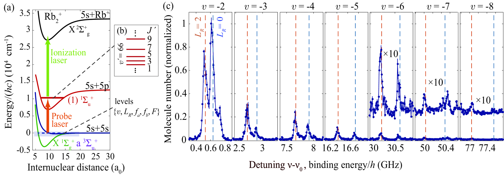
Figure 1: (a) Two-color REMPI scheme for state-selective detection of molecules. Probe and ionization lasers have a wavelength of $1065\>\textrm{nm}$ and $544\>\textrm{nm}$, respectively. (b) Rotational level structure of the relevant molecular states with negative parity. (c) Various segments of REMPI detection signals of ($\text{\char 118\relax},L_{R}=0,2$) product molecules as a function of the probe laser frequency $\nu$. Here, $\nu_{0}=281445.045\>\textrm{GHz}$, corresponding to the transition from the 5s 5s asymptote to $\text{\char 118\relax}^{\prime}=66,J^{\prime}=1$. The vibrational quantum numbers v are given on the top of the figure and the rotational quantum numbers $L_{R}$ are indicated by the color coding of the dashed vertical lines ($L_{R}=0$ and $2$ in blue and red, respectively). These dashed lines are expected frequency positions for the given states obtained from coupled-channel calculations. For smaller signals ($\text{\char 118\relax}=-6,-7,-8$) magnifications by a factor of 10 are also shown. The data for the most-weakly bound state $\text{\char 118\relax}=-1,L_{R}=0$ are not presented, because the corresponding line is largely drowned by a neighboring photoassociation line [11].

Our perturbative model indicates that for each angular momentum $L_{R}>0$ there is a critical binding energy $E_{c}(L_{R})$ so that for $E_{b}>E_{c}(L_{R})$ the trend of the partial recombination rate will be described by $L_{3}(E_{b},L_{R})=cE_{b}^{-\alpha}$, where $c$ is a constant. We find that the factor $c$ is roughly independent of $L_{R}$. For $E_{b}<E_{c}(L_{R})$ there is a suppression of $L_{3}(E_{b},L_{R})$ which can be explained as the effect of an angular momentum barrier in the exit channel. As a result, this suggests that only molecular states with small $L_{R}$ will significantly contribute to molecular production at low binding energies $E_{b}$.

Finally, we show that the $E_{b}^{-\alpha}$ scaling law can be also derived theoretically in an analytic, perturbative approach. We find that within this approach the $E_{b}^{-\alpha}$ scaling is quite independent on the long-range behavior of the interaction potential between two atoms. Specifically, potentials with a power law tail $-C_{n}/r^{n}$ for $n=3,4$ or 6, or the Morse potential, as well as the contact potential have $\alpha$-values in the range $[0.91,1]$.

Within the framework of the perturbative calculations the scaling of the rate constant $L_{3}(E_{b})$ is largely determined by $|\phi_{d}(\sqrt{E_{b}\,m/3})|^{2}$, where $\phi_{d}$ is the diatomic molecular wave function in momentum representation and $m$ is the atomic mass. It turns out that this part of the momentum wave function is linked to the molecular wave function in real space in the vicinity of the classical outer turning point of the molecular potential (at energy $-E_{b}$). This indicates that the outer classical turning point marks a typical distance for the recombination to occur.

II Experiment

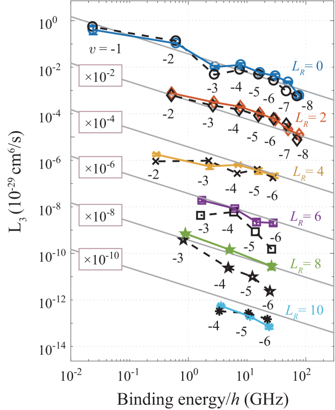
Figure 2: Measured (scaled) and calculated rate constants $L_{3}(\text{\char 118\relax},L_{R})$ for product molecules $(\text{\char 118\relax},L_{R})$ as a function of their binding energy $E_{b}$. The rotational quantum numbers $L_{R}$ are indicated by different plot symbols (black: calculations; colors: experiment). For each sequence of states with the same $L_{R}$ the vibrational quantum number v is given below the data points. For better visibility the data for each $L_{R}$ are shifted in vertical direction by multiplying them with $10^{-L_{R}}$. The gray solid lines show the energy scaling $(E_{b}/\textrm{GHz}\times h)^{-0.8}\times 0.2\times 10^{-29}\>\textrm{cm}^{6}/\textrm{s}$.

In our experiments we prepare an ultracold cloud of $5\times 10^{6}$ ⁸⁷Rb atoms in a far-detuned 1D optical lattice trap ($\lambda=1064\,$nm, trap depth $\approx 10\,\mu$K$\times k_{B}$) combined with an optical dipole trap so that we obtain a trap frequency of $2\pi\times 23$Hz in the transverse direction. The atoms are spin-polarized in the hyperfine state $f=1,m_{f}=-1$ of the electronic ground state and have a temperature of about $750\>\text{nK}$. Our measurements are carried out at a low external magnetic field of about $4\>\textrm{G}$. We hold the atom cloud in the trap for a duration of 500 ms during which Rb₂ molecules are spontaneously produced via three-body recombination in the coupled $X^{1}\Sigma_{g}^{+}-a^{3}\Sigma_{u}^{+}$ molecular complex, below the $5S_{1/2}+5S_{1/2}$ atomic asymptote. The molecules are state-selectively ionized via resonance-enhanced multiphoton ionization [REMPI] (see Fig. 1(a) and Appendix A for details), and then trapped and detected as ions in a Paul trap at a distance of 50 $\mu$m (see Appendix B for details). In brief, a first REMPI laser (the probe laser) resonantly excites such a molecule to the intermediate level $\text{\char 118\relax}^{\prime}=66,\,J^{\prime}$ of the state $A^{1}\Sigma_{u}^{+}$ using a wavelength of about 1065 nm [22, 23]. Here, $\text{\char 118\relax}^{\prime}$ is the vibrational quantum number and $J^{\prime}$ is the total angular momentum quantum number excluding nuclear spin. From the intermediate level a second laser (the ionization laser) at a wavelength of about 544 nm resonantly excites the molecule to a state above the Rb${}_{2}^{+}$ ionization threshold, so that the molecule can autoionize. In one experimental run we can detect and count up to $\approx$ 70 ions in the Paul trap. The ion number scales linearly with the molecule number. The corresponding scaling factor $\eta$ is the detection efficiency of a molecule. As discussed in Appendices A and C, $\eta$ is roughly constant over the range of bound states investigated in this work, and its value is $\eta\approx 4.8\times 10^{-3}$. A REMPI spectrum of a particular product state is obtained by scanning the probe laser frequency in steps of typically 5 MHz. Our setup features an improvement of the product state signals and the sensitivity by a factor of $\approx 25$ as compared to previous work [11], extending our detection range of binding energies to about $80\>\textrm{GHz}\times h$, which was instrumental for the present work (for details, see Appendix D).

In the following we specify molecular states by their vibrational quantum number v and their rotational quantum number $L_{R}$ only, which is sufficient due to the conservation of the hyperfine spin state in the reaction process [24]. Figure 1(c) shows product state spectra for molecules with $L_{R}=0$ or $2$, and with v ranging from $-2$ to $-8$. We note that whenever v is negative, it is counted downwards from the atomic $f_{a}=f_{b}=1$, $m_{fa}=m_{fb}=-1$ asymptote, starting with $\text{\char 118\relax}=-1$ for the most weakly bound vibrational level. The most deeply bound state, ($\text{\char 118\relax}=-8,L_{R}=0$), has a binding energy of $77\>\textrm{GHz}\times h$. Here, all signals are obtained using the same intermediate state $J^{\prime}=1$ for REMPI. The frequency reference $\nu_{0}$ corresponds to the photoassociation transition towards this intermediate state such that, at a resonance position, $(\nu-\nu_{0})\times h$ directly represents the binding energy of the initially produced molecular state. Our data clearly show that the production rate of molecules for a given rotational level $L_{R}$ generally drops with the binding energy $E_{b}$. The drop is significant over the investigated range of $E_{b}$. The relative strength of $L_{R}=0$ and $2$ signals, however, can vary for different vibrational levels v. Large molecular signals as, e.g., obtained for $\text{\char 118\relax}=-2$ correspond to 63(3) produced ions per run whereas typical background signals are 0.69(0.15) ions per run (see also Fig. 11 in Appendix D). In the measurements of Fig. 1(c) the number of repetitions of the experiment per data point was gradually increased from 5 to 40 for increasing binding energy, in order to improve the visibility of smaller signals. We assign the signals in our REMPI spectra by comparing their frequency positions to those obtained from close-coupled channel calculations (see, e.g., [11, 10]) and by observing characteristic rotational ladders, since any molecular state with $L_{R}>0$ can be detected via two different rotational states $J^{\prime}=|L_{R}\pm 1|$ [see Appendix E, not shown in Fig. 1(c)]. The deviations between calculated [dashed vertical lines in Fig. 1(c)] and measured resonance frequency positions are typically smaller than $\sim 30\>\textrm{MHz}$ and arise mainly from daily drifts of our wavelength meter.

III Quantitative analysis

We now carry out a quantitative analysis of the observed population distribution. Figure 2 shows measured (scaled) and calculated partial rate constants $L_{3}(E_{b})\equiv L_{3}(\text{\char 118\relax},L_{R})$ for the production of $(\text{\char 118\relax},\,L_{R})$ molecules at a temperature of 0.8$\>\mu$K. The experimental values for $L_{3}(\text{\char 118\relax},L_{R})$ were obtained by multiplying the measured ion numbers with a single calibration factor for all detected ($\text{\char 118\relax},L_{R}$) states. This factor was chosen to optimize the agreement between experiment and theory (Appendix C). As can be seen from Fig. 2, the theoretical predictions reproduce remarkably well the relative strengths of the state dependent rates $L_{3}(\text{\char 118\relax},L_{R})$ obtained from the experiments. The calculations are based on solving the three-body Schrödinger equation in an adiabatic hyperspherical representation [25, 18], using a single-spin model as described in Appendix F (see also Ref. [11]). Within our model the ⁸⁷Rb atoms interact via pairwise additive long-range van der Waals potentials with a scattering length of 100.36 a₀ [26]. The potentials are truncated and support $15$ $L_{R}=0$ molecular bound states, and a total of 240 bound states. We calculated the theory data point for $L_{R}=8$, $\text{\char 118\relax}=-3$ using a model potential with 12 $s$-wave bound states because for 15 $s$-wave bound states a numerical instability occurs specifically for this level.

Figure 2 reveals that the $L_{3}(\text{\char 118\relax},L_{R})$ rate roughly follows the overall scaling of $E_{b}^{-\alpha}$ for all rotational states. A fit analysis to the experimental data yields a scaling factor $\alpha={0.80(\pm 0.14)}$ (see gray solid lines), while the fit to the theoretical data yields $\alpha={0.77(\pm 0.10)}$. We point out that all gray solid lines in Fig. 2 correspond to exactly the same function, $(E_{b}/\textrm{GHz}\times h)^{-0.8}\times 0.2\times 10^{-29}\>\textrm{cm}^{6}/\textrm{s}$. For better visibility these lines along with the respective data points have been shifted in vertical direction by multiplying them with $10^{-L_{R}}$. We notice that the measured data for $L_{R}=2$ are all located above the gray line while the data for $L_{R}=4$ or $10$ are all below the gray line. This indicates that there is a systematic dependence of $L_{3}(E_{B})$ on $L_{R}$, as already discussed in [11]. Nevertheless, considering the overall range of $L_{3}$ and $L_{R}$ in our data, this variation of $L_{3}(E_{B})$ with $L_{R}$ is still comparatively small, typically within a factor of 2. Therefore, to a first approximation, the production rate does seem to be quite independent of the molecular rotation $L_{R}$. This fact might be somewhat counterintuitive given that the atoms initially collide with vanishing angular momenta and therefore products with small angular momenta would seem to be naturally preferable.

We note that there are considerable variations around the general $E_{b}^{-\alpha}$ scaling trend. For example, the rate for the state $\text{\char 118\relax}=-3,L_{R}=0$ is significantly lower than the rate for the more-deeply bound state $\text{\char 118\relax}=-4,L_{R}=0$. Remarkably, even such individual variations are largely reproduced by our numerical calculations. In general, the theoretical and experimental data curves are very similar, especially for the low rotational states $L_{R}=0$ and $L_{R}=2$. This suggests that our three-body model is quite accurate and that it should in principle be capable to track down how the deviations from the general scaling come about in individual cases. For example, we point to the experimental and theoretical data points for $\text{\char 118\relax}=-2$ and $L_{R}=4$, which are located below the $E_{b}^{-\alpha}$ scaling trend. This suppression may be due to an angular momentum barrier effect which we will discuss in Section V.2.

IV Perturbative approach

In order to gain a deeper insight into the observed energy scaling we discuss in the following a perturbative model for the partial three-body recombination rates $L_{3}(\text{\char 118\relax},L_{R})$. Generally, the rates $L_{3}(\text{\char 118\relax},L_{R})$ towards each specific molecular product $d=(\text{\char 118\relax},L_{R})$ are given by [27] (see also Appendix G)

$$L_{3}(\text{\char 118\relax},L_{R})=\frac{12\pi m}{\hbar}(2\pi\hbar)^{6}q_{d}|\langle\psi_{f}|U_{0}(E)|\psi_{\rm{in}}\rangle|^{2},$$ (1)

where $m$ represents the mass of an atom. $|\psi_{\rm{in}}\rangle$ is the initial state, consisting of three free atoms each propagating as a plane wave with essentially vanishing momentum. $|\psi_{f}\rangle$ is the final state of a free atom and a free molecule. Atom and molecule are asymptotically propagating as plane waves with relative momentum $q_{d}$ which is fixed by the molecular binding energy $E_{b}$ and the total energy $E$ of the three-body system via $\frac{3q_{d}^{2}}{4m}-E_{b}=E$, where we use the center of mass system as a reference. In Eq. (1), $U_{0}(E)$ represents a three-body transition operator which describes the transition process between the states. It can be approximated by a perturbative expansion (Appendix G) derived from the Alt-Grassberger-Sandhas (AGS) equation [28, 29, 27]. To the leading order of the expansion, we have a process where atoms $(a,b)$ of the three free atoms $(a,b,c)$ collide to exchange a momentum $\mathbf{q}_{d}$. During this collision atom $(b)$ is scattered into a molecular bound state with atom $(c)$. This is shown schematically in the inset of Fig. 3. The initial momenta of the atoms are 0. After the collision atom $(a)$ remains free and carries away the momentum $\mathbf{q}_{d}$ and a corresponding part of the released binding energy. The formed molecular bound state $\phi$ has a total momentum $-\mathbf{q}_{d}$ and the relative momentum between its atomic constituents is $(-\mathbf{q}_{d}/2)$. Apart from constants, the result of the calculation is

$$L_{3}(\text{\char 118\relax},L_{R})\propto q_{d}\,\,\,\left|\phi_{d}\left(\frac{1}{2}q_{d}\right)\right|^{2}\,\,\,|t_{\rm{h}}(q_{d})|^{2}.$$ (2)

Here, $\phi_{d}(p=\frac{1}{2}q_{d})$ corresponds to the radial part of the molecular wave function in momentum space. It is normalized according to $\int|\phi_{d}(p)|^{2}p^{2}dp=1$. The factor $t_{\rm{h}}(p^{\prime}=q_{d})\equiv$ $\langle p^{\prime}=q_{d}|t^{s}(0)|p=0\rangle$ is the matrix element of the $s$-wave component $t^{s}$ of the two-body transition operator $t$ for the two-body collision and we have set $E=0$. Here, $p$ ($p^{\prime}$) represent the relative momenta of the incoming (outgoing) two colliding atoms, respectively. Within the perturbative approximation, the $E_{b}$ scaling of $L_{3}(\text{\char 118\relax},L_{R})$ can only result from two-body quantities, i.e., $E_{b}$, $\phi_{d}$ and $t_{\rm{h}}$. Since $E\approx 0$, one obtains $q_{d}\approx 2\sqrt{E_{b}\,m/3}$.

In order to analyze the scaling of $L_{3}(\text{\char 118\relax},L_{R})$ with the molecular binding energy $E_{b}$, we discuss $\phi_{d}(\sqrt{E_{b}\,m/3})$ and $t_{\rm{h}}(2\sqrt{E_{b}\,m/3})$ separately. We find that $t_{\rm{h}}(p)$ oscillates but its amplitude varies only gently with $p$ until the deeply-bound states are reached (see Fig. 13(a) in Appendix G). Therefore, $t_{\rm{h}}(2\sqrt{E_{b}\,m/3})$ cannot strongly contribute to an overall scaling with $E_{b}$ for the three-body recombination rate. In contrast to that, $\phi_{d}(\sqrt{E_{b}\,m/3})$ which is obtained from two-body bound state calculations, vanishes quickly with increasing $E_{b}$. This is shown in Fig. 3 (yellow data points) for atoms interacting via the van der Waals potential. Besides the overall decrease of $|\phi_{d}(\sqrt{E_{b}\,m/3})|^{2}$ for growing $E_{b}$, there are also oscillations. The sharp drops in these oscillations correspond to the nodes of the various momentum wave functions $\phi_{d}$ for the bound states with energy $E_{b}$. While the oscillations lead to some scatter of the data, the upper envelope of the data points indicates an overall power law scaling of the amplitude. A fit to this envelope (dotted line in Fig. 3) gives $|\phi_{d}(\sqrt{E_{b}\,m/3})|^{2}\propto E_{b}^{-1.44\pm 0.03}$ which yields $L_{3}\propto E_{b}^{-0.94\pm 0.03}$. This result agrees quite well with our full calculations from Fig. 2. We note that in the shown energy range there are only 13 bound states in the van der Waals potential, resulting in 13 data points. In order to map out in more detail the functional form of $|\phi_{d}(\sqrt{E_{b}\,m/3})|^{2}$ in Fig. 3 we have slightly varied $\lambda_{6}$ over four different values (while keeping the number of bound states in the potential constant). The variation in $\lambda_{6}$ leads to variations of $E_{b}$ and therefore also of $\phi_{d}$ and the scattering length $a$. When we present all these data points together, a quasi-continuous curve is obtained. We note that the oscillating amplitude of $t_{\rm{h}}(p)$, which is nearly constant for a fixed scattering length $a$, can depend on $a$.

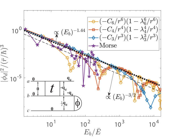
Figure 3: Plot of $|\phi_{d}(\sqrt{E_{b}\,m/3})|^{2}\propto L_{3}(E_{b})/\sqrt{E_{b}}$ versus $E_{b}$ for various two-body potentials. These are the potentials with the power-law tail, $\sim-C_{n}/r^{n}$ for $n=3,4$ or 6, and the Morse potential $D_{e}[e^{-2a(r-r_{e})}-2e^{-a(r-r_{e})}]$ (see legend). We use $\bar{E}=\hbar/m\bar{r}^{2}$, with $\bar{r}=\frac{1}{2}(mC_{n}/\hbar^{2})^{1/(n-2)}$ for the power-law potentials and $\bar{r}=a$ for the Morse potential, respectively. The values for $\lambda_{n}$ and $D_{e}$ are chosen such that the potentials have 14 or 15 $s$-wave bound states. The shown points correspond to bound states with $\text{\char 118\relax}\geq-13$. In order to map out the function $|\phi_{d}(\sqrt{E_{b}\,m/3})|^{2}$ better we show data points for four different values for $\lambda_{n}$ (for each $n$) or for $D_{e}$ (see text). The dotted line is a power-law fit to the upper envelope of the data points for the $-C_{6}/r^{6}$ potential as well as the other potentials. The dashed line represents the scaling for contact interactions. For $n=6$ the energy range considered in this figure corresponds to [0.01 …100] GHz$\times h$ for ⁸⁷Rb atoms. The inset describes the scattering process in the perturbative approximation (see Appendix G). Horizontal lines represent atoms and the numbers above these lines denote single atom momenta. The relative momentum between two atoms is indicated by a number that connects to the corresponding horizontal lines by arrows.

V Energy scaling for general long-range potentials

Remarkably, we find that the scaling law is similar for a range of different two-body interaction potentials, such as the Morse potential and potentials of the form $V(r)=-C_{n}/r^{n}(1-\lambda_{n}^{n}/r^{n})$. Here, the parameter $n$ is typically $n=3,4$ or 6, and $\lambda_{n}$ is a short-range parameter which defines the inner barrier. The case $n=6$ corresponds to the Lennard-Jones potential which was already discussed in the previous section. The corresponding functions $|\phi_{d}(\sqrt{E_{b}\,m/3})|^{2}$ are shown in Fig. 3. Clearly, their envelopes roughly decrease in a similar manner, i.e. $\approx E_{b}^{-1.44\pm 0.03}$. Furthermore, we also consider contact interactions between the atoms. For these, we use $\phi_{d}(p)=\frac{2}{\sqrt{\pi}}\frac{(m\,E_{b})^{1/4}}{p^{2}+m\,E_{b}}$ and analytically obtain from Eq. (2) the scaling to be exactly $|\phi_{d}(\sqrt{E_{b}\,m/3})|^{2}\propto 1/E_{b}^{3/2}$ (see black dashed line in Fig. 3), corresponding to $L_{3}(E_{b})\propto 1/E_{b}$. Therefore, even the results for contact interaction are in relatively good agreement with our other numerical and the experimental results.

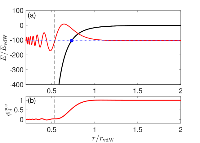
Figure 4: (a) Typical example for a molecular wave function (red solid line) located in the $-C_{6}/r^{6}$ van der Waals potential (black solid line). The blue horizontal dotted line and the blue circle indicate the molecular level position $-E_{b}$ and the corresponding classical outer turning point, respectively. The vertical dashed line shows the starting position of the last lobe of the molecular wave function. (b) shows the accumulated Fourier integral $\phi^{\rm{acc}}_{d}(\sqrt{mE_{b}/3};r)$, see text. $E_{\mathrm{vdW}}=\hbar/mr_{\mathrm{vdW}}^{2}$ is the van der Waals energy and $r_{\mathrm{vdW}}=\frac{1}{2}(mC_{6}/\hbar^{2})^{1/4}$ is the van der Waals length.

In the following we discuss how this similar scaling for the different long-range potentials can be explained. We make use of approximate analytical wave functions for the molecular bound state. Let $\psi(r)=u(r)/r$ be the radial part of the molecular wave function with rotational angular momentum $L_{R}$. Here, $r$ is the internuclear distance between the two atoms. A typical example of the reduced radial wave function $u(r)$ is shown in Fig. 4(a). The Fourier transform of $u(r)/r$ generates the molecular wave function in momentum space

$$\phi_{d}(p) = \sqrt{\frac{2}{\pi}}\int_{0}^{\infty}rj_{L_{R}}(pr/\hbar){u}(r)dr,$$ (3)

where $j_{L_{R}}$ is the spherical Bessel function of the first kind of order $L_{R}$. A numerical analysis shows that the dominant contribution to $\phi_{d}(\sqrt{E_{b}m/3})$ comes from the last lobe of $u(r)$, which is located around the classical outer turning point $r_{0}$. In Fig. 4(b) we show the Fourier integral for the case $L_{R}=0$ in an accumulated fashion $\phi^{\rm{acc}}(p;r)=\int_{0}^{r}\sin(pr/\hbar)u(r)dr/\int_{0}^{\infty}\sin(pr/\hbar)u(r)dr$, which verifies the dominant contribution of the last lobe. The turning point of the level [blue circle in Fig. 4(a)] is determined by $\tilde{V}(r_{0})+E_{b}=0$, where $\tilde{V}(r)=V(r)+\hbar^{2}L_{R}(L_{R}+1)/(mr^{2})$. The reduced radial wave function $u(r)=r\psi(r)$ in this region is approximated by $\tilde{u}(r)=\mathcal{N}^{1/2}\textrm{Ai}[s(r-r_{0})]$, where Ai($x$) is the Airy function, $s=(mD/\hbar^{2})^{1/3}$, $D=d\tilde{V}(r)/dr|_{r=r_{0}}$, and $\mathcal{N}$ is a normalization factor that ensures that $\tilde{u}(r)$ best matches $u(r)$ in the region. It turns out that to a good approximation $\mathcal{N}=sN$, where $N$ is a constant independent of $E_{b}$ [30]. We Fourier transform $\tilde{u}(r)$ and obtain

$$\tilde{\phi}_{d}(p) = \sqrt{\frac{2N\hbar^{2}}{\pi sp^{2}}}g_{d}(p)\,,$$ (4)

where

$$g_{d}(p)=\int_{0}^{\infty}\frac{p\tilde{r}}{s\hbar}j_{L_{R}}(p\tilde{r}/s\hbar)\textrm{Ai}(\tilde{r}-\tilde{r}_{0})d\tilde{r}.$$ (5)

Here, $\tilde{r}=sr$, $\tilde{r}_{0}=sr_{0}$. At $p=\sqrt{E_{b}m/3}$, we get

$$|\tilde{\phi}_{d}(\sqrt{E_{b}m/3})|^{2} =\frac{6N\hbar^{2}}{\pi smE_{b}}g_{d}^{2}(\sqrt{E_{b}m/3}),$$ (6)

which approximates $|\phi_{d}(\sqrt{E_{b}m/3})|^{2}$.

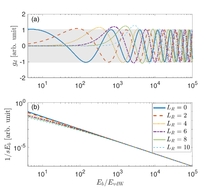
Figure 5: (a) Plot of $g_{d}(\sqrt{E_{b}m/3})$ as a function of $E_{b}$ for the partial waves $L_{R}\leq 10$ (see legend in (b)). The gray area highlights the range of the oscillation for $L_{R}=0$. (b) Plot of $1/(sE_{b})$. For both (a) and (b) we use the $-C_{6}/r^{6}$ potential.

After this general discussion we now discuss the cases for $L_{R}=0$ and $L_{R}>0$.

V.1 Case: $L_{R}=0$

For a $L_{R}=0$ molecular state and $\tilde{V}(r)=-C_{n}/r^{n}$ the classical outer turning point is given by $r_{0}=(C_{n}/E_{b})^{1/n}$. From the derivative of the potential $\tilde{V}(r)$ we obtain for the parameter $s$ (which we defined earlier in connection with the Airy function),

$$s =(mn/\hbar^{2})^{1/3}E_{b}^{(n+1)/3n}C_{n}^{-1/3n}.$$ (7)

Thus, the factor $6N\hbar^{2}/(\pi smE_{b})$ in Eq. (6) scales as $E_{b}^{-(4n+1)/3n}$. The other factor in Eq. (6), $g_{d}(\sqrt{E_{b}m/3})$, is plotted in Fig. 5(a) for $n=6$, (blue line). $g_{d}(\sqrt{E_{b}m/3})$ oscillates between 1 and -1 with a constant amplitude, as indicated by the gray area. Therefore, $g_{d}(\sqrt{E_{b}m/3})$ does not contribute to an overall scaling of $|\phi_{d}(\sqrt{E_{b}m/3})|^{2}$ with $E_{b}$. This is similar as for $t_{h}(q_{d})$ as mentioned in Sec. IV. The variation of $g_{d}(\sqrt{E_{b}m/3})$ merely leads to some scatter of $L_{3}$. Therefore, we ignore $g_{d}(\sqrt{E_{b}m/3})$ in the following discussion on scaling and obtain,

$$|\phi_{d}(\sqrt{E_{b}m/3})|^{2}\propto E_{b}^{-(4n+1)/3n}=E_{b}^{-\beta}.$$ (8)

For $n=3,4$ and 6, the exponent $\beta=(4n+1)/3n$ takes the values of 1.44, 1.42 and 1.39, which agree very well with our numerical results in the perturbative approach. For the scaling of $L_{3}$ we have $L_{3}\propto E_{b}^{-\alpha}$, where $\alpha=\beta-0.5$ . It is remarkable that for any positive integer $n$ the exponents are constrained to a narrow range, i.e. $\beta\in$ [1.33, 1.67] and $\alpha\in$ [0.83, 1.17]. Considering that a real interaction potential can typically be expanded in terms of the $-C_{n}/r^{n}$ functions, these ranges should be valid quite generally. In fact, the range of $\alpha\in$ [0.83, 1.17] agrees with the exponent $\alpha=0.8\pm 0.14$ extracted from our experimental measurements within the range of uncertainty.

V.2 Case: $L_{R}>0$

We now consider the case of rotational angular momentum $L_{R}>0$. Because for this case we do not obtain a simple analytical expression for $s$ as in Eq. (7), we only present numerical results. Figure 5(b) shows a plot of $1/(sE_{b})$ for various $L_{R}$ (and using the $-C_{6}/r^{6}$ potential as a typical example). Clearly, all curves are quite similar, especially for large $E_{b}$. The functions $g_{d}(\sqrt{E_{b}m/3})$ are shown in Fig. 5(a), as discussed before. They oscillate with a constant amplitude and therefore do not contribute to the energy scaling for large energies $E_{b}$. As a consequence, the energy scaling is quite independent on the rotational state $L_{R}$ of the molecule. Figure 6 shows calculations for $|\phi_{d}(\sqrt{E_{b}\,m/3})|^{2}$ for various rotational angular momenta of the molecule. As a typical example we use the Lennard-Jones potential. Similar as for Fig.3 we have slightly varied $\lambda_{6}$ over four different values in order to increase the number of data points and to better map out $|\phi_{d}(\sqrt{E_{b}\,m/3})|^{2}$. The sudden drops in $|\phi_{d}(\sqrt{E_{b}\,m/3})|^{2}$ reflect nodes of the molecular wave function. For large enough binding energy $E_{b}$ all curves for the different values of $L_{R}$ follow the same power law $E_{b}^{-1.45}$ corresponding to an energy scaling of the partial rate constants (for fixed $L_{R}$) of $L_{3}(E_{b})\propto E_{b}^{-0.95}$.

We note, however, that for $L_{R}>0$ and small enough binding energies, our calculations in Fig. 6 reveal a strong suppression of $|\phi_{d}|^{2}$ and therefore of $L_{3}(E_{b})$. This effect is due to the function $g_{d}(\sqrt{E_{b}m/3})$. As shown in Fig. 5 (a), for $L_{R}>0$, $g_{d}(\sqrt{E_{b}m/3})$ increases gradually with $E_{b}$ starting from 0. When it reaches its first maximum, it goes over to the previously discussed oscillatory behavior in the gray area, similar to the case of $L_{R}=0$. As a consequence, $|\phi_{d}(\sqrt{E_{b}m/3})|^{2}$ is increasingly suppressed for $E_{b}\rightarrow 0$, as observed in our numerical results. This suppression can be understood as an effect of the angular momentum barrier. In a simple picture, in order to create a molecule rotating with angular momentum $L_{R}$ at interparticle distance $r_{0}$ of the outer turning point, a minimal momentum $p_{c}$ needs to be supplied of the order $p_{c}\approx\hbar L_{R}/r_{0}$. The minimal momentum $p_{c}$ translates into a minimal binding energy $E_{c}=3p_{c}^{2}/m\approx\hbar^{2}L_{R}(L_{R}+1)/(mr_{0}^{2})$. At the same time we have $E_{c}\approx C_{6}/r_{0}^{6}-\hbar^{2}L_{R}(L_{R}+1)/(mr_{0}^{2})$. Combining these two equations to eliminate $r_{0}$ one can estimate the critical energy $E_{c}$ to be

$$E_{c}/E_{\rm{vdW}}\approx c_{c}\left[L_{R}(L_{R}+1)\right]^{3/2},$$ (9)

where $c_{c}=1.5$ and $E_{\rm{vdW}}=4\hbar^{3}/(m^{3/2}C_{6}^{1/2})$ is the van der Waals energy. Reading off $E_{c}(L_{R})$ from our numerical results in Fig. 6 as the first maximum of $|\phi_{d}(\sqrt{E_{b}m/3})|^{2}$ we find that the data points are well described by Eq.(9) when we use $c_{c}=2.12$, see inset of Fig. 6. This validates our simple interpretation of the angular momentum suppression.

VI Discussion

We now compare and discuss the results of our theoretical and experimental approaches. The suppression effect for large $L_{R}$ and small $E_{b}$, which is so clearly visible in Fig. 6 is not so obvious in Fig. 2 where we present our experimental data and our full coupled channel calculations. A small suppression effect might only be recognizable for the state $\text{\char 118\relax}=-2,L_{R}=4$ in Fig. 2. In practice, the observation of suppressed low-energy high-$L_{R}$ molecular signals can be hampered by various issues. By accident it can occur that no weakly-bound molecular level with $E_{b}<E_{c}$ exists for a given rotational angular momentum $L_{R}$. In fact, quantum defect theory predicts for a van der Waals potential that if the most weakly-bound state for a partial wave $L_{R}$ is not close to threshold, then also the most weakly-bound state for the partial wave $L_{R}+4$ will not [31]. Alternatively, the level can be overlooked experimentally, if its signal is too weak. It will be overlooked theoretically if the level has a vibrational quantum number beyond the limits of the model potential. It should be, however, clear that the suppression mechanism must exist. Indeed, in a recent experiment on diatomic molecular reactions, a similar suppression mechanism has been identified [14].

When comparing Fig. 6 with Fig. 2 it is evident that the distinct drops of $|\phi_{d}(\sqrt{E_{b}m/3})|^{2}$ in Fig. 6 do not clearly appear in Fig. 2. There are several possible explanations for this. First, the data sampling in Fig. 2 is seven times smaller than for Fig. 6. Therefore, it is likely that a narrow drop is not encountered in Fig. 2. Second, the calculations in Fig. 6 correspond to the leading order of an expansion. Including higher orders might wash out the sudden drops, as other pathways for the molecular formation can be taken.

Concerning the full model and the experiment, we expect that the scaling exponent $\alpha$ of the $E_{b}^{-\alpha}$ scaling law is prone to changes for deeper binding energies than the ones considered here. As recently discussed in [10], for ⁸⁷Rb and $E_{b}>150\>\textrm{GHz}\times h$ the spin conservation propensity rule which allows for working with a single spin channel should break down, affecting the scaling law. In addition, the short-range three-body interaction, which is ignored so far in our treatment, should play an increasingly important role when forming more tightly bound molecular states. Recent work on three-body recombination of hydrogen [20] has already found evidence for this, as the Jahn-Teller effect substantially enhances recombination rates into tightly bound molecular states.

Figure 6: Powerlaw scaling of $|\phi_{d}(\sqrt{E_{b}\,m/3})|^{2}\propto L_{3}(E_{b})/\sqrt{E_{b}}$ for various rotational angular momenta $L_{R}$. The data points are a full calculation for the Lennard-Jones potential $(-C_{6}/r^{6})(1-\lambda_{6}^{6}/r^{6})$. As in Fig.3 and Section IV, we have slightly varied $\lambda_{6}$ over seven different values while keeping the number of bound states in the potential constant. This helps to map out $|\phi_{d}(\sqrt{E_{b}\,m/3})|^{2}$ in detail. Therefore, although there are only 8 bound states in the shown energy range we obtain 55 data points. The solid lines are calculations for the Lennard-Jones potential using Eq. (6). The dashed lines show the $E_{b}^{-1.45}$ energy scaling for $|\phi_{d}|^{2}$, as determind by a fit to the upper envelope of the data set. For better visibility the data for $L_{R}>0$ are shifted in vertical direction by multiplying them with $10^{-L_{R}}$. We define $E_{c}$ to be the energy at which the curve $|\phi_{d}|^{2}$ (for a given $L_{R}$) has its first maximum (coming from low energy). The inset shows $E_{c}$ as a function of $L_{R}$ (diamonds). The data are well described by Eq. (9) (solid line).

VII Summary and Outlook

To summarize, we have experimentally and theoretically investigated how the three-body recombination of an ultracold gas scales with the molecular binding energy $E_{b}$, detecting bound levels from 0.02 to 77 GHz $\times h$, thus spanning an energy range of more than three orders of magnitude. This became possible by applying improved experimental schemes for the state-to-state detection of molecules and by carrying out large scale numerical calculations. Besides these numerical calculations an analytical perturbative model was developed which gives deep physical insights into the recombination process and can explain the observed scaling law. In particular, the perturbative model shows that to a large part the scaling law can be extracted from two-body quantities such as the molecular wave function. Our experimental and theoretical approaches show that the three-body recombination exhibits a propensity towards weakly bound product molecules. The recombination rate follows a $E_{b}^{-\alpha}$ scaling law where $\alpha$ is in the vicinity of 1. Remarkably, we find that this scaling law is quite universal as it should hold for a range of different potentials such as the Morse potential, potentials of type $-C_{n}/r^{n}$ with $n=3,4,6$, as well as the contact potential. In addition, apart from a centrifugal barrier suppression at low enough binding energies, our results indicate that the three-body recombination populates molecular quantum states with different rotational angular momenta quite evenly, within about a factor of two.

In the future it will be interesting to explore how the scaling law evolves for deeper binding energies and what physical mechanisms will lead to its breakdown. On the experimental side, the detection sensitivity must be enhanced and the spectroscopic data will be expanded for reliable quantum state identification. On the theory side, short-range three-body interactions which are ignored so far in our treatment will be taken into account.

Moreover, it will be insightful to explore how deviations of individual reaction channels from the $E_{b}^{-\alpha}$ scaling law can be explained on a microscopic level, e.g. as interference effects of collision pathways. In fact, our perturbative calculations already produce tell-tale oscillations and it will be interesting whether we can match up these oscillations with the ones from the hyperspherical approach. This might give deeper insights into the reaction process.

We expect that our results on the scaling of the reaction rate with energy are not restricted to the recombination process of neutral atoms alone, but they can also be applied to other systems and processes. For example, these systems could involve molecules or ions as collision partners and they might also comprise a range of collisional relaxation processes. We expect these process rates to be governed by a $E_{b}^{-\alpha}$ scaling law, where $\alpha$ should always be in the vicinity of unity.

APPENDIX A The (1,1) REMPI

Our (1,1) REMPI scheme consists of two excitation steps which are described in the following. The overall ionization efficiency $\eta$ is given by the product of the efficiencies of the first and the second (1,1) REMPI step. We achieve $\eta\approx 4.8\times 10^{-3}$ (see also Appendix C) for all ($\text{\char 118\relax},L_{R}$) product molecules that we probe in the experiment. This is about an order of magnitude larger as compared to our previous work [11, 12].

A.1 First REMPI step

The first REMPI step resonantly excites a molecule towards the intermediate level $\text{\char 118\relax}^{\prime}=66,\,J^{\prime}$ of the state $A^{1}\Sigma_{u}^{+}$ using a wavelength of about 1065 nm [22, 23]. For this excitation we use a cw external-cavity diode laser with a short-term linewidth of about $100\>\text{kHz}$. It has a waist ($1/e^{2}$-radius) of $\approx 280\>\upmu\text{m}$ and an intensity of $\approx 12\>\text{W}\,\text{cm}^{-2}$ at the position of the atomic cloud. The laser is frequency-stabilized to a wavelength meter achieving a shot-to-shot and long-term stability of a few megahertz. The laser beam polarization has an angle of about 45^∘ with respect to the $B$-field and can therefore drive $\sigma$- and $\pi$-transitions.

We estimate that the first REMPI step is saturated for the molecular states considered in this work. This means a molecule is resonantly excited to the intermediate level $J^{\prime}$ with nearly unit probability when probed. In order to derive this we consider the following quantities: The transition electric dipole moment, the limited time to optically excite the product molecule, and a detuning due to the Doppler shift. In Fig. 7 we show calculated squared reduced transition electric dipole moments $D^{2}$ for transitions from ($\text{\char 118\relax},\,L_{R}$) product states towards the vibrational level $\text{\char 118\relax}^{\prime}=66$ within $A^{1}\Sigma_{u}^{+}$ (green columns). For convenience, $D^{2}$ is normalized by a global factor so that its value for ($\text{\char 118\relax}=-2,L_{R}=0$) equals to 1. As a general pattern, $D^{2}$ increases with binding energy in the range between the threshold and the vibrational quantum number $\text{\char 118\relax}=-9$. This is, however, partially compensated by the following kinetic effects. In the formation of the molecule by three-body recombination the binding energy is converted into kinetic energy of the products. Neglecting the energy of the ultracold atoms, the velocity $\text{\char 118\relax}_{\mathrm{Rb2}}$ of the molecule is $\propto E_{b}^{1/2}$. This velocity has two effects. First, it limits the time scale $\propto 1/E_{b}^{1/2}$ for the molecule to be located in the detection region, as determined by the size of the REMPI laser beams. Second, the velocity will on average lead to Doppler-broadening and to a reduction of the on-resonance photoexcitation rate by a factor given by $f_{D}=(2v_{\mathrm{Rb2}}/(\lambda\gamma))^{-1}\arctan(2v_{\mathrm{Rb2}}/(\lambda\gamma))$, where $\lambda$ is the transition wavelength and $\gamma\approx 2\pi\times 15\text{MHz}$ is the linewidth of the excited state. Therefore, the optical excitation probability $K_{I}$ of the molecules approximately scales as $K_{I}\propto D^{2}f_{D}/E_{b}^{1/2}$. In Fig. 7 we plot $K_{I}$ which is also normalized so that for $(\text{\char 118\relax}=-2,L_{R}=0)$ it equals to 1 (blue columns). Again, down to $\text{\char 118\relax}=-9$ there is a tendency that the ionization efficiency increases for increasing binding energy. In [11] we have found that for the given parameters of the probe laser beam the transitions from $\text{\char 118\relax}=-2,\,L_{R}=0,\,2$ towards the intermediate state are driven in a strongly saturated regime. Since all transitions for the product molecules in Fig. 7 have a $K_{I}$ close or larger than the ones for $\text{\char 118\relax}=-2,\,L_{R}=0,\,2$, we can expect saturation of the first step of the (1,1) REMPI for all considered product levels.

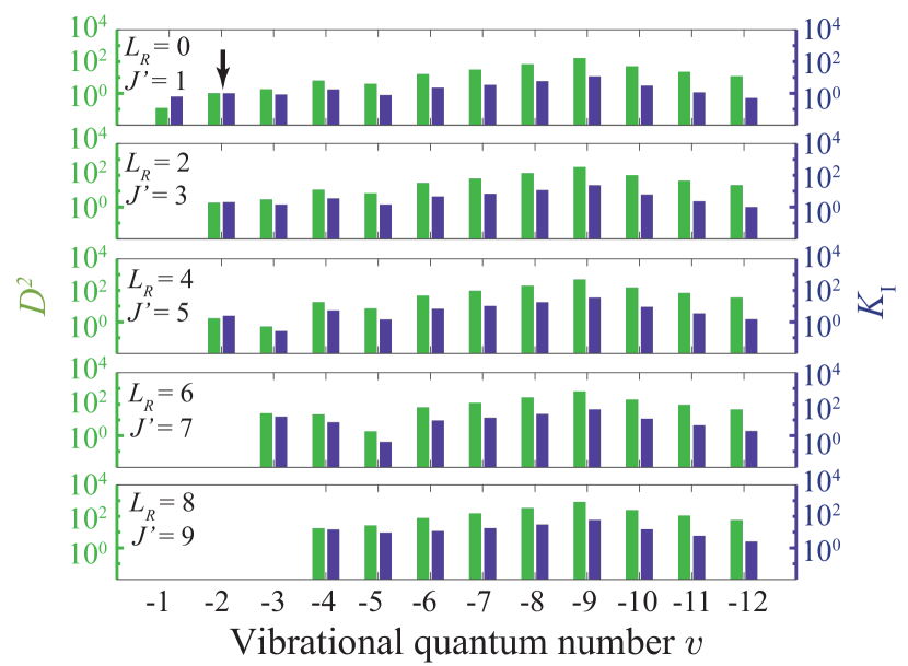
Figure 7: Calculations for the squared reduced transition electric dipole moment $D^{2}$ and relative transition probability $K_{I}\propto D^{2}f_{D}/E_{b}^{1/2}$ for the transitions from the product states ($\text{\char 118\relax},L_{R}$) towards the intermediate states $J^{\prime},\,\text{\char 118\relax}^{\prime}=66$ of $A^{1}\Sigma_{u}^{+}$. Both, $D^{2}$ and $K_{I}$ are normalized by a global factor, respectively, so that their values for the state $\text{\char 118\relax}=-2,\,L_{R}=0$ are 1 (see arrow). The plot is logarithmic.

A.2 Second REMPI step

For the second step of the REMPI we use the ionization laser at 544 nm to resonantly drive a transition from the intermediate state to a probably autoionizing molecular Rb₂ level [see Fig.  1(a)]. The laser is a cw, frequency-doubled OPO system from Hübner Photonics. It has a short-term linewidth on the order of $1\>\text{MHz}$. At the position of the atomic cloud the beam waist is $240\>\upmu\text{m}$ and we typically work with an intensity of $110\>\text{W}\,\text{cm}^{-2}$. As the probe laser, it is frequency-stabilized to a wavelength meter achieving a shot-to-shot and long-term stability of a few megahertz. The laser polarization is at an angle of about 45^∘ with respect to the $B$-field and can therefore drive $\sigma$- and $\pi$-transitions. When the excited Rb₂ molecule autoionizes it produces a deeply bound Rb${}_{2}^{+}$ molecular ion. Figure 8 shows resonance lines when scanning the frequency $\nu_{I}$ of the ionization laser and starting from the intermediate state $A^{1}\Sigma_{u}^{+},\,\text{\char 118\relax}^{\prime}=66,\,J^{\prime}=1$ which has been populated via photoassociation. These lines are spectroscopically not yet assigned. For REMPI via $J^{\prime}=1$ we use the resonance line centered at $\nu_{I}=\nu_{\mathrm{res}}=551422.660\>\textrm{GHz}$ (marked by an arrow).

Regarding the intermediate states with $J^{\prime}>1$, we carry out similar spectroscopy as for Fig. 8 and identify the strongest resonance, respectively, which is then used for REMPI. Since photoassociation cannot produce a molecule with $J^{\prime}>1$ in our cold sample, we instead populate such a state by resonantly exciting suitable product molecules ($\text{\char 118\relax},L_{R}$) after three-body recombination with the probe laser. Table 1 lists the optimal ionization laser frequencies for various rotational levels $J^{\prime}$ of the intermediate state $\text{\char 118\relax}^{\prime}=66$. From additional spectroscopic measurements we extract a rotational constant $B_{\text{\char 118\relax}^{\prime}=66}=443(2)\>\text{MHz}\times h$, in agreement with the value reported in [23]. For completeness, we present in Table 1 also the measured level energies $E_{J^{\prime}}$ for the various detected rotational states $J^{\prime}$ within $\text{\char 118\relax}^{\prime}=66$ of $A^{1}\Sigma_{u}^{+}$.

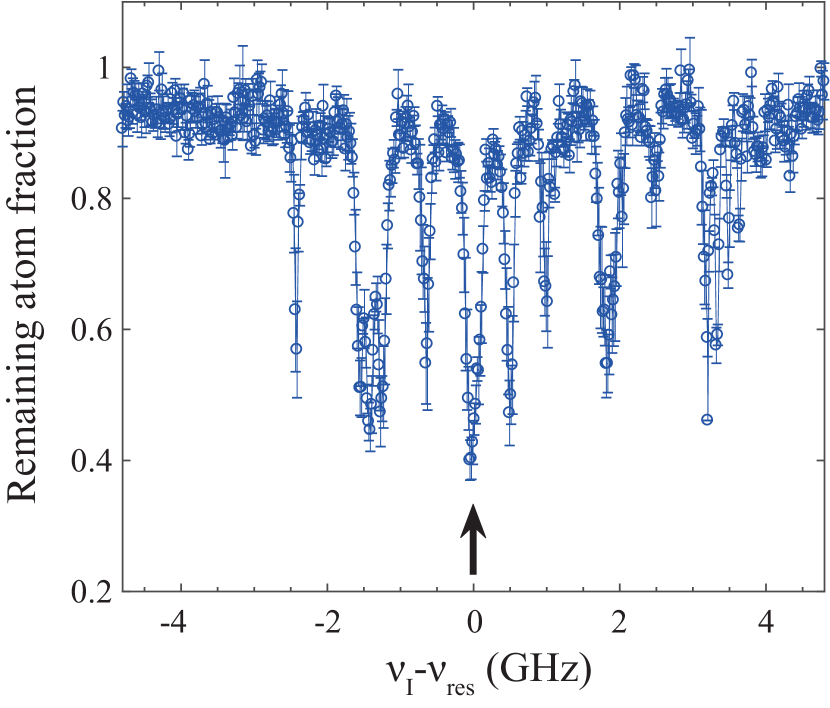
Figure 8: Resonance spectrum when scanning the frequency $\nu_{I}$ of the ionization laser, starting from the intermediate level $A^{1}\Sigma_{u}^{+},\,\text{\char 118\relax}^{\prime}=66,\,J^{\prime}=1$. Here, produced ions are detected by induced loss in an atom cloud (see Appendix B). The strongest line is marked by an arrow and has the center frequency $\nu_{\mathrm{res}}=551422.660\>\textrm{GHz}$.

$J^{\prime}$	$E_{J^{\prime}}$	$\nu_{\mathrm{res}}$
	$\textrm{GHz}\times h$	GHz
1	281,445.045	551,422.66
3	281,449.481	551,420.70
5	281,457.442	551,419.30
7	281,468.987	551,423.10
9	281,484.065	551,421.60

Table 1: REMPI paths. Column two lists the energies $E_{J^{\prime}}$ of the intermediate levels $J^{\prime}$ in the state $\text{\char 118\relax}^{\prime}=66$ of $A^{1}\Sigma_{u}^{+}$, with respect to the $(5s,f=1)+(5s,f=1)$ atomic asymptote. In the third column we list the frequencies $\nu_{\mathrm{res}}$ of the ionization laser which are used in the (1,1) REMPI scheme for the second transition starting from the intermediate levels $J^{\prime}=1,3,5,7,9$ in the state $\text{\char 118\relax}^{\prime}=66$ of $A^{1}\Sigma_{u}^{+}$.

The second REMPI step is generally not saturated in our experiment. This is shown in Fig. 9 for the case of initial ($\text{\char 118\relax}=-2,L_{R}=2$) molecules and the intermediate level $J^{\prime}=1$, $\text{\char 118\relax}^{\prime}=66$ of $A^{1}\Sigma_{u}^{+}$. The detected number of ions increases linearly with laser intensity. We have, however, verified that ionization of a given initial state via different intermediate rotational states $J^{\prime}=L_{R}\pm 1$ provides similar ion signal strengths. Furthermore, the reduction $f_{D}$ due to the Doppler effect (as discussed for the REMPI step 1) should be negligible here, since the linewidth $\gamma$ is about $200\>\textrm{MHz}$ according to Fig. 8. We note that $\gamma$ corresponds to an approximate measure of the autoionization width.

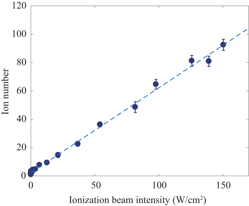
Figure 9: Ion number as a function of the intensity of the ionization laser beam in the (1,1) REMPI scheme. These data are obtained for ($\text{\char 118\relax}=-2,L_{R}=2$) molecules which are ionized via the intermediate state $J^{\prime}=1$. Here, $\nu_{I}=551,422.66\>\textrm{GHz}$, see Table 1. The dashed blue line is a linear fit to the data.

APPENDIX B Counting REMPI ions via atom loss

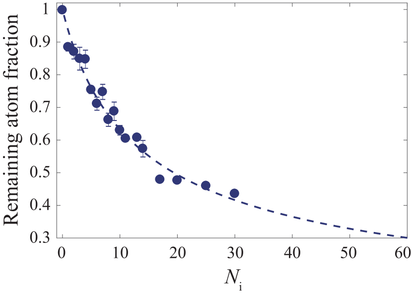
Figure 10: Remaining atom fraction as a function of the initially prepared number of ions $N_{i}$ (Rb⁺ and Rb${}_{2}^{+}$) after an interaction time of $500\>\textrm{ms}$. The dashed line is a fit of the function $(\frac{N_{\text{i}}}{c_{1}}+1)^{c_{2}}$ to the data (see text).

We detect and count ions in the Paul trap via atom loss which the ions inflict on neutral atoms due to elastic atom-ion collisions. The basic method has been developed in previous work [32, 6, 11]. Here, we use a modified scheme, which is described in the following.

Ion-inflicted atom loss: After the 500 ms phase of three-body recombination, the REMPI lasers are switched off and the optical lattice trap with the atom cloud is adiabatically moved over a distance of $50\>\mu\textrm{m}$ to the center of the Paul trap, in order to immerse the ions which have been produced during the 500 ms time into the atom cloud. At the same time the optical lattice trap is adiabatically converted into a crossed dipole trap, by turning off one of the 1D lattice beams. The trap frequencies of the crossed optical dipole trap are $\omega_{x,\,y,\,z}=2\pi\times(23,\,180,\,178)\>\text{Hz}$, where $z$ represents the vertical direction. In this trap the atom cloud is Gaussian-shaped with widths of $\sigma_{x,\,y,\,z}\approx(58.6,\,7.5,\,7.5)\>\upmu\text{m}$ and it still consists of about $4\times 10^{6}$ atoms, corresponding to a peak atomic density of about $n_{0}=0.9\times 10^{14}\>\text{cm}^{-3}$. In the Paul trap the ions have typical kinetic energies on the order of $\text{mK}\times k_{B}$ or larger as a result of, e.g., excess micromotion. Therefore, in elastic atom-ion collisions one atom after the next is kicked out of the comparatively shallow ($9\>\mu\textrm{K}\times k_{B}$) optical dipole trap while the ions remain confined in the 2.5 eV deep Paul trap.

Converting atom loss signals into ion numbers: In order to extract ion numbers from atom loss signals we carry out the following, independent calibration. We start using a configuration where the ion trap and the optical dipole trap are spatially separated from each other so that atoms and ions cannot collide. We prepare a well-defined number of laser-cooled ¹³⁸Ba⁺ ions forming an ion crystal in the Paul trap. Using fluorescence imaging the number of ions in the crystal is counted. In parallel, we prepare a dense Rb atom cloud in the optical dipole trap. Afterwards, the centers of the ion trap and the optical dipole trap are quickly overlaid so that the Ba⁺ ions are immersed into the atom cloud, where they undergo chemical reactions. This leads almost exclusively to the formation of Rb⁺ and Rb${}_{2}^{+}$ ions [33]. The number of ions remains constant because of the large depth of the Paul trap. Subsequently the traps are again separated from each other and a new atom cloud is prepared in the optical dipole trap, while the ions remain confined in the Paul trap. The properties of this new atom cloud are adjusted to match the cloud that was used for atom loss measurements as described in the previous paragraph. Once again the ions are immersed into the atom cloud by overlapping the traps. After an atom-ion interaction time of $500\>\text{ms}$ the remaining number of atoms is measured. In Fig. 10 we show data for different numbers $N_{i}$ of prepared ions. The blue dashed line represents a fit using the empirical function $(\frac{N_{\text{i}}}{c_{1}}+1)^{c_{2}}$, where the fit parameters are $c_{1}=8.6$ and $c_{2}=-1.6$. This function serves as reference to convert measured atom loss in the three-body recombination experiment into ion numbers.

APPENDIX C Conversion of REMPI ion numbers to molecule numbers and $L_{3}$ rate coefficients

As discussed in Appendix A, the number of formed molecules in a final channel is given by the measured ion number $N_{\mathrm{Ion}}$ after REMPI divided by a global ionization efficiency factor $\eta$. Similarly, the $L_{3}(\text{\char 118\relax},L_{R})$ rate coefficients are given by the measured ion numbers multiplied with a proportionality factor $\kappa$. We note that each three-body recombination experiment has a run time of 500 ms, and after this time the atomic density of the sample has dropped by 13% due to collisional and reactive loss. Taking this loss into account we estimate the ion number $N_{\mathrm{Ion}}^{*}=N_{\mathrm{Ion}}\times 1.22$ for the case that the density stayed constant. To determine the proportionality factor $\kappa$, we sum over all channels according to $\kappa\sum_{\text{\char 118\relax},L_{R}}N_{\mathrm{Ion}}^{*}(\text{\char 118\relax},L_{R})=\sum_{\text{\char 118\relax},L_{R}}L_{3}(\text{\char 118\relax},L_{R})=L_{3}$, where $L_{3}(\text{\char 118\relax},L_{R})$ and $L_{3}$ are the calculated partial and total recombination rate constants, respectively. We obtained $\kappa=1.92\times 10^{-32}\>\textrm{cm}^{6}\textrm{s}^{-1}$. From an additional measurement of the initial atom number and the temperature of the atom cloud and using the molecular production rate

$$\dot{M}=\frac{L_{3}}{3\sqrt{27}}\left(\frac{m\bar{\omega}^{2}}{2\pi k_{B}}\right)^{3}\frac{N^{3}}{T^{3}}.$$ (10)

we determined $\eta$ to be $\eta\approx 4.8\times 10^{-3}$. Here, $M$ is the number of produced molecules, $m$ is the atomic mass, and $\bar{\omega}=(\omega_{x}\omega_{y}\omega_{z})^{1/3}$ is the geometric mean of the trapping frequencies.

APPENDIX D Boosting the molecule signals

Compared to our previous work [11, 12] the product state signals and the sensitivity were boosted by a factor of $\approx 25$ as a result of two improvement steps.

The first improvement step is working with an optical lattice trap instead of a plain crossed dipole trap. This increases the atomic density $n$ and therefore improves the signal compared to the background since the three-body recombination rate scales non-linearly with $n$ as $\dot{N}_{\text{at}}=\int\dot{n}\,\text{d}^{3}r=-L_{3}\int n^{3}\,\text{d}^{3}r$, whereas background signals scale less strongly with $n$. In total, switching to the optical lattice configuration in our set up increased the signal by a factor of 2.5. This improvement is shown in Fig. 11 for the detection signals of the $\text{\char 118\relax}=-2,\,L_{R}=0,\,2$ product molecules when using the intermediate state $J^{\prime}=1$. We plot the ion number (i.e. the molecular (1,2) REMPI signal) as a function of the probe laser frequency $\nu$ for different experimental settings. The black data points are the signals for the settings in [11]. For the green data points we have replaced the crossed dipole trap as used in [11] by the optical lattice.

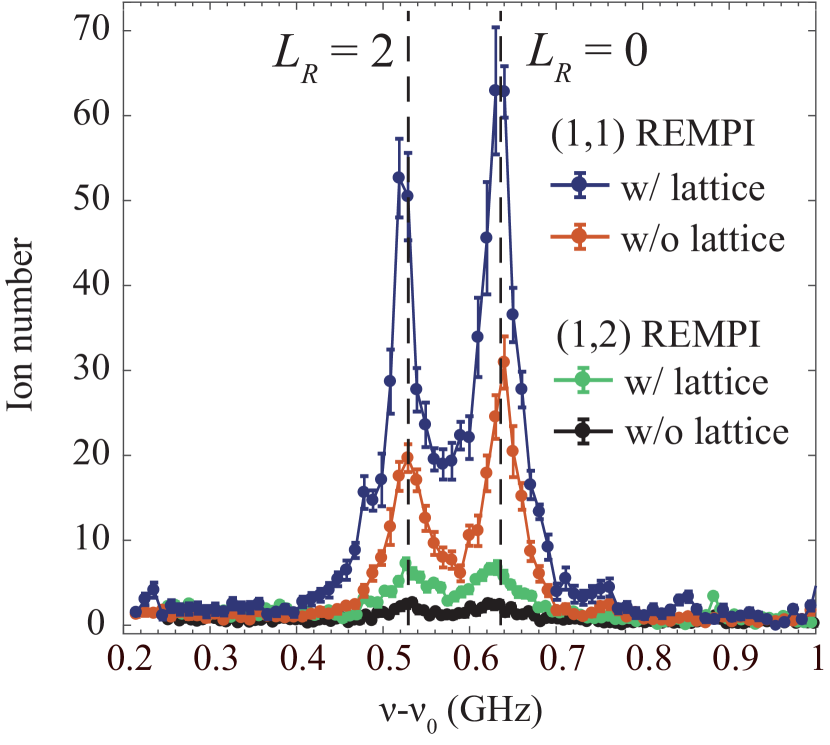
Figure 11: Boost of the molecular detection signal. Shown are measured ion numbers after REMPI of ($\text{\char 118\relax}=-2,L_{R}=0,2$) product molecules as a function of the probe laser frequency $\nu$. $\nu_{0}=281445.045\>\textrm{GHz}$ is the resonance frequency for photoassociation towards the $J^{\prime}=1$ intermediate state. The different colors indicate different measurement configurations as detailed in the legend.

The second improvement step is an enhancement of the REMPI efficiency. In [11, 12] only the first REMPI step in a (1,2) REMPI configuration was resonantly driven. In our new (1,1) scheme [see Fig. 1(a) and Appendix A] both REMPI steps are resonantly driven and the last excitation step is resulting in a molecular state which is probably autoionizing. Switching to the (1,1) REMPI increased the signals by a factor of 10. For comparison, in Fig. 11, the blue and orange data give the signals for (1,1) REMPI with and without lattice, respectively.

In order to optimize REMPI we have also experimentally tested several vibrational levels around $\text{\char 118\relax}^{\prime}=66$ within $A^{1}\Sigma_{u}^{+}$ as intermediate level, but obtained the best results for $\text{\char 118\relax}^{\prime}=66$ in terms of efficiency and suppressing background signals. The level $\text{\char 118\relax}^{\prime}=66$ has essentially a simple rotational ladder structure, as it has unresolved hyperfine splittings of less than $3\>\text{MHz}\times h$ [22, 23].

APPENDIX E Consistency checks for line assignments

In general, we observe each molecular level with $L_{R}>0$ in terms of two transition lines, $L_{R}\rightarrow J^{\prime}=L_{R}\pm 1$. This greatly helps to verify the consistency of the line assignment. As an example, we provide in Fig. 12 the collection of REMPI detection signals for $\text{\char 118\relax}=-4$ molecules with rotational states $L_{R}$ ranging from $L_{R}=0$ to $10$.

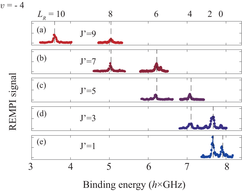
Figure 12: Consistency of assignments of product molecular states to REMPI detection signals. The vertical dashed lines mark the binding energies of the molecules with quantum numbers $\text{\char 118\relax}=-4,L_{R}$ as obtained from coupled channel calculations. The rotational quantum number $L_{R}$ is shown on top of the figure. For each level with $L_{R}>0$ we observe two resonance lines, corresponding to REMPI via the intermediate levels $J^{\prime}=L_{R}\pm 1$. The resonance lines are plotted as a function of the probe laser frequency and are arranged such that the frequency position of each resonance peak is given by $\nu-\nu_{0}-B_{\text{\char 118\relax}^{\prime}=66}\times[J^{\prime}(J^{\prime}+1)-2]$, ideally corresponding to the molecular binding energy. The rotational constant is $B_{\text{\char 118\relax}^{\prime}=66}=443\>\textrm{MHz}$. $\nu_{0}$ is the photoassociation resonance frequency towards $J^{\prime}=1$. In vertical direction the lines are arranged according to $J^{\prime}$. The match in frequency position of the two measured resonance lines and the calculated binding energy for a level indicates consistency of the assignment.

APPENDIX F Three-body model for ⁸⁷Rb atoms

Our three-body calculations for ⁸⁷Rb atoms were performed using the adiabatic hyperspherical representation [25, 18] where the hyperradius $R$ determines the overall size of the system, while all other degrees of freedom are represented by a set of hyperangles $\Omega$. Within this framework, the three-body adiabatic potentials $U_{\alpha}$ and channel functions $\Phi_{\alpha}$ are determined from the solutions of the hyperangular adiabatic equation:

$$\left[\frac{\Lambda^{2}(\Omega)+15/4}{2\mu R^{2}}\hbar^{2}+\sum_{i<j}V(r_{ij})\right]\Phi_{\alpha}(R;\Omega)=U_{\alpha}(R)\Phi_{\alpha}(R;\Omega),$$ (11)

which contains the hyperangular part of the kinetic energy, via the grand-angular momentum operator $\Lambda^{2}$, and the three-body reduced mass $\mu=m/\sqrt{3}$. To calculate the three-body recombination rate we solve the hyperradial Schrödinger equation,

$$\left[-\frac{\hbar^{2}}{2\mu}\frac{d^{2}}{dR^{2}}+U_{\alpha}(R)\right]F_{\alpha}(R)$$

$$~{}~{}~{}~{}~{}~{}+\sum_{\alpha^{\prime}}W_{\alpha\alpha^{\prime}}(R)F_{\alpha^{\prime}}(R)=EF_{\alpha}(R),$$ (12)

where $\alpha$ is an index that labels all necessary quantum numbers to characterize each channel, $E$ is the total energy, and nonadiabatic couplings are given by

$$W_{\alpha\alpha^{\prime}}(R)=-\frac{\hbar^{2}}{2\mu}\left(\langle\Phi_{\alpha}|\frac{d^{2}}{dR^{2}}\Phi_{\alpha^{\prime}}\rangle+2\langle\Phi_{\alpha}|\frac{d}{dR}\Phi_{\alpha^{\prime}}\rangle\frac{d}{dR}\right).$$ (13)

Solving Eq. (12) numerically [18] we determine the $S$-matrix and the recombination rate $L_{3}$ via

$$L_{3}=\sum_{f,i}\frac{96\pi^{2}(2J+1)\hbar}{\mu k_{i}^{4}}|S_{fi}|^{2}=\sum_{f}L_{3}(f),$$ (14)

where $i$ and $f\equiv(\text{\char 118\relax},L_{R})$ represent the initial and final states and $L_{3}(f)$ is the corresponding partial recombination rate for a given final state.

In this present study, the interaction between ⁸⁷Rb atoms is modeled by the same potential used in Ref. [11], and is given by the Lennard-Jones potential,

$$V(r)=-\frac{C_{6}}{r^{6}}\left(1-\frac{\lambda^{6}}{r^{6}}\right),$$ (15)

where $C_{6}=4710.431E_{h}$a${}_{0}^{6}$ is the van der Waals dispersion coefficient from Ref. [26]. We adjust the value of $\lambda$ to have different numbers of diatomic bound states supported by the interaction, while still reproducing the value of the scattering length for ⁸⁷Rb atoms, $a=100.36a_{0}$ [26]. Our calculations were performed using $\lambda\approx 15.5943a_{0}$, producing 15 $s$-wave ($L_{R}=0$) molecular bound states, and a total of 240 bound states including higher partial-wave states, $L_{R}>0$.

Our numerical calculations for three-body recombination through the solutions of Eq. (12) have included up to 300 hyperspherical channels leading to a total rate converged within a few percent. The calculated total recombination rate constant at 0.8$\>\mu$K (including thermal averaging) is $L_{3}\approx 0.91\times 10^{-29}$ cm${}^{6}/$s. We note that there is an unresolved discrepancy between this calculated total three-body recombination rate constant and the corresponding experimental value for Rb in the spin state $f=1,m_{f}=-1$. The experimental value is $L_{3}=(4.3\pm 1.8)\times 10^{-29}\>\text{cm}^{6}\text{s}^{-1}$, [34]. This discrepancy, however, does not affect the analysis of the overall scaling behavior of $L_{3}(\text{\char 118\relax},L_{R})$ with binding energy.

APPENDIX G Interpreting the $1/E_{b}$ scaling law via a perturbative approach

The Alt-Grassberger-Sandhas (AGS) equation is an efficient approach for solving three-particle collision problems [28], and for identical particles it reads [29, 27]

$$U_{0}(E) =\frac{1}{3}G_{0}^{-1}(E)\left[1+P_{+}+P_{-}\right]$$

$$\phantom{=}+\left[P_{+}+P_{-}\right]\mathcal{T}(E)G_{0}(E)U_{0}(E)\,.$$ (16)

Here, the three-body transition operator $U_{0}$ describes the transition process from the initial state of three free, noninteracting atoms to product states of a molecule of the atom pair $(a,b)$ plus a free atom $c$. $E$ denotes the total energy of the three-body system, $G_{0}(E)=(E+i\epsilon-H_{0})^{-1}$ is the free Green’s operator corresponding to the non-interacting three-body Hamiltonian $H_{0}$, and $\epsilon$ is a small quantity to shift the energy away from the real axis. $\mathcal{T}(E)=\int d\mathbf{q}|\mathbf{q}\rangle t(E_{2b})\langle\mathbf{q}|$ represents the generalized two-body transition operator for the interacting pair $(a,b)$ [29, 27]. Here, $t(E_{2b})$ is the pure two-body transition operator at two-body energy $E_{2b}=E-\frac{3q^{2}}{4m}$, $\mathbf{q}$ is the 3-dimensional relative momentum between atom $c$ and the center of mass of the pair $(a,b)$, $m$ is the mass of an atom and $q$ is the absolute value of $\mathbf{q}$. $P_{+}=P_{bc}P_{ab}$ and $P_{-}=P_{ac}P_{ab}$ denote the cyclic and anticyclic permutation operators for the atoms $(a,b,c)$, respectively. The partial three-body recombination rate $L_{3}(\text{\char 118\relax},L_{R})$ towards each specific molecular product $d$ is given by [27]

$$L_{3}(\text{\char 118\relax},L_{R})=\frac{12\pi m}{\hbar}(2\pi\hbar)^{6}q_{d}|\langle\psi_{f}|U_{0}(E)|\psi_{\rm{in}}\rangle|^{2},$$ (17)

where $|\psi_{\rm{in}}\rangle$ and $|\psi_{f}\rangle$ represent the initial and product states, respectively. Here, $q_{d}$ denotes the absolute value of the asymptotic momentum of the molecule which is fixed by the molecule binding energy $E_{b}$ and the total energy $E$ via $\frac{3q_{d}^{2}}{4m}-E_{b}=E$. Iteratively plugging Eq. (G) into its right side, one gets a series expansion $U_{0}(E)=\sum_{n=0}^{\infty}U_{0}^{(n)}(E)$ with $U_{0}^{(n)}(E)=\left\{\left[P_{+}+P_{-}\right]\mathcal{T}(E)G_{0}(E)\right\}^{n}\frac{1}{3}G_{0}^{-1}(E)\left[1+P_{+}+P_{-}\right]$. We assume that the three-body recombination process can be reasonably well described by the leading order contribution for $U_{0}$ [27]. Since $U_{0}^{(0)}(E)|\psi_{\rm{in}}\rangle=\frac{1}{3}\left[1+P_{+}+P_{-}\right](E-H_{0})|\psi_{\rm{in}}\rangle=0$ due to energy conservation, $U_{0}^{(0)}(E)$ has no contribution to the three-body recombination rate according to Eq. (17). Therefore, we approximate $U_{0}(E)$ by $U_{0}^{(1)}(E)$

$$U_{0}(E)\approx\left[P_{+}+P_{-}\right]\mathcal{T}(E)\frac{1}{3}\left[1+P_{+}+P_{-}\right].$$ (18)

Since the three-body recombination rate is usually quite energy independent in the ultracold regime [35], we take the zero energy limit $E\rightarrow 0$ to simplify the derivation. In this limit, the initial free atom state is $|\psi_{\rm{in}}\rangle=|\mathbf{p}=0,\mathbf{q}=0\rangle$, where $\mathbf{p}$ describes the relative momentum between atoms $a$ and $b$. We note that, for identical particles, neither the result of $L_{3}(\text{\char 118\relax},L_{R})$ nor the derivation procedure associated to this quantity should depend on the choice of pair $(a,b)$. Plugging the expression of Eq. (18) into Eq. (17) we obtain

$$L_{3} (\text{\char 118\relax},L_{R})$$

$$\approx \frac{12\pi m}{\hbar}(2\pi\hbar)^{6}q_{d}|\langle\psi_{f}|\left[P_{+}+P_{-}\right]\mathcal{T}(E)\frac{1}{3}\left[1+P_{+}+P_{-}\right]|\psi_{\rm{in}}\rangle|^{2}$$

$$= \frac{12\pi m}{\hbar}(2\pi\hbar)^{6}q_{d}|\langle\psi_{f}|2P_{+}\mathcal{T}(E)|\psi_{\rm{in}}\rangle|^{2},$$ (20)

where we have replaced $P_{+}+P_{-}$ by $2P_{+}$ because the term of $P_{+}$ will contribute equally as the term of $P_{-}$ to $L_{3}(\text{\char 118\relax},L_{R})$, [29, 36]. For similar reasons $[1+P_{+}+P_{-}]/3$ is replaced by 1. In the plane wave basis, $P_{+}$ is given by

$$P_{+}=\int d\mathbf{q}^{\prime}\int d\mathbf{q}^{\prime\prime}|\mathbf{p}^{\prime},\mathbf{q}^{\prime}\rangle\langle\mathbf{p}^{\prime\prime},\mathbf{q}^{\prime\prime}|,$$ (21)

where $\mathbf{p}^{\prime}=\mathbf{q}^{\prime\prime}+\frac{1}{2}\mathbf{q}^{\prime}$ and $\mathbf{p}^{\prime\prime}=-\mathbf{q}^{\prime}-\frac{1}{2}\mathbf{q}^{\prime\prime}$. To derive Eq. (21), we let the single atom momenta be {$\mathbf{k}^{\prime\prime}_{a}=\mathbf{k}_{1}$, $\mathbf{k}^{\prime\prime}_{b}=\mathbf{k}_{2}$, $\mathbf{k}^{\prime\prime}_{c}=\mathbf{k}_{3}$} and by definition we have {$\mathbf{p}^{\prime\prime}=(\mathbf{k}_{2}-\mathbf{k}_{1})/2$, $\mathbf{q}^{\prime\prime}=2\mathbf{k}_{3}/3-\mathbf{k}_{1}/3-\mathbf{k}_{2}/3$}. The permutation operator $P_{+}$ changes the atom indices according to $(a,b,c)\rightarrow(c,a,b)$ and therefore {$\mathbf{k}^{\prime\prime}_{a}=\mathbf{k}_{1}$, $\mathbf{k}^{\prime\prime}_{b}=\mathbf{k}_{2}$, $\mathbf{k}^{\prime\prime}_{c}=\mathbf{k}_{3}$} $\rightarrow$ {$\mathbf{k}^{\prime}_{a}=\mathbf{k}_{2}$, $\mathbf{k}^{\prime}_{b}=\mathbf{k}_{3}$, $\mathbf{k}^{\prime}_{c}=\mathbf{k}_{1}$}, which leads to {$\mathbf{p}^{\prime\prime}=(\mathbf{k}_{2}-\mathbf{k}_{1})/2$, $\mathbf{q}^{\prime\prime}=2\mathbf{k}_{3}/3-\mathbf{k}_{1}/3-\mathbf{k}_{2}/3$} $\rightarrow$ {$\mathbf{p}^{\prime}=(\mathbf{k}_{3}-\mathbf{k}_{2})/2$, $\mathbf{q}^{\prime}=2\mathbf{k}_{1}/3-\mathbf{k}_{2}/3-\mathbf{k}_{3}/3$}, or equivalently, {$\mathbf{p}^{\prime\prime}=-\mathbf{q}^{\prime\prime}/2-\mathbf{q}^{\prime}$, $\mathbf{q}^{\prime\prime}$} $\rightarrow$ {$\mathbf{p}^{\prime}=\mathbf{q}^{\prime}/2+\mathbf{q}^{\prime\prime}$, $\mathbf{q}^{\prime}$}. It is then straightforward that $P_{+}=\int d\mathbf{q}^{\prime}\int d\mathbf{q}^{\prime\prime}|\mathbf{p}^{\prime}=\mathbf{q}^{\prime}/2+\mathbf{q}^{\prime\prime},\mathbf{q}^{\prime}\rangle\langle\mathbf{p}^{\prime\prime}=-\mathbf{q}^{\prime\prime}/2-\mathbf{q}^{\prime},\mathbf{q}^{\prime\prime}|$. Using the previous expressions for $P_{+}$ and $\mathcal{T}(E)$, and $|\psi_{\rm{in}}\rangle=|\mathbf{p}=\mathbf{0},\mathbf{q=\mathbf{0}}\rangle$, we find

$$\langle\psi_{f}|P_{+}\mathcal{T}(E)|\psi_{\rm{in}}\rangle$$

$$= \langle\psi_{f}|\int d\mathbf{q}^{\prime}\int d\mathbf{q}^{\prime\prime}|\mathbf{p}^{\prime},\mathbf{q}^{\prime}\rangle\langle\mathbf{p}^{\prime\prime},\mathbf{q}^{\prime\prime}|\int d\mathbf{\tilde{q}}|\mathbf{\tilde{q}}\rangle t(E-\frac{3{\tilde{q}}^{2}}{4m})\langle\mathbf{\tilde{q}}|\psi_{\rm{in}}\rangle$$

$$= \langle\psi_{f}|\int d\mathbf{q}^{\prime}\int d\mathbf{q}^{\prime\prime}|\mathbf{p}^{\prime},\mathbf{q}^{\prime}\rangle\langle\mathbf{q}^{\prime\prime}|0\rangle\langle\mathbf{p}^{\prime\prime}|t(0)|\mathbf{p}=0\rangle$$

$$= \int d\mathbf{q}^{\prime}\langle\psi_{f}|\mathbf{p}^{\prime},\mathbf{q}^{\prime}\rangle\langle\mathbf{p}^{\prime\prime}|t(0)|\mathbf{p}=0\rangle,$$

where we have used $\langle\mathbf{q}^{\prime}|\mathbf{\tilde{q}}\rangle=\delta(\mathbf{q}^{\prime}-\mathbf{\tilde{q}})$, and in the last line we have $\mathbf{p}^{\prime}=\frac{1}{2}\mathbf{q}^{\prime}$ and $\mathbf{p}^{\prime\prime}=-\mathbf{q}^{\prime}$. We now switch from the plane wave basis to a partial wave basis by using

$$|\mathbf{p}\rangle=|p\rangle\sum_{l,m}Y_{l,m}^{*}(\mathbf{e_{p}})|l,m\rangle,$$ (23)

where $p=|\mathbf{p}|$, $\mathbf{e_{p}}=\mathbf{p}/p$ and the normalization of $|p\rangle$ is given by $\langle p^{\prime}|p\rangle=\frac{\delta(p-p^{\prime})}{p^{2}}$. The expression $\langle\mathbf{p}^{\prime\prime}|t(0)|\mathbf{p}=0\rangle$ in the last line of Eq. (G) can be expressed as

$$\langle-\mathbf{q^{\prime}}|t(0)|\mathbf{p}=0\rangle = \frac{1}{4\pi}\langle q^{\prime}|t^{s}(0)|p=0\rangle,$$ (24)

where $t^{s}$ is the $s$-wave component of the two-body transition operator $t$. Here we have used that according to the Wigner threshold law at low collision energies only $s$-wave collisions can contribute. Furthermore, we assume that the interaction between two atoms conserves angular momentum.

Next, we consider the expression $\langle\psi_{f}|\mathbf{p}^{\prime}=\frac{1}{2}\mathbf{q}^{\prime},\mathbf{q}^{\prime}\rangle$. For $|\psi_{f}\rangle$ we make the Ansatz $|\psi_{f}\rangle=|\phi_{d}\rangle|q_{d},\hat{l},\hat{m}\rangle$. Here, $|\phi_{d}\rangle=|L_{R},m_{L_{R}}\rangle\,\int dp\,p^{2}\phi_{d}(p)|p\rangle$ is the internal wave function of the molecule with rotational angular momentum quantum numbers $L_{R},m_{L_{R}}$. $\phi_{d}(p)$ is normalized via $\int|\phi_{d}(p)|^{2}p^{2}dp=1$. The state $|q_{d},\hat{l},\hat{m}\rangle\equiv|q_{d}\rangle|\hat{l},\hat{m}\rangle$ describes the relative motion between molecule and atom. It corresponds to a partial wave with rotational quantum numbers $\hat{l},\hat{m}$. Next, we calculate that

$$\langle\phi_{d}|\frac{1}{2}\mathbf{q^{\prime}}\rangle = \phi_{d}^{*}\left(\frac{1}{2}q^{\prime}\right)\,\,Y^{*}_{L_{R},m_{L_{R}}}(\mathbf{e_{q^{\prime}}})\,,$$ (25)

$$\langle q_{d},\hat{l},\hat{m}|\mathbf{q^{\prime}}\rangle = \frac{\delta(q_{d}-q^{\prime})}{q^{2}}\,\,Y^{*}_{\hat{l},\hat{m}}(\mathbf{e_{q^{\prime}}})\,.$$ (26)

Plugging the results of Eqs. (24) to (26) into Eq. (G) and carrying out the integration over $\mathbf{q^{\prime}}$ we obtain

$$\langle\psi_{f}|P_{+}\mathcal{T}(E)|\psi_{\rm{in}}\rangle$$

$$= \frac{(-1)^{m}}{4\pi}\phi^{*}_{d}(\frac{1}{2}q_{d})\,\langle q_{d}|t^{s}(0)|p=0\rangle\,\delta_{L_{R},\hat{l}}\delta_{m_{L_{R}},-\hat{m}},$$

where we have used $\int d\Omega_{q}Y^{*}_{lm}(\mathbf{e_{q}})Y^{*}_{l^{\prime}m^{\prime}}(\mathbf{e_{q}})=(-1)^{m}\delta_{l,l^{\prime}}\delta_{m,-m^{\prime}}$. We then define

$$t_{\rm{h}}(q_{d})=\langle q_{d}|t^{s}(0)|p=0\rangle$$ (28)

and use Eq. (G) to rewrite Eq. (G) as

$$L_{3}(\text{\char 118\relax},L_{R})\approx\frac{12\pi m}{\hbar}(2\pi\hbar)^{6}q_{d}(2L_{R}+1)|\frac{1}{2\pi}\phi_{d}\left(\frac{1}{2}q_{d}\right)t_{\rm{h}}(q_{d})|^{2}.$$ (29)

Here, we have summed over the $2L_{R}+1$ equal contributions corresponding to the available $m_{d}$-channels for a given $L_{R}$ quantum number. $t_{\rm{h}}(q_{d})$ has momentum $p=0$ fixed on the energy shell $p^{2}/m=E_{2b}=0$, and is commonly referred to as half-shell $t$-matrix in nuclear physics [37, 38].

In order to analyze the scaling of $L_{3}(\text{\char 118\relax},L_{R})$ with the molecular binding energy $E_{b}$, we use the relation $\frac{3q_{d}^{2}}{4m}-E_{b}=0$ and ignore all coefficients independent on $q_{d}$ in Eq. (29) to obtain

$$L_{3}(\text{\char 118\relax},L_{R})\propto(E_{b})^{1/2}|\phi_{d}(\sqrt{mE_{b}/3})|^{2}|t_{\rm{h}}(2\sqrt{mE_{b}/3})|^{2}.$$ (30)

In Fig. 13(a) we show $t_{\rm{h}}(p)$. It oscillates but the amplitude varies only slowly with the two-body momentum $p$. Of course, this only holds until the bottom of the interaction potential (corresponding to the most deeply-bound states) is reached, as the bottom leads to a momentum cut-off. Figure 13(b) shows $\phi_{d}(p)$ which is discussed in the main text.

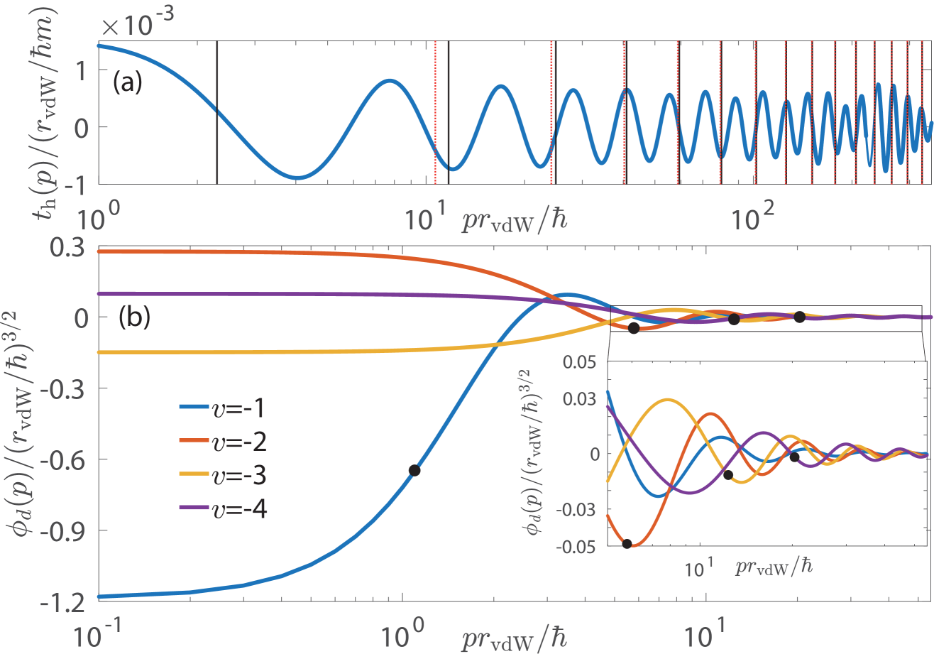
Figure 13: (a) Two-body half-shell $t$-matrix $t_{\rm{h}}$ as a function of the relative two-body momentum $p$. The vertical lines indicate the momentum values $2\sqrt{mE_{b}/3}$ corresponding to $s$-wave (black solid) and $d$-wave (red dotted) molecules where $t_{\rm{h}}$ needs to be evaluated. (b) Momentum space wave functions of the four most shallow $s$-wave molecules. The dots indicate the momentum values $\sqrt{mE_{b}/3}$ where $\phi_{d}$ needs to be evaluated. These results are obtained from a Lennard-Jones potential with 15 $s$-wave molecular states and a scattering length $a=1.21$ $r_{\rm{vdW}}$. Here, $r_{\rm{vdW}}=\frac{1}{2}(mC_{6}/\hbar^{2})^{1/4}$ is the characteristic length scale of the van der Waals interaction. Given $r_{\rm{vdW}}=82.64$ a₀ for ⁸⁷Rb, this scattering length corresponds to $a=100.36$ a₀.

References

- Yang [2007] X. Yang, State-to-state dynamics of elementary bimolecular reactions, Annu. Rev. Phys. Chemi. 58, 433 (2007).
- Pan et al. [2017] H. Pan, K. Liu, A. Caracciolo, and P. Casavecchia, Crossed beam polyatomic reaction dynamics: recent advances and new insights, Chem. Soc. Rev. 46, 7517 (2017).
- Jankunas and Osterwalder [2015] J. Jankunas and A. Osterwalder, Cold and controlled molecular beams: Production and applications, Annu. Rev. Phys. Chem. 66, 241 (2015).
- van de Meerakker et al. [2012] S. Y. T. van de Meerakker, H. L. Bethlem, V. C., and G. Meijer, Manipulation and control of molecular beams, Chem. Rev. 112, 4828 (2012).
- Liu et al. [2020] Y. Liu, D. D. Grimes, M.-G. Hu, and K.-K. Ni, Probing ultracold chemistry using ion spectrometry, Phys. Chem. Chem. Phys. 22, 4861 (2020).
- Härter et al. [2013a] A. Härter, A. Krükow, M. Deiß, B. Drews, E. Tiemann, and J. Hecker Denschlag, Population distribution of product states following three-body recombination in an ultracold atomic gas, Nat. Phys. 9, 512 (2013a).
- Paliwal et al. [2021] P. Paliwal, N. Deb, D. M. Reich, A. vam der Avoird, C. P. Koch, and E. Narevicius, Determining the nature of quantum resonances by probing elastic and reactive scattering in cold collisions, Nat. Chem. 13, 94 (2021).
- de Jongh et al. [2020] T. de Jongh, M. Besemer, Q. Shuai, T. Karman, A. van der Avoird, G. C. Groenenboom, and S. Y. T. van de Meerakker, Imaging the onset of the resonance regime in low-energy NO-He collisions, Science 368, 626 (2020).
- Beyer and Merkt [2018] M. Beyer and F. Merkt, Half-collision approach to cold chemistry: Shape resonances, elastic scattering, and radiative association in the and collision systems, Phys. Rev. X 8, 031085 (2018).
- Haze et al. [2022] S. Haze, J. P. D’Incao, D. Dorer, M. Deiß, E. Tiemann, P. S. Julienne, and J. H. Denschlag, Spin-conservation propensity rule for three-body recombination of ultracold Rb atoms, Phys. Rev. Lett. 128, 133401 (2022).
- Wolf et al. [2017] J. Wolf, M. Deiß, A. Krükow, E. Tiemann, B. P. Ruzic, Y. Wang, J. P. D’Incao, P. S. Julienne, and J. Hecker Denschlag, State-to-state chemistry for three-body recombination in an ultracold rubidium gas, Science 358, 921 (2017).
- Wolf et al. [2019] J. Wolf, M. Deiß, and J. Hecker Denschlag, Hyperfine magnetic substate resolved state-to-state chemistry, Phys. Rev. Lett. 123, 253401 (2019).
- Hu et al. [2021] M.-G. Hu, Y. Liu, M. A. Nichols, L. Zhu, G. Quéméner, O. Dulieu, and K.-K. Ni, Nuclear spin conservation enables state-to-state control of ultracold molecular reactions, Nat. Chem. 13, 435 (2021).
- Liu et al. [2021] Y. Liu, M.-G. Hu, M. A. Nichols, D. Yang, D. Xie, H. Guo, and K.-K. Ni, Precision test of statistical dynamics with state-to-state ultracold chemistry, Nature 593, 379 (2021).
- Weber et al. [2003] T. Weber, J. Herbig, M. Mark, H.-C. Nägerl, and R. Grimm, Three-body recombination at large scattering lengths in an ultracold atomic gas, Phys. Rev. Lett. 91, 123201 (2003).
- Jochim et al. [2003] S. Jochim, M. Bartenstein, A. Altmeyer, G. Hendl, C. Chin, J. Hecker Denschlag, and R. Grimm, Pure gas of optically trapped molecules created from fermionic atoms, Phys. Rev. Lett. 91, 240402 (2003).
- Wang et al. [2022] B.-B. Wang, M. Zhang, and Y.-C. Han, Ultracold state-to-state chemsitry for three-body recombination in realistic 3He2-alkaline-earth-metal systems, J. Chem. Phys. 157, 014305 (2022).
- Wang et al. [2011] J. Wang, J. P. D’Incao, and C. H. Greene, Numerical study of three-body recombination for systems with many bound states, Phys. Rev. A 84, 052721 (2011).
- Pérez-Ríos et al. [2014] J. Pérez-Ríos, S. Ragole, J. Wang, and C. H. Greene, Comparison of classical and quantal calculations of helium three-body recombination, J. Chem. Phys. 140, 044307 (2014).
- Yuen and Kokoouline [2020] C. H. Yuen and V. Kokoouline, Jahn-Teller effect in three-body recombination of hydrogen atoms, Phys. Rev. A 101, 042709 (2020).
- Nesbitt [2012] D. J. Nesbitt, Toward state-to-state dynamics in ultracold collisions: Lessons from high-resolution spectroscopy of weakly bound molecular complexes, Chem. Rev. 112, 5062 (2012).
- Deiß et al. [2015] M. Deiß, B. Drews, J. Hecker Denschlag, and E. Tiemann, Mixing of and observed in the hyperfine and Zeeman structure of ultracold Rb2 molecules, New J. Phys. 17, 083032 (2015).
- Drozdova et al. [2013] A. N. Drozdova, A. V. Stolyarov, M. Tamanis, R. Ferber, P. Crozet, and A. J. Ross, Fourier transform spectroscopy and extended deperturbation treatment of the spin-orbit-coupled and states of the Rb2 molecule, Phys. Rev. A 88, 022504 (2013).
- [24] Up to binding energies of our measurements confirm the previously found propensity rules for the conservation of the angular momentum quantum numbers in three-body recombination [11, 10, 12]. Here, , and are the quantum numbers for the initial total angular momenta and of the two atoms that combine to form the molecule, and with corresponding magnetic quantum number .
- D’Incao [2018] J. P. D’Incao, Few-body physics in resonantly interacting ultracold quantum gases, J. Phys. B: At. Mol. Opt. Phys. 51, 043001 (2018).
- Strauss et al. [2010] C. Strauss, T. Takekoshi, F. Lang, K. Winkler, R. Grimm, J. Hecker Denschlag, and E. Tiemann, Hyperfine, rotational, and vibrational structure of the state of 2, Phys. Rev. A 82, 052514 (2010).
- Li et al. [2022] J.-L. Li, T. Secker, P. M. A. Mestrom, and S. J. J. M. F. Kokkelmans, Strong spin-exchange recombination of three weakly interacting atoms, Phys. Rev. Research 4, 023103 (2022).
- Alt et al. [1967] E. Alt, P. Grassberger, and W. Sandhas, Reduction of the three-particle collision problem to multi-channel two-particle Lippmann-Schwinger equations, Nuclear Physics B 2, 167 (1967).
- Secker et al. [2021] T. Secker, J.-L. Li, P. M. A. Mestrom, and S. J. J. M. F. Kokkelmans, Multichannel nature of three-body recombination for ultracold , Phys. Rev. A 103, 022825 (2021).
- [30] Technically, depends on . This dependence, however, is so weak that its effect on the scaling is negligible.
- Chin et al. [2010] C. Chin, R. Grimm, P. Julienne, and E. Tiesinga, Feshbach resonances in ultracold gases, Rev. Mod. Phys. 82, 1225 (2010).
- Härter et al. [2013b] A. Härter, A. Krükow, A. Brunner, and J. Hecker Denschlag, Minimization of ion micromotion using ultracold atomic probes, Appl. Phys. Lett. 102, 221115 (2013b).
- Mohammadi et al. [2021] A. Mohammadi, A. Krükow, A. Mahdian, M. Deiß, J. Pérez-Ríos, H. da Silva, M. Raoult, O. Dulieu, and J. Hecker Denschlag, Life and death of a cold BaRb+ molecule inside an ultracold cloud of Rb atoms, Phys. Rev. Research 3, 013196 (2021).
- Burt et al. [1997] E. A. Burt, R. W. Ghrist, C. J. Myatt, M. J. Holland, E. A. Cornell, and C. E. Wieman, Coherence, correlations, and collisions: What one learns about Bose-Einstein condensates from their decay, Phys. Rev. Lett. 79, 337 (1997).
- Suno et al. [2002] H. Suno, B. D. Esry, C. H. Greene, and J. P. Burke, Three-body recombination of cold helium atoms, Phys. Rev. A 65, 042725 (2002).
- Glöckle [1983] W. Glöckle, The quantum mechanical few-body problem, Texts and monographs in physics (Springer, Berlin, 1983).
- Ernst et al. [1973] D. J. Ernst, C. M. Shakin, and R. M. Thaler, Separable representations of two-body interactions, Phys. Rev. C 8, 46 (1973).
- Hlophe et al. [2013] L. Hlophe, C. Elster, R. C. Johnson, N. J. Upadhyay, F. M. Nunes, G. Arbanas, V. Eremenko, J. E. Escher, and I. J. Thompson (TORUS Collaboration), Separable representation of phenomenological optical potentials of woods-saxon type, Phys. Rev. C 88, 064608 (2013).