Lower Bounds for the Convergence of Tensor Power Iteration on Random Overcomplete Models

Abstract

Tensor decomposition serves as a powerful primitive in statistics and machine learning. In this paper, we focus on using power iteration to decompose an overcomplete random tensor. Past work studying the properties of tensor power iteration either requires a non-trivial data-independent initialization, or is restricted to the undercomplete regime. Moreover, several papers implicitly suggest that logarithmically many iterations (in terms of the input dimension) are sufficient for the power method to recover one of the tensor components.

In this paper, we analyze the dynamics of tensor power iteration from random initialization in the overcomplete regime. Surprisingly, we show that polynomially many steps are necessary for convergence of tensor power iteration to any of the true component, which refutes the previous conjecture. On the other hand, our numerical experiments suggest that tensor power iteration successfully recovers tensor components for a broad range of parameters, despite that it takes at least polynomially many steps to converge. To further complement our empirical evidence, we prove that a popular objective function for tensor decomposition is strictly increasing along the power iteration path.

Our proof is based on the Gaussian conditioning technique, which has been applied to analyze the approximate message passing (AMP) algorithm. The major ingredient of our argument is a conditioning lemma that allows us to generalize AMP-type analysis to non-proportional limit and polynomially many iterations of the power method.

1 Introduction

Tensors of order $m$ are multidimensional arrays with $m$ indices, with $m=1$ corresponding to vectors and $m=2$ corresponding to matrices. The notion of rank naturally generalizes from matrices to tensors: An $m$-th order tensor $\mathrm{\bf T}\in(\mathbb{R}^{d})^{\otimes m}$ is said to have rank-1 if it can be written as

$$\mathrm{\bf T}=v_{1}\otimes\cdots\otimes v_{m}\Longleftrightarrow\mathrm{\bf T}(i_{1},\cdots,i_{m})=v_{1}(i_{1})\cdots v_{m}(i_{m}),$$

where $v_{1},\cdots,v_{m}\in\mathbb{R}^{d}$. Past results imply that any tensor can be expressed as the sum of rank-1 tensors [Kie00, CC70]. Namely, given $\mathrm{\bf T}\in(\mathbb{R}^{d})^{\otimes m}$ we can find vectors $\{v_{i}^{(j)}\}_{i\in[m],\ j\in[k]}$ such that

$$\mathrm{\bf T}=\sum_{j=1}^{k}v_{1}^{(j)}\otimes\cdots\otimes v_{m}^{(j)}.$$

The above decomposition is referred to as tensor decomposition, and the (CP) rank of a tensor is defined as the minimum number of rank-1 tensors required in such decomposition. Unlike matrix decomposition, tensor decomposition with $m\geq 3$ is in many cases unique [Kru77]. This is often true even in the overcomplete case, where the rank of the tensor is much larger than its ambient dimension. The uniqueness of tensor decomposition makes its application suitable in many practical settings, which we discuss below.

Tensor decomposition serves as a powerful primitive in statistics and machine learning, especially for algorithms that leverage the method of moments [Pea94] to learn model parameters. Applications of tensor decomposition include dictionary learning [BKS15, MSS16, SS17], Gaussian mixture models [AGH⁺14, GHK15, HK13], independent component analysis [DLCC07, CJ10], and learning two-layer neural networks [NPOV15, MM19]. Despite the fact that tensor decomposition is NP-hard in the worst case [HL13], researchers have designed polynomial-time algorithms that successfully approximate the tensor components under natural distributional assumptions. Exemplary algorithms of this kind include the classical Jennrich’s algorithm [H⁺70, DLDMV96], iterative methods [ZG01, AGH⁺14, AGJ14, AGJ15, AGJ17, KP19, KKMP21], sum-of-squares (SOS) algorithms [HSS15, BKS15, GM15, MSS16] and their spectral analogues [HSSS16, SS17, HSS19, DdL⁺22].

SOS algorithms and their spectral counterparts provably achieve strong guarantees of recovering tensor components, and can be implemented in polynomial time. However, they are often computationally prohibitive on large-scale problems due to the high-degree polynomial running time. Therefore, in practice it is often more preferable to resort to simple iterative algorithms [CMW20, MW22b], such as gradient descent and its variants. These algorithms are computationally efficient in terms of both runtime and memory, and are typically easy to implement. In the case of tensors, popular iterative algorithms include tensor power iteration [AGJ17], gradient descent on non-convex losses [GM17], and alternating minimization [AGJ14].

We focus in this paper on the tensor power iteration method, which can be regarded as a generalization of matrix power iteration. This method can also be viewed as gradient ascent on a polynomial objective function with infinite step size (see Eq. (2) for a formal definition). However, unlike the matrix case where the convergence properties are well understood theoretically, in the tensor case the dynamics of power iteration still remains mysterious due to non-convexity of the corresponding optimization problem. To unveil the mystery behind tensor power iteration, the present work proposes to study its asymptotic behavior on decomposing a random fourth order symmetric tensor

$$\mathrm{\bf T}=\sum_{i=1}^{k}a_{i}\otimes a_{i}\otimes a_{i}\otimes a_{i},\ a_{i}\in\mathbb{R}^{d},\ \forall i\in[k]$$

in the overcomplete regime $k\gg d$, where we assume $a_{i}\overset{\scriptsize\mathrm{i.i.d.}}{\sim}{\sf N}(0,I_{d}/d)$. We note that this is a well-studied model in the literature, while its properties are not yet fully understood. Given the entries of $\mathrm{\bf T}$, our goal is to recover one or all of the tensor components $\{a_{i}\}_{i\leq k}$, up to potential sign flips.

We denote by $A\in\mathbb{R}^{k\times d}$ the matrix whose $i$-th row is $a_{i}^{\sf T}$. Initialized at $x_{0}\in\mathbb{S}^{d-1}(\sqrt{d})$ that is independent of the tensor components $\{a_{i}\}_{i\leq k}$, tensor power iteration is defined recursively as follows:

$$x_{t}=\frac{\sqrt{d}\,\mathrm{\bf T}(I,x_{t-1},x_{t-1},x_{t-1})}{\|\mathrm{\bf T}(I,x_{t-1},x_{t-1},x_{t-1})\|_{2}},\ t\geq 1,$$ (1)

where

$$\mathrm{\bf T}(I,x,x,x):=\sum_{i,j,l\in[d]}x(i)x(j)x(l)\mathrm{\bf T}(:,i,j,l).$$

For $x\in\mathbb{S}^{d-1}(\sqrt{d})$, we introduce the following polynomial objective function:

$$\mathcal{S}(x)=\sum_{i,j,k,l\in[d]}\mathrm{\bf T}(i,j,k,l)x(i)x(j)x(k)x(l)=\sum_{i=1}^{k}\langle a_{i},x\rangle^{4}=\left\|{Ax}\right\|_{4}^{4}.$$ (2)

Notice that Eq. (1) can be reformulated as $x_{t}=\sqrt{d}\cdot\nabla\mathcal{S}(x_{t-1})/\left\|{\nabla\mathcal{S}(x_{t-1})}\right\|_{2}$, i.e., tensor power iteration can be regarded as gradient ascent on $\mathcal{S}$ with infinite learning rate.

In the undercomplete regime where $k\leq d$, if the components $\{a_{i}\}_{i\leq k}$ are orthogonal to each other, then $\mathcal{S}$ has only $2k$ local maximizers that are close to $\{\pm\sqrt{d}a_{i}\}_{i\leq k}$. In this case, tensor power iteration provably converges to one of the $\pm\sqrt{d}a_{i}$’s [AGH⁺14]. Indeed, tensors with linearly independent components can be orthogonalized, thus suggesting the existence of efficient algorithms in the undercomplete regime.

Things become far more challenging in the overcomplete regime where $k$ is much greater than $d$. When $k\ll d^{2}$, it is known that any global maximizer of $\mathcal{S}$ must be close to one of the $\pm\sqrt{d}a_{i}$’s. However, algebraic geometry techniques show that $\mathcal{S}$ has exponentially many other critical points [CS13]. Further, if $k\gg d^{2}$, then $\mathcal{S}(x)$ concentrates tightly around its expectation, uniformly for all $x\in\mathbb{S}^{d-1}(\sqrt{d})$, thus making it hard to identify the tensor components from the information encoded in $\mathcal{S}$. As far as we know, there is no polynomial-time algorithm known for tensor decomposition in this regime.

We thus focus on the regime $d\ll k\ll d^{2}$, where SOS-based algorithms are proven to succeed [GM15, MSS16, HSSS16, DdL⁺22], and numerical experiments indicate that the performance of randomly initialized power iteration matches that of SOS-based methods (see Fig. 1 for details). However, from a theoretical standpoint, the dynamics of tensor power iteration in the overcomplete regime still remain elusive. A reasonable first step towards solving this puzzle would be to understand how many iterations are necessary for power method to find one of the true components.

1.1 Main results

We hereby give a partial answer to the above question. In particular, we establish several new results on the behavior of tensor power iteration in the overcomplete regime. Our first theorem states that randomly initialized tensor power iteration requires at least polynomially many steps to converge to a true component:

Theorem 1.1 (Slow convergence from random start, informal, see 3.1).

Assume that $k$, $d$ are large enough, and that $k\asymp d^{c}$ for some $c\in(3/2,2)$. Then, there exists some $\eta>0$ that only depends on $c$, such that with high probability the following happens: Tensor power iteration from random initialization fails to identify any true component of $\mathrm{\bf T}$ within $d^{\eta}$ steps.

Related work. Let us pause here to make some comparisons between our result and prior work on the same model: The seminal paper [AGJ15] shows that tensor power iteration with an SVD-based initialization converges in $O(\log d)$ steps for $k=O(d)$. In [AGJ17], the authors prove that tensor power method successfully recovers one of the $a_{i}$’s in $O(\log\log d)$ iterations, given that its initialization has non-trivial correlations with the true components. As a comparison, our Theorem 1.1 shows that the $O(\log d)$ bound on the number of iterations does not hold for randomly-initialized power iteration, and establishes that polynomially many steps are necessary for convergence in the overcomplete regime. To the best of our knowledge, this is the first result that provides a lower bound on the computational complexity of tensor power iteration. From a more fundamental point of view, we also show that tensor power iterates are “trapped” in a small neighborhood around its initialization for polynomially many steps.

Although the power method fails to converge in logarithmic many steps as conjectured, we still believe that it will correctly learn one of the tensor components when $k\ll d^{2}$ within polynomial time. We present numerical evidence as Fig. 1 in Section 4 to support our claim. Establishing a rigorous positive result for tensor power iteration in this regime is challenging, and we leave it as an interesting open question for future work. As an alternative, we present here a weaker result suggesting the correctness of tensor power iteration.

Theorem 1.2 (Increasing objective function, informal, see 3.2).

For $d^{3/2}\ll k\ll d^{2}$, starting from random initialization, with high probability the objective function $\mathcal{S}$ is strictly increasing along the power iteration path up to finitely many steps.

According to [GM17], the tensor components are the only local maximizers of $\mathcal{S}$ on a superlevel set that is slightly better than random initialization. Their result, together with 1.2 suggest that, in order to prove convergence of tensor power iteration, it suffices to show that the objective function $\mathcal{S}$ eventually surpasses a small threshold determined in [GM17].

Proof technique. Our proof is based on the Gaussian conditioning technique, and is similar to the analysis of the Approximate Message Passing (AMP) algorithm [BM11]. The majority of prior AMP theory can only accommodate a constant number of iterations (i.e., the number of iterations does not grow with the input size) and proportional asymptotics (in our case, this corresponds to assuming $k/d\to\delta\in(0,\infty)$). [RV18] moves beyond the constant regime and extends Gaussian conditioning analysis to $O(\log d/\log\log d)$ many steps. However, their results fall short of validity when targeting for polynomially many iterations, which is essential in our context. More recently, [LW22] develops a non-asymptotic framework that enables the analysis of AMP up to $O(n/\mbox{poly}\log n)$ many iterations, while they focus exclusively on symmetric spiked model and require nontrivial initialization.

The technical innovation in this paper is that we successfully apply the Gaussian conditioning scheme to analyze the tensor power iteration up to polynomially many steps. Indeed, our conditioning lemma (Lemma 2.1) gives an exact non-asymptotic characterization of the power iterates, thus allowing for precisely tracking the values of the objective function along the iteration path. It is noteworthy that the same argument can be used to prove that polynomially many power iterates are necessary for general even-order tensors (see Remark 3.1). To the best of our knowledge, this is the first result that generalizes AMP-type analysis to non-proportional asymptotics and polynomially many iterations. From a technical perspective, we believe our results will help to push forward the development of AMP theory and enrich the toolbox for theoretical analysis of general iterative algorithms.

Organization. The rest of this paper is organized as follows. Section 2 introduces some preliminaries regarding power iteration and Gaussian conditioning technique. In Section 3 we state formally our main theorems and sketch their proofs, with all technical details deferred to the appendices. Section 4 provides some useful numerical experiments that support our theoretical results. We provide in Section 5 several concluding remarks and discuss possible future directions.

2 Preliminaries

2.1 Notation

For $x\in\mathbb{R}^{d}$ and $S\in\mathbb{R}^{d\times k}$, we denote by $\Pi_{S}(x)$ the projection of $x$ onto the column space of $S$, and let $\Pi_{S}^{\perp}(x)=x-\Pi_{S}(x)$. For two vectors $u$ and $v$ of the same dimension, we use $\langle u,v\rangle$ to represent their inner product, and denote by $\left\|{u}\right\|_{p}$ the $\ell^{p}$-norm of $u$ for $p\geq 1$. We use the notation $\odot$ to represent the Hadamard product of vectors and matrices. Furthermore, for $x\in\mathbb{R}^{d}$ we define $x^{k}={x\odot x\cdots\odot x}$, the Hadamard product of $k$ copies of $x$. For a matrix $X$, we denote by $X^{\dagger}$ the pseudoinverse of $X$.

We denote by $\mathbb{S}^{d-1}(r)$ the sphere in $\mathbb{R}^{d}$ centered at the origin with radius $r$. For random variables $X,Y$, we write $X\perp Y$ if $X$ is independent of $Y$. For a collection of random variables $\{X_{i}\}_{i\in I}$, we use $\sigma(\{X_{i}\}_{i\in I})$ to represent the $\sigma$-algebra generated by these random variables.

For $n\in\mathbb{N}_{+}$, we define the set $[n]:=\{1,2,\cdots,n\}$. For two sequences of positive numbers $\{a_{n}\}_{n\in\mathbb{N}_{+}}$, $\{b_{n}\}_{n\in\mathbb{N}_{+}}$, we say $a_{n}\ll b_{n}$ if $a_{n}/b_{n}\to 0$ as $n\to\infty$. For $\{c_{n}\}_{n\in\mathbb{N}_{+}}\subseteq\mathbb{R}$, we say $c_{n}=o_{n}(1)$ if $c_{n}\to 0$ as $n\to\infty$. For a sequence of events $\{E_{n}\}_{n\in\mathbb{N}_{+}}$, we say that $E_{n}$ happens with high probability if $\mathbb{P}(E_{n})=1-o_{n}(1)$.

We reserve $O_{P}$ and $o_{P}$ as the standard big-$O$/small-$o$ in probability notations: For a set of random variables $\{X_{n}\}_{n\geq 1}$ and a sequence of positive numbers $\{a_{n}\}_{n\geq 1}$, we say $X_{n}=o_{P}(a_{n})$ if and only if for all $\delta>0$, $\lim_{n\to\infty}\mathbb{P}(|X_{n}/a_{n}|>\delta)\to 0$. Similarly, we say $X_{n}=O_{P}(a_{n})$ if and only if for all $\delta>0$, there exists $M,N\in\mathbb{R}_{+}$, such that $\mathbb{P}(|X_{n}/a_{n}|>M)<\delta$ for all $n>N$.

Throughout the proof, with a slight abuse of notation, we use capital letter $C$ to represent various numerical constants, the values of which might not necessarily be the same in each occurrence.

2.2 Tensor power iteration

Using the rank-one decomposition of $\mathrm{\bf T}$, we can reformulate the tensor power iteration stated in Eq. 1 as follows:

$$x_{t}=\sqrt{d}\cdot\frac{\sum_{i=1}^{k}\langle a_{i},x_{t-1}\rangle^{3}a_{i}}{\left\|{\sum_{i=1}^{k}\langle a_{i},x_{t-1}\rangle^{3}a_{i}}\right\|_{2}},\qquad t\geq 1.$$

For notational convenience, we recast $x_{t}$ as $\widetilde{x}_{t}$, and redefine

$$x_{t}:=\sum_{i=1}^{k}\langle a_{i},\widetilde{x}_{t-1}\rangle^{3}a_{i}=A^{\sf T}(A\widetilde{x}_{t-1})^{3},$$

where we recall that $A\in\mathbb{R}^{k\times d}$ is the matrix whose $i$-th row is $a_{i}^{\sf T}$. In other words, $x_{t}$ is the gradient of $\mathcal{S}(x)=\left\|{Ax}\right\|_{4}^{4}$ at $\widetilde{x}_{t-1}$, and $\widetilde{x}_{t}$ is the projection of $x_{t}$ onto $\mathbb{S}^{d-1}(\sqrt{d})$:

$$x_{t}=A^{\sf T}(A\widetilde{x}_{t-1})^{3},\ \widetilde{x}_{t}=\sqrt{d}\cdot\frac{x_{t}}{\left\|{x_{t}}\right\|_{2}}.$$

We introduce some useful intermediate variables: $y_{t}=A\widetilde{x}_{t-1}$, $f_{t}=y_{t}^{3}$. Using these intermediate variables, tensor power iteration can be decomposed into the following steps:

$$\begin{split}&y_{t}=A\widetilde{x}_{t-1},\qquad f_{t}=y_{t}^{3},\\ &x_{t}=A^{{\sf T}}f_{t},\qquad\widetilde{x}_{t}=\sqrt{d}\cdot\frac{x_{t}}{\|x_{t}\|_{2}}.\end{split}$$ (3)

2.3 Gaussian conditioning

In this section, we present a Gaussian conditioning lemma, which enables us to decompose each step of the power iteration as the sum of projections onto its previous iterates and an independent component. This lemma can be viewed as a multi-step generalization of Lemma 3.1 in [MW22a], and is proved using the properties of Gaussian conditional distribution.

Recalling the variables defined in Eq. (3), we further denote by $F_{1:t}\in\mathbb{R}^{k\times t}$ the matrix whose $i$-th column is $f_{i}$, and $X_{0:t}\in\mathbb{R}^{d\times(t+1)}$ the matrix whose $j$-th column is $x_{j-1}$. We define $f_{t}^{\perp}=\Pi_{F_{1:{t-1}}}^{\perp}(f_{t})$, $x_{t}^{\perp}=\Pi_{X_{0:t-1}}^{\perp}(x_{t})$, and $\widetilde{x}_{t}^{\perp}=\Pi_{X_{0:t-1}}^{\perp}(\widetilde{x}_{t})$. Note that $f^{\perp}_{t}\in\mathbb{R}^{k}$ and $x^{\perp}_{t},\widetilde{x}^{\perp}_{t}\in\mathbb{R}^{d}$. The following lemma will be used several times throughout our proof:

Lemma 2.1 (Gaussian conditioning).

For $s,t\in\mathbb{N}$, we define the sigma-algebra:

$$\mathcal{F}_{s,t}:=\sigma(x_{0},\cdots,x_{s},y_{1},\cdots,y_{t}).$$

Then, we have the following decompositions:

$$x_{t}= \sum_{i=0}^{t-1}\widetilde{x}^{\perp}_{i}\cdot\frac{\langle h_{i+1},f_{t}\rangle}{\|\widetilde{x}^{\perp}_{i}\|_{2}^{2}}+\Pi_{X_{0:t-1}}^{\perp}\overline{A}_{t}^{{\sf T}}f^{\perp}_{t},$$ (4)

$$\begin{split}y_{t+1}=&\sum_{i=1}^{t}h_{i}\cdot\frac{\langle\widetilde{x}_{i-1}^{\perp},\widetilde{x}_{t}\rangle}{\|\widetilde{x}_{i-1}^{\perp}\|_{2}^{2}}+h_{t+1}\\ =&\sum_{i=1}^{t+1}\Pi_{F_{1:i-1}}^{\perp}\widetilde{A}_{i}\widetilde{x}_{i-1}^{\perp}\frac{\langle\widetilde{x}^{\perp}_{i-1},\widetilde{x}_{t}\rangle}{\|\widetilde{x}_{i-1}^{\perp}\|_{2}^{2}}+\sum_{i=2}^{t+1}f^{\perp}_{i-1}\cdot\frac{\langle x_{i-1},\widetilde{x}^{\perp}_{i-1}\rangle}{\|f^{\perp}_{i-1}\|_{2}^{2}}\cdot\frac{\langle\widetilde{x}^{\perp}_{i-1},\widetilde{x}_{t}\rangle}{\|\widetilde{x}^{\perp}_{i-1}\|_{2}^{2}},\end{split}$$ (5)

where $\overline{A}_{t},\widetilde{A}_{t+1}\in\mathbb{R}^{k\times d}$ satisfy $\overline{A}_{t}\overset{d}{=}\widetilde{A}_{t+1}\overset{d}{=}A$, and

$$\overline{A}_{t}\perp\sigma(\mathcal{F}_{t-1,t}\cup\sigma(\overline{A}_{1},\cdots,\overline{A}_{t-1},\widetilde{A}_{1},\dots,\widetilde{A}_{t})),\ \widetilde{A}_{t+1}\perp\sigma(\mathcal{F}_{t,t}\cup\sigma(\overline{A}_{1},\cdots,\overline{A}_{t},\widetilde{A}_{1},\dots,\widetilde{A}_{t})).$$

Further, we have

$$h_{t+1}=f^{\perp}_{t}\cdot\frac{\langle x_{t},\widetilde{x}^{\perp}_{t}\rangle}{\|f^{\perp}_{t}\|_{2}^{2}}+\Pi_{F_{1:t}}^{\perp}\widetilde{A}_{t+1}\widetilde{x}^{\perp}_{t}.$$ (6)

The proof of Lemma 2.1 is provided in Appendix C.

3 Proof overview

We give in this section a formal statement of our main theorem, and provide an overview of its proof. We postpone the full version of the proof to Appendix A.

Theorem 3.1.

Assume $d,k,T\to\infty$ simultaneously satisfying $d^{3/2}\ll k\ll d^{2}$, and that

$$T=T(k,d)\ll(\log k)^{-1/3}\cdot\frac{k^{2/3}}{d}.$$

Then for any $\varepsilon>0$, with probability $1-o_{d}(1)$, the following result holds for all $0\leq t\leq T$:

$$\frac{1}{\sqrt{d}}\max_{i\in[k]}|\langle\widetilde{x}_{t},a_{i}\rangle|\leq\varepsilon.$$ (7)

That is to say, tensor power iteration fails to identify any true component in $T(k,d)$ steps.

Remark 3.1.

The above conclusion extends to the case of arbitrary even-order tensors: For general $m\geq 2$ and $a_{i}\overset{\scriptsize\mathrm{i.i.d.}}{\sim}{\sf N}(0,I_{d}/d)$, let $\mathrm{\bf T}=\sum_{i=1}^{k}a_{i}^{\otimes 2m}$. Tensor power iteration for decomposing $\mathrm{\bf T}$ is defined as the following iteration:

$$x_{t}=A^{\sf T}(A\widetilde{x}_{t-1})^{2m-1},\ \widetilde{x}_{t}=\sqrt{d}\cdot\frac{x_{t}}{\left\|{x_{t}}\right\|_{2}}.$$

Similar to the proof of Theorem 3.1, we obtain that under the condition $d^{(2m-1)/m}\ll k\ll d^{m}$, as long as tensor power iteration starts from a random initialization and

$$T\ll(\log k)^{-1/3}\cdot\min\left\{k^{1/2m},\ \frac{k^{m/(2m-1)}}{d}\right\},$$

then for all fixed $\varepsilon>0$, with probability $1-o_{d}(1)$, Eq. (7) holds for all $0\leq t\leq T$. The proof of this claim is similar to the proof of 3.1, and we skip it here for the sake of simplicity.

We also state here a formal version of Theorem 1.2, whose proof is provided in Appendix B:

Theorem 3.2.

Recall that $\mathcal{S}(x)=\sum_{i=1}^{k}\langle a_{i},x\rangle^{4}$ for $x\in\mathbb{S}^{d-1}(\sqrt{d})$. Assume $d,k\to\infty$ simultaneously satisfying $d^{3/2}\ll k\ll d^{2}$. Then for any $T_{c}\in\mathbb{N}_{+}$ that does not grow with $k$ and $d$, we have for all $t=0,1,\cdots,T_{c}$,

$$S(\widetilde{x}_{t})=3k+20td+o_{P}(d).$$

As a consequence, with probability $1-o_{d}(1)$ we have $\mathcal{S}(\widetilde{x}_{t+1})>\mathcal{S}(\widetilde{x}_{t})$ for all $0\leq t\leq T_{c}-1$.

3.1 Proof sketch of Theorem 3.1

By definition, we have $y_{t}=A\widetilde{x}_{t-1}$. Therefore, in order to prove Theorem 3.1, it suffices to show with probability $1-o_{d}(1)$, $\left\|{y_{t}}\right\|_{\infty}\leq\varepsilon\sqrt{d}$ for all $0\leq t\leq T$. We will prove a stronger version of this result, namely $\left\|{y_{t}}\right\|_{4}\leq\varepsilon\sqrt{d}$. To this end, we use Eq. (5) in Lemma 2.1 and decompose $y_{t}$ as $y_{t}=w_{t}-\eta_{t}+v_{t}$, where

$$w_{t}=\sum_{i=1}^{t}\widetilde{A}_{i}\widetilde{x}^{\perp}_{i-1}\cdot\frac{\langle\widetilde{x}^{\perp}_{i-1},\widetilde{x}_{t-1}\rangle}{\|\widetilde{x}^{\perp}_{i-1}\|_{2}^{2}},$$

$$\eta_{t}=\sum_{i=1}^{t}\sum_{j=1}^{i-1}f^{\perp}_{j}\cdot\frac{\langle f^{\perp}_{j},\widetilde{A}_{i}\widetilde{x}^{\perp}_{i-1}\rangle}{\|f^{\perp}_{j}\|_{2}^{2}}\cdot\frac{\langle\widetilde{x}^{\perp}_{i-1},\widetilde{x}_{t-1}\rangle}{\|\widetilde{x}^{\perp}_{i-1}\|_{2}^{2}},$$

$$v_{t}=\sum_{i=2}^{t}f^{\perp}_{i-1}\cdot\frac{\langle x_{i-1},\widetilde{x}^{\perp}_{i-1}\rangle}{\|f^{\perp}_{i-1}\|_{2}^{2}}\cdot\frac{\langle\widetilde{x}^{\perp}_{i-1},\widetilde{x}_{t-1}\rangle}{\|\widetilde{x}^{\perp}_{i-1}\|_{2}^{2}}.$$

By triangle inequality, we have

$$\left\|{y_{t}}\right\|_{4}\leq\left\|{w_{t}}\right\|_{4}+\left\|{\eta_{t}}\right\|_{4}+\left\|{v_{t}}\right\|_{4}\leq\left\|{w_{t}}\right\|_{4}+\left\|{\eta_{t}}\right\|_{2}+\left\|{v_{t}}\right\|_{2}.$$

Then, it suffices to upper bound $\left\|{w_{t}}\right\|_{4}$, $\left\|{\eta_{t}}\right\|_{2}$, and $\left\|{v_{t}}\right\|_{2}$ respectively.

Upper bounding $\left\|{w_{t}}\right\|_{4}$ and $\left\|{\eta_{t}}\right\|_{2}$. For future convenience, define

$$z_{i}=\widetilde{A}_{i}\widetilde{x}^{\perp}_{i-1}\cdot\frac{\sqrt{d}}{\|\widetilde{x}^{\perp}_{i-1}\|_{2}},\qquad\alpha_{i,t}=\frac{\langle\widetilde{x}^{\perp}_{i-1},\widetilde{x}_{t-1}\rangle}{\sqrt{d}\|\widetilde{x}^{\perp}_{i-1}\|_{2}}.$$

Then, we can write $w_{t}=\sum_{i=1}^{t}\alpha_{i,t}z_{i}$ and $\eta_{t}=\sum_{i=2}^{t}\alpha_{i,t}\Pi_{F_{1:i-1}}z_{i}$. Moreover, one can show that $z_{i}\overset{\scriptsize\mathrm{i.i.d.}}{\sim}{\sf N}(0,I_{k})$ and $\sum_{i=1}^{t}\alpha_{i,t}^{2}=1$. Using standard probability tools, we obtain that there exists a numerical constant $C>0$, such that the following result holds with high probability (see Lemma A.1 and A.2 for more details):

$$\left\|{w_{t}}\right\|_{4}\leq Ck^{1/4}\ll\sqrt{d},\qquad\left\|{\eta_{t}}\right\|_{2}\leq CT^{3/4}(\log k)^{1/4}\ll\sqrt{d}\qquad\forall t\in[T].$$

Upper bounding $\left\|{v_{t}}\right\|_{2}$. First, using Lemma A.3 in the appendix, we can show that $\left\|{v_{t+1}}\right\|_{2}^{2}$ is very close to $\left\|{\Pi_{x_{0}}^{\perp}(\widetilde{x}_{t})}\right\|_{2}^{2}$. Therefore, it suffices to prove that

$$\left\|{\Pi_{x_{0}}^{\perp}(\widetilde{x}_{t})}\right\|_{2}^{2}\ll d=\left\|{\widetilde{x}_{t}}\right\|_{2}^{2},\qquad\forall t\in[T],$$

i.e., tensor power iteration stays close to its initialization in the first $T$ steps. To this end, we express $\left\|{\Pi_{x_{0}}^{\perp}(\widetilde{x}_{t})}\right\|_{2}^{2}$ as $d\cdot\left\|{\Pi_{x_{0}}^{\perp}(x_{t})}\right\|_{2}^{2}/\left\|{x_{t}}\right\|_{2}^{2}$, and estimate $\left\|{\Pi_{x_{0}}^{\perp}(x_{t})}\right\|_{2}^{2}$ and $\left\|{x_{t}}\right\|_{2}^{2}$, respectively. Leveraging Lemma 2.1, we can express $x_{t}$ in terms of the previous iterations, and finally establish the following recurrence relation (see Lemma A.4-A.6 for details):

$$\frac{\left\|{\Pi_{x_{0}}^{\perp}(x_{t})}\right\|_{2}^{2}}{\left\|{x_{t}}\right\|_{2}^{2}}\leq\frac{\left\|{\Pi_{x_{0}}^{\perp}(x_{t})}\right\|_{2}^{2}}{\left\|{\Pi_{x_{0}}(x_{t})}\right\|_{2}^{2}}\leq U_{k,d,T}\left(\frac{\left\|{\Pi_{x_{0}}^{\perp}(x_{t-1})}\right\|_{2}^{2}}{\left\|{\Pi_{x_{0}}(x_{t-1})}\right\|_{2}^{2}}\right),$$

where $U_{k,d,T}$ is an increasing function. See the proof of Theorem 3.1 for its explicit definition.

Analysis of $U_{k,d,T}$. Note that the above inequality and the properties of $U_{k,d,T}$ imply:

$$\frac{\left\|{\Pi_{x_{0}}^{\perp}(x_{t})}\right\|_{2}^{2}}{\left\|{\Pi_{x_{0}}(x_{t})}\right\|_{2}^{2}}\leq U_{k,d,T}^{t}\left(\frac{\left\|{\Pi_{x_{0}}^{\perp}(x_{0})}\right\|_{2}^{2}}{\left\|{\Pi_{x_{0}}(x_{0})}\right\|_{2}^{2}}\right)=U_{k,d,T}^{t}\left(0\right),\quad\text{for all $t\in[T]$}.$$

Hence, it suffices to show that $U_{k,d,T}^{t}\left(0\right)\ll 1$ for all $t\in[T]$. This is achieved by establishing that

$$U_{k,d,T}(x)\leq\left(1+\frac{1}{2T}\right)x,\qquad\forall x\in[\varepsilon_{k,d},2\varepsilon_{k,d}],$$ (8)

where $\varepsilon_{k,d}\ll 1$ explicitly depends on $k$ and $d$. It finally follows that

$$U_{k,d,T}^{t}\left(0\right)\leq U_{k,d,T}^{t}\left(\varepsilon_{k,d}\right)\leq\left(1+\frac{1}{2T}\right)^{t}\cdot\varepsilon_{k,d}\leq\sqrt{e}\varepsilon_{k,d}\leq 2\varepsilon_{k,d},$$

where the last inequality guarantees that Eq. (8) can be repeatedly applied to control $U_{k,d,T}^{t}\left(\varepsilon_{k,d}\right)$. This completes the proof sketch of Theorem 3.1.

4 Numerical experiments

We present in this section several numerical experiments that support our theory. In the following experiments, we generate random tensors, and run tensor power method (1) starting from random initialization over the unit sphere. If the iterates converge to one of the components (up to signs), then we call it a success.

We investigate the success region for tensor power method in our first experiment. In this experiment, we run power method for 1000 iterations, and repeat this procedure for 1000 times independently for each pair of $(k,d)$. We record the corresponding empirical success rates, and plot these success rates for different $(k,d)$ as a heat map shown by Fig. 1. From the plot, we see that the success rate undergoes a sharp phase transition around the boundary $\log k=2\log d$. Our experiment suggests that for $k\ll d^{2}$, tensor power iteration succeeds with high probability, and when $k\gg d^{2}$ it fails with high probability. This matches the success region of SOS-based methods, which is also the conjectured region for possible recovery with polynomial-time algorithms.

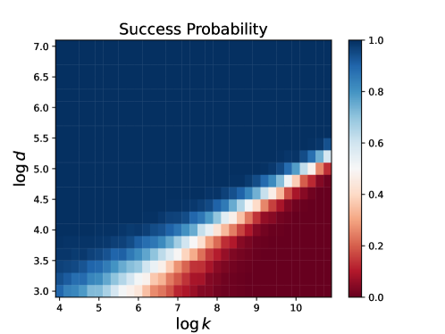
Figure 1: Success probability of tensor power iteration for varying $k$ and $d$.

In our second experiment, we fix $\log k/\log d=1.8$, and varies $d$ and $T$. Again we repeat the experiment 1000 times for each pair of $(d,T)$, and record the estimated success probability after $T$ steps of power iteration. We present the outcomes in Fig. 2. The heatmap shows that polynomially many steps are necessary for tensor power iteration to converge, since $\log T$ scales linearly with $\log d$ around the success/failure boundary. This observation validates Theorem 3.1.

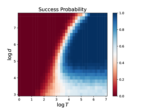
Figure 2: Success probability of tensor power iteration for varying $d$ and $T$.

We illustrate 3.2 in our third experiment. In this experiment, we record the values of the score function $\mathcal{S}$ for the first few iterations along the power iteration path, and compare them with the corresponding theoretical predictions given by 3.2. We repeat such procedure for 1000 times independently, and present the outcomes in Fig. 3, which justifies the correctness of the theorem.

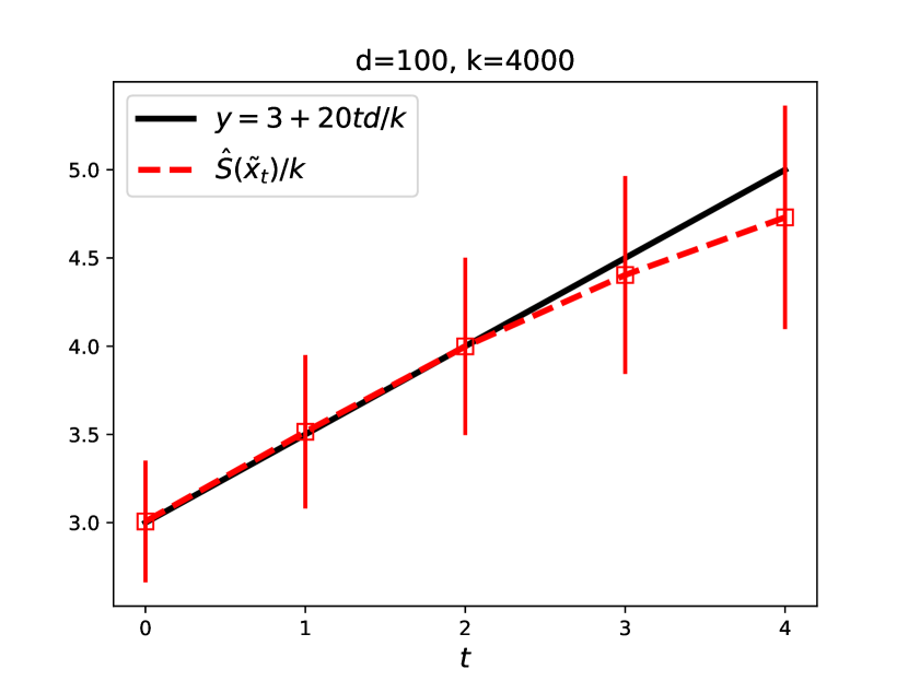
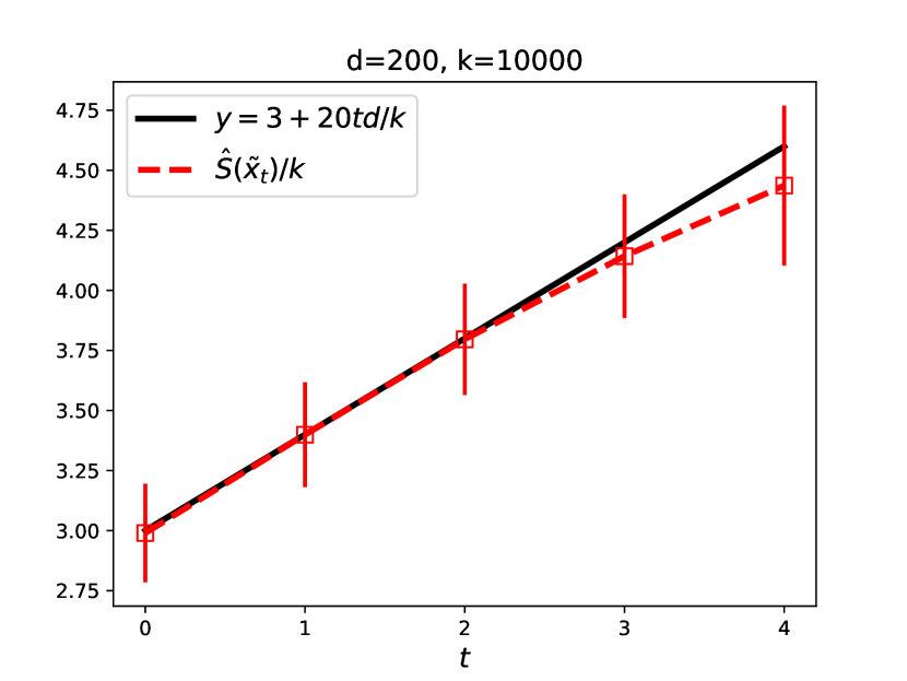
Figure 3: Theoretical predictions of $\mathcal{S}$ along the power iteration paths versus the corresponding empirical values. Outcomes are averaged over 1000 independent experiments. The error bars reflect the intervals determined by two times the empirical standard deviation.

5 Conclusion

We analyze the dynamics of randomly initialized tensor power iteration in the overcomplete regime, using the Gaussian conditioning technique. We prove that it takes polynomially many iterates for the power method to find a true component of a random even-order tensor, thus refuting the previous conjecture that tensor power iteration converges in logarithmically many steps. We also establish that along the power iteration path, a popular polynomial objective function for tensor decomposition is strictly increasing for finitely many steps. Extensive numerical studies verify our theoretical results.

Our work leads to a number of fascinating open problems. First, it would be interesting to understand whether the power method indeed converges to a tensor component in polynomially many steps, within the regime where SOS-based methods succeed. One possible direction is to extend our analysis in Theorem 3.2 to polynomially many iterations. Another appealing direction is to generalize our results to the case of odd-order tensors, for which the power iterates will no longer stay in a small neighborhood of the initialization.

Appendix A Analysis of tensor power iteration: Proof of Theorem 3.1

This section will de devoted to proving 3.1. For $t\in\mathbb{N}_{+}$, we define

$$g_{t}=\sum_{i=1}^{t}\Pi_{F_{1:i-1}}^{\perp}\widetilde{A}_{i}\widetilde{x}^{\perp}_{i-1}\cdot\frac{\langle\widetilde{x}^{\perp}_{i-1},\widetilde{x}_{t-1}\rangle}{\|\widetilde{x}^{\perp}_{i-1}\|_{2}^{2}},$$

$$v_{t}=\sum_{i=2}^{t}f^{\perp}_{i-1}\cdot\frac{\langle x_{i-1},\widetilde{x}^{\perp}_{i-1}\rangle}{\|f^{\perp}_{i-1}\|_{2}^{2}}\cdot\frac{\langle\widetilde{x}^{\perp}_{i-1},\widetilde{x}_{t-1}\rangle}{\|\widetilde{x}^{\perp}_{i-1}\|_{2}^{2}}.$$

By 2.1 we have $y_{t}=g_{t}+v_{t}$. Applying Minkowski’s inequality and power mean inequality, we deduce that $\|y_{t}\|_{4}^{4}\leq 8(\|g_{t}\|_{4}^{4}+\|v_{t}\|_{4}^{4})$. Notice that if Eq. 7 does not hold, since $y_{t}=A\widetilde{x}_{t-1}$, then there exists $1\leq t\leq T$ such that $\|y_{t}\|_{4}^{4}\geq\varepsilon^{4}d^{2}$. As a result, in order to prove 3.1, it suffices to show with high probability, $\|y_{t}\|_{4}^{4}<\varepsilon^{4}d^{2}$ for all $t\in[T]$. This further reduces to upper bounding $\|g_{t}\|_{4}^{4}$ and $\|v_{t}\|_{4}^{4}$.

We first provide an upper bound for $\|g_{t}\|_{4}^{4}$. To this end, we define

$$w_{t}=\sum_{i=1}^{t}\widetilde{A}_{i}\widetilde{x}^{\perp}_{i-1}\cdot\frac{\langle\widetilde{x}^{\perp}_{i-1},\widetilde{x}_{t-1}\rangle}{\|\widetilde{x}^{\perp}_{i-1}\|_{2}^{2}},$$ (9)

$$\eta_{t}=\sum_{i=1}^{t}\sum_{j=1}^{i-1}f^{\perp}_{j}\cdot\frac{\langle f^{\perp}_{j},\widetilde{A}_{i}\widetilde{x}^{\perp}_{i-1}\rangle}{\|f^{\perp}_{j}\|_{2}^{2}}\cdot\frac{\langle\widetilde{x}^{\perp}_{i-1},\widetilde{x}_{t-1}\rangle}{\|\widetilde{x}^{\perp}_{i-1}\|_{2}^{2}}.$$ (10)

We immediately see that $g_{t}=w_{t}-\eta_{t}$, thus upper bounding $\|g_{t}\|_{4}^{4}$ can be achieved via upper bounding $\|w_{t}\|_{4}^{4}$ and $\|\eta_{t}\|_{4}^{4}$, respectively. As $\widetilde{A}_{i}\perp\mathcal{F}_{i-1,i-1}$, intuitively speaking, this suggests that $w_{t}$ behaves like a $k$-dimensional random vector with $\mathrm{i.i.d.}$ standard Gaussian entries. Therefore, with high probability $w_{t}$ has $\ell^{4}$-norm of order $k$. On the other hand, observe that $\eta_{t}$ is the sum of projections of random vectors onto low-dimensional subspaces, which only accounts for a small proportion of the total variation. As a result, we expect $\|\eta_{t}\|_{4}^{4}$ to be small.

To make these heuristic arguments concrete, we establish the following two lemmas:

Lemma A.1.

Assume $T\ll k^{1/2}$. Then there exists a numerical constant $C>0$, such that with probability $1-o_{d}(1)$, for all $1\leq t\leq T$ we have

$$\|w_{t}\|_{4}^{4}\leq Ck.$$

Lemma A.2.

Assume $T\ll k^{1/2}$. Then with probability $1-o_{d}(1)$, for all $1\leq t\leq T$ we have

$$\|\eta_{t}\|_{2}\leq CT^{3/4}(\log k)^{1/4}\frac{\left\|{\Pi_{x_{0}}^{\perp}\widetilde{x}_{t-1}}\right\|_{2}}{\sqrt{d}}.$$

Note that $\|\eta_{t}\|_{4}\leq\|\eta_{t}\|_{2}$. Invoking A.1, A.2, power mean inequality and Minkowski’s inequality, we obtain that with high probability, for all $1\leq t\leq T$,

$$\|g_{t}\|_{4}^{4}\leq 8(\|w_{t}\|_{4}^{4}+\|\eta_{t}\|_{2}^{4})\leq C\left(k+\frac{\left\|{\Pi_{x_{0}}^{\perp}\widetilde{x}_{t-1}}\right\|_{2}^{2}}{d^{2}}\cdot T^{3}\log k\right)\leq C(k+T^{3}\log k)\ll d^{2}$$ (11)

for some numerical constant $C>0$, since under the conditions of 3.1 we have $T\ll d^{1/2}$. Therefore, in order to prove 3.1, it remains to upper bound $\|v_{t+1}\|_{4}^{4}$. In what follows, we perform a crude analysis which uses the $\ell^{2}$-norm to control the $\ell^{4}$-norm. We comment that a more careful analysis might lead to an improved estimate.

The next lemma establishes that the $\ell^{2}$-norm of $v_{t+1}$ is close to the $\ell^{2}$-norm of $\Pi_{x_{0}}^{\perp}(\widetilde{x}_{t})$.

Lemma A.3.

Under the condition of 3.1, with probability $1-o_{d}(1)$, the following result holds for all $0\leq t\leq T-1$:

$$\left(1-\frac{C\log k}{\sqrt{d}}\right)\|\Pi_{x_{0}}^{\perp}(\widetilde{x}_{t})\|_{2}^{2}\leq\|v_{t+1}\|_{2}^{2}\leq\left(1+\frac{C\log k}{\sqrt{d}}\right)\|\Pi_{x_{0}}^{\perp}(\widetilde{x}_{t})\|_{2}^{2}.$$

The rest of the analysis is devoted to upper bounding $\|\Pi_{x_{0}}^{\perp}(\widetilde{x}_{t})\|_{2}^{2}$. By definition, we have

$$\|\Pi_{x_{0}}^{\perp}(\widetilde{x}_{t})\|_{2}^{2}=\frac{d}{\|x_{t}\|_{2}^{2}}\cdot\|\Pi_{x_{0}}^{\perp}(x_{t})\|_{2}^{2}.$$ (12)

Using Eq. 4 we see that

$$x_{t}=\sum_{i=0}^{t-1}\widetilde{x}^{\perp}_{i}\cdot\frac{\langle h_{i+1},f_{t}\rangle}{\|\widetilde{x}^{\perp}_{i}\|_{2}^{2}}+\Pi_{X_{0:t-1}}^{\perp}\overline{A}_{t}^{{\sf T}}f^{\perp}_{t},$$

$$\Pi_{x_{0}}^{\perp}(x_{t})=\sum_{i=1}^{t-1}\widetilde{x}^{\perp}_{i}\cdot\frac{\langle h_{i+1},f_{t}\rangle}{\|\widetilde{x}^{\perp}_{i}\|_{2}^{2}}+\Pi_{X_{0:t-1}}^{\perp}\overline{A}_{t}^{{\sf T}}f^{\perp}_{t}.$$

According to Pythagorean theorem,

$$\|x_{t}\|_{2}^{2}=\sum_{i=0}^{t-1}\frac{\langle h_{i+1},f_{t}\rangle^{2}}{\|\widetilde{x}^{\perp}_{i}\|_{2}^{2}}+\|\Pi_{X_{0:t-1}}^{\perp}\overline{A}_{t}^{{\sf T}}f^{\perp}_{t}\|_{2}^{2},$$ (13)

$$\|\Pi_{x_{0}}^{\perp}(x_{t})\|_{2}^{2}=\sum_{i=1}^{t-1}\frac{\langle h_{i+1},f_{t}\rangle^{2}}{\|\widetilde{x}^{\perp}_{i}\|_{2}^{2}}+\|\Pi_{X_{0:t-1}}^{\perp}\overline{A}_{t}^{{\sf T}}f^{\perp}_{t}\|_{2}^{2}.$$ (14)

Using the definition of $h_{i+1}$ given in Eq. 6, we deduce that

$$\frac{\langle h_{i+1},f_{t}\rangle}{\|\widetilde{x}^{\perp}_{i}\|_{2}}=\frac{\langle f^{\perp}_{i},f_{t}\rangle}{\|\widetilde{x}^{\perp}_{i}\|_{2}}\cdot\frac{\langle x_{i},\widetilde{x}^{\perp}_{i}\rangle}{\|f^{\perp}_{i}\|_{2}^{2}}+\frac{\langle\Pi_{F_{1:i}}^{\perp}\widetilde{A}_{i+1}\widetilde{x}^{\perp}_{i},f_{t}\rangle}{\|\widetilde{x}^{\perp}_{i}\|_{2}}.$$ (15)

Combining Eqs. 13, 14 and 15, we obtain the following decomposition:

$$\begin{split}&\|x_{t}\|_{2}^{2}=\mathsf{I}+\mathsf{II}+\mathsf{III},\\ &\|\Pi_{x_{0}}^{\perp}(x_{t})\|_{2}^{2}=\mathsf{I}^{\prime}+\mathsf{II}+\mathsf{III},\end{split}$$ (16)

where

$$\mathsf{I}=\sum_{i=0}^{t-1}\frac{\langle\Pi_{F_{1:i}}^{\perp}\widetilde{A}_{i+1}\widetilde{x}^{\perp}_{i},f_{t}\rangle^{2}}{\|\widetilde{x}^{\perp}_{i}\|_{2}^{2}},\qquad\mathsf{I}^{\prime}=\sum_{i=1}^{t-1}\frac{\langle\Pi_{F_{1:i}}^{\perp}\widetilde{A}_{i+1}\widetilde{x}^{\perp}_{i},f_{t}\rangle^{2}}{\|\widetilde{x}^{\perp}_{i}\|_{2}^{2}},$$ (17)

$$\mathsf{II}=\sum_{i=1}^{t-1}\frac{\langle f^{\perp}_{i},f_{t}\rangle^{2}}{\|f^{\perp}_{i}\|_{2}^{2}}\cdot\frac{\langle x_{i},x^{\perp}_{i}\rangle}{\|f^{\perp}_{i}\|_{2}^{2}}+\|\Pi_{X_{0:t-1}}^{\perp}\overline{A}_{t}^{{\sf T}}f^{\perp}_{t}\|_{2}^{2},$$ (18)

$$\mathsf{III}=\sum_{i=1}^{t-1}\frac{2\langle x_{i},\widetilde{x}^{\perp}_{i}\rangle\langle f^{\perp}_{i},f_{t}\rangle\langle\Pi_{F_{1:i}}^{\perp}\widetilde{A}_{i+1}\widetilde{x}^{\perp}_{i},f_{t}\rangle}{\|\widetilde{x}^{\perp}_{i}\|_{2}^{2}\|f^{\perp}_{i}\|_{2}^{2}}.$$ (19)

Next, we will show that terms $\mathsf{II}$ and $\mathsf{III}$ are negligible comparing to terms $\mathsf{I}$ and $\mathsf{I}^{\prime}$. Note that by Cauchy-Schwarz inequality, $|\mathsf{III}|\leq 2\sqrt{\mathsf{I}^{\prime}\times\mathsf{II}}$, namely the term $\mathsf{III}$ is controlled by $\mathsf{II}$. This motivates us to first provide an upper bound for term $\mathsf{II}$.

Lemma A.4.

Under the condition of 3.1, with probability $1-o_{d}(1)$, for all $1\leq t\leq T$ we have (note that $\mathsf{II}$ depends on $t$ as well)

$$\left(1-\frac{C\log k}{\sqrt{d}}\right)\|f_{t}\|_{2}^{2}\leq\mathsf{II}\leq\left(1+\frac{C\log k}{\sqrt{d}}\right)\|f_{t}\|_{2}^{2}.$$

The following lemma establishes an upper bound on $\|f_{t}\|_{2}^{2}$:

Lemma A.5.

Under the condition of 3.1, there exists a numerical constant $C>0$, such that with probability $1-o_{d}(1)$, for all $1\leq t\leq T$ we have

$$\left\|{f_{t}}\right\|_{2}^{2}\leq C\left(k+\|\Pi_{x_{0}}^{\perp}(\widetilde{x}_{t-1})\|_{2}^{6}\right).$$

With the aid of A.4 and A.5, we obtain that with high probability

$$\mathsf{II}\leq C\left(k+\|\Pi_{x_{0}}^{\perp}(\widetilde{x}_{t-1})\|_{2}^{6}\right)$$

for all $1\leq t\leq T$ and some positive numerical constant $C$. Next, we analyze terms $\mathsf{I}$ and $\mathsf{I}^{\prime}$. To achieve this goal, we find the following lemma useful:

Lemma A.6.

Under the condition of 3.1, there exists a numerical constant $C>0$, such that with probability $1-o_{d}(1)$, for all $0\leq i<t\leq T$, we have

$$\left|\frac{\langle\Pi_{F_{1:i}}^{\perp}\widetilde{A}_{i+1}\widetilde{x}^{\perp}_{i},f_{t}\rangle}{\|\widetilde{x}^{\perp}_{i}\|_{2}}-\frac{3k}{d}\cdot\frac{\langle\widetilde{x}^{\perp}_{i},\widetilde{x}_{t-1}\rangle}{\|\widetilde{x}^{\perp}_{i}\|_{2}}\right|$$

$$\leq\, C\left(\sqrt{\frac{kT\log k}{d}}+\sqrt{\frac{T}{d}}\,\|\Pi_{x_{0}}^{\perp}(\widetilde{x}_{t-1})\|_{2}^{3}+\sqrt{\frac{k\log k}{d}}\,\|\Pi_{x_{0}}^{\perp}\widetilde{x}_{t-1}\|_{2}\right).$$

Now we are in position to finish the proof of 3.1. For future convenience, we hereby establish a general framework for the analysis of tensor power iteration dynamics, based on A.1 to A.6. To begin with, let us denote

$$P_{t}=\left\|{\Pi_{x_{0}}^{\perp}(\widetilde{x}_{t})}\right\|_{2}^{2},\quad Q_{t}=\left\|{\Pi_{x_{0}}(\widetilde{x}_{t})}\right\|_{2}^{2}.$$

Then, we know that $P_{t}+Q_{t}=\left\|{\widetilde{x}_{t}}\right\|_{2}^{2}=d$, and that

$$\frac{P_{t}}{Q_{t}}=\frac{\left\|{\Pi_{x_{0}}^{\perp}(x_{t})}\right\|_{2}^{2}}{\left\|{\Pi_{x_{0}}(x_{t})}\right\|_{2}^{2}}=\frac{\mathsf{I}^{\prime}+\mathsf{II}+\mathsf{III}}{\mathsf{I}-\mathsf{I}^{\prime}}.$$

Recall that our aim is to show that $\left\|{v_{t}}\right\|_{2}^{4}\ll d^{2}$ for all $1\leq t\leq T$. According to A.3, this amounts to proving that $P_{t}\ll Q_{t}$ for all $t\in[T]$. Define the stopping time

$$T_{k}=\inf\{t\in\mathbb{N}_{+}:P_{t}\geq k^{1/3}\}.$$

Since $k^{1/3}\ll d$, it then suffices to show that $T_{k}\geq T(k,d)$ with high probability, where $T(k,d)$ is defined in the statement of Theorem 3.1.

Step 1. A lower bound for $\mathsf{I}-\mathsf{I}^{\prime}$. By definition, we know that

$$\mathsf{I}-\mathsf{I}^{\prime}=\frac{\langle\widetilde{A}_{1}\widetilde{x}_{0},f_{t}\rangle^{2}}{\left\|{\widetilde{x}_{0}}\right\|_{2}^{2}}.$$

Note that the proof of A.6 also implies that

$$\left|\frac{\langle\widetilde{A}_{1}\widetilde{x}_{0},f_{t}\rangle}{\|\widetilde{x}_{0}\|_{2}}-\frac{3k}{d}\sqrt{Q_{t-1}}\right|\leq\, C\left(\sqrt{\frac{kT\log k}{d}}+\sqrt{\frac{\log k}{d}}\,\|\Pi_{x_{0}}^{\perp}(\widetilde{x}_{t-1})\|_{2}^{3}+\sqrt{\frac{k\log k}{d}}\,\|\Pi_{x_{0}}^{\perp}\widetilde{x}_{t-1}\|_{2}\right)$$

$$=\, C\left(\sqrt{\frac{kT\log k}{d}}+\sqrt{\frac{\log k}{d}}\,P_{t-1}^{3/2}+\sqrt{\frac{k\log k}{d}}\,P_{t-1}^{1/2}\right)$$

$$=\, C(\log k)^{1/2}\left(\sqrt{\frac{kT}{d}}+\frac{1}{\sqrt{d}}\,P_{t-1}^{3/2}+\sqrt{\frac{k}{d}}\,P_{t-1}^{1/2}\right).$$

For $t\leq T_{k}$, we have $Q_{t-1}\asymp d$, thus leading to the estimate:

$$\mathsf{I}-\mathsf{I}^{\prime}=\frac{\langle\widetilde{A}_{1}\widetilde{x}_{0},f_{t}\rangle^{2}}{\left\|{\widetilde{x}_{0}}\right\|_{2}^{2}}\geq\, \frac{9k^{2}}{d^{2}}Q_{t-1}\cdot\left(1-\frac{C(\log k)^{1/2}\left(\sqrt{dkT}+\sqrt{d}\,P_{t-1}^{3/2}+\sqrt{dk}\,P_{t-1}^{1/2}\right)}{3k\sqrt{Q_{t-1}}}\right)^{2}$$

$$\geq\, \frac{9k^{2}}{d^{2}}Q_{t-1}\cdot\left(1-C(\log k)^{1/2}\left(k^{-1/2}\,T^{1/2}+k^{-1}P_{t-1}^{3/2}+k^{-1/2}\,P_{t-1}^{1/2}\right)\right)^{2}.$$

Hence, it follows that

$$\frac{1}{\mathsf{I}-\mathsf{I}^{\prime}}\leq\frac{d^{2}}{9k^{2}Q_{t-1}}\cdot\left(1+C(\log k)^{1/2}\left(k^{-1/2}\,T^{1/2}+k^{-1}P_{t-1}^{3/2}+k^{-1/2}\,P_{t-1}^{1/2}\right)\right),$$

where the last line is due to the fact that

$$(\log k)^{1/2}\left(k^{-1/2}\,T^{1/2}+k^{-1}P_{t-1}^{3/2}+k^{-1/2}\,P_{t-1}^{1/2}\right)=o(1).$$

Since by our assumption, $T\ll k^{1/3}$, and $P_{t-1}\leq k^{1/3}$.

Step 2. An upper bound for $\mathsf{I}^{\prime}+\mathsf{II}+\mathsf{III}$. Using Cauchy-Schwarz inequality, we get

$$\mathsf{I}^{\prime}+\mathsf{II}+\mathsf{III}\leq\mathsf{I}^{\prime}+\mathsf{II}+2\sqrt{\mathsf{I}^{\prime}\times\mathsf{II}}=\left(\sqrt{\mathsf{I}^{\prime}}+\sqrt{\mathsf{II}}\right)^{2}.$$

To upper bound $\sqrt{\mathsf{I}^{\prime}}$, we note that

$$\left|\sqrt{\mathsf{I}^{\prime}}-\frac{3k}{d}\sqrt{P_{t-1}}\right|=\frac{|\mathsf{I}^{\prime}-9k^{2}P_{t-1}/d^{2}|}{\sqrt{\mathsf{I}^{\prime}}+3k\sqrt{P_{t-1}}/d}$$

$$\leq\, \frac{1}{\sqrt{\mathsf{I}^{\prime}}+3k\sqrt{P_{t-1}}/d}\cdot\left|\sum_{i=1}^{t-1}\frac{\langle\Pi_{F_{1:i}}^{\perp}\widetilde{A}_{i+1}\widetilde{x}^{\perp}_{i},f_{t}\rangle^{2}}{\|\widetilde{x}^{\perp}_{i}\|_{2}^{2}}-\frac{9k^{2}}{d^{2}}\sum_{i=1}^{t-1}\frac{\langle\widetilde{x}^{\perp}_{i},\widetilde{x}_{t-1}\rangle^{2}}{\|\widetilde{x}^{\perp}_{i}\|_{2}^{2}}\right|$$

$$=\, \frac{1}{\sqrt{\mathsf{I}^{\prime}}+3k\sqrt{P_{t-1}}/d}\cdot\left|\sum_{i=1}^{t-1}\left(\frac{\langle\Pi_{F_{1:i}}^{\perp}\widetilde{A}_{i+1}\widetilde{x}^{\perp}_{i},f_{t}\rangle}{\|\widetilde{x}^{\perp}_{i}\|_{2}}-\frac{3k}{d}\frac{\langle\widetilde{x}^{\perp}_{i},\widetilde{x}_{t-1}\rangle}{\|\widetilde{x}^{\perp}_{i}\|_{2}}\right)\left(\frac{\langle\Pi_{F_{1:i}}^{\perp}\widetilde{A}_{i+1}\widetilde{x}^{\perp}_{i},f_{t}\rangle}{\|\widetilde{x}^{\perp}_{i}\|_{2}}+\frac{3k}{d}\frac{\langle\widetilde{x}^{\perp}_{i},\widetilde{x}_{t-1}\rangle}{\|\widetilde{x}^{\perp}_{i}\|_{2}}\right)\right|$$

$$\leq\, \frac{1}{\sqrt{\mathsf{I}^{\prime}}+3k\sqrt{P_{t-1}}/d}\cdot\sqrt{\sum_{i=1}^{t-1}\left(\frac{\langle\Pi_{F_{1:i}}^{\perp}\widetilde{A}_{i+1}\widetilde{x}^{\perp}_{i},f_{t}\rangle}{\|\widetilde{x}^{\perp}_{i}\|_{2}}-\frac{3k}{d}\frac{\langle\widetilde{x}^{\perp}_{i},\widetilde{x}_{t-1}\rangle}{\|\widetilde{x}^{\perp}_{i}\|_{2}}\right)^{2}}$$

$$\times\sqrt{\sum_{i=1}^{t-1}\left(\frac{\langle\Pi_{F_{1:i}}^{\perp}\widetilde{A}_{i+1}\widetilde{x}^{\perp}_{i},f_{t}\rangle}{\|\widetilde{x}^{\perp}_{i}\|_{2}}+\frac{3k}{d}\frac{\langle\widetilde{x}^{\perp}_{i},\widetilde{x}_{t-1}\rangle}{\|\widetilde{x}^{\perp}_{i}\|_{2}}\right)^{2}}$$

$$\stackrel{{\scriptstyle(i)}}{{\leq}}\, C\sqrt{\sum_{i=1}^{t-1}\left(\frac{\langle\Pi_{F_{1:i}}^{\perp}\widetilde{A}_{i+1}\widetilde{x}^{\perp}_{i},f_{t}\rangle}{\|\widetilde{x}^{\perp}_{i}\|_{2}}-\frac{3k}{d}\frac{\langle\widetilde{x}^{\perp}_{i},\widetilde{x}_{t-1}\rangle}{\|\widetilde{x}^{\perp}_{i}\|_{2}}\right)^{2}}$$

$$\stackrel{{\scriptstyle(ii)}}{{\leq}}\, C\left(\sqrt{\frac{k\log k}{d}}\,T+\sqrt{\frac{T^{2}}{d}}\,\|\Pi_{x_{0}}^{\perp}(\widetilde{x}_{t-1})\|_{2}^{3}+\sqrt{\frac{Tk\log k}{d}}\,\|\Pi_{x_{0}}^{\perp}\widetilde{x}_{t-1}\|_{2}\right)$$

$$\leq\, C(\log k)^{1/2}\left(\sqrt{\frac{k}{d}}\,T+\frac{T}{\sqrt{d}}\,P_{t-1}^{3/2}+\sqrt{\frac{Tk}{d}}\,P_{t-1}^{1/2}\right),$$

where $(i)$ follows from Minkowski’s inequality, and $(ii)$ follows from A.6. Using A.4 and A.5, we obtain that with high probability,

$$\sqrt{\mathsf{II}}\leq C\left\|{f_{t}}\right\|_{2}\leq C\left(\sqrt{k}+\|\Pi_{x_{0}}^{\perp}(\widetilde{x}_{t-1})\|_{2}^{3}\right)=C\left(\sqrt{k}+P_{t-1}^{3/2}\right),$$

thus leading to the estimate:

$$\sqrt{\mathsf{I}^{\prime}}+\sqrt{\mathsf{II}}\leq\frac{3k}{d}\sqrt{P_{t-1}}+C(\log k)^{1/2}\left(\sqrt{\frac{k}{d}}\,T+\sqrt{\frac{Tk}{d}}\,P_{t-1}^{1/2}\right)+C\left(\sqrt{k}+P_{t-1}^{3/2}\right),$$

since $T\ll d^{1/3}$ by our assumption. We finally obtain that

$$\mathsf{I}^{\prime}+\mathsf{II}+\mathsf{III}\leq\, \left(\frac{3k}{d}\sqrt{P_{t-1}}+C(\log k)^{1/2}\left(\sqrt{\frac{k}{d}}\,T+\sqrt{\frac{Tk}{d}}\,P_{t-1}^{1/2}\right)+C\left(\sqrt{k}+P_{t-1}^{3/2}\right)\right)^{2}$$

$$\leq\, \left(\frac{3k}{d}\sqrt{P_{t-1}}+C(\log k)^{1/2}\sqrt{\frac{Tk}{d}}\,P_{t-1}^{1/2}+C\left(\sqrt{k}+P_{t-1}^{3/2}\right)\right)^{2}.$$

Step 3. Write a recurrence inequality for $P_{t}/Q_{t}$. Combining our results from the previous steps gives the following recurrence relationship:

$$\frac{P_{t}}{Q_{t}}=\frac{\mathsf{I}^{\prime}+\mathsf{II}+\mathsf{III}}{\mathsf{I}-\mathsf{I}^{\prime}}\leq\, \frac{d^{2}}{9k^{2}Q_{t-1}}\cdot\left(\frac{3k}{d}\sqrt{P_{t-1}}+C(\log k)^{1/2}\sqrt{\frac{Tk}{d}}\,P_{t-1}^{1/2}+C\left(\sqrt{k}+P_{t-1}^{3/2}\right)\right)^{2}$$

$$\times\left(1+C(\log k)^{1/2}\left(k^{-1/2}\,T^{1/2}+k^{-1}P_{t-1}^{3/2}+k^{-1/2}\,P_{t-1}^{1/2}\right)\right).$$

Denote the right hand side of the above inequality as $U_{k,d,T}(P_{t-1}/Q_{t-1})$, then we know that $U_{k,d,T}$ is an increasing function: As $P_{t-1}/Q_{t-1}$ increases, $P_{t-1}$ increases and $Q_{t-1}$ decreases. Hence, the right hand side of the above inequality will also increase. As a consequence, we deduce that

$$\frac{P_{T}}{Q_{T}}\leq U_{k,d,T}^{T}\left(\frac{P_{0}}{Q_{0}}\right)=U_{k,d,T}^{T}\left(0\right)\leq U_{k,d,T}^{T}\left(\frac{k^{1/3}/2}{d-k^{1/3}/2}\right).$$

By definition of $U_{k,d,T}$, whenever

$$\frac{k^{1/3}/2}{d-k^{1/3}/2}\leq x\leq\frac{k^{1/3}}{d-k^{1/3}},$$

we have the following estimate:

$$U_{k,d,T}\left(x\right)\leq\, x\times\left(1+2C\cdot\frac{d}{k^{2/3}}+C(\log k)^{1/2}\cdot\frac{d^{1/2}T^{1/2}}{k^{1/2}}\right)^{2}$$

$$\times\left(1+C(\log k)^{1/2}\left(\frac{T^{1/2}}{k^{1/2}}+2k^{-1/3}\right)\right)$$

$$\stackrel{{\scriptstyle(i)}}{{\leq}}\, \left(1+\frac{Cd}{k^{2/3}}+C(\log k)^{1/2}\left(\frac{d^{1/2}T^{1/2}}{k^{1/2}}+k^{-1/3}\right)\right)\cdot x$$

$$\stackrel{{\scriptstyle(ii)}}{{\leq}}\, \left(1+\frac{Cd}{k^{2/3}}+C(\log k)^{1/2}\cdot\frac{d^{1/2}T^{1/2}}{k^{1/2}}\right)\cdot x,$$

where $(i)$ and $(ii)$ both follow from our assumption: $d^{3/2}\ll k\ll d^{2}$. Since $k^{1/3}\ll d$, it suffices to show that for $T=T(k,d)\ll(\log k)^{-1/3}\cdot(k^{2/3}/d)$,

$$U_{k,d,T}^{T}\left(\frac{k^{1/3}/2}{d-k^{1/3}/2}\right)\leq\frac{k^{1/3}}{d-k^{1/3}}.$$

Let $T^{\prime}$ be the maximum integer such that

$$U_{k,d,T}^{T^{\prime}}\left(\frac{k^{1/3}/2}{d-k^{1/3}/2}\right)\leq\frac{k^{1/3}}{d-k^{1/3}},$$

then by monotonicity of $U_{k,d,T}$ and maximality of $T^{\prime}$ we know that

$$\frac{k^{1/3}}{d-k^{1/3}}<U_{k,d,T}^{T^{\prime}+1}\left(\frac{k^{1/3}/2}{d-k^{1/3}/2}\right)\leq\, \left(1+\frac{Cd}{k^{2/3}}+C(\log k)^{1/2}\cdot\frac{d^{1/2}T^{1/2}}{k^{1/2}}\right)^{T^{\prime}+1}\times\frac{k^{1/3}/2}{d-k^{1/3}/2}$$

$$\leq\, \exp\left(C(T^{\prime}+1)\left(\frac{d}{k^{2/3}}+(\log k)^{1/2}\cdot\frac{d^{1/2}T^{1/2}}{k^{1/2}}\right)\right)\times\frac{k^{1/3}/2}{d-k^{1/3}/2},$$

which further implies that

$$T^{\prime}+1\geq\, (\log 2/C)\cdot\left(\frac{d}{k^{2/3}}+(\log k)^{1/2}\cdot\frac{d^{1/2}T^{1/2}}{k^{1/2}}\right)^{-1}\geq\frac{\log 2}{2C}\cdot\min\left\{\frac{k^{2/3}}{d},\ (\log k)^{-1/3}k^{1/6}\right\}$$

$$\geq\, \frac{\log 2}{2C}\cdot(\log k)^{-1/3}\cdot\frac{k^{2/3}}{d}\implies T^{\prime}\gtrsim(\log k)^{-1/3}\cdot\frac{k^{2/3}}{d}.$$

This completes the proof of 3.1.

A.1 Proof of Lemma A.1

For $i,t\in[T]$, we define

$$z_{i}=\widetilde{A}_{i}\widetilde{x}^{\perp}_{i-1}\cdot\frac{\sqrt{d}}{\|\widetilde{x}^{\perp}_{i-1}\|_{2}},\qquad\alpha_{i,t}=\frac{\langle\widetilde{x}^{\perp}_{i-1},\widetilde{x}_{t-1}\rangle}{\sqrt{d}\|\widetilde{x}^{\perp}_{i-1}\|_{2}}.$$ (20)

We immediately see that for all $t\in[T]$, we have $\sum_{i=1}^{t}\alpha_{i,t}^{2}=1$, and that $w_{t}=\sum_{i=1}^{t}\alpha_{i,t}z_{i}$. According to 2.1, for all $i\in[T]$ we have $\widetilde{A}_{i}\perp\sigma(\mathcal{F}_{i-1,i-1}\cup\sigma(\overline{A}_{1},\cdots,\overline{A}_{i-1},\widetilde{A}_{1},\cdots,\widetilde{A}_{i-1}))$, we then obtain that for any $i\in[T]$ and $\{z_{1},\cdots,z_{i-1}\}$, $z_{i}\mid z_{1},\cdots,z_{i-1}\overset{d}{=}{\sf N}(0,I_{k})$. As a result, we see that $z_{1},\cdots,z_{T}$ are independent and identically distributed random vectors with marginal distribution ${\sf N}(0,I_{k})$. Hence, it suffices to prove that

$$\sup_{\alpha\in\mathbb{S}^{T-1}}\left\|{\sum_{i=1}^{T}\alpha_{i}z_{i}}\right\|_{4}^{4}\leq Ck$$

with high probability. To this end, we use a covering argument. Fix $\varepsilon\in(0,1)$ (to be determined later), let $N_{\varepsilon}(\mathbb{S}^{T-1})$ be an $\varepsilon$-covering of $\mathbb{S}^{T-1}$. Then for any $\alpha\in\mathbb{S}^{T-1}$, there exists $\alpha^{\prime}\in N_{\varepsilon}(\mathbb{S}^{T-1})$ such that $\left\|{\alpha-\alpha^{\prime}}\right\|_{2}\leq\varepsilon$, thus leading to

$$\left\|{\sum_{i=1}^{T}\alpha_{i}z_{i}}\right\|_{4}\leq\left\|{\sum_{i=1}^{T}\alpha^{\prime}_{i}z_{i}}\right\|_{4}+\left\|{\sum_{i=1}^{T}(\alpha_{i}-\alpha^{\prime}_{i})z_{i}}\right\|_{4}\leq\sup_{\alpha\in N_{\varepsilon}(\mathbb{S}^{T-1})}\left\|{\sum_{i=1}^{T}\alpha_{i}z_{i}}\right\|_{4}+\varepsilon\cdot\sup_{\alpha\in\mathbb{S}^{T-1}}\left\|{\sum_{i=1}^{T}\alpha_{i}z_{i}}\right\|_{4},$$

which further implies that

$$\sup_{\alpha\in\mathbb{S}^{T-1}}\left\|{\sum_{i=1}^{T}\alpha_{i}z_{i}}\right\|_{4}\leq\sup_{\alpha\in N_{\varepsilon}(\mathbb{S}^{T-1})}\left\|{\sum_{i=1}^{T}\alpha_{i}z_{i}}\right\|_{4}+\varepsilon\cdot\sup_{\alpha\in\mathbb{S}^{T-1}}\left\|{\sum_{i=1}^{T}\alpha_{i}z_{i}}\right\|_{4}$$

$$\implies\, \sup_{\alpha\in\mathbb{S}^{T-1}}\left\|{\sum_{i=1}^{T}\alpha_{i}z_{i}}\right\|_{4}\leq\frac{1}{1-\varepsilon}\cdot\sup_{\alpha\in N_{\varepsilon}(\mathbb{S}^{T-1})}\left\|{\sum_{i=1}^{T}\alpha_{i}z_{i}}\right\|_{4}.$$

Now, for any fixed $\alpha\in N_{\varepsilon}(\mathbb{S}^{T-1})$, we know that $\sum_{i=1}^{T}\alpha_{i}z_{i}\sim\mathsf{N}(0,I_{k})$. According to Lemma D.3, we know that there exists a constant $C>0$ such that

$$\mathbb{P}\left(\left\|{\sum_{i=1}^{T}\alpha_{i}z_{i}}\right\|_{4}^{4}\geq Ck\right)\leq C\exp(-Ck^{1/2}).$$

Applying a union bound then gives

$$\mathbb{P}\left(\sup_{\alpha\in N_{\varepsilon}(\mathbb{S}^{T-1})}\left\|{\sum_{i=1}^{T}\alpha_{i}z_{i}}\right\|_{4}^{4}\geq Ck\right)\leq C\left(\frac{C}{\varepsilon}\right)^{T}\exp(-Ck^{1/2}).$$

By our assumption, $T\ll k^{1/2}$. Now we choose $\varepsilon=1/2$, it follows that

$$\sup_{\alpha\in\mathbb{S}^{T-1}}\left\|{\sum_{i=1}^{T}\alpha_{i}z_{i}}\right\|_{4}^{4}\leq 2^{4}\cdot\sup_{\alpha\in N_{\varepsilon}(\mathbb{S}^{T-1})}\left\|{\sum_{i=1}^{T}\alpha_{i}z_{i}}\right\|_{4}^{4}\leq Ck$$

with high probability. This completes the proof of Lemma A.1.

A.2 Proof of Lemma A.2

Recall the definition of $\eta_{t}$ from Eq. 10:

$$\eta_{t}=\sum_{i=1}^{t}\sum_{j=1}^{i-1}f^{\perp}_{j}\cdot\frac{\langle f^{\perp}_{j},\widetilde{A}_{i}\widetilde{x}^{\perp}_{i-1}\rangle}{\|f^{\perp}_{j}\|_{2}^{2}}\cdot\frac{\langle\widetilde{x}^{\perp}_{i-1},\widetilde{x}_{t-1}\rangle}{\|\widetilde{x}^{\perp}_{i-1}\|_{2}^{2}}=\sum_{i=1}^{t}\alpha_{i,t}\Pi_{F_{1:i-1}}z_{i}=\sum_{i=2}^{t}\alpha_{i,t}\Pi_{F_{1:i-1}}z_{i},$$

where the last equality follows from the fact that $\Pi_{F_{1:0}}=0$, and the $\alpha_{i,t}$’s and $z_{i}$’s are defined in the proof of A.1. We thus obtain that

$$\left\|{\eta_{t}}\right\|_{2}^{2}=\sum_{i=2}^{t}\sum_{j=2}^{t}\alpha_{i,t}\alpha_{j,t}\left\langle\Pi_{F_{1:i-1}}z_{i},\Pi_{F_{1:j-1}}z_{j}\right\rangle$$

$$\leq\, \sum_{i=2}^{t}\alpha_{i,t}^{2}\left\|{\Pi_{F_{1:i-1}}z_{i}}\right\|_{2}^{2}+2\sum_{2\leq i<j\leq t}\left|\alpha_{i,t}\alpha_{j,t}\left\langle\Pi_{F_{1:i-1}}z_{i},\Pi_{F_{1:j-1}}z_{j}\right\rangle\right|,$$

where for $i<j$, we know that

$$\left\langle\Pi_{F_{1:i-1}}z_{i},\Pi_{F_{1:j-1}}z_{j}\right\rangle=z_{j}^{\sf T}\Pi_{F_{1:j-1}}\Pi_{F_{1:i-1}}z_{i}=z_{j}^{\sf T}\Pi_{F_{1:i-1}}z_{i}=\mathrm{Tr}\left(\Pi_{F_{1:i-1}}z_{i}z_{j}^{\sf T}\right).$$

Using the same argument as in the proof of A.1, we see that for $i<j$, $\Pi_{F_{1:i-1}}$, $z_{i}\sim\mathsf{N}(0,I_{k})$, and $z_{j}\sim\mathsf{N}(0,I_{k})$ are mutually independent. In fact, given $(\Pi_{F_{1:i-1}},z_{i})$, the conditional distribution of $z_{j}$ is always $\mathsf{N}(0,I_{k})$, and given $\Pi_{F_{1:i-1}}$, the conditional distribution of $z_{i}$ is always $\mathsf{N}(0,I_{k})$. This further implies that

$$\mathbb{P}\left(\left|z_{j}^{\sf T}\Pi_{F_{1:i-1}}z_{i}\right|\geq\sqrt{C\log k}\left\|{\Pi_{F_{1:i-1}}z_{i}}\right\|_{2}\big{|}(\Pi_{F_{1:i-1}},z_{i})\right)\leq\,k^{-C},$$

$$\mathbb{P}\left(\left\|{\Pi_{F_{1:i-1}}z_{i}}\right\|_{2}\geq\sqrt{CT}\right)\leq\,C\exp(-CT),$$

where $C>0$ is an absolute constant. Therefore, we conclude that with probability $1-o_{d}(1)$, for all $2\leq i<j\leq T$, one has

$$\left|\left\langle\Pi_{F_{1:i-1}}z_{i},\Pi_{F_{1:j-1}}z_{j}\right\rangle\right|\leq\sqrt{CT\log k},\ \left\|{\Pi_{F_{1:i-1}}z_{i}}\right\|_{2}^{2}\leq CT,$$

thus leading to the following estimate:

$$\left\|{\eta_{t}}\right\|_{2}^{2}\leq\, CT\sum_{i=2}^{t}\alpha_{i,t}^{2}+2\sqrt{CT\log k}\sum_{2\leq i<j\leq t}\left|\alpha_{i,t}\alpha_{j,t}\right|\leq CT\left(1-\alpha_{1,t}^{2}\right)+\sqrt{CT\log k}\left(\sum_{i=2}^{t}\left|\alpha_{i,t}\right|\right)^{2}$$

$$\leq\, CT\left(1-\alpha_{1,t}^{2}\right)+t\sqrt{CT\log k}\cdot\sum_{i=2}^{t}\alpha_{i,t}^{2}\leq CT^{3/2}(\log k)^{1/2}\left(1-\alpha_{1,t}^{2}\right).$$

Note that by definition, we have

$$1-\alpha_{1,t}^{2}=1-\frac{\langle\widetilde{x}_{0}^{\perp},\widetilde{x}_{t-1}\rangle^{2}}{d\left\|{\widetilde{x}_{0}^{\perp}}\right\|_{2}^{2}}=1-\frac{1}{d}\left\|{\Pi_{x_{0}}\widetilde{x}_{t-1}}\right\|_{2}^{2}=\frac{1}{d}\left\|{\Pi_{x_{0}}^{\perp}\widetilde{x}_{t-1}}\right\|_{2}^{2}.$$

Hence, we finally deduce that with high probability,

$$\left\|{\eta_{t}}\right\|_{2}\leq CT^{3/4}(\log k)^{1/4}\frac{\left\|{\Pi_{x_{0}}^{\perp}\widetilde{x}_{t-1}}\right\|_{2}}{\sqrt{d}}$$

for all $t\in[T]$, as desired. This concludes the proof.

A.3 Proof of Lemma A.3

Recall the definition of $v_{t+1}$:

$$v_{t+1}=\sum_{i=1}^{t}f_{i}^{\perp}\cdot\frac{\langle x_{i},\widetilde{x}_{i}^{\perp}\rangle}{\left\|{f_{i}^{\perp}}\right\|_{2}^{2}}\cdot\frac{\langle\widetilde{x}_{i}^{\perp},\widetilde{x}_{t}\rangle}{\left\|{\widetilde{x}_{i}^{\perp}}\right\|_{2}^{2}}.$$

Since $\{f_{i}^{\perp}\}_{1\leq i\leq t}$ is an orthogonal set, we readily see that

$$\left\|{v_{t+1}}\right\|_{2}^{2}=\, \sum_{i=1}^{t}\frac{\langle x_{i},\widetilde{x}_{i}^{\perp}\rangle^{2}}{\left\|{f_{i}^{\perp}}\right\|_{2}^{2}}\cdot\frac{\langle\widetilde{x}_{i}^{\perp},\widetilde{x}_{t}\rangle^{2}}{\left\|{\widetilde{x}_{i}^{\perp}}\right\|_{2}^{4}}=\sum_{i=1}^{t}\frac{\left\|{x_{i}}\right\|_{2}^{2}}{d}\cdot\frac{\langle\widetilde{x}_{i},\widetilde{x}_{i}^{\perp}\rangle^{2}}{\left\|{f_{i}^{\perp}}\right\|_{2}^{2}}\cdot\frac{\langle\widetilde{x}_{i}^{\perp},\widetilde{x}_{t}\rangle^{2}}{\left\|{\widetilde{x}_{i}^{\perp}}\right\|_{2}^{4}}$$

$$=\, \sum_{i=1}^{t}\frac{\left\|{x_{i}}\right\|_{2}^{2}}{d}\cdot\frac{\langle\widetilde{x}_{i}^{\perp},\widetilde{x}_{i}^{\perp}\rangle^{2}}{\left\|{f_{i}^{\perp}}\right\|_{2}^{2}}\cdot\frac{\langle\widetilde{x}_{i}^{\perp},\widetilde{x}_{t}\rangle^{2}}{\left\|{\widetilde{x}_{i}^{\perp}}\right\|_{2}^{4}}=\sum_{i=1}^{t}\frac{\left\|{x_{i}}\right\|_{2}^{2}}{d}\cdot\frac{\langle\widetilde{x}_{i}^{\perp},\widetilde{x}_{t}\rangle^{2}}{\left\|{f_{i}^{\perp}}\right\|_{2}^{2}}=\sum_{i=1}^{t}\frac{\left\|{x_{i}^{\perp}}\right\|_{2}^{2}}{\left\|{f_{i}^{\perp}}\right\|_{2}^{2}}\cdot\frac{\langle\widetilde{x}_{i}^{\perp},\widetilde{x}_{t}\rangle^{2}}{\left\|{\widetilde{x}_{i}^{\perp}}\right\|_{2}^{2}}.$$

According to 2.1, we have $x_{i}^{\perp}=\Pi_{X_{0:i-1}}^{\perp}\overline{A}_{i}^{{\sf T}}f_{i}^{\perp}$ where $\overline{A}_{i}\perp(\Pi_{X_{0:i-1}}^{\perp},f_{i}^{\perp})$. Therefore, given $(\Pi_{X_{0:i-1}}^{\perp},f_{i}^{\perp})$, the conditional distribution of $x_{i}^{\perp}$ is specified as

$$x_{i}^{\perp}\stackrel{{\scriptstyle d}}{{=}}\frac{\left\|{f_{i}^{\perp}}\right\|_{2}}{\sqrt{d}}\cdot\mathsf{N}\left(0,\Pi_{X_{0:i-1}}^{\perp}\right)\Big{|}\left(\Pi_{X_{0:i-1}}^{\perp},f_{i}^{\perp}\right),$$

which further implies that $\left\|{x_{i}^{\perp}}\right\|_{2}^{2}/\left\|{f_{i}^{\perp}}\right\|_{2}^{2}\sim\chi^{2}(d-i)/d$. Using standard concentration arguments, we know that with high probability for all $i\in[T]$:

$$\left|\frac{\left\|{x_{i}^{\perp}}\right\|_{2}^{2}}{\left\|{f_{i}^{\perp}}\right\|_{2}^{2}}-1\right|\leq C\left(\frac{T}{d}+\frac{\log k}{\sqrt{d}}\right)\leq\frac{C\log k}{\sqrt{d}},$$

where the last inequality follows from the condition of 3.1: $T\ll\sqrt{d}$. With the aid of the above estimation, we deduce that

$$\left|\|v_{t+1}\|_{2}^{2}-\|\Pi_{x_{0}}^{\perp}(\widetilde{x}_{t})\|_{2}^{2}\right|=\, \left|\sum_{i=1}^{t}\left(\frac{\left\|{x_{i}^{\perp}}\right\|_{2}^{2}}{\left\|{f_{i}^{\perp}}\right\|_{2}^{2}}-1\right)\frac{\langle\widetilde{x}_{i}^{\perp},\widetilde{x}_{t}\rangle^{2}}{\left\|{\widetilde{x}_{i}^{\perp}}\right\|_{2}^{2}}\right|\leq\sum_{i=1}^{t}\left|\frac{\left\|{x_{i}^{\perp}}\right\|_{2}^{2}}{\left\|{f_{i}^{\perp}}\right\|_{2}^{2}}-1\right|\cdot\frac{\langle\widetilde{x}_{i}^{\perp},\widetilde{x}_{t}\rangle^{2}}{\left\|{\widetilde{x}_{i}^{\perp}}\right\|_{2}^{2}}$$

$$\leq\, \frac{C\log k}{\sqrt{d}}\sum_{i=1}^{t}\frac{\langle\widetilde{x}_{i}^{\perp},\widetilde{x}_{t}\rangle^{2}}{\left\|{\widetilde{x}_{i}^{\perp}}\right\|_{2}^{2}}=\frac{C\log k}{\sqrt{d}}\|\Pi_{x_{0}}^{\perp}(\widetilde{x}_{t})\|_{2}^{2},$$

which completes the proof of this lemma.

A.4 Proof of Lemma A.4

The proof is similar to that of A.3. By definition, $x_{t}^{\perp}=\Pi_{X_{0:t-1}}^{\perp}\overline{A}_{t}^{{\sf T}}f^{\perp}_{t}$, we get that

$$\mathsf{II}=\sum_{i=1}^{t}\frac{\langle f^{\perp}_{i},f_{t}\rangle^{2}}{\|f^{\perp}_{i}\|_{2}^{2}}\cdot\frac{\langle x_{i},x^{\perp}_{i}\rangle}{\|f^{\perp}_{i}\|_{2}^{2}}=\sum_{i=1}^{t}\frac{\langle f^{\perp}_{i},f_{t}\rangle^{2}}{\|f^{\perp}_{i}\|_{2}^{2}}\cdot\frac{\left\|{x^{\perp}_{i}}\right\|_{2}^{2}}{\|f^{\perp}_{i}\|_{2}^{2}}.$$

From the proof of A.3 we know that, with probability $1-o_{d}(1)$, for all $i\in[T]$ one has

$$\frac{\left\|{x^{\perp}_{i}}\right\|_{2}^{2}}{\|f^{\perp}_{i}\|_{2}^{2}}\in\left[1-\frac{C\log k}{\sqrt{d}},1+\frac{C\log k}{\sqrt{d}}\right],$$

which immediately implies that

$$\mathsf{II}\leq\, \left(1+\frac{C\log k}{\sqrt{d}}\right)\sum_{i=1}^{t}\frac{\langle f^{\perp}_{i},f_{t}\rangle^{2}}{\|f^{\perp}_{i}\|_{2}^{2}}=\left(1+\frac{C\log k}{\sqrt{d}}\right)\left\|{f_{t}}\right\|_{2}^{2},$$

$$\mathsf{II}\geq\, \left(1-\frac{C\log k}{\sqrt{d}}\right)\sum_{i=1}^{t}\frac{\langle f^{\perp}_{i},f_{t}\rangle^{2}}{\|f^{\perp}_{i}\|_{2}^{2}}=\left(1-\frac{C\log k}{\sqrt{d}}\right)\left\|{f_{t}}\right\|_{2}^{2}.$$

This completes the proof.

A.5 Proof of Lemma A.5

Note that $y_{t}=w_{t}-\eta_{t}+v_{t}$, then by power mean inequality and Minkowski’s inequality,

$$\|f_{t}\|_{2}^{2}=\left\|{y_{t}}\right\|_{6}^{6}=\|w_{t}-\eta_{t}+v_{t}\|_{6}^{6}\leq 243\cdot(\|w_{t}\|_{6}^{6}+\|\eta_{t}\|_{6}^{6}+\|v_{t}\|_{6}^{6}).$$

It follows from A.2 that with high probability,

$$\|\eta_{t}\|_{6}^{6}\leq\|\eta_{t}\|_{2}^{6}\leq CT^{9/2}(\log k)^{3/2}\frac{\left\|{\Pi_{x_{0}}^{\perp}\widetilde{x}_{t-1}}\right\|_{2}^{6}}{d^{3}}$$

for all $1\leq t\leq T$. Leveraging A.3, we know that with high probability, for all $1\leq t\leq T$ we have $\|v_{t}\|_{6}^{6}\leq\|v_{t}\|_{2}^{6}\leq 2\|\Pi_{x_{0}}^{\perp}(\widetilde{x}_{t-1})\|_{2}^{6}$. Finally, we upper bound $\|w_{t}\|_{6}^{6}$. Recall that $z_{i}$ and $\alpha_{i,t}$ are defined in Eq. 20 in the proof of A.1. Furthermore, the following properties are satisfied: (i) $z_{1},z_{2},\cdots,z_{T}\overset{\scriptsize\mathrm{i.i.d.}}{\sim}{\sf N}(0,I_{k})$; (ii) For all $1\leq t\leq T$ we have $\sum_{i=1}^{t}\alpha_{i,t}^{2}=1$; (iii) $w_{t}=\sum_{i=1}^{t}\alpha_{i,t}z_{i}$. Then, we can use the same covering argument as in the proof of A.1 to show that

$$\mathbb{P}\left(\sup_{\alpha\in\mathbb{S}^{T-1}}\left\|{\sum_{i=1}^{T}\alpha_{i}z_{i}}\right\|_{6}^{6}\geq Ck\right)\leq C^{T}\exp(-Ck^{1/3}).$$

By our assumption, $T\ll k^{1/3}$. Therefore, $\left\|{w_{t}}\right\|_{6}^{6}\leq Ck$ with high probability. As a consequence, we deduce that

$$\left\|{f_{t}}\right\|_{2}^{2}\leq C\left(k+T^{9/2}(\log k)^{3/2}\frac{\left\|{\Pi_{x_{0}}^{\perp}\widetilde{x}_{t-1}}\right\|_{2}^{6}}{d^{3}}+\|\Pi_{x_{0}}^{\perp}(\widetilde{x}_{t-1})\|_{2}^{6}\right)\leq C\left(k+\|\Pi_{x_{0}}^{\perp}(\widetilde{x}_{t-1})\|_{2}^{6}\right),$$

since $T\ll d^{1/2}$. This completes the proof.

A.6 Proof of Lemma A.6

Notice that

$$\frac{\langle\Pi_{F_{1:i}}^{\perp}\widetilde{A}_{i+1}\widetilde{x}^{\perp}_{i},f_{t}\rangle}{\|\widetilde{x}^{\perp}_{i}\|_{2}}=\frac{\langle\widetilde{A}_{i+1}\widetilde{x}^{\perp}_{i},f_{t}\rangle}{\|\widetilde{x}^{\perp}_{i}\|_{2}}-\frac{\langle\Pi_{F_{1:i}}\widetilde{A}_{i+1}\widetilde{x}^{\perp}_{i},f_{t}\rangle}{\|\widetilde{x}^{\perp}_{i}\|_{2}}.$$ (21)

We first upper bound the second term on the right hand side of Eq. 21. Applying Cauchy-Schwarz inequality implies that

$$\frac{|\langle\Pi_{F_{1:i}}\widetilde{A}_{i+1}\widetilde{x}^{\perp}_{i},f_{t}\rangle|}{\|\widetilde{x}^{\perp}_{i}\|_{2}}\leq\frac{\|\Pi_{F_{1:i}}\widetilde{A}_{i+1}\widetilde{x}^{\perp}_{i}\|_{2}}{\|\widetilde{x}^{\perp}_{i}\|_{2}}\cdot\|f_{t}\|_{2}.$$ (22)

Since $\widetilde{A}_{i+1}\perp\mathcal{F}_{i,i}$, we can deduce that $\sqrt{d}\|\Pi_{F_{1:i}}\widetilde{A}_{i+1}\widetilde{x}^{\perp}_{i}\|_{2}/\|\widetilde{x}^{\perp}_{i}\|_{2}\overset{d}{=}\sqrt{X_{D}}$, where $1\leq D\leq i$ is the rank of $F_{1:i}$ and $X_{D}$ is a chi-squared random variable with $D$ degrees of freedom. By Bernstein’s inequality (D.2), we obtain that with high probability for all $0\leq i\leq T$, $\|\Pi_{F_{1:i}}\widetilde{A}_{i+1}\widetilde{x}^{\perp}_{i}\|_{2}/\|\widetilde{x}^{\perp}_{i}\|_{2}\leq C\sqrt{T/d}$ for some absolute constant $C>0$. Applying this result and A.5, we conclude from Eq. 22 that, there exists a positive absolute constant $C$, such that with high probability for all $0\leq i<t\leq T$:

$$\frac{|\langle\Pi_{F_{1:i}}\widetilde{A}_{i+1}\widetilde{x}^{\perp}_{i},f_{t}\rangle|}{\|\widetilde{x}^{\perp}_{i}\|_{2}}\leq C\sqrt{\frac{T}{d}}\cdot\left(\sqrt{k}+\|\Pi_{x_{0}}^{\perp}(\widetilde{x}_{t-1})\|_{2}^{3}\right).$$

Next, we consider ${\langle\widetilde{A}_{i+1}\widetilde{x}^{\perp}_{i},f_{t}\rangle}/{\|\widetilde{x}^{\perp}_{i}\|_{2}}$. Direct computation implies that

$$\frac{\langle\widetilde{A}_{i+1}\widetilde{x}^{\perp}_{i},f_{t}\rangle}{\|\widetilde{x}^{\perp}_{i}\|_{2}}= \frac{\langle\widetilde{A}_{i+1}\widetilde{x}^{\perp}_{i},(w_{t}-\eta_{t}+v_{t})^{3}\rangle}{\|\widetilde{x}^{\perp}_{i}\|_{2}}$$

$$= \frac{\langle\widetilde{A}_{i+1}\widetilde{x}^{\perp}_{i},w_{t}^{3}\rangle}{\|\widetilde{x}^{\perp}_{i}\|_{2}}+\frac{3\langle\widetilde{A}_{i+1}\widetilde{x}^{\perp}_{i},w_{t}^{2}(v_{t}-\eta_{t})\rangle}{\|\widetilde{x}^{\perp}_{i}\|_{2}}+\frac{3\langle\widetilde{A}_{i+1}\widetilde{x}^{\perp}_{i},w_{t}(v_{t}-\eta_{t})^{2}\rangle}{\|\widetilde{x}^{\perp}_{i}\|_{2}}+\frac{\langle\widetilde{A}_{i+1}\widetilde{x}^{\perp}_{i},(v_{t}-\eta_{t})^{3}\rangle}{\|\widetilde{x}^{\perp}_{i}\|_{2}}.$$

In what follows, we analyze each of the terms above, separately. Recall that we have defined $z_{i}$ and $\alpha_{i,t}$ in Eq. 20. Using the representation $w_{t}=\sum_{i=1}^{t}\alpha_{i,t}z_{i}$, we can then reformulate the first summand above as follow:

$$\frac{\langle\widetilde{A}_{i+1}\widetilde{x}^{\perp}_{i},w_{t}^{3}\rangle}{\|\widetilde{x}^{\perp}_{i}\|_{2}}=\frac{1}{\sqrt{d}}\langle z_{i+1},(\mbox{$\sum_{j=1}^{t}\alpha_{j,t}z_{j}$})^{3}\rangle.$$

We then show that the above quantity concentrates around its expectation uniformly for $\alpha_{t}\in\mathbb{S}^{t-1}$ and $t\in[T]$, via a covering argument similar to that in the proof of A.1. First, note that for any fixed $\alpha_{t}\in\mathbb{S}^{t-1}$, one has

$$\left(z_{i+1},\sum_{j=1}^{t}\alpha_{j,t}z_{j}\right)\stackrel{{\scriptstyle d}}{{=}}\left(\alpha_{i+1,t}z+\sqrt{1-\alpha_{i+1,t}^{2}}g,z\right),$$

where $z,g\sim\mathsf{N}(0,I_{k})$ are mutually independent. This further implies that

$$\mathbb{E}\left[\frac{\langle\widetilde{A}_{i+1}\widetilde{x}^{\perp}_{i},w_{t}^{3}\rangle}{\|\widetilde{x}^{\perp}_{i}\|_{2}}\right]=\frac{1}{\sqrt{d}}\mathbb{E}\left[\langle\alpha_{i+1,t}z,z^{3}\rangle\right]=\frac{3k}{\sqrt{d}}\alpha_{i+1,t}=\frac{3k}{{d}}\cdot\frac{\langle\widetilde{x}^{\perp}_{i},\widetilde{x}_{t-1}\rangle}{\|\widetilde{x}^{\perp}_{i}\|_{2}}.$$

Moreover, using D.3, we deduce that there exist constants $C_{0},C_{1},C_{2}>0$, such that

$$\mathbb{P}\left(\left|\frac{1}{\sqrt{d}}\langle z_{i+1},(\mbox{$\sum_{j=1}^{t}\alpha_{j,t}z_{j}$})^{3}\rangle-\frac{3k}{\sqrt{d}}\alpha_{i+1,t}\right|\geq C_{0}\sqrt{\frac{k}{d}}\cdot\sqrt{T\log k}\right)\leq C_{1}\exp(-C_{2}T\log k),$$ (23)

where $C_{1}$ and $C_{2}$ depend on $C_{0}$, and $C_{2}\to\infty$ as $C_{0}\to\infty$. Let $\varepsilon>0$ be a small constant (to be determined later), for $\alpha_{t},\alpha_{t}^{\prime}\in\mathbb{S}^{t-1}$ satisfying $\left\|{\alpha_{t}-\alpha_{t}^{\prime}}\right\|_{2}\leq\varepsilon$, we have

$$\left|\left(\frac{1}{\sqrt{d}}\langle z_{i+1},(\mbox{$\sum_{j=1}^{t}\alpha_{j,t}z_{j}$})^{3}\rangle-\frac{3k}{\sqrt{d}}\alpha_{i+1,t}\right)-\left(\frac{1}{\sqrt{d}}\langle z_{i+1},(\mbox{$\sum_{j=1}^{t}\alpha_{j,t}^{\prime}z_{j}$})^{3}\rangle-\frac{3k}{\sqrt{d}}\alpha_{i+1,t}^{\prime}\right)\right|$$

$$\leq\, \frac{3k\varepsilon}{\sqrt{d}}+\frac{1}{\sqrt{d}}\left|\left\langle z_{i+1},(\mbox{$\sum_{j=1}^{t}\alpha_{j,t}z_{j}$})^{3}-(\mbox{$\sum_{j=1}^{t}\alpha_{j,t}^{\prime}z_{j}$})^{3}\right\rangle\right|$$

$$\leq\, \frac{3k\varepsilon}{\sqrt{d}}+\frac{1}{\sqrt{d}}\left\|{z_{i+1}}\right\|_{\infty}\cdot\left\|{(\mbox{$\sum_{j=1}^{t}\alpha_{j,t}z_{j}$})^{3}-(\mbox{$\sum_{j=1}^{t}\alpha_{j,t}^{\prime}z_{j}$})^{3}}\right\|_{1}$$

$$\leq\, \frac{3k\varepsilon}{\sqrt{d}}+\frac{1}{\sqrt{d}}\left\|{z_{i+1}}\right\|_{\infty}\cdot\frac{3}{2}\left(\left\|{\mbox{$\sum_{j=1}^{t}\alpha_{j,t}z_{j}$}}\right\|_{2}^{2}+\left\|{\mbox{$\sum_{j=1}^{t}\alpha_{j,t}^{\prime}z_{j}$}}\right\|_{2}^{2}\right)\cdot\left\|{\mbox{$\sum_{j=1}^{t}\alpha_{j,t}z_{j}$}-\mbox{$\sum_{j=1}^{t}\alpha_{j,t}^{\prime}z_{j}$}}\right\|_{\infty}$$

$$\leq\, \frac{3k\varepsilon}{\sqrt{d}}+\frac{3\sqrt{t}\varepsilon}{\sqrt{d}}\sup_{1\leq j\leq t}\left\|{z_{j}}\right\|_{\infty}^{2}\cdot\sup_{\alpha_{t}\in\mathbb{S}^{t-1}}\left\|{\mbox{$\sum_{j=1}^{t}\alpha_{j,t}z_{j}$}}\right\|_{2}^{2},$$

where the last line follows from Cauchy-Schwarz inequality. According to D.1, we know that there exists a numerical constant $C>0$, such that with probability $1-o_{d}(1)$, we have $\|z_{i}\|_{\infty}\leq C\sqrt{\log k}$ for all $i\in[T]$. Moreover, using a covering argument similar to the proof of Lemma A.1, we deduce that with high probability,

$$\sup_{\alpha_{t}\in\mathbb{S}^{t-1}}\left\|{\mbox{$\sum_{j=1}^{t}\alpha_{j,t}z_{j}$}}\right\|_{2}^{2}\leq Ck\ \text{for all}\ t\in[T],$$

thus leading to the following estimate:

$$\left|\left(\frac{1}{\sqrt{d}}\langle z_{i+1},(\mbox{$\sum_{j=1}^{t}\alpha_{j,t}z_{j}$})^{3}\rangle-\frac{3k}{\sqrt{d}}\alpha_{i+1,t}\right)-\left(\frac{1}{\sqrt{d}}\langle z_{i+1},(\mbox{$\sum_{j=1}^{t}\alpha_{j,t}^{\prime}z_{j}$})^{3}\rangle-\frac{3k}{\sqrt{d}}\alpha_{i+1,t}^{\prime}\right)\right|\leq Ck\varepsilon\sqrt{\frac{T}{d}}\log k.$$

Therefore, we can apply an $\varepsilon$-net covering argument with $\varepsilon=1/k$ on $\mathbb{S}^{t-1}$, and choose $C_{0}$ to be large enough so that $C_{2}>1$. This finally implies that with high probability, for all $t\in[T]$ we have

$$\sup_{\alpha_{t}\in\mathbb{S}^{t-1}}\left|\frac{1}{\sqrt{d}}\langle z_{i+1},(\mbox{$\sum_{j=1}^{t}\alpha_{j,t}z_{j}$})^{3}\rangle-\frac{3k}{\sqrt{d}}\alpha_{i+1,t}\right|\leq C\sqrt{\frac{k}{d}}\cdot\sqrt{T\log k},$$

which further implies that

$$\left|\frac{\langle\widetilde{A}_{i+1}\widetilde{x}^{\perp}_{i},w_{t}^{3}\rangle}{\|\widetilde{x}^{\perp}_{i}\|_{2}}-\frac{3k}{{d}}\cdot\frac{\langle\widetilde{x}^{\perp}_{i},\widetilde{x}_{t-1}\rangle}{\|\widetilde{x}^{\perp}_{i}\|_{2}}\right|\leq C\sqrt{\frac{k}{d}}\cdot\sqrt{T\log k}.$$

Now we try to upper bound the remainders. We already know that there exists a numerical constant $C>0$, such that with probability $1-o_{d}(1)$, we have $\|z_{i}\|_{\infty}\leq C\sqrt{\log k}$ for all $i\in[T]$. Therefore, with probability $1-o_{d}(1)$, the following holds for all $t\in[T]$:

$$\|w_{t}\|_{\infty}\leq\, \sum_{i=1}^{t}|\alpha_{i,t}|\cdot\|z_{i}\|_{\infty}\leq C\sqrt{\log k}\left(|\alpha_{1,t}|+\sum_{i=2}^{t}|\alpha_{i,t}|\right)\leq C\sqrt{\log k}\left(|\alpha_{1,t}|+\sqrt{t\sum_{i=2}^{t}\alpha_{i,t}^{2}}\right)$$

$$=\, C\sqrt{\log k}\left(\frac{1}{\sqrt{d}}\|\Pi_{x_{0}}(\widetilde{x}_{t-1})\|_{2}+\sqrt{\frac{t}{d}}\|\Pi_{x_{0}}^{\perp}(\widetilde{x}_{t-1})\|_{2}\right)\leq C\sqrt{\log k}\left(1+\sqrt{\frac{T}{d}}\|\Pi_{x_{0}}^{\perp}(\widetilde{x}_{t-1})\|_{2}\right).$$

According to power mean inequality, there exists a numerical constant $C>0$, such that with probability $1-o_{d}(1)$, for all $1\leq i+1\leq t\leq T$ we have

$$\begin{split}\frac{3|\langle\widetilde{A}_{i+1}\widetilde{x}^{\perp}_{i},w_{t}(v_{t}-\eta_{t})^{2}\rangle|}{\|\widetilde{x}^{\perp}_{i}\|_{2}}\leq&\frac{3}{\sqrt{d}}\|z_{i+1}\|_{\infty}\cdot\|w_{t}\|_{\infty}\cdot\|v_{t}-\eta_{t}\|_{2}^{2}\\ \leq&\frac{C\log k}{\sqrt{d}}\cdot\left(1+\sqrt{\frac{T}{d}}\|\Pi_{x_{0}}^{\perp}(\widetilde{x}_{t-1})\|_{2}\right)\big{(}\|\eta_{t}\|_{2}^{2}+\|v_{t}\|_{2}^{2}\big{)}\\ \overset{(i)}{\leq}&\frac{C\log k}{\sqrt{d}}\cdot\left(1+\sqrt{\frac{T}{d}}\|\Pi_{x_{0}}^{\perp}(\widetilde{x}_{t-1})\|_{2}\right)\|\Pi_{x_{0}}^{\perp}(\widetilde{x}_{t-1})\|_{2}^{2}.\end{split}$$ (24)

In the above equation, (i) follows from A.2 and A.3. Similarly, we can conclude that there exists a numerical constant $C>0$, such that with probability $1-o_{d}(1)$, for all $1\leq i+1\leq t\leq T$ the following holds:

$$\begin{split}\frac{3|\langle\widetilde{A}_{i+1}\widetilde{x}^{\perp}_{i},w_{t}^{2}(v_{t}-\eta_{t})\rangle|}{\|\widetilde{x}^{\perp}_{i}\|_{2}}\leq&\frac{3}{\sqrt{d}}\|z_{i+1}\|_{\infty}\cdot\|w_{t}^{2}(v_{t}-\eta_{t})\|_{1}\\ \overset{(ii)}{\leq}&\frac{C\sqrt{\log k}}{\sqrt{d}}\left\|{w_{t}^{2}}\right\|_{2}\cdot\|v_{t}-\eta_{t}\|_{2}\\ \leq&\frac{C\sqrt{\log k}}{\sqrt{d}}\left\|{w_{t}}\right\|_{4}^{2}\cdot\big{(}\|\eta_{t}\|_{2}+\|v_{t}\|_{2}\big{)}\\ \overset{(iii)}{\leq}&\frac{C\sqrt{k\log k}}{\sqrt{d}}\cdot\left\|{\Pi_{x_{0}}^{\perp}(\widetilde{x}_{t-1})}\right\|_{2}.\end{split}$$ (25)

In the above inequalities, (ii) is due to Hölder’s inequality and $\left\|{z_{i+1}}\right\|_{\infty}\leq C\sqrt{\log k}$, and (iii) is due to A.1, A.2, and A.3. Finally, according to the power mean inequality, we obtain that with probability $1-o_{d}(1)$,

$$\begin{split}\frac{|\langle\widetilde{A}_{i+1}\widetilde{x}^{\perp}_{i},(v_{t}-\eta_{t})^{3}\rangle|}{\|\widetilde{x}^{\perp}_{i}\|_{2}}\leq\,&\frac{4}{\sqrt{d}}\|z_{i+1}\|_{\infty}\cdot\left(\|v_{t}\|_{3}^{3}+\|\eta_{t}\|_{3}^{3}\right)\\ \leq\,&C\sqrt{\frac{{\log k}}{{d}}}\cdot\big{(}\|v_{t}\|_{2}^{3}+\|\eta_{t}\|_{2}^{3}\big{)}\\ \leq\,&2C\sqrt{\frac{{\log k}}{{d}}}\cdot\left\|{\Pi_{x_{0}}^{\perp}(\widetilde{x}_{t-1})}\right\|_{2}^{3}.\end{split}$$ (26)

A.6 then follows from Eqs. 22, 23, 24, 25 and 26 and our assumptions.

Appendix B Increasing objective function: Proof of Theorem 3.2

This section will be devoted to proving 3.2. The main technical lemma employed to prove the theorem can be stated as follows:

Lemma B.1.

Under the condition of 3.2, for any $t\in[T_{c}]$ we have

$$y_{t}=\sum_{i=1}^{t}\alpha_{i,t}z_{i}+\sum_{j=1}^{t-1}\zeta_{j,t}f_{j}+\varepsilon_{t},$$ (27)

$$\frac{d}{9k^{2}}\|x_{t}\|_{2}^{2}=\frac{\langle x_{0},x_{t}\rangle^{2}}{9k^{2}}+o_{P}(1)=1+o_{P}(1),$$ (28)

where as in the proof of A.1 we have

$$z_{i}=\widetilde{A}_{i}\widetilde{x}^{\perp}_{i-1}\cdot\frac{\sqrt{d}}{\|\widetilde{x}^{\perp}_{i-1}\|_{2}},\qquad\alpha_{i,t}=\frac{\langle\widetilde{x}^{\perp}_{i-1},\widetilde{x}_{t-1}\rangle}{\sqrt{d}\|\widetilde{x}^{\perp}_{i-1}\|_{2}}.$$

Furthermore, the above quantities satisfy:

$$\alpha_{1,t}=1+o_{P}(1),$$ (29)

$$\frac{3k}{d}\zeta_{j,t}=1+o_{P}(1),$$ (30)

$$\|\varepsilon_{t}\|_{2}=o_{P}(d/\sqrt{k}).$$ (31)

In addition, with probability $1-o_{d}(1)$, for all $t\in[T_{c}]$ we have

$$\frac{1}{k}\|f_{t}\|_{2}^{2}\leq 20.$$ (32)

We then proceed to prove 3.2. For the sake of simplicity, define

$$w_{t}=\sum_{i=1}^{t}\alpha_{i,t}z_{i},\quad\nu_{t}=\sum_{j=1}^{t-1}\zeta_{j,t}f_{j}+\varepsilon_{t}.$$

Then, B.1 implies that

$$\|\nu_{t}\|_{2}\leq\sum_{j=1}^{t-1}|\zeta_{j,t}|\cdot\left\|{f_{j}}\right\|_{2}+\left\|{\varepsilon_{t}}\right\|_{2}\leq C\cdot\sum_{j=1}^{t-1}O_{P}\left(\frac{d}{\sqrt{k}}\right)+o_{P}\left(\frac{d}{\sqrt{k}}\right)=O_{P}\left(\frac{d}{\sqrt{k}}\right),$$

i.e., $\|\nu_{t}\|_{2}^{2}=O_{P}(d^{2}/k)$. Recall that in the proof of Lemma A.1, we have shown that $\sum_{i=1}^{t}\alpha_{i,t}^{2}=1$ and $z_{i}\overset{\scriptsize\mathrm{i.i.d.}}{\sim}{\sf N}(0,I_{k})$. Since $\alpha_{1,t}=1+o_{P}(1)$ and $T_{c}$ is a constant, we can use standard concentration arguments for Gaussian random variables to deduce that

$$\|w_{t}^{3}\|_{2}^{2}=\left\|{w_{t}}\right\|_{6}^{6}=15k+O_{P}(\sqrt{k}),\quad\|w_{t}\|_{\infty}=O_{P}(\log k).$$

Using Eq. 27 from B.1, we see that

$$\mathcal{S}(\widetilde{x}_{t-1}) =\left\|{y_{t}}\right\|_{4}^{4}=\langle w_{t}^{4},1\rangle+4\langle w_{t}^{3},\nu_{t}\rangle+6\langle w_{t}^{2},\nu_{t}^{2}\rangle+4\langle w_{t},\nu_{t}^{3}\rangle+\langle\nu_{t}^{4},1\rangle$$

$$=\langle w_{t}^{4},1\rangle+4\sum_{j=1}^{t-1}\zeta_{j,t}\langle w_{t}^{3},f_{j}\rangle+4\langle w_{t}^{3},\varepsilon_{t}\rangle+6\langle w_{t}^{2},\nu_{t}^{2}\rangle+4\langle w_{t},\nu_{t}^{3}\rangle+\langle\nu_{t}^{4},1\rangle.$$

Next, we analyze the terms above, respectively. Similar to the previous argument, we can show that $\langle w_{t}^{4},1\rangle=\left\|{w_{t}}\right\|_{4}^{4}=3k+O_{P}(\sqrt{k})$. Leveraging Eqs. 29 and 30, we obtain that

$$4\sum_{j=1}^{t-1}\zeta_{j,t}\langle w_{t}^{3},f_{j}\rangle=4\sum_{j=1}^{t-1}\zeta_{j,t}\langle w_{t}^{3},(y_{j})^{3}\rangle=4\sum_{j=1}^{t-1}\zeta_{j,t}\langle w_{t}^{3},(w_{j}+\nu_{j})^{3}\rangle.$$

For any $1\leq j\leq t-1$, using again standard concentration arguments, we obtain that $\left\langle w_{t}^{3},(w_{j}+\nu_{j})^{3}\right\rangle=15k+o_{P}(k)$. Note that $\zeta_{j,t}=d/((3+o_{P}(1))k)$, it follows that

$$4\sum_{j=1}^{t-1}\zeta_{j,t}\langle w_{t}^{3},f_{j}\rangle=4\sum_{j=1}^{t-1}(5+o_{P}(1))d=20(t-1)d+o_{P}(d).$$

Applying Cauchy–Schwarz inequality we see that

$$4|\langle w_{t}^{3},\varepsilon_{t}\rangle|\leq 4\|w_{t}^{3}\|_{2}\cdot\|\varepsilon_{t}\|_{2}=O_{P}(\sqrt{k})\cdot o_{P}\left(\frac{d}{\sqrt{k}}\right)=o_{P}(d).$$

Furthermore, the following results hold:

$$6|\langle w_{t}^{2},\nu_{t}^{2}\rangle| \leq 6\|w_{t}\|_{\infty}^{2}\cdot\|\nu_{t}\|_{2}^{2}=O_{P}(d^{2}(\log k)^{2}/k),$$

$$4|\langle w_{t},\nu_{t}^{3}\rangle| \leq 4\|w_{t}\|_{\infty}\cdot\|\nu_{t}\|_{3}^{3}\leq 4\|w_{t}\|_{\infty}\cdot\|\nu_{t}\|_{2}^{3}=O_{P}(d^{3}\log k/k^{3/2}),$$

$$|\langle\nu_{t}^{4},1\rangle| =\left\|{\nu_{t}}\right\|_{4}^{4}\leq\|\nu_{t}\|_{2}^{4}=O_{P}(d^{4}/k^{2}).$$

Combining these estimates and using the assumption that $d^{3/2}\ll k\ll d^{2}$, we conclude that $S(\widetilde{x}_{t-1})=3k+20(t-1)d+o_{P}(d)$, thus completing the proof of the theorem.

B.1 Proof of B.1

We prove the lemma via induction over $t$.

Base case

For the base case $t=1$, from 2.1 we immediately see that $y_{1}=\alpha_{1,1}z_{1}$, thus proves Eq. 27. Furthermore, by definition $\alpha_{1,1}=1$, which justifies Eq. 29 for the base case. Eq. 32 follows immediately from the law of large numbers. Again by 2.1, we have

$$x_{1}=\widetilde{x}_{0}\cdot\frac{\langle y_{1},f_{1}\rangle}{d}+\Pi_{x_{0}}^{\perp}\overline{A}_{1}^{{\sf T}}f_{1}.$$ (33)

Using the law of large numbers, we obtain that $\langle y_{1},f_{1}\rangle/d=3k/d+o_{P}(k/d)$, $\|\Pi_{x_{0}}^{\perp}\overline{A}_{1}^{{\sf T}}f_{1}\|_{2}^{2}=\|f_{1}\|_{2}^{2}+o_{P}(k)=15k+o_{P}(k)$. We then discover that Eq. 28 for the base case follows, since by Eq. 33 we have $\|x_{1}\|_{2}^{2}=\langle y_{1},f_{1}\rangle^{2}/d+\|\Pi_{x_{0}}^{\perp}\overline{A}_{1}^{{\sf T}}f_{1}\|_{2}^{2}$ and $\langle x_{0},x_{1}\rangle^{2}/9k^{2}=\langle y_{1},f_{1}\rangle^{2}/9k^{2}$. This completes the proof of Eq. 28 for the base case. We note that Eq. 30 does not apply for the base case.

Proof of Eq. (27), (29), (30), (31) for $t=s+1$

Suppose the claims hold for $t=s$. Next, we prove that they also hold for $t=s+1$ via induction. Leveraging Eq. 5 in 2.1, we obtain that

$$y_{s+1}=\sum_{i=1}^{s+1}\alpha_{i,s+1}z_{i}+\sum_{i=2}^{s+1}\eta_{i,s+1}f^{\perp}_{i-1},$$ (34)

where for $2\leq i\leq s+1$

$$\eta_{i,s+1}=\underbrace{\frac{\langle x_{i-1},\widetilde{x}^{\perp}_{i-1}\rangle}{\|f^{\perp}_{i-1}\|_{2}^{2}}\cdot\frac{\langle\widetilde{x}^{\perp}_{i-1},\widetilde{x}_{s}\rangle}{\|\widetilde{x}^{\perp}_{i-1}\|_{2}^{2}}}_{a_{i,s+1}}-\underbrace{\sum_{j=i}^{s+1}\frac{\langle f^{\perp}_{i-1},\widetilde{A}_{j}\widetilde{x}^{\perp}_{j-1}\rangle}{\|f^{\perp}_{i-1}\|_{2}^{2}}\cdot\frac{\langle\widetilde{x}^{\perp}_{j-1},\widetilde{x}_{s}\rangle}{\|\widetilde{x}^{\perp}_{j-1}\|_{2}^{2}}}_{b_{i,s+1}}.$$

We then proceed to prove that $\|b_{i,s+1}f^{\perp}_{i-1}\|_{2}=O_{P}(1)$. To this end, it suffices to show for every $j\in\{i,i+1,\cdots,s+1\}$,

$$\frac{|\langle f^{\perp}_{i-1},\widetilde{A}_{j}\widetilde{x}^{\perp}_{j-1}\rangle|}{\|f^{\perp}_{i-1}\|_{2}^{2}}\cdot\frac{|\langle\widetilde{x}^{\perp}_{j-1},\widetilde{x}_{s}\rangle|}{\|\widetilde{x}^{\perp}_{j-1}\|_{2}^{2}}\cdot\|f^{\perp}_{i-1}\|_{2}=O_{P}(1).$$ (35)

Note that for $j\geq i$ we have $\widetilde{A}_{j}\perp\mathcal{F}_{j-1,j-1}$, thus

$$\frac{\langle f^{\perp}_{i-1},\widetilde{A}_{j}\widetilde{x}^{\perp}_{j-1}\rangle}{\|f^{\perp}_{i-1}\|_{2}\|\widetilde{x}^{\perp}_{j-1}\|_{2}}\overset{d}{=}{\sf N}(0,d^{-1}).$$ (36)

Applying Cauchy-Schwarz inequality, we see that

$$\frac{|\langle\widetilde{x}^{\perp}_{j-1},\widetilde{x}_{s}\rangle|}{\|\widetilde{x}^{\perp}_{j-1}\|_{2}}\leq\|\widetilde{x}_{s}\|_{2}=\sqrt{d}.$$ (37)

Combining Eqs. 36 and 37, we deduce that Eq. 35 holds for all $j\in\{i,i+1,\cdots,s+1\}$. Then we switch to consider $a_{i,s+1}$. Using Eq. 4 and Eq. 6, we have the following decomposition:

$$a_{i,s+1}= \frac{\langle x_{i-1},\widetilde{x}^{\perp}_{i-1}\rangle}{\|f^{\perp}_{i-1}\|_{2}^{2}}\cdot\frac{\langle h_{i},f_{s}\rangle}{\|\widetilde{x}^{\perp}_{i-1}\|_{2}^{2}}\cdot\frac{\sqrt{d}}{\|x_{s}\|_{2}}$$

$$= \underbrace{\frac{\langle x_{i-1},\widetilde{x}^{\perp}_{i-1}\rangle}{\|f^{\perp}_{i-1}\|_{2}^{2}}\cdot\frac{\langle f^{\perp}_{i-1},f_{s}\rangle}{\|\widetilde{x}^{\perp}_{i-1}\|_{2}^{2}}\cdot\frac{\sqrt{d}}{\|x_{s}\|_{2}}\cdot\frac{\langle x_{i-1},\widetilde{x}^{\perp}_{i-1}\rangle}{\|f^{\perp}_{i-1}\|_{2}^{2}}}_{p_{i,s+1}}+\underbrace{\frac{\langle x_{i-1},\widetilde{x}^{\perp}_{i-1}\rangle}{\|f^{\perp}_{i-1}\|_{2}^{2}}\cdot\frac{\langle\Pi_{F_{1:i-1}}^{\perp}\widetilde{A}_{i}\widetilde{x}^{\perp}_{i-1},f_{s}\rangle}{\|\widetilde{x}^{\perp}_{i-1}\|_{2}^{2}}\cdot\frac{\sqrt{d}}{\|x_{s}\|_{2}}}_{q_{i,s+1}}.$$

We then analyze $p_{i,s+1}$ and $q_{i,s+1}$, respectively. Combining Eq. 4, the law of large numbers and the fact that $\overline{A}_{t}\perp\mathcal{F}_{t-1,t}$, we see that for all $t\in\mathbb{N}_{+}$

$$\frac{\langle x_{t},x^{\perp}_{t}\rangle}{\|f^{\perp}_{t}\|_{2}^{2}}=1+O_{P}(d^{-1/2}).$$ (38)

Combining the above analysis with Eq. 28 from previous induction steps, we conclude that

$$p_{i,s+1}=\left(1+o_{P}(1))\right)\times\frac{\langle f^{\perp}_{i-1},f_{s}\rangle}{\|f^{\perp}_{i-1}\|_{2}^{2}}\times\frac{d}{3k}.$$ (39)

Next, we consider $q_{i,s+1}$. We further decompose $q_{i,s+1}$ as the difference of the following two terms:

$$q_{i,s+1}=\underbrace{\frac{\langle x_{i-1},\widetilde{x}^{\perp}_{i-1}\rangle}{\|f^{\perp}_{i-1}\|_{2}^{2}}\cdot\frac{\langle\widetilde{A}_{i}\widetilde{x}^{\perp}_{i-1},f_{s}\rangle}{\|\widetilde{x}^{\perp}_{i-1}\|_{2}^{2}}\cdot\frac{\sqrt{d}}{\|x_{s}\|_{2}}}_{c_{i,s+1}}-\underbrace{\sum_{j=1}^{i-1}\frac{\langle x_{i-1},\widetilde{x}^{\perp}_{i-1}\rangle}{\|f^{\perp}_{i-1}\|_{2}^{2}}\cdot\frac{\langle f^{\perp}_{j},\widetilde{A}_{i}\widetilde{x}^{\perp}_{i-1}\rangle}{\|f^{\perp}_{j}\|_{2}^{2}}\cdot\frac{\langle f^{\perp}_{j},f_{s}\rangle}{\|\widetilde{x}^{\perp}_{i-1}\|_{2}^{2}}\cdot\frac{\sqrt{d}}{\|x_{s}\|_{2}}}_{e_{i,s+1}}.$$

Note that for all $1\leq j\leq i-1\leq s$, leveraging Eq. 36, (38) and Eq. 28 from previous induction steps, we obtain that

$$\|f^{\perp}_{i-1}\|_{2}\cdot\frac{|\langle x_{i-1},\widetilde{x}^{\perp}_{i-1}\rangle|}{\|f^{\perp}_{i-1}\|_{2}^{2}}\cdot\frac{|\langle f^{\perp}_{j},\widetilde{A}_{i}\widetilde{x}^{\perp}_{i-1}\rangle|}{\|f^{\perp}_{j}\|_{2}^{2}}\cdot\frac{|\langle f^{\perp}_{j},f_{s}\rangle|}{\|\widetilde{x}^{\perp}_{i-1}\|_{2}^{2}}\cdot\frac{\sqrt{d}}{\|x_{s}\|_{2}}$$

$$= \frac{|\langle f^{\perp}_{j},f_{s}\rangle|}{\|f^{\perp}_{j}\|_{2}}\cdot\frac{\sqrt{d}}{\|x_{s}\|_{2}}\cdot\frac{|\langle f^{\perp}_{j},\widetilde{A}_{i}\widetilde{x}^{\perp}_{i-1}\rangle|}{\|f^{\perp}_{j}\|_{2}\|\widetilde{x}^{\perp}_{i-1}\|_{2}}\cdot\left(1+o_{P}(1)\right)$$

$$\leq \frac{\sqrt{d}}{k}\|f_{s}\|_{2}\cdot O_{P}(1).$$

Leveraging Eq. 32 from previous induction steps, we obtain that with probability $1-o_{d}(1)$, the above quantity is no larger than $O_{P}(\sqrt{d/k})$. This further implies that $\|e_{i,s+1}f^{\perp}_{i-1}\|_{2}=O_{P}(\sqrt{d/k})$.

Finally, we analyze $c_{i,s+1}$. By Eq. 34 from previous induction steps, we see that

$$\begin{split}\frac{\langle\widetilde{A}_{i}\widetilde{x}^{\perp}_{i-1},f_{s}\rangle}{\|\widetilde{x}^{\perp}_{i-1}\|_{2}}=&\frac{1}{\sqrt{d}}\Big{\langle}z_{i},\big{(}\sum_{j=1}^{s}\alpha_{j,s}z_{j}+\sum_{j=1}^{s-1}\zeta_{j,s}f_{j}+\varepsilon_{s}\big{)}^{3}\Big{\rangle}\\ =&\frac{1}{\sqrt{d}}\Big{\langle}z_{i},\big{(}\sum_{j=1}^{s}\alpha_{j,s}z_{j}\big{)}^{3}\Big{\rangle}+\frac{3}{\sqrt{d}}\Big{\langle}z_{i}(\sum_{j=1}^{s}\alpha_{j,s}z_{j})^{2},\sum_{j=1}^{s-1}\zeta_{j,s}f_{j}+\varepsilon_{s}\Big{\rangle}+\\ &\frac{3}{\sqrt{d}}\Big{\langle}z_{i}(\sum_{j=1}^{s}\alpha_{j,s}z_{j}),\big{(}\sum_{j=1}^{s-1}\zeta_{j,s}f_{j}+\varepsilon_{s}\big{)}^{2}\Big{\rangle}+\frac{1}{\sqrt{d}}\Big{\langle}z_{i},\big{(}\sum_{j=1}^{s-1}\zeta_{j,s}f_{j}+\varepsilon_{s}\big{)}^{3}\Big{\rangle}.\end{split}$$ (40)

Below we analyze terms in Eq. 40, separately.

$$\frac{1}{\sqrt{d}}\Big{\langle}z_{i},\big{(}\sum_{j=1}^{s}\alpha_{j,s}z_{j}\big{)}^{3}\Big{\rangle}= \frac{3k\langle\widetilde{x}^{\perp}_{i-1},\widetilde{x}_{s-1}\rangle}{{d}\|\widetilde{x}^{\perp}_{i-1}\|_{2}}+O_{P}\Big{(}\sqrt{\frac{k}{d}}\Big{)},$$ (41)

$$\frac{3}{\sqrt{d}}\Big{|}\Big{\langle}z_{i}(\sum_{j=1}^{s}\alpha_{j,s}z_{j})^{2},\sum_{j=1}^{s-1}\zeta_{j,s}f_{j}+\varepsilon_{s}\Big{\rangle}\Big{|}\leq \frac{3}{\sqrt{d}}\big{\|}z_{i}^{2}(\sum_{j=1}^{s}\alpha_{j,s}z_{j})^{2}\big{\|}_{2}\times\left(\sum_{j=1}^{s-1}|\zeta_{j,s}|\cdot\|f_{j}\|_{2}+\|\varepsilon_{s}\|_{2}\right)$$

$$= O_{P}(\sqrt{d}),$$ (42)

$$\frac{3}{\sqrt{d}}\Big{|}\Big{\langle}z_{i}(\sum_{j=1}^{s}\alpha_{j,s}z_{j}),\big{(}\sum_{j=1}^{s-1}\zeta_{j,s}f_{j}+\varepsilon_{s}\big{)}^{2}\Big{\rangle}\Big{|}\leq \frac{3T_{c}\|z_{i}\|_{\infty}\max_{1\leq j\leq T_{c}}\|z_{j}\|_{\infty}}{\sqrt{d}}\cdot\Big{\|}\big{(}\sum_{j=1}^{s-1}\zeta_{j,s}f_{j}+\varepsilon_{s}\big{)}^{2}\Big{\|}_{1}$$

$$= \frac{3T_{c}\|z_{i}\|_{\infty}\max_{1\leq j\leq T_{c}}\|z_{j}\|_{\infty}}{\sqrt{d}}\cdot\Big{\|}\sum_{j=1}^{s-1}\zeta_{j,s}f_{j}+\varepsilon_{s}\Big{\|}_{2}^{2}$$

$$\leq \frac{3T_{c}^{2}\|z_{i}\|_{\infty}\max_{1\leq j\leq T_{c}}\|z_{j}\|_{\infty}}{\sqrt{d}}\cdot\Big{(}\sum_{j=1}^{s-1}\zeta_{j,s}^{2}\|f_{j}\|_{2}^{2}+\|\varepsilon_{s}\|_{2}^{2}\Big{)}$$

$$\qquad\qquad\qquad\qquad\qquad\,\,\,\,\,\,\,\,\,\overset{w.h.p.}{\leq} \frac{100T_{c}^{3}(\log k)^{2}}{\sqrt{d}}\times\frac{d^{2}}{k}=O_{P}(d^{1.5001}/k).$$ (43)

Eq. 41 is by the law of large numbers. In Eq. 42, we employ Eqs. 30, 31 and 32 from previous induction steps. Eq. 43 is by Eqs. 30, 31 and 32 from induction and the fact that with high probability, $\|z_{i}\|_{\infty}\leq\log k$ for all $i\in[T_{c}]$.

Combining Eqs. 40, 41, 42 and 43 and Eq. 28 from induction, we obtain that

$$\Big{\|}c_{i,s+1}f^{\perp}_{i-1}-\frac{\langle\widetilde{x}^{\perp}_{i-1},\widetilde{x}_{s-1}\rangle}{\|\widetilde{x}^{\perp}_{i-1}\|_{2}\|f^{\perp}_{i-1}\|_{2}}f^{\perp}_{i-1}\Big{\|}_{2}\leq O_{P}(d^{3/2}/k).$$ (44)

Plugging the definitions of $\{a_{i,s+1},b_{i,s+1},p_{i,s+1},q_{i,s+1},c_{i,s+1},e_{i,s+1}\}$ into Eq. 34, we have

$$y_{s+1}-\sum_{i=1}^{s+1}\alpha_{i,s+1}z_{i}= \sum_{i=2}^{s+1}(a_{i,s+1}-b_{i,s+1})f^{\perp}_{i-1}$$

$$= \sum_{i=2}^{s+1}(p_{i,s+1}+q_{i,s+1}-b_{i,s+1})f^{\perp}_{i-1}$$

$$= \sum_{i=2}^{s+1}(p_{i,s+1}+c_{i,s+1}-e_{i,s+1}-b_{i,s+1})f^{\perp}_{i-1}.$$

Recall that we have proved $\|b_{i,s+1}f^{\perp}_{i-1}\|_{2}=O_{P}(1)$ and $\|e_{i,s+1}f^{\perp}_{i-1}\|_{2}\leq O_{P}(\sqrt{d/k})$. Using these results, together with Eq. 39, (44) and Eq. 32 with $t=s$, we have

$$\Big{\|}y_{s+1}-\sum_{i=1}^{s+1}\alpha_{i,s+1}z_{i}-\sum_{i=2}^{s+1}\frac{\langle\widetilde{x}^{\perp}_{i-1},\widetilde{x}_{s-1}\rangle}{\|\widetilde{x}^{\perp}_{i-1}\|_{2}\|f^{\perp}_{i-1}\|_{2}}f^{\perp}_{i-1}-\sum_{i=2}^{s+1}\frac{d\langle f^{\perp}_{i-1},f_{s}\rangle}{3k\|f^{\perp}_{i-1}\|_{2}^{2}}f^{\perp}_{i-1}\Big{\|}_{2}=o_{P}(d/\sqrt{k}).$$ (45)

Notice that

$$\sum_{i=2}^{s+1}\frac{d\langle f^{\perp}_{i-1},f_{s}\rangle}{3k\|f^{\perp}_{i-1}\|_{2}^{2}}f^{\perp}_{i-1}=\frac{d}{3k}f_{s}.$$

Using triangle inequality, we see that

$$\Big{\|}\sum_{i=2}^{s+1}\left(\frac{\langle\widetilde{x}^{\perp}_{i-1},\widetilde{x}_{s-1}\rangle}{\|\widetilde{x}^{\perp}_{i-1}\|_{2}\|f^{\perp}_{i-1}\|_{2}}-\frac{\langle x_{i-1},\widetilde{x}^{\perp}_{i-1}\rangle}{\|f^{\perp}_{i-1}\|_{2}^{2}}\cdot\frac{\langle\widetilde{x}^{\perp}_{i-1},\widetilde{x}_{s-1}\rangle}{\|\widetilde{x}^{\perp}_{i-1}\|_{2}^{2}}\right)f^{\perp}_{i-1}\Big{\|}_{2}$$

$$\leq \sum_{i=2}^{s+1}\Big{|}\frac{\langle\widetilde{x}^{\perp}_{i-1},\widetilde{x}_{s-1}\rangle}{\|\widetilde{x}^{\perp}_{i-1}\|_{2}}\cdot\left(1-\frac{\|x^{\perp}_{i-1}\|_{2}}{\|f^{\perp}_{i-1}\|_{2}}\right)\Big{|},$$ (46)

which by Eq. 38 is $O_{P}(1)$. Eqs. 45 and B.1 and the condition $d\ll k\ll d^{2}$ together imply that

$$\Big{\|}y_{s+1}-\sum_{i=1}^{s+1}\alpha_{i,s+1}z_{i}-\sum_{i=2}^{s+1}\frac{\langle x_{i-1},\widetilde{x}^{\perp}_{i-1}\rangle}{\|f^{\perp}_{i-1}\|_{2}^{2}}\cdot\frac{\langle\widetilde{x}^{\perp}_{i-1},\widetilde{x}_{s-1}\rangle}{\|\widetilde{x}^{\perp}_{i-1}\|_{2}^{2}}f^{\perp}_{i-1}-\frac{d}{3k}f_{s}\Big{\|}_{2}=o_{P}(d/\sqrt{k}).$$ (47)

Using the definitions of $a_{i,s},b_{i,s}$, we obtain that

$$\sum_{i=2}^{s+1}\frac{\langle x_{i-1},\widetilde{x}^{\perp}_{i-1}\rangle}{\|f^{\perp}_{i-1}\|_{2}^{2}}\cdot\frac{\langle\widetilde{x}^{\perp}_{i-1},\widetilde{x}_{s-1}\rangle}{\|\widetilde{x}^{\perp}_{i-1}\|_{2}^{2}}f^{\perp}_{i-1}= \sum_{i=2}^{s}a_{i,s}f^{\perp}_{i-1}$$

$$= y_{s}-\sum_{i=1}^{s}\alpha_{i,s}z_{i}+\sum_{i=2}^{s}b_{i,s}f^{\perp}_{i-1}$$

$$= \sum_{j=1}^{s-1}\zeta_{j,s}f_{j}+\varepsilon_{s}+\sum_{i=2}^{s}b_{i,s}f^{\perp}_{i-1}.$$

Since we have proved $\|\sum_{i=2}^{s}b_{i,s}f^{\perp}_{i-1}\|_{2}=O_{P}(1)$ and by induction $\|\varepsilon_{s}\|_{2}=o_{P}(d/\sqrt{k})$, we can set

$$\varepsilon_{s+1}=y_{s+1}-\sum_{i=1}^{s+1}\alpha_{i,s+1}z_{i}-\sum_{j=1}^{s-1}\zeta_{j,s}f_{j}-\frac{d}{3k}f_{s},$$

$$\zeta_{j,s+1}=\zeta_{j,s}\,\,\,\mbox{ for }j=1,2,\cdots,s-1,$$

$$\zeta_{s,s+1}=\frac{d}{3k}.$$

Combining the above analysis, we find that $\|\varepsilon_{s+1}\|_{2}=o_{P}(d/\sqrt{k})$, thus proves Eq. 31. Eq. 30 for $t=s+1$ is a direct consequence of our induction hypothesis. Thus, we have completed the proof of Eq. 27 for $t=s+1$. Furthermore, using Eq. 28 for $t=s$, which holds by induction, we see that

$$\alpha_{1,s+1}=\frac{\langle\widetilde{x}_{0},\widetilde{x}_{s}\rangle}{d}=1+o_{P}(1).$$ (48)

Proof of Eq. (32) for $t=s+1$

Next, we prove Eq. 32 for $t=s+1$. We have showed that $y_{s+1}=\sum_{i=1}^{s+1}\alpha_{i,s+1}z_{i}+v_{s+1}$ with $\|v_{s+1}\|_{2}=O_{P}(d/\sqrt{k})$. For the sake of simplicity, we let $g_{s+1}=\sum_{i=1}^{s+1}\alpha_{i,s+1}z_{i}$. We claim without proof that

$$\|f_{s+1}\|_{2}^{2}\leq \|g_{s+1}\|_{6}^{6}+6\|g_{s+1}\|_{\infty}^{5}\|v_{s+1}\|_{1}+15\|g_{s+1}\|_{\infty}^{4}\|v_{s+1}\|_{2}^{2}+20\|g_{s+1}\|_{\infty}^{3}\|v_{s+1}\|_{3}^{3}$$

$$+15\|g_{s+1}\|_{\infty}^{2}\|v_{s+1}\|_{4}^{4}+6\|g_{s+1}\|_{\infty}\|v_{s+1}\|_{5}^{5}+\|v_{s+1}\|_{6}^{6}.$$ (49)

Standard application of Gaussian concentration reveals that with high probability, $\|g_{s+1}\|_{\infty}\leq\log k$. Furthermore, for all $j\in\{2,3,4,5,6\}$ we have $\|v_{s+1}\|_{j}\leq\|v_{s+1}\|_{2}$ and $\|v_{s+1}\|_{1}\leq\sqrt{k}\|v_{s+1}\|_{2}$. Using the law of large numbers, we see that $\|g_{s+1}\|_{6}^{6}=15k+o_{P}(k)$ and $\|g_{s+1}\|_{2}^{2}=k+o_{P}(k)$. Plugging the above analysis into Eq. 49, we see that

$$\|f_{s+1}\|_{2}^{2}\leq 15k+o_{P}(k)+O_{P}(d^{6}/k^{3})\overset{(i)}{=}15k+o_{P}(k),$$ (50)

where in (i) we use the assumption that $d^{3/2}\ll k$. This concludes the proof of Eq. 32 for $t=s+1$.

Proof of Eq. (28) for $t=s+1$

Finally, we prove Eq. 28 for $t=s+1$. Leveraging Eq. 4 in 2.1, we have

$$\frac{\langle x_{0},x_{s+1}\rangle}{3k}=\frac{\langle h_{1},f_{s+1}\rangle}{3k}=\frac{\langle\widetilde{A}_{1}\widetilde{x}_{0},f_{s+1}\rangle}{3k}=\frac{1}{3k}\langle z_{1},(\sum_{i=1}^{s+1}\alpha_{i,s+1}z_{i}+v_{s+1})^{3}\rangle$$

$$= \frac{\alpha_{1,s+1}^{3}}{3k}\langle z_{1}^{4},{1}\rangle+\frac{1}{3k}\Big{(}\langle z_{1},(\sum_{i=1}^{s+1}\alpha_{i,s+1}z_{i})^{3}\rangle-\alpha_{1,s+1}^{3}\langle z_{1}^{4},1\rangle\Big{)}+\frac{1}{k}\langle z_{1}g_{s+1}^{2}v_{s+1},1\rangle$$

$$+\frac{1}{k}\langle z_{1}g_{s+1}v_{s+1}^{2},1\rangle+\frac{1}{3k}\langle z_{1}v_{s+1}^{3},1\rangle.$$

Using Eq. 48 and the fact that $\sum_{i=1}^{s+1}\alpha_{i,s+1}^{2}=1$, we obtain that $\alpha_{i,s+1}=o_{P}(1)$ for all $2\leq i\leq s+1$. Therefore, straightforward computation reveals that

$$\frac{1}{3k}\Big{(}\langle z_{1},(\sum_{i=1}^{s+1}\alpha_{i,s+1}z_{i})^{3}\rangle-\langle z_{1}^{4},1\rangle\Big{)}=o_{P}(1).$$

Furthermore,

$$\begin{split}&\frac{1}{k}|\langle z_{1}g_{s+1}^{2}v_{s+1},1\rangle|+|\frac{1}{k}\langle z_{1}g_{s+1}v_{s+1}^{2},1\rangle|+|\frac{1}{3k}\langle z_{1}v_{s+1}^{3},1\rangle|\\ \leq&\frac{1}{\sqrt{k}}\|z_{1}\|_{\infty}\|g_{s+1}\|_{\infty}^{2}\|v_{s+1}\|_{2}+\frac{1}{k}\|z_{1}\|_{\infty}\|g_{s+1}\|_{\infty}\|v_{s+1}\|_{2}^{2}+\frac{1}{3k}\|z_{1}\|_{\infty}\|v_{s+1}\|_{2}^{3}=o_{P}(1).\end{split}$$ (51)

As a result, we conclude that

$$\frac{\langle x_{0},x_{s+1}\rangle}{3k}=\frac{\alpha_{1,s+1}^{3}}{3k}\langle z_{1}^{4},{1}\rangle+o_{P}(1)=1+o_{P}(1).$$

This proves the second part of Eq. 28 for $s=t+1$.

Again by Eq. 4 in 2.1, we see that

$$\frac{d}{9k^{2}}\|x_{s+1}\|_{2}^{2}=\frac{d}{9k^{2}}\sum_{i=0}^{s}\frac{\langle h_{i+1},f_{s+1}\rangle^{2}}{\|\widetilde{x}^{\perp}_{i}\|_{2}^{2}}+\frac{d}{9k^{2}}\|\Pi_{X_{0:s}}^{\perp}\overline{A}_{s+1}^{{\sf T}}f^{\perp}_{s+1}\|_{2}^{2}.$$

Recall that we just proved $\langle h_{1},f_{s+1}\rangle^{2}/9k^{2}=1+o_{P}(1)$. Furthermore, by the law of large numbers and Eq. 32 for $t=s+1$, we have $d\|\Pi_{X_{0:s}}^{\perp}\overline{A}_{s+1}^{{\sf T}}f^{\perp}_{s+1}\|_{2}^{2}/9k^{2}=O_{P}(d/k)=o_{P}(1)$. Therefore, in order to prove the first part of Eq. 28 for $s=t+1$, it suffices to show

$$\frac{d\langle h_{i+1},f_{s+1}\rangle^{2}}{9k^{2}\|\widetilde{x}^{\perp}_{i}\|_{2}^{2}}=o_{P}(1)$$ (52)

for all $1\leq i\leq s$. By Eq. 6

$$\frac{\sqrt{d}\langle h_{i+1},f_{s+1}\rangle}{3k\|\widetilde{x}^{\perp}_{i}\|_{2}}= \frac{\sqrt{d}\langle f^{\perp}_{i},f_{s+1}\rangle}{3k\|\widetilde{x}^{\perp}_{i}\|_{2}}\frac{\langle x_{i},\widetilde{x}^{\perp}_{i}\rangle}{\|f^{\perp}_{i}\|_{2}^{2}}+\frac{\sqrt{d}\langle\Pi_{F_{1:i}}^{\perp}\widetilde{A}_{i+1}\widetilde{x}^{\perp}_{i},f_{s+1}\rangle}{3k\|\widetilde{x}^{\perp}_{i}\|_{2}}$$

$$= \frac{\sqrt{d}\langle f^{\perp}_{i},f_{s+1}\rangle}{3k\|f^{\perp}_{i}\|_{2}}\frac{\|x^{\perp}_{i}\|_{2}}{\|f^{\perp}_{i}\|_{2}}+\frac{\sqrt{d}\langle\widetilde{A}_{i+1}\widetilde{x}^{\perp}_{i},f_{s+1}\rangle}{3k\|\widetilde{x}^{\perp}_{i}\|_{2}}-\sum_{j=1}^{i}\frac{\sqrt{d}\langle f^{\perp}_{j},\widetilde{A}_{i+1}\widetilde{x}^{\perp}_{i}\rangle\langle f^{\perp}_{j},f_{s+1}\rangle}{3k\|\widetilde{x}^{\perp}_{i}\|_{2}\|f^{\perp}_{j}\|_{2}^{2}}.$$

Using Eq. 38, (50) and Cauchy-Schwarz inequality, we see that

$$\frac{\sqrt{d}\langle f^{\perp}_{i},f_{s+1}\rangle}{3k\|f^{\perp}_{i}\|_{2}}\frac{\|x^{\perp}_{i}\|_{2}}{\|f^{\perp}_{i}\|_{2}}\leq\frac{\sqrt{d}\|f_{s+1}\|_{2}}{3k}\frac{\|x^{\perp}_{i}\|_{2}}{\|f^{\perp}_{i}\|_{2}}=O_{P}(\sqrt{d/k})=o_{P}(1).$$

For all $1\leq j\leq i$, we have

$$\frac{\sqrt{d}\langle f^{\perp}_{j},\widetilde{A}_{i+1}\widetilde{x}^{\perp}_{i}\rangle}{\|\widetilde{x}^{\perp}_{i}\|_{2}\|f^{\perp}_{j}\|_{2}}\overset{d}{=}{\sf N}(0,1).$$

Therefore,

$$\frac{\sqrt{d}\langle f^{\perp}_{j},\widetilde{A}_{i+1}\widetilde{x}^{\perp}_{i}\rangle\langle f^{\perp}_{j},f_{s+1}\rangle}{3k\|\widetilde{x}^{\perp}_{i}\|_{2}\|f^{\perp}_{j}\|_{2}^{2}}=O_{P}(1)\cdot\frac{\langle f^{\perp}_{j},f_{s+1}\rangle}{k\|f^{\perp}_{j}\|_{2}}=o_{P}(1).$$

Note that

$$\frac{\sqrt{d}\langle\widetilde{A}_{i+1}\widetilde{x}^{\perp}_{i},f_{s+1}\rangle}{3k\|\widetilde{x}^{\perp}_{i}\|_{2}}$$

$$= \frac{1}{3k}\langle z_{i+1},(\sum_{i=1}^{s+1}\alpha_{i,s+1}z_{i}+v_{s+1})^{3}\rangle$$

$$= \frac{\alpha_{i+1,s+1}^{3}}{3k}\langle z_{i+1}^{4},{1}\rangle+\frac{1}{3k}\Big{(}\langle z_{i+1},(\sum_{i=1}^{s+1}\alpha_{i,s+1}z_{i})^{3}\rangle-\alpha_{i+1,s+1}^{3}\langle z_{i+1}^{4},1\rangle\Big{)}+\frac{1}{k}\langle z_{i+1}g_{s+1}^{2}v_{s+1},1\rangle$$

$$+\frac{1}{k}\langle z_{i+1}g_{s+1}v_{s+1}^{2},1\rangle+\frac{1}{3k}\langle z_{i+1}v_{s+1}^{3},1\rangle,$$

which is $o_{P}(1)$ via a similar argument that is similar to the derivation of Eq. 51 and $\alpha_{i+1,s+1}=o_{P}(1)$, which we have already proved. Thus, we have completed the proof of Eq. 28 for $t=s+1$.

Appendix C Gaussian conditioning: Proof of Lemma 2.1

The proof idea comes from [MW22a, Lemma 3.1]. We first show that for all $t\in\mathbb{N}$,

$$A=\Pi_{F_{1:t}}^{\perp}\widetilde{W}_{t+1}\Pi_{X_{0:t-1}}^{\perp}+\Pi_{F_{1:t}}A\Pi_{X_{0:t-1}}^{\perp}+\Pi_{F_{1:t}}^{\perp}A\Pi_{X_{0:t-1}}+\Pi_{F_{1:t}}A\Pi_{X_{0:t-1}},$$ (53)

$$A=\Pi_{F_{1:t}}^{\perp}\overline{W}_{t+1}\Pi_{X_{0:t}}^{\perp}+\Pi_{F_{1:t}}A\Pi_{X_{0:t}}^{\perp}+\Pi_{F_{1:t}}^{\perp}A\Pi_{X_{0:t}}+\Pi_{F_{1:t}}A\Pi_{X_{0:t}},$$ (54)

where $\widetilde{W}_{t+1}\overset{d}{=}\overline{W}_{t+1}\overset{d}{=}A$, and satisfy $\widetilde{W}_{t+1}\perp\mathcal{F}_{t,t}$, $\overline{W}_{t+1}\perp\mathcal{F}_{t,t+1}$. Next, we prove Eq. 53 and Eq. 54 via induction. For the base case $t=0$, Eq. 53 holds as we can take $\widetilde{W}_{1}=A$, which is independent of $\mathcal{F}_{0,0}$ by dedinition. Eq. 54 with $t=0$ is a direct consequence of Lemma 3.1 in [MW22a].

Suppose decompositions (53) and (54) hold for $t=s-1$, we then prove it also holds for $t=s$ based on induction hypothesis. We first decompose $A$ as the sum of the following four terms:

$$A=\Pi_{F_{1:s}}^{\perp}A\Pi_{X_{0:s-1}}^{\perp}+\Pi_{F_{1:s}}A\Pi_{X_{0:s-1}}^{\perp}+\Pi_{F_{1:s}}^{\perp}A\Pi_{X_{0:s-1}}+\Pi_{F_{1:s}}A\Pi_{X_{0:s-1}}.$$

Using induction hypothesis, we see that

$$A=\Pi_{F_{1:s-1}}^{\perp}\overline{W}_{s}\Pi_{X_{0:s-1}}^{\perp}+\Pi_{F_{1:s-1}}A\Pi_{X_{0:s-1}}^{\perp}+\Pi_{F_{1:s-1}}^{\perp}A\Pi_{X_{0:s-1}}+\Pi_{F_{1:s-1}}A\Pi_{X_{0:s-1}}$$

$$\implies \Pi_{F_{1:s-1}}^{\perp}A\Pi_{X_{0:s-1}}^{\perp}=\Pi_{F_{1:s-1}}^{\perp}\overline{W}_{s}\Pi_{X_{0:s-1}}^{\perp}\implies\Pi_{F_{1:s}}^{\perp}A\Pi_{X_{0:s-1}}^{\perp}=\Pi_{F_{1:s}}^{\perp}\overline{W}_{s}\Pi_{X_{0:s-1}}^{\perp}$$

$$\implies A=\Pi_{F_{1:s}}^{\perp}\overline{W}_{s}\Pi_{X_{0:s-1}}^{\perp}+\Pi_{F_{1:s}}A\Pi_{X_{0:s-1}}^{\perp}+\Pi_{F_{1:s}}^{\perp}A\Pi_{X_{0:s-1}}+\Pi_{F_{1:s}}A\Pi_{X_{0:s-1}}.$$

Since by induction we have $\overline{W}_{s}\perp\mathcal{F}_{s-1,s}$, we can then conclude that $\overline{W}_{s}\perp\{F_{1:s},Y_{1:s},X_{0:s-1}\}$. We take

$$\widetilde{W}_{s+1}=\Pi_{F_{1:s}}^{\perp}\overline{W}_{s}\Pi_{X_{0:s-1}}^{\perp}+\Pi_{F_{1:s}}W^{\prime}\Pi_{X_{0:s-1}}^{\perp}+\Pi_{F_{1:s}}^{\perp}W^{\prime}\Pi_{X_{0:s-1}}+\Pi_{F_{1:s}}W^{\prime}\Pi_{X_{0:s-1}},$$

where $W^{\prime}$ is an independent copy of $A$ that is independent of $\mathcal{F}_{s,s}$. We immediately see that given any specific value of $\{F_{1:s},X_{0:s-1},Y_{1:s},\Pi_{F_{1:s}}\overline{W}_{s},\overline{W}_{s}\Pi_{X_{0:s-1}}\}$, the conditional distribution of $\widetilde{W}_{s+1}$ is equal to the law of $A$. As a result, we deduce that $\widetilde{W}_{s+1}\perp\{F_{1:s},X_{0:s-1},Y_{1:s},\Pi_{F_{1:s}}\overline{W}_{s},\overline{W}_{s}\Pi_{X_{0:s-1}}\}$. Again by induction, we know that

$$A=\Pi_{F_{1:s-1}}^{\perp}\overline{W}_{s}\Pi_{X_{0:s-1}}^{\perp}+\Pi_{F_{1:s-1}}A\Pi_{X_{0:s-1}}^{\perp}+\Pi_{F_{1:s-1}}^{\perp}A\Pi_{X_{0:s-1}}+\Pi_{F_{1:s-1}}A\Pi_{X_{0:s-1}}.$$

It then follows that

$$A^{{\sf T}}f_{s}= \Pi_{X_{0:s-1}}^{\perp}\overline{W}_{s}^{{\sf T}}\Pi_{F_{1:s-1}}^{\perp}f_{s}+\Pi_{X_{0:s-1}}^{\perp}A^{{\sf T}}\Pi_{F_{1:s-1}}f_{s}+\Pi_{X_{0:s-1}}A^{{\sf T}}\Pi_{F_{1:s-1}}^{\perp}f_{s}+\Pi_{X_{0:s-1}}A^{{\sf T}}\Pi_{F_{1:s-1}}f_{s}$$

$$= \overline{W}_{s}^{{\sf T}}f_{s}-\overline{W}_{s}^{{\sf T}}F_{1:s-1}(F_{1:s-1}^{{\sf T}}F_{1:s-1})^{\dagger}F_{1:s-1}^{{\sf T}}f_{s}-\Pi_{X_{0:s-1}}\overline{W}_{s}^{{\sf T}}(I-F_{1:s-1}(F_{1:s-1}^{{\sf T}}F_{1:s-1})^{\dagger}F_{1:s-1}^{{\sf T}})f_{s}+$$

$$X_{0:s-1}(X_{0:s-1}^{{\sf T}}X_{0:s-1})^{\dagger}DY_{1:s}^{{\sf T}},$$

where $D=\mathrm{diag}(\{\|x_{i}\|_{2}^{2}/d\}_{0\leq i\leq s-1})$. Therefore, we see that

$$x_{s}=A^{{\sf T}}f_{s}\in\sigma(\{F_{1:s},X_{0:s-1},Y_{1:s},{F_{1:s}}\overline{W}_{s},\overline{W}_{s}{X_{0:s-1}}\}).$$

This further implies that $\widetilde{W}_{s+1}\perp\sigma(\{AX_{0:s-1},A^{{\sf T}}F_{1:s},X_{0:s-1},Y_{1:s},F_{1:s}\})=\sigma(\{X_{0:s},Y_{1:s}\})=\mathcal{F}_{s,s}$, which concludes the proof of Eq. 53 for $t=s$. The proof for Eq. 54 for $t=s$ can be shown similarly.

Next, we prove 2.1 using Eq. 53 and Eq. 54. For $t\in\mathbb{N}$, we define

$$\widetilde{A}_{t+1}=\Pi_{F_{1:t}}^{\perp}\widetilde{W}_{t+1}\Pi_{\widetilde{x}_{t}^{\perp}}+\Pi_{F_{1:t}}\widetilde{M}_{t+1}\Pi_{\widetilde{x}_{t}^{\perp}}+\Pi_{F_{1:t}}\widetilde{M}_{t+1}\Pi_{\widetilde{x}_{t}^{\perp}}^{\perp}+\Pi_{F_{1:t}}^{\perp}\widetilde{M}_{t+1}\Pi_{\widetilde{x}_{t}^{\perp}}^{\perp},$$ (55)

$$\overline{A}_{t+1}=\Pi_{X_{0:t}}^{\perp}\overline{W}_{t+1}^{{\sf T}}\Pi_{f^{\perp}_{t+1}}+\Pi_{X_{0:t}}^{\perp}\overline{M}_{t+1}^{{\sf T}}\Pi_{f^{\perp}_{t+1}}^{\perp}+\Pi_{X_{0:t}}\overline{M}_{t+1}^{{\sf T}}\Pi_{f^{\perp}_{t+1}}^{\perp}+\Pi_{X_{0:t}}\overline{M}_{t+1}^{{\sf T}}\Pi_{f^{\perp}_{t+1}}.$$ (56)

where $\widetilde{M}_{t+1}\overset{d}{=}\overline{M}_{t+1}\overset{d}{=}A$ are i.i.d., and independent of $\sigma(\mathcal{F}_{T,T}\cup\sigma((\overline{W}_{t},\widetilde{W}_{t})_{0\leq t\leq T+1}))$. From Eqs. 53 and 54 we see that

$$\Pi_{F_{1:t}}^{\perp}A\Pi_{\widetilde{x}_{t}^{\perp}}=\Pi_{F_{1:t}}^{\perp}\widetilde{W}_{t+1}\Pi_{\widetilde{x}_{t}^{\perp}}=\Pi_{F_{1:t}}^{\perp}\widetilde{A}_{t+1}\Pi_{\widetilde{x}_{t}^{\perp}}\in\mathcal{F}_{t,t+1},$$ (57)

$$\Pi_{X_{0:t}}^{\perp}A^{{\sf T}}\Pi_{f^{\perp}_{t+1}}=\Pi_{X_{0:t}}^{\perp}\overline{W}_{t+1}^{{\sf T}}\Pi_{f^{\perp}_{t+1}}=\Pi_{X_{0:t}}^{\perp}\overline{A}_{t+1}^{{\sf T}}\Pi_{f^{\perp}_{t+1}}\in\mathcal{F}_{t+1,t+1}.$$ (58)

We then show that $\{\widetilde{A}_{t},\overline{A}_{t}:t\in[T]\}$ are i.i.d. with marginal distribution $A$. To this end, we only need to show: (1) For all $t\in[T]$, $\widetilde{A}_{t}$ is independent of $\widetilde{A}_{1},\cdots,\widetilde{A}_{t-1},\overline{A}_{1},\cdots,\overline{A}_{t-1}$ and has marginal distribution $A$; (2) For all $t\in[T]$, $\overline{A}_{t}$ is independent of $\widetilde{A}_{1},\cdots,\widetilde{A}_{t-1},\overline{A}_{1},\cdots,\overline{A}_{t-1}$ and has marginal distribution $A$.

We prove this result via induction. For the base case $t=1$, $\widetilde{A}_{1}=\widetilde{W}_{1}\Pi_{x_{0}}+\widetilde{M}_{1}\Pi_{x_{0}}^{\perp}$ which obviously has marginal distribution equal to $A$ as $\widetilde{W}_{1}\perp\mathcal{F}_{0,0}$. On the other hand, $\overline{A}_{1}=\Pi_{x_{0}}^{\perp}\overline{W}_{1}^{{\sf T}}\Pi_{f_{1}}+\Pi_{x_{0}}^{\perp}\overline{M}_{1}^{{\sf T}}\Pi_{f_{1}}^{\perp}+\Pi_{x_{0}}\overline{M}_{1}^{{\sf T}}\Pi_{f_{1}}+\Pi_{x_{0}}\overline{M}_{1}^{{\sf T}}\Pi_{f_{1}}^{\perp}$ and $\overline{W}_{1}$ is independent of $\mathcal{F}_{0,1}$, thus the conditional distribution of $\overline{A}_{1}$ conditioning on $\mathcal{F}_{0,1}$ is always equal to $A$. The marginal distribution of $\overline{A}_{1}$ being $A$ follows as a simple corollary. Notice that $\widetilde{A}_{1}\in\sigma(\mathcal{F}_{0,1}\cup\sigma(\widetilde{M}_{1}))$ and $\mathcal{F}_{0,1}\perp\widetilde{M}_{1}$. Therefore, in order to show $\overline{A}_{1}\perp\widetilde{A}_{1}$, it suffices to prove $\overline{A}_{1}\perp\widetilde{M}_{1}$ and $\overline{A}_{1}\perp\mathcal{F}_{0,1}$. The first independence follows by definition. As for the second independence, since $x_{0},f_{1}\in\mathcal{F}_{0,1}$ and $\overline{W}_{1},\overline{M}_{1}\perp\mathcal{F}_{0,1}$, we can conclude that conditioning on $\mathcal{F}_{0,1}$, the conditional distribution of $\overline{A}_{1}$ is always equal to its marginal distribution, thus concludes the proof of this step.

Suppose the result holds for the first $t$ steps, we then prove it also holds for $t+1$ via induction. Conditioning on $\mathcal{F}_{t,t}$, we see that the conditional distribution of $\widetilde{A}_{t+1}$ is always equal to the marginal distribution of $A$, thus $\widetilde{A}_{t+1}$ has marginal distribution equal to $A$ and $\widetilde{A}_{t+1}\perp\mathcal{F}_{t,t}$. Notice that $\widetilde{A}_{i}\in\sigma(\mathcal{F}_{i-1,i}\cup\sigma(\widetilde{M}_{i}))$ and $\overline{A}_{i}\in\sigma(\mathcal{F}_{i,i}\cup\sigma(\overline{M}_{i}))$. Therefore, in order to prove $\widetilde{A}_{t+1}\perp\{\widetilde{A}_{1},\cdots,\widetilde{A}_{t},\overline{A}_{1},\cdots,\overline{A}_{t}\}$, it suffices to prove $\widetilde{A}_{t+1}\perp\mathcal{F}_{t,t}$ and $\widetilde{A}_{t+1}\perp\sigma(\{\widetilde{M}_{i},\overline{M}_{i}:i\in[t]\})$. We have already proved the first independence. The second independence follows by definition.

As for $\overline{A}_{t+1}$, first notice that the conditional distribution of $\overline{A}_{t+1}$ conditioning on $\mathcal{F}_{t,t+1}$ is always equal to the marginal distribution of $A$, thus $\overline{A}_{t+1}$ has marginal distribution equal to $A$ and $\overline{A}_{t+1}\perp\mathcal{F}_{t,t+1}$. Similarly, notice that $\widetilde{A}_{i}\in\sigma(\mathcal{F}_{i-1,i}\cup\sigma(\widetilde{M}_{i}))$ and $\overline{A}_{i}\in\sigma(\mathcal{F}_{i,i}\cup\sigma(\overline{M}_{i}))$. As a result, in order to prove $\overline{A}_{t+1}\perp\{\widetilde{A}_{1},\cdots,\widetilde{A}_{t+1},\overline{A}_{1},\cdots,\overline{A}_{t}\}$, we only need to show $\overline{A}_{t+1}\perp\mathcal{F}_{t,t+1}$ and $\overline{A}_{t+1}\perp\sigma(\{\widetilde{M}_{1},\cdots,\widetilde{M}_{t+1},\overline{M}_{1},\cdots,\overline{M}_{t}\})$. We have already proved the first independence. The second independence follows by definition. Thus, we have concluded the proof of arguments (1) and (2) via induction.

Finally, we are ready to prove the lemma. We first show that

$$h_{t+1}=A\widetilde{x}^{\perp}_{t}$$ (59)

for all $0\leq t\leq T-1$. By Eq. 53 and Eq. 57, we have

$$A\widetilde{x}^{\perp}_{t}= \Pi_{F_{1:t}}^{\perp}\widetilde{W}_{t+1}\Pi_{X_{0:t-1}}^{\perp}\widetilde{x}^{\perp}_{t}+\Pi_{F_{1:t}}A\widetilde{x}^{\perp}_{t}$$

$$= \Pi_{F_{1:t}}^{\perp}\widetilde{A}_{t+1}\widetilde{x}^{\perp}_{t}+\sum_{i=1}^{t}f^{\perp}_{i}\cdot\frac{\langle A^{{\sf T}}f^{\perp}_{i},\widetilde{x}^{\perp}_{t}\rangle}{\|f^{\perp}_{i}\|_{2}^{2}}$$

$$= \Pi_{F_{1:t}}^{\perp}\widetilde{A}_{t+1}\widetilde{x}^{\perp}_{t}+f^{\perp}_{t}\cdot\frac{\langle x_{t},\widetilde{x}^{\perp}_{t}\rangle}{\|f^{\perp}_{t}\|_{2}^{2}}=h_{t+1},$$

which concludes the proof of Eq. 59. Now, by definition, we deduce that

$$x_{t}=\, A^{\sf T}f_{t}=\Pi_{X_{0:t-1}}^{\perp}A^{\sf T}f_{t}+\sum_{i=0}^{t-1}\frac{\langle\widetilde{x}_{i}^{\perp},A^{\sf T}f_{t}\rangle}{\left\|{\widetilde{x}_{i}^{\perp}}\right\|_{2}^{2}}\cdot\widetilde{x}_{i}^{\perp}$$

$$\stackrel{{\scriptstyle(i)}}{{=}}\, \Pi_{X_{0:t-1}}^{\perp}A^{\sf T}f_{t}^{\perp}+\sum_{i=0}^{t-1}\frac{\langle A\widetilde{x}_{i}^{\perp},f_{t}\rangle}{\left\|{\widetilde{x}_{i}^{\perp}}\right\|_{2}^{2}}\cdot\widetilde{x}_{i}^{\perp}$$

$$=\, \Pi_{X_{0:t-1}}^{\perp}A^{\sf T}f_{t}^{\perp}+\sum_{i=0}^{t-1}\frac{\langle h_{i+1},f_{t}\rangle}{\left\|{\widetilde{x}_{i}^{\perp}}\right\|_{2}^{2}}\cdot\widetilde{x}_{i}^{\perp}$$

$$\stackrel{{\scriptstyle(ii)}}{{=}}\, \Pi_{X_{0:t-1}}^{\perp}{\overline{A}}_{t}^{\sf T}f_{t}^{\perp}+\sum_{i=0}^{t-1}\frac{\langle h_{i+1},f_{t}\rangle}{\left\|{\widetilde{x}_{i}^{\perp}}\right\|_{2}^{2}}\cdot\widetilde{x}_{i}^{\perp},$$

where $(i)$ follows from the fact that $\Pi_{X_{0:t-1}}^{\perp}A^{\sf T}f_{i}=\Pi_{X_{0:t-1}}^{\perp}x_{i}=0$ for $0\leq i\leq t-1$, and $(ii)$ follows from Eq. (58). Similarly, we obtain that

$$y_{t+1}=\, A\widetilde{x}_{t}=\sum_{i=1}^{t+1}\frac{\langle\widetilde{x}_{i-1}^{\perp},\widetilde{x}_{t}\rangle}{\left\|{\widetilde{x}_{i-1}^{\perp}}\right\|_{2}^{2}}\cdot A\widetilde{x}_{i-1}^{\perp}=\sum_{i=1}^{t+1}\frac{\langle\widetilde{x}_{i-1}^{\perp},\widetilde{x}_{t}\rangle}{\left\|{\widetilde{x}_{i-1}^{\perp}}\right\|_{2}^{2}}\cdot h_{i}$$

$$=\, \sum_{i=1}^{t+1}\Pi_{F_{1:i-1}}^{\perp}\widetilde{A}_{i}\widetilde{x}_{i-1}^{\perp}\frac{\langle\widetilde{x}^{\perp}_{i-1},\widetilde{x}_{t}\rangle}{\|\widetilde{x}_{i-1}^{\perp}\|_{2}^{2}}+\sum_{i=2}^{t+1}f^{\perp}_{i-1}\cdot\frac{\langle x_{i-1},\widetilde{x}^{\perp}_{i-1}\rangle}{\|f^{\perp}_{i-1}\|_{2}^{2}}\cdot\frac{\langle\widetilde{x}^{\perp}_{i-1},\widetilde{x}_{t}\rangle}{\|\widetilde{x}^{\perp}_{i-1}\|_{2}^{2}}.$$

This completes the proof of 2.1.

Appendix D Supporting lemmas

This section contains supporting lemmas required by our proof.

Lemma D.1 (Tails of the normal distribution, Proposition 2.1.2 of [Ver18]).

Let $g\sim{\sf N}(0,1)$. Then for all $t>0$ we have

$$\left(\frac{1}{t}-\frac{1}{t^{3}}\right)\cdot\frac{1}{\sqrt{2\pi}}e^{-t^{2}/2}\leq\mathbb{P}(g\geq t)\leq\frac{1}{t}\cdot\frac{1}{\sqrt{2\pi}}e^{-t^{2}/2}.$$

Lemma D.2 (Bernstein’s inequality, Theorem 2.8.1 of [Ver18]).

Let $X_{1},\cdots,X_{N}$ be independent, mean zero, sub-exponential random variables. Then, for every $t\geq 0$, we have

$$\mathbb{P}\left(\Big{|}\sum_{i=1}^{N}X_{i}\Big{|}\geq t\right)\leq 2\exp\left[-c\min\left(\frac{t^{2}}{\sum_{i=1}^{N}\|X_{i}\|_{\Psi_{1}}^{2}},\frac{t}{\max_{i}\|X_{i}\|_{\Psi_{1}}}\right)\right],$$

where $c>0$ is an absolute constant, and $\|\cdot\|_{\Psi_{1}}$ is the Orlicz norm.

Lemma D.3 (Concentration inequality for sub-Weibull distribution, adapted from Theorem 3.1 of [HAYWC19]).

Let $\{X_{i}\}_{1\leq i\leq n}$ be a sequence of i.i.d. random variables such that for some constants $C_{1},C_{2}>0$ and $q\in(0,1)$, $\mathbb{P}(|X_{1}|\geq t)\leq C_{1}\exp(-C_{2}t^{q})$ for all sufficiently large $t>0$. Then, there exists a constant $C>0$, such that the following holds for all $t>0$:

$$\mathbb{P}\left(\left|\sum_{i=1}^{n}\left(X_{i}-\mathbb{E}[X_{i}]\right)\right|\geq t\right)\leq C\exp\left(-\min\left\{\frac{C^{-2}t^{2}}{n},\ C^{-q}t^{q}\right\}\right).$$

Proof.

Choosing $a$ to be the vector of all ones in [HAYWC19, Theorem 3.1], we know that there exists a constant $C>0$, such that

$$\mathbb{P}\left(\left|\sum_{i=1}^{n}\left(X_{i}-\mathbb{E}[X_{i}]\right)\right|\geq C\left(\sqrt{n\log(1/\alpha)}+(\log(1/\alpha))^{1/q}\right)\right)\leq\alpha.$$

Set $t=C\left(\sqrt{n\log(1/\alpha)}+(\log(1/\alpha))^{1/q}\right)$, then one of the followings must happen:

• $C\sqrt{n\log(1/\alpha)}\geq t/2$. This implies that

  $$\alpha\leq\exp\left(-\frac{t^{2}}{4C^{2}n}\right).$$

• $C(\log(1/\alpha))^{1/q}\geq t/2$, which is equivalent to

  $$\alpha\leq\exp\left(-\frac{t^{q}}{(2C)^{q}}\right).$$

Hence, we finally obtain that

$$\mathbb{P}\left(\left|\sum_{i=1}^{n}\left(X_{i}-\mathbb{E}[X_{i}]\right)\right|\geq t\right) \leq\alpha\leq\max\left\{\exp\left(-\frac{t^{2}}{4C^{2}n}\right),\ \exp\left(-\frac{t^{q}}{(2C)^{q}}\right)\right\}$$

$$=\exp\left(-\min\left\{\frac{t^{2}}{4C^{2}n},\ \frac{t^{q}}{(2C)^{q}}\right\}\right).$$

This completes the proof. ∎