Revealing the progenitor of SN 2021zby through analysis of the TESS  shock-cooling light curve

Abstract

We present early observations and analysis of the double-peaked Type IIb supernova (SN IIb) 2021zby. TESS captured the prominent early shock cooling peak of SN 2021zby within the first $\sim$10 days after explosion with a 30-minute cadence. We present optical and near-infrared spectral series of SN 2021zby, including three spectra during the shock cooling phase. Using a multi-band model fit, we find that the inferred properties of its progenitor are consistent with a red supergiant or yellow supergiant, with an envelope mass of $\sim$0.3–3.0 M_⊙ and an envelope radius of $\sim$50–350 $R_{\odot}$. These inferred progenitor properties are similar to those of other SNe IIb with double-peak feature, such as SNe 1993J, 2011dh, 2016gkg and 2017jgh. This study further validates the importance of the high cadence and early coverage in resolving the shape of the shock cooling light curve, while the multi-band observations, especially UV, is also necessary to fully constrain the progenitor properties.

1 Introduction

Type IIb supernovae (SNe IIb) are characterized by the presence of hydrogen lines at early phases typical of Type II supernovae (SNe II), which fade at later phases as helium features begin to dominate the spectra (Filippenko et al., 1993). In the weeks following the explosion, the spectra of the supernovae will therefore transition from Type II to Type I. This evolution can be explained by the progenitor star losing most, but not all, of its hydrogen-rich envelope before explosion. The exact progenitors of SNe IIb are currently not fully understood with two leading possibilities (Ensman & Woosley, 1988; Woosley et al., 1993; Heger et al., 2003; Dessart et al., 2011; Smith, 2017; Sravan et al., 2020; Long et al., 2022): 1. a low mass star ($<20\ M_{\odot}$) in a binary system or 2. an isolated high mass star (25–80 $M_{\odot}$).

The transition from hydrogen-rich progenitors to stripped-envelope progenitors is not fully understood, neither is the exact mass of hydrogen (Gilkis & Arcavi, 2022) as two evolutionary pathways are possible and each scenario involves different masses and nuclear burning instabilities (Arnett & Meakin, 2011; Arnett et al., 2018). In the low mass binary case, mass loss occurs through binary interactions when one of the stars enters its red giant phase (Sana et al., 2012; Soker, 2017; Yoon et al., 2017; Gilkis et al., 2019; Lohev et al., 2019). In the second case of a high mass star, mass loss is believed to be as a result of strong stellar winds. In a few cases, the progenitors of SNe IIb have been directly identified in pre-SN images as supergiants with radii $\gtrsim 200R_{\odot}$, such as SN 1993J (Aldering et al., 1994; Maund et al., 2004), SN 2011dh (Maund et al., 2011; Van Dyk et al., 2013; Arcavi et al., 2011; Bersten et al., 2012; Folatelli et al., 2014), and SN 2013df (Van Dyk et al., 2014).

In some rare cases, massive stars may lose their hydrogen-rich envelope of a few solar masses and explode as SNe IIb with a prominent early flux excess that precedes the main radioactive peak (e.g., Arcavi et al., 2011; Sana et al., 2012; Gal-Yam, 2017; Fang et al., 2022). The prominent early peak in the optical light curve can last for a few days after explosion. This peak is believed to come from the cooling of shock-heated ejecta after shock breakout and is thus called a shock cooling light curve (SCL; Gal-Yam, 2017). These double-peak phenomena have been discovered and analyzed in a few cases such as SN 1993J (Matheson et al., 2000; Maund et al., 2004), SN 2011dh (Arcavi et al., 2011; Ergon et al., 2015), SN 2016gkg (Arcavi et al., 2017a), and SN 2017jgh Armstrong et al. (2021) etc. For other multipeak SNe see Foley et al. (2007); Arcavi et al. (2017b); Gomez et al. (2021); Zenati et al. (2022); Chen et al. (2022)

Continuous, high-cadence monitoring of the early light curve is key to capturing and analyzing the complete SCL. High-cadence imaging from space telescopes such as the Kepler Space Telescope (Kepler; Haas et al., 2010; Howell et al., 2014) and the Transiting Exoplanet Survey Satellite (TESS; Ricker et al., 2014) are ideal to monitor such short-timescale transient phenomena. Observations from these telescopes have enabled some ground-breaking discoveries on the progenitors of various SNe (e.g., Dimitriadis et al., 2019; Fausnaugh et al., 2019; Vallely et al., 2019; Wang et al., 2021; Andrews et al., 2022; Pearson et al., 2022). In particular, Armstrong et al. (2021) analyzed the SCL of the Type IIb SN 2017jgh that was fully covered by Kepler/K2. With the high cadence coverage of the complete SCL, the progenitor properties were estimated with high precision. Armstrong et al. (2021) further demonstrate that without the high cadence Kepler/K2 light curve during the rise, the fitting results would exhibit a systematic offset.

Figure 1: Optical light curves of SN 2021zby from TESS and ground-based surveys in comparison with the Kepler light curve of SN 2017jgh (Armstrong et al., 2021). Black ticks at the top of the plot mark the times where ground-based optical spectra were obtained for SN 2021zby; red tick marks represent the NIR spectrum taken by IRTF. Notice that the TESS Sector 43 started $\sim$ 12 hour before the time of explosion and thus there’s only one non-detection in the binned light curve in the pre-explosion phase.

Here we present the evolution of SN 2021zby during the first $\sim 2$ months after explosion with a spectro-photometric time series in the optical and near-infrared (NIR). SN 2021zby was discovered by the Asteroid Terrestrial-impact Last Alert System (ATLAS; Tonry et al., 2018; Smith et al., 2020) on 2021 Sep 17 10:52:19.200 UTC, Modified Julian Day (MJD) 59474.45, in the $o-$band with $m_{o}=18.16\pm 0.14$ (Smith et al., 2021), and was spectroscopically classified as an SN IIb (Hinkle, 2021; Fulton et al., 2021).

SN 2021zby is located in a spiral arm of NGC 1166 at coordinates $\alpha=\rm 03^{h}00^{m}35.63^{s}$, $\delta=+11{\arcdeg}50{\arcmin}29.74{\arcsec}$ (J2000.0). Prior to SN 2021zby, two other transients, the unclassified PS1-14abm (Huber et al., 2015) and SN II 2018htf(Gagliano et al., 2018; Berton et al., 2018), had been discovered in NGC 1166 in the past 10 years. Both of them are at least 3″  away and are not associated with SN 2021zby. We adopt a redshift of $z=0.025965\pm 0.00002$ from H I 21 cm measurements (Springob et al., 2005) and a distance of 106.1 Mpc, corresponding to a distance modulus of $\sim 35.12$ mag. The Milky Way extinction is relatively high towards this direction, with $E(B-V)_{MW}=0.21$ (Schlafly & Finkbeiner, 2011). The early TESS light curve of SN 2021zby starts at MJD 59473.8 and ends at MJD 59498.4, shortly before the time of the main radioactive peak. Combined with the DECam$-i$ and ATLAS$-o$ measurements with similar effective wavelengths around similar phase, we can infer the radioactive peak to be at $t_{max}=59499\pm 1$ MJD in TESS band.

TESS coverage of SN 2021zby started shortly before explosion with $\sim 12$ hours of non-detection with a magnitude limit $m_{TESS}\gtrsim 19.38$ at the beginning of sector 43. As inferred from the SCL fitting discussed in Section 3.1, the time of explosion $t_{0}$, is around MJD $\sim 59474.4\pm 0.1$, $\sim 24$ days prior to $t_{max}$. There was no clear detection of a short-duration shock breakout flash in the TESS light curve around the time of explosion. Systematic noise from scattered light and relatively low luminosity in redder bands like TESS may limit the detectability of the shock breakout flash in this case. Throughout this paper, phases are presented relative to the inferred time of explosion $t_{0}$, except for the model fitting section where $t_{0}$ is a free parameter to be constrained.

Throughout this paper, observed times are reported in MJDs while phases, unless noted otherwise, are reported in the rest-frame. We adopt the AB magnitude system, unless noted otherwise, and a flat $\Lambda$CDM cosmological model with $H_{0}=73$ km s^-1 Mpc^-1 (Riess et al., 2016, 2018). All the data presented in this paper will be made public via WISeREP (Yaron & Gal-Yam, 2012).

2 Observations and Data Reduction

ATLAS has observed SN 2021zby since the pre-explosion stage in the $o-$band and during the post-peak stage in both $o-$ and $c$-band. We also obtained ground-based photometric follow-up in the post-peak stage with DECam on the CTIO 4-m Blanco telescope (DePoy et al., 2008; Flaugher et al., 2015) in the $r$ and $i$ bands. Multi-band light curve is plotted in Figure 1, in comparison with the Kepler light curve of sn 2017jgh. In addition, we obtained spectra from multiple ground-based observatories. Details of these spectra are listed in Appendix.

To measure significant SN flux detection at the location of SN 2021zby, we apply several cuts on the total number of individual as well as averaged data in order to identify and remove bad measurements. Our first cut uses the chi-square and uncertainty values of the PSF fitting to clean out bad data. We then obtain forced photometry of 8 control light curves located in a circular pattern around the location of the SN with a radius of 17″. The flux of these control light curves is expected to be consistent with zero within the uncertainties, and any deviation from that would indicate that there are either unaccounted systematics or underestimated uncertainties. We search for such deviations by calculating the $3\sigma$-clipped average of the set of control light curve measurements for a given epoch (for a more detailed discussion see Rest et al, in prep.). This mean of the photometric measurements is expected to be consistent with zero and, if not, we flag and remove those epochs from the SN light curve. We then bin the SN 2021zby light curve by calculating a $3\sigma$-clipped average for each night, excluding the flagged measurements from the previous step. This method has been applied in a few other studies and proven its reliability in successfully removing bad measurements from the SN light curve (e.g. Jacobson-Galán et al., 2022).

Following standard calibrations (bias correction, flat-fielding, and WCS) using the NSF NOIRLab DECam Community Pipeline (Valdes et al., 2014), we reduced the DECam data using the Photpipe pipeline as described in Rest et al. (2005, 2013). The images were warped into a tangent plane of the sky using the swarp routine (Bertin et al., 2002), after which photometry of the stellar sources was obtained using the standard PSF-fitting software DoPHOT (Schechter et al., 1993). We then used the PS1 catalog (Flewelling et al., 2020) converted into the DECam natural system as described in Scolnic et al. (2015) to obtain the photometric zeropoints. The images were then kernel- and flux-matched to template images, subtracted, and masked using the hotpants code (Becker, 2015), which is based on the Alard-Lupton algorithm (Alard & Lupton, 1998). The 3-sigma clipped average position of SN 2021zby was calculated from all of the significant detections in the difference images to within 0.75″of the reported position. The final light curves were then obtained by performing forced photometry on this position for all images. The $r$- and $i$-band template images were taken after SN 2021zby was discovered, and therefore contain some residual SN flux. Thus, for each of these filters, we adjusted the light curves by adding a common flux offset so that the magnitudes match the ATLAS light curves, using an approximate conversion from Tonry et al. (2018):

$$r\sim 0.35\ c+0.65\ o\ ,\ i\sim-0.39\ c+1.39\ o$$ (1)

Figure 2: Top: Optical spectral series of SN 2021zby with phases and telescopes labeled above. Spectra taken with different telescopes are plotted with different colors. Bottom: NIR spectrum of SN 2021zby taken by IRTF around shock cooling peak, in comparison with SN 2011dh (Ergon et al., 2015) and SN 2016gkg (Tartaglia et al., 2017) around similar phase. The phases relative to the peak and relevant lines are labeled on the spectra. All the spectra have been normalized and shifted vertically for display purposes.

TESS observed SN 2021zby in Full Frame Images (FFIs) for sectors 42, 43, and 44 (S42, S43 and S44 thereafter), at a 10-minute cadence. These three sectors covered pre-explosion (S42), double-peak rise (S43), and decline (S44), which gives excellent coverage of the event outside of the 1 day mid-sector and inter-sector gaps. We reduce all sectors of TESS data using the TESSreduce python package, which aligns images, subtracts the variable background, and provides a flux calibration from field stars (Ridden-Harper et al., 2021). One alteration was made to the default TESSreduce reduction where we included the nearby bad column 1167 in sector 43 data into the automatically determined strap mask. This inclusion rescaled the column producing a clean background subtraction for the nearby pixels that were used in the 3x3 aperture for SN 2021zby. Since TESSreduce produces difference-imaged light curves, we must add an offset to the light curves for S43 and S44 as the flux from SN 2021zby was included in the reference images. We estimated the offsets by calculating synthetic photometry in the TESS bandpass from spectra and photometry in other bands that are covered by TESS observations. Since the spectra do not cover the full TESS wavelength range $5802.57-11171.45$Å, we extrapolate the spectra by assuming black body emission with temperature $\sim 83,000$ K estimated from the optical spectrum when calculating synthetic photometry. During S43 scattered light from the Earth and Moon in the detector reached saturation, making the photometry unreliable from MJD 59499 to 59524.

Figure 3: Model fits for the TESS and ATLAS-$o$ light curve of SN 2021zby during the shock cooling phase. Partially transparent lines are the 500 samples randomly drawn from the MCMC chain in order to visualize the posterior distributions. Time is relative to inferred TESS maximum.

We obtained optical spectra with instruments including: the Wide-Field Spectrograph (WiFeS) (Dopita et al., 2007) on the 2.3m telescope at Siding Spring Observatory (SSO), the IDS long-slit spectrograph on the 2.5m Isaac Newton Telescope (INT), the Kast spectrograph on the 3-m Shane Telescope at Lick Observatory, the ESO Faint Object Spectrograph and Camera (EFOSC2, Buzzoni et al., 1984) on the ESO New Technology Telescope (NTT, as part of the ePESSTO+ survey, Smartt et al. 2015), the Spectrograph for the Rapid Acquisition of Transients (SPRAT; Piascik et al. 2014) on the Liverpool Telescope, and the Las Cumbres Observatory FLOYDS spectrographs mounted on the 2-meter Faulkes Telescope North (FTN) and South (FTS) at Haleakala Observatory and SSO, respectively, through the Global Supernova Project.

The IDS spectrum was reduced and flux-calibrated appropriately using the standard the Image Reduction and Analysis Facility (IRAF; Tody, 1986) specred routines. The EFOSC2 spectra were reduced in a similar manner, with the aid of the PESSTO pipeline. The KAST spectra were reduced using a custom data reduction pipeline based on IRAF. One-dimensional FLOYDS spectra from FTN and FTS were extracted, and flux and wavelength calibrated using the floyds_pipeline (Valenti et al., 2013). The WiFeS data were processed with the PyWiFeS pipeline (Childress et al., 2014).

We obtained a near-IR spectrum of SN 2021zby on 2021 Sep 25 using the SpeX spectrograph (Rayner et al., 2003) on the NASA InfraRed Telescope Facility (IRTF). We used the low-resolution prism mode with the 0.8^′′ slit, providing a resolving power of $R\sim 75$ with a simultaneous coverage between 0.7–2.5 $\mu$m. We observed an A0V star HIP16095 immediately after the SN for telluric correction and flux calibration. We reduced the data using spextool (Cushing et al., 2004), which performed flat field correction, wavelength calibration, and spectral extraction. Telluric correction was performed using xtellcor (Vacca et al., 2003). The optical and NIR spectral series of SN 2021zby are shown in Figure 2.

3 analysis

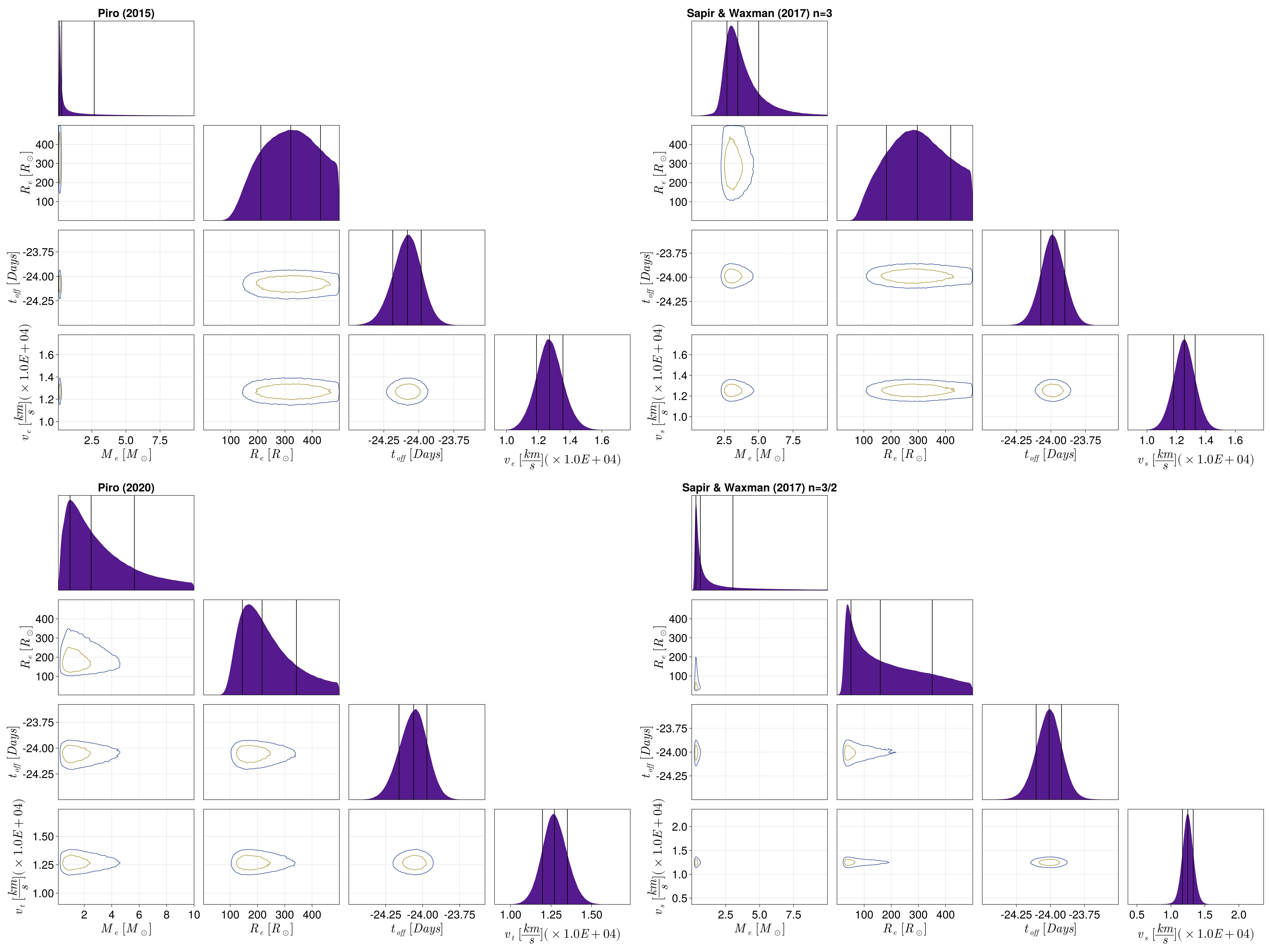
Figure 4: Corner plots of our light curve fit to SN 2021zby. The brown line outlines the $1-\sigma$ joint posterior. The three lines in the individual posterior plots mark the 16th, 50th and 84th percentiles of parameter posteriors, taken as lower-bounds, best fitting values, and upper-bounds. Note that the non-Gaussian posterior may cause biases in determining best fitting values.

Table 1: Priors and results of shock cooling models fit to the shock cooling light curve of SN 2021zby. The upper- and lower-bounds are determined by taking 16th and 84th percentiles of the parameter posteriors. The $M_{e}$ prior was chosen based on physical expectations and is constrained to have a maximum of 10 $M_{\odot}$. Similarly, the prior for $R_{e}$ was chosen based on physical expectations. The $v$ prior was chosen from constraints calculated via a Gaussian fit to He I $10830\AA$ around the shock cooling peak. Finally the constraint on $t$ was chosen from the position of the first TESS observation. The Log-likelihood of each model fit is also listed.

Parameter	Envelope Mass($M_{e}$)	Envelope Radius ($R_{e}$)	Velocity($v$)	Start time ($t$)	Log-likelihood
Prior Function	Levy	Uniform	Normal	Normal	-
PriorInputs	[Location, Scale]	[Min, Max]	[Mean, Std]	[Mean, Std]	-
Input Values	[0, 10]$M_{\odot}$	[0, 500] $R_{\odot}$	[12500, 800]km/s	[-24, 0.5] days	-
SW17 $n=3/2$	$0.638^{+2.396}_{-0.328}M_{\odot}$	$160^{+191}_{-108}R_{\odot}$	$12491^{+798}_{-790}$km/s	$-24.009^{+0.091}_{-0.094}$days	-14.88
SW17 $n=3$	$3.483^{+1.517}_{-0.789}M_{\odot}$	$297^{+123}_{-113}R_{\odot}$	$12542^{+734}_{-728}$km/s	$-23.986^{+0.088}_{-0.086}$ days	-16.26
P15	$0.287^{+2.390}_{-0.158}M_{\odot}$	$321^{+109}_{-110}R_{\odot}$	$12703^{+850}_{-818}$km/s	$-24.081^{+0.099}_{-0.105}$ days	-34.29
P20	$2.503^{+3.146}_{-1.537}M_{\odot}$	$217^{+126}_{-72}R_{\odot}$	$12712^{+793}_{-741}$km/s	$-23.986^{+0.090}_{-0.099}$ days	-23.42

3.1 Fitting light curve with models

There are a number of semi-analytical shock cooling light curve models available, including Piro (2015) (hereafter P15), Piro et al. (2020) (hereafter P20), and Sapir & Waxman (2017) (hereafter SW17). P15 is the simplest of these, making no assumption about the density profile of the progenitor and assuming a simple expanding photosphere. P20 is a revision of the P15 model which improves upon P15 by employing a two-component velocity model. P20 models the progenitor with outer material which has a steep velocity gradient, and inner material with a shallow velocity gradient. SW17 assumes the progenitor has a polytropic density profile. This is characterised by the polytropic index $n$ which is equal to $3/2$ for progenitors with a convective envelope, such as red supergiants (RSG) or yellow supergiant (YSG), and equal to $3$ for progenitors with a radiative envelope, such as blue supergiants (BSG). Each model is parameterised by an envelope mass ($M_{e}$), envelope radius ($R_{e}$), velocity ($v$), and start time ($t$) which is relative to the peak of the radioactive portion of the light curve.

Each of these models assume that the progenitor radiates as a black body and uses an analytical description of the luminosity, radius, and temperature of the progenitor over time in order to derive the flux of the shock cooling light curve. Full details of these analytical models can be found in Armstrong et al. (2021), who we closely follow.

Following Armstrong et al. (2021), we fit the shock cooling models using an affine-invariant MCMC method (ShockCooling.jl: https://github.com/OmegaLambda1998/ShockCooling). This algorithm produces an approximate posterior for a model, given data, priors, and a likelihood function. Our data consists of the ATLAS-$o$ and the 6 hour binned TESS light curve, up to$\sim 7$ days after explosion, the time when the shock cooling light curve transitions into the radioactive light curve. Our likelihood function is chosen to be the reduced $\chi^{2}$ between the models and our data. Both bands are fitted simultaneously, and the combined reduced $\chi^{2}$ is then minimised. The reduced $\chi^{2}$, defined as $\chi^{2}$ divided by the degrees-of-freedom of each band, allows us to weight each reduced $\chi^{2}$ by the number of data points, accounting for the larger sample of TESS data. Due to the degeneracy inherent in the models, the choice of priors has a large effect on the final fit. As such, we used an iterative approach to defining the priors, starting with large uniform priors with $0<R_{e}/R_{\odot}<500$ and $0<M_{e}/M_{\odot}<10$ and then using the posterior to update our choice of prior. The prior of ejecta velocity is constrained to be $12500\pm 800$ km/s, determined by the FWHM of the $1.1~{}\mu$m feature around the shock cooling peak as discussed in the following section. Our final priors for each parameter are listed in Table 1. The best-fit values of SW17 models satisfy the validity range of temperature $T>0.7$eV within the fitting range.

The fitting results for four models discussed are also included in Table 1 and plotted in Figure 3. Figure 4 shows the corner plots of posterior distributions of each parameter. The lower-bound, best-fitted value, and upper-bound are determined by the 16th, 50th, and 84th percentiles in the posterior distributions. Among these models, SW17 $n=3/2$ and $n=3$ models have significantly smaller residuals and larger log-likelihood than P15 and P20 models. Thus, from the light curve fit alone, the SW17 $n=3/2$ models are preferable in general, while the SW17 $n=3$ model performs marginally worse than the $n=3/2$ model. We note that the posteriors of some parameters are highly non-Gaussian, e.g. $R_{e}$ in SW17 $n=3/2$ model, and thus may not accurately represent the best-fit values. For future analyses, we will explore refinements to our SCL-fitting procedure such as using a redefined maximum likelihood estimator, which could possibly improve the P15 and P20 fits.

3.2 Spectroscopic features

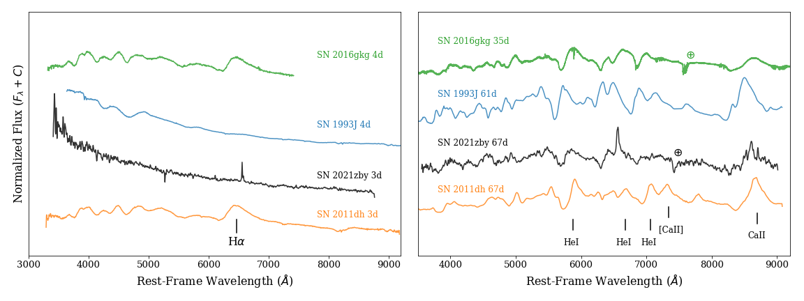
Figure 5: The spectra of SN 2021zby on 3 days (left) and 67 days (right) after explosion, in comparison with SN 2016gkg (Tartaglia et al., 2017), SN 2011dh (Ergon et al., 2015) and SN 1993J (Matheson et al., 2000). All the spectra have been normalized and shifted for clarity.

As shown in Figure 2, the optical spectra around the shock cooling phase are dominated by black body continuum with $T_{BB}\gtrsim 10^{4}$ K with few line features except the narrow H$\alpha$ emission from the host. In Figure 5, we further include the optical spectra from other SNe IIb with SCL around shock cooling phase and late phase. Around the shock cooling peak, there is no detection of broad H$\alpha$ emission in the spectra of SN 2021zby, which is a prominent feature in SN 2011dh and SN 2016gkg at a similar phase (Arcavi et al., 2011; Tartaglia et al., 2017). Benetti et al. (1994) reported the discovery of narrow lines with $v<1000$km/s in SN 1993J around the shock cooling phase, including H$\alpha$, He II, [Fe X] and [Fe XIV], and claimed that those narrow emission lines are signals of circumsteller medium (CSM) interaction. Such features are not seen in the early spectra of SN 2021zby, possibly due to the relatively low S/N and spectral resolution. As shown in Figure 2 and 5, the optical spectra after the shock cooling phase during the radioactive peak start to resemble the spectral evolution of a typical SN IIb.

The weak H$\alpha$ feature of SN 2021zby is persistent and still observable even at 43 days after the radioactive peak. This is different from SN 1993J for which the H$\alpha$ feature significantly weakened at a similar phase (Matheson et al., 2000). This may indicate a sizeable mass of Hydrogen in the progenitor of SN 2021zby.

The NIR spectrum taken by IRTF around the shock cooling peak is plotted in the bottom panel of Figure 2 in comparison with NIR spectra of SN 2016gkg and SN2011dh around similar phase. The only significant feature is the broad emission line at around $10800$Å, which may come from Pa$\gamma$, He I $1.083\mu$m, C I $1.0693\mu$m, or Mg II $1.0927\mu$m as discussed in Shahbandeh et al. (2022). Unlike SN 2011dh and SN 2016gkg, there is no detection of Pa $\beta 1.2818\mu$m feature. On the other hand, a weak emission feature is present around He I $2.0581\mu$m, while there are no detections of Mg II $2.1369\mu$m in the NIR or any other H I or C I features in the optical spectrum at a similar phase. We therefore conclude that this $1.1\mu$m feature most likely comes from He I $1.083\mu$m. We measure the FWHM of this $1.1\mu$m feature with a simple Gaussian fit and use it as the prior of the ejecta velocity in the light curve fitting (see Table 1).

4 Discussion and Conclusion

The progenitor of SN 2021zby is likely to have a moderately extended envelope to produce a clear shock cooling peak, but not as extended as those of SNe IIP progenitors as the peak is not blended with the radioactive peak. With the high-cadence TESS and ATLAS$-o$ light curves covering the full shock cooling phase of SN 2021zby, we are able to constrain the progenitor’s properties with relatively high precision compared to ground-based observations alone. We fit the multi-band light curves following the fitting scheme described in Armstrong et al. (2021), and the best-fit models are:

• The SW17 $n=3/2$ model (convective envelope, i.e. similar to those of RSG or YSG) indicates a progenitor with envelope mass of $\sim 0.3-3.0M_{\odot}$ and envelope radius of $\sim 50-350R_{\odot}$.

• The SW17 $n=3$ model (radiative envelope, i.e. similar to that of BSG) gives the second-best fit with a marginally larger log-likelihood, and indicates an envelope mass of $\sim 2.7-5.0M_{\odot}$ and envelope radius of $\sim 184-420R_{\odot}$. However, such an envelope radius is significantly larger than the expected radii of BSGs, which are in the range of $40-80R_{\odot}$(Underhill et al., 1979). This implies that it is physically inconsistent with observations of the structure of BSGs.

In the previous study on SN 2017jgh, a similar fitting schemes was applied to its Kepler light curve (Armstrong et al., 2021), and they also found that the SW17 $n=3/2$ model is the best-fit model, while the SW17 $n=3$ model performs marginally worse. The best-fit result of SN 2017jgh indicates its progenitor to be most likely a YSG with envelope radius $R_{e}\sim 50-290R_{\odot}$ and envelope mass $M_{e}\lesssim 1.7M_{\odot}$. A few other SNe IIb has progenitors discovered in pre-SN images, enabling another approach to constrain progenitor properties. Aldering et al. (1994) identify the progenitor of SN 1993J as a YSG of type K0 Ia with SED and luminosity, and estimated the radius to be $\sim 500R_{\odot}$. For SN 2016gkg, Kilpatrick et al. (2022) constrained the progenitor to be a YSG as well, with radius $\sim 70R_{\odot}$, which matches $40-150R_{\odot}$ estimate from light curve fit by Arcavi et al. (2017a). For SN 2011dh, Bersten et al. (2012) compared its $g$-light curve with models and also found a YSG with $R\sim 200R_{\odot}$ to be the best match for its progenitor, which is confirmed by the pre- and post-explosion images (Van Dyk et al., 2013). The progenitor radius of SN 2021zby estimated from the best-fit SW17 $n=3/2$ model lies in between these SNe IIb confirmed with YSG progenitors, indicating that SN 2021zby may have a YSG progenitor as well, though the possibility of RSG progenitor cannot be excluded by current light curve fitting alone.

The early spectra of SN 2021zby during SCL shows clear differences compared to the other SNe IIb with similar SCLs. Unlike SN 2011dh and SN 2016gkg, SN 2021zby lacks H features in the shock cooling phase. Such a phenomenon might be a consequence of high ionization around the shock cooling phase (Dessart et al., 2018). This argument is further supported by the blue continuum of the early spectra. On the other hand, the presence of broad He I$10830$ at early times and a relatively strong H$\alpha$ feature after 43 days post-peak indicates that the progenitor still had a sizable amount of H and He.

The high cadences of Kepler and TESS are crucial to sufficiently constrain the progenitor properties with the model fitting of the SCL. However, even with such exquisite data, it is still challenging to fully break the degeneracy between the RSG and YSG progenitors, which could be distinguished either through observations in the UV band, where the signal is most prominent, or by constraining the wind speed with the flash ionized features with high-resolution spectra. With improving cadence and receiving earlier alerts from, for example, Rubin Observatory (Ivezić et al., 2019) in the near future, we can expect to have better time and wavelength coverage in bluer bands. In the longer term, the next generation of MIDEX space-based UV telescopes, e.g. UVEX(Kulkarni et al., 2021) and STAR-X (Saha et al., 2017), will allow us to monitor SCLs in the UV.

Software and third party data repository citations

Table 2: Log of Spectroscopic Observations of SN 2021zby

MJD	Phase relative to $t_{0}$	Phase relative to $t_{peak}$	Telescope/Instrument	Wavelength Range
	[days]	[days]		[Å]
59476.745	2.29	-21.69	SSO 2.3m/WiFeS	3500-9000
59482.491	7.89	-16.09	IRTF/SpeX	6848-25378
59483.466	8.84	-15.14	Shane/KAST	3506-10094
59496.114	21.16	-2.81	LT/SPRAT	4020-7994
59501.265	26.18	2.21	NTT/EFOSC2	3652-9248
59503.594	28.45	4.48	Shane/KAST	3256-10896
59504.653	29.48	5.51	SSO 2.3m/WiFeS	3500-9000
59511.619	36.28	12.30	FTS/FLOYDS	3500-10000
59515.092	39.66	15.68	INT/IDS	3855-8627
59515.300	39.86	15.89	NTT/EFOSC2	3651-9245
59520.520	44.95	20.98	FTN/FLOYDS	3500-10000
59527.470	51.73	27.75	FTN/FLOYDS	3500-10000
59543.206	67.06	43.08	NTT/EFOSC2	3652-9248

References

- Alard & Lupton (1998) Alard, C., & Lupton, R. H. 1998, ApJ, 503, 325, doi: 10.1086/305984
- Aldering et al. (1994) Aldering, G., Humphreys, R. M., & Richmond, M. 1994, AJ, 107, 662, doi: 10.1086/116886
- Andrews et al. (2022) Andrews, J. E., Pearson, J., Lundquist, M. J., et al. 2022, ApJ, 938, 19, doi: 10.3847/1538-4357/ac8ea7
- Arcavi et al. (2011) Arcavi, I., Gal-Yam, A., Yaron, O., et al. 2011, ApJ, 742, L18, doi: 10.1088/2041-8205/742/2/L18
- Arcavi et al. (2017a) Arcavi, I., Hosseinzadeh, G., Brown, P. J., et al. 2017a, ApJ, 837, L2, doi: 10.3847/2041-8213/aa5be1
- Arcavi et al. (2017b) Arcavi, I., Howell, D. A., Kasen, D., et al. 2017b, Nature, 551, 210, doi: 10.1038/nature24030
- Armstrong et al. (2021) Armstrong, P., Tucker, B. E., Rest, A., et al. 2021, MNRAS, 507, 3125, doi: 10.1093/mnras/stab2138
- Arnett & Meakin (2011) Arnett, W. D., & Meakin, C. 2011, ApJ, 741, 33, doi: 10.1088/0004-637X/741/1/33
- Arnett et al. (2018) Arnett, W. D., Hirschi, R., Campbell, S. W., et al. 2018, arXiv e-prints, arXiv:1810.04659. https://arxiv.org/abs/1810.04659
- Astropy Collaboration et al. (2013) Astropy Collaboration, Robitaille, T. P., Tollerud, E. J., et al. 2013, A&A, 558, A33, doi: 10.1051/0004-6361/201322068
- Astropy Collaboration et al. (2018) Astropy Collaboration, Price-Whelan, A. M., Sipőcz, B. M., et al. 2018, AJ, 156, 123, doi: 10.3847/1538-3881/aabc4f
- Becker (2015) Becker, A. 2015, HOTPANTS: High Order Transform of PSF ANd Template Subtraction, Astrophysics Source Code Library, record ascl:1504.004. http://ascl.net/1504.004
- Benetti et al. (1994) Benetti, S., Patat, F., Turatto, M., et al. 1994, A&A, 285, L13
- Bersten et al. (2012) Bersten, M. C., Benvenuto, O. G., Nomoto, K., et al. 2012, ApJ, 757, 31, doi: 10.1088/0004-637X/757/1/31
- Bertin et al. (2002) Bertin, E., Mellier, Y., Radovich, M., et al. 2002, 281, 228. https://ui.adsabs.harvard.edu/abs/2002ASPC..281..228B
- Berton et al. (2018) Berton, M., Congiu, E., Benetti, S., & Yaron, O. 2018, Transient Name Server Classification Report, 2018-1726, 1
- Buzzoni et al. (1984) Buzzoni, B., Delabre, B., Dekker, H., et al. 1984, The Messenger, 38, 9
- Chen et al. (2022) Chen, Z. H., Yan, L., Kangas, T., et al. 2022, arXiv e-prints, arXiv:2202.02060. https://arxiv.org/abs/2202.02060
- Childress et al. (2014) Childress, M. J., Vogt, F. P. A., Nielsen, J., & Sharp, R. G. 2014, Ap&SS, 349, 617, doi: 10.1007/s10509-013-1682-0
- Cushing et al. (2004) Cushing, M. C., Vacca, W. D., & Rayner, J. T. 2004, PASP, 116, 362, doi: 10.1086/382907
- DePoy et al. (2008) DePoy, D., Abbott, T., Annis, J., et al. 2008, in Ground-based and Airborne Instrumentation for Astronomy II, Vol. 7014, International Society for Optics and Photonics, 70140E
- Dessart et al. (2011) Dessart, L., Hillier, D. J., Livne, E., et al. 2011, MNRAS, 414, 2985, doi: 10.1111/j.1365-2966.2011.18598.x
- Dessart et al. (2018) Dessart, L., Yoon, S.-C., Livne, E., & Waldman, R. 2018, A&A, 612, A61, doi: 10.1051/0004-6361/201732363
- Dimitriadis et al. (2019) Dimitriadis, G., Foley, R. J., Rest, A., et al. 2019, ApJ, 870, L1, doi: 10.3847/2041-8213/aaedb0
- Dopita et al. (2007) Dopita, M., Hart, J., McGregor, P., et al. 2007, Ap&SS, 310, 255, doi: 10.1007/s10509-007-9510-z
- Ensman & Woosley (1988) Ensman, L. M., & Woosley, S. E. 1988, ApJ, 333, 754, doi: 10.1086/166785
- Ergon et al. (2015) Ergon, M., Jerkstrand, A., Sollerman, J., et al. 2015, A&A, 580, A142, doi: 10.1051/0004-6361/201424592
- Fang et al. (2022) Fang, Q., Maeda, K., Kuncarayakti, H., et al. 2022, ApJ, 928, 151, doi: 10.3847/1538-4357/ac4f60
- Fausnaugh et al. (2019) Fausnaugh, M., Vallely, P., Kochanek, C., et al. 2019, arXiv preprint arXiv:1904.02171
- Filippenko et al. (1993) Filippenko, A. V., Matheson, T., & Ho, L. C. 1993, ApJ, 415, L103, doi: 10.1086/187043
- Flaugher et al. (2015) Flaugher, B., Diehl, H. T., Honscheid, K., et al. 2015, AJ, 150, 150, doi: 10.1088/0004-6256/150/5/150
- Flewelling et al. (2020) Flewelling, H. A., Magnier, E. A., Chambers, K. C., et al. 2020, ApJS, 251, 7, doi: 10.3847/1538-4365/abb82d
- Folatelli et al. (2014) Folatelli, G., Bersten, M. C., Benvenuto, O. G., et al. 2014, ApJ, 793, L22, doi: 10.1088/2041-8205/793/2/L22
- Foley et al. (2007) Foley, R. J., Smith, N., Ganeshalingam, M., et al. 2007, ApJ, 657, L105, doi: 10.1086/513145
- Fulton et al. (2021) Fulton, M., Smartt, S. J., Sim, S. A., et al. 2021, Transient Name Server Classification Report, 2021-3521, 1
- Gagliano et al. (2018) Gagliano, R., Post, R., Weinberg, E., Newton, J., & Puckett, T. 2018, Transient Name Server Discovery Report, 2018-1685, 1
- Gal-Yam (2017) Gal-Yam, A. 2017, Observational and Physical Classification of Supernovae, ed. A. W. Alsabti & P. Murdin, 195, doi: 10.1007/978-3-319-21846-5_35
- Gilkis & Arcavi (2022) Gilkis, A., & Arcavi, I. 2022, MNRAS, 511, 691, doi: 10.1093/mnras/stac088
- Gilkis et al. (2019) Gilkis, A., Vink, J. S., Eldridge, J. J., & Tout, C. A. 2019, MNRAS, 486, 4451, doi: 10.1093/mnras/stz1134
- Gomez et al. (2021) Gomez, S., Berger, E., Hosseinzadeh, G., et al. 2021, ApJ, 913, 143, doi: 10.3847/1538-4357/abf5e3
- Haas et al. (2010) Haas, M. R., Batalha, N. M., Bryson, S. T., et al. 2010, The Astrophysical Journal Letters, 713, L115
- Harris et al. (2020) Harris, C. R., Millman, K. J., van der Walt, S. J., et al. 2020, Nature, 585, 357–362, doi: 10.1038/s41586-020-2649-2
- Heger et al. (2003) Heger, A., Fryer, C. L., Woosley, S. E., Langer, N., & Hartmann, D. H. 2003, ApJ, 591, 288, doi: 10.1086/375341
- Hinkle (2021) Hinkle, J. 2021, Transient Name Server Classification Report, 2021-3283, 1
- Howell et al. (2014) Howell, S. B., Sobeck, C., Haas, M., et al. 2014, PASP, 126, 398, doi: 10.1086/676406
- Huber et al. (2015) Huber, M., Chambers, K. C., Flewelling, H., et al. 2015, The Astronomer’s Telegram, 7153, 1
- Hunter (2007) Hunter, J. D. 2007, Computing in Science & Engineering, 9, 90, doi: 10.1109/MCSE.2007.55
- Ivezić et al. (2019) Ivezić, Ž., Kahn, S. M., Tyson, J. A., et al. 2019, ApJ, 873, 111, doi: 10.3847/1538-4357/ab042c
- Jacobson-Galán et al. (2022) Jacobson-Galán, W. V., Dessart, L., Jones, D. O., et al. 2022, ApJ, 924, 15, doi: 10.3847/1538-4357/ac3f3a
- Kilpatrick et al. (2022) Kilpatrick, C. D., Coulter, D. A., Foley, R. J., et al. 2022, ApJ, 936, 111, doi: 10.3847/1538-4357/ac8a4c
- Kulkarni et al. (2021) Kulkarni, S. R., Harrison, F. A., Grefenstette, B. W., et al. 2021, arXiv e-prints, arXiv:2111.15608. https://arxiv.org/abs/2111.15608
- Lohev et al. (2019) Lohev, N., Sabach, E., Gilkis, A., & Soker, N. 2019, MNRAS, 490, 9, doi: 10.1093/mnras/stz2593
- Long et al. (2022) Long, G., Song, H.-F., Zhang, R.-Y., et al. 2022, Research in Astronomy and Astrophysics, 22, 055016, doi: 10.1088/1674-4527/ac60d3
- Matheson et al. (2000) Matheson, T., Filippenko, A. V., Barth, A. J., et al. 2000, AJ, 120, 1487, doi: 10.1086/301518
- Maund et al. (2004) Maund, J. R., Smartt, S. J., Kudritzki, R. P., Podsiadlowski, P., & Gilmore, G. F. 2004, Nature, 427, 129, doi: 10.1038/nature02161
- Maund et al. (2011) Maund, J. R., Fraser, M., Ergon, M., et al. 2011, ApJ, 739, L37, doi: 10.1088/2041-8205/739/2/L37
- Pearson et al. (2022) Pearson, J., Hosseinzadeh, G., Sand, D. J., et al. 2022, arXiv e-prints, arXiv:2208.14455. https://arxiv.org/abs/2208.14455
- Piascik et al. (2014) Piascik, A. S., Steele, I. A., Bates, S. D., et al. 2014, in Society of Photo-Optical Instrumentation Engineers (SPIE) Conference Series, Vol. 9147, Ground-based and Airborne Instrumentation for Astronomy V, ed. S. K. Ramsay, I. S. McLean, & H. Takami, 91478H, doi: 10.1117/12.2055117
- Piro (2015) Piro, A. L. 2015, ApJ, 808, L51, doi: 10.1088/2041-8205/808/2/L51
- Piro et al. (2020) Piro, A. L., Haynie, A., & Yao, Y. 2020, arXiv e-prints, arXiv:2007.08543. https://arxiv.org/abs/2007.08543
- Rayner et al. (2003) Rayner, J. T., Toomey, D. W., Onaka, P. M., et al. 2003, PASP, 115, 362, doi: 10.1086/367745
- Rest et al. (2005) Rest, A., Stubbs, C., Becker, A. C., et al. 2005, The Astrophysical Journal, 634, 1103, doi: 10.1086/497060
- Rest et al. (2013) Rest, A., Scolnic, D., Foley, R. J., et al. 2013, doi: 10.1088/0004-637X/795/1/44
- Ricker et al. (2014) Ricker, G. R., Winn, J. N., Vanderspek, R., et al. 2014, in Society of Photo-Optical Instrumentation Engineers (SPIE) Conference Series, Vol. 9143, Space Telescopes and Instrumentation 2014: Optical, Infrared, and Millimeter Wave, ed. J. Oschmann, Jacobus M., M. Clampin, G. G. Fazio, & H. A. MacEwen, 914320, doi: 10.1117/12.2063489
- Ridden-Harper et al. (2021) Ridden-Harper, R., Rest, A., Hounsell, R., et al. 2021, arXiv e-prints, arXiv:2111.15006. https://arxiv.org/abs/2111.15006
- Riess et al. (2016) Riess, A. G., Macri, L. M., Hoffmann, S. L., et al. 2016, ApJ, 826, 56, doi: 10.3847/0004-637X/826/1/56
- Riess et al. (2018) Riess, A. G., Casertano, S., Yuan, W., et al. 2018, ApJ, 861, 126, doi: 10.3847/1538-4357/aac82e
- Saha et al. (2017) Saha, T. T., Zhang, W. W., & McClelland, R. S. 2017, in Society of Photo-Optical Instrumentation Engineers (SPIE) Conference Series, Vol. 10399, Society of Photo-Optical Instrumentation Engineers (SPIE) Conference Series, 103990I, doi: 10.1117/12.2273803
- Sana et al. (2012) Sana, H., de Mink, S. E., de Koter, A., et al. 2012, Science, 337, 444, doi: 10.1126/science.1223344
- Sapir & Waxman (2017) Sapir, N., & Waxman, E. 2017, ApJ, 838, 130, doi: 10.3847/1538-4357/aa64df
- Schechter et al. (1993) Schechter, P. L., Mateo, M., & Saha, A. 1993, Publications of the Astronomical Society of the Pacific, 105, 1342, doi: 10.1086/133316
- Schlafly & Finkbeiner (2011) Schlafly, E. F., & Finkbeiner, D. P. 2011, ApJ, 737, 103, doi: 10.1088/0004-637X/737/2/103
- Scolnic et al. (2015) Scolnic, D., Casertano, S., Riess, A., et al. 2015, ApJ, 815, 117, doi: 10.1088/0004-637X/815/2/117
- Shahbandeh et al. (2022) Shahbandeh, M., Hsiao, E. Y., Ashall, C., et al. 2022, ApJ, 925, 175, doi: 10.3847/1538-4357/ac4030
- Smartt et al. (2015) Smartt, S. J., Valenti, S., Fraser, M., et al. 2015, A&A, 579, A40, doi: 10.1051/0004-6361/201425237
- Smith et al. (2020) Smith, K. W., Smartt, S. J., Young, D. R., et al. 2020, PASP, 132, 085002, doi: 10.1088/1538-3873/ab936e
- Smith et al. (2021) Smith, K. W., Srivastav, S., Smartt, S. J., et al. 2021, Transient Name Server AstroNote, 246, 1
- Smith (2017) Smith, N. 2017, Interacting Supernovae: Types IIn and Ibn, ed. A. W. Alsabti & P. Murdin, 403, doi: 10.1007/978-3-319-21846-5_38
- Soker (2017) Soker, N. 2017, MNRAS, 470, L102, doi: 10.1093/mnrasl/slx089
- Springob et al. (2005) Springob, C. M., Haynes, M. P., Giovanelli, R., & Kent, B. R. 2005, ApJS, 160, 149, doi: 10.1086/431550
- Sravan et al. (2020) Sravan, N., Marchant, P., Kalogera, V., Milisavljevic, D., & Margutti, R. 2020, ApJ, 903, 70, doi: 10.3847/1538-4357/abb8d5
- STScI Development Team (2013) STScI Development Team. 2013, pysynphot: Synthetic photometry software package. http://ascl.net/1303.023
- Tartaglia et al. (2017) Tartaglia, L., Fraser, M., Sand, D. J., et al. 2017, ApJ, 836, L12, doi: 10.3847/2041-8213/aa5c7f
- Tody (1986) Tody, D. 1986, in Society of Photo-Optical Instrumentation Engineers (SPIE) Conference Series, Vol. 627, Instrumentation in astronomy VI, ed. D. L. Crawford, 733, doi: 10.1117/12.968154
- Tonry et al. (2018) Tonry, J., Denneau, L., Heinze, A., et al. 2018, Publications of the Astronomical Society of the Pacific, 130, 064505
- Underhill et al. (1979) Underhill, A. B., Divan, L., Prevot-Burnichon, M. L., & Doazan, V. 1979, MNRAS, 189, 601, doi: 10.1093/mnras/189.3.601
- Vacca et al. (2003) Vacca, W. D., Cushing, M. C., & Rayner, J. T. 2003, PASP, 115, 389, doi: 10.1086/346193
- Valdes et al. (2014) Valdes, F., Gruendl, R., & DES Project. 2014, 485, 379. https://ui.adsabs.harvard.edu/abs/2014ASPC..485..379V
- Valenti et al. (2013) Valenti, S., Sand, D., Pastorello, A., et al. 2013, Monthly Notices of the Royal Astronomical Society: Letters, 438, L101, doi: 10.1093/mnrasl/slt171
- Vallely et al. (2019) Vallely, P. J., Fausnaugh, M., Jha, S. W., et al. 2019, MNRAS, 487, 2372, doi: 10.1093/mnras/stz1445
- Van Dyk et al. (2013) Van Dyk, S. D., Zheng, W., Clubb, K. I., et al. 2013, ApJ, 772, L32, doi: 10.1088/2041-8205/772/2/L32
- Van Dyk et al. (2014) Van Dyk, S. D., Zheng, W., Fox, O. D., et al. 2014, AJ, 147, 37, doi: 10.1088/0004-6256/147/2/37
- Virtanen et al. (2020) Virtanen, P., Gommers, R., Oliphant, T. E., et al. 2020, Nature Methods, 17, 261, doi: 10.1038/s41592-019-0686-2
- Wang et al. (2021) Wang, Q., Rest, A., Zenati, Y., et al. 2021, ApJ, 923, 167, doi: 10.3847/1538-4357/ac2c84
- Woosley et al. (1993) Woosley, S. E., Langer, N., & Weaver, T. A. 1993, ApJ, 411, 823, doi: 10.1086/172886
- Yaron & Gal-Yam (2012) Yaron, O., & Gal-Yam, A. 2012, PASP, 124, 668, doi: 10.1086/666656
- Yoon et al. (2017) Yoon, S.-C., Dessart, L., & Clocchiatti, A. 2017, ApJ, 840, 10, doi: 10.3847/1538-4357/aa6afe
- Zenati et al. (2022) Zenati, Y., Wang, Q., Bobrick, A., et al. 2022, arXiv e-prints, arXiv:2207.07146. https://arxiv.org/abs/2207.07146