Non-equilibrium relaxations:
ageing and finite-size effects

Malte Henkel^a,b

^aLaboratoire de Physique et Chimie Théoriques (CNRS UMR 7019),

Université de Lorraine Nancy, B.P. 70239, F – 54506 Vandœuvre lès Nancy Cedex, France

^bCentro de Física Teórica e Computacional, Universidade de Lisboa,

Campo Grande, P–1749-016 Lisboa, Portugal

The long-time behaviour of spin-spin correlators in the slow relaxation of systems undergoing phase-ordering kinetics is studied in geometries of finite size. A phenomenological finite-size scaling ansatz is formulated and tested through the exact solution of the kinetic spherical model, quenched to below the critical temperature, in $2<d<4$ dimensions.  
 

PACS numbers: 05.40.-a, 05.70.Ln, 05.70.Jk, 75.40.Gb

1 Critical relaxations in finite-size systems

Collective phenomena arise in many-body systems with dynamically created long-range interactions and thereby often show new qualitative properties which cannot be obtained in systems with a small number of degrees of freedom. An important class are critical phenomena, characterised by scale-invariance. We are interested here in time-dependent phenomena with time-dependent or ‘dynamical’ scaling. As a physical example, we consider many-body spin systems, initially prepared in a disordered state with at most short-ranged correlations and then suddenly quenched to a temperature $0<T<T_{c}$ below the critical temperature $T_{c}>0$, with at least two physically distinct phases. Such a quenched spin system is then said to undergo phase-ordering kinetics [17]. For a spatially infinite geometry, observables such as correlation functions are then expected to be invariant under the time-space dilatation

$$t\mapsto t^{\prime}=\kappa^{z}t\;\;,\;\;\boldsymbol{r}\mapsto\boldsymbol{r}^{\prime}=\kappa\boldsymbol{r}$$ (1.1)

where $\kappa$ is a constant re-scaling factor and the dynamical exponent $z$ serves to distinguish the scaling between time and space. The relaxation of the system after the quench can be measured through connected correlators of the time- and space-dependent spin variables $S_{\boldsymbol{r}}(t)$, namely

$$C(t;\boldsymbol{r}) :=\left\langle S_{\boldsymbol{r}}(t)S_{\boldsymbol{0}}(t)\right\rangle-\left\langle S_{\boldsymbol{r}}(t)\right\rangle\left\langle S_{\boldsymbol{0}}(t)\right\rangle=F_{C}\left(\frac{|\boldsymbol{r}|}{t^{1/z}}\right)$$ (1.2a)

$$C(t,s) :=\left\langle S_{\boldsymbol{r}}(t)S_{\boldsymbol{r}}(s)\right\rangle-\left\langle S_{\boldsymbol{r}}(t)\right\rangle\left\langle S_{\boldsymbol{r}}(s)\right\rangle=f_{C}\left(\frac{t}{s}\right)$$ (1.2b)

where the quoted scaling forms are meant to hold in the limit of large times and large distances, such that $|\boldsymbol{r}|^{z}/t$ and $t/s$ are kept fixed. In (1.2b), $t$ is the observation time and $s$ is the waiting time. Asymptotically, the scaling function $f_{C}(y)$ in (1.2b) should be algebraic

$$f_{C}(y)\sim y^{-\lambda/z}\;\;,\;\;\mbox{\rm as $y\to\infty$}$$ (1.3)

where $\lambda=\lambda_{C}$ is the autocorrelation exponent. A many-body non-stationary system whose slow relaxation dynamics also breaks time-translation-invariance and is such that the single-time correlator $C(t,\boldsymbol{r})$ and the two-time auto-correlator $C(t,s)$ obey the dynamical scaling (1.2), is said to be ageing [71, 32, 49, 73].

material/model			$\,z$	$\lambda$	Refs.
Merck (CCH-501)			$1.94(5)$	$1.246(79)$	[61]
nematic TNLC			$2.01(1)$	$1.28(11)$	[5]
Ising	$1D$	lr	$1+\sigma$	$0.5$	[28, 29]
Ising	$2D$	lr	$1+\sigma$	$1$	[24, 25]
Ising	$2D$	sr	2	$1.24(2)$	[56]
			2	$1.25$	[24, 25]
			2	$1.3$	[62, 63, 74]
Ising	$3D$	sr	$2$	$1.60(2)$	[48]
			$2$	$1.6$	[62, 63]
Potts-3	$2D$	sr	$2$	$1.19(3)$	[56]
			$2$	$1.22(2)$	[27]
Potts-8	$2D$	sr	$2$	$1.25(1)$	[56]
$XY$	$3D$	sr	$2$	$1.7(1)$	[2]
			$2$	$1.6$	[62]
spherical		sr	$2$	$d/2$	[45]
spherical		lr	$\sigma$	$d/2$	[20, 11]

Table 1: Dynamical exponent $z$ and autocorrelation exponent $\lambda$, as measured experimentally or found in some spin models. Long-range (lr) behaviour occurs in the Ising model for $\sigma<1$ and in the spherical model for $\sigma<2$. The spherical model is considered for dimensions $d>z$.

For phase-ordering, with a non-conserved order parameter, some general exact results exist for models with short-ranged interactions. First, the dynamical exponent $z=2$ for a non-conserved order parameter [18]. Second, the Yeung-Rao-Desai inequality states that $\lambda\geq d/2$ [76]. Third, for the $2D$ Ising model one has the Fisher-Huse inequality $\lambda\leq\frac{5}{4}$ [39]. Some typical values for $z$ and $\lambda$ are listed in table 1. They illustrate the sharpness of these exact bounds and permit a comparison between short-ranged and long-ranged interactions. The agreement with the available experiments [61, 5] is very satisfying. For more detailed tables, see [49].

How is the scaling behaviour, encoded in the scaling forms (1.2), modified in a system confined to a domain of finite size, e.g. because it is placed into a box ?

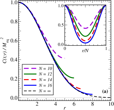
Figure 1: (a) Finite-size effects for the single-time correlator $C(t,\boldsymbol{r})$ in the fully finite spherical model at $T<T_{c}$, with $t=50$ and $N=[10,12,14,16,\infty]$ from top to bottom. The inset shows the periodicity over the interval $0\leq r/N\leq 1$.
(b) Finite-size effects for the two-time autocorrelator $C(ys,s)$ in the $3D$ fully finite spherical model at $T<T_{c}$, for $N=[15,20,30,40]$ from top to bottom (at the right) and $s$ fixed. The thin dashed line gives the infinite-size autocorrelator. The inset shows the data collapse of the re-scaled correlator $CN^{3/2}$ for $y=t/s$ large, with $N=[15,20,25,30,35,40]$ from left to right (arbitrary units).

For a phenomenological answer, consider figure 1. For a fully finite hyper-cubic lattice with $N^{d}$ sites and periodic boundary conditions, the single-time correlator $C(t;\boldsymbol{r})$ is shown in figure 1a, where $\boldsymbol{r}$ is oriented along one of coordinate axes. If the spatial distances $r=|\boldsymbol{r}|$ are not too large, the shape of the correlator does not depend sensitively on $N$. Only if $r\lesssim\frac{N}{2}$, does the correlator also receive contributions ‘from around the world’, such that for $r\approx\frac{N}{2}$ it no longer tends towards zero, but rather saturates at a $N$-dependent constant $C^{(1)}_{\rm lim}(N)>0$. Figure 1b shows the two-time autocorrelator $C(ys,s)$. For large $s$, but $y$ small enough, there is a clear data collapse. However, for larger values of $y$, $C$ begins to decrease more rapidly than the infinite-size curve (1.2b). As $y\gg 1$, $C$ finally saturates at the limit value $C^{(2)}_{\infty}(N)>0$.

Figure 2: Finite-size effects for the longitudinal characteristic length $L_{\|}^{2}(t)$, measured along a coordinate axis, in the fully finite spherical model with lattice sizes $N=[25,50,100,200]$ from bottom to top. The thin dashed line indicates the infinite-size behaviour $L(t)\sim t^{1/2}$.

Although the single-time correlator does not display strong finite-size effects, this is different for the length scale $L=L(t)$ of the growing clusters, estimated from the second moment

$$L^{2}(t)=\frac{\sum_{\boldsymbol{r}}|\boldsymbol{r}|^{2}C(t;\boldsymbol{r})}{\sum_{\boldsymbol{r}}C(t;\boldsymbol{r})}$$ (1.4)

The precise extent of the sums will be specified below. Figure 2 shows that for sufficiently short times, the length $L^{2}(t)\sim t$ behaves as for the infinite system, but as $t$ grows further, finally there occurs a cross-over towards a finite constant $L_{\infty}(N)$. We shall see how to explain the findings of figures 1 and 2 in terms of phenomenological finite-size scaling. The resulting predictions will be tested in the exactly solved kinetic spherical model, for dimensions $2<d<4$.

The spherical model of a ferromagnet [13, 55] has served as an exactly solvable, yet non-trivial, model for the detailed analysis of general concepts of critical phenomena, see [40] for a historical perspective. Its non-equilibrium behaviour after a quench has also been thoroughly analysed, see [67, 30, 31, 45, 20, 43, 64, 47, 6, 11, 34, 7, 49]. The related Arcetri model provides a qualitative description of the dynamics in the non-equilibrium growth of interfaces [50, 33]. Finite-size effects at equilibrium have also been analysed at great depth in the spherical model and have been of value to test the theory of finite-size scaling derived from the renormalisation group, see [8, 19, 9, 57, 69, 70, 65, 4, 16, 22] and refs. therein. For dimensions $d>d_{c}=4$, that is above the upper critical dimension, the standard finite-size scaling ansatz must be considerably modified [14, 65, 51, 41, 42, 46, 12].

Finite-size scaling techniques have been applied in studies of phase-ordering kinetics [63, 74], the ageing of polymer collapse [58, 23, 59, 60] or the dynamics of mitochondrial networks [77]. Explicit studies of finite-size scaling in an ageing system have been carried out in Ising spin glasses [52] and notably on the dimensional cross-over between the $3D$ and $2D$ Edwards-Anderson spin glass [37] as motivated by extremely accurate experiments on CuMn films [78, 79]. In addition, finite-size effects analogous to figures 1 and 2 are clearly visible in the time-evolution of characteristic cluster sizes in long-ranged Ising models quenched to $T<T_{c}$ [24] or in the auto-correlator [25]. Since the bulk $3D$ spherical model and the bulk $(p=2)$ spherical spherical spin glass are in the same dynamic universality class [31], one might hope that finite-size effects could be similar as well. Not so ! Rather, detailed studies of the $(p=2)$ spherical spin glass [44, 10] show that this equivalence only holds in the spin glass for times $t\ll t_{\rm cross}\sim N^{2/3}$. For time scales $t\gg t_{\rm cross}$, ageing still holds with a new set of universal exponents [44], to be followed by a second cross-over to a regime of exponential decay at extremely large times [10].

This work is organised as follows. In section 2, we recall the main features of dynamical scaling in ageing phase-ordering kinetics. In section 3, we extend this phenomenological treatment to finite systems, using the hyper-cubic geometry $\overbrace{N\times\cdots\times N\,}^{d^{*}\>\mbox{\rm\scriptsize factors}}\times\overbrace{\infty\times\cdots\times\infty}^{d-d^{*}\>\mbox{\rm\scriptsize factors}}$, where the first $d^{*}\leq d$ directions are finite and periodic and the other $d-d^{*}$ directions are infinite. The finite-size forms so obtained will be checked in section 4 using the exact solution of the kinetic spherical model in $2<d<4$ dimensions, quenched to $T>T_{c}$ from a totally disordered state and in section 5 we conclude. Technical details of the exact solution are given in the appendix.

2 Dynamical scaling description

A central ingredient of ageing is dynamical scaling. For the general two-time and spatial bulk correlator, our starting point is (below the upper critical dimension $d<d_{c}$; for short-ranged interactions usually $d_{c}^{({\rm short})}=4$)

$$C\left(\kappa^{z}t,\kappa^{z}s;\kappa\boldsymbol{r}\right)=\kappa^{\phi}C\left(t,s;\boldsymbol{r}\right)$$ (2.1)

where $t,s$ are the observation and the waiting time, $z$ is the dynamical exponent, $\phi$ a scaling exponent and $\boldsymbol{r}$ is the spatial distance. Writing (2.1) means that we assume negligible all finite-time and finite-distance corrections to scaling. Choosing $\kappa=s^{-1/z}$, this gives

$$C\left(t,s;\boldsymbol{r}\right)=s^{\phi/z}C\left(\frac{t}{s},1;\frac{\boldsymbol{r}}{s^{1/z}}\right)$$ (2.2)

In phase-ordering, the single-time correlator at $\boldsymbol{r}=\boldsymbol{0}$ is finite; namely either $C(t;\boldsymbol{0})=1$ in Ising-like systems or else $C(t;\boldsymbol{0})=M_{\rm eq}^{2}$ for order parameters with a continuous global symmetry. Setting $s=t$ in (2.2), this leads to $\phi=0$ and further to $C(t;\boldsymbol{r})=C\bigl{(}1,1;|\boldsymbol{r}|t^{-/z}\bigr{)}=:F_{C}(|\boldsymbol{r}|t^{-/z}\bigr{)}$. On the other hand, setting now $\boldsymbol{r}=\boldsymbol{0}$, the two-time auto-correlator is $C(t,s)=C\bigl{(}t,s;\boldsymbol{0}\bigr{)}=C(t/s,1;\boldsymbol{0})=:f_{C}(t/s)$. These results fully reproduce (1.2).

3 Dynamical finite-size scaling

According to the original definition, finite-size scaling [38] is the scaling behaviour in a nearly critical system confined to a geometry of finite linear extent  $N$. For finite geometries, the natural generalisation of (2.1) consists, as at equilibrium [8, 72, 9, 65], to consider $1/N$ as a further relevant scaling field. While this hypothesis was originally specified for the order parameter at the critical point [72], we adapt this to the situation at hand and write down the finite-size scaling (fss) ansatz for the full two-time correlator

$$C\left(\kappa^{z}t,\kappa^{z}s;\kappa\boldsymbol{r};\kappa^{-1}\frac{1}{N}\right)=\kappa^{\phi}C\left(t,s;\boldsymbol{r};\frac{1}{N}\right)$$ (3.1)

meant to hold in the hyper-cubic geometry $\overbrace{N\times\cdots\times N\,}^{d^{*}\>\mbox{\rm\scriptsize factors}}\times\overbrace{\infty\times\cdots\times\infty}^{d-d^{*}\>\mbox{\rm\scriptsize factors}}$ where $N$ describes the finite length in the system. For simplicity, we consider a single length of this kind. Of course, for $N\to\infty$, one is back to the bulk scaling form (2.1), and hence (1.2).

Choose the re-scaling factor $\kappa=s^{-1/z}$. For phase-ordering kinetics, recall from section 2 that $\phi=0$. Then (3.1) can be equivalently expressed as

$$C\left(t,s;\boldsymbol{r};\frac{1}{N}\right)=C\left(\frac{t}{s},1;\frac{\boldsymbol{r}}{s^{1/z}};\frac{s^{1/z}}{N}\right)$$ (3.2)

As above in section 2, we then expect for the correlators (provided spatial rotation-invariance can be assumed)

$$C\bigl{(}t;\boldsymbol{r};N^{-1}\bigr{)}=F_{C}\left(\frac{|\boldsymbol{r}|^{z}}{t};\frac{N^{z}}{t}\right)\;\;,\;\;C\bigl{(}t,s;N^{-1}\bigr{)}=f_{C}\left(\frac{t}{s};\frac{N^{z}}{t}\right)$$ (3.3)

such that the corresponding scaling functions are now functions of two variables. Finite-size scaling in ageing can be analysed in the asymptotic fss limit where $t\to\infty$, $s\to\infty$, $|\boldsymbol{r}|\to\infty$ and $N\to\infty$ such that the three scaling variables

$$y=\frac{t}{s}\;\;~{},~{}\;\;\boldsymbol{\varrho}=\frac{\boldsymbol{r}}{t^{1/z}}\;\;~{},~{}\;\;Z=\frac{N^{z}}{t}$$ (3.4)

are kept fixed. The precise form of the finite-size scaling functions (3.3) will depend on the universality class under study, and on the boundary conditions [9, 65, 16].

As a first consequence, consider the characteristic length $L(t)$ of the clusters. From (1.4) and (3.3), we derive the finite-size scaling form

$$L^{2}(t;N^{-1})=\frac{\sum_{\boldsymbol{r}}|\boldsymbol{r}|^{2}C(t;\boldsymbol{r};N^{-1})}{\sum_{\boldsymbol{r}}C(t;\boldsymbol{r};N^{-1})}\simeq t^{2/z}\frac{\int\!{\rm d}\boldsymbol{r}\>\bigl{(}|\boldsymbol{r}|t^{-1/z}\bigr{)}^{2}F_{C}(|\boldsymbol{r}|^{z}/t;N^{z}/t)}{\int\!{\rm d}\boldsymbol{r}\>F_{C}(|\boldsymbol{r}|^{z}/t;N^{z}/t)}=t^{2/z}f_{L}\left(\frac{N^{z}}{t}\right)$$ (3.5)

For $Z\gg 1$, the behaviour of an effectively infinite system requires that $f_{L}(Z)\stackrel{{\scriptstyle Z\gg 1}}{{\simeq}}f_{0}=\mbox{\rm cste.}$ and for $Z\ll 1$, the time-independent saturation in figure 2 is captured by $f_{L}(Z)\stackrel{{\scriptstyle Z\ll 1}}{{\sim}}Z^{2/z}$ such that $L_{\infty}(N)\sim N$, as would have been expected from dimensional analysis.

Next, we consider the plateau in the two-time auto-correlator $C(ys,s)$ for $y\gg 1$, see figure 1b. Recall that for the infinite system, we expect from (1.2b,1.3) that $C(t,s;\boldsymbol{0};0)=f_{C}(t/s)\sim\bigl{(}t/s\bigr{)}^{-\lambda/z}$. For $N<\infty$, we reformulate (3.2) as follows

$$C\bigl{(}t,s;N^{-1}\bigr{)}=C\left(t,s;\boldsymbol{0};\frac{1}{N}\right)=C\left(\frac{t}{s},1;\boldsymbol{0};\frac{s^{1/z}}{N}\right)=\left(\frac{t}{s}\right)^{-\lambda/z}\mathscr{F}_{C}\left(\left(\frac{t}{s}\right)^{1/z},\frac{s^{1/z}}{N}\right)$$ (3.6)

Herein, the first argument in the scaling function $\mathscr{F}_{C}=\mathscr{F}_{C}\bigl{(}y,u\bigr{)}$ will be considered large and be kept fixed, $y\gg 1$. In that case, the scaling function will describe the cross-over between (i) the infinite-system behaviour (when $u=s^{1/z}/N\to 0$) $f_{C}(y)=\mathscr{F}_{C}(y,0)\sim y^{-\lambda/z}$ which is independent of $s$ and (ii) the fully finite-system behaviour (when $u=s^{1/z}/N\to\infty$) when $C\stackrel{{\scriptstyle y\gg 1}}{{\longrightarrow}}C^{(2)}_{\infty}$ no longer depends on $y=t/s$. The first limit case is taken into account by admitting $\mathscr{F}_{C}(y,u)\simeq\mathtt{F}\bigl{(}yu\bigr{)}$ and $\mathtt{F}(0)=\mbox{\rm cste}$. Then the second limit case leads to

$$C\left(t,s;\boldsymbol{0};\frac{1}{N}\right)\stackrel{{\scriptstyle t/s\gg 1}}{{\simeq}}\left(\frac{t}{s}\right)^{-\lambda/z}\mathtt{F}\left(\left(\frac{t}{s}\right)^{1/z}\cdot\frac{s^{1/z}}{N}\right)\sim\left(\frac{t}{s}\right)^{-\lambda/z}\left(\left(\frac{t}{s}\right)^{1/z}\cdot\frac{s^{1/z}}{N}\right)^{\omega}$$ (3.7)

where in the last step, we assumed a power-law form of $\mathtt{F}(yu)\sim\bigl{(}yu\bigr{)}^{\omega}$ for $yu\gg 1$. The $y$-independent plateau $C^{(2)}_{\infty}$ observed for fully finite systems (see figure 1b for $s$ fixed) is reproduced if we choose $\omega=\lambda$. Hence, for finite systems with $y=t/s\gg 1$

$$C\left(t,s;\boldsymbol{0};\frac{1}{N}\right)\stackrel{{\scriptstyle t/s\gg 1}}{{\longrightarrow}}C^{(2)}_{\infty}\sim\left(\frac{s^{1/z}}{N}\right)^{\lambda}$$ (3.8)

Herein, $s$ is still kept fixed whereas $N$ must be taken large enough such that the system under study is indeed in its finite-size scaling regime (in other word, $Ns^{-1/z}$ must be large enough).

Hence for fully finite systems, quenched to $T<T_{c}$, the auto-correlator $C(ys,s)=f_{C}(y)\stackrel{{\scriptstyle y\gg 1}}{{\longrightarrow}}C^{(2)}_{\infty}$, such that the plateau value $C^{(2)}_{\infty}=C^{(2)}_{\infty}(s,N)$ should obey the scalings

$$C^{(2)}_{\infty}\sim N^{-\lambda}\mbox{\rm~{}~{}with $s$ fixed}\;\;~{}~{},~{}~{}\;\;C^{(2)}_{\infty}\sim s^{\lambda/z}\mbox{\rm~{}~{} with $N$ fixed}$$ (3.9)

These are the sought scalings for the plateau of the autocorrelator and the main result of this section.

The inset in figure 1b shows the data collapse of $N^{\lambda}C(ys,s)$ to a $y$-independent constant for $y$ large enough and $s$ fixed, in the $3D$ spherical model, where $\lambda=\frac{3}{2}$. In the next section, (3.9) will be verified analytically from the exact solution of the quenched kinetic spherical model in dimensions $2<d<4$.

A simple heuristic argument to establish (3.8) goes as follows. For widely different times $t\gg s\gg\tau_{\rm mic}$, the asymptotic form of the autocorrelator is expressed through the cluster sizes $L$ as $C(t,s)\sim\bigl{(}L(t)/L(s)\bigr{)}^{-\lambda}$. If furthermore $t$ is so large that $L(t)\sim N$ while $s$ is small enough such that still $L(s)\sim s^{1/z}$, the scaling (3.8) of the plateau $C_{\infty}^{(2)}$ follows.

4 The kinetic spherical model

Following standard developments [67, 30, 45, 50], the kinetic spherical model is defined in terms of real spin variables $S_{\boldsymbol{n}}=S_{\boldsymbol{n}}(t)\in\mathbb{R}$ at each lattice site $\boldsymbol{n}\in\Lambda\subset\mathbb{Z}^{d}$, subject to the spherical constraint $\sum_{\boldsymbol{n}\in\Lambda}S_{n}^{2}(t)=|\Lambda|$, where $|\Lambda|=\prod_{j=1}^{d}N_{j}$ is the number of sites of the lattice $\Lambda\subset\mathbb{Z}^{d}$. Its dynamics is given by the Langevin equation

$$\partial_{t}S_{\boldsymbol{n}}(t)=D\Delta_{\boldsymbol{n}}S_{\boldsymbol{n}}(t)-\mathfrak{z}(t)S_{\boldsymbol{n}}(t)+\eta_{\boldsymbol{n}}(t)$$ (4.1)

with the spatial laplacian $\Delta_{\boldsymbol{n}}$ and the thermal white noise $\eta_{\boldsymbol{n}}=\eta_{\boldsymbol{n}}(t)$. It has the first two moments

$$\bigl{\langle}\eta_{\boldsymbol{n}}(t)\bigr{\rangle}=0\;\;,\;\;\bigl{\langle}\eta_{\boldsymbol{n}}(t)\eta_{\boldsymbol{m}}(t^{\prime})\bigr{\rangle}=2DT\delta(t-t^{\prime})\delta_{\boldsymbol{n},\boldsymbol{m}}$$ (4.2)

where $T$ is the bath temperature and $D$ a kinetic coefficient. The Lagrange multiplier $\mathfrak{z}(t)$ is fixed from the spherical constraint. The Fourier representation

$$S_{\boldsymbol{n}}(t)=\frac{1}{|\Lambda|}\sum_{k_{1}=0}^{N_{1}-1}\cdots\sum_{k_{d}=0}^{N_{d}-1}\exp\left(2\pi{\rm i}\sum_{j=1}^{d}\frac{k_{j}}{N_{j}}n_{j}\right)\widehat{S}(t,\boldsymbol{k})$$ (4.3)

achieves the formal solution of the model which reads

$$\widehat{S}(t,\boldsymbol{k})=\widehat{S}(0,\boldsymbol{k})\frac{\exp\bigl{(}-2D\omega(\boldsymbol{k})t\bigr{)}}{\sqrt{g(t)\,}}+\int_{0}^{t}\!{\rm d}\tau\>\widehat{\eta}(\tau,\boldsymbol{k})\sqrt{\frac{g(\tau)}{g(t)}\,}\,\exp\bigl{(}-2D\omega(\boldsymbol{k})(t-\tau)\bigr{)}$$ (4.4a)

with the abbreviations (nearest-neighbour interactions assumed)

$$\omega(\boldsymbol{k})=\sum_{j=1}^{d}\left(1-\cos\frac{2\pi}{N_{j}}k_{j}\right)\;\;,\;\;g(t)=\exp\left(2\int_{0}^{t}\!{\rm d}\tau\>\mathfrak{z}(\tau)\right)$$ (4.4b)

In what follows, we restrict to a totally disordered initial state, such that $$\bigl{\langle}S_{\boldsymbol{n}}(0)\bigr{\rangle}=0 \bigl{\langle}S_{\boldsymbol{n}}(0)S_{\boldsymbol{m}}(0)\bigr{\rangle}=\delta_{\boldsymbol{n},\boldsymbol{m}}$$ and . In momentum space, the second moments of initial and thermal noises become

$$\left\langle\widehat{S}(0,\boldsymbol{k})\widehat{S}(0,\boldsymbol{k}^{\prime})\right\rangle=|\Lambda|\delta_{\boldsymbol{k}+\boldsymbol{k}^{\prime},\boldsymbol{0}}\;\;,\;\;\bigl{\langle}\widehat{\eta}(t,\boldsymbol{k})\widehat{\eta}(t^{\prime},\boldsymbol{k}^{\prime})\bigr{\rangle}=2DT|\Lambda|\delta(t-t^{\prime})\delta_{\boldsymbol{k}+\boldsymbol{k}^{\prime},\boldsymbol{0}}$$ (4.4c)

Then the spherical constraint can be cast into a Volterra integral equation for $$g=g(t)$$

$$g(t)=f(t)+2DT\int_{0}^{t}\!{\rm d}\tau\>g(\tau)f(t-\tau)\;\;,\;\;f(t):=\frac{1}{|\Lambda|}\sum_{\boldsymbol{k}}\exp\left(-4D\omega(\boldsymbol{k})t\right)$$ (4.4d)

Here and below, we abbreviate $\sum_{\boldsymbol{k}}:=\sum_{k_{1}=0}^{N_{1}-1}\cdots\sum_{k_{d}=0}^{N_{d}-1}$. Eqs. (4.4) specify the exact solution of the kinetic spherical model. We are interested in

1. the two-time correlation function $\widehat{C}(t,s;\boldsymbol{k})$ in momentum space, defined by

   $$\left\langle\widehat{S}(t,\boldsymbol{k})\widehat{S}(s,\boldsymbol{k}^{\prime})\right\rangle =:|\Lambda|\delta_{\boldsymbol{k}+\boldsymbol{k}^{\prime},\boldsymbol{0}}\>\widehat{C}(t,s;\boldsymbol{k})$$ (4.5a)

   $$\widehat{C}(t,s;\boldsymbol{k}) =\frac{e^{-2D\omega(\boldsymbol{k})(t+s)}}{\sqrt{g(t)g(s)\,}}+2DT\int_{0}^{\min(t,s)}\!\!{\rm d}\tau\>\frac{g(\tau)}{\sqrt{g(t)g(s)\,}\,}\>e^{-2D\omega(\boldsymbol{k})(t+s-2\tau)}$$ (4.5b)

   and especially the two-time autocorrelator

   $$C(t,s):=\frac{1}{|\Lambda|}\sum_{\boldsymbol{k}}\widehat{C}(t,s;\boldsymbol{k})=C(s,t)$$ (4.6)

2. the single-time correlator in momentum space $\widehat{C}(t;\boldsymbol{k}):=\widehat{C}(t,t;\boldsymbol{k})$, obtained from (4.5) by setting $s=t$. The time-space correlator reads

   $$C(t;\boldsymbol{n})=\frac{1}{|\Lambda|}\sum_{\boldsymbol{k}}\exp\left(2\pi{\rm i}\sum_{j=1}^{d}\frac{k_{j}}{N_{j}}n_{j}\right)\widehat{C}(t;\boldsymbol{k})$$ (4.7)

The well-known bulk critical temperature [13] ($I_{0}(u)$ is a modified Bessel function [1])

$$\frac{1}{T_{c}(d)}=\int_{0}^{\infty}\!{\rm d}u\>\left(e^{-2u}I_{0}(2u)\right)^{d}$$ (4.8)

is finite and positive for $d>2$. Explicitly [21, 15]

$$\frac{1}{T_{c}(3)}=\frac{\sqrt{3\,}-1}{192\pi^{3}}\left(\Gamma\left(\frac{1}{24}\right)\Gamma\left(\frac{11}{24}\right)\right)^{2}\approx 0.25273\ldots$$ (4.9)

In what follows, we consider a hyper-cubic geometry $\overbrace{N\times\cdots\times N\,}^{d^{*}\>\mbox{\rm\scriptsize factors}}\times\overbrace{\infty\times\cdots\times\infty}^{d-d^{*}\>\mbox{\rm\scriptsize factors}}$, where the first $d^{*}\leq d$ directions are finite and periodic and the other $d-d^{*}$ directions are infinite. We also restrict to $2<d<4$ and rescale the temporal units such that $8\pi D\stackrel{{\scriptstyle!}}{{=}}1$. After a quench from the disordered initial state (4.4c) to a temperature $T<T_{c}(d)$, we find in the fss limit (3.4) (see the appendix for the calculations)

(A) the single-time temporal-spatial correlator, namely

$$C(t;\boldsymbol{n}) =M_{\rm eq}^{2}\exp\left(-\pi\sum_{j=1}^{d}\frac{n_{j}^{2}}{t}\right)\prod_{j=1}^{d^{*}}\frac{\vartheta_{3}\bigl{(}{\rm i}\pi\frac{Nn_{j}}{t},e^{-\pi Z}\bigr{)}}{\vartheta_{3}\bigl{(}0,e^{-\pi Z}\bigr{)}}$$ (4.10a)

$$=M_{\rm eq}^{2}\exp\left(-\pi\sum_{j=d^{*}+1}^{d}\frac{n_{j}^{2}}{t}\right)\prod_{j=1}^{d^{*}}\frac{\vartheta_{3}\bigl{(}\pi n_{j}/N,\exp(-\pi/Z)\bigr{)}}{\vartheta_{3}\bigl{(}0,\exp(-\pi/Z)\bigr{)}}$$ (4.10b)

where $M_{\rm eq}^{2}=1-T/T_{c}(d)$ is the squared equilibrium magnetisation and $Z$ was defined in (3.4) with $z=2$. Finally, $\vartheta_{3}(z,q)=\sum_{p=-\infty}^{\infty}q^{p^{2}}\cos(2pz)$ is a Jacobi Theta function [1]. See figure 1a for illustration. From (4.10a) we identify the finite-size scaling function $F_{C}=F_{C}(\boldsymbol{\varrho},Z)$ in (3.3). The shape of this function is temperature-independent. Indeed, an universal shape of $F_{C}$ is expected, since the temperature $T$ should be irrelevant in phase-ordering kinetics [17].

Eq. (4.10a) gives a factorisation of $C(t,\boldsymbol{n})=C_{\rm bulk}(t;\boldsymbol{n})\cdot C_{\rm red}(t;\boldsymbol{n};N)$ into a size-independent ‘bulk’ part and a ‘reduced’ part which contains the finite-size effects. Because of the identity $\vartheta_{3}(z+\pi,q)=\vartheta_{3}(z,q)$, it is seen from (4.10b) that the correlator repeats periodically when $n_{j}\mapsto n_{j}+N$ is in the finite directions, as illustrated in the inset of figure 1a. For $Z$ large enough the central peak of the correlator around $\boldsymbol{n}=\boldsymbol{0}$ decays as in the bulk with a length scale $L(t)\sim t^{1/2}$ such that the system decomposes into separate and independent clusters of linear size $L(t)$, as expected. The bulk gaussian decay $\sim e^{-\boldsymbol{n}^{2}/t}$, rather than an exponential $\sim e^{-|\boldsymbol{n}|/\sqrt{t\,}}$, is a peculiar property of the spherical model which distinguishes it from the Ising universality class.

(B) the two-time autocorrelator, for all $T<T_{c}(d)$, reads

$$C(ys,s) =M_{\rm eq}^{2}\left(\frac{2\sqrt{y\,}}{1+y}\right)^{d/2}\left(\frac{\vartheta_{3}\bigl{(}0,\exp(-\pi\frac{2Z}{1+1/y})\bigr{)}^{2}}{\vartheta_{3}\bigl{(}0,\exp(-\pi{Z})\bigr{)}\vartheta_{3}\bigl{(}0,\exp(-\pi Zy)\bigr{)}}\right)^{d^{*}/2}$$ (4.11a)

$$=M_{\rm eq}^{2}\left(\frac{2\sqrt{y\,}}{1+y}\right)^{(d-d^{*})/2}\left(\frac{\vartheta_{3}\bigl{(}0,\exp(-\pi\frac{1+1/y}{2Z})\bigr{)}^{2}}{\vartheta_{3}\bigl{(}0,\exp(-\pi/Z)\bigr{)}\vartheta_{3}\bigl{(}0,\exp(-\pi/Zy)\bigr{)}}\right)^{d^{*}/2}$$ (4.11b)

as illustrated in figure 1b. We identify from (4.11a) the finite-size scaling function $f_{C}=f_{C}(y,Z)$ in (3.3), whose shape is once more temperature-independent. As above for the single-time correlator, (4.11a) displays a natural factorisation into the bulk two-time autocorrelator $C_{\rm bulk}(ys,s)=M_{\rm eq}^{2}\left(\frac{2\sqrt{y\,}}{1+y}\right)^{d/2}$ and a ‘reduced’ factor which alone contains all finite-size effects. Eq. (4.11a) shows that for $Z\gg 1$, finite-size corrections with respect to the bulk behaviour are exponentially small. On the other hand, eq. (4.11b) shows that for $Z\ll 1$, the system behaves effectively as if it had only $d-d^{*}$ dimensions, up to exponentially small corrections.

Having verified the generic finite-size scaling forms (3.3), we now test the validity of the finite-size scaling predictions (3.9) for the plateau values $C^{(2)}_{\infty}$. To be specific, we consider a fully finite system, with $d^{*}=d$. Fix the system size $N$ and the waiting time $s$ and consider the changes in $y=t/s$ by varying the observation time $t$. Physically, finite-size effects will be felt first by the larger length $L(t)\sim t^{1/2}$. Since $t\gg s$, we expect that $L(t)\gg L(s)$. The limit $y\gg 1$ is realised by taking $t\gg 1$. With the identity $\vartheta_{3}\bigl{(}0,e^{-\pi y}\bigr{)}=y^{-1/2}\,\vartheta_{3}\bigl{(}0,e^{-\pi/y}\bigr{)}$, we have

$$C(t,s)=M_{\rm eq}^{2}\left(\frac{t\bigl{(}s/t\bigr{)}^{1/2}}{(t+s)/2}\right)^{d/2}\left(\frac{\bigl{(}2\frac{N^{2}}{t+s}\bigr{)}^{-1/2}\vartheta_{3}\bigl{(}0,\exp(-\frac{\pi}{2}\frac{t+s}{N^{2}})\bigr{)}}{\sqrt{\bigl{(}\frac{N^{2}}{t}\bigr{)}^{-1/2}\vartheta_{3}\bigl{(}0,\exp(-\pi\frac{t}{N^{2}})\bigr{)}\vartheta_{3}\bigl{(}0,\exp(-\pi\frac{N^{2}}{s})\bigr{)}\,}\,}\right)^{d^{*}}$$ (4.12)

For $N^{2}/s$ finite but large enough (such that the plateaux in figure 1b are reached) , the last of the Theta functions in (4.12) is very close to unity. Because of the condition $t/N^{2}\gg 1$, the other two Theta-functions in (4.12) are also close to unity. Up to constants, we obtain

$$C(t,s)\stackrel{{\scriptstyle t\to\infty}}{{\sim}}\left(\frac{s}{t}\right)^{d/4}\left(\left(\frac{t+s}{N^{2}}\right)^{1/2}\left(\frac{N^{2}}{t}\right)^{1/4}\mbox{\rm cste.}\right)^{d^{*}}\sim\left(\frac{s}{t}\right)^{d/4}\left(\frac{t(1+s/t)}{t^{1/2}}\right)^{d^{*}/2}\left(N^{-2\frac{1}{2}+2\frac{1}{4}}\right)^{d^{*}}$$ (4.13)

Finally, now admitting a fully finite system such that $d=d^{*}$, we have (for $2<d<4$)

$$C(t,s)\sim\left(\frac{s}{t}\right)^{d/4}t^{d/4}N^{-d/2}=s^{d/4}N^{-d/2}$$ (4.14)

which in view of the well-known results $\lambda=d/2$ [45] and $z=2$ [17] does indeed reproduce of (3.8), or (3.9) if either $s$ or $N$ is kept fixed.

(C) Characteristic time-dependent length scales $L(t)$ of the ordered clusters can be measured as second moments of the single-time correlator

$$L^{2}(t):=\frac{\sum_{\boldsymbol{n}}\boldsymbol{n}^{2}C(t;\boldsymbol{n})}{\sum_{\boldsymbol{n}}C(t;\boldsymbol{n})}$$ (4.15)

Precise expressions follow from (4.10a) once the range of summation of the distances $|\boldsymbol{n}|$ is fixed. For example, if one measures the distances along one of the coordinate axes of one of the infinite directions, one obtains the ‘transverse’ length scale $L_{\perp}^{2}(t)=4Dt$, as for a fully infinite system [35]. On the other hand, if the distances are measured along the coordinates axes of one of the finite directions, we find a ‘longitudinal’ length scale, which reads for sufficiently thick films, and in agreement with (3.5)

$$L_{\|}^{2}(t)=\frac{1}{\pi}tf_{L}(Z)\;\;,\;\;f_{L}(Z)=\frac{\pi}{6}Z\left(1+\frac{12}{\pi^{2}}\sum_{p=1}^{\infty}\frac{(-1)^{p}}{p^{2}}\,e^{-\pi p^{2}/Z}\right)\simeq\left\{\begin{array}[]{ll}\frac{\pi}{6}Z&\mbox{\rm;~{} if $Z\ll 1$}\\[3.41418pt] 1&\mbox{\rm;~{} if $Z\gg 1$}\end{array}\right.$$ (4.16)

The scaling function $f_{L}$ is temperature-independent. This describes the cross-over shown in figure 2, such that for $Z=N^{2}/t$ small enough, we obtain saturation at $L_{\|}^{2}(t)\to L_{\infty}^{2}\sim N^{2}$, but on the other hand one has $L_{\|}^{2}(t)\sim t$ of an effectively infinite system for $Z$ large enough.

5 Ad conclusio

We studied finite-size scaling in the ageing relaxation of phase-ordering kinetics after a quench from a disordered initial state into the two-phase coexistence regime with temperature $0<T<T_{c}$. The finite-size scaling ansatz (3.1) is the natural extension of dynamic finite-size scaling at equilibrium [72]. Phenomenologically, the observations to be gleaned from figure 1 for the single-time and two-correlations and figure 2 for the characteristic length scale are captured by the finite-size scaling forms (3.3). The form of the associated scaling functions is temperature-independent, which confirms the expectation that the temperature should be irrelevant in phase-ordering kinetics [17]. From these, the finite-size scaling (3.5) for the length scale $L_{\|}(t)$ and especially (3.9) for the plateaux $C^{(2)}_{\infty}$ in the two-time autocorrelator of a fully finite system were derived. We checked that these predictions are fully bourne out in the phase-ordering of the exactly solved kinetic spherical model, for $2<d<4$ dimensions.

Clearly, several open questions remain, including:

1. Do the fss predictions (3.3,3.5,3.9) also hold for other universality classes ? For kinetic Ising models with either short-ranged or long-ranged interactions, detailed tests on all these have been carried out recently and will be reported elsewhere [26].

2. Although the discussion was entirely formulated here in terms of classical dynamics, a finite-size scaling ansatz such as (3.3) should a priori also work for relaxations in quantum systems, either closed or open.

3. Our analysis is restricted to below the upper critical dimension $d<d_{c}$. At equilibrium, it is well-known that dangerous irrelevant variables lead to essential modifications of the finite-size scaling ansatz (3.1,3.3) [14, 65, 51, 41, 42, 46, 12]. Such modifications should also become necessary for the dynamics.

   Considerations of this kind might become crucial either for long-range interactions, where $d_{c}$ is lowered with respect to the value $d_{c}^{({\rm short})}=4$ of short-ranged systems or else for $d$-dimensional quantum systems (possibly with long-ranged interactions as well), for which at least the equilibrium quantum phase transitions at $T=0$ are known to be in the same universality class as the corresponding $(d+\theta)$-dimensional classical universality class at finite temperature, where the anisotropy exponent $\theta\geq 1$ [68].

4. From figure 1b it appears that finite-size effects might create a spurious regime where the autocorrelator $C(ys,s)\sim y^{-\lambda_{\rm eff}}$ might look algebraic in a certain window; but rather the system already is the transition region between the rapid fall-off after having left the infinite-size behaviour of $C_{\rm bulk}(ys,s)$ and the turn-around towards the saturation plateau $C^{(2)}_{\infty}$. Since $\lambda_{\rm eff}>\lambda$, not recognising this effect carries the risk of systematic over-estimation of the auto-correlation exponent $\lambda$, in simulations or in experiments.

5. One may generalise dynamical fss to critical quenches and to two-time response functions as well. The theory and numerical tests thereof will be presented elsewhere [26].

6. Can one use (3.9) to devise improved methods for the measurement of $\lambda$ ?

Appendix. Analytical derivations

The exact solution of the kinetic spherical model at $T<T_{c}(d)$, starting from (4.4), is described.

A.1 Spherical constraint

The Volterra integral equation (4.4d) gives the long-time behaviour of $g(t)$ in a large, but finite system, as follows. The first part retraces the steps used at equilibrium [69, 70], with the notation adapted for dynamics. The second part gives the new ingredients needed for non-equilibrium dynamics.

1. Through a Laplace transform we formally solve (4.4d)

$$\overline{g}(p)=\mathscr{L}(g)(p):=\int_{0}^{\infty}\!{\rm d}t\>e^{-pt}g(t)=\frac{\overline{f}(p)}{1-2DT\overline{f}(p)}$$ (A.1)

Standard Tauberian theorems [36] relate the behaviour of $\overline{g}(p)$ in the $p\to 0$ limit to the asymptotic long-time behaviour of $g(t)$ for $t\to\infty$. One needs the leading terms of $\overline{f}(p)$ as $p\to 0$. Recall the generalised Poisson re-summation formula [75]

$$\sum_{n=a}^{b}f(n)=\sum_{q=-\infty}^{\infty}\int_{a}^{b}\!{\rm d}x\>e^{2\pi{\rm i}qx}f(x)+\frac{1}{2}f(a)+\frac{1}{2}f(b)$$ (A.2)

and use this to deduce the important identity, for $m\in\mathbb{Z}$ and $x\in\mathbb{R}$

$$\sum_{k=0}^{N-1}\exp\left(\frac{2\pi{\rm i}}{N}km+x\cos\frac{2\pi k}{N}\right)=N\sum_{q=-\infty}^{\infty}I_{qN+m}(x)$$ (A.3)

where $I_{n}(x)$ is a modified Bessel function [1].

Now, one writes as in [69], using eq. (A.3) with $m=0$ in the second line $d$ times

$$2D\overline{f}(p) = \frac{2D}{|\Lambda|}\sum_{\boldsymbol{k}}\int_{0}^{\infty}\!{\rm d}t\>\exp\left[-\left(p+4D\sum_{j=1}^{d}\left(1-\cos\frac{2\pi}{N_{j}}k_{j}\right)\right)t\right]$$ (A.4)

$$= 2D\int_{0}^{\infty}\!{\rm d}t\>e^{-(p+4Dd)t}\sum_{q_{1},\ldots,q_{d}\in\mathbb{Z}}\prod_{j=1}^{d}I_{N_{j}q_{j}}(4Dt)$$

$$= \frac{1}{2}\int_{0}^{\infty}\!{\rm d}u\>e^{-\frac{1}{2}\phi u}\left(e^{-u}I_{0}(u)\right)^{d}+\frac{1}{2}{\sum_{\boldsymbol{q}\in\mathbb{Z}^{d}}}^{\prime}\int_{0}^{\infty}\!{\rm d}u\>e^{-\frac{1}{2}\phi u}\prod_{j=1}^{d}\left(e^{-u}I_{N_{j}q_{j}}(u)\right)$$

where one sets $\phi:=p/2D$. In the last line, the bulk contribution which arises from $\boldsymbol{q}=\boldsymbol{0}$, is separated from the finite-size terms which have $\boldsymbol{q}\neq\boldsymbol{0}$ (indicated by ${\sum}^{\prime}$).

In what follows, restrict throughout to dimensions $2<d<4$. First, standard techniques [8, 19, 57, 45] give the leading order of the Watson function $W_{d}(\phi)$ for $\phi\ll 1$, as follows

$$W_{d}(\phi) := \frac{1}{2}\int_{0}^{\infty}\!{\rm d}u\>e^{-\frac{1}{2}\phi u}\left(e^{-u}I_{0}(u)\right)^{d}$$ (A.5)

$$\simeq W_{d}(0)-(4\pi)^{-d/2}\left|\Gamma\left(1-\frac{d}{2}\right)\right|\phi^{(d-2)/2}\left(1+{\rm o}(\phi)\right)$$

with an implied analytic continuation in $d$. Next, the finite-size terms are evaluated in the hyper-cubic geometry, such that the first $d^{*}$ dimensions are finite ($0<d^{*}\leq d$), with periodic boundary conditions (for simplicity, set $N_{j}=N$ for all $j=1,\ldots,d^{*}$). The remaining $d-d^{*}$ dimensions are assumed to be infinite, formally $N_{j}=\infty$. With the asymptotic identity [69] $I_{\nu}(x)=(2\pi x)^{-1/2}e^{x-\nu^{2}/2x}\bigl{(}1+{\rm O}(1/x)\bigr{)}$ one has

$$\frac{1}{2}\int_{0}^{\infty}\!{\rm d}u\>e^{-\frac{1}{2}\phi u}\prod_{j=1}^{d}\left(e^{-u}I_{N_{j}q_{j}}(u)\right)\;\simeq\;\frac{1}{2}\int_{0}^{\infty}\!{\rm d}u\>e^{-\frac{1}{2}\phi u}\bigl{(}2\pi u\bigr{)}^{-d/2}\prod_{j=1}^{d^{*}}e^{-(Nq_{j})^{2}/2u}~{}~{}~{}~{}$$ (A.6)

$$= (4\pi)^{-d/2}\phi^{d/2-1}\int_{0}^{\infty}\!{\rm d}v\>v^{-d/2}\exp\left(-v-\frac{1}{v}\frac{\phi}{4}\sum_{j=1}^{d^{*}}N^{2}q_{j}^{2}\right)$$

$$= \frac{2}{(4\pi)^{d/2}}\left(\frac{2\psi}{N}\right)^{d-2}\left(\frac{1}{\psi|\boldsymbol{q}|}\right)^{(d-2)/2}K_{(d-2)/2}\bigl{(}2\psi|\boldsymbol{q}|\bigr{)}$$

with the thermo-geometric parameter $\psi:=\frac{1}{2}N\phi^{1/2}$, the short-hand $|\boldsymbol{q}|^{2}:=\sum_{j=1}^{d^{*}}q_{j}^{2}$, the other modified Bessel function $K_{\nu}(x)$ [1] and where the identity [69]

$$\int_{0}^{\infty}\!{\rm d}x\>x^{\nu-1}e^{-\beta x-\alpha/x}=2\left(\frac{\alpha}{\beta}\right)^{\nu/2}K_{\nu}\bigl{(}2\sqrt{\alpha\beta\,}\,\bigr{)}$$ (A.7)

was used in the last line. In the infinite directions, only the terms with $q_{j}=0$ contribute in (A.6), for $j=d^{*}+1,\ldots,d$. The final result of the first part is, for $2<d<4$ [69, 70]

$$2D\overline{f}(p)=W_{d}(0)-\frac{1}{(4\pi)^{d/2}}\left(\left|\Gamma\left(1-\frac{d}{2}\right)\right|-2{\sum_{\boldsymbol{q}\in\mathbb{Z}^{d^{*}}}}^{\prime}\frac{K_{(d-2)/2}(2\psi|\boldsymbol{q}|)}{(\psi|\boldsymbol{q}|)^{(d-2)/2}}\right)\left(\frac{2\psi}{N}\right)^{d-2}+\ldots$$ (A.8)

2. We define the abbreviation

$$H_{\alpha}(\psi):=\frac{1}{(4\pi)^{d/2}}\left(\left|\Gamma\left(-\alpha\right)\right|-2{\sum_{\boldsymbol{q}^{*}}}^{\prime}\frac{K_{\alpha}(2\psi|\boldsymbol{q}|)}{(\psi|\boldsymbol{q}|)^{\alpha}}\right)$$ (A.9)

where $\sum_{\boldsymbol{q}^{*}}=\sum_{\boldsymbol{q}\in\mathbb{Z}^{d^{*}}}$ is only extended over the finite directions. In the spherical model, the equilibrium magnetisation $M_{\rm eq}^{2}=1-T/T_{c}$, where the critical temperature $1/T_{c}=W_{d}(0)$ [13, 8, 69, 67, 45]. For quenches to $T<T_{c}$ one has $M_{\rm eq}^{2}>0$. Then, using (A.1) and (A.8)

$$\overline{g}(p) \simeq \frac{1}{2D}\frac{W_{d}(0)-H_{(d-2)/2}(\psi)\bigl{(}\frac{2\psi}{N}\bigr{)}^{d-2}+\ldots}{1-TW_{d}(0)+TH_{(d-2)/2}(\psi)\bigl{(}\frac{2\psi}{N}\bigr{)}^{d-2}+\ldots}$$ (A.10)

$$\simeq \frac{1}{2DT_{c}}\frac{1}{M_{\rm eq}^{2}}-\frac{1}{2D}\frac{1}{M_{\rm eq}^{4}}H_{(d-2)/2}(\psi)\left(\frac{2\psi}{N}\right)^{d-2}+\ldots$$

$$= \frac{1}{2DT_{c}}\frac{1}{M_{\rm eq}^{2}}-\frac{1}{2DM_{\rm eq}^{4}}\frac{|\Gamma(1-d/2)|}{(4\pi)^{d/2}}\left(\frac{p}{2D}\right)^{(d-2)/2}$$

$$+\frac{2}{2DM_{\rm eq}^{4}}\frac{1}{(4\pi)^{d/2}}\left(\frac{p}{2D}\right)^{(d-2)/4}{\sum_{\boldsymbol{q}^{*}}}^{\prime}\left(\frac{N|\boldsymbol{q}|}{2}\right)^{(2-d)/2}K_{(d-2)/2}\left(\frac{N|\boldsymbol{q}|}{\sqrt{2D\,}}p^{1/2}\right)~{}~{}$$

gives the leading terms of $\overline{g}(p)$ for small values of $p$. The first two of these terms are the bulk contributions, while the remaining ones give the leading finite-size effects.

The leading long-time behaviour of $g(t)$ is then obtained via the identities [66]

$$\mathscr{L}^{-1}\bigl{(}p^{\nu/2}K_{\nu}(2ap^{1/2})\bigr{)}(t) =\frac{1}{2}\frac{a^{\nu}}{t^{\nu+1}}\,e^{-a^{2}/t}$$ (A.11a)

$$\mathscr{L}^{-1}\bigl{(}p^{-\nu}\bigr{)}(t) =\frac{1}{\Gamma(\nu)}t^{\nu-1}$$ (A.11b)

and we find, where from now on both $d$ and $d^{*}$ can be considered as continuous parameters

$$g(t) = \frac{1}{2DT_{c}}\frac{1}{M_{\rm eq}^{2}}\delta(t)+\frac{1}{M_{\rm eq}^{4}}\frac{1}{(8\pi Dt)^{d/2}}+\frac{1}{M_{\rm eq}^{4}(8\pi Dt)^{d/2}}{\sum_{\boldsymbol{q}^{*}}}^{\prime}e^{-\pi\frac{N^{2}}{8\pi Dt}|\boldsymbol{q}|^{2}}$$ (A.12)

$$= \frac{1}{2DT_{c}}\frac{1}{M_{\rm eq}^{2}}\,\delta(t)+\frac{(8\pi Dt)^{-d/2}}{M_{\rm eq}^{4}}\,\vartheta_{3}\left(0,\exp\left(-\pi\frac{N^{2}}{8\pi Dt}\right)\right)^{d^{*}}$$

with the Jacobi Theta function $\vartheta_{3}$ [1], which obeys the functional identity

$$\vartheta_{3}\bigl{(}0,e^{-\pi y}\bigr{)}=y^{-1/2}\,\vartheta_{3}\bigl{(}0,e^{-\pi/y}\bigr{)}$$ (A.13)

Figure 3: The function $\theta(y):=\vartheta_{3}\bigl{(}0,e^{-\pi y}\bigr{)}$ and its cross-over between the regimes where $y\gg 1$ and $\theta(y)\simeq 1$ (dotted line) and $y\ll 1$ and $\theta(y)\simeq y^{-1/2}$ (dashed line).

Figure 3 illustrates the rapid cross-over (essentially in the interval $\frac{1}{2}\lesssim y\lesssim 2$) between the two asymptotic regimes. Therefore, we have the following asymptotic limits, for $2<d<4$ and $T<T_{c}$

$$g(t)=\frac{1}{2DT_{c}}\frac{1}{M_{\rm eq}^{2}}\delta(t)+\left\{\begin{array}[]{lll}\frac{(8\pi Dt)^{-d/2}}{M_{\rm eq}^{4}}&\mbox{\rm~{};~{}~{} if $N^{2}/t\gg 1$}&\mbox{\rm~{}~{} infinite-size system}\\[3.41418pt] \frac{(8\pi Dt)^{-(d-d^{*})/2}}{M_{\rm eq}^{4}}N^{-d^{*}}&\mbox{\rm~{};~{}~{} if $N^{2}/t\ll 1$}&\mbox{\rm~{}~{} finite-size system}\end{array}\right.$$ (A.14)

This shows that the long-time behaviour of the spherical constraint in a finite geometry is effectively ($d-d^{*}$)-dimensional. The singular terms in (A.12,A.14) will become very important for the calculation of the correlators, as we shall see below.

Eq. (A.12) is the main result of this sub-section.

A.2 Two-time autocorrelator

We decompose in (A.12) $g(t)=g_{\rm sing}(t)+g_{\rm reg}(t)$, where $g_{\rm sing}(t)=\frac{1}{2DT_{c}}\frac{1}{M_{\rm eq}^{2}}\delta(t)$. In momentum space, with the convention $t>s$, we have from (4.5), for large times, the decomposition

$$\widehat{C}(t,s;\boldsymbol{k}) = \frac{e^{-2D\omega(\boldsymbol{k})(t+s)}}{\sqrt{g_{\rm reg}(t)g_{\rm reg}(s)\,}}\left\{1+\frac{2DT}{2DT_{c}}\frac{1}{M_{\rm eq}^{2}}\int_{0}^{s}\!{\rm d}\tau\>\delta(\tau)e^{2D\omega(\boldsymbol{k})2\tau}+2DT\int_{0}^{s}\!{\rm d}\tau\>g_{\rm reg}(\tau)e^{2D\omega(\boldsymbol{k})2\tau}\right\}$$ (A.15)

$$= \frac{1}{M_{\rm eq}^{2}}\frac{e^{-2D\omega(\boldsymbol{k})(t+s)}}{\sqrt{g_{\rm reg}(t)g_{\rm reg}(s)\,}}+2DT\int_{0}^{s}\!{\rm d}\tau\>\frac{g_{\rm reg}(\tau)}{\sqrt{g_{\rm reg}(t)g_{\rm reg}(s)\,}}\,e^{-2D\omega(\boldsymbol{k})(t+s-2\tau)}$$

for all temperatures $T<T_{c}$. With (4.6), this gives the two-time autocorrelator $C(t,s)=C^{[1]}(t,s)+C^{[2]}(t,s)$. The first term in (A.15) leads to

$$C^{[1]}(t,s) = \frac{|\Lambda|^{-1}M_{\rm eq}^{-2}}{\sqrt{g_{\rm reg}(t)g_{\rm reg}(s)\,}}\sum_{\boldsymbol{k}}\exp\left[-2D\sum_{j=1}^{d}\left(1-\cos\frac{2\pi}{N_{j}}k_{j}\right)(t+s)\right]$$ (A.16)

$$= \frac{M_{\rm eq}^{-2}}{\sqrt{g_{\rm reg}(t)g_{\rm reg}(s)\,}}\prod_{j=1}^{d}\sum_{q_{j}\in\mathbb{Z}}e^{-2D(t+s)}I_{N_{j}q_{j}}(2D(t+s))$$

$$\simeq \frac{M_{\rm eq}^{-2}}{\sqrt{g_{\rm reg}(t)g_{\rm reg}(s)\,}}\frac{1}{(4\pi D(t+s))^{d/2}}\prod_{j=1}^{d^{*}}\sum_{q_{j}\in\mathbb{Z}}\exp\left[-\frac{(Nq_{j})^{2}}{4D(t+s)}\right]\biggl{(}1+{\rm O}\bigl{(}(t+s)^{-1}\bigr{)}\biggr{)}$$

$$= M_{\rm eq}^{2}\left(\frac{t^{d/2}s^{d/2}}{\bigl{(}(t+s)/2\bigr{)}^{d}}\right)^{1/2}\left(\frac{\vartheta_{3}\bigl{(}0,\exp(-\pi\frac{N^{2}}{4\pi D(t+s)})\bigr{)}}{\sqrt{\vartheta_{3}\bigl{(}0,\exp(-\pi\frac{N^{2}}{8\pi Dt})\bigr{)}\>\vartheta_{3}\bigl{(}0,\exp(-\pi\frac{N^{2}}{8\pi Ds})\bigr{)}}\,}\right)^{d^{*}}~{}~{}~{}~{}$$

where in the first line (A.3) with $m=0$ was used once more. In the second line, we use the asymptotic expansion of the modified Bessel function $I_{n}(x)$. In the third and forth lines, $g_{\rm reg}(t)$ was inserted with $N_{j}=N$ for $j=1,\ldots,d^{*}$ from (A.12) and the sums in the same line were expressed in terms of the Jacobi Theta function $\vartheta_{3}$. Both $d$ and $d^{*}$ can be taken as continuous variables.

The second term in (A.15) can be expressed as a convolution

$$C^{[2]}(ys,s)=\frac{2DT}{\sqrt{g_{\rm reg}(ys)g_{\rm reg}(s)\,}}\,\mathscr{L}^{-1}\left(\overline{g_{\rm reg}}(p)\left(\,\overline{\bigl{[}e^{-4D((y+1)s/2)}I_{0}(4D(y+1)s/2)\bigr{]}^{d}}\,\right)(p)\right)(s)$$ (A.17)

For $s\to\infty$, a Tauberian theorem relates the leading behaviour to the one of the Laplace transform at $p\to 0$ [36]. In turn, the behaviour of the two factors should be dominated by the long-time behaviour of the original functions. Therefore, one expects the leading contribution to be of the order ($g_{0}$ is the amplitude of $g_{\rm reg}(\tau)$)

$$C^{[2]}(ys,s) \simeq \frac{2DT}{\sqrt{g_{\rm reg}(ys)g_{\rm reg}(s)\,}}\,\int_{0}^{s}\!{\rm d}\tau\>g_{0}\tau^{-d/2}\left(8\pi D\frac{y+1}{2}(t+s-2\tau)\right)^{-d/2}$$ (A.18)

$$\simeq 2DT(ys^{2})^{d/4}s^{1-d}\int_{0}^{1}\!{\rm d}v\>v^{-d/2}\,\biggl{(}4\pi D(y+1)(y+1-2v)\biggr{)}^{-d/2}$$

$$= {\rm O}\bigl{(}Ts^{1-d/2}\bigr{)}$$

up to an $s$-independent amplitude. For $d>2$, $C^{[2]}(ys,s)$ is negligible in the scaling limit where $s\to\infty$. Hence for all temperatures $T<T_{c}$, the leading term of the autocorrelator is $C(t,s)=C^{[1]}(t,s)$.

Finally, introducing the scaling variables $Z$ and $y$ in (A.15), and with the scaling $8\pi D\stackrel{{\scriptstyle!}}{{=}}1$, we arrive at (4.11a). With (A.13), the equivalent form (4.11b) is obtained.

A.3 Single-time correlator

We re-use the decomposition $g(t)=g_{\rm sing}(t)+g_{\rm reg}(t)$ from above. In momentum space, we decompose $\widehat{C}(t;\boldsymbol{k})=\widehat{C}^{[1]}(t;\boldsymbol{k})+\widehat{C}^{[2]}(t;\boldsymbol{k})$ and have for all $T<T_{c}$

$$\widehat{C}(t;\boldsymbol{k}) = \frac{e^{-4D\omega(\boldsymbol{k})t}}{g_{\rm reg}(t)}+\frac{2DT}{g_{\rm reg}(t)}\int_{0}^{t}\!{\rm d}\tau\>\left(\frac{1}{2DT_{c}}\frac{1}{M_{\rm eq}^{2}}\delta(\tau)+g_{\rm reg}(\tau)\right)e^{-4D\omega(\boldsymbol{k})(t-\tau)}$$ (A.19)

$$= \frac{e^{-4D\omega(\boldsymbol{k})t}}{M_{\rm eq}^{2}\,g_{\rm reg}(t)}+2DT\int_{0}^{t}\!{\rm d}\tau\>\frac{g_{\rm reg}(\tau)}{g_{\rm reg}(t)}\,e^{-4D\omega(\boldsymbol{k})(t-\tau)}$$

Herein, the first term is analysed as follows

$$C^{[1]}(t;{\boldsymbol{n}}) = \frac{|\Lambda|^{-1}}{M_{\rm eq}^{2}\,g_{\rm reg}(t)}\sum_{\boldsymbol{k}}\exp\left[\sum_{j=1}^{d}\frac{2\pi{\rm i}}{N_{j}}k_{j}n_{j}-4D\left(1-\cos\frac{2\pi}{N_{j}}k_{j}\right)t\right]$$ (A.20)

$$= \frac{e^{-4Ddt}}{M_{\rm eq}^{2}\,g_{\rm reg}(t)}\sum_{\boldsymbol{q}\in\mathbb{Z}^{d}}\prod_{j=1}^{d}I_{N_{j}q_{j}+n_{j}}(4Dt)$$

$$\simeq \frac{M_{\rm eq}^{2}}{\vartheta_{3}\bigl{(}0,e^{-\pi N^{2}/(8\pi Dt)}\bigr{)}^{d^{*}}}\prod_{j=1}^{d}\sum_{q_{j}\in\mathbb{Z}}e^{-(q_{j}N_{j}+n_{j})^{2}/(8Dt)}$$

where first the full identity (A.3) is used $d$ times, then the asymptotic form of the modified Bessel function $I_{n}(x)$ is used for $x\gg 1$ and finally, in the chosen finite-size geometry, the asymptotic form (A.12) is inserted. The product over the sums in the last line of (A.20) is evaluated as follows: (i) in the $d-d^{*}$ infinite directions where formally $N_{j}=\infty$, only the terms with $q_{j}=0$ contribute and lead to a factor $\exp\bigl{[}-\frac{1}{8Dt}\sum_{j=d^{*}+1}^{d}n_{j}^{2}\bigr{]}$. (ii) the $d^{*}$ finite directions with $N_{j}=N$ produce $d^{*}$ factors, each of the form

$$\sum_{q_{j}\in\mathbb{Z}}\exp\left[-\frac{(q_{j}N+n_{j})^{2}}{8Dt}\right]=e^{-n_{j}^{2}/(8Dt)}\sum_{q_{j}\in\mathbb{Z}}\exp\left[-\frac{Nn_{j}}{4Dt}q_{j}-\frac{N^{2}}{8Dt}q_{j}^{2}\right]$$ (A.21)

With the identity

$$e^{-n_{j}^{2}/(8Dt)}\,\vartheta_{3}\left({\rm i}\pi\frac{Nn_{j}}{8\pi Dt},e^{-\pi N^{2}/(8\pi Dt)}\right) = \frac{\sqrt{8\pi Dt\,}}{N}\vartheta_{3}\left(\pi\frac{n_{j}}{N},e^{-\pi(N^{2}/(8\pi Dt))^{-1}}\right)$$ (A.22)

we finally obtain (and used again (A.13))

$$C^{[1]}(t;{\boldsymbol{n}}) = M_{\rm eq}^{2}\exp\left(-\pi\sum_{j=1}^{d}\frac{n_{j}^{2}}{8\pi Dt}\right)\prod_{j=1}^{d^{*}}\frac{\vartheta_{3}\bigl{(}{\rm i}\pi\frac{Nn_{j}}{8\pi Dt},e^{-\pi N^{2}/(8\pi Dt)}\bigr{)}}{\vartheta_{3}\bigl{(}0,e^{-\pi N^{2}/(8\pi Dt)}\bigr{)}}$$ (A.23)

$$= M_{\rm eq}^{2}\exp\left(-\pi\sum_{j=d^{*}+1}^{d}\frac{n_{j}^{2}}{8\pi Dt}\right)\prod_{j=1}^{d^{*}}\frac{\vartheta_{3}\bigl{(}\pi\frac{n_{j}}{N},e^{-\pi(N^{2}/(8\pi Dt))^{-1}}\bigr{)}}{\vartheta_{3}\bigl{(}0,e^{-\pi(N^{2}/(8\pi Dt))^{-1}}\bigr{)}}$$

The second term can be re-written as follows

$$C^{[2]}(t;{\boldsymbol{n}})=2DT\sum_{\boldsymbol{q}}\int_{0}^{t}\!{\rm d}\tau\>\frac{g_{\rm reg}(\tau)}{g_{\rm reg}(t)}\prod_{j=1}^{d}e^{-4D(t-\tau)}I_{q_{j}N_{j}+n_{j}}(4D(t-\tau))$$ (A.24)

and takes the form of a convolution. For large times $t\to\infty$, we estimate this asymptotically by appealing to Tauberian theorems [36]. Then the leading term should become

$$C^{[2]}(t;{\boldsymbol{n}}) \simeq \frac{2DT}{(8\pi D)^{d/2}}\int_{0}^{t}\!{\rm d}\tau\>t^{-d/2}\left(1-\frac{\tau}{t}\right)^{-d/2}\exp\left[-\pi\sum_{j=1}^{d}\frac{n_{j}^{2}}{8\pi D(t-\tau)}\right]$$ (A.25)

$$\times\prod_{j=1}^{d^{*}}\frac{\vartheta_{3}\bigl{(}{\rm i}\pi\frac{Nn_{j}}{8\pi D(t-\tau)},e^{-\pi N^{2}/(8\pi D(t-\tau))}\bigr{)}\,\vartheta_{3}\bigl{(}0,e^{-\pi N^{2}/(8\pi D\tau)}\bigr{)}}{\vartheta_{3}\bigl{(}0,e^{-\pi N^{2}/(8\pi Dt)}\bigr{)}}$$

$$\sim {\rm O}(Tt^{1-d/2})$$

which becomes negligible in the long-time limit $t\to\infty$ for $d>2$.

Therefore, in the long-time limit $t\to\infty$, $C(t;{\boldsymbol{n}})=C^{[1]}(t;{\boldsymbol{n}})$. Introducing the scaling variables (3.5) into (A.23), and re-using (A.13,A.22) and scaling $8\pi D\stackrel{{\scriptstyle!}}{{=}}1$, we arrive at eqs. (4.10).

A.4 Characteristic length

The characteristic lengths $L(t)$ are defined from (4.15), with the single-time correlator given by (A.23). If the distances are calculated along the coordinates axes in one of the $d^{*}$ finite directions, i.e. $\boldsymbol{n}=(n,0,\ldots,0)$, we find a longitudinal length $L_{\|}$. If $n$ is measured along one of the infinite directions, we find a transverse length $L_{\perp}(t)$.

The most simple example of a transverse length arises if the distances are measured along one of the coordinate axes in one of the infinite directions (i.e. $\boldsymbol{n}=(0,0,\ldots,n)$ with $d^{*}\leq d-1$)

$$L_{\perp}^{2}(t)\>=\>\frac{\sum_{n=-\infty}^{\infty}n^{2}\exp\left[-\pi\frac{n^{2}}{8\pi Dt}\right]}{\sum_{n=-\infty}^{\infty}\exp\left[-\pi\frac{n^{2}}{8\pi Dt}\right]}\>\simeq\>8\pi Dt\>\frac{\int_{-\infty}^{\infty}\!{\rm d}n\>n^{2}\,e^{-\pi n^{2}}}{\int_{-\infty}^{\infty}\!{\rm d}n\>e^{-\pi n^{2}}}\>=\>4D\,t$$ (A.26)

which is identical to the known result for the bulk system [35].

A longitudinal length is found when $\boldsymbol{n}=(n,0,\ldots,0)$ with $d^{*}\geq 1$ is measured along one of the coordinate axes in a finite direction. If $N=2M$ is even, we have

$$L_{\|}^{2}(t)=\frac{\sum_{n=-M+1}^{M}n^{2}\,\vartheta_{3}\bigl{(}\pi\frac{n}{2M},e^{-\pi/Z}\bigr{)}}{\sum_{n=-M+1}^{M}\vartheta_{3}\bigl{(}\pi\frac{n}{2M},e^{-\pi/Z}\bigr{)}}$$ (A.27)

Using the definition of the Jacobi Theta function $\vartheta_{3}$, we have

$$\sum_{n=-M+1}^{M}\vartheta_{3}\bigl{(}\pi\frac{n}{2M},e^{-\pi/Z}\bigr{)}=\sum_{p\in\mathbb{Z}}\sum_{n=-M+1}^{M}\exp\left[-\pi{\rm i}\frac{n}{M}p-\frac{\pi p^{2}}{Z}\right]$$ (A.28)

$$= 2M+\sum_{p\neq 0}e^{-\pi p^{2}/Z}\left(1+e^{-\pi{\rm i}p}+\sum_{n=1}^{M-1}e^{-\pi{\rm i}(n/M)p}+\sum_{n=1}^{M-1}e^{\pi{\rm i}(n/M)p}\right)\>=\>2M$$

and

$$\sum_{n=-M+1}^{M}n^{2}\,\vartheta_{3}\bigl{(}\pi\frac{n}{2M},e^{-\pi/Z}\bigr{)}\>=\>\sum_{p\in\mathbb{Z}}\sum_{n=-M+1}^{M}n^{2}\,\exp\left[-\pi{\rm i}\frac{n}{M}p-\frac{\pi p^{2}}{Z}\right]$$ (A.29)

$$= \sum_{n=-M+1}^{M}n^{2}+\sum_{p\neq 0}e^{-\pi p^{2}/Z}\left(0+M^{2}e^{-\pi{\rm i}p}+\sum_{n=1}^{M-1}n^{2}\,e^{-\pi{\rm i}(n/M)p}+\sum_{n=1}^{M-1}n^{2}\,e^{\pi{\rm i}(n/M)p}\right)$$

$$\simeq \frac{2}{3}M^{3}+M^{2}+\sum_{p\neq 0}e^{-\pi p^{2}/Z}\left(M^{2}(-1)^{p}+\frac{4(-1)^{p}}{\pi^{2}p^{2}}M^{3}+(-1)^{p}M^{2}\right)+{\rm O}(M)$$

$$\simeq \frac{2}{3}M^{3}+\frac{8M^{3}}{\pi^{2}}\sum_{p=1}^{\infty}e^{-\pi p^{2}/Z}\frac{(-1)^{p}}{p^{2}}+{\rm O}\bigl{(}M^{2}\bigr{)}$$

where in the third line, an asymptotic expansion for $M$ large was made. Inserting (A.28,A.29) into (A.27) and fixing $8\pi D=1$ gives (4.16). The same leading result also holds if $N=2M+1$ is odd.

Acknowledgements: It is a pleasure to thank H. Christiansen, W. Janke and S. Majumder for interesting discussions. I also thank the MPIPKS Dresden (Germany) for warm hospitality, where this work was conceived. This work was supported by the french ANR-PRME UNIOPEN (ANR-22-CE30-0004-01).

References

• [1] M. Abramowitz and I.A. Stegun, Handbook of Mathematical Functions, Dover (New York 1965).
• [2] S. Abriet, D. Karevski, Eur. Phys. J. B41, 79 (2004) [arxiv:cond-mat/0405598].
• [3] F.C. Alcaraz, M. Droz, M. Henkel, V. Rittenberg, Ann. of Phys. 230, 250 (1994) [arxiv:hep-th/9302112].
• [4] S. Allen, R.K. Pathria, J. Phys. A: Math. Gen. 26, 6797 (1993).
• [5] R. Almeida, K. Takeuchi, Phys. Rev. E104, 054103 (2021) [arxiv:2107.09043].
• [6] A. Annibale, P. Sollich, J. Phys. A39, 2853 (2006) [arxiv:cond-mat/0510731].
• [7] A. Annibale, P. Sollich, J. Stat. Mech. P02064 (2009) [arxiv:0811.3168].
• [8] M.N. Barber, M.E. Fisher, Ann. of Phys. 77, 1 (1973).
• [9] M.N. Barber, Finite-size scaling, in C. Domb, J.L. Lebowitz (eds), Phase transitions and critical phenomena, vol. 8, London (Academic Press 1983); p. 146.
• [10] D. Barbier, P.H. de Freitas Pimenta, L.F. Cugliandolo, D.A. Stariolo, J. Stat. Mech. 073301 (2021) [arXiv:2103.12654].
• [11] F. Baumann, S.B. Dutta, M. Henkel, J. Phys. A40, 7389 (2007) [arxiv:cond-mat/0703445].
• [12] B. Berche, T. Ellis, Yu. Holovatch, R. Kenna, Sci Post Lecture Notes 60 (2022) [arxiv:2204.04761].
• [13] T.H. Berlin, M. Kac, Phys. Rev. 86, 821 (1952).
• [14] K. Binder, Z. Phys. B61, 13 (1985).
• [15] J.M. Borwein, I.J. Zucker, IMA J. Numerical Analysis 12, 519 (1992).
• [16] J.G. Brankov, D.M. Danchev and N.S. Tonchev, Theory of critical phenomena in finite-size systems, World Scientific (Singapour 2000).
• [17] A.J. Bray, Adv. Phys. 43 357 (1994), [arXiv:cond-mat/9501089].
• [18] A.J. Bray, A.D. Rutenberg, Phys. Rev. E49, R27 (1994) [arxiv:cond-mat/9303011] and E51, 5499 (1995) [arxiv:cond-mat/9409088].
• [19] É. Brézin, J. Physique 43, 15 (1982).
• [20] S. Cannas, D. Stariolo, F. Tamarit, Physica A294A, 362 (2001) [arxiv:cond-mat/0010319].
• [21] S. Caracciolo, A. Gambassi, M. Gubinelli, A. Pelissetto, Eur. Phys. J. B34, 205 (2003) [cond-mat/0304297].
• [22] H. Chamati, J. Phys. A: Math. Theor. 41, 375002 (2008) [arXiv:0805.0715].
• [23] H. Christiansen, S. Majumder, W. Janke, J. Chem. Phys. 147, 094902 (2017) [arXiv:1708.03216].
• [24] H. Christiansen, S. Majumder, W. Janke, Phys. Rev. E99, 011301 (2019) [arXiv:1808.10426].
• [25] H. Christiansen, S. Majumder, M. Henkel, W. Janke, Phys. Rev. Lett. 125, 180601 (2020) [arxiv:1906.11815v2].
• [26] H. Christiansen, S. Majumder, M. Henkel, W. Janke, in preparation (2023).
• [27] F. Corberi, E. Lippiello, M. Zannetti, Phys. Rev. E74, 04106 (2006) [arxiv:cond-mat/0610615].
• [28] F. Corberi, E. Lippiello, P. Politi, J. Stat. Phys. 176, 510 (2019) [arxiv:1902.06142].
• [29] F. Corberi, E. Lippiello, P. Politi, J. Stat. Mech. 074002 (2019) [arxiv:1904.05595].
• [30] L.F. Cugliandolo, J. Kurchan, G. Parisi, J. Physique I4, 1641 (1994) [arxiv:cond-mat/9406053].
• [31] L.F. Cugliandolo, D. Dean, J. Phys. A28, 4213 (1995) [cond-mat/9502075].
• [32] L.F. Cugliandolo, in J.-L. Barrat, M. Feiglman, J. Kurchan, J. Dalibard (eds), Slow relaxations and non-equilibrium dynamics in condensed matter, Les Houches LXXVII, Springer (Heidelberg 2003), pp. 367-521 [arxiv:cond-mat/0210312].
• [33] X. Durang, M. Henkel, J. Stat. Mech. P123206 (2017) [arxiv:1708.08237].
• [34] S.B. Dutta, J. Phys. A41, 395002 (2008) [arXiv:0806.3642].
• [35] M. Ebbinghaus, H. Grandclaude, M. Henkel, Eur. Phys. J. B63, 85 (2008) [arXiv:0709.3220].
• [36] W. Feller, An introduction to probability theory and its applications, vol. 2 (2nd ed), Wiley (New York 1971).
• [37] L.A. Fernandez, E. Marinari, V. Martin-Mayor, I. Paga, J.J. Ruiz-Lorenzo, Phys. Rev. B100, 184412 (2019) [arxiv:1906.01646].
• [38] M.E. Fisher, in M.S. Green (ed.) Critical phenomena, Proc. 51st Int. School ‘Enrico Fermi’, Academic Press (London 1971); p. 1
• [39] D.S. Fisher, D.A. Huse, Phys. Rev. B38, 373 (1988).
• [40] M.E. Fisher, in R.A. Barrio, K. Kaski, (eds), Current Topics in Physics, Imperial College Press (London 2005), p. 3.
• [41] E.J. Flores-Sola, B. Berche, R. Kenna, M. Weigel, Eur. Phys. J. B88, 28 (2015) [arxiv:1410.1377].
• [42] E.J. Flores-Sola, B. Berche, R. Kenna, M. Weigel, Phys. Rev. Lett. 116, 115701 (2016) [arxiv:1511.04321].
• [43] N. Fusco and M. Zannetti, Phys. Rev. E66, 066113 (2002) [cond-mat/0210502].
• [44] Y.V. Fyodorov, A. Perret, G. Schehr, J. Stat. Mech. P11017 (2015) [arxiv:1507.08520].
• [45] C. Godrèche, J.-M. Luck, J. Phys. A: Math. Gen. 33, 9141 (2000) [arxiv:cond-mat/0001264].
• [46] J. Grimm, E.M. Elci, Z. Zhou, T.M. Garoni, Y. Deng, Phys. Rev. Lett. 118, 115701 (2017) [arXiv:1612.01722].
• [47] M.O. Hase, S.R. Salinas, J. Phys. A: Math. Gen. 39, 4875, 2006 [arxiv:cond-mat/0512286].
• [48] M. Henkel, M. Pleimling, Phys. Rev. E68, 065101(R) (2003) [ariv:cond-mat/0302482].
• [49] M. Henkel and M. Pleimling, “Non-equilibrium phase transitions vol. 2: ageing and dynamical scaling far from equilibrium”, Springer (Heidelberg 2010).
• [50] M. Henkel, X. Durang, J. Stat. Mech. P05022 (2015) [arxiv:1501.07745].
• [51] R. Kenna, B. Berche, Europhys. Lett. 105, 26005 (2014) [arxiv:1412.6926].
• [52] T. Komori, H. Yoshino, H. Takayama, J. Phys. Soc. Japan 68, 3387 (1999) [arxiv:cond-mat/9904143].
• [53] K. Krebs, M.P. Pfanmüller, B. Wehefritz, H. Hinrichsen, J. Stat. Phys. 78, 1429 (1994) [arXiv:cond-mat/9402017], [arXiv:cond-mat/9402018].
• [54] K. Krebs, M.P. Pfanmüller, H. Simon, B. Wehefritz, J. Stat. Phys. 78, 1471 (1994) [arXiv:cond-mat/9402019].
• [55] H.W. Lewis, G.H. Wannier, Spherical model of a ferromagnet, Phys. Rev. 88, 682 (1952); erratum 90, 1131 (1953).
• [56] E. Lorenz, W. Janke, Europhys. Lett. 77, 10003 (2007).
• [57] J.-M. Luck, Phys. Rev. B31, 3069 (1985).
• [58] S. Majumder, W. Janke, Phys. Rev. E93, 032506 (2016).
• [59] S. Majumder, J. Zierenberg, W. Janke, Soft Matter 13, 1276 (2017).
• [60] S. Majumder, H. Christiansen, W. Janke, Eur. Phys. J. B93, 142 (2020) [arxiv:1910.03394].
• [61] N. Mason, A.N. Pargellis, B. Yurke, Phys. Rev. Lett. 70, 190 (1993).
• [62] G.F. Mazenko, Phys. Rev. B42, 4487 (1990); E58, 1543 (1998) [arxiv:cond-mat/9803029]; E61, 1088 (2000) [arxiv:cond-mat/9906414]
• [63] J. Midya, S. Majumder, S.K. Das, J. Phys. Cond. Matt. 26, 452202 (2014).
• [64] A. Picone, M. Henkel, J. Phys. A35, 5575 (2002) [cond-mat/0203411].
• [65] V. Privman (ed.) Finite-size scaling and numerical simulations of statistical systems, World Scientific (Singapour 1990).
• [66] O.I. Marichev, A.P. Prudnikov and Yu.A. Brychkov, Integrals and Series, Vol. 5: Inverse Laplace Transforms, Gordon and Breach (New York 1992).
• [67] G. Ronca, J. Chem. Phys. 68, 3737 (1978).
• [68] S. Sachdev, Quantum phase transitions, 2nd ed, Cambridge Univ. Press (2011).
• [69] S. Singh, R.K. Pathria, Phys. Rev. B31, 4483 (1985).
• [70] S. Singh, R.K. Pathria, Phys. Rev. B36, 3769 (1987).
• [71] L.C.E. Struik, Physical ageing in amorphous polymers and other materials, Elsevier (Amsterdam 1978).
• [72] M. Suzuki, Prog. Theor. Phys. 58, 1142 (1977).
• [73] U.C. Täuber, Critical dynamics: a field-theory approach to equilibrium and non-equilibrium scaling behaviour, Cambridge University Press (Cambridge 2014).
• [74] N. Vadakkayil, S. Chakraborty, S.K. Das, J. Chem. Phys. 150, 054702 (2019) [arxiv:1806.00312].
• [75] J. Wilton, J. London Math. Soc., s1-5, 276 (1930).
• [76] C. Yeung, M. Rao, R.C. Desai, Phys. Rev. E53, 3073 (1996) [arxiv:cond-mat/9409108].
• [77] N. Zamponi, E. Zamponi, S.A. Cannas, D.R. Chialvo, Sci. Rep. 12, 17074 (2022) [arxiv:2010.16020].
• [78] Q. Zhai, D.C. Harrison, D. Tennant, E.D. Dahlberg, G.G. Kenning, R.L. Orbach, Phys. Rev. B95, 054304 (2017).
• [79] Q. Zhai, V. Martin-Mayor, D. L. Schlagel, G.G. Kenning, R.L. Orbach, Phys. Rev. B100, 094202 (2019) [arXiv:2002.07478].