Non-compact lattice Higgs model with Abelian discrete gauge groups:
phase diagram and gauge symmetry enlargement

Abstract

We study the phase diagram and phase transitions of the three dimensional multicomponent lattice Higgs model with non-compact Abelian discrete groups. The model with non-compact U(1) gauge group is known to undergo, for a sufficiently large number of scalar fields $N$, a continuous transition associated to the charged fixed point of the continuous Abelian Higgs field theory. We show that in the model with gauge group $\mathbb{Z}_{q}^{(nc)}\equiv 2\pi\mathbb{Z}/q$ only critical transitions in the orthogonal universality classes are present for small values of $N$, while a symmetry enlargement to the continuous Abelian Higgs universality class happens when $q\geq 5$ and $N$ is large enough.

I Introduction

Global symmetries and their spontaneous breaking play an essential role in condensed matter physics, where they are used to classify phases of matter and phase transitions since late 1930s LL5 ; A_basic . More recently, global symmetries played a pivotal role in the modern theory of critical phenomena and renormalization group Wilson:1973jj ; Z_quant ; Pelissetto:2000ek , which clarified the relation between continuous phase transitions, symmetry breaking and quantum field theories.

In this framework universality classes are associated to the symmetry breaking pattern of the effective Hamiltonian at the fixed point (FP) of the renormalization group (RG) flow, and not to that of the microscopic Hamiltonian. This allows for the existence of symmetry enlargements, associated to the emergence of new symmetries at the critical point. This happens when the symmetry group of the FP effective Hamiltonian is larger than that of the microscopic Hamiltonian. A simple model displaying symmetry enlargement is the three dimensional $q$-state clock model, whose symmetry group is $\mathbb{Z}_{q}\subsetneq O(2)$ but whose critical point is in the $O(2)$ universality class for Hove:2003qnt $q\geq 5$, see also Refs. Hasenbusch:2019jkj ; Hasenbusch:2020pwj for similar cases.

Despite having been originally introduced in high energy physics W_the_q , gauge theories are by now known to be ubiquitous also in condensed matter physics Fradkin_book ; Moessner_book ; Sachdev:2018ddg , not to mention the condensed matter side of high energy physics (see e.g. Refs. Pisarski:1983ms ; Rajagopal:2000wf ). It is thus fundamental to understand the critical behavior of models which are characterized both by global and local symmetries. Multicomponent scalar models Fradkin:1978dv appear to be ideal candidates for this purpose: their critical properties can in some cases be determined or at least guessed by analytical methods, moreover they are quite easy to study by numerical simulations. The aim of this paper is to investigate by Monte Carlo simulations a multicomponent lattice scalar model with discrete Abelian gauge group, to understand if symmetry enlargement is possible at a second order phase transition in which both gauge and matter degrees of freedom are critical.

To put this statement in context it is convenient to recall some facts about critical phenomena in gauge theories. Indeed three different scenarios can be realized at the critical point of a model displaying both local symmetries, constraining the form of the interactions, and global symmetries, associated to the transformation properties of the matter fields.

In the first scenario gauge fields simply act as spectators at the transition, without developing long range correlations. In this case the only role of the local invariance is that of preventing some modes (the non gauge invariant ones) from acquiring non-vanishing expectation values. The critical behavior can be modelled by using a local gauge invariant order parameter, and everything goes on exactly as if no gauge symmetry were present. This happens in the multicomponent compact lattice Abelian Higgs model Pelissetto:2019zvh ; Pelissetto:2019iic ; Pelissetto:2019thf , in models with compact discrete Abelian symmetry Bonati:2021thy ; Bonati:2022sgs and in most of the non-Abelian models studied so far Bonati:2019zrt ; Bonati:2020elf ; Bonati:2021rzx ; Bonati:2021tvg .

The second scenario is the dual of the first one: matter fields remain non-critical, while gauge modes develop long range order. Just like the transitions in pure gauge models Wegner:1971app ; Savit:1979ny ; Borisenko:2013xna , transitions in this class are characterized by the absence of a local order parameter, and they are thus called topological transitions. Examples of this behavior are found in the multicomponent non-compact lattice Abelian Higgs model MV-08 ; KMPST-08 ; Bonati:2020jlm , in the multicomponent compact lattice Abelian Higgs model with charge $Q\geq 2$ (see Refs. Bonati:2020ssr ; Bonati:2022oez ), and also in some non-Abelian models Sachdev:2018nbk ; Scammell:2019erm ; Bonati:2021tvg .

Finally, the third scenario is the one in which both the gauge and the matter fields becomes critical at the transition. When this happens, a local gauge invariant order parameter exists, but an effective field theory description of the critical behavior requires to explicitly use both matter and gauge fields in the effective Hamiltonian. It should be clear that transitions of this class are the most peculiar ones, and this is the case that is usually refereed to as “beyond the Landau-Ginzburg-Wilson paradigm” SBSVF-04 . At present we however know only few classical lattice models exhibiting this type of critical transitions: compelling evidence has been found for the multicomponent non-compact lattice Abelian Higgs model Bonati:2020jlm and the multicomponent compact lattice Abelian Higgs model with charge $Q\geq 2$ (see Refs. Bonati:2020ssr ; Bonati:2022oez ), while for non-Abelian gauge models we only have hints of this type of behavior Bonati:2021tvg ; Bonati:2021rzx .

Let us now go back to symmetry enlargements in gauge models. When gauge fields are non-critical, symmetry enlargements are known to happen, with examples of continuous global O(2) symmetry emerging from discrete global $\mathbb{Z}_{q}$ symmetries reported e.g. in Refs. Bonati:2021thy ; Bonati:2022sgs . Symmetry enlargements have also been observed in pure gauge theories (see e.g. Ref. Borisenko:2013xna ), thus it seems reasonable to guess the same phenomenon to be present also in the more general case of the second scenario above. The case in which both gauge and matter fields are critical is the less studied one, and the question of the existence of symmetry enlargement is still open.

To answer this question we study a variant of the non-compact lattice Abelian Higgs model with $N$ scalar fields, and specifically the variant in which the gauge field is restricted to the non-compact proper subgroup $\mathbb{Z}_{q}^{(nc)}\equiv 2\pi\mathbb{Z}/q$ of U(1)${}^{(nc)}=\mathbb{R}$ (we denote by a superscript $nc$ the non-compact groups, in order to avoid confusion with the compact ones). The lattice model with gauge group U(1)^(nc) is indeed known to exhibit, for $N\gtrsim 10$, critical transitions governed by the charged (i.e. with non-vanishing gauge coupling) FP of the continuous Abelian Higgs field theory Bonati:2020jlm , thus realizing the third scenario described above.

It is natural to expect the phase diagram of the $\mathbb{Z}_{q}^{(nc)}$ model to approach that of the model with gauge group U(1)^(nc) in the limit $q\to\infty$. Our main aim is to understand if a finite value $q^{*}$ exists such that for $q\geq q^{*}$ the $\mathbb{Z}_{q}^{(nc)}$ model displays transitions of the continuous Abelian Higgs universality class, as the U(1)^(nc) model. We thus investigate the phase diagram and phase transitions of the $\mathbb{Z}_{q}^{(nc)}$ model for several values of $q$, and for $N$ values below ($N=2$) and above ($N=25$) the threshold for the appearance of the charged FP in the continuous Abelian Higgs model.

A similar strategy has been very recently adopted in Ref. discretecompact , where a $\mathbb{Z}_{q}$ deformation of the compact U(1) lattice Abelian Higgs model with charge $Q=2$ (see Refs. Bonati:2020ssr ; Bonati:2022oez ) was investigated. By studying the region of the parameter space where transitions of the continuous Abelian Higgs universality class could emerge, the Authors found however only first order transitions for values of $q$ up to $q=10$.

The paper is organized as follows: in Sec. II we summarize the main features of the phase diagram of the lattice U(1)^(nc) model, then we introduce the lattice $\mathbb{Z}^{(nc)}_{q}$ model and provide arguments to delineate its phase diagram. In Sec.III we define the observables that are used in the Monte Carlo simulations and we present the numerical results obtained, discussing separately the case in which only matter field are critical ($N=2$) and the case in which both gauge and matter fields develop critical correlations ($N=25$). Finally, in Sec. IV we draw our conclusions and discuss open problems to be further investigated.

II The lattice model

II.1 The U(1)^(nc) lattice model

The lattice Hamiltonian of the non-compact U(1)^(nc) (equivalently $\mathbb{R}$) Abelian Higgs model with $N$ scalar field flavors is

$$H =H_{z}+H_{g}\ ,$$ (1)

$$H_{z} =-JN\sum_{{\bm{x}},\mu}2\,{\rm Re}\,(e^{iA_{{\bm{x}},\mu}}\,\bar{\bm{z}}_{\bm{x}}\cdot{\bm{z}}_{{\bm{x}}+\hat{\mu}})\ ,$$

$$H_{g} =\frac{\kappa}{2}\sum_{{\bm{x}},\mu>\nu}(\Delta_{\mu}A_{{\bm{x}},\nu}-\Delta_{\nu}A_{{\bm{x}},\mu})^{2}\ ,$$

where $\bm{x}$ stands for a lattice point and $\mu,\nu=1,2,3$ denote the positive directions along the axes. In this expression ${\bm{z}}_{\bm{x}}$ represents a $N$-component complex vector subject to the constraint $\bar{{\bm{z}}}_{\bm{x}}\cdot{\bm{z}}_{\bm{x}}=1$, while the gauge field $A_{{\bm{x}},\mu}$ is a real number and the finite differences $\Delta_{\mu}A_{{\bm{x}},\nu}$ are defined by

$$\Delta_{\mu}A_{{\bm{x}},\nu}=A_{{\bm{x}}+\hat{\mu},\nu}-A_{{\bm{x}},\nu}\ .$$ (2)

The partition function of the U(1)^(nc) model is formally defined by the expression (see later for a caveat)

$$Z=\sum_{\{{\bm{z}}_{\bm{x}},A_{{\bm{x}},\mu}\}}e^{-\beta H}\ ,$$ (3)

and in the following we will set $\beta=1$, which is equivalent to measure $J$ and $\kappa$ in units of $\beta$.

The Hamiltonian in Eq. (1) is invariant under the global SU($N$) symmetry ${\bm{z}}_{\bm{x}}\to M{\bm{z}}_{\bm{x}}$, with $M\in$ SU($N$), and under the local U(1) symmetry

$${\bm{z}}_{\bm{x}}\to e^{i\alpha_{\bm{x}}}{\bm{z}}_{\bm{x}}\ ,\ A_{{\bm{x}},\mu}\to A_{{\bm{x}},\mu}+\alpha_{\bm{x}+\hat{\mu}}-\alpha_{\bm{x}}\ ,$$ (4)

with $\alpha_{\bm{x}}\in\mathbb{R}$. The theory is also invariant under the global transformation $A_{{\bm{x}},\mu}\to A_{{\bm{x}},\mu}+2\pi n_{\mu}$, where $n_{\mu}$ is an integer depending only on the direction $\mu$, which is the equivalent for this model of the center symmetry in compact lattice gauge theories McLerran:1981pb ; Svetitsky:1982gs . This invariance makes the partition function of the theory divergent, even after gauge fixing, on finite lattices with periodic boundary conditions, and to make the theory well defined on a finite lattice it was suggested Bonati:2020jlm to use the $C^{*}$ boundary conditions Kronfeld:1990qu

$$A_{{\bm{r}}+L_{\nu}\hat{\nu},\mu}=-A_{{\bm{r}},\mu}\ ,\quad{\bm{z}}_{{\bm{r}}+L_{\nu}\hat{\nu}}=\bar{\bm{z}}_{\bm{r}}\ ,$$ (5)

where $L_{\nu}$ is the lattice extent in the direction $\nu$.

A sketch of the phase diagram of the lattice Abelian Higgs model with gauge group U(1)^(nc) is shown in Fig. 1 (see Refs. MV-08 ; KMPST-08 ; Bonati:2020jlm ): three different thermodynamic phases exist, which are separated by three transition lines and a multicritical point. To understand the topology of the phase diagram it is convenient to look at the model for extremal values of the parameters, i.e. 0 or $\infty$ (see e.g. Ref. Bonati:2020jlm for more details).

Figure 1: Qualitative sketch of the phase diagram of the lattice Abelian Higgs with gauge group U(1)^(nc) and $N$ scalar flavors.

For $\kappa\to\infty$ the minimum of the Hamiltonian corresponds to

$$\Delta_{\mu}A_{{\bm{x}},\nu}-\Delta_{\nu}A_{{\bm{x}},\mu}=0\ ,$$ (6)

thus with a gauge transformation it is possible to set $A_{{\bm{x}},\mu}=0$ (in the infinite volume limit). It is then simple to show that the model reduces to the O($2N$) lattice model, which has a second order phase transition as a function of $J$ for any $N$. For $\kappa=0$ we instead obtain the gauged form of the lattice CP^N-1 model Pelissetto:2019zvh ; Pelissetto:2019iic ; Pelissetto:2019thf , which displays as a function of $J$ a second order transition of the O(3) universality class for $N=2$, and a first order phase transitions for $N>2$. This transition is associated to the spontaneous breaking of the global SU($N$) symmetry of the model, and the order parameter is the gauge invariant bilinear

$$Q_{{\bm{x}}}^{ab}=\bar{z}_{\bm{x}}^{a}z_{\bm{x}}^{b}-\frac{1}{N}\delta^{ab}\ .$$ (7)

For $J=0$ the model reduces to a system of non-interacting lattice photons and no phase transition is encountered by varying $\kappa$. In the $J\to\infty$ limit it can be shown that the only configurations with non-vanishing weight are those with $A_{{\bm{x}},\mu}=2\pi m_{{\bm{x}},\mu}$, where $m_{{\bm{x}},\mu}\in\mathbb{Z}$. By performing a duality transformation Dasgupta:1981zz ; Neuhaus:2002fp it is then possible to obtain the Villain discretization of the O(2) model. As a consequence, for $J\to\infty$ the U(1)^(nc) model undergoes for any $N$ a topological transition of the O(2) universality class (with inverted high and low temperature phases) at

$$\kappa_{c}^{\mathrm{U(1)}}(J=\infty)=0.076051(2)\ .$$ (8)

This value is obtained from $\beta_{c}=3.00239(6)$ reported in Ref. Neuhaus:2002fp with the identification $\kappa_{c}=\beta_{c}/(2\pi)^{2}$.

The transitions emerging from the boundaries of the phase diagram merge at a multicritical point and delimit three different phases. The phase in the upper left corner of Fig. 1 is characterized by broken SU($N$) symmetry and long range gauge correlations (it is the “low temperature” phase of the inverted O(2) transition), the phase in the lower part of the diagram is instead characterized by unbroken SU($N$) symmetry and long range gauge correlations. Finally in the upper right phase of Fig. 1 the SU($N$) symmetry is broken and gauge correlations are short range.

Along the line of phase transitions connecting the multicritcal point $M$ with the O($2N$) asymptotic point, both matter and gauge field correlators change their long distance behavior. For small values of $N$, transitions on this line are of the first order MV-08 ; KMPST-08 ; Bonati:2020jlm , while for $N\gtrsim 10$ they become continuous transitions, whose critical properties are consistent with those expected at the charged FP of the continuous Abelian Higgs model. Indeed the critical exponents estimated from numerical simulations Bonati:2020jlm , are consistent with those computed in the continuous model in the large $N$ limit HLM-74 ; Irkhin:1996drp ; Moshe:2003xn . Also the number of flavors required for the existence of a second order phase transition along this line is consistent with analytical results, coming from a constrained resummation of the $\epsilon$-expansion of Abelian Higgs field theory Ihrig:2019kfv .

II.2 The $\mathbb{Z}_{q}^{(nc)}$ lattice model

Having summarized the results obtained for the lattice model with U(1)^(nc) gauge group, we can now easily introduce the lattice model with reduced gauge symmetry $\mathbb{Z}_{q}^{(nc)}\equiv 2\pi\mathbb{Z}/q$ and discuss its possible phase diagram.

The Hamiltonian of the model with gauge invariance $\mathbb{Z}_{q}^{(nc)}$ is once again Eq. (1), but now the field $A_{{\bm{x}},\mu}$ is not represented by a generic real number, but it is constrained to be of the form

$$A_{{\bm{x}},\mu}=\frac{2\pi}{q}n_{{\bm{x}},\mu}\ ,\quad n_{{\bm{x}},\mu}\in\mathbb{Z}\ .$$ (9)

The global SU($N$) symmetry of the U(1)^(nc) model is a symmetry also of the $\mathbb{Z}_{q}^{(nc)}$ model, and the corresponding order parameter is the same $Q^{ab}$ introduced in Eq. (7). Also the global symmetry $A_{{\bm{x}},\mu}\to A_{{\bm{x}},\mu}+2\pi m_{\mu}$, with $m_{\mu}\in\mathbb{Z}$, is still present. The local invariance is obviously $\mathbb{Z}_{q}^{(nc)}$, i.e. the Hamiltonian is invariant under the transformation in Eq. (4) where $\alpha_{\bm{x}}$ is an integer multiple of $2\pi/q$. Finally, due to the reduced gauge invariance, also the global symmetry $\mathrm{U(1)}^{(nc)}/\mathbb{Z}_{q}^{(nc)}=\mathrm{U(1)}/\mathbb{Z}_{q}$ is now present, and a gauge invariant order parameter for its breaking is

$$O^{i_{1}\cdots i_{q}}=z_{\bm{x}}^{(i_{1})}\cdots z_{\bm{x}}^{(i_{q})}\ ,$$ (10)

where $i_{k}\in\{1,\ldots,N\}$ and $z_{\bm{x}}^{(i)}$ stands for the $i$-th component of ${\bm{z}}_{\bm{x}}$. Note that this order parameter transforms nontrivially under the global SU($N$) symmetry, while $Q^{ab}$ is invariant under the $\mathrm{U(1)}/\mathbb{Z}_{q}$ global symmetry. As a consequence the $\mathrm{U(1)}/\mathbb{Z}_{q}$ symmetry can be spontaneously broken only in a phase in which SU($N$) is also broken.

Let us now discuss the phase diagram of the $\mathbb{Z}_{q}^{(nc)}$ lattice model. As for the case of the U(1)^(nc) model, to understand the structure of the phase diagram it is convenient to start analyzing the extreme cases. In the limit $J\to\infty$ and in the limit $\kappa\to\infty$ the model is exactly equivalent to the U(1)^(nc) model discussed in Sec. II.1. We thus expect for $J\to\infty$ an inverted O(2) topological transition with critical coupling (see Eq. (8))

$$\kappa_{c}^{\mathbb{Z}_{q}}(J=\infty)=\kappa_{c}^{U(1)}(J=\infty)=0.076051(2)\ ,$$ (11)

while for $\kappa\to\infty$ we expect a transition in the O($2N$) universality class. For $J=0$ the $\mathbb{Z}_{q}^{(nc)}$ model is equivalent to the $J\to\infty$ limit of the U(1)^(nc) model, up to the rescaling $\kappa\to\kappa/q^{2}$. We thus expect also in this case an inverted O(2) transition with critical coupling

$$\kappa_{c}^{\mathbb{Z}_{q}}(J=0)=q^{2}\kappa_{c}^{U(1)}(J=\infty)=q^{2}\,0.076051(2)$$ (12)

for all $N$ values.

What happens for $\kappa=0$ is already nontrivial, but it is natural to expect the presence of two transitions: one at $J_{c1}$ at which the global SU($N$) symmetry gets spontaneously broken, and another one at a value of the coupling $J_{c2}>J_{c1}$, at which also the $\mathrm{U(1)}/\mathbb{Z}_{q}$ symmetry gets broken. A priori the two transitions could also happen at the same point, however it seems reasonable to assume the phase diagram of the $\mathbb{Z}_{q}^{(nc)}$ lattice model to converge to that of the U(1)^(nc) model for $q\to\infty$. Since in the U(1)^(nc) model only a single transition (the SU($N$) breaking one) is present for $\kappa=0$, if follows that $J_{c2}\to\infty$ when $q\to\infty$, thus $J_{c2}$ is generically strictly larger than $J_{c1}$.

Figure 2: Qualitative sketch of the phase diagram of the lattice Abelian Higgs with gauge group $\mathbb{Z}_{q}^{(nc)}$ and $N$ scalar flavors.

The simplest topology of the phase diagram consistent with these boundary cases is the one sketched in Fig. 2, in which six phases are separated by several transition lines that intersects at three multicritical points.

At the multicritical point denoted by $M_{1}$ in Fig. 2 two O(2) lines cross each other, but the relevant degrees of freedom of the two transitions are very different: the O(2) line starting from $J=\infty$ is of topological nature, while the O(2) line starting from $\kappa=0$ is associated to a global symmetry breaking. It thus seems natural to guess the critical behaviors associated to these two lines to be decoupled at the multicritical point $M_{1}$. If this holds true, $M_{1}M_{2}$ is a line of O(2) topological transitions and $M_{1}M_{3}$ is a line of O(2) global symmetry breaking transitions.

For small $\kappa$ values the gauge field always displays long range correlations (since we are in the “low temperature” phase of both the inverted O(2) topological transitions), and moving from small to large values of the coupling $J$ we pass through two phase transitions, corresponding to the spontaneous breaking of U($N$) and $\mathrm{U(1)}/\mathbb{Z}_{q}$ symmetries respectively. For large values of $\kappa$, gauge field correlators are always short range, and by increasing the coupling $J$ we meet a single transition, at which both U($N$) and $\mathrm{U(1)}/\mathbb{Z}_{q}$ symmetries get spontaneously broken. Since the lattice field strength $\Delta_{\mu}A_{{\bm{x}},\nu}-\Delta_{\nu}A_{{\bm{x}},\mu}$ can only assume discrete values, for $\kappa\to\infty$ the number of plaquettes on which the field strength is nonvanishing is exponentially suppressed in $\kappa$. It is thus reasonable to expect this transition line to be in the O($2N$) universality class.

The region of intermediate $\kappa$ values, roughly $0.076\lesssim\kappa\lesssim q^{2}\,0.076$, is the most interesting one: for small values of the $J$ coupling gauge field correlators are long range (we are in the “low temperature” phase of the inverted O(2) transition departing from $J=0$) and no symmetry breaking is present, but crossing the $M_{2}M_{3}$ line (see Fig. 2) gauge field correlators become short range (we are in the “high temperature” phase of the inverted O(2) transition $M_{1}M_{2}$) and SU($N$) gets spontaneously broken. By further increasing the coupling $J$ we cross the $M_{1}M_{3}$ line and also the global $\mathrm{U(1)}/\mathbb{Z}_{q}$ gets finally broken.

This phase diagram is consistent with that of the U(1)^(nc) model: in the large $q$ limit the multicritical points $M_{1}$ and $M_{3}$ move toward larger and larger values of the couplings, while the multicritical point $M_{2}$ becomes the multicritical point $M$ of the U(1)^(nc) model. This phase diagram is also very similar to the one discussed in Ref. discretecompact , where a $\mathbb{Z}_{q}$ gauge version of the compact lattice Abelian Higgs model with charge $Q=2$ was investigated. In this model the O(2) lines starting from $J=\infty$ and $J=0$ in Fig. 2 becomes $\mathbb{Z}_{Q}$ and $\mathbb{Z}_{q}$ lines respectively, but apart from that the phase diagram looks the same.

To search for a symmetry enlargement when both gauge and matter degrees of freedom are critical, the points to be investigated are the ones on the $M_{2}M_{3}$ line, when $N$ is large enough that a transition of the continuous Abelian Higgs universality class is present in the lattice U(1)^(nc) model. In the next section we present the results of numerical simulations performed along this line for $N=25$, which is large enough for the second order transition of the continuous Abelian Higgs universality class to be present in the U(1)^(nc) model. We also report the results of some simulations carried of for $N=2$ in the $\mathbb{Z}_{q}^{(nc)}$ lattice model, with the purpose of checking whether continuous transitions of new universality classes could appear in this case.

III Numerical results

Simulations have been performed on symmetric $L^{3}$ lattices using $C^{*}$ boundary conditions along all directions (see Eq. (5)). The gauge field has been updated using the Metropolis algorithm, using $n_{{\bm{x}},\mu}+1$ or $n_{{\bm{x}},\mu}-1$ as trial state with the same probability (see Eq. (9)). Scalar fields have been updated using a combination of Metropolis and overrelaxation updates, in the ratio of 1:5. A typical order of magnitude of the statistics accumulated is of the order of $O(10^{6})$ configurations for each data point, taken after 10 complete updates (Metropolis and overrelaxation) of the lattice, with the autocorrelation time that was at most of the order of $O(10^{3})$.

III.1 Observables and finite size scaling

The main observables used are the ones related to the spontaneous breaking of the global SU($N$) symmetry, written by means of the gauge invariant hermitian order parameter introduced in Eq. (7).

From the two point function in momentum space $\tilde{G}(\bm{p})$ of the operator $Q_{\bm{x}}^{ab}$, defined by

$$\tilde{Q}^{ab}(\bm{p}) =\sum_{\bm{x}}Q_{\bm{x}}^{ab}e^{i{\bm{p}}\cdot{\bm{x}}}\ ,$$ (13)

$$\tilde{G}(\bm{p}) =\frac{1}{L^{3}}\mathrm{Re}\left\langle\tilde{Q}^{ab}(\bm{p})\tilde{Q}^{ab}(-\bm{p})\right\rangle\ ,$$

we can define the susceptibility

$$\chi=\tilde{G}(\bm{0})$$ (14)

and the second moment correlation length

$$\xi^{2}=\frac{1}{4\sin^{2}(\pi/L)}\frac{\tilde{G}(\bm{0})-\tilde{G}({\bm{p}}_{m})}{\tilde{G}({\bm{p}}_{m})}\ ,$$ (15)

where ${\bm{p}}_{m}=(2\pi/L,0,0)$. Another useful quantity is the Binder cumulant

$$U=\frac{\langle\mu_{2}^{2}\rangle}{\langle\mu_{2}\rangle^{2}}\ ,\quad\mu_{2}=\frac{1}{L^{3}}\mathrm{Re\,Tr}(\tilde{Q}(\bm{0})^{2})\ ,$$ (16)

which is a RG invariant quantity, just like $R_{\xi}=\xi/L$.

Renormalization group invariant quantities are particularly useful since their finite size scaling (FSS) behavior at a second order phase transition is very simple. If we denote by $R$ a generic RG invariant quantity, its FSS is of the form

$$R=f_{R}(X)+L^{-\omega}g_{R}(X)\ ,$$ (17)

where $f_{R}$ and $g_{R}$ are functions which are universal up to a rescaling of their arguments, $\omega$ is related to the leading irrelevant RG exponent of the transition and $X=(J-J_{c})L^{1/\nu}$ or $X=(\kappa-\kappa_{c})L^{1/\nu}$. Using the two RG invariant quantities $R_{\xi}$ and $U$, it is possible write down a FSS relation which is independent of any non-universal parameter and of the critical exponents:

$$U=F_{U}(R_{\xi})+O(L^{-\omega})\ .$$ (18)

The function $F_{U}$ is universal, and depends only on some generic features of the lattice, like the boundary conditions and the aspect ratio adopted. In the following we will make extensive use of this relation to compare the results obtained in the U(1)^(nc) lattice model with those obtained in the $\mathbb{Z}_{q}^{(nc)}$ lattice model.

For comparison the FSS of the susceptibility $\chi$ can be written in the form

$$\chi=L^{2-\eta_{q}}[f_{\chi}(R_{\xi})+O(L^{-\omega})]\ ,$$ (19)

where we denoted by $\eta_{q}$ the anomalous dimension of the operator $Q^{ab}$. In the following of the paper we mainly rely on the parameter-free scaling of $U$ against $R_{\xi}$ to identify the universality class encountered, however we have also checked that the scaling of $\chi$ against $R_{\xi}$ gives consistent results. For the O(2N) transition at large $\kappa$, it can be shown that $\eta_{q}$ is associated to the RG exponent $Y_{2}$ of the spin 2 operator of Ref. HV:aniso .

Univ. class	$\nu$	$\eta$	$\eta_{q}$
O(2)	0.67169(7)	0.03810(8)	1.4722(2)
O(4)	0.750(2)00	0.0360(3)0	1.371(1)0
AH(25)	0.817(7)00	–	0.882(2)0

Table 1: Critical exponents needed in the FSS analyses. For the O(2) universality class we use $\nu$ and $\eta$ from Ref. Hasenbusch:2019jkj (where $\omega=0.789(4)$ is also reported), see also Ref. Chester:2019ifh , and $\eta_{q}=5-2Y_{2}$, with $Y_{2}$ from Ref. HV:aniso (to be used for the large $\kappa$ transition). For the O(4) universality class we use $\nu$ and $\eta$ from Ref. HV:aniso (where $\omega\approx 0.79$ is also reported), see also Ref. Guida:1998bx , and $\eta_{q}=5-2Y_{2}$, with $Y_{2}$ from Ref. HV:aniso (to be used for the large $\kappa$ transition). For the Abelian Higgs universality class we use the results obtained in Ref. Bonati:2022oez (see also Refs. Bonati:2020jlm ; Bonati:2020ssr ); note that in this case the exponent $\eta$ is not defined since the corresponding correlator is not gauge invariant and vanishes. For the O($N$) universality class in the large $N$ limit we use $\nu=1-\frac{32}{3\pi^{2}N}-\frac{32(27\pi^{2}-112)}{27\pi^{4}N^{2}}$, see Refs. Moshe:2003xn ; Kos:2013tga , and $\eta_{q}=1+\frac{64}{3\pi^{2}N}-\frac{1024}{27\pi^{4}N^{2}}$, see Refs. Gracey:2002qa ; Kos:2013tga .

To identify the region $M_{2}M_{3}$ in Fig. 2 we need to locate the topological transitions departing from the $J=0$ and $J=\infty$ lines. Since these transitions are not associated to any local order parameter, to detect them we need to study the cumulants of the energy, and in particular the third cumulant of the gauge part of the Hamiltonian $H_{g}$:

$$K_{3}=\langle H_{g}^{3}\rangle-3\langle H_{g}^{2}\rangle\langle H_{g}\rangle+2\langle H_{g}\rangle^{3}\ .$$ (20)

The use of the third (or higher) cumulant is particularly convenient to study transitions with negative critical exponent $\alpha$, as the O(2) onesSmiseth:2003bk . Indeed the $n-$th cumulant satisfies the FSS relation

$$K_{n}=L^{n/\nu}[f_{n}(X)+O(L^{-\omega})]+L^{3}K_{back}\ ,$$ (21)

and $\alpha<0$ corresponds to $\frac{2}{\nu}<3$, thus the regular background term $K_{back}$ dominates the FSS of the second cumulant in this case.

At first order phase transitions the specific heat and the Binder cumulant develop peaks whose values scale linearly with the volume size CLB-86 ; VRSB-93 . For weak first order transitions this asymptotic behavior is however often difficult to identify unambiguously, and it can be more convenient to directly look for the emergence of a double peak structure in the energy density. A different strategy, that is more effective in the case of a very small latent heat, is to verify that the scaling relation Eq. (18), typical of a second order phase transition, is violated Pelissetto:2019zvh .

III.2 The case $N=2$

To investigate the “small $N$” case, we start by studying the phase diagram of the $\mathbb{Z}_{q}^{(nc)}$ model with $q=2$, which is the first notrivial value of $q$ (for $q=1$ scalars decouple).

To study the small $\kappa$ region we fix $\kappa=0.04$, a value smaller that $\kappa_{c}^{\mathbb{Z}_{q}}(J=\infty)\approx 0.076$ in Eq. (11). By varying $J$ we thus look for the presence of a phase transition using the observables $R_{\xi}$ and $U$ introduced in Sec. III.1. A quite strong first order transition is found for $J_{c}\approx 0.602$, with Monte Carlo metastabilities preventing a precise estimate of the critical coupling. In Fig. 3 the behavior of $U$ as a function of $R_{\xi}$ is reported, which show the diverging behavior typical of first order phase transitions, with the sudden increase of the errorbars for $L=32$ being due to the appearance of long-lived metastable states. The first order nature of this phase transition is also clear from the histograms of the scalar part of energy density $H_{z}/L^{3}$, which are shown in Fig. 4. A double peak structure is present, which gets more pronounced by increasing the lattice size.

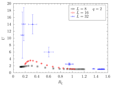
Figure 3: $N=2$, $q=2$, $\kappa=0.04$. Behaviour of $U$ as a function of $R_{\xi}$, obtained by varying the parameter $J$ in the Hamiltonian.

Figure 4: $N=2$, $q=2$, $\kappa=0.04$. Histograms of the scalar part of energy density $H_{z}/L^{3}$ for $J\simeq 0.602$.

We then move to the large $\kappa$ side of the phase diagram by fixing $\kappa=0.4$, a value larger than $\kappa_{c}^{\mathbb{Z}_{q}}(J=0)\approx 0.3$ (see Eq. 12). In this case a transition in the O(4) universality class is found, as can be seen from Fig. 5, where the universal scaling curve obtained is compared to that of the O(4) model obtained by fixing $A_{{\bm{x}},\mu}=0$. Fitting the behavior of $R_{\xi}$ using the known critical exponent $\nu$ of the O(4) model, see Tab. 1, we obtain for the critical coupling the estimate $J_{c}=0.23433(5)$. This is only slightly larger than the critical coupling $J_{c}^{\mathrm{O(4)}}=0.233965(2)$ of the O(4) model, see Ref. Ballesteros:1996bd where the critical value of $2NJ$ is reported.

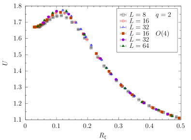
Figure 5: $N=2$, $q=2$, $\kappa=0.4$. Behaviour of $U$ as a function of $R_{\xi}$, obtained by varying the parameter $J$ in the Hamiltonian.

To complete our preliminary scan of the phase diagram of the $q=2$ model, and identify the $M_{2}M_{3}$ line in Fig. 2, we finally perform simulations fixing $J=0.2$ (a value smaller than $J_{c}$ at $\kappa=0.4$ and $\kappa=\infty$) and $J=1$ (a value larger than $J_{c}$ at $\kappa=0.04$). In both the cases transitions of the O(2) universality class are found, as can be seen from the FSS results shown in Fig. 6, obtained by using the known value of the O(2) exponent $\nu$, see Tab. 1. For $J=0.2$ no scaling violations are observed and the transition is located at $\kappa_{c}=0.2998(7)$; for $J=1$ scaling violations are sizable, and by excluding the $L=8$ lattice data from the fit we estimate the critical coupling to be $\kappa_{c}=0.0763(4)$. Both these values are quite close to their asymptotic values for $J=0$ and $J=\infty$ respectively, see Eqs. (11)-(12), signaling that the transition lines emerging from the $J=0$ and $J=\infty$ sides of the phase diagram are almost vertical.

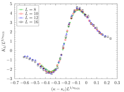
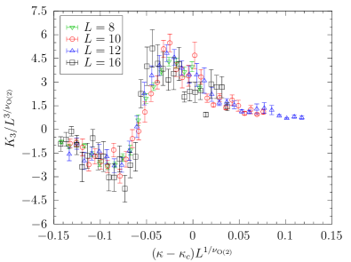
Figure 6: $N=2$, $q=2$. Finite size scaling of the third cumulant $K_{3}$, obtained by using the known O(2) value of the critical exponent $\nu$ (top) for $J=0.2$, with $\kappa_{c}=0.2998(7)$ (bottom) for $J=1$, with $\kappa_{c}=0.0763(4)$.

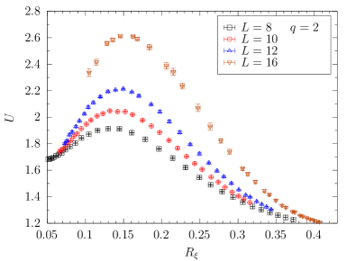
Figure 7: $N=2$, $q=2$, $\kappa=0.275$. Behaviour of $U$ as a function of $R_{\xi}$, obtained by varying the parameter $J$ in the Hamiltonian.

Figure 8: $N=2$, $q=2$, $\kappa=0.275$. Histograms of the scalar part of energy density $H_{z}/L^{3}$ for $J\simeq 0.256$.

We finally perform a simulation fixing $\kappa=0.275$, in order to cross the $M_{2}M_{3}$ line in Fig. 2. The results obtained for $U$ as a function of $R_{\xi}$ are shown in Fig. 7: data corresponding to different values of the lattice size $L$ do not collapse on each other, and the peak values of $U$ at fixed $L$ increase significantly by increasing $L$. We thus expect in this case the presence of a first order transition, which is confirmed by the emergence of a double peak structure in the energy density $H_{z}/L^{3}$ when increasing the lattice size, see Fig. 8.

We can thus conclude that the phase diagram of the model with $q=2$ is fully consistent with the one sketched in Fig. 2, with the possibly interesting $M_{2}M_{3}$ line being a line of first order phase transitions.

To close this section we present results obtained along the $M_{2}M_{3}$ line, always at $\kappa=0.275$, for $q=3$ and $q=9$. In both the cases first order phase transitions are found, as seen from Figs. 9: no scaling is observed in the $U$ vs $R_{\xi}$ plot, however the strength of the first order transition decreases when increasing $q$, and for $q=9$ data are practically indistinguishable from those of the U(1)^(nc) model, in which a very weak first order phase transition is present for $N=2$, see Refs. KMPST-08 ; Bonati:2020jlm .

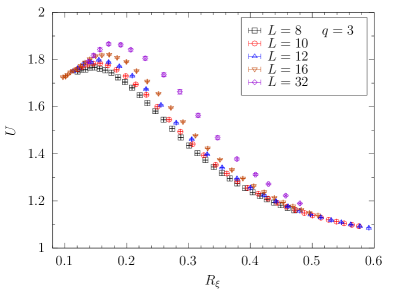
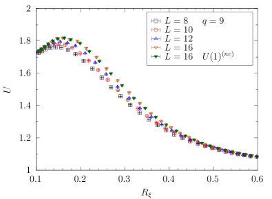
Figure 9: $N=2$, $\kappa=0.275$. Behaviour of $U$ as a function of $R_{\xi}$, obtained by varying the parameter $J$ in the Hamiltonian for the model with $q=3$ (top) and $q=9$ (bottom). In the latter case data for the U(1)^(nc) model are also shown for comparison.

III.3 The case $N=25$

We now discuss the results obtained for the model with $25$ scalar flavours, starting again from the $q=2$ gauge discretization and focussing on the most interesting part of the phase diagram.

Figure 10: $N=25$, $q=2$, $\kappa=0.4$. Behaviour of $U$ as a function of $R_{\xi}$, obtained by varying the parameter $J$ in the Hamiltonian.

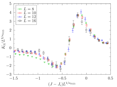
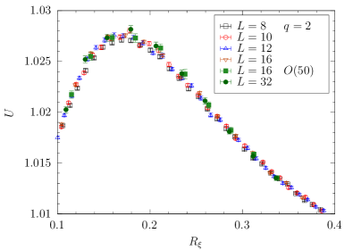
Figure 11: $N=25$, $q=2$, $\kappa=0.275$. (top) Finite size scaling of the third cumulant $K_{3}$, obtained by using the known O(2) value of the critical exponent $\nu$ and $J_{c}=0.181(2)$. (bottom) Behaviour of $U$ as a function of $R_{\xi}$, obtained by varying the parameter $J$ in the Hamiltonian.

We first of all present the results obtained for $\kappa=0.4$ (larger than $\kappa^{\mathbb{Z_{q}}}_{c}(J=0)\approx 0.3$, see Eq. (12)), where a transition of the O(50) universality class is expected. Results reported in Fig. 10 are fully consistent with this expectation, since the scaling curve obtained for $U$ against $R_{\xi}$ is well compatible with the one of the O(50) model, determined by fixing $A_{{\bm{x}},\mu}\equiv 0$ in the simulations. To fit the behavior of $R_{\xi}$ we use the large $N$ prediction of $\nu$ reported in the caption of Tab. 1, obtaininig the estimate $J_{c}=0.2502(3)$ for the critical coupling. This value is already quite close to the asymptotic large $N$ critical coupling of the O(N) models, $J_{c}=0.252731\ldots$, reported in Ref. Campostrini:1995np .

Figure 12: $N=25$, $q=3$, $\kappa=0.275$. Histograms of the scalar part of energy density $H_{z}/L^{3}$ for $J\simeq 0.267$.

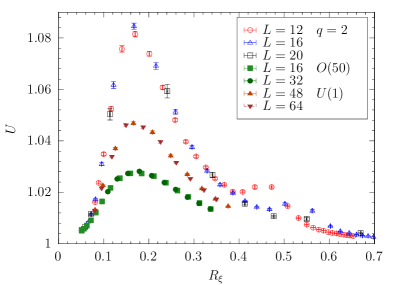
Figure 13: $N=25$, $q=4$, $\kappa=0.275$. Behaviour of $U$ as a function of $R_{\xi}$, obtained by varying the parameter $J$ in the Hamiltonian. For comparison data for the O(50) and the U(1)^(nc) models from Ref. Bonati:2020jlm are also reported.

Other simulations have been performed at $\kappa=0.275$, which is smaller than $\kappa^{\mathbb{Z}_{q}}_{c}(J=0)\approx 0.3$. However for $N=25,q=2$ the transition line emerging from the $J=0$ critical point is not vertical anymore, and in this case we found two transitions: an O(2) transition at $J_{c}=0.181(2)$ and an O(50) transition at $J_{c}=0.2506(3)$, as can be seen from the FSS curves shown in Fig. 11. To approximately locate the position of the multicritical point $M_{3}$ in Fig. 2, we thus performed simulations at fixed $J=0.2$, finding an O(2) transition at $\kappa_{c}=0.2554(15)$. Simulations at fixed $\kappa=0.2$ show evidence of two very close transitions at $J_{c}\approx 0.2518$, providing our best estimate for the position of the multicritical point $M_{3}$. Finally, simulations performed at $\kappa=0.15$ found a first order transition at $J\approx 0.25$, with hints of a continuous transition for slightly larger values of the coupling $J$; it is thus possible that this point is on the left of the multicrical point $M_{2}$ in Fig. 2, or anyway very close to it.

The region $M_{2}M_{3}$ is thus quite small for $N=25$, $q=2$, and significant crossover effects are expected to be found due to the nearby O(50) and first order transition lines. Since a complete investigation of the small $q$ case is not our principal aim, we leave a detailed analysis of this region of the parameter space to future studies.

The model with $N=25$, $q=3$ is much simpler: in this case $\kappa_{c}^{\mathbb{Z}_{q}}(J=0)\approx 0.68$ (see Eq. 12), and by performing simulations at $\kappa=0.7$ a clear O(50) transition is found for $J_{c}=0.25051(15)$. However simulations at $\kappa=0.275$ provide clear evidence of a strong first order phase transition for $J_{c}\simeq 0.267$, see the histograms reported in Fig. 12.

The interpretation of the case $N=25$, $q=4$ is again problematic: now $\kappa_{c}^{\mathbb{Z}_{q}}(J=0)\approx 1.2$ (see Eq. 12), but the results of simulations performed both at $\kappa=0.4$ and $\kappa=0.275$ do not provide clear indications on the nature of the critical behavior. In both the cases very large correction to scaling are found, with data for $U$ against $R_{\xi}$ that seem to approach an asymptotic curve that does not correspond neither to the Abelian Higgs nor the O(50) universality classes, see Fig. 13 for the $\kappa=0.275$ case. To make things worst, the apparent asymptotic curve of the $\kappa=0.275$ data is different from the one obtained for $\kappa=0.4$. The most natural interpretation of these results is that much larger lattices would be needed to really resolve the true critical behavior of the model.

Figure 14: $N=25$, $q=5$, $J=0.2$. Finite size scaling of the third cumulant $K_{3}$, obtained by using the known O(2) value of the critical exponent $\nu$ and $\kappa_{c}=1.792(1)$.

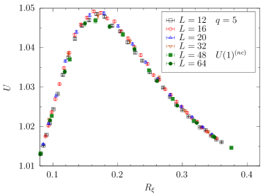
Figure 15: $N=25$, $q=5$, $\kappa=0.4$. Behaviour of $U$ as a function of $R_{\xi}$, obtained by varying the parameter $J$ in the Hamiltonian. For comparison data for the U(1)^(nc) model from Ref. Bonati:2020jlm are also reported.

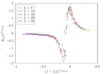
Figure 16: $N=25$, $q=5$, $\kappa=1.2$. Finite size scaling of the third cumulant $K_{3}$, obtained by using the known O(2) value of the critical exponent $\nu$ and $J_{c}=0.2727$ ($L=8$ was not included in the fit to determine $J_{c}$).

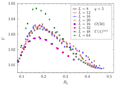
Figure 17: $N=25$, $q=5$, $\kappa=1.2$. Behaviour of $U$ as a function of $R_{\xi}$, obtained by varying the parameter $J$ in the Hamiltonian. For comparison data for the O(50) and U(1)^(nc) models from Ref. Bonati:2020jlm are also reported.

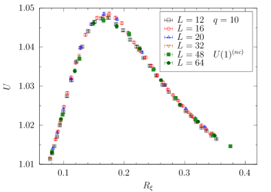
Figure 18: $N=25$, $q=10$, $\kappa=0.4$. Behaviour of $U$ as a function of $R_{\xi}$, obtained by varying the parameter $J$ in the Hamiltonian. For comparison data for the U(1)^(nc) model from Ref. Bonati:2020jlm are also reported.

The model with $N=25$, $q=5$ turns out to be the most interesting one. For this model $\kappa_{c}^{\mathbb{Z}_{q}}(J=0)\approx 1.9$ (see Eq. 12), and by performing simulations at $J=0.2$ and $J=0.25$ we find clear O(2) transitions at $\kappa_{c}=1.792(1)$ and $\kappa_{c}=1.509(2)$ respectively, see Fig. 14 for the case $J=0.2$. Fixing $\kappa=0.4$ and scanning in the coupling $J$ we find the symmetry enlargement we were looking for: the universal scaling curve of $U$ against $R_{\xi}$ is indeed the same as that of the U(1)^(nc) model, as can be appreciated from data reported in Fig. 15. By using the critical exponent $\nu$ reported in Tab. 1 for the Abelian Higgs universality class, we obtain for the critical coupling the estimate $J_{c}=0.29509(2)$, which is already remarkably close to the critical coupling $J_{c}^{U(1)}=0.295511(4)$ of the U(1)^(nc) model with $N=25$ for $\kappa=0.4$ (see Ref. Bonati:2020jlm ).

Simulations of the $N=25$, $q=5$ model have been carried out also for $\kappa=1.2$, which turned out to be quite close to the multicritical point $M_{3}$ in Fig. 2. Two nearby transitions can indeed be found at $J_{c}\approx 0.2674$ and $J_{c}\approx 0.2727$, detected by using $R_{\xi}$ and $U$, and $K_{3}$ respectively. The scaling of $K_{3}$ at the transition with $J_{c}\approx 0.2727$ is consistent with the exponents of the O(2) universality class, see Fig. 16 ($L=8$ was not included in the fit for find $J_{c}$). The scaling of $U$ against $R_{\xi}$ at $J_{c}\approx 0.2674$ is instead nontrivial, as can be seen from Fig. 17. Data seems to collapse on a common scaling curve, although significant corrections to scaling are present, especially in the right part of the figure, where a contamination coming from the second transition is present. The significant thing to note is that this scaling curve is however different from universal curves of the O(50) and of the U(1)^(nc) models, also shown in Fig. 17. This behavior can be explained in a natural way by assuming the multicritical point $M_{3}$ to be associated to a continuous transition, whose scaling function is the one on which data points in Fig. 17 collapse, due to a crossover phenomenon.

Finally, to verify that the symmetry enlargement observed for $q=5$ is present also for larger values of the discretization parameter, we present results obtained for the model with $q=10$, again for $\kappa=0.4$. As expected, also in this case the symmetry enlargement to the Abelian Higgs universality class is present, as can be seen from Fig. 18. In this case the transition is located at $J_{c}=0.29555(2)$ which is only two standard deviations away from the value $J_{c}^{U(1)}=0.295511(4)$ obtained in Ref. Bonati:2020jlm in the U(1)^(nc) model.

IV Conclusions

In this work we studied a variant of the non-compact multicomponent lattice Abelian Higgs model with reduced gauge symmetry, with the aim of investigating whether the discrete $\mathbb{Z}_{q}^{(nc)}=2\pi\mathbb{Z}/q$ gauge symmetry is sufficient for the model to display transitions in the continuous Abelian Higgs universality class.

In studying this model we considered two different values for the number of scalar flavors, namely $N=2$ and $N=25$. Although the topology of the phase diagram is the same in these two cases, the universality classes of the transitions present in these two cases are very different. Indeed the results obtained in the model with gauge symmetry $\mathbb{Z}_{q}^{(nc)}$ are expected to converge, for large $q$, to those of the model with gauge symmetry U(1)^(nc), and only for large enough $N$ the U(1)^(nc) model exhibit transitions in which both gauge and scalar degrees of freedom become critical MV-08 ; KMPST-08 ; Bonati:2020jlm .

We thus verified that for $N=2$ the numerical results are consistent with the absence of any symmetry enlargement, since both the $\mathbb{Z}_{q}^{(nc)}$ and the U(1)^(nc) gauge theories display first order phase transitions in large parts of the phase diagram.

The case $N=25$ is clearly the most interesting one. The analysis of the values $q=2$ and $q=4$ of the gauge discretization parameter can not be considered conclusive, since large crossover effects seem to be present. For $q\geq 5$, instead, we unambiguously identified regions of the parameter space in which the $\mathbb{Z}_{q}^{(nc)}$ gauge symmetry enlarges to U(1)^(nc), and the model with discrete gauge group exhibits transitions of the continuous Abelian Higgs universality class.

This is not incompatible with the negative results recently obtained in Ref. discretecompact , where an analogous discretization of the compact Abelian Higgs model with charge $Q=2$ has been studied, since the presence of first order phase transitions can never be excluded by universality arguments alone. However, it will be surely interesting to understand, in future studies, the dynamical origin of this difference, to better understand the relation between the compact and the non-compact models Bonati:2020jlm ; Bonati:2020ssr ; Bonati:2022oez . In particular, it is still an open question whether transitions of the continuous Abelian Higgs universality class are possible in a lattice model with a finite Abelian gauge group, like the one studied in Ref. discretecompact but unlike the one used in the present work (which is discrete but infinite).

We finally note that the results obtain at $N=25$, $q=5$ for $\kappa=1.2$ suggest the multicritical point $M_{3}$ in Fig. 2 to be associated to a continuous phase transition. This is something that surely deserves to be further investigated, both from the numerical and from the analytical point of view. Such a continuous transition would indeed correspond to a very peculiar multicritical theory, with lines of O(2N), Abelian Higgs and O(2) (ordinary and topological) transitions crossing each other.

Acknowledgement. Numerical simulations have been performed on the CSN4 cluster of the Scientific Computing Center at INFN-PISA. It is a pleasure to thank A. Pelissetto and E. Vicari for discussions and comments.

References

- (1) L. D. Landau and E. M. Lifshitz Statistical Physics, Part 1 Volume 5 of Course of Theoretical Physics (Pergamonn Press, Oxford, UK, 1980)
- (2) P. W. Anderson, Basic Notions of Condensed MatterPhysics, (The Benjamin/Cummings Publishing Company, Menlo Park, California, 1984)
- (3) K. G. Wilson and J. B. Kogut, “The Renormalization group and the epsilon expansion,” Phys. Rept. 12, 75 (1974).
- (4) J. Zinn-Justin, Quantum Field Theory and Critical Phenomena, fourth edition (Clarendon Press, Oxfrd, UK, 2002)
- (5) A. Pelissetto and E. Vicari, “Critical phenomena and renormalization group theory,” Phys. Rept. 368, 549 (2002) [arXiv:cond-mat/0012164 [cond-mat]].
- (6) J. Hove and A. Sudbo, “Criticality versus q in the 2+1-dimensional Z(q) clock model,” Phys. Rev. E 68, 046107 (2003) [arXiv:cond-mat/0301499 [cond-mat.stat-mech]].
- (7) M. Hasenbusch, “Monte Carlo study of an improved clock model in three dimensions,” Phys. Rev. B 100, 224517 (2019) [arXiv:1910.05916 [cond-mat.stat-mech]].
- (8) M. Hasenbusch, “Monte Carlo study of a generalized icosahedral model on the simple cubic lattice,” Phys. Rev. B 102, 024406 (2020) [arXiv:2005.04448 [cond-mat.stat-mech]].
- (9) S. Weinberg, The Quantum Theory of Fields, (Cambridge University Press, Cambridge, UK, 2005)
- (10) E. Fradkin Field Theories of Condensed Matter Physics (Cambridge University Press, Cambridge, UK, 2013).
- (11) R. Moessner, J. E. Moore Topological Phases of Matter (Cambridge University Press, Cambridge, UK, 2021).
- (12) S. Sachdev, “Topological order, emergent gauge fields, and Fermi surface reconstruction,” Rept. Prog. Phys. 82, 014001 (2019) [arXiv:1801.01125 [cond-mat.str-el]].
- (13) R. D. Pisarski and F. Wilczek, “Remarks on the Chiral Phase Transition in Chromodynamics,” Phys. Rev. D 29, 338 (1984).
- (14) K. Rajagopal and F. Wilczek, “The Condensed matter physics of QCD,” in M. Shifman, B. Ioffe (ed.) At the frontier of particle physics. Handbook of QCD. Vol. 1-3 (World Scientific, Singapore, Singapore, 2001) [arXiv:hep-ph/0011333 [hep-ph]].
- (15) E. H. Fradkin and S. H. Shenker, “Phase Diagrams of Lattice Gauge Theories with Higgs Fields,” Phys. Rev. D 19, 3682 (1979).
- (16) A. Pelissetto and E. Vicari, “Three-dimensional ferromagnetic CP(N-1) models,” Phys. Rev. E 100, 022122 (2019) [arXiv:1905.03307 [cond-mat.stat-mech]].
- (17) A. Pelissetto and E. Vicari, “Large- behavior of three-dimensional lattice CPN-1 models,” J. Stat. Mech. 2003, 033209 (2020)
- (18) A. Pelissetto and E. Vicari, “Multicomponent compact Abelian-Higgs lattice models,” Phys. Rev. E 100, 042134 (2019) [arXiv:1909.04137 [cond-mat.stat-mech]].
- (19) C. Bonati, A. Pelissetto and E. Vicari, “Multicritical point of the three-dimensional Z2 gauge Higgs model,” Phys. Rev. B 105, 165138 (2022) [arXiv:2112.01824 [cond-mat.stat-mech]].
- (20) C. Bonati, A. Pelissetto and E. Vicari, “Scalar gauge-Higgs models with discrete Abelian symmetry groups,” Phys. Rev. E 105, 054132 (2022) [arXiv:2204.02907 [cond-mat.stat-mech]].
- (21) C. Bonati, A. Pelissetto and E. Vicari, “Phase diagram, symmetry breaking, and critical behavior of three-dimensional lattice multiflavor scalar chromodynamics,” Phys. Rev. Lett. 123, 232002 (2019) [arXiv:1910.03965 [hep-lat]].
- (22) C. Bonati, A. Pelissetto and E. Vicari, “Three-dimensional lattice multiflavor scalar chromodynamics: interplay between global and gauge symmetries,” Phys. Rev. D 101, 034505 (2020) [arXiv:2001.01132 [cond-mat.stat-mech]].
- (23) C. Bonati, A. Franchi, A. Pelissetto and E. Vicari, “Three-dimensional lattice SU(Nc) gauge theories with multiflavor scalar fields in the adjoint representation,” Phys. Rev. B 104, 115166 (2021) [arXiv:2106.15152 [hep-lat]].
- (24) C. Bonati, A. Franchi, A. Pelissetto and E. Vicari, “Phase diagram and Higgs phases of three-dimensional lattice SU(Nc) gauge theories with multiparameter scalar potentials,” Phys. Rev. E 104, 064111 (2021) [arXiv:2110.01657 [cond-mat.stat-mech]].
- (25) F. J. Wegner, “Duality in Generalized Ising Models and Phase Transitions Without Local Order Parameters,” J. Math. Phys. 12, 2259 (1971).
- (26) R. Savit, “Duality in Field Theory and Statistical Systems,” Rev. Mod. Phys. 52, 453 (1980).
- (27) O. Borisenko, V. Chelnokov, G. Cortese, M. Gravina, A. Papa and I. Surzhikov, “Critical behavior of 3D Z(N) lattice gauge theories at zero temperature,” Nucl. Phys. B 879, 80 (2014) [arXiv:1310.5997 [hep-lat]].
- (28) O. I. Motrunich and A. Vishwanath, “Comparative study of Higgs transition in one-component and two-component lattice superconductor models,” [arXiv:0805.1494 [cond-mat.stat-mech]].
- (29) A. B. Kuklov, M. Matsumoto, N. V. Prokof’ev, B. V. Svistunov, and M. Troyer, “Deconfined Criticality: Generic First-Order Transition in the SU(2) Symmetry Case,” Phys. Rev. Lett. 101, 050405 (2008) [arXiv:0805.4334 [cond-mat.stat-mech]].
- (30) C. Bonati, A. Pelissetto and E. Vicari, “Lattice Abelian-Higgs model with noncompact gauge fields,” Phys. Rev. B 103, 085104 (2021) [arXiv:2010.06311 [cond-mat.stat-mech]].
- (31) C. Bonati, A. Pelissetto and E. Vicari, “Higher-charge three-dimensional compact lattice Abelian-Higgs models,” Phys. Rev. E 102, 062151 (2020) [arXiv:2011.04503 [cond-mat.stat-mech]].
- (32) C. Bonati, A. Pelissetto and E. Vicari, “Critical behaviors of lattice U(1) gauge models and three-dimensional Abelian-Higgs gauge field theory,” Phys. Rev. B 105, 085112 (2022) [arXiv:2201.01082 [cond-mat.stat-mech]].
- (33) C. Bonati and A. Franchi, “Color-flavor reflection in the continuum limit of two-dimensional lattice gauge theories with scalar fields,” Phys. Rev. E 105, no.5, 054117 (2022) [arXiv:2203.06979 [hep-lat]].
- (34) S. Sachdev, H. D. Scammell, M. S. Scheurer and G. Tarnopolsky, “Gauge theory for the cuprates near optimal doping,” Phys. Rev. B 99, 054516 (2019) [arXiv:1811.04930 [cond-mat.str-el]].
- (35) H. D. Scammell, K. Patekar, M. S. Scheurer and S. Sachdev, “Phases of SU(2) gauge theory with multiple adjoint Higgs fields in 2+1 dimensions,” Phys. Rev. B 101, 205124 (2020) [arXiv:1912.06108 [cond-mat.str-el]].
- (36) T. Senthil, L. Balents, S. Sachdev, A. Vishwanath and M. P. A. Fisher, “Quantum Criticality beyond the Landau-Ginzburg-Wilson Paradigm”, Phys. Rev. B 70, 144407 (2004) [arXiv:cond-mat/0312617 [cond-mat.str-el]].
- (37) G. Bracci-Testasecca and A. Pelissetto, “Multicomponent gauge-Higgs models with discrete Abelian gauge groups,” [arXiv:2211.01662 [hep-lat]].
- (38) L. D. McLerran and B. Svetitsky, “Quark Liberation at High Temperature: A Monte Carlo Study of SU(2) Gauge Theory,” Phys. Rev. D 24, 450 (1981).
- (39) B. Svetitsky and L. G. Yaffe, “Critical Behavior at Finite Temperature Confinement Transitions,” Nucl. Phys. B 210, 423 (1982).
- (40) A. S. Kronfeld and U. J. Wiese, “SU(N) gauge theories with C periodic boundary conditions. 1. Topological structure,” Nucl. Phys. B 357, 521 (1991)
- (41) C. Dasgupta and B. I. Halperin, “Phase Transition in a Lattice Model of Superconductivity,” Phys. Rev. Lett. 47, 1556 (1981).
- (42) T. Neuhaus, A. Rajantie and K. Rummukainen, “Numerical study of duality and universality in a frozen superconductor,” Phys. Rev. B 67, 014525 (2003) [arXiv:cond-mat/0205523 [cond-mat]].
- (43) B. I. Halperin, T. C. Lubensky, and S. K. Ma, “First-Order Phase Transitions in Superconductors and Smectic-A Liquid Crystals,” Phys. Rev. Lett. 32, 292 (1974).
- (44) V. Y. Irkhin, A. A. Katanin and M. I. Katsnelson, “1/N expansion for critical exponents of magnetic phase transitions in CP**(N-1) model at 2 d 4,” Phys. Rev. B 54, 11953 (1996) [arXiv:cond-mat/9703011 [cond-mat]].
- (45) M. Moshe and J. Zinn-Justin, “Quantum field theory in the large N limit: A Review,” Phys. Rept. 385, 69 (2003) [arXiv:hep-th/0306133 [hep-th]].
- (46) B. Ihrig, N. Zerf, P. Marquard, I. F. Herbut and M. M. Scherer, “Abelian Higgs model at four loops, fixed-point collision and deconfined criticality,” Phys. Rev. B 100, 134507 (2019) [arXiv:1907.08140 [cond-mat.str-el]].
- (47) J. Smiseth, E. Smorgrav, F. S. Nogueira, J. Hove and A. Sudbo, “Phase structure of d = 2+1 compact lattice gauge theories and the transition from Mott insulator to fractionalized insulator,” Phys. Rev. B 67, 205104 (2003) [arXiv:cond-mat/0301297 [cond-mat]].
- (48) M. S. S. Challa, D. P. Landau, and K. Binder, “Finite-size effects at temperature-driven first-order transitions,” Phys. Rev. B 34, 1841 (1986).
- (49) K. Vollmayr, J. D. Reger, M. Scheucher, and “K. Binder, Finite size effects at thermally-driven first order phase transitions: A phenomenological theory of the order parameter distribution,” Z. Phys. B 91, 113 (1993).
- (50) S. M. Chester, W. Landry, J. Liu, D. Poland, D. Simmons-Duffin, N. Su and A. Vichi, “Carving out OPE space and precise model critical exponents,” JHEP 06, 142 (2020) [arXiv:1912.03324 [hep-th]].
- (51) M. Hasenbusch and E. Vicari, “Anisotropic perturbations in three-dimensional O()-symmetric vector models,” Phys. Rev. B 84, 125136 (2011) [arXiv:1108.0491 [cond-mat.stat-mech]].
- (52) R. Guida and J. Zinn-Justin, “Critical exponents of the N vector model,” J. Phys. A 31, 8103 (1998) [arXiv:cond-mat/9803240 [cond-mat]].
- (53) F. Kos, D. Poland and D. Simmons-Duffin, “Bootstrapping the vector models,” JHEP 06, 091 (2014) [arXiv:1307.6856 [hep-th]].
- (54) J. A. Gracey, “Crossover exponent in O(N) phi**4 theory at O(1 / N**2),” Phys. Rev. E 66, 027102 (2002) [arXiv:cond-mat/0206098 [cond-mat]].
- (55) H. G. Ballesteros, L. A. Fernandez, V. Martin-Mayor and A. Munoz Sudupe, “Finite size effects on measures of critical exponents in d = 3 O(N) models,” Phys. Lett. B 387, 125 (1996) [arXiv:cond-mat/9606203 [cond-mat]].
- (56) M. Campostrini, A. Pelissetto, P. Rossi and E. Vicari, “Four point renormalized coupling constant in O(N) models,” Nucl. Phys. B 459, 207 (1996) [arXiv:hep-lat/9506002 [hep-lat]].