MARS: Message Passing for Antenna and RF Chain Selection for Hybrid Beamforming in MIMO Communication Systems

Abstract

In this paper, we consider a prospective receiving hybrid beamforming structure consisting of several radio frequency (RF) chains and abundant antenna elements in multi-input multi-output (MIMO) systems. Due to conventional costly full connections, we design an enhanced partially connected beamformer employing a low-density parity-check (LDPC)-based structure. As a benefit of the LDPC-based structure, information can be exchanged among clustered RF/antenna groups, which results in a low computational complexity order. Advanced message passing (MP) capable of inferring and transferring information among different paths is designed to support the LDPC-based hybrid beamformer. We propose a message-passing enhanced antenna and RF chain selection (MARS) scheme for minimizing the operational power of antennas and RF chains of the receiver. Furthermore, sequential and parallel MP schemes for MARS are designed, namely, MARS-S and MARS-P, respectively, to address the convergence speed issue. Simulations validate the convergence of both the MARS-P and the MARS-S algorithms. Due to the asynchronous information transfer of MARS-P, it requires higher power than MARS-S, which strikes a compelling balance among power consumption, convergence, and computational complexity. It is also demonstrated that the proposed MARS scheme outperforms the existing benchmarks using the heuristic method of fully/partially connected architectures in the open literature by requiring the lowest power and realizing the highest energy efficiency.

I Introduction

Wireless communication systems are experiencing revolutionary advances due to rapid changes in the creation and sharing of diverse information by human society. Abundant applications with exponentially high wireless traffic demands are emerging [1, 2]. In recent years, researchers have investigated promising technology for supporting advanced wireless communication systems with high spectral efficiency and energy efficiency (EE). A denser deployment of base stations (BSs) with a larger bandwidth can achieve high performance with increasing degrees of freedom from the perspective of hardware and radio resources but requires substantial consumption of electricity [3]. Accordingly, serious atmospheric pollution issues will arise due to global carbon emissions ascribed to the information and communications technology industry. Therefore, it would be beneficial if BSs were capable of efficiently employing low-power configurations to meet stringent service requirements and resiliently improve network performance [4].

As a prospect of wireless transmission systems, a massive multi-input multi-output (MIMO) system deployed within a BS is capable of transceiving enormous radio frequency (RF) signals, benefiting from its gains from multiplexing and diversity [5]. However, it potentially provokes power dissipation in MIMO due to diverse transmission directions. Therefore, the beamformer architecture of a MIMO system should be well established and appropriately designed to concentrate transmission power in certain directions [6]. Conventionally, there exist low-cost analog and high-performance digital beamforming techniques that can resolve the abovementioned issues [7]. Analog beamforming aims to adjust the phase shifters of antennas to perform directional data transfer while consuming few circuit power resources. However, limited selection of directional beams is intrinsically induced by the quantized phases from hardware constraints. In addition, digital beamforming can perform a more comprehensive task in terms of baseband interbeam interference cancellation, providing full management of directional beam coverage. Nevertheless, digital structure fundamentally requires a variety of RF chains connected to individual antennas, which requires substantial expenditure for configuration, power consumption and transceiver deployment. Therefore, the hybrid beamforming (HBF) architecture has become a promising and implementable solution by leveraging the advantages of both low-cost analog structures and highly directional digital structures [8]. Accordingly, fewer RF chains can be constructed to associate with enormous antennas, which reduces the cost while maintaining the asymptotic performance of digital beamforming.

In recent years, abundant research has focused on HBF architectural design but has been confined to specific structures, i.e., full connection and subconnection using separate subarrays [9, 10]. Due to the high degree of freedom of full connection in HBF, it enables the BS to achieve a nearly optimal solution. In [11], only analog beamforming, i.e., beam directions, is considered, which aims to maximize multi-device-based resource utilization. However, joint baseband digital and analog phase shifter precoders should be designed, which have considerably high computational complexity [12]. In [13, 14], beamforming schemes were designed from protocol perspectives. Although deep learning can alleviate the complexity issue, it cannot derive either closed forms or proofs of optimality or convergence [15]. Accordingly, some papers focused on designs of a disjoint solution of analog and digital beamforming under the conventional fully connected HBF architecture [16, 17]. For separate subarrays in HBF, RF chains take control of independent subsets of phase shifters and antenna elements. In surveys [9, 10], the authors investigated many subconnection architectures of HBF. In [18], the authors design a disjoint analog/digital beamforming for subarray architectures. Nonetheless, the performance of subarrays is potentially limited due to the inflexibility and inaccessibility of information from other RF chains or antenna sets. In [19], low-resolution quantizers of digital-to-analog converters were adopted in partially-connected HBF architecture for improving system spectral efficiency. In [20], partially-connected HBF is designed for advanced applications for multiuser integrated sensing and communication systems. In [21], the bit error rate was minimized under various RF/antenna connections. Therefore, it becomes compellingly important to design a novel HBF architecture to achieve the benefits of high operational flexibility and asymptotic performance of digital beamforming.

However, increasingly large-scale HBF architectures with enormous antennas and RF chains serving multiple devices will lead to substantially high overhead in terms of power and complexity, which has almost not been discussed or optimized in the abovementioned works [11, 12, 13, 14, 15, 16, 17, 18, 21]. In [22], the authors discussed different RF connections for subarray-based hybrid beamformers. The power consumption factor under each architecture was also analyzed. In [23], a generalized subarray-connected architecture was introduced for improving the EE in HBF, which aims to solve rate optimization problems with each subproblem related to a single subarray. A dynamic adjustment of the subarray architecture under partial connections was designed to achieve high EE performance [23]. In [24, 25, 26, 27], the authors addressed the importance of optimizing EE from either an architectural or hardware perspective. The operating power amplifiers and transmit power were considered in [24, 25] but without consideration of RF/antenna effects, which were taken into account in [26, 27]. However, all of these studies focused on fully connected HBF architectures optimizing EE, which requires high complexity. To elaborate further, conventional HBF architecture with high power consumption may be inappropriate for the future promising applications in joint radar sensing and communication systems [28, 29]. Moreover, under such architectures, it is unnecessary for all RF chains and antennas to be operated due to worse channel conditions and high power consumption, which should be appropriately selected to prevent performance degradation. In [30], antenna selection methods were designed for full-connection HBF maximizing the overall data rate. On the other hand, [31, 32] performed RF chain selection in a fully connected HBF architecture by optimizing energy utilization. However, none of these studies considered the joint selection of RF chains or antennas, which is capable of supporting potentially resilient beamforming with high EE. Accordingly, the joint design of RF/antenna selection and power consumption, as well as flexible HBF architectures, should be considered.

In a flexible HBF architecture, RF chains are partially connected to the corresponding antenna sets. However, some direct links between RF chains and antennas do not exist, which potentially induces information vanishing. Message passing (MP), which originated from factor graph theory [33], is deemed a prospective technique for large-scale networking, which possesses the capability to transfer desirable data^I and information among enormous links and nodes [34, 35]. In [36], MP-aided subarray-based link optimization was resolved, whereas the power allocation problem for beamforming was considered by MP in [37]. In [38], MP-based receiving beamforming was designed under full connection, while antenna selection using MP was developed in [39]. However, the joint design of a partially connected HBF architecture and RF/antenna selection has not been studied in previous works. Benefitting from resilient HBF, MP is particularly suitable for partially connected HBF architectures with indirect links. The policy and determination of RF sets can be readily passed through HBF links to the corresponding antenna sets. However, under a flexible HBF connection architecture, partial links potentially lead to unreachable information between faraway nodes, and it becomes compellingly imperative to design a novel HBF architecture.

Inspired by the concept of low-density parity-check (LDPC) [40] coding, the HBF architecture is redesigned to ensure that different sets become dependent with the fewest links [41]. In other words, information can be definitely conveyed from one set to the other within polynomial time, which is not considered in existing HBF architecture design. Moreover, under the partial connections of LDPC coding, MP can effectively and efficiently convey policies among RF/antenna nodes in HBF. Accordingly, we design a novel flexible HBF architecture by employing an LDPC-based structure considering the minimization of power consumption and RF/antenna selection in a massive MIMO communication system. The contributions of this work are summarized as follows.

$\bullet$

We design an LDPC-based connection for an HBF structure considering antenna and RF chain selection at the receiver. Compared with a fully connected beamformer, each RF chain is partially connected to a cluster of antennas. For arbitrary pairs of RF chains or antennas, we prove that there exists at least one path that can transfer information from one set to the other within polynomial time, i.e., all RF/antenna sets at the receiver are dependent on the LDPC-based connection, unlike in existing partially connected beamformers.

$\bullet$

We simultaneously consider both antenna and RF chain selections at the receiver, which have not been jointly designed in the literature. We aim to minimize the receiver power consumption constrained by the minimum transmission data rate and the maximum tolerable system power usage. The formulated problem is decomposed into a pair of subproblems considering the selection of antennas and RF chains at the receiver, which are computed separately in each virtual processing controller depending on the exchanged message.

$\bullet$

We propose a message-passing enhanced antenna and RF chain selection (MARS) scheme to minimize the operational circuit power of antennas and RF chains of receiving hybrid beamformers. Sequential and parallel MP schemes for MARS are designed, namely, MARS-S and MARS-P, respectively. The antenna/RF virtual controller employing MARS-S passes the determined solutions in a sequential manner, while candidate outcomes of MARS-P are simultaneously transmitted to neighboring RF/antenna nodes. Considering computational complexity and convergence issues, MARS can be iteratively performed in either a centralized or distributed manner. In a centralized architecture, more RF/antenna nodes are clustered and managed by an RF/antenna virtual controller than in a distributed system.

$\bullet$

We evaluate the system performance of the proposed MARS scheme employing LPDC-based connections in receiving HBF under both centralized and distributed architectures. We quantify the power consumption and corresponding EE with respect to different quality-of-service (QoS) values, numbers of clustered RF/antenna nodes and connections, and insertion loss values between RF chains and antenna elements. The proposed MARS scheme outperforms existing techniques by realizing lower power consumption and higher EE.

Notations: We define bold capital letter $\mathbf{A}$ as a matrix, bold lowercase letter $\mathbf{a}$ as a vector, and $\mathcal{A}$ as a set. $[\mathbf{A}]_{mn}$ denotes the $(m,n)$-th element of matrix $\mathbf{A}$. Matrix operations $\mathbf{A}^{H}$ and $\mathbf{A}^{-1}$ represent the Hermitian transpose and inverse of $\mathbf{A}$. $\det(\cdot)$, $\operatorname{diag}(\cdot)$ and $\mathbbm{E}[\cdot]$ are defined as the determinant, diagonal matrix and expectation operation, respectively. $\mathbbm{1}(\mathcal{X})$ denotes an indicator function that is one when event $\mathcal{X}$ takes place. The operations $\neg$, $\land$, $\lor$ and $\oplus$ indicate the binarywise logical operations NOT, AND, OR and exclusive-OR, respectively. Additionally, $\bigvee$ denotes the sequential logic operations of $\lor$, i.e., $\bigvee_{i=1}^{N_{x}}x_{i}=x_{1}\lor x_{2}...\lor x_{N}$, where $N_{x}$ is the dimension of $\{x_{i}\}$. $\text{mod}(a,b)$ is the modulus operation with arbitrary integers $a$ and $b$, e.g., $\text{mod}(a,b)=0$ indicates that $a$ is an integer multiple of $b$. $\left\lceil\cdot\right\rceil$ is a ceiling function.

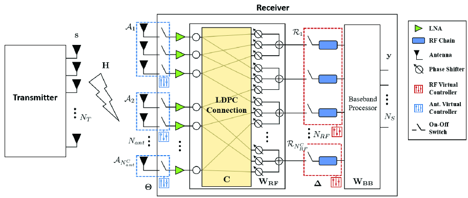
Figure 1: Proposed structure of the antenna and RF chain selection for hybrid beamforming in uplink.

II System Model and Problem Formulation

II-A System Model

We consider a partially connected HBF architecture at the receiving BS in an uplink massive MIMO communication system, as shown in Fig. 1. The receiving BS is equipped with RF chains $\mathcal{R}\in\{1,...,n,...,N_{RF}\}$ and antenna elements $\mathcal{A}\in\{1,...,m,...,N_{ant}\}$, where $N_{RF}$ and $N_{ant}$ indicate the total numbers of HBF RF chains and antennas, respectively. Without loss of generality, we assume that the hybrid beamformer possesses fewer RF chains than antennas due to the reduction in hardware expenditure in the fully digital beamformer, i.e., $N_{RF}\leq N_{ant}$. The receiving hybrid beamformer consists of an analog beamformer $\mathbf{{W}_{RF}}\in{\mathbbm{C}}^{N_{RF}\times N_{ant}}$ and a baseband digital beamformer $\mathbf{{W}_{BB}}\in{\mathbbm{C}}^{N_{S}\times N_{RF}}$, where $N_{S}$ denotes the number of data streams. The connection $\mathbf{C}\in{\mathbbm{Z}}^{N_{RF}\times N_{ant}}$ between the analog and baseband beamformers can be either in a full or partial connection, where ${[\mathbf{C}]}_{nm}\in\{0,1\},\forall n,m,$ indicates whether the $n$-th RF chain is linked to the $m$-th antenna. The desired transmitted signal is defined as $\mathbf{s}\in{\mathbb{C}}^{N_{T}\times 1}$, where $N_{T}$ is the number of antennas at the transmit BS.

To manage the energy consumption of HBF, we can switch off spoiled RF chains or antennas to optimize the power utilization. The selection matrices of RF chains and antenna elements are denoted by $\mathbf{\Delta}=\operatorname{diag}(\boldsymbol{\delta})=\operatorname{diag}(\delta_{1},...,\delta_{n},...,\delta_{N_{RF}})$ and $\mathbf{\Theta}=\operatorname{diag}(\boldsymbol{\theta})=\operatorname{diag}(\theta_{1},...,\theta_{m},...,\theta_{N_{ant}})$, respectively, where $\delta_{n}\in\{0,1\}$ and $\theta_{m}\in\{0,1\}$ indicate the selection decisions for RF chains and antennas, e.g., $\delta_{n}=1$ and $\theta_{m}=1$ mean that the $n$-th RF chain and $m$-th antenna are selected to be turned on. Since we focus on the designs at the receiving hybrid beamformer, the transmission power $P_{T}$ is considered to be equally allocated to transmit antennas^II-A, i.e., $\mathbbm{E}\left[\mathbf{s}{\mathbf{s}}^{H}\right]\!=\!\frac{P_{T}}{N_{T}}\mathbf{I}_{N_{T}}$, where $\mathbf{I}_{N_{T}}$ is the identity matrix of size $N_{T}$. The received uplink signal is given by

$$\mathbf{y}=\sqrt{\rho\left(1-\beta\right)}\mathbf{W_{BB}\Delta\left(C\circ W_{RF}\right)\Theta Hs\!+\!W_{BB}\left(C\circ W_{RF}\right)n},$$ (1)

where $\circ$ is the Hadamard product for elementwise multiplication. In $\eqref{recvsignal}$, $\rho$ is the distance-based loss and $\mathbf{H}\in\mathbb{C}^{N_{ant}\times N_{T}}$ is the small-scale fading channel, which is defined based on the Saleh Valenzuela model [18, 25] as

$$\mathbf{H}=\sqrt{\frac{N_{T}N_{ant}}{L}}\sum_{\ell=1}^{L}{\alpha}_{\ell}\cdot\boldsymbol{\alpha}_{r}({\phi}_{\ell}^{r})\boldsymbol{\alpha}_{t}^{H}({\phi}_{\ell}^{t}),$$ (2)

where $L$ is the number of multipaths and ${\alpha}_{\ell}\sim\mathcal{CN}(0,1)$ is the complex channel gain of the $\ell$-th path. The array response vector corresponding to the angle of arrival (AoA) of the HBF receiver and the angle of departure (AoD) of the transmit BS are given by $\boldsymbol{\alpha}_{r}({\phi}_{\ell}^{r})$ and $\boldsymbol{\alpha}_{t}({\phi}_{\ell}^{t})$, respectively, along with their incident receiving and transmit angles of ${\phi}_{\ell}^{r}$ and ${\phi}_{\ell}^{t}$. In $\eqref{recvsignal}$, $\mathbf{n}\!\sim\!\mathcal{CN}(0,N_{0}\mathbf{I}_{N_{R}})$ is complex additive white Gaussian noise with a noise power spectral density of $N_{0}$. Furthermore, we consider the insertion loss $\beta$ in the uplink receiving HBF-based BS [42], which is the connection loss between an RF chain and its connected antenna elements due to signal power dissipation. Based on the received uplink signal in $\eqref{recvsignal}$, the achievable system rate can be written as

$$R(\mathbf{\Delta,\Theta})\!=\!\log_{2} \left[\det\left|\mathbf{I}_{N_{S}}\!+\!\frac{P_{T}\rho\left(1-\beta\right)}{N_{0}N_{T}}\mathbf{W_{BB}\Delta\left(C\circ W_{RF}\right)\Theta H}\mathbf{H}^{H}\right.\right.$$

$$\left.\left.\mathbf{\Theta}^{H}\mathbf{W}^{H}_{\mathbf{RF}}\mathbf{\Delta}^{H}\mathbf{W}^{H}_{\mathbf{BB}}\left(\mathbf{W_{BB}\left(C\circ W_{RF}\right)}\mathbf{W}^{H}_{\mathbf{RF}}\mathbf{W}^{H}_{\mathbf{BB}}\right)^{-1}\right|\right].$$ (3)

The total power consumption at the receiver HBF-based BS can be represented by [25, 27]

$$P(\boldsymbol{\delta},\boldsymbol{\theta})=P_{BB}+\sum_{n=1}^{N_{RF}}\left[{\delta}_{n}\left(P_{RF}+P_{ADC}\right)+\sum_{m=1}^{N_{ant}}\left({\theta}_{m}P_{LNA}+[\mathbf{C}]_{nm}{\delta}_{n}{\theta}_{m}P_{PS}\right)\right],$$ (4)

where $P_{BB}$, $P_{RF}$, $P_{ADC}$, $P_{LNA}$ and $P_{PS}$ denote the circuit powers of HBF baseband signal processing, operations of RF chains, analog-to-digital converter, low-noise power amplifiers and phase shifters at receiving antennas, respectively. We observe that $\eqref{powerconsumption}$ includes a static power term $P_{BB}$ and dynamic power terms $P_{RF}$, $P_{ADC}$, $P_{LNA}$ and $P_{PS}$ because the dynamic terms are determined by the selection of RF chains and antennas. The system parameters and corresponding notations are listed in Table I.

TABLE I: Definition of System Parameters

Parameter	Notation
Sets of antennas and RF chains	$\mathcal{A},\mathcal{R}$
Numbers of transmitting and receiving antennas and RF chains	$N_{T},N_{ant},N_{RF}$
Number of data streams	$N_{S}$
HBF analog and baseband beamformers	$\mathbf{{W}_{RF}},\mathbf{{W}_{BB}}$
HBF connection	$\mathbf{C}$
RF chain and antenna selection matrices of	$\mathbf{\Delta},\mathbf{\Theta}$
RF chain and antenna element-wise selection	$\delta_{n},\theta_{m}$
Transmit, received, and noise signals	$\mathbf{s},\mathbf{y},\mathbf{n}$
Transmit power	$P_{T}$
Noise power	$N_{0}$
Small- and large-scale channel fading	$\mathbf{H},\rho$
Antenna gain function	${\Lambda}({\phi}_{\ell})$
Number of multipaths	$L$
Insertion loss	$\beta$
Achievable rate	$R(\mathbf{\Delta},\mathbf{\Theta})$
Total power consumption	$P(\boldsymbol{\delta},\boldsymbol{\theta})$
Baseband, RF, LNA, and phase shifter powers	$P_{B\!B},P_{R\!F},P_{L\!N\!A},P_{P\!S}$
Number of LDPC connections	$N_{Conn}$
Sets of RF and antenna controllers	$\mathcal{R}^{\mathcal{C}},\mathcal{A}^{\mathcal{C}}$
$k$-th RF and $l$-th antenna controller	$\mathcal{R}_{k},\mathcal{A}_{l}$
Numbers of RF and antenna controllers	$N_{RF}^{C},N_{ant}^{C}$
Numbers of RF and antenna elements controlled	$N_{RF,k},N_{ant,l}$
RF decision and antenna update sets of RF controllers	$\boldsymbol{\delta}_{\mathcal{R}_{k}},\boldsymbol{\theta}_{\mathcal{R}_{k},l}$
Antenna decision and RF update sets of antenna controllers	$\boldsymbol{\theta}_{\mathcal{A}_{l}},\boldsymbol{\delta}_{\mathcal{A}_{l},k}$
MP operation from RF to antenna controller	$\mu_{\mathcal{R}_{k}\rightarrow\mathcal{A}_{l}}(\cdot)$
MP operation from antenna to RF controller	$\nu_{\mathcal{A}_{l}\rightarrow\mathcal{R}_{k}}(\cdot)$
Thresholds for RF and antenna selection	$\eta_{r},\eta_{a}$

II-B Problem Formulation

Benefiting from a partial HBF architecture that employs LDPC-based connections^II-B, we can guarantee the dependency of the decided information, i.e., information can be exchanged among arbitrary nodes of RF chains and antennas. In this paper, we aim to minimize the total operational circuit power $P(\boldsymbol{\delta},\boldsymbol{\theta})$ by selecting the candidate RF chains of $\boldsymbol{\delta}$ and antenna elements of $\boldsymbol{\theta}$ at the uplink receiving HBF-enabled BS, which is formulated as

$$\min_{\boldsymbol{\delta},\boldsymbol{\theta}}\quad{P(\boldsymbol{\delta},\boldsymbol{\theta})},$$ (5a)

$$\text{s.t.}\quad{\delta}_{n}\in\{0,1\},\quad\forall n,$$ (5b)

$$\quad\quad{\theta}_{m}\in\{0,1\},\quad\forall m,$$ (5c)

$$\quad\quad{N}_{S}\leq\sum_{n=1}^{N_{RF}}{\delta}_{n}\leq\sum_{m=1}^{N_{ant}}{\theta}_{m},$$ (5d)

$$\quad\quad R(\mathbf{\Delta,\Theta})\geq R_{req},$$ (5e)

$$\quad\quad P(\boldsymbol{\delta},\boldsymbol{\theta})\leq P_{max},$$ (5f)

$$\quad\quad P_{PS}\sum_{m=1}^{N_{ant}}{\theta}_{m}[\mathbf{C}]_{nm}\leq(1\!-\!\beta)P_{o},\quad\forall n.$$ (5g)

Constraints $\eqref{RF_blim}$ and $\eqref{ant_blim}$ represent the binary selection decisions for RF chains and antenna elements, respectively. Constraint $\eqref{RF_numlim}$ indicates the limitation of the HBF architecture that the number of data streams is fewer than the number of operating RF chains, while the number of selected RF chains is generally smaller than the number of operating antennas. $\eqref{SR_req}$ guarantees that the minimum QoS requirement of $R_{req}$ is satisfied at the HBF-enabled receiving BS. $\{\mathbf{\Delta,\Theta}\}$ are the RF/antenna selection matrices for $\{\boldsymbol{\delta},\boldsymbol{\theta}\}$, which are in vector form. Constraint $\eqref{P_lim}$ limits the system power to the maximum allowable system power, $P_{max}$. In $\eqref{RF_insertionloss}$, we consider that each RF chain can supply the maximum output power $P_{o}$ for antenna elements under the circuit insertion loss $\beta$ at the receiver. We consider random beamforming in problem $\eqref{mainprob}$ and optimize the total power consumption since the beamformer designs of $\mathbf{W_{RF}}$ and $\mathbf{W_{BB}}$ will induce an unsolvable problem. It couples the continuous beamformer variables with the RF/antenna selection functions. However, some existing methods utilizing alternative optimization [43], bio-inspired heuristic mechanisms [44] or conventional zero-forcing technique [45] can provide suboptimal solutions. We observe that problem $\eqref{mainprob}$ still cannot be readily solved due to high computational complexity. Therefore, we design an MP-empowered RF/antenna selection scheme under an LDPC-based HBF connection, which is elaborated in the following sections.

III Design of an LDPC-based HBF Connection

Inspired by the parity-check property in coding theory, we design an LDPC-based HBF connection $\mathbf{C}$ between RF chains and antennas, which is partially linked with the following properties [40]:

$$\sum_{m=1}^{N_{ant}}{[\mathbf{C}]}_{nm}={N}_{Conn}\overset{\underset{\mathrm{(a)}}{}}{>}\left\lceil\frac{N_{ant}}{N_{RF}}\right\rceil,\quad\forall n,$$ (6a)

$$\sum_{n=1}^{N_{RF}}{[\mathbf{C}]}_{nm}\geq 1,\quad\forall m,$$ (6b)

$$\sum_{n=1}^{N_{RF}}\sum_{n^{\prime}=n+1}^{N_{RF}}\mathbbm{1}\left(\chi_{nn^{\prime}}\geq 1\right)\geq N_{RF}-1,$$ (6c)

where ${N}_{Conn}$ indicates the number of antennas connected to an RF chain and $\chi_{nn^{\prime}}=\sum_{m=1}^{N_{ant}}\\ \mathbbm{1}\Big{(}\left([\mathbf{C}]_{nm}+[\mathbf{C}]_{n^{\prime}m}\right)\geq 2\Big{)}$ denotes the number of commonly paired antenna nodes. The ceiling operation $\left\lceil\cdot\right\rceil$ prevents noninteger values when $\varrho=\text{mod}(N_{ant},N_{RF})\neq 0$, and inequality (a) in $\eqref{LDPC1}$ guarantees the LDPC property that there exists at least a direct or an indirect link between two arbitrary nodes of RF chains or antennas. Notably, constraint $\eqref{LDPC3}$ is different from the original parity-check mechanism, which ensures interconnection among RF/antenna nodes, as proven in the following lemma.

Definition 1.

Given $x$ nodes, we only require $(x-1)$ edges to establish connections among them. The worst case is that nodes $1$ and $x$ are capable of communicating via the maximum $(x-1)$ hops, while the best case with the minimum distance is a single hop between any of the neighboring nodes.

Lemma 1.

Considering the LDPC-based connection scheme in $\eqref{LDPC}$, there exists at least a direct or an indirect link between two arbitrary nodes of RF chains or antennas.

Proof.

We start from ${N}_{Conn}=\left\lceil\frac{N_{ant}}{N_{RF}}\right\rceil$, which implies that at least independent links can be constructed considering constraint $\eqref{LDPC2}$, e.g., ${[\mathbf{C}]}_{nm}=1$ when $(n-1)\cdot\left\lceil\frac{N_{ant}}{N_{RF}}\right\rceil+1\leq m\leq n\cdot\left\lceil\frac{N_{ant}}{N_{RF}}\right\rceil$. Now, we provide an additional link as ${N}_{Conn}=\left\lceil\frac{N_{ant}}{N_{RF}}\right\rceil+1$, which indicates that there will exist $N_{ant}-\left\lceil\frac{N_{ant}}{N_{RF}}\right\rceil$ antenna selection cases. Therefore, according to $\eqref{LDPC3}$, any two arbitrary RF chains should have at least a single common connected antenna, i.e., $\mathbbm{1}\Big{(}\left(\mathbf{C}_{nm}+\mathbf{C}_{n^{\prime}m}\right)\geq 2\Big{)}$ when $n\neq n^{\prime}$. Moreover, based on Definition 1 and the last inequality of $\eqref{LDPC3}$, we are able to guarantee that there exists at least a direct or an indirect link between two arbitrary nodes of RF chains or antennas. This completes the proof.

Based on Lemma 1, we observe from $\eqref{LDPC}$ that higher spatial diversity is attained when ${N}_{Conn}$ grows and achieves the full connection architecture if ${N}_{Conn}=N_{ant}$ holds. In contrast, when $N_{Conn}=\left\lceil\frac{N_{ant}}{N_{RF}}\right\rceil$, we have a basic architecture of the partially connected method. Compared to the fully connected structure of HBF, the designed LDPC-based HBF architecture can provide higher flexibility and more degree of freedom. Moreover, under the established architecture, all nodes of RF chains and antennas will be dependent according to Lemma 1, i.e., information can be conveyed from one node to another within finite time. The construction algorithm of the proposed LDPC-based HBF connection^III between RF chains and antennas is demonstrated in Algorithm 1. In Fig. 2, we provide an example of the construction of the proposed LDPC-based structure for the MP scheme. As shown in Fig. 2 following Algorithm 1, we first establish $N_{Conn}-1=2$ links (red solid lines) between RF chains and antenna nodes to satisfy $\eqref{LDPC2}$, while an additional link (blue dotted lines) per RF chain satisfying $\eqref{LDPC1}$ for $N_{Conn}=3$ is also established. The constraint $\eqref{LDPC3}$ is also guaranteed with $\chi_{12}=2$, $\chi_{23}=1$, and $\chi_{13}=1$, i.e., $\sum_{n=1}^{3}\sum_{n^{\prime}=n+1}^{3}\mathbbm{1}\left(\chi_{nn^{\prime}}\geq 1\right)=3$. Therefore, messages can be conveyed to arbitrary nodes (green arrows). On the other hand, if the number of antennas is an integer multiple of the number of RF chains, as exemplified in Fig. 2, an independent association between arbitrary nodes will be induced in the first-phase construction. For example, a message from antenna 6 cannot be passed to antenna 4 via red paths. To address this, additional blue paths obeying $\eqref{LDPC3}$ provide connections among arbitrary nodes, e.g., messages between antennas 4 and 6 can therefore be perfectly delivered but with more hops.

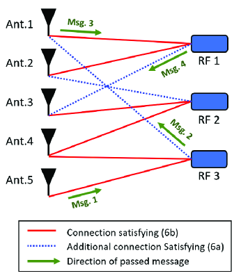
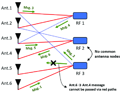
Figure 2: Example of the proposed LDPC-based structure for MP considering $\varrho=\text{mod}(N_{ant},N_{RF})$ with $N_{ant}\in\{5,6\}$ antenna nodes and $N_{RF}=3$ RF chain nodes. (a) $\varrho\neq 0$ and $N_{ant}=5$; (b) $\varrho=0$ and $N_{ant}=6$. Ant. and Msg. are acronyms for antenna and message, respectively.

To manage RF chains and antenna elements in the receiving BS, we consider that the HBF architecture is divided into several distributed virtual controllers as RF and antenna controllers. That is, several RF chains and antennas are clustered and controlled by their corresponding controllers, which are depicted in Fig. 1. We use the term controller to refer to a virtual controller in the remaining content for simplicity. In the LDPC-based connected HBF architecture, we deploy $N_{RF}^{C}$ RF chain controllers as $\mathcal{R}^{\mathcal{C}}\in\{\mathcal{R}_{1},...,\mathcal{R}_{k},...,{\mathcal{R}}_{N_{RF}^{C}}\}$ and $N_{ant}^{C}$ antenna controllers as $\mathcal{A}^{\mathcal{C}}\in\{\mathcal{A}_{1},...,\mathcal{A}_{l},...,{\mathcal{A}}_{N_{ant}^{C}}\}$, where ${\mathcal{R}}_{k}$ and ${\mathcal{A}}_{l}$ denote the control units of the $k$-th RF chain controller and the $l$-th antenna controller, respectively. Without loss of generality, we assume that antennas and RF chains cannot be managed by more than one controller, i.e., ${\mathcal{R}}_{k}\cap{\mathcal{R}}_{k^{\prime}}\!=\!\emptyset,\forall k^{\prime}\!\neq\!k,$ and ${\mathcal{A}}_{l}\cap{\mathcal{A}}_{l^{\prime}}\!=\!\emptyset,\forall l^{\prime}\!\neq\!l$. We assume that RF controller $\mathcal{R}_{k}$ manages $N_{RF,k}$ RF chains and antenna controller ${\mathcal{A}}_{l}$ manages $N_{ant,l}$ antenna elements. Due to the designed partial HBF structure, each control unit obtains only partial knowledge from neighboring linked nodes and its own determination. Therefore, we define that the $k$-th RF chain controller possesses an RF decision set $\boldsymbol{\delta}_{\mathcal{R}_{k}}\!=\!\{\delta_{\mathcal{R}_{k},1},...,\delta_{\mathcal{R}_{k},N_{RF,k}}\}$ and an antenna decision set from the $l$-th connected antenna controller $\boldsymbol{\theta}_{\mathcal{R}_{k},l}\!=\!\{\theta_{\mathcal{R}_{k},l,1},...,\theta_{\mathcal{R}_{k},l,N_{ant,l}}\}$. Similarly, the $l$-th antenna controller has its own antenna decision set $\boldsymbol{\theta}_{\mathcal{A}_{l}}\!=\!\{\theta_{\mathcal{A}_{l},1},...,\theta_{\mathcal{A}_{l},N_{ant,l}}\}$ and RF selection decision set from the neighboring RF controller $k$, namely, $\boldsymbol{\delta}_{\mathcal{A}_{l},k}\!=\!\{\delta_{\mathcal{A}_{l},k,1},...,\delta_{\mathcal{A}_{l},k,N_{RF,k}}\}$. The policy subsets at each controller are included in the total sets of RF and antenna selections as $\{\boldsymbol{\delta}_{\mathcal{R}_{k}},\boldsymbol{\delta}_{\mathcal{A}_{l},k},\forall k,l\}\in\boldsymbol{\delta}$ and $\{\boldsymbol{\theta}_{\mathcal{A}_{l}},\boldsymbol{\theta}_{\mathcal{R}_{k},l},\forall k,l\}\in\boldsymbol{\theta}$, respectively.

1:  Initialization: $\mathcal{A}$, $\mathcal{R}$, $N_{Conn}$ 2:  (Independent Connection Establishment) 3:  A temporary non-established connection set is selected as $\mathcal{M}=\mathcal{A}$ 4:  for $n=1,...,N_{RF}$ do 5:     A subset $\mathcal{M}^{\prime}$ with $\left\lceil\frac{N_{ant}}{N_{RF}}\right\rceil$ elements from $\mathcal{M}$ is randomly selected 6:     A binary vector indexed by subset $\mathcal{M}^{\prime}$ is generated based on $\eqref{LDPC1}$, i.e., we have $[\mathbf{C}]_{nm}=1$ for $m\in\mathcal{M}^{\prime}$ with the remaining elements being zero for $m\notin\mathcal{M}^{\prime}$ 7:     The non-established connection set is updated as $\mathcal{M}\leftarrow\mathcal{M}-\mathcal{M}^{\prime}$ 8:  end for 9:  (Node Dependency Construction) 10:  An initial pairing RF candidate $n\in\mathcal{R}$ is randomly selected 11:  A temporary non-selected RF set is selected as $\mathcal{N}=\mathcal{R}\backslash\{n\}$ 12:  for $iter=1,...,N_{RF}-1$ do 13:     A pairing RF $n^{\prime}\in\mathcal{N}\backslash\{n\}$ is randomly selected 14:     A common antenna node $m$ with $\mathbf{C}_{n^{\prime}m}=1$ is chosen, and $\mathbf{C}_{nm}=1$ is set 15:     The non-selected RF set is updated as $\mathcal{N}\leftarrow\mathcal{N}\backslash\{n^{\prime}\}$ and $n=n^{\prime}$ 16:  end for

Algorithm 1 LDPC-based HBF connection

IV Proposed Message Passing Antenna and RF Chain Selection (MARS) Scheme

Due to its high computational complexity, the original problem in (5) is decomposed into two subproblems, i.e., RF chain selection and antenna selection, which are determined by RF and antenna controllers, respectively. Each controller obtains its own solution according to the messages passed from other controllers, which can potentially reduce the system complexity. The subproblem of RF selection for the $k$-th RF chain controller is written as

$$\min_{\boldsymbol{\delta}_{\mathcal{R}_{k}}}\quad P\left(\boldsymbol{\delta}_{\mathcal{R}_{k}}\right)$$ (7a)

$$\text{s.t.}\quad\mbox{Fixed }\boldsymbol{\theta}_{\mathcal{R}_{k},l},\boldsymbol{\delta}_{\mathcal{R}_{k^{\prime}}},\forall l,k^{\prime}\not\neq k,$$ (7b)

$$\quad\quad\eqref{RF_blim},\eqref{RF_numlim},\eqref{SR_req},\eqref{P_lim},$$ (7c)

where $\eqref{RFp1}$ indicates the power consumption of the $k$-th RF chain given by the passed information of $\boldsymbol{\theta}_{\mathcal{R}_{k},l}$ from the $l$-th antenna controller and the message of $\boldsymbol{\delta}_{\mathcal{R}_{k^{\prime}}}$ from the neighboring $(k^{\prime})$-th RF chain in $\eqref{fix1}$. Furthermore, the subproblem of antenna selection for the $l$-th RF chain controller is given by

$$\min_{\boldsymbol{\theta}_{\mathcal{A}_{l}}}\quad P\left(\boldsymbol{\theta}_{\mathcal{A}_{l}}\right)$$ (8a)

$$\text{s.t.}\quad\mbox{Fixed }\boldsymbol{\delta}_{\mathcal{A}_{l},k},\boldsymbol{\theta}_{\mathcal{A}_{l^{\prime}}},\forall k,l^{\prime}\neq l,$$ (8b)

$$\quad\quad\eqref{ant_blim},\eqref{RF_numlim},\eqref{SR_req},\eqref{P_lim},\eqref{RF_insertionloss},$$ (8c)

where $\eqref{antp1}$ represents the total power consumption of the $l$-th antenna controller given by the passed information of $\boldsymbol{\delta}_{\mathcal{A}_{l},k}$ from the $k$-th RF controller and the message of $\theta_{\mathcal{A}_{l^{\prime}}}$ from the neighboring $(l^{\prime})$-th antenna controller in $\eqref{fix2}$. To address the two subproblems of RF/antenna selection, we propose the MARS scheme to minimize the operational circuit power of antennas and RF chains of receiving hybrid beamformers. Two types of MARS schemes are designed with sequential and parallel message passing, denoted by MARS-S and MARS-P, respectively. MARS can be iteratively performed in either a centralized or distributed manner based on computational complexity and algorithm convergence considerations. In a centralized architecture, more RF/antenna nodes are managed by an RF/antenna controller than in a distributed system. In the following, we will elaborate the MARS schemes, MARS-S and MARS-P.

IV-A MARS-S for Sequential Message Passing

In the proposed sequential mechanism of MARS-S, the antenna/RF controller passes the determined solutions in a sequential manner. As a result, the controllers are guaranteed to acquire the latest information from their neighboring nodes. The overall procedure of MARS-S is shown in Fig. 3, including four processing steps, which are elaborated in the following.

IV-A1 Initialization

At the beginning, all RF chain and antenna controllers exchange the determined beamformer matrices of $\mathbf{W_{BB}}$ and $\mathbf{W_{RF}}$ and channel information $\mathbf{H}$ to compute the achievable rate via $\eqref{recvcapacity}$. Furthermore, all RF/antenna selection elements in $\boldsymbol{\delta}$ and $\boldsymbol{\theta}$ are randomly generated in $\{0,1\}$.

IV-A2 Update Based on Received Messages

Afterward, the RF/antenna controllers will update the latest information on RF/antenna selections based on the received messages from the neighboring controllers. According to $\eqref{RFp1}$, the update information of the $k$-th RF chain controller at the $t$-th update consists of the $(k^{\prime})$-th RF chain decision $\boldsymbol{\delta}_{\mathcal{R}_{k^{\prime}}},\forall k^{\prime}\neq k$ and the passed antenna selection $\boldsymbol{\theta}_{\mathcal{R}_{k},l},\forall l$ at the $(t-1)$-th iteration, which are given by

$$\boldsymbol{\delta}_{{\mathcal{R}}_{k^{\prime}}}^{(t)}\!=\! \bigvee_{\mathcal{A}_{l}\in\mathcal{C}_{\mathcal{R}_{k}}}\left[\Xi_{\mathcal{R}}\land\nu_{\mathcal{A}_{l}\rightarrow\mathcal{R}_{k}}\left(\boldsymbol{\delta}_{\mathcal{A}_{l},{k^{\prime}}}^{(t-1)}\right)\right]\land\left\{\neg\left[\bigvee_{\mathcal{A}_{l}\in\mathcal{C}_{\mathcal{R}_{k}}}\left(\Xi_{\mathcal{R}}\land\boldsymbol{\delta}_{\mathcal{R}_{k^{\prime}}}^{(t-1)}\right)\right]\right\},$$ (9a)

$$\boldsymbol{\theta}_{\mathcal{R}_{k},l}^{(t)}\!=\! \bigvee_{\mathcal{A}_{l}\in\mathcal{C}_{\mathcal{R}_{k}}}\left[\Xi_{\mathcal{R}}^{{}^{\prime}}\land\nu_{\mathcal{A}_{l}\rightarrow\mathcal{R}_{k}}\left(\boldsymbol{\theta}_{\mathcal{A}_{l}}^{(t-1)}\right)\right]\land\left\{\neg\left[\bigvee_{\mathcal{A}_{l}\in\mathcal{C}_{\mathcal{R}_{k}}}\left(\Xi_{\mathcal{R}}^{{}^{\prime}}\land\boldsymbol{\theta}_{\mathcal{R}_{k},l}^{(t-1)}\right)\right]\right\},$$ (9b)

where $\Xi_{\mathcal{R}}=\nu_{\mathcal{A}_{l}\rightarrow\mathcal{R}_{k}}\left(\boldsymbol{\delta}_{\mathcal{A}_{l},{k^{\prime}}}^{(t-1)}\right)\oplus\boldsymbol{\delta}_{\mathcal{R}_{k^{\prime}}}^{(t-1)}$ and $\Xi_{\mathcal{R}}^{{}^{\prime}}=\nu_{\mathcal{A}_{l}\rightarrow\mathcal{R}_{k}}\left(\boldsymbol{\theta}_{\mathcal{A}_{l}}^{(t-1)}\right)\oplus\boldsymbol{\theta}_{\mathcal{R}_{k},l}^{(t-1)}$. The connection set of the $k$-th RF controller linked to its antenna controllers is denoted by $\mathcal{C}_{\mathcal{R}_{k}}$. Furthermore, we define $\nu_{\mathcal{A}_{l}\rightarrow\mathcal{R}_{k}}(\cdot)$ as the message passing operation that directs the path from the $l$-th antenna controller to the $k$-th RF chain controller. Similarly, according to $\eqref{antp1}$, the message of the $l$-th antenna controller at the $t$-th update consists of the $(l^{\prime})$-th antenna selection $\boldsymbol{\theta}_{\mathcal{A}_{l^{\prime}}},\forall l^{\prime}\neq l$ and the passed RF policy $\boldsymbol{\delta}_{\mathcal{A}_{l},k},\forall k$ at the $(t-1)$-th iteration, which are obtained as

$$\boldsymbol{\theta}_{{\mathcal{A}}_{l^{\prime}}}^{(t)}\!=\! \bigvee_{\mathcal{R}_{k}\in\mathcal{C}_{\mathcal{A}_{l}}}\left[\Xi_{\mathcal{A}}\land\mu_{\mathcal{R}_{k}\rightarrow\mathcal{A}_{l}}\left(\boldsymbol{\theta}_{\mathcal{R}_{k},{l^{\prime}}}^{(t-1)}\right)\right]\land\left\{\neg\left[\bigvee_{\mathcal{R}_{k}\in\mathcal{C}_{\mathcal{A}_{l}}}\left(\Xi_{\mathcal{A}}\land\boldsymbol{\theta}_{\mathcal{A}_{l^{\prime}}}^{(t-1)}\right)\right]\right\},$$ (10a)

$$\boldsymbol{\delta}_{\mathcal{A}_{l},k}^{(t)}\!=\! \bigvee_{\mathcal{R}_{k}\in\mathcal{C}_{\mathcal{A}_{l}}}\left[\Xi_{\mathcal{A}}^{{}^{\prime}}\land\mu_{\mathcal{R}_{k}\rightarrow\mathcal{A}_{l}}\left(\boldsymbol{\delta}_{\mathcal{R}_{k}}^{(t-1)}\right)\right]\land\left\{\neg\left[\bigvee_{\mathcal{R}_{k}\in\mathcal{C}_{\mathcal{A}_{l}}}\left(\Xi_{\mathcal{A}}^{{}^{\prime}}\land\boldsymbol{\delta}_{\mathcal{A}_{l},k}^{(t-1)}\right)\right]\right\},$$ (10b)

where $\Xi_{\mathcal{A}}=\mu_{\mathcal{R}_{k}\rightarrow\mathcal{A}_{l}}\left(\boldsymbol{\theta}_{\mathcal{R}_{k},{l^{\prime}}}^{(t-1)}\right)\oplus\boldsymbol{\theta}_{\mathcal{A}_{l^{\prime}}}^{(t-1)}$ and $\Xi_{\mathcal{A}}^{{}^{\prime}}=\mu_{\mathcal{R}_{k}\rightarrow\mathcal{A}_{l}}\left(\boldsymbol{\delta}_{\mathcal{R}_{k}}^{(t-1)}\right)\oplus\boldsymbol{\delta}_{\mathcal{A}_{l},k}^{(t-1)}$. The notation $\mathcal{C}_{\mathcal{A}_{l}}$ indicates the connection set of the $l$-th antenna controller associated with its RF controllers. Moreover, $\mu_{\mathcal{R}_{k}\rightarrow\mathcal{A}_{l}}(\cdot)$ is defined as the message passing operation directing the path from the $k$-th RF controller to the $l$-th antenna controller. Benefiting from the MP mechanism, we observe from the update equations $\eqref{para_update_RF}$ and $\eqref{para_update_antenna}$ that the RF/antenna controllers can readily update all information of the other RF/antenna nodes via simple logic operations to obtain their optimal solution for RF/antenna selections.

IV-A3 Optimization

Based on $\eqref{para_update_RF}$ and $\eqref{para_update_antenna}$, the RF/antenna controllers solve the decomposed subproblems in $\eqref{RFprob1}$ and $\eqref{antprob1}$ to obtain the optimum RF chain and antenna selections, which are given by

$$\boldsymbol{\delta}_{\mathcal{R}_{k}}^{*}={\arg\!\min}_{\boldsymbol{\delta}_{\mathcal{R}_{k}}}P\left(\boldsymbol{\delta}_{\mathcal{R}_{k}}\right)\mbox{ with fixed }\boldsymbol{\theta}_{\mathcal{R}_{k},l},\boldsymbol{\delta}_{\mathcal{R}_{k^{\prime}}},\forall l,k^{\prime}\not\neq k,$$ (11)

and

$$\boldsymbol{\theta}_{\mathcal{A}_{l}}^{*}={\arg\!\min}_{\boldsymbol{\theta}_{\mathcal{A}_{l}}}P\left(\boldsymbol{\theta}_{\mathcal{A}_{l}}\right)\mbox{ with fixed }\boldsymbol{\delta}_{\mathcal{A}_{l},k},\boldsymbol{\theta}_{\mathcal{A}_{l^{\prime}}},\forall k,l^{\prime}\neq l,$$ (12)

respectively. All RF and antenna constraints should be obeyed in $\eqref{conrf}$ and $\eqref{conant}$, respectively. Due to the partial connection of the LDPC-based HBF architecture, each controller is capable of managing a small number of nodes, which can achieve a much lower complexity. Accordingly, we can readily employ a numerical brute-force method to obtain the optimal binary-based parameters, i.e., we can search all possible solutions for a group of nodes given the information passed from others. Therefore, each RF/antenna controller can obtain its respective optimal solutions for RF selection in $\eqref{optrf}$ and antenna selection in $\eqref{optant}$.

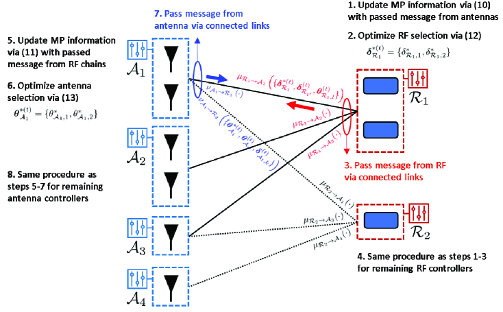
Figure 3: Example of sequential MP with the proposed MARS-S scheme considering $N_{ant}^{C}=4$ antenna controllers and $N_{RF}^{C}=2$ RF chain controllers.

IV-A4 Sequential Message Passing

After obtaining the optimal outcome of RF/antenna selection, the first controller passes its latest information to the neighboring connected nodes based on the LDPC-based HBF architecture. Then, the second controller managing its RF chains or antennas determines its own solution based on the information received from the neighboring controllers. That is, only one controller conducts MP while the others wait for the completion of message transfer. Therefore, the $k$-th RF controller employs the MP operation $\mu_{\mathcal{R}_{k}\rightarrow\mathcal{A}_{l}}\left(\{\boldsymbol{\delta}_{\mathcal{R}_{k}}^{*(t)},\boldsymbol{\delta}_{{\mathcal{R}}_{k^{\prime}}}^{(t)},\boldsymbol{\theta}_{\mathcal{R}_{k},l}^{(t)}\}\right)$ to pass its optimal RF selection $\boldsymbol{\delta}_{\mathcal{R}_{k}}^{*(t)}$ at the $t$-th iteration along with the updated information given in $\eqref{para_update_RF}$. Similarly, the $l$-th antenna controller transfers the optimal antenna selection and update information using $\nu_{\mathcal{A}_{l}\rightarrow\mathcal{R}_{k}}\left(\{\boldsymbol{\theta}_{\mathcal{A}_{l}}^{*(t)},\boldsymbol{\theta}_{{\mathcal{A}}_{l^{\prime}}}^{(t)},\boldsymbol{\delta}_{\mathcal{A}_{l},k}^{(t)}\}\right)$.

The concrete scheme of the proposed MARS-S as a sequential MP is described in Algorithm 2, which is also depicted in Fig. 3. All parameters are initialized randomly along with the measured channel information. First, the RF chain controller updates its decision according to the received message based on $\eqref{para_update_RF}$. We consider a randomized update method to prevent obtaining a locally optimal solution, i.e., $\eqref{optrf}$ is optimized when $x\leq\eta_{r}$, where $x$ is a random variable between $\left[0,1\right]$ and $\eta_{r}$ is a predefined learning rate. After obtaining the temporary optimal RF selection $\boldsymbol{\delta}_{\mathcal{R}_{k}}^{*(t)}$ constrained by $\eqref{conrf}$, the $k$-th RF chain controller passes the decision to the neighboring antenna controllers and updates the set $\{\boldsymbol{\delta}_{\mathcal{R}_{k}}^{*(t)},\boldsymbol{\delta}_{{\mathcal{R}}_{k^{\prime}}}^{(t)},\boldsymbol{\theta}_{\mathcal{R}_{k},l}^{(t)}\}$. The antenna controllers can perform their operations until the RF controllers have finished. Afterward, the antenna controllers adopt a process similar to that of the RF chain controllers to update, optimize, and pass messages. The update of antennas is based on $\eqref{para_update_antenna}$, while the optimization follows $\eqref{optant}$ constrained by $\eqref{conant}$. The optimal solution can be acquired if the random value $x$ is smaller than the given learning rate $\eta_{a}$ for antenna selection. Then, the $l$-th antenna controller transfers the decision to the connected RF controllers and updates the set $\{\boldsymbol{\theta}_{\mathcal{A}_{l}}^{*(t)},\boldsymbol{\theta}_{{\mathcal{A}}_{l^{\prime}}}^{(t)},\boldsymbol{\delta}_{\mathcal{A}_{l},k}^{(t)}\}$. Convergence occurs when the difference in power consumption between two iterations is smaller than a given threshold, i.e., $|P(\boldsymbol{\delta}^{(t-1)},\boldsymbol{\theta}^{(t-1)})-P(\boldsymbol{\delta}^{(t)},\boldsymbol{\theta}^{(t)})|\leq\kappa$.

1:  Initialization: $\mathbf{W_{BB}},\mathbf{W_{RF}},\mathbf{H},\mathbf{C},\boldsymbol{\delta},\boldsymbol{\theta},\eta_{r},\eta_{a},\kappa,t=1$ 2:  Channel estimation is performed to obtain $\mathbf{H}$ 3:  The beamformers $\mathbf{W_{BB}},\mathbf{W_{RF}}$ are randomized 4:  An LDPC-based connection is obtained based on Algorithm 1 5:  The BS broadcasts the above information to each controller 6:  repeat 7:     (RF Chain Controller) 8:     for $\mathcal{R}_{k}\in\mathcal{R}^{\mathcal{C}}$ do 9:        The $k$-th RF controller’s information is updated based on $\eqref{para_update_RF}$ 10:        A number $x\in[0,1]$ is randomly generated 11:        if $x\leq\eta_{r}$ then 12:           The temporary optimized RF chain selection $\boldsymbol{\delta}_{\mathcal{R}_{k}}^{*(t)}$ is obtained according to $\eqref{optrf}$ 13:           RF chains are reselected if $\eqref{conrf}$ is not satisfied 14:        end if 15:        The updated and optimized message is passed to neighboring connected controllers as $\mu_{\mathcal{R}_{k}\rightarrow\mathcal{A}_{l}}\left(\{\boldsymbol{\delta}_{\mathcal{R}_{k}}^{*(t)},\boldsymbol{\delta}_{{\mathcal{R}}_{k^{\prime}}}^{(t)},\boldsymbol{\delta}_{\mathcal{A}_{l},k}^{(t)}\}\right)$ 16:     end for 17:     (Antenna Controller) 18:     for $\mathcal{A}_{l}\in\mathcal{A}^{\mathcal{C}}$ do 19:        The $l$-th antenna controller’s information is updated according to $\eqref{para_update_antenna}$ 20:        A random number $x\in[0,1]$ is generated 21:        if $x\leq\eta_{a}$ then 22:           The temporary optimized antenna selection $\boldsymbol{\theta}_{\mathcal{A}_{l}}^{*(t)}$ is derived according to $\eqref{optant}$ 23:           If $\eqref{conant}$ is not satisfied, antennas are reselected 24:        end if 25:        The updated and optimized message is passed to neighboring connected controllers as $\nu_{\mathcal{A}_{l}\rightarrow\mathcal{R}_{k}}\left(\{\boldsymbol{\theta}_{\mathcal{A}_{l}}^{*(t)},\boldsymbol{\theta}_{{\mathcal{A}}_{l^{\prime}}}^{(t)},\boldsymbol{\delta}_{\mathcal{A}_{l},k}^{(t)}\}\right)$ 26:     end for 27:     (Optimum Derivation) 28:     The optimum of RF/antenna selection is $\{\boldsymbol{\delta}^{*},\boldsymbol{\theta}^{*}\}=\{\boldsymbol{\delta}^{(t)},\boldsymbol{\theta}^{(t)}\}$ 29:     Iteration update $t=t+1$ 30:  until Convergence of $|P(\boldsymbol{\delta}^{(t-1)},\boldsymbol{\theta}^{(t-1)})-P(\boldsymbol{\delta}^{(t)},\boldsymbol{\theta}^{(t)})|\leq\kappa$

Algorithm 2 Proposed MARS-S Scheme

IV-B MARS-P for Parallel Message Passing

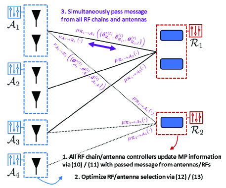
Figure 4: Example of parallel MP with the proposed MARS-P scheme considering $N_{ant}^{C}=4$ antenna controllers and $N_{RF}^{C}=2$ RF chain controllers.

1:  Initialization: $\mathbf{W_{BB}},\mathbf{W_{RF}},\mathbf{H},\mathbf{C},\boldsymbol{\delta},\boldsymbol{\theta},\eta_{r},\eta_{a},\kappa,t=1$ 2:  Channel estimation is performed to obtain $\mathbf{H}$ 3:  The beamformers $\mathbf{W_{BB}},\mathbf{W_{RF}}$ are randomized 4:  An LDPC-based connection is obtained based on Algorithm 1 5:  The BS broadcasts the above information to each controller 6:  repeat 7:     (RF Chain Controller) 8:     All RF controllers $\mathcal{R}_{k}\in\mathcal{R}^{\mathcal{C}}$ update their information according to $\eqref{para_update_RF}$ 9:     A temporary optimized RF chain selection $\boldsymbol{\delta}_{\mathcal{R}_{k}}^{*(t)}$ is acquired according to $\eqref{optrf}$ when the generated number of $x\in[0,1]$ is smaller than $\eta_{r}$ 10:     RF chains are reselected if $\eqref{conrf}$ is not satisfied 11:     (Antenna Controller) 12:     All antenna controllers $\mathcal{A}_{l}\in\mathcal{A}^{\mathcal{C}}$ update their information based on $\eqref{para_update_antenna}$ 13:     A temporary optimized antenna selection result is acquired $\boldsymbol{\delta}_{\mathcal{A}_{l}}^{*(t)}$ in $\eqref{optrf}$ when the generated number $x\in[0,1]$ is smaller than $\eta_{a}$ 14:     Antennas are reselected if $\eqref{conant}$ is not satisfied 15:     (Simultaneous Message Passing) 16:     All RF/antenna controllers simultaneously transfer the decision and latest message to the connected antenna/RF controllers by MP: $\mu_{\mathcal{R}_{k}\rightarrow\mathcal{A}_{l}}\left(\{\boldsymbol{\delta}_{\mathcal{R}_{k}}^{*(t)},\boldsymbol{\delta}_{{\mathcal{R}}_{k^{\prime}}}^{(t)},\boldsymbol{\delta}_{\mathcal{A}_{l},k}^{(t)}\}\right)$ and $\nu_{\mathcal{A}_{l}\rightarrow\mathcal{R}_{k}}\left(\{\boldsymbol{\theta}_{\mathcal{A}_{l}}^{*(t)},\boldsymbol{\theta}_{{\mathcal{A}}_{l^{\prime}}}^{(t)},\boldsymbol{\delta}_{\mathcal{A}_{l},k}^{(t)}\}\right),\forall\mathcal{R}_{k}\in\mathcal{R}^{\mathcal{C}},\forall\mathcal{A}_{l}\in\mathcal{A}^{\mathcal{C}}$ 17:     (Optimum Derivation) 18:     The optimum of RF/antenna selection is $\{\boldsymbol{\delta}^{*},\boldsymbol{\theta}^{*}\}=\{\boldsymbol{\delta}^{(t)},\boldsymbol{\theta}^{(t)}\}$ 19:     Iteration update $t=t+1$ 20:  until Convergence of $|P(\boldsymbol{\delta}^{(t-1)},\boldsymbol{\theta}^{(t-1)})-P(\boldsymbol{\delta}^{(t)},\boldsymbol{\theta}^{(t)})|\leq\kappa$

Algorithm 3 Proposed MARS-P Scheme

We can infer from MARS-S that it potentially induces a low convergence speed due to the sequential operation of MP. The adjacent controllers should wait until the completion of their connected controllers. Therefore, we design a parallel MP type, MARS-P, so that all RF/antenna controllers can simultaneously pass their optimized determinations. The steps of the proposed MARS-P scheme are similar to those of MARS-S for initialization, updating of $\eqref{para_update_RF}$ and $\eqref{para_update_antenna}$, and optimization of $\eqref{optrf}$ and $\eqref{optant}$ for RF and antenna selection, respectively. The only difference between MARS-P and MARS-S is the way in which parallel MP conveys information. The detailed algorithm of MARS-P is presented as Algorithm 3, which enables all controllers to simultaneously transmit messages without waiting. An example to demonstrate the process of MARS-P is illustrated in Fig. 4. However, due to the simultaneous update in MARS-P, each controller potentially suffers from local decisions, leading to a low convergence rate. Therefore, similar to MARS-S, we also need to design a feasible learning rate parameter to strike a compelling tradeoff between convergence and local optimality.

To elaborate a little further, the proposed MARS scheme can be used in both narrowband and wideband systems. There are two ways to modify the MARS algorithms for these systems. The first method is through an averaging approach, which involves estimating the wideband channel state information using a single parameter with the dimension of the multiplied numbers of transmitters and receivers. However, this approach results in lower complexity but worse performance due to the coarse channel estimation compared to fine-grained subchannel optimization. The second scheme is from a subchannel-based perspective, which provides better performance but is more complicated due to the coupled total power among subchannels. This may result in a trade-off among different subchannels, where selecting a certain subchannel may be harmful to another. To address this issue, an alternative optimization approach can be designed by adding an additional iteration loop to iteratively search over each subchannel until convergence. This approach enables us to apply the existing MARS algorithm directly in a wideband scenario, but it may require additional computational complexity depending on the number of subchannels being operated. Moreover, advanced beamforming can be designed to further enhance the system performance, whereas this work can be regarded as a lower bound of joint optimization of both RF/antenna selection and beamformer design, which will require additional complex mechanisms in the future.

IV-C Complexity Analysis

The computational complexity is demonstrated in Table II. We know that the joint solution for the conventional full-connection HBF architecture in problem $\eqref{mainprob}$ requires an exponential complexity of $\mathcal{O}\left(2^{N_{RF}N_{ant}}\right)$, which leads to a potential difficulty in acquiring the global optimum. On the other hand, the proposed MARS scheme possesses a much lower computational complexity than the exhaustive search of the original problem, i.e., MARS-S as a sequential MP scheme achieves a complexity of $\mathcal{O}\left(2^{|\mathcal{R}^{\mathcal{C}}|N_{RF,k}+|\mathcal{A}^{\mathcal{C}}|N_{ant,l}}\right)$, whereas the parallel-type mechanism of MARS-P possesses a complexity of $\mathcal{O}\left(2^{N_{RF,k}+N_{ant,l}}\right)$. It is observed that MARS-S has a higher computational complexity than MARS-P due to the sequential MP mechanism. The RF/antenna controllers update their latest information and then determine the corresponding selection results, which leads to no missed messages. In contrast, greedy-based selection [46] only considers a single-antenna policy with others fixed, which has a complexity order of $\mathcal{O}\left(|\mathcal{R}^{\mathcal{C}}|N_{RF,k}+|\mathcal{A}^{\mathcal{C}}|N_{ant,l}\right)$. Moreover, the genetic-based selection method [47], which adopts genetic generation, elite selection, crossover and mutation, possesses a complexity order of $\mathcal{O}\left(N_{crx}N_{RF}N_{ant}+N_{mu}\right)$, where $N_{crx}$ and $N_{mu}$ denote the numbers of crossover and mutation operations, respectively. Since both papers [46, 47] only consider antenna selection, we therefore adjust the genetic and greedy selection to also consider the RF selection problem for fair comparison. Due to the simultaneous passing of information in MARS-P, there may be either missed or out-of-date information, potentially resulting in a locally optimal solution. However, compared to the full connection of the HBF scheme in the original problem, the proposed MARS scheme reaches the lowest computational complexity while realizing nearly optimal solution acquisition.

TABLE II: Computational Complexity

Algorithm	Complexity
Global Optimum	$\mathcal{O}\left(2^{N_{RF}N_{ant}}\right)$
Proposed MARS-S	$\mathcal{O}\left(2^{|\mathcal{R}^{\mathcal{C}}|N_{RF,k}+|\mathcal{A}^{\mathcal{C}}|N_{ant,l}}\right)$
Proposed MARS-P	$\mathcal{O}\left(2^{N_{RF,k}+N_{ant,l}}\right)$
Greedy-Based Selection	$\mathcal{O}\left(|\mathcal{R}^{\mathcal{C}}|N_{RF,k}+|\mathcal{A}^{\mathcal{C}}|N_{ant,l}\right)$
Genetic-Based Selection	$\mathcal{O}\left(N_{crx}N_{RF}N_{ant}+N_{mu}\right)$

TABLE III: System Parameter Settings

Parameter	Value
Carrier frequency $f_{c}$	$28$ GHz
Distance between transmitter and receiver $d$	$100$ meters
Number of data stream $N_{S}$	$4$
Transmit power $P_{T}$ of user	$20$ dBm
Noise power $N_{0}$	$-85$ dBm
BS power consumption of an RF chain $P_{RF}$	$40$ mWatt
BS power consumption of baseband processing $P_{BB}$	$800$ mWatt
BS power consumption of an ADC $P_{ADC}$	$100$ mWatt
BS power consumption of a phase shifter $P_{PS}$	$10$ mWatt
BS power consumption of an LNA $P_{LNA}$	$10$ mWatt
Maximum output power for BS antennas $P_{o}$	$25$ dBm
Maximum allowable BS operating power $P_{max}$	$44$ dBm
Thresholds for RF and antenna selection $\eta_{r},\eta_{a}$	$0.7,0.7$

V Performance Evaluation

The performance of the proposed MARS scheme is evaluated via simulations. We consider a uplink transmission with a single transmitter and a hybrid beamformed-MIMO receiver. The distance between the transmitter and receiver is set to $d=100$ meters, and the operating carrier frequency is $f_{c}=28$ GHz. The transmit power of the user is set to $20$ dBm [48]. The receiver power consumption values of the BS utilized in our simulation are $P_{RF}=40$ mWatt, $P_{BB}=800$ mWatt, $P_{ADC}=100$ mWatt, and $P_{PS}=P_{LNA}=10$ mWatt [49, 50, 51, 52]. The maximum output power for the insertion loss of receiver antenna is $P_{o}=25$ dBm, and the allowable system operating power at receiving BS is $P_{max}=44$ dBm. The parameter $\rho=10^{-PL/10}$ refers to the distance-based path loss, where $PL=32.4+20\log_{10}(f_{c})+30\log_{10}(d)$ [53]. The learning rate threshold for RF/antenna selection is $\eta_{r}=\eta_{a}=0.7$. For simulation simplicity, we consider equivalent numbers of elements in each RF/antenna group, i.e., $N_{RF,k}=N_{RF}^{G}$ and $N_{ant,l}=N_{ant}^{G},\forall k,l$. The related outcome is characterized by power consumption (W) and corresponding EE (bits/J/Hz)^V , i.e., $EE=R(\mathbf{\Delta,\Theta})/P(\boldsymbol{\delta},\boldsymbol{\theta})$. The pertinent system parameters are listed in Table III.

V-A Convergence and Learning Rate

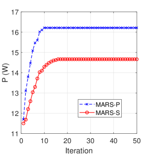
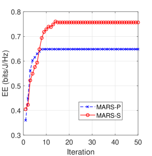
Figure 5: Convergence of the proposed MARS-S and MARS-P subschemes in terms of (a) power consumption and (b) EE.

As illustrated in Fig. 5, the convergence of the proposed MARS scheme is validated through simulations. We infer from both figures that the proposed MARS-S achieves lower power consumption and higher EE than MARS-P. This is because with sequential passing, up-to-date decisions can be completely conveyed to other nodes in order, whereas the parallel scheme potentially confuses RF/antenna controllers with multiple simultaneous received information. This results in worse information updates and corresponding low-performance policies. Moreover, because a better policy can be obtained from MARS-S, it requires more iterations to reach convergence. That is, MARS-S needs approximately $18$ iterations for the power consumption of approximately $14.7$ W and EE of $0.76$ bits/J/Hz, while MARS-P converges with a higher power consumption and lower EE at the $10$-th round, which strikes a compelling tradeoff between convergence speed and performance.

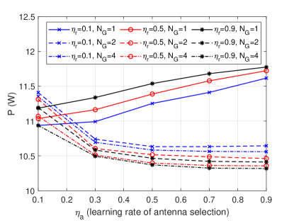
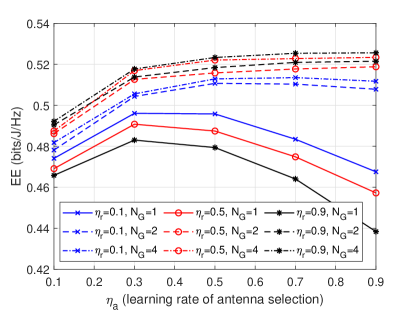
Figure 6: Performance of the proposed MARS scheme considering different learning rates for antenna selection $\eta_{a}\in\{0.1,0.3,0.5,0.7,0.9\}$ and RF selection $\eta_{r}\in\{0.1,0.5,0.9\}$ with $N_{G}=N_{RF}^{G}=N_{ant}^{F}\in\{1,2,4\}$ elements in each RF/antenna group with respect to (a) power consumption and (b) EE.

In Fig. 6, we evaluate the performance in terms of power consumption and EE of the proposed MARS scheme under different learning rates $\eta_{a}\in\{0.1,0.3,0.5,0.7,0.9\}$ for antenna selection and $\eta_{r}\in\{0.1,0.5,0.9\}$ for RF chain selection. We consider the same number of RF/antenna elements per group, $N^{G}=N_{RF}^{G}=N_{ant}^{G}\in\{1,4\}$. We observe from Figs. 6 and 6 that higher learning rates result in lower power consumption and higher EE when more nodes are managed by RF/antenna controllers, i.e., $N_{G}\in\{2,4\}$. This is because a quicker policy update can prevent out-of-date information from being conveyed to other controllers under a more centralized architecture, which requires fewer hops to convey the decision policy. However, under a more distributed architecture with fewer nodes per group, namely, $N_{G}=1$, a faster rate of $\eta_{a}=0.9$ consumes more power, up to an average of $11.7$ W, since the latest optimal message cannot be transferred to faraway nodes before the next update. The best policy is potentially obscured by newly passed messages from neighboring controllers. Moreover, concave EE curves are obtained for $N_{G}=1$ due to the moderate update speed, where the optimum is attained when $\eta_{a}=0.3$, as shown in Fig. 6.

V-B Different RF/Antenna Configurations

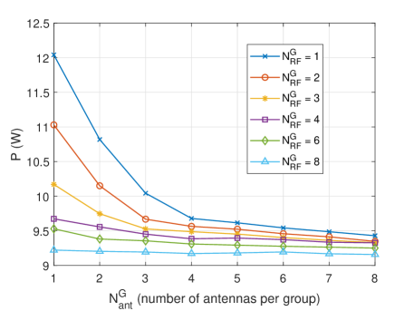
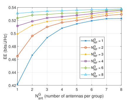
Figure 7: Performance of MARS with various numbers of clustered RF/antenna elements in groups $N_{RF}^{G}\in\{1,2,3,4,6,8\}$ and $N_{ant}^{G}\in\{1,2,3,4,5,6,7,8\}$, respectively, in terms of (a) power consumption and (b) EE.

As shown in Fig. 7, we evaluate the effects of different numbers of RF/antenna elements in each clustered group. We observe from Fig. 7 that a more centralized architecture with more antennas per group with larger $N_{ant}^{G}$ achieves lower power consumption when $N_{ant}^{G}\in\{1,2,3\}$. The first reason for this phenomenon is that the controller is capable of obtaining a nearer-optimal solution with a higher degree of freedom in selecting an on-off policy. The other reason is the shorter paths for conveying the determined message from one group to the others, which reveals similar effects, as illustrated in Fig. 6. Furthermore, the curves for $N_{RF}^{G}\in\{4,6,8\}$ are flatter than those of $N_{ant}^{G}\in\{1,2,3\}$ since the selection of RF chains, with considerably higher power consumption, becomes more dominant than antenna selection. This also implies that fewer RF controllers are potentially able to provide a better policy with lower power consumption and, accordingly, higher EE performance.

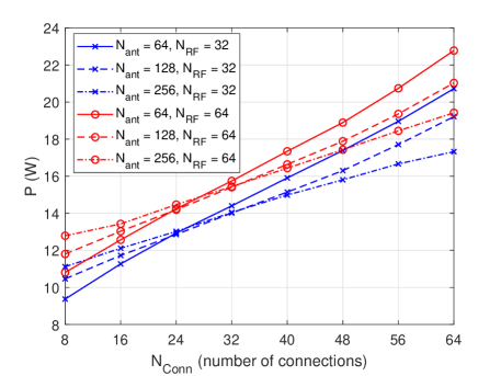
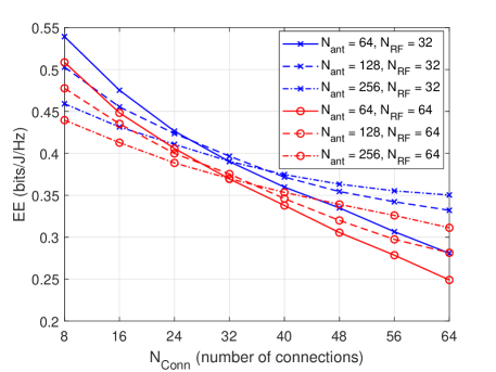
Figure 8: Effect of different numbers of connections $N_{conn}\in\{8,16,24,32,40,48,56,64\}$ with $N_{RF}\in\{32,64\}$ RF chains and $N_{ant}\in\{64,128,256\}$ antennas in terms of (a) power consumption and (b) EE.

In Fig. 8, we show the impact of the proposed MARS algorithm under different numbers of connections among RF/antenna controllers and nodes from $N_{Conn}=8$ to $64$ with $N_{RF}\in\{32,64\}$ RF chains and $N_{ant}\in\{64,128,256\}$ antennas. We recall that $N_{Conn}$ is the number of antennas associated with a single RF chain, which implies a tendency to become a fully connected beamformer. When $N_{Conn}=64$, it has the highest power consumption and lowest EE due to simultaneous message passing from nodes in different groups, which leads to more uncertain and complex decision-making. For example, an RF controller will update various distinct messages delivered from massive antenna groups connected to it, which may result in a more inappropriate update and corresponding local solution. Moreover, more antennas result in less power consumption due to a higher degree of freedom of selection, e.g., power reduces from $22.9$ W to $19.3$ W when $N_{ant}=64$ increases to $N_{ant}=256$ with $N_{RF}=64$ RF chains and $N_{Conn}=64$. However, RF selection exhibits reversed trend because it has higher operating power and lower selection freedom than antennas, which consumes approximately $2$ W power when $N_{RF}=64$ compared to the case of $N_{RF}=32$ under $N_{ant}=64$ antennas and $N_{Conn}=64$. To elaborate slightly further, we observe that another phenomenon takes place when we have the fewest connections, namely, $N_{Conn}\in\{8,16,24\}$. A higher number of antennas with fewer links can cause some optimal messages to be missed in the current iteration or confused with irrelevant information, deteriorating system performance.

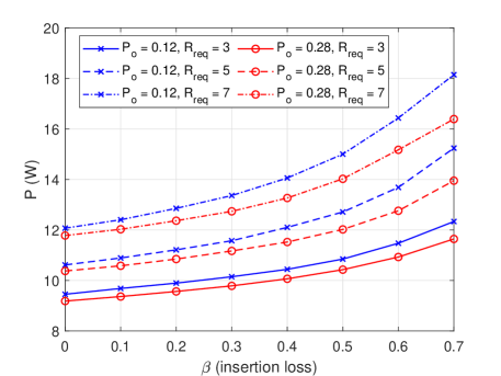
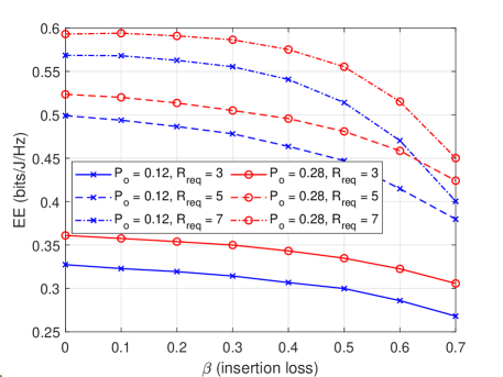
Figure 9: Performance of the proposed MARS scheme under different values of the insertion loss $\beta\in\{0,0.1,0.2,0.3,0.4,0.5,0.6,0.7\}$, maximum antenna output power $P_{o}\in\{0.12,0.28\}$ W, and QoS $R_{req}\in\{3,5,7\}$ bits/s/Hz in terms of (a) power consumption and (b) EE.

As depicted in Fig. 9, the performance of the proposed MARS algorithm is evaluated considering different values of the insertion loss and maximum antenna output power as well as QoS constraints. We observe from both the received signal in $\eqref{recvsignal}$ and throughput in $\eqref{recvcapacity}$ that both are monotonically decreasing and concave with respect to $\beta$. Thus, more power is consumed to compensate for the increased insertion loss, which exhibits a monotonically increasing convex shape, as shown in Fig. 9. Moreover, relaxed antenna output power restriction, i.e., $P_{o}=0.28$ W, requires lower power consumption due to the attainable higher degree of freedom in RF/antenna selection. Similarly, without any insertion loss, namely, when $\beta=0$, little difference in power consumption is observed due to the relaxed constraint in $\eqref{RF_insertionloss}$. Accordingly, most of the power can be utilized mainly for QoS satisfaction, not for compensation of insertion losses. With the increased rate demand, more power is intuitively required with a higher QoS requirement, e.g., we need approximately $4.4$ W more power in most cases when QoS increases from $3$ to $7$ bits/s/Hz. Moreover, as illustrated in Fig. 9, decreasing EE curves would intersect with $\beta$ larger than $0.6$ and QoS of $\{5,7\}$ bits/s/Hz because the system requires considerably higher power for QoS $R_{req}=7$ bits/s/Hz to simultaneously compensate for substantial insertion losses and satisfy the QoS requirement.

V-C Benchmarking

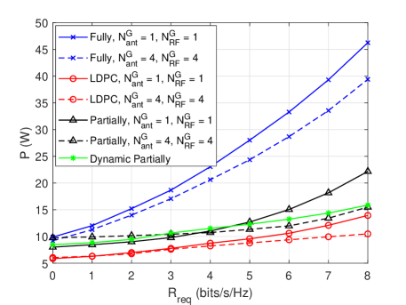
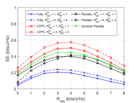
Figure 10: Performance comparison under different architectures of fully, partially, dynamic partially and LDPC-based connections with $N_{ant}^{G}=N_{RF}^{G}\in\{1,4\}$ RF/antenna elements per group and QoS requirements of $R_{req}\in\{0,1,2,3,4,5,6,7,8\}$ bits/s/Hz in terms of (a) power consumption and (b) EE. The dynamic partial connections are adjustable in each subarray size; hence, the parameters of $N_{ant}^{G}=N_{RF}^{G}$ are not set.

In Fig. 10, we compare the performance under different architectures, i.e., full connection [24, 25, 26], fixed partial connection [18, 54, 55], the dynamic partial connection designed in [23] and the proposed LDPC-based architecture considering different numbers of RF/antenna elements per group and QoS requirements. We also compare two different types of partial connections. Dynamic partial connection in [23] is performed by exhaustively obtaining the optimal subarray patterns, i.e., each subarray has different sizes of elements but is fully connected in its group with the same connection as in the fixed case. This potentially provides a higher degree of freedom to construct a high-EE partial connection, which accordingly achieves a higher EE with similar power consumption to the fixed partially connected architecture. Moreover, as explained previously, it requires more power to satisfy higher QoS demands, especially under the fully connected architecture with excessive power consumption up to approximately $47$ W. Partial connection results in approximately $5$ to $10$ W more power utilization than the proposed LDPC-based architecture since the controllers with partial connections cannot acquire certain messages passed from some nodes, leading to worse solutions. Furthermore, a larger difference in power is induced by higher QoS requirements by comparing the distributed control architecture with $N_{ant}^{G}=N_{RF}^{G}=1$ and a centralized architecture with $N_{ant}^{G}=N_{RF}^{G}=4$. This is because some information in the distributed architecture has to be conveyed from faraway nodes with massive hops, generating an out-of-date policy to fulfill high QoS requirements, as also shown in Fig. 7. To elaborate a little further, we observe opposite trends for the partially connected method. Under lower QoS $R_{req}\leq 4$ bits/s/Hz, controllers in a more distributed arrangement, i.e., $N_{ant}^{G}=N_{RF}^{G}=1$, tend to greedily optimize themselves due to unknown or nonupdated messages passed from others. In contrast, a more centralized arrangement with $N_{ant}^{G}=N_{RF}^{G}=4$ is able to provide a more appropriate policy with adequate QoS-aware information, achieving lower power and, accordingly, higher EE. In conclusion, the proposed LDPC-based architecture under the MARS scheme can conserve approximately $32$ W and $9$ W and achieves approximately triple and twice EE compared to fully and partially connected structures, respectively.

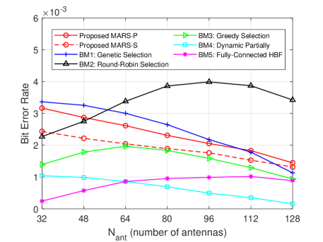
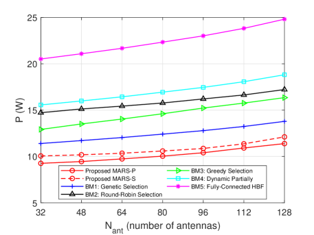
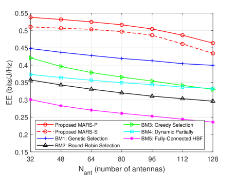
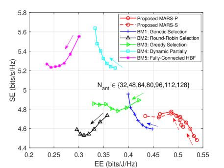
Figure 11: Performance comparison of the proposed MARS scheme and benchmarks of genetic-, greedy- and round robin-based selection with various numbers of receiving antennas $N_{ant}\in\{32,48,64,80,96,112,128\}$ in terms of (a) bit error rate, (b) power consumption, (c) EE, and (d) spectrum-energy efficiency. The direction of the arrows indicates the increment of $N_{ant}$.

In Fig. 11, we compare the comprehensive performance in terms of the bit error rate (BER), power consumption, EE, and spectrum-energy efficiency for the proposed MARS schemes MARS-P and MARS-S with five benchmarks (BMs), with are elaborated as follows. Note that modulation of 64-quadrature modulation (64-QAM) is adopted for computing BER. We consider an equivalent QoS constraint $R_{req}=3$ bits/s/Hz, insertion loss $\beta=0.3$, $N_{RF}=32$, and $N_{RF}^{G}=N_{ant}^{G}=4$ for a fair comparison.

• BM1 Genetic-Based Selection [47]: The selection solution is initially provided with a given genetic population size. The candidate solution is obtained by adopting a discrete genetic algorithm with crossover, mutation, elite selection and offspring gene generation. All RF chains are selected to operate, i.e., $\delta_{n}=1\ \forall n\in\mathcal{R}$. This case is conducted based on the designed LDPC-based connection.

• BM2 Round-Robin Selection: The candidate solution of RF/antenna selection is randomly initialized and evaluated in a round-robin manner. We change the mechanism in [56] from MIMO user scheduling to RF/antenna selection. The policy under fully off antennas or RF chains is excluded here due to zero rate performance. This case is conducted based on the designed LDPC-based connection.

• BM3 Greedy-Based Selection [46]: It optimizes the policy of a single antenna with the other solutions fixed, which can be regarded as a distributed approach with $N_{ant}^{G}=1$ in this work. First, we randomly conduct antenna selection by either turning on or off all nodes. Afterwards, we iteratively select the antenna that leads to the lowest power consumption in a selfish manner until the completion of the final node. All RF chains are selected to be under operation, i.e., $\delta_{n}=1\ \forall n\in\mathcal{R}$. This case is conducted based on the designed LDPC-based connection.

• BM4 Dynamic Partial Connection [23]: This connection is implemented by exhaustively obtaining the optimal subarray patterns, i.e., each subarray has elements of different sizes but is fully connected in its subgroup as in the fixed case, which provides a higher degree of freedom than partial connection with an equal subarray size. All RF chains and antennas in each subarray are selected to be operated.

• BM5 Fully Connected HBF [57]: The conventional HBF architecture is implemented under a full connection with whole RF chains and antennas selected to be operated.

In Fig. 11, we observe that BMs 4 and 5 have the lowest BERs due to there being more connected links in HBF, i.e., more information with a higher degree of freedom can be obtained to achieve a higher rate. BMs 1 and 3 show medium BER performance under the LDPC architecture. With similar performance, the proposed MARS scheme has a lower BER with more antennas due to more information being passed. Round robin potentially switches off beneficial nodes, leading to the worst BER. To elaborate a little further, BER reflects the negative correlation in the performance in terms of spectrum efficiency (SE), as shown in Fig. 11, i.e., a lower BER corresponds to a higher SE. We infer from Fig. 11 that more power is required to operate the increased number of deployed antennas. Considering the LDPC architecture, however, BM2 requires the highest power due to random selection without any information utilization. For BM3, a selfish-style method is employed to optimize its own antenna selection without using messages from other controller groups. However, as a compromise mechanism in BM1, genetic-based selection takes into account the selection policy from other groups, which preserves powers of $2.8$ W and $2$ W compared to round-robin and greedy selection, respectively, under $N_{ant}=128$. In contrast, BM4, regarded as the optimal solution with partial connection, requires slightly more power than the baseline solution in the LDPC architecture due to comparably fewer links being required to achieve satisfactory service. Moreover, BM5 with full connection consumes the most power resources, approximately twice as much as the proposed MARS schemes.

Although MARS-P has a faster policy update speed, it potentially leads to missed information due to the parallel transfer in message passing, which has a slightly higher power of approximately $0.5$ W compared to the sequential approach in MARS-S. Benefiting from both the LDPC connection and message passing-based design, the proposed MARS can exactly convey appropriate information to all the other controller groups to realize a better RF/antenna selection policy. In this context, as observed from Figs. 11 and 11 considering $N_{ant}=128$, the proposed MARS scheme outperforms all the benchmarks, which is able to preserve powers of approximately $2.4$, $5.8$, $5$, $7.43$ and $13.4$ W and to improve EE by approximately $9\%$, $47\%$, $32\%$, $31\%$ and $85\%$ compared to BMs 1 to 5, respectively. Furthermore, as shown in Fig. 11, it also strikes a tradeoff between the SE and EE metrics. MARS accomplishes the highest EE at the expense of moderate throughput, while full connection alternatively has the highest rate by consuming the most power, leading to the lowest EE. Additionally, BMs 1 and 4 exhibit asymptotic shaped curves because the optimal solution is potentially obtained from genetic selection with a smaller search space.

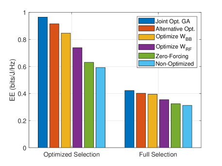
Figure 12: Comparison of different beamforming methods for $\mathbf{W_{BB}}$ and $\mathbf{W_{RF}}$ with $N_{ant}=64$ and $N_{RF}=32$.

At last, in Fig. 12 we compare different beamforming methods, including genetic-based algorithm, alternative optimization, and zero-forcing for providing appropriate beamformers of $\mathbf{W_{BB}}$ and $\mathbf{W_{RF}}$ with or without the optimized RF/antenna selection mechanism. The MARS-P is performed for the optimized selection, whilst full selection turns on all antennas and RF chains. Genetic-based algorithm provides the joint solution by considering both beamformers at the same time through the process of gene generation, elite selection crossover and mutation. In alternative optimization, the two parameters undergo rotational optimization, i.e., $\mathbf{W_{BB}}$ is optimized based on the optimal $\mathbf{W_{RF}}$ from previous iteration. Note that optimizing $\mathbf{W_{BB}}$ indicates the method only optimizes $\mathbf{W_{BB}}$ with random $\mathbf{W_{RF}}$. Same process takes place for $\mathbf{W_{RF}}$-only optimization. Random method is conducted for the non-optimized beamforming. In Fig. 12, we can readily observe that it has a lower EE due to high power consumption of full selection. Performance gain of additional beamforming can also be achieved, i.e., joint optimization has improved EE with approximately $5.3\%$, $14\%$, $30.6\%$, $52.9\%$, $62.8\%$ compared to alternative optimization, optimizing $\mathbf{W_{BB}}$/$\mathbf{W_{RF}}$-only, zero-forcing, non-optimized beamforming, respectively. This is because more power can be preserved upon satisfaction of rate requirement.

VI Conclusions

In this paper, we propose an LDPC-based HBF structure and MARS scheme to jointly consider RF chain and antenna selection for the minimization of operating power consumption, which guarantees QoS and available power utilization. MARS can be employed under sequential (MARS-S) and parallel (MARS-P) message passing under either a distributed or centralized architecture. The performance reveals that MARS-P has faster convergence than MARS-S due to parallel information delivery. However, MARS-S achieves lower power consumption and higher EE due to nonoverlapped decisions from fewer neighboring nodes. Additionally, missed messages or out-of-date policies are resolved by selecting appropriate learning rates for RF chains and antenna selections. Due to dominant RF chains, performance is more significantly influenced by RF chains than antennas under different numbers of controllers, connections, and hardware impairment effects. Moreover, the proposed LDPC-based structure with MARS achieves the lowest power and highest EE since it possesses considerably fewer links than the fully connected architecture but with more information exchanged than the partially connected architecture. Additionally, benefitting from better messages and policies being passed from other RF/antenna nodes, MARS outperforms various existing algorithms, namely, round-robin, greedy-based, and genetic-based selection methods, as well as dynamic adjustment of partial/full connection, in the open literature.

References

- [1] W. Saad, M. Bennis, and M. Chen, “A vision of 6G wireless systems: Applications, trends, technologies, and open research problems,” IEEE Network, vol. 34, no. 3, pp. 134–142, 2020.
- [2] L.-H. Shen, K.-T. Feng, and L. Hanzo, “Five facets of 6G: Research challenges and opportunities,” ACM Computing Surveys, vol. 55, no. 11, pp. 1–39, 2023.
- [3] H. Zhang, S. Huang, C. Jiang, K. Long, V. C. M. Leung, and H. V. Poor, “Energy efficient user association and power allocation in millimeter-wave-based ultra dense networks with energy harvesting base stations,” IEEE Journal on Selected Areas in Communications, vol. 35, no. 9, pp. 1936–1947, 2017.
- [4] T. Huang, W. Yang, J. Wu, J. Ma, X. Zhang, and D. Zhang, “A survey on green 6G network: Architecture and technologies,” IEEE Access, vol. 7, pp. 175 758–175 768, 2019.
- [5] S. Yang and L. Hanzo, “Fifty years of MIMO detection: The road to large-scale MIMOs,” IEEE Communications Surveys Tutorials, vol. 17, no. 4, pp. 1941–1988, 2015.
- [6] Q.-U.-A. Nadeem, A. Kammoun, and M.-S. Alouini, “Elevation beamforming with full dimension MIMO architectures in 5G systems: A tutorial,” IEEE Communications Surveys Tutorials, vol. 21, no. 4, pp. 3238–3273, 2019.
- [7] S. Kutty and D. Sen, “Beamforming for millimeter wave communications: An inclusive survey,” IEEE Communications Surveys Tutorials, vol. 18, no. 2, pp. 949–973, 2016.
- [8] S. Han, C.-l. I, Z. Xu, and C. Rowell, “Large-scale antenna systems with hybrid analog and digital beamforming for millimeter wave 5G,” IEEE Communications Magazine, vol. 53, no. 1, pp. 186–194, 2015.
- [9] S. S. Ioushua and Y. C. Eldar, “A family of hybrid analog–digital beamforming methods for massive MIMO systems,” IEEE Transactions on Signal Processing, vol. 67, no. 12, pp. 3243–3257, 2019.
- [10] I. Ahmed, H. Khammari, A. Shahid, A. Musa, K. S. Kim, E. De Poorter, and I. Moerman, “A survey on hybrid beamforming techniques in 5G: Architecture and system model perspectives,” IEEE Communications Surveys Tutorials, vol. 20, no. 4, pp. 3060–3097, 2018.
- [11] L.-H. Shen and K.-T. Feng, “Mobility-aware subband and beam resource allocation schemes for millimeter wave wireless networks,” IEEE Transactions on Vehicular Technology, vol. 69, no. 10, pp. 11 893–11 908, 2020.
- [12] Y. Cai, Y. Xu, Q. Shi, B. Champagne, and L. Hanzo, “Robust joint hybrid transceiver design for millimeter wave full-duplex MIMO relay systems,” IEEE Transactions on Wireless Communications, vol. 18, no. 2, pp. 1199–1215, 2019.
- [13] L.-H. Shen, Y.-C. Chen, and K.-T. Feng, “Design and analysis of multi-user association and beam training schemes for millimeter wave based WLANs,” IEEE Transactions on Vehicular Technology, vol. 69, no. 7, pp. 7458–7472, 2020.
- [14] L.-H. Shen, K.-T. Feng, and L. Hanzo, “Coordinated multiple access point multiuser beamforming training protocol for millimeter wave WLANs,” IEEE Transactions on Vehicular Technology, vol. 69, no. 11, pp. 13 875–13 889, 2020.
- [15] L.-H. Shen, T.-W. Chang, K.-T. Feng, and P.-T. Huang, “Design and implementation for deep learning based adjustable beamforming training for millimeter wave communication systems,” IEEE Transactions on Vehicular Technology, vol. 70, no. 3, pp. 2413–2427, 2021.
- [16] H. Li, M. Li, Q. Liu, and A. L. Swindlehurst, “Dynamic hybrid beamforming with low-resolution PSs for wideband mmwave MIMO-OFDM systems,” IEEE Journal on Selected Areas in Communications, vol. 38, no. 9, pp. 2168–2181, 2020.
- [17] Y. Zhang, J. Du, Y. Chen, M. Han, and X. Li, “Optimal hybrid beamforming design for millimeter-wave massive multi-user MIMO relay systems,” IEEE Access, vol. 7, pp. 157 212–157 225, 2019.
- [18] Y. Zhang, J. Du, Y. Chen, X. Li, K. M. Rabie, and R. Khkrel, “Dual-iterative hybrid beamforming design for millimeter-wave massive multi-user MIMO systems with sub-connected structure,” IEEE Transactions on Vehicular Technology, vol. 69, no. 11, pp. 13 482–13 496, 2020.
- [19] H. Gao, D. Liu, and Z. Zhang, “Low-resolution DACs aided partially-connected hybrid precoding design for MU-MISO system,” IEEE Communications Letters, pp. 1–1, 2023.
- [20] X. Wang, Z. Fei, J. A. Zhang, and J. Xu, “Partially-connected hybrid beamforming design for integrated sensing and communication systems,” IEEE Transactions on Communications, vol. 70, no. 10, pp. 6648–6660, 2022.
- [21] A. Morsali, A. Haghighat, and B. Champagne, “Generalized framework for hybrid analog/digital signal processing in massive and ultra-massive-MIMO systems,” IEEE Access, vol. 8, pp. 100 262–100 279, 2020.
- [22] D. Zhang, Y. Wang, X. Li, and W. Xiang, “Hybridly connected structure for hybrid beamforming in mmwave massive MIMO systems,” IEEE Transactions on Communications, vol. 66, no. 2, pp. 662–674, 2018.
- [23] Y. Chen, D. Chen, T. Jiang, and L. Hanzo, “Millimeter-wave massive MIMO systems relying on generalized sub-array-connected hybrid precoding,” IEEE Transactions on Vehicular Technology, vol. 68, no. 9, pp. 8940–8950, 2019.
- [24] N. N. Moghadam, G. Fodor, M. Bengtsson, and D. J. Love, “On the energy efficiency of MIMO hybrid beamforming for millimeter-wave systems with nonlinear power amplifiers,” IEEE Transactions on Wireless Communications, vol. 17, no. 11, pp. 7208–7221, 2018.
- [25] M. Sefunç, A. Zappone, and E. A. Jorswieck, “Energy efficiency of mmwave MIMO systems with spatial modulation and hybrid beamforming,” IEEE Transactions on Green Communications and Networking, vol. 4, no. 1, pp. 95–108, 2020.
- [26] L. Zhao, M. Li, C. Liu, S. V. Hanly, I. B. Collings, and P. A. Whiting, “Energy efficient hybrid beamforming for multi-user millimeter wave communication with low-resolution A/D at transceivers,” IEEE Journal on Selected Areas in Communications, vol. 38, no. 9, pp. 2142–2155, 2020.
- [27] A. Kaushik, E. Vlachos, C. Tsinos, J. Thompson, and S. Chatzinotas, “Joint bit allocation and hybrid beamforming optimization for energy efficient millimeter wave MIMO systems,” IEEE Transactions on Green Communications and Networking, vol. 5, no. 1, pp. 119–132, 2021.
- [28] C. Qi, W. Ci, J. Zhang, and X. You, “Hybrid beamforming for millimeter wave MIMO integrated sensing and communications,” IEEE Communications Letters, vol. 26, no. 5, pp. 1136–1140, 2022.
- [29] X. Yu, L. Tu, Q. Yang, M. Yu, Z. Xiao, and Y. Zhu, “Hybrid beamforming in mmwave massive MIMO for IoV with dual-functional radar communication,” IEEE Transactions on Vehicular Technology, vol. 72, no. 7, pp. 9017–9030, 2023.
- [30] S. Payami, M. Ghoraishi, and M. Dianati, “Hybrid beamforming for large antenna arrays with phase shifter selection,” IEEE Transactions on Wireless Communications, vol. 15, no. 11, pp. 7258–7271, 2016.
- [31] A. Kaushik, J. Thompson, E. Vlachos, C. Tsinos, and S. Chatzinotas, “Dynamic RF chain selection for energy efficient and low complexity hybrid beamforming in millimeter wave MIMO systems,” IEEE Transactions on Green Communications and Networking, vol. 3, no. 4, pp. 886–900, 2019.
- [32] E. Vlachos and J. Thompson, “Energy-efficiency maximization of hybrid massive MIMO precoding with random-resolution DACs via RF selection,” IEEE Transactions on Wireless Communications, vol. 20, no. 2, pp. 1093–1104, 2021.
- [33] F. Kschischang, B. Frey, and H.-A. Loeliger, “Factor graphs and the sum-product algorithm,” IEEE Transactions on Information Theory, vol. 47, no. 2, pp. 498–519, 2001.
- [34] J. Zeng, J. Lin, and Z. Wang, “Low complexity message passing detection algorithm for large-scale MIMO systems,” IEEE Wireless Communications Letters, vol. 7, no. 5, pp. 708–711, 2018.
- [35] Z. Sui, S. Yan, H. Zhang, L.-L. Yang, and L. Hanzo, “Approximate message passing algorithms for low complexity OFDM-IM detection,” IEEE Transactions on Vehicular Technology, vol. 70, no. 9, pp. 9607–9612, 2021.
- [36] N. J. Myers, J. Kaleva, A. Tölli, and R. W. Heath, “Message passing-based link configuration in short range millimeter wave systems,” IEEE Transactions on Communications, vol. 68, no. 6, pp. 3465–3479, 2020.
- [37] Y. Jeong, C. Lee, and Y. H. Kim, “Power minimizing beamforming and power allocation for MISO-NOMA systems,” IEEE Transactions on Vehicular Technology, vol. 68, no. 6, pp. 6187–6191, 2019.
- [38] N.-I. Kim and D.-H. Cho, “Scheduling and layer selection based performance improvement of uplink SCMA system with receive beamforming,” IEEE Transactions on Vehicular Technology, vol. 68, no. 7, pp. 7209–7213, 2019.
- [39] Y. Yu, M. Pischella, and D. Le Ruyet, “Distributed antenna selection with message passing algorithm for MIMO D2D communications,” in Proc. IEEE International Symposium on Wireless Communication Systems (ISWCS), 2017, pp. 454–458.
- [40] R. Gallager, “Low-density parity-check codes,” IRE Transactions on Information Theory, vol. 8, no. 1, pp. 21–28, 1962.
- [41] T. Richardson, M. Shokrollahi, and R. Urbanke, “Design of capacity-approaching irregular low-density parity-check codes,” IEEE Transactions on Information Theory, vol. 47, no. 2, pp. 619–637, 2001.
- [42] O. Hiari and R. Mesleh, “Impact of RF–switch insertion loss on the performance of space modulation techniques,” IEEE Communications Letters, vol. 22, no. 5, pp. 958–961, 2018.
- [43] Z. Wang, X. Mu, J. Xu, and Y. Liu, “Simultaneously transmitting and reflecting surface (STARS) for terahertz communications,” IEEE Journal of Selected Topics in Signal Processing, pp. 1–16, 2023.
- [44] F. Bishe, A. Koc, and T. Le-Ngoc, “Intelligent subcarrier allocation in hybrid beamforming multi-user mMIMO-OFDM systems,” in Proc. IEEE Vehicular Technology Conference (VTC-Spring), 2023, pp. 1–5.
- [45] C. Zhang, W. Xu, and M. Chen, “Hybrid zero-forcing beamforming/orthogonal beamforming with user selection for MIMO broadcast channels,” IEEE Communications Letters, vol. 13, no. 1, pp. 10–12, 2009.
- [46] M. O. K. Mendonça, P. S. R. Diniz, T. N. Ferreira, and L. Lovisolo, “Antenna selection in massive MIMO based on greedy algorithms,” IEEE Transactions on Wireless Communications, vol. 19, no. 3, pp. 1868–1881, 2020.
- [47] J. C. Marinello, T. Abrão, A. Amiri, E. de Carvalho, and P. Popovski, “Antenna selection for improving energy efficiency in XL-MIMO systems,” IEEE Transactions on Vehicular Technology, vol. 69, no. 11, pp. 13 305–13 318, 2020.
- [48] J. Brun, V. Palhares, G. Marti, and C. Studer, “Beam alignment for the cell-free mmwave massive MU-MIMO uplink,” in Proc. IEEE Workshop on Signal Processing Systems (SiPS), 2022, pp. 1–6.
- [49] R. Méndez-Rial, C. Rusu, N. González-Prelcic, A. Alkhateeb, and R. W. Heath, “Hybrid MIMO architectures for millimeter wave communications: Phase shifters or switches?” IEEE Access, vol. 4, pp. 247–267, 2016.
- [50] H. Krishna, R. Rajakumar, and S. Chakrabarti, “Quantifying the improvement in energy savings for LTE enodeb baseband subsystem with technology scaling and multi-core architectures,” in Proc. National Conference on Communications (NCC), 2012, pp. 1–5.
- [51] M. Kadam, S. Aniruddhan, and A. Kumar, “An unconditionally stable 28 ghz 18 db gain LNA employing current-reuse,” in Proc. IEEE International Symposium on Circuits and Systems (ISCAS), 2020, pp. 1–4.
- [52] P. Skrimponis, S. Dutta, M. Mezzavilla, S. Rangan, S. H. Mirfarshbafan, C. Studer, J. Buckwalter, and M. Rodwell, “Power consumption analysis for mobile mmwave and sub-THz receivers,” in Proc. IEEE 6G Wireless Summit (6G SUMMIT), 2020, pp. 1–5.
- [53] 3GPP, “Study on channel model for frequencies from 0.5 to 100 GHz,” no. TR 38.901 version 16.1.0 Release 16, Nov. 2020.
- [54] X. Song, T. Kühne, and G. Caire, “Fully-/partially-connected hybrid beamforming architectures for mmwave MU-MIMO,” IEEE Transactions on Wireless Communications, vol. 19, no. 3, pp. 1754–1769, 2020.
- [55] N. T. Nguyen and K. Lee, “Unequally sub-connected architecture for hybrid beamforming in massive MIMO systems,” IEEE Transactions on Wireless Communications, vol. 19, no. 2, pp. 1127–1140, 2020.
- [56] H. A. Ammar, R. Adve, S. Shahbazpanahi, G. Boudreau, and K. V. Srinivas, “Downlink resource allocation in multiuser cell-free MIMO networks with user-centric clustering,” IEEE Transactions on Wireless Communications, vol. 21, no. 3, pp. 1482–1497, 2022.
- [57] B.-Y. Chen, Y.-F. Chen, and S.-M. Tseng, “Hybrid beamforming and data stream allocation algorithms for power minimization in multi-user massive MIMO-OFDM systems,” IEEE Access, vol. 10, pp. 101 898–101 912, 2022.