CASA: Category-agnostic Skeletal Animal Reconstruction

Abstract

Recovering the skeletal shape of an animal from a monocular video is a longstanding challenge. Prevailing animal reconstruction methods often adopt a control-point driven animation model and optimize bone transforms individually without considering skeletal topology, yielding unsatisfactory shape and articulation. In contrast, humans can easily infer the articulation structure of an unknown animal by associating it with a seen articulated character in their memory. Inspired by this fact, we present CASA, a novel Category-Agnostic Skeletal Animal reconstruction method consisting of two major components: a video-to-shape retrieval process and a neural inverse graphics framework. During inference, CASA first retrieves an articulated shape from a 3D character assets bank so that the input video scores highly with the rendered image, according to a pretrained language-vision model. CASA then integrates the retrieved character into an inverse graphics framework and jointly infers the shape deformation, skeleton structure, and skinning weights through optimization. Experiments validate the efficacy of CASA regarding shape reconstruction and articulation. We further demonstrate that the resulting skeletal-animated characters can be used for re-animation.

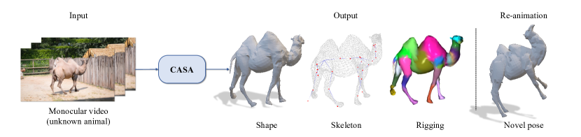
Figure 1: Given a monocular video with an animal from unknown category, CASA jointly infers the articulated skeletal shape and rigging through optimization, which can be animated into novel poses.

1 Introduction

Recovering the shape, articulation, and dynamics of animals from images and videos is a long-standing task in computer vision and graphics. Achieving this goal will enable numerous future applications for 3D modeling and reanimation of animals. Nevertheless, accurately reasoning about the geometry and kinematics of animals in the wild remains an ambitious problem for three reasons: 1) partial visibility of the captured animal, 2) variability of shape across different categories, and 3) ambiguity of unknown kinematics. Take the camel in Fig. 1 as an example – to faithfully model it requires: 1) hallucinating the unobserved (e.g., occluded, back-side) region, 2) recovering its unique shape and scale, and 3) predicting its kinematic structure.

Remarkable progress has been made in addressing the aforementioned challenges by either exploiting richer sensor configurations (e.g., multi-view cameras [11, 17] or depth sensors [41, 42, 50]), or by making strong class-specific assumptions (e.g., humans [34, 55, 56, 57, 78, 80] or quadruped animals [83, 84, 85]). However, these assumptions greatly limit the applicability of reconstruction systems, which fail to generalize to animals in the wild.

We aim to reconstruct arbitrary articulated animals using monocular videos casually captured in the wild. Recent works [74, 75, 76, 70, 45] demonstrate promising results. However, they often impose non-realistic assumptions on articulation, such as control point driven deformation [74, 75, 76, 70] or free-form deformation [45, 50]. As a result, they fall short of the goal of modeling skeletal characters that can be realistically re-animated in downstream applications. Furthermore, there remains significant improvement space for the quality of the inferred animal shape.

In this work, we propose CASA, a novel solution for Category-Agnostic Skeletal Animal reconstruction in the wild. CASA jointly estimates an arbitrary animal’s 3D shape, kinematic structure, rigging weight, and articulated poses of each frame from a monocular video (Fig. 1). Unlike existing nonrigid reconstruction works [74, 75, 70], we exploit a skeleton-based articulation model as well as forward kinematics, ensuring the realism of the resulting skeletal shape (§ 3.1). Specifically, we propose two novel components: a video-to-shape retrieval process and a skeleton-based neural inverse graphics framework. Given an input video, CASA first finds a template shape from a 3D character assets bank so that the input video scores highly with the rendered image, according to a pretrained language-vision model [47] (§ 3.2). Using the retrieved character as initialization, we jointly optimize bone length, joint angle, 3D shape, and blend skinning weight so that the final outputs are consistent with visual evidence, i.e., input video (§ 3.3).

Another issue that hinders the study of animal reconstruction is that the existing datasets [4, 13, 31] lack realistic video footage and ground-truth labels across different dynamic animals. To address it, we introduce a photo-realistic synthetic dataset PlanetZoo, which is generated using the physical-based rendering [7] and rich simulated 3D assets [35]. PlanetZoo is large-scale and consists of 251 different articulated animals. Importantly, PlanetZoo provides ground-truth 3D shapes, skeletons, joint angles, and rigging, allowing evaluation of category-agnostic 4D reconstruction holistically (§ 4).

We evaluate CASA on both PlanetZoo and the real-world dataset DAVIS [46]. Experiments demonstrate that CASA recovers fine shape and realistic skeleton topology, handles a wide variety of animals, and adapts well to unseen categories. Additionally, we showed that CASA reconstructs a skeletal-animatable character readily compatible with downstream re-animation and simulation tasks.

In summary, we make the following contributions: 1) We propose a simple, effective, and generalizable video-to-shape retrieval algorithm based on a pretrained CLIP model. 2) We introduce a novel neural inverse graphics optimization framework that incorporates stretchable skeletal models for category-agnostic articulated shape reconstruction. 3) We present a large-scale yet diverse skeletal shape dataset PlanetZoo.

2 Related work

Figure 2: Overview. Given an input video, A video-to-shape retrieval process is first conducted with the guidance of pre-trained CLIP (§ 3.2). Initialized by the retrieved shape, we jointly optimize shape, skeleton (bone length and joint angle), and skinning through inverse rendering (§ 3.3).

Category-specific nonrigid reconstruction. Parametric model (template) is a classic approach for category-specific nonrigid reconstruction[40, 18, 2, 78, 77, 36, 32, 54] . Templates are built for various objects including human body [34, 1], hand [53], face [29, 3], and animals [85, 2]. Template-free methods [19, 30, 25, 64, 57, 70, 23, 44, 69] study the problem of predicting nonrigid objects directly for a specific category. However, these methods heavily rely on strong category priors such as key-points annotations [19], canonical shapes [10], temporal consistency constraints [30], or canonical surface mapping [23], making them hard to generalize to category-agnostic setting.

Category-agnostic nonrigid reconstruction. Classic approaches [5, 24, 60, 43] utilize Non-Rigid Structure from Motion (NRSfM) for non-rigid reconstruction, which requires point correspondences and strong priors on shape or motion. However, NRSfM does not work well for monocular videos in the wild, in which obtaining long-range correspondences is hard. Recent works adopt learning-based approaches via either dynamic reconstruction [27, 50] or inverse graphics optimization [74, 75, 76]. However, these methods do not reason skeletal kinematics and suffer from incorrect shape prediction when certain parts are occluded or invisible.

Animatable shape. Humans and animals undergo skeleton-driven deformation. A skeletal shape often consists of two parts: a surface mesh representation used to draw the character and a skeleton structure to control the motion. Each skeleton is a hierarchical set of bones. Each bone has associated with a portion of vertices (skinning). The bone’s transformation is determined through a forward kinematics process. As the character is animated, the bones change their transformation over time. Linear Blend Skinning (LBS) [37, 28] is a standard way for modeling skeletal deformation, which deforms each vertex of the shape based on a linear combination of bone transformations. For improvement, multi-weight enveloping [68, 38] is used to overcome the issue of shape collapse near joints when related bones are rotated or moved. Dual-quaternion blending (DQB) [20] adopts quaternion rotation representation to solve the artifacts in blending bone rotations, and STBS [15] extends LBS to include the stretching and twisting of bones. Recent works [74, 75, 76] employs LBS for modeling the motion of shapes recovered from video clips. However, these methods do not enforce a skeleton-based forward kinematic structure. Hence their recovered animated shapes are not interpretable and cannot be directly used in skeletal animation and simulation pipeline.

Language-vision approaches. Self-supervised language-vision models have gone through rapid advances in recent years [62, 66, 48] due to their impressive generalizability. The seminal work CLIP [66] learns a joint language-vision embedding using more than 400 billion text-image pairs. The learned representation is semantically meaningful and expressive, thus has been adapted to various downstream tasks [82, 71, 49, 79, 65]. In this work, we adopt CLIP in the retrieval process.

3D reconstruction dataset. A plethora of synthetic 3D datasets [61, 81, 16, 52] and interactive simulated 3D environments [58, 59, 9, 67] have been proposed in recent years. ShapeNet [8] provides a benchmark for common static 3D object shape reconstruction. Among all of these datasets, only a few aim for dynamic object reconstruction [31]. Given that the synthetic dataset has a large domain gap to real-world settings, photo-realistic rendered samples are strongly preferred. To this end, we propose a photo-realistic synthetic dataset PlanetZoo to study the dynamic animal reconstruction problem. PlanetZoo contains high-fidelity assets and covers a wide range of animal categories.

3 Category-agnostic skeletal animal reconstruction

CASA aims to reconstruct various dynamic animals in-the-wild from monocular videos. It takes as input the RGB frames $\{\mathbf{I}_{t}\}_{1...T}$ from a monocular video, object masks $\{\mathbf{M}_{t}\}_{1...T}$, and optical flow maps $\{\mathbf{F}_{t}\}_{1...T}$ computed from consecutive frames. From these inputs, we aim to recover an animal shape $\mathbf{s}_{0}$ and its articulated deformed shape $\mathbf{s}_{t}$ at each time $t$.

Fig. 2 demonstrates an overview of our approach. Our method exploits the skeletal articulation model and forward kinematics to ensure the realism of the resulting skeletal shape (§ 3.1). Our method consists of two phases. In the retrieval phase (§ 3.2), CASA finds a template character from an existing asset bank based on the similarity to the input video in the deep embedding space using a pre-trained encoder. The retrieved template is fed into the neural inverse graphics phase as initialization(§ 3.3). Finally, we jointly reason the final shape, skeleton, rigging and the articulated pose of each frame through an energy minimization framework.

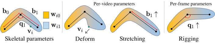
Figure 3: Skeletal shape parametric model. Our parametric model consists of joint angles $\mathbf{q}$, bone length $\mathbf{b}$, skinning weight $\mathbf{w}$, and vertex positions $\mathbf{v}$. Joint angles $\mathbf{q}$ change per-frame and the others are universal. Utilizing this model, animal shapes are tuned by vertex deformation as well as the stretching of bones. The target articulation would be fit by predicting per-frame joint angles.

3.1 Articulation model

Skeletal parameters. We exploit a stretchable bone-based skeletal model for our deformable shape parameterization ,as shown in Fig. 3. This articulated model consists of three components: 1) a triangular mesh consisting of a set of vertices and shapes in the canonical pose, describing the object’s shape; 2) a set of bones connected by a kinematic tree. Each one has a bone length parameter and associated rigging weight over each vertex; 3) a joint angle describing the relative transformation between each adjacent bone. To summarize, a deformed shape $\mathbf{s}_{t}$ at time $t$ can be represented as:

$$\mathbf{s}_{t}=\left\{\left\{\mathbf{v}_{i}\in{\mathbb{R}}^{3}\right\}_{N},\left\{\mathbf{f}_{j}\in\mathbb{I}^{3}\right\}_{T},\left\{\mathbf{w}_{i}\in\Delta^{K}\right\}_{N},\left\{b_{k}\in{\mathbb{R}}^{1}\right\}_{K},\left\{\mathbf{q}_{k}^{t}\in\mathbb{SO}(3)\right\}_{K}\right\}$$ (1)

where $\mathbf{v}_{i}$ is the vertex position, $\mathbf{f}_{j}$ represents a triangle face parameterized as a tuple of three vertex indices, $\mathbf{w}_{i}$ is the rigging weight constrained in a K-dimensional simplex: $\Delta^{K}=\left\{(w_{0},\dots,w_{K})\in\mathbb{R}^{K}~{}|~{}\sum_{k=0}^{K}w_{k}=1\textrm{ and }w_{k}\geq 0\right\}$; $b_{k}$ is the scalar bone length for each bone and $\mathbf{q}_{k}^{t}$ is the joint angle for each bone at a time $t$, represented as a unit quaternion in the $\mathbb{SO}(3)$ space. Note that all the variables except joint angles are shared across time.

Our skeletal model is grounded by the nature of many articulated objects. Unlike the commonly used control-point based articulation [41, 75, 74], our model reflects the constraints imposed by bones and joints, leading to more natural articulated deformation. Compared to category-specific parametric models [34, 85], it is more flexible and generalizable.

Forward kinematics. We use the forward kinematic model [26] to compute the transformation of each bone along the kinematic tree. Specifically, the rigid transformation of a bone is uniquely defined by the joint angles and bone length scales of the bone itself and its ancestors along the kinematic tree. Given a bone $k$, the rigid transform between its own frame and the root can be computed by recursively applying the relative rigid transformation along the chain:

$$\mathbf{T}_{k}^{t}(\mathbf{q}^{t}_{\textrm{\tiny{\tiny ans(k)}}},\mathbf{b}_{\textrm{\tiny{\tiny ans(k)}}})=\mathbf{T}_{\textrm{\tiny{\tiny pa}}(k)}^{t}\mathbf{T}^{t}_{k,\textrm{\tiny{pa}}(k)}(\mathbf{q}_{k}^{t},b_{k})=\prod_{k\prime\in\textrm{\tiny{ans}}(k)}\mathbf{T}^{t}_{k^{\prime},\textrm{\tiny{pa}}(k^{\prime})}(\mathbf{q}_{k^{\prime}}^{t},b_{k^{\prime}})$$ (2)

where $\mathbf{T}_{k}^{t}$,$\mathbf{T}_{\textrm{\tiny{\tiny pa}}(k)}^{t}$ is the transformation of bone $k$ and its parent node at frame $t$. $\mathbf{q}_{\textrm{\tiny{\tiny ans(k)}}},\mathbf{b}_{\textrm{\tiny{\tiny ans(k)}}}$ are the joint angles and bone lengths from all the ancestors of target bone $k$. $\mathbf{T}^{t}_{k,\textrm{\tiny{pa}}(k)}(\mathbf{q}_{k}^{t},b_{k})$ is the relative rigid transform between the bone and its parent frame, consists of a joint center translation along z axis decided by the bone length $b_{k}\mathbf{e}_{z}=[0,0,b_{k}]$ and a rotation around the joint center $\mathbf{R}(\mathbf{q}^{t}_{k})$.

Linear Blend Skinning (LBS). Given the rigid transformation of each bone, we adopt LBS to compute the transform of each point. Specifically, the deformation of each point $\mathbf{v}$ is decided by a linear composing the rigid transforms of bones through its skinning weight: $\mathbf{v}_{i}^{t}=\sum_{k=0}^{K}w_{i,k}\mathbf{T}_{k}^{t}\mathbf{v}_{i}$ where $w_{i,k}$ is the rigging weight. $\mathbf{T}_{k}^{t}$ is the transformation of bone $k$ at frame $t$ as defined in Eq. 2. For simplicity, we omit its dependent variables.

Stretchable bones. The aforementioned nonrigid deformation assumes independent shape and bone lengths. Naturally, the shape should deform accordingly as bone length changes. To model such a relationship, we exploit a stretchable bone deformation model [15]. For each bone, we compute an additional scaling transform along the bone vector direction based on its bone length change and apply this scaling transform to any points associated with this bone. Fig. 3 provides an illustration of stretching. For mathematical details on stretching, we refer readers to our supplementary document.

Stretchable bones bring a two-fold advantage: 1) it allows us to model shape variations within the same topological structures; 2) it makes the topological structure adjustable by “shrinking” the bones, e.g., a quadrupedal animal can be evolved into a seal-like skeletal model through optimization.

Reparameterization. Optimizing each vertex position offers flexibility yet might lead to undesirable mesh due to the lack of regularization. We use a neural displacement field to re-parameterize the vertex deformation to incorporate regularization, such as smooth and structured vertex deformation. We use a coordinate-based multi-layer perceptron (MLP) to define this displacement field $\mathcal{V}$. In addition, we incorporate a global scale scalar $\mathbf{u}$ in our framework to handle the shape misalignment between our initialization and the target. The position of each vertex is defined as:

$$\mathbf{v}_{i}^{\prime}=u\mathbf{v}_{i}+\mathcal{V}_{\theta}(u\mathbf{v}_{i})$$ (3)

where $u\mathbf{v}_{i}$ is the scaled position at the canonical pose, $\mathcal{V}_{\theta}(u\mathbf{p}_{i})$ represents the vertex offset parameterized by $\theta$, and $\mathbf{v}_{i}^{\prime}$ is the updated position for vertex $i$. During inference, instead of directly optimizing $\mathbf{v}_{i}$, we will only optimize the parameters of the displacement network. This displacement field reparameterization allow us to smoothly deform canonical shape during inference. In practice we find this implicit regularization compares favorably over explicit smoothness terms such as as-rigid-as-possible and laplacian smoothness.

3.2 Video-to-shape retrieval

Directly optimizing all skeletal parameters defined in Eq. 1 is challenging due to the variability and highly structured skeletal parameterization. Many deformable objects share similar topology structures, albeit with significant shape differences. To address it, we propose initializing skeletal shapes in a data-driven manner by choosing the best matching template from an asset bank.

Videos and skeletal shapes are in two different modalities; hence establishing a similarity measure is hard. Inspired by the recent success of language-vision pretraining models for 3D [66, 39], we utilize realistic rendering and pretraining image embedding models [47] to bridge this gap. Specifically, we first pre-render video footage for each character in the asset bank through a physically based renderer [7]. The environment lighting, background, articulated poses, and camera pose for each video are randomized to gain diversity and robustness. We then extract the image embedding features for each video using CLIP [47], which is a language-vision embedding model that is pretrained on a large-scale image-caption dataset. It captures the underlying semantic similarity between images well despite the large appearance and viewpoint difference. This is particularly suitable for retrieving shapes with similar kinematic structures, as the kinematics of animals is often related to semantics.

During inference, we extract embedding features from a given input video and measure the L2 distance between the input video and the rendered video of each object in the embedding space. We then select the highest-scoring articulated shape as the retrieved character. Please refer to the supplementary material for implementation details.

3.3 Neural inverse graphics via energy minimization

We expect our final output skeletal shape to 1) be consistent with the input video observation; 2) reflect prior knowledge about articulated shapes ,such as symmetry and smoothness. Inspired by this, we formulate ours as an energy minimization problem.

Energy formulation. We exploit visual cues from each frame including segmentation mask $\{\mathbf{M}_{t}\}$ and optical flow $\{\mathbf{F}_{t}\}$ through off-the-shelf neural networks [63, 74]. We also incorporate two types of prior knowledge, including the motion smoothness for joint angles $\mathbf{q}_{k}^{t}$ of bones across frames, as well as the symmetry constraint for the per-vertex offset $\mathbf{v}_{i}$ at the reference frame. In particular, let $\mathcal{I}=(\{\mathbf{I}_{t}\},\{{\mathbf{M}}_{t}\},\{{\mathbf{F}}_{t}\})$ be the input video frames and corresponding visual cues, and $\{\mathbf{s}_{t}\}$ be the predicted shapes of all frames, we formulate the energy for minimization as:

$$\min\limits_{\{\mathbf{s}_{t}\}_{1...T}}\lambda_{1}E_{\textrm{\tiny{\tiny cue}}}(\{\mathbf{s}_{t}\},\mathcal{I})+\lambda_{2}E_{\textrm{\tiny{smooth}}}({\{\mathbf{s}_{t}\}})+\lambda_{3}E_{\textrm{\tiny{symm}}}(\{\mathbf{s}_{t}\})$$ (4)

where $E_{\textrm{\tiny{\tiny cue}}}$ measures the consistency between the articulated shape and the visual cues; $E_{\textrm{\tiny{smooth}}}$ promotes smooth transitions overtime; $E_{\textrm{\tiny{symm}}}$ encodes the fact that many articulated objects are symmetric. The three energy terms complement each other, helping our model capture motions of the object according to visual observations, as well as constraining the deformed object to be natural and temporally consistent. We describe details of each term below.

Visual cue consistency. The visual cue consistency energy measures the agreement between the rendered maps of the articulated shape and 2D evidence (flow and silhouettes) from videos. We use a differentiable renderer [33] to generate projected object silhouettes $\{\mathbf{M}_{t}\}$. Additionally, we project vertices of predicted shapes at two consecutive frames to the camera view and compute the projected 2D displacement to render optical flow, following the prior work [74]. We leverage PointRend [22] for object segmentation and volumetric correspondence net [73] for flow prediction. The energy measures the difference between the rendered and inferred cues in $\ell_{2}$ distance:

$$E_{\textrm{\tiny{cue}}}=\sum_{t}\left\{\|\mathbf{M}_{t}-\pi_{\textrm{\tiny{seg}}}(\mathbf{s}_{t})\|^{2}+\beta\|\mathbf{F}_{t}-\pi_{\textrm{\tiny{flow}}}(\mathbf{s}_{t})\|^{2}\right\}$$ (5)

where $\beta$ is the trade-off weight; $\pi_{\textrm{\tiny{flow}}}(\mathbf{s}_{t})$ is the rendered the 2D flow map for each pixel given the deformed shape $\mathbf{s}_{t}$; $\pi_{\textrm{\tiny{seg}}}(\mathbf{s}_{t})$ is the rendered object mask. Similar to previous inverse rendering work [75], the object-camera transform is encoded as the root node transform.

Motion smoothness. This energy term encodes that motions of animals should be smooth and continuous across frames. We impose a constraint to ensure that there is little difference in joint angles of one bone from two consecutive frames should be slight. We implement this by computing the multiplication of the joint quaternion at the current frame and the inverse of the joint quaternion at the next frame, which should be close to an identity quaternion $\mathbf{q}=(0,0,0,1)$:

$$E_{\textrm{\tiny{smooth}}}=\sum_{t}\sum_{k}\|(\mathbf{q}_{k}^{t})^{-1}\circ\mathbf{q}_{k}^{t+1}-\mathbf{q}\|^{2}$$ (6)

where $\circ$ is the quaternion composition operator.

Symmetry offset. This term encourages the resulting shape in canonical space to be symmetric at the reference frame. It is inspired by the fact that most animals in the real world are symmetric if putting them into a certain canonical pose (e.g., ‘T-pose‘ for bipedal animals). Following previous works [74], we enforce this property at the canonical shape (where the joint angles are all zero). Specifically, we calculate the chamfer distance for measuring the similarity between the set of vertices $\{\mathbf{v}_{i}\}$ under the canonical shape and its reflection:

$$E_{\textrm{\tiny{symm}}}=\mathcal{L}_{\textrm{\tiny{cham}}}((\{\mathbf{v}_{i}\}),\mathbf{H}(\{\mathbf{v}_{i}\}))$$ (7)

where $\mathbf{H}$ is the Householder reflection matrix.

3.4 Inference

We reason the skeletal shape by minimizing the energy defined in Eq. 4. Our optimization variables include the vertex position $\mathbf{v}_{i}$ at the canonical pose, the rigging weight $\mathbf{w}_{i}$, bone length $\mathbf{b}_{k}$ as well as the joint angles $\mathbf{q}_{k}^{t}$. All the variables except joint angles are shared across time, and joint angles are optimized per frame.

Initialization. We initialize the vertex position, bone length, and the rigging weight $\mathbf{v}_{i},\mathbf{b}_{k},\mathbf{w}_{i}$ of canonical shape using the retrieved template character. The skeleton tree structure of this character is also taken as the basis of our skeletal parameterization. We initialize all the joint rotations as a unit quaternion.

Optimization. The energy function is fully differentiable and can be optimized end-to-end. We use Adam optimizer [21] to learn all the optimization variables. We adopt a scheduling strategy to avoid getting stuck at a local minimum. Specifically, we first optimize the mesh scaling factor based on silhouette correspondences. We then jointly update the bone length scale, joint angles, and the neural offset field by minimizing the energy function defined in Eq. 4.

Table 1: Quantitative results on PlanetZoo.

Method	mIoU $\uparrow$	mCham $\downarrow$	Skinning $\downarrow$	Joint $\downarrow$	Re-animation $\downarrow$
ViSER [75]	0.190	0.133	6.398	0.416	0.028
LASR [74]	0.306	0.094	2.576	0.158	0.033
CASA (ours)	0.512	0.053	3.288	0.089	0.010

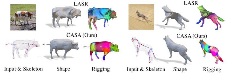
Figure 4: Reconstructed articulated shape. Top-left: input; top: LASR; bottom: ours.

4 PlanetZoo dataset

Benchmarking 4D animal reconstruction requires a large amount of nonrigid action sequences with ground truth articulated 3D shapes. Towards this goal, we construct a synthetic dataset PlanetZoo consisting of hundreds of animated animals with textures and skeletons from different categories. Appendix Fig. 12 depicts a snapshot of the assets and rendering images from our dataset, demonstrating the diversity and quality.

Data generation. We extracted animal meshes from the zoo simulator Planetzoo [35]. Cobra-tools [12] are used to extract those meshes along with their skeleton. With the extracted mesh and skeleton, we further render RGB maps, segmentation masks and optical flow for each frame using Blender.

Assets. To set a diverse environment, we set the background with random HDRI pictures for environmental lighting, and set floor textures with random materials from ambientCG. To reduce the gap between synthetic and real, we set the location of the light source along with its strength to simulate different environments in real-world situations.

Camera. To generate realistic action sequences, we randomly change camera locations between every 12 frames, resulting in a constant view-point change following the animal. The camera is allowed to rotate at a certain angle, ranging from $15^{\circ}$ to $22.5^{\circ}$.

Articulation. In order to obtain animated animal sequences, for every 12 frames, 8 bones are selected from the skeleton tree with a transformation attached. The angle value of rotation for each bone is sampled from a uniform distribution. By doing this, we are able to cover the whole action space, providing diverse action sequences.

Rendering. We generate silhouettes, optical flow, depth map, camera parameters, and RGB images using Vision Blender [7]. The physically based renderer is capable of showing fine details such as fur, making the rendering results more realistic. For each animal in the dataset, 180 frames are rendered.

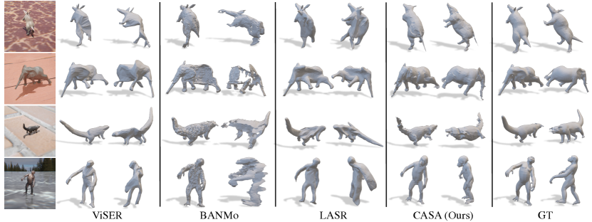
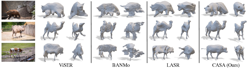
Figure 5: Qualitative comparison of our method on PlanetZoo.

Figure 6: Qualitative comparison of our method on real-world videos from DAVIS.

5 Experiments

In this section, we first introduce our experimental setting (§ 5.1). We then compare CASA  against a comprehensive set of articulated baselines in various reconstruction and articulation metrics on both simulation (§ 5.2) and real-world datasets (§ 5.3). Finally, we demonstrate our inferred shape can be used for downstream reanimation tasks (§ 5.4).

5.1 Experimental setup

Benchmarks. We validate our proposed method on two datasets. Our proposed photorealistic rendering dataset PlanetZoo as well as a real-world animal video dataset DAVIS[46], containing multiple real animal videos with mask annotations. For PlanetZoo, we choose 24 out of 249 total animals for testing and use the rest for validation and training. The testing dataset includes diverse articulated animals from unseen categories, including multiple quadrupeds, bipeds, birds categories, as well as unseen articulated topology such as pinnipeds.
Metrics. We measure the reconstruction quality by Intersection over Union (IOU) and Chamfer distance, as well as skinning distance, joint distance and re-animation quality on PlanetZoo.

1) mean Intersection Over Union(mIOU) measures the volumetric similarity between two shapes. We voxelized the reference and the predicted shape into occupancy grids and calculate the IOU ratio.

2) mean Chamfer Distance(mCham) computes the bidirectional vertex-to-vertex distances between the reference and the predicted shape.

3) Joint is the symmetric Chamfer Distance between joints. We evaluate CD-J2J following [72]. Given a predicted shape, we compute the Euclidean distance between each joint and its nearest joint in the reference shape, then divide it by the total joint number.

4) Skinning distance measures the similarity between the skinning weights. We first extract vertices associated with each joint using skinning weight. For each pair of joints from GT and prediction, we calculate the Chamfer distance between their associated vertices. Finally, we exploit the Jonker-Volgenant algorithm to find the minimum distance matching between prediction and reference.

5) Re-animation measures how well we can re-pose an articulated shape to a target shape. Specifically, we minimize the Chamfer Distance between the reference shape and the predicted shape by optimizing the joint angles of each bone for skeletal shape, or the rigid transform for control point-based shape. We consider this a holistic metric that jointly reflects the quality of shapes, skinning, and skeleton.

Baselines. We compare with state-of-the-art approaches for monocular-video articulated shape reconstruction ,including LASR [74], ViSER [75], and BANMo [76]. Similar to our method, they utilize 2D supervision of videos for training including segmentation masks and optical flows. We download the open-source version of them from GitHub. For the input data, we use our ground truth silhouette either in PlanetZoo dataset or DAVIS[46] dataset. We follow the optimization scripts in their code and get the baseline results.

3D reconstruction from a monocular video inevitably brings scale ambiguities. To alleviate the issue of scale differences, for every predicted shape among all the competing baselines, we conduct a line search to find the optimal scale that maximizes the IOU between the reference and the predicted shape.

5.2 Results on PlanetZoo

We present quantitative results on PlanetZoo in Tab. 1. CASA achieves higher performance on metrics mIOU and mCham, demonstrating a shape with higher fidelity. Our approach also outperforms other competing methods in reanimation, demonstrating the superior performance of holistic articulated shape reasoning and the potential for downstream reanimation tasks. CASA compares less favorably to LASR in the skinning quality. We conjecture this is due to additional degrees of freedom benefits brought by joint control point articulation.

Fig. 4 and Fig. 6 depict a few qualitative examples of all competing algorithms on PlanetZoo. We show the reconstructed mesh from both the camera view and the opposite view. The figure shows that CASA can recover accurate shape across various view angles under partial observation. In contrast, baselines fail to reconstruct reliable 3D mesh when the objects are partially observed. In addition, CASA also produces meshes with higher fidelity and local details in the visible region.

5.3 Real-world reconstruction

We demonstrate qualitative results of the competing algorithms on the real-world animal video dataset DAVIS [46] in Fig 6 and Fig. 4. This figure shows that both our method and baselines can get good reconstruction results from the camera perspective. But both two baselines fail to reconstruct those unseen parts. In contrast, CASA can reliably reason the shape and articulation in the unseen regions, thanks to its symmetry constraints, skeletal parameterization, and 3D template retrieval.

Figure 7: Reanimation results.

5.4 Reanimation

We now show how the reconstructed articulated 3D shape can be retargeted to new poses. Given an inferred skeletal shape and the target GT shape at a different articulated pose, we apply an inverse kinematic to compute the articulated pose to reanimate the inferred shape. Specifically, we optimize the articulated transforms such that the reanimated mesh is as close to the target in Chamfer distance. Joint quaternions are optimized for skeletal mesh, and the articulation transforms are optimized for the control-point-based method [74]. Fig. 7 shows a comparison between the retargeted meshes of our methods and LASR on PlanetZoo, with a GT target mesh as a reference. We observe that our retargeted meshes look realistic and accurate and preserve geometric details. Despite having more degrees of freedom in reanimation, LASR fails to produce realistic retarget results. Tab. 1 reports a quantitative comparison in chamfer distance between the retargeted and the reference mesh, demonstrating our approach outperforms competing methods by a large margin.

Table 2: Ablation study on energy terms

Method	mIOU $\uparrow$	mCham $\downarrow$	Skinning $\downarrow$	Joint $\downarrow$
CASA	0.512	0.053	3.288	0.089
w/o $E_{\textrm{\tiny{mask}}}$	0.011	*	*	*
w/o $E_{\textrm{\tiny{flow}}}$	0.427	0.350	3.290	0.636
w/o $E_{\textrm{\tiny{symm}}}$	0.387	*	4.008	*
w/o $E_{\textrm{\tiny{smooth}}}$	0.449	0.041	3.228	0.330

Table 3: Ablation study on optimization settings.

Method	mIOU $\uparrow$	mCham $\downarrow$	Skinning $\downarrow$	Joint $\downarrow$
CASA	0.512	0.053	3.288	0.089
w/o offset	0.144	0.343	3.174	0.783
w/o disp. field	0.235	0.055	3.218	0.262
w/o skeleton	0.372	0.060	3.245	N/A
w/o scaling	0.299	0.072	3.329	0.356

Table 4: Ablation study on our retrieval strategy.

Method	mIOU $\uparrow$	mCham $\downarrow$	Skinning $\downarrow$	Joint $\downarrow$
CASA	0.512	0.053	3.288	0.089
Retrieval-only (CLIP)	0.217	0.448	4.108	0.303
Retrieval (ImageNet)	0.111	0.972	4.295	0.813

Table 5: Ablation study on initialization settings.

Method	mIOU $\uparrow$	mCham $\downarrow$	Skinning $\downarrow$	Joint $\downarrow$
CASA (retrieval init)	0.512	0.053	3.288	0.089
k-means rigging init	0.305	0.452	3.336	0.659
Fixing skinning weight	0.433	0.052	3.235	0.318

5.5 Ablation study

We provide an ablation study to demonstrate the efficacy of each design choice in our framework.

Energy terms. In Tab. 4, we ablate different terms of our energy function. Specifically, we consider the mask consistency, flow consistency, symmetry and smoothness regularization separately. We find that the mask part is crucial for the performance, while the optical flow part also improves the framework results. Removing the symmetry offset term results in performance degradation since this term plays a vital role in regularizing the neural offset, which can alleviate issues brought by the ambiguity of single-view monocular video. The smooth term leads to better qualitative results.

Optimization. We compare different optimization settings in Tab. 3. The results show that: 1) using neural offset field is superior to per-vertex offset or not deforming shape (CASA vs. w/o offset vs. w/o disp. field); stretchable skeleton helps (CASA vs. w/o skeleton); removing shape scaling step leads to performance degradation (CASA vs. w/o scaling).

Retrieval strategies. In Tab. 5, we test different retrieval strategies. Our result demonstrates that CLIP is the preferred backbone for retrieval, most likely due to training with significantly richer semantic information than ImageNet pretrained models.

Initialization. We test different initialization strategies for skinning weights in Tab. 5. We replace the rigging from the retrieved animal by using k-means for initializing weights. The comparison in the table shows that high-quality rigging weight initialization is essential for good shape predictions. The results of sphere initialization also confirm the necessity of the proposed retrieval phase.

Stretchable bone. Fig. 8 shows qualitative results with/without stretchable bone parameterization. Compared to merely deforming each vertex, stretchable bone deformation ensures global consistency and smoothness. As noted in the figure, without stretchable bones, we see discontinuity at the nose of the animal and a mismatch between the lower and upper mouth.

5.6 Limitations

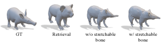
Figure 8: Stretchable bone

While demonstrating superior performance in animal reconstruction, our method has a few remaining drawbacks. Firstly, the source asset bank restricts the diversity of the retrieved articulation topology. Bone length optimization partially alleviates such limitations through “shrinking” bones. Still, it cannot add new bones to the kinematic tree, e.g., we cannot create a spider from a quadrupedal template. Secondly, our method so far does not impose the constraint that bones are inside the mesh. We plan to tackle such challenges in the future.

6 Conclusion

In this paper, we propose CASA, a novel category-agnostic animation reconstruction algorithm. Our method can take a monocular RGB video and predict a 4D skeletal mesh, including the surface, skeleton structure, skinning weight, and the joint angle at each frame. Our experimental results show that the proposed method achieves state-of-the-art performances in two challenging datasets. Importantly, we demonstrate that we could retarget our reconstructed 3D skeletal character and generate new animated sequences.

Acknowledgements. The authors thank Vlas Zyrianov and Albert Zhai for their feedback on the writing. The project is partially funded by the Illinois Smart Transportation Initiative STII-21-07. We also thank Nvidia for the Academic Hardware Grant.

Checklist

1. For all authors…

   1. Do the main claims made in the abstract and introduction accurately reflect the paper’s contributions and scope? [Yes]

   2. Did you describe the limitations of your work? [Yes]

   3. Did you discuss any potential negative societal impacts of your work? [Yes]

   4. Have you read the ethics review guidelines and ensured that your paper conforms to them? [Yes]

2. If you are including theoretical results…

   1. Did you state the full set of assumptions of all theoretical results? [N/A]

   2. Did you include complete proofs of all theoretical results? [N/A]

3. If you ran experiments…

   1. Did you include the code, data, and instructions needed to reproduce the main experimental results (either in the supplemental material or as a URL)? [No] we will release the code and data upon acceptance

   2. Did you specify all the training details (e.g., data splits, hyperparameters, how they were chosen)? [Yes]

   3. Did you report error bars (e.g., with respect to the random seed after running experiments multiple times)? [No]

   4. Did you include the total amount of compute and the type of resources used (e.g., type of GPUs, internal cluster, or cloud provider)? [Yes] We use eight GTX 2080 Ti and RTX A6000 GPUs.

4. If you are using existing assets (e.g., code, data, models) or curating/releasing new assets…

   1. If your work uses existing assets, did you cite the creators? [Yes]

   2. Did you mention the license of the assets? [No]

   3. Did you include any new assets either in the supplemental material or as a URL? [No] upon acceptance

   4. Did you discuss whether and how consent was obtained from people whose data you’re using/curating? [Yes] BADJA is open-sourced; PlanetZoo has commercial license, following prior practices in our community [51, 6, 14], we will ask users to purchase the game before accessing the dataset.

   5. Did you discuss whether the data you are using/curating contains personally identifiable information or offensive content? [Yes] Both datasets do not contain personal identifiable information.

5. If you used crowdsourcing or conducted research with human subjects…

   1. Did you include the full text of instructions given to participants and screenshots, if applicable? [N/A]

   2. Did you describe any potential participant risks, with links to Institutional Review Board (IRB) approvals, if applicable? [N/A]

   3. Did you include the estimated hourly wage paid to participants and the total amount spent on participant compensation? [N/A]

Appendix A Additional Results

We provide additional qualitative results on animals from PlanetZoo in Fig. 9. As shown in the figure, CASA well recovers the shape and topology of target animals from input videos. The sample of ostrich in this figure illustrates the limitations of CASA: 1) partial observation from monocular video leads to ambiguity on animal poses. The predicted shape fits well with the target from the camera view. However, from an alternative view, we can find that the wings of the prediction are of a wrong pose; 2) we do not impose a constraint on bones that they should be inside the mesh, resulting in joints in the head becoming outside the shape.

In order to demonstrate that CASA is able to adjust the topology of the initial shape, we provide the evolution of predictions for a seal in Fig. 10. Although the retrieved animal is a quadrupedal animal (otter), CASA gradually warps the predicted shapes to the target seal, whose topology is significantly different from quadrupeds.

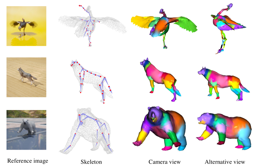
Figure 9: Additional qualitative results on PlanetZoo.

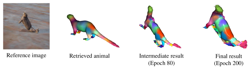
Figure 10: Given a retrieved animal with wrong articulation topology, CASA can recover a reasonable skeletal shape through our thanks to our stretchable bone formulation.

Appendix B Implementation Details

We minimize the energy function using Adam optimizer [21] with $\beta_{1}=0.9$ and $\beta_{2}=0.999$. We optimize the framework for $200$ epochs in total. A scheduling strategy is adopted. We optimize a scaling factor for the first 60 epochs by minimizing the mask term. This factor is initialized by aligning the bounding boxes between the rendering mask of the initial shape and the ground-truth mask. For the rest 140 epochs, we jointly optimize the bone length scale, joint angles, and the neural offset field. The learning rate is set to $5e-2$ for the first stage and $4e-3$ for all parameters in the second stage, except for the mesh scale and neural offset, which are set to $1e-3$. The trade-off weights for the mask term, flow term, smoothing term, and symmetry term are empirically set to $1e4$, $1e6$, $1e6$, and $1e4$, respectively. The neural offset field is parameterized by a four-layer MLP.

Appendix C Retrieval Result

Fig. 11 shows some retrieval results. Input animals are of various colors, skinning textures, and poses, together with different backgrounds and lighting conditions in their corresponding videos. Still, our method can retrieve animals from the database with a similar topology to the input, as CLIP [66] captures high-level semantic information and avoids distractions brought by different appearances and background environments. The sample of the seal at the bottom right is a failure case, as the two animals have different typologies. However, as shown in Fig. 10, CASA is able to bridge the gap between retrieved and target animals.

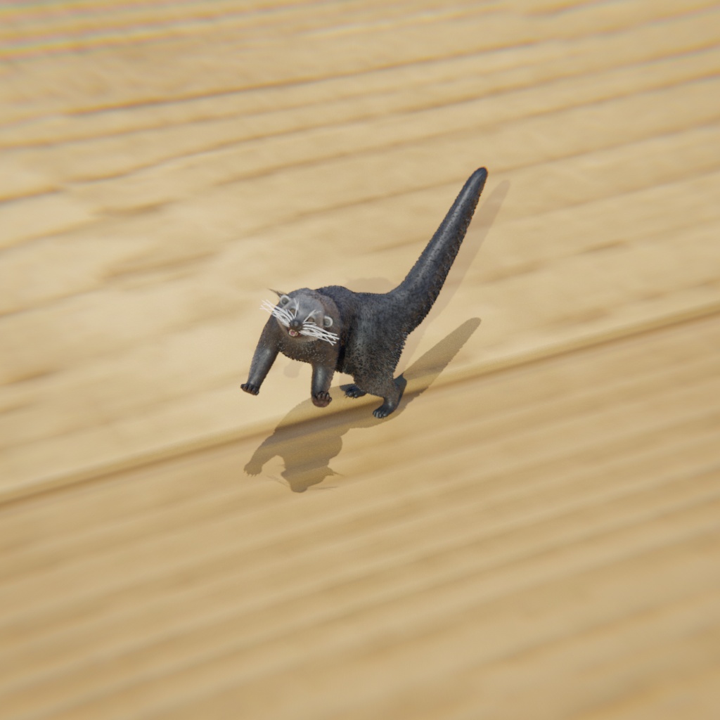
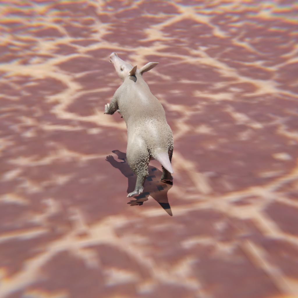
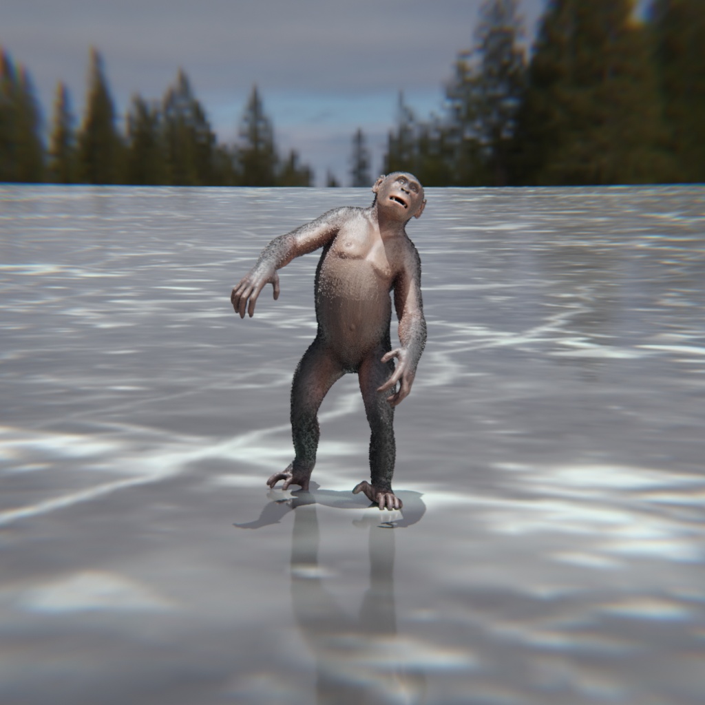
Input animal

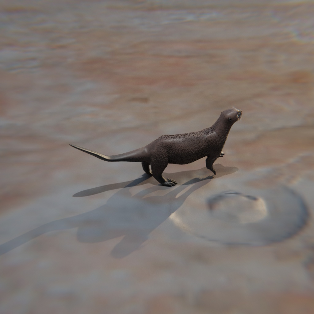
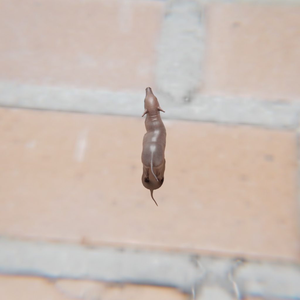
Retrieved animal

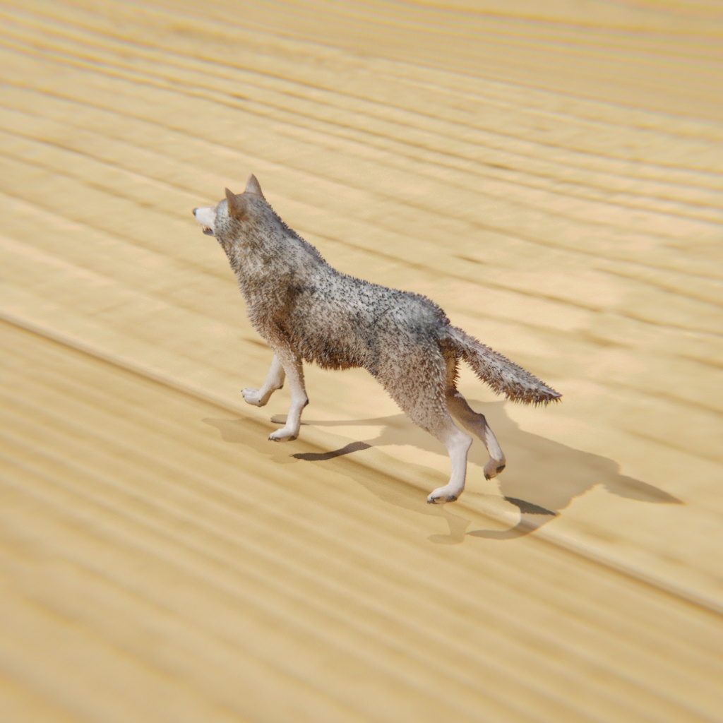
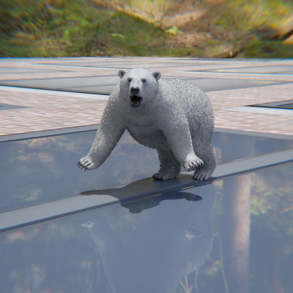
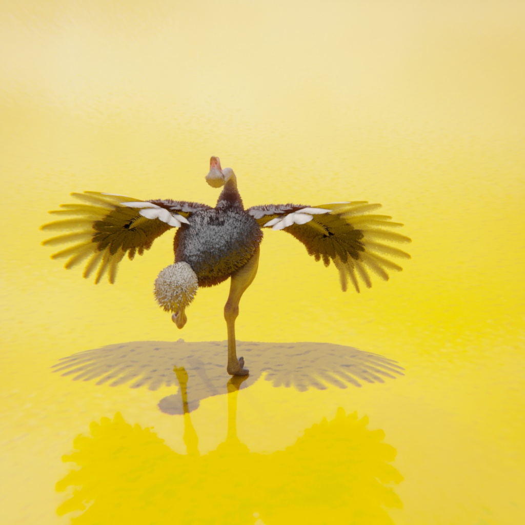
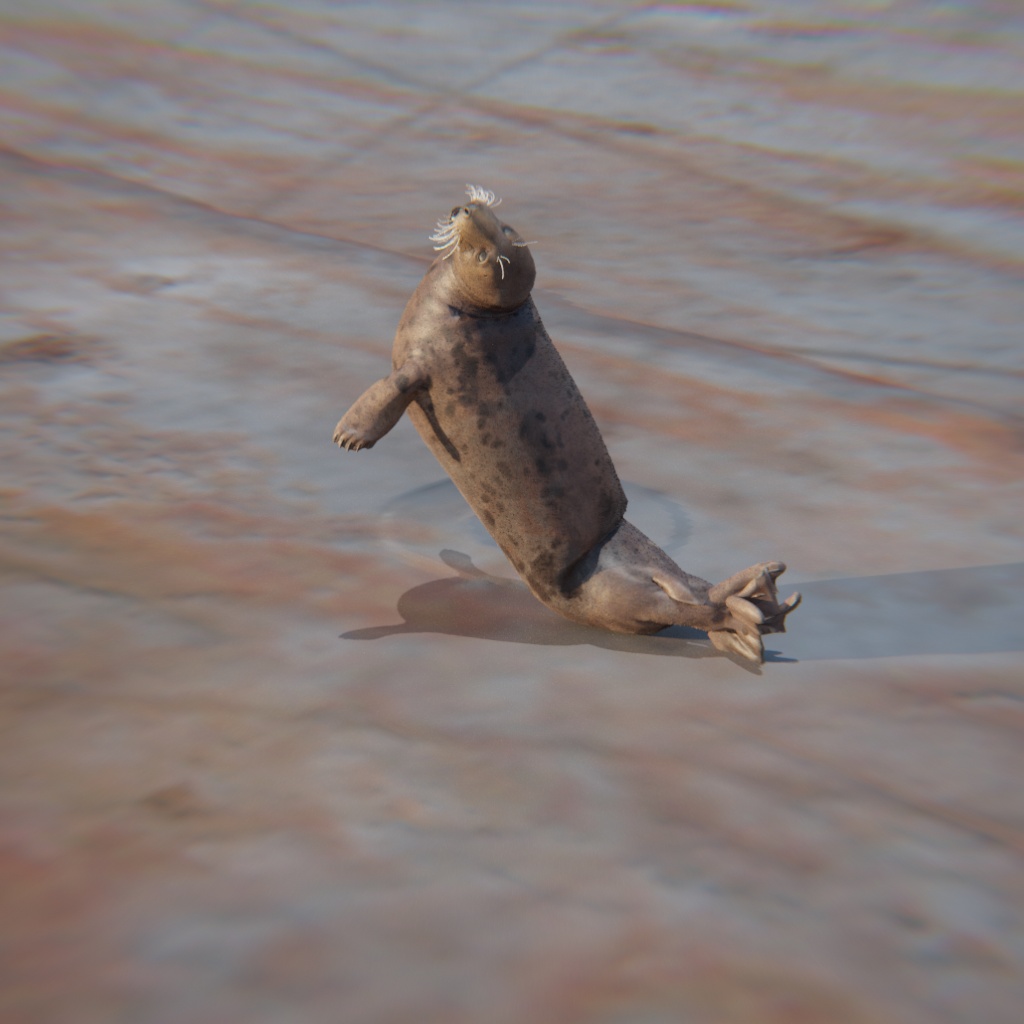
Input animal

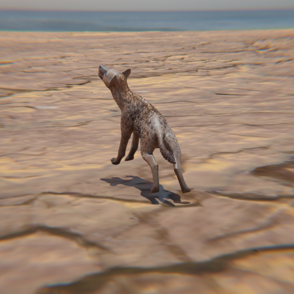
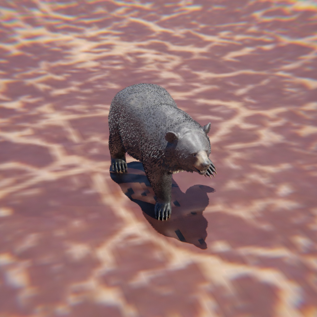
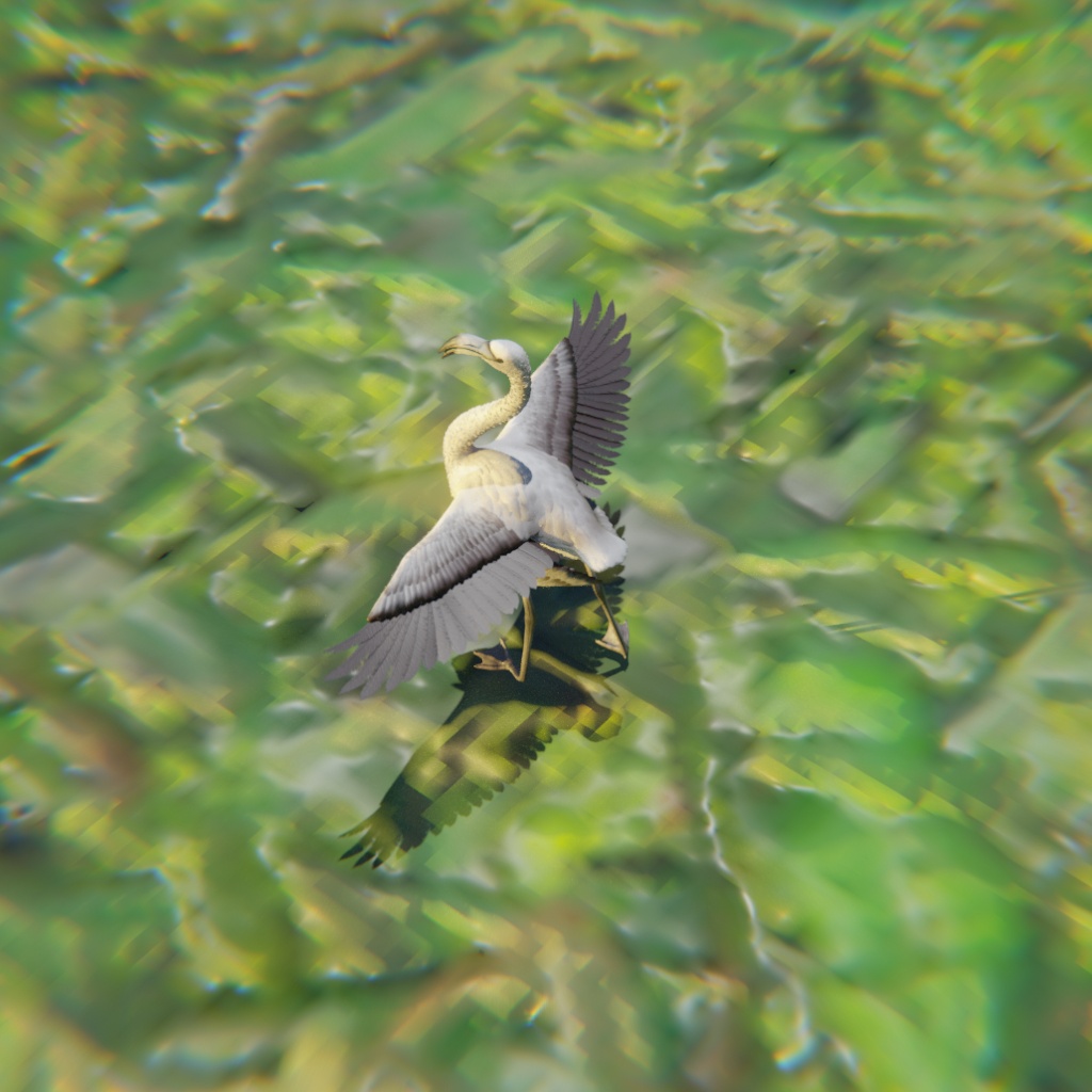
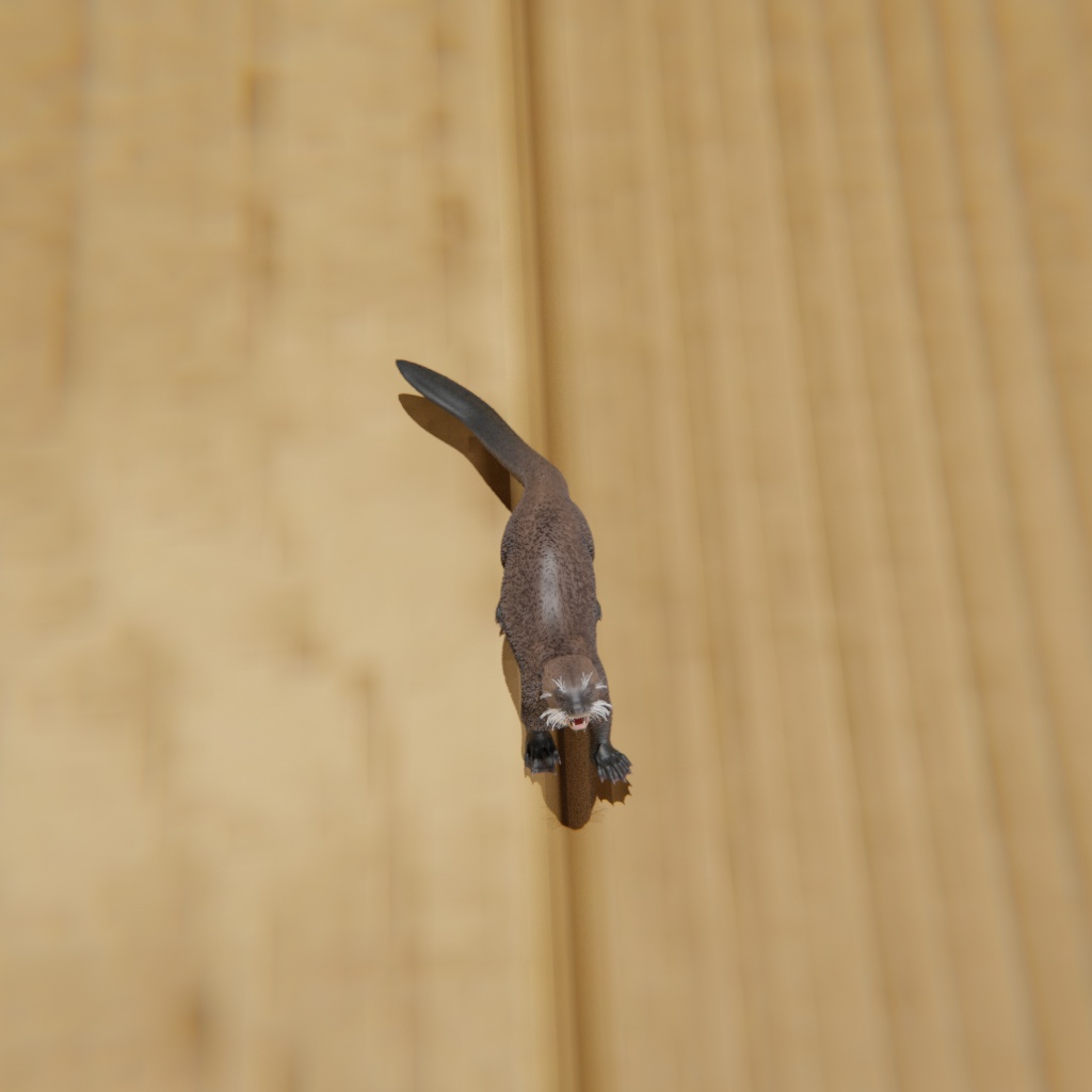
Retrieved animal

Figure 11: Retrieval results.

Appendix D Stretchable Bone Formulation

To incorporate stretchable bone parameterization into our linear blend skinning model, we have to re-formulate the skinning equation. The original formulation for linear blend skinning is defined as:

$$\mathbf{v}_{i}^{t}=\sum_{k=0}^{K}w_{i,k}\mathbf{T}_{k}^{t}\mathbf{v}_{i}$$ (8)

where $\mathbf{v}_{i}^{t}$ and $\mathbf{v}_{i}$ are the position of vertex $i$ at frame $t$ and the rest pose, respectively. $w_{i,k}$ is the rigging weight. $\mathbf{T}_{k}^{t}$ is the transformation of bone $k$ at frame $t$.

Since the bone transformation $\mathbf{T}_{k}^{t}$ is rigid, we can replace it by a translation and a rotation. In particular, given the head positions of each bone before and after deformation (which can be calculated by performing transformations according to forward kinematics), we can define the skinning model as:

$$\mathbf{v}_{i}^{t}=\sum_{k=0}^{K}w_{i,k}(\mathbf{c}_{i}^{t}+\mathbf{R}_{k}^{t}(-\mathbf{c}_{i}+\mathbf{v}_{i}))$$ (9)

where $\mathbf{c}_{k}$ and $\mathbf{c}_{k}^{t}$ are the head positions of bone $k$ before and after deformation. $\mathbf{R}_{k}^{t}$ is the rotation matrix decomposed from the rigid transformation $\mathbf{T}_{k}^{t}$.

Simply adding a scaling term into the skinning model can result in shape explosion, especially for vertices located near tails of bones, as illustrated in [15]. Following the solution proposed in [15], we define endpoint weight functions $e_{k}(\mathbf{p})$ for all bones, to control shape deformation in scaling. With the functions, the new skinning model is defined as:

$$\mathbf{v}_{i}^{t}=\sum_{k=0}^{K}\mathbf{w}_{i,k}(\mathbf{c}_{k}^{t}+R_{k}^{t}(e_{k}(\mathbf{p}_{i})\mathbf{s}_{k}+(\mathbf{p}_{i}-\mathbf{c}_{k}))$$ (10)

where $\mathbf{s}_{k}=(\mathbf{b}_{k}-1)(\mathbf{d}_{i}-\mathbf{c}_{i})$ is the full stretching vector at the tail of bone $\mathbf{d}_{i}$, $\mathbf{b}_{k}$ is the bone scaling factor. Each vertex $\mathbf{p}_{i}$ should have a unique stretching vector corresponding to this bone, which is decided by the endpoint weight function $e_{k}(\mathbf{p}_{i})$.

Typically the value of endpoint weight functions increases from 0 to 1 along the rest vector $(\mathbf{d}_{k}-\mathbf{c}_{k})$ of each bone. We define these functions by projecting each vertex $\mathbf{v}_{i}$ onto the nearest point of each bone, calculating the fraction of where it falls between the head and tail of the bone as the weight:

$$e_{k}(\mathbf{v}_{i})=\frac{\|\textrm{proj}_{k}(\mathbf{v}_{i})-\mathbf{c}_{k}\|}{\|\mathbf{d}_{k}-\mathbf{c}_{k}\|}$$ (11)

where $\mathbf{c}_{k}$ and $\mathbf{d}_{k}$ are the head and tail positions of bone $k$, $\textrm{proj}_{k}(\mathbf{v}_{i})$ is the projection of $\mathbf{v}_{i}$ onto the bone.

Appendix E Template-based Baseline

We compare CASA with an additional template-based baseline in Tab. 6. In order to ensure a fair comparison, we only incorporate quadruped animals in the PlanetZoo testset in experiments since ACFM is a category-specific method. The results show that CASA outperforms ACFM without pre-training on a large-scale database.

Table 6: Quantitative results on quadruped animals in PlanetZoo testset.

Method	mIOU $\uparrow$	mCham $\downarrow$
A-CFM [23]	0.234	0.246
CASA	0.499	0.050

Appendix F Optimization Framework Comparison

We compare CASA-retrieval + LASR with the entire CASA pipeline. For LASR, rather than using the whole coarse-to-fine optimization steps, we utilized only the final step. The quantitative comparison can be found in table 7.

Table 7: Optimization Comparison on PlanetZoo testset.

Method	mIOU $\uparrow$	mCham $\downarrow$	Skinning $\downarrow$	Joint$\downarrow$
Retrieval+LASR	0.191	0.158	2.975	0.407
CASA	0.512	0.053	3.288	0.089

Appendix G Efficiency

We conduct a comparison on the efficiency between CASA and the other two state-of-the-art methods, LASR [74] and ViSER [75]. We test their average running time for animals in the testing set of PlanetZoo, using one RTX 2080Ti. The results are shown in Tab. 8. Our method is approximately 3$\times$ faster than LASR and 5$\times$ faster than ViSER, demonstrating that our method is highly efficient. This is natural as CASA do not need to train any complex neural networks.

Table 8: Running time (min)

Method	ViSER	LASR	CASA
Time	234.2	144.6	46.7

Appendix H Detailed Implementation of Retrieval

We denote the input monocular video containing an animal to be reconstructed as $\{I_{t}\}_{t=1,...,T_{1}}$. The 3D asset bank for retrieving includes $N$ categories of animals. For each animal $i$, the asset bank includes a 3D mesh $M^{i}$, a skeleton $S^{i}$ and a realistic rendering video $\{I_{t}\}_{t=1,...,T_{2}}$. In our retrieval stage, our goal is to search the animal with the best similarity to the input animal in the asset bank, and the output should be its 3D shape $\mathbf{s}_{j}$. In short, our retrieval stage learns a mapping function from 2D video to 3D mesh. Since the input and output of retrieval are in different modalities, the target mapping function is not easy to learn. We propose to measure the similarity of the input video $\{I_{t}\}$ and all rendering videos in the asset bank using CLIP, obtain the most similar rendering video $\{I^{r}_{t}\}$, and take the corresponding animal mesh $M^{r}$ as the retrieval result.

To be specific, given the input video and any animal shape in the asset bank, we utilize pre-trained CLIP to encode all frames of the input video and the photo-realistic rendering :

$$\{F^{\mathrm{input}}_{t}\}_{t=1,...,T_{1}}=\{g_{\mathrm{CLIP}}(\{I_{t}\}\}_{t=1,...,T_{1}}$$

$$\{F^{j}_{v}\}_{v=1,...,V}=\{g_{\mathrm{CLIP}}(\pi(\mathbf{s}_{j},\mathbf{q}_{v})\}_{v=1,...,V}$$

where $\{I_{t}\}\}_{t=1,...,T_{1}}$ is the input video, $\mathbf{s}_{j}$ is the $j$-th animal shape, $g_{\mathrm{CLIP}}$ is the image embedding network of the CLIP model and $\pi(\mathbf{s}_{j},\mathbf{q}_{v})$ is the photo-realistic rendering of the articulated shape $\mathbf{s}_{j}$ at a randomized skeletal poses $\mathbf{q}_{v}$. $T_{1}$ is the length of the input video. $V$ is the number of randomized skeletal pose. Note that we render only one frame for each pose.

With the corresponding encoding features $\{F^{\mathrm{input}}_{t}\}$ and $\{F^{j}_{v}\}$, we first calculate the similarity $D$ between the $t$-th input frame and the $v$-th skeletal pose for the $j$-th shape by:

$$S(I_{t},\pi(\mathbf{s}_{j},\mathbf{q}_{v}))=\|F^{\mathrm{input}}_{t}-F^{j}_{v}\|^{2}_{2}$$

With the similarity defined above, We are able to retrieve the animal category $r$ in the asset bank that is the most similar with the input animal, which is formulated as:

$$r=\arg\max_{j}\max_{t}\max_{v}S(I_{t},\pi(\mathbf{s}_{j},\mathbf{q}_{v}))$$

We then obtain the 3D animal shape $\mathbf{s}_{r}$ together with its corresponding skeleton and skinning weight from the asset bank, which is used for initializing the following optimization process.

Appendix I Initialization Strategy of CASA

We provide details of our initialization strategy for CASA.

In the skeletal optimization stage of CASA, optimizing parameters include a displacement field, the skinning weight, joint rotation angles for each bone, a root transformation, and bone length scales. During initialization, the displacement field is defined by a Multi-Layer Perception (MLP) with random network parameters. The skinning weight is set according to the retrieval results. Bone length scales are all set to 1. The joint angles are set to T-pose.

The root transformation is represented as a combination of rotation and translation. For the convergence of skeletal optimization, the root transformation should ensure the consistency of the mesh in the camera coordinate with the ground-truth. Instead of estimating such transformation in world coordinate, we propose to predict camera parameters for each video, and fix the root transformation as an identical one. In practice, for synthetic videos in which the camera parameters are available, we directly use them as initialization. For videos where camera parameters are not available, we adopt a naive strategy to predict the camera parameters.

Specifically, we first optimize the camera intrinsic and focus point offset from the origin by minimizing the mask loss between rendering and ground-truth. In each iteration, we randomly sample a point as the location of the camera from a sphere with its center at the origin and radius $R$ set according to the animal scale.

When meeting the convergence criteria, we fix the camera intrinsic and focus point offset. We then pick camera locations sampled before with the Top-10 lowest mask loss values. For each location, we randomly sample points in its nearby regions as new camera locations, calculate the corresponding mask loss values, and select the location with the lowest value as our final camera location.

Appendix J More information on PlanetZoo

We provide the names of all categories in PlanetZoo in Tab. LABEL:tab:all_names. We also show an overview figure of PlanetZoo in Fig. 12.

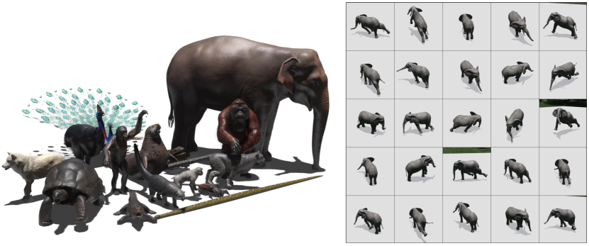
Figure 12: Overview of PlanetZoo. We collect a novel dataset PlanetZoo containing high-fidelity and animatable 3D animal models. On the right we show renderings for the elephant with different poses.

Table 9: Names of all categories in PlanetZoo.

aardvark female	aardvark juvenile	aardvark male
african buffalo female	african buffalo juvenile	african buffalo male
african elephant female	african elephant juvenile	african elephant male
african wild dog female	african wild dog juvenile	african wild dog male
aldabra giant tortoise female	aldabra giant tortoise juvenile	aldabra giant tortoise male
amazonian giant centipede	american bison female	american bison juvenile
american bison male	arctic wolf female	arctic wolf juvenile
arctic wolf male	babirusa female	babirusa juvenile
babirusa male	bactrian camel female	bactrian camel juvenile
bactrian camel male	bairds tapir female	bairds tapir juvenile
bairds tapir male	bengal tiger female	bengal tiger juvenile
bengal tiger male	binturong female	binturong juvenile
binturong male	black wildebeest female	black wildebeest juvenile
black wildebeest male	boa constrictor	bongo female
bongo male	bonobo female	bonobo juvenile
bonobo male	bornean orangutan female	bornean orangutan juvenile
bornean orangutan male	brazilian salmon pink tarantula	brazilian wandering spider
capuchin monkey female	capuchin monkey juvenile	capuchin monkey male
cassowary female	cassowary juvenile	cassowary male
cheetah female	cheetah juvenile	cheetah male
chinese pangolin female	chinese pangolin juvenile	chinese pangolin male
clouded leopard female	clouded leopard juvenile	clouded leopard male
common ostrich female	common ostrich juvenile	common ostrich male
common warthog female	common warthog juvenile	common warthog male
cuviers dwarf caiman female	cuviers dwarf caiman juvenile	cuviers dwarf caiman male
dall sheep female	dall sheep juvenile	dall sheep male
death adder	dhole female	dhole juvenile
dhole male	diamondback terrapin	dingo female
dingo juvenile	dingo male	eastern blue tongued lizard
eastern brown snake	formosan black bear female	formosan black bear juvenile
formosan black bear male	galapagos giant tortoise female	galapagos giant tortoise juvenile
galapagos giant tortoise male	gemsbok female	gemsbok juvenile
gemsbok male	gharial female	gharial juvenile
gharial male	giant anteater female	giant anteater juvenile
giant anteater male	giant burrowing cockroach	giant desert hairy scorpion
giant forest scorpion	giant leaf insect	giant otter female
giant otter juvenile	giant otter male	giant panda female
giant panda juvenile	giant panda male	gila monster
golden poison frog	goliath beetle	goliath birdeater
goliath frog	gray wolf female	gray wolf juvenile
gray wolf male	greater flamingo female	greater flamingo juvenile
greater flamingo male	green iguana	grey seal female
grey seal juvenile	grey seal male	grizzly bear female
grizzly bear juvenile	grizzly bear male	himalayan brown bear female
himalayan brown bear juvenile	himalayan brown bear male	hippopotamus female
hippopotamus juvenile	hippopotamus male	indian elephant female
indian elephant juvenile	indian elephant male	indian peafowl juvenile
indian peafowl male	indian rhinoceros female	indian rhinoceros juvenile
indian rhinoceros male	jaguar female	jaguar juvenile
jaguar male	japanese macaque female	japanese macaque juvenile
japanese macaque male	king penguin female	king penguin juvenile
king penguin male	koala female	koala juvenile
koala male	komodo dragon female	komodo dragon juvenile
komodo dragon male	lehmanns poison frog	lesser antillean iguana
llama female	llama juvenile	llama male
malayan tapir female	malayan tapir juvenile	malayan tapir male
mandrill female	mandrill juvenile	mandrill male
mexican redknee tarantula	nile monitor juvenile	nile monitor male
nyala female	nyala juvenile	nyala male
okapi female	okapi juvenile	okapi male
plains zebra female	plains zebra juvenile	plains zebra male
polar bear female	polar bear juvenile	polar bear male
proboscis monkey female	proboscis monkey juvenile	proboscis monkey male
pronghorn antelope female	pronghorn antelope juvenile	pronghorn antelope male
puff adder	pygmy hippo female	pygmy hippo juvenile
pygmy hippo male	red eyed tree frog	red kangaroo female
red kangaroo juvenile	red kangaroo male	red panda juvenile
red panda male	red ruffed lemur female	red ruffed lemur juvenile
red ruffed lemur male	reindeer female	reindeer juvenile
reindeer male	reticulated giraffe female	reticulated giraffe juvenile
reticulated giraffe male	ring tailed lemur juvenile	ring tailed lemur male
sable antelope female	sable antelope juvenile	sable antelope male
saltwater crocodile female	saltwater crocodile juvenile	saltwater crocodile male
siberian tiger female	siberian tiger juvenile	siberian tiger male
snow leopard female	snow leopard juvenile	snow leopard male
spotted hyena female	spotted hyena juvenile	spotted hyena male
springbok female	springbok juvenile	springbok male
sun bear female	sun bear juvenile	sun bear male
thomsons gazelle female	thomsons gazelle juvenile	thomsons gazelle male
titan beetle	west african lion female	west african lion juvenile
west african lion male	western chimpanzee female	western chimpanzee juvenile
western chimpanzee male	western diamondback rattlesnake	western lowland gorilla female
western lowland gorilla juvenile	western lowland gorilla male	yellow anaconda

Table 10: Full retrieval results.

Input animal	Retrieval animal
aardvark female	koala female
aardvark juvenile	arctic wolf juvenile
aardvark male	babirusa juvenile
african elephant female	indian elephant male
african elephant male	indian elephant juvenile
african elephant juvenile	indian elephant juvenile
binturong female	giant otter male
binturong juvenile	cuviers dwarf caiman female
binturong male	cuviers dwarf caiman female
grey seal female	babirusa juvenile
grey seal juvenile	koala juvenile
grey seal male	giant otter female
bonobo juvenile	bornean orangutan juvenile
bonobo male	western chimpanzee juvenile
bonobo female	western chimpanzee juvenile
polar bear female	formosan black bear male
polar bear juvenile	spotted hyena juvenile
polar bear male	grizzly bear male
gray wolf female	spotted hyena female
gray wolf juvenile	arctic wolf juvenile
gray wolf male	spotted hyena male
common ostrich female	american bison juvenile
common ostrich juvenile	babirusa juvenile
common ostrich male	greater flamingo juvenile

References

- [1] Dragomir Anguelov, Praveen Srinivasan, Daphne Koller, Sebastian Thrun, Jim Rodgers, and James Davis. Scape: shape completion and animation of people. In SIGGRAPH, 2005.
- [2] Benjamin Biggs, Oliver Boyne, James Charles, Andrew Fitzgibbon, and Roberto Cipolla. Who left the dogs out? 3d animal reconstruction with expectation maximization in the loop. In ECCV, 2020.
- [3] Volker Blanz and Thomas Vetter. A morphable model for the synthesis of 3d faces. In Computer graphics and interactive techniques, 1999.
- [4] Federica Bogo, Javier Romero, Gerard Pons-Moll, and Michael J Black. Dynamic FAUST: Registering human bodies in motion. In CVPR, 2017.
- [5] Christoph Bregler, Aaron Hertzmann, and Henning Biermann. Recovering non-rigid 3d shape from image streams. In CVPR, 2000.
- [6] Zhe Cao, Hang Gao, Karttikeya Mangalam, Qizhi Cai, Minh Vo, and Jitendra Malik. Long-term human motion prediction with scene context. In ECCV, 2020.
- [7] João Cartucho, Samyakh Tukra, Yunpeng Li, Daniel S. Elson, and Stamatia Giannarou. Visionblender: a tool to efficiently generate computer vision datasets for robotic surgery. Computer Methods in Biomechanics and Biomedical Engineering: Imaging & Visualization, 2020.
- [8] Angel X Chang, Thomas Funkhouser, Leonidas Guibas, Pat Hanrahan, Qixing Huang, Zimo Li, Silvio Savarese, Manolis Savva, Shuran Song, Hao Su, et al. Shapenet: An information-rich 3d model repository. arXiv:1512.03012, 2015.
- [9] Alexey Dosovitskiy, German Ros, Felipe Codevilla, Antonio Lopez, and Vladlen Koltun. Carla: An open urban driving simulator. In CoRL, 2017.
- [10] Shubham Goel, Angjoo Kanazawa, and Jitendra Malik. Shape and viewpoint without keypoints. In ECCV, 2020.
- [11] Kaiwen Guo, Peter Lincoln, Philip Davidson, Jay Busch, Xueming Yu, Matt Whalen, Geoff Harvey, Sergio Orts-Escolano, Rohit Pandey, Jason Dourgarian, et al. The relightables: Volumetric performance capture of humans with realistic relighting. ACM TOG, 2019.
- [12] HENDRIX-ZT2. cobra-tools. https://github.com/OpenNaja/cobra-tools, 2020.
- [13] Yuan-Ting Hu, Jiahong Wang, Raymond A Yeh, and Alexander G Schwing. SAIL-VOS 3D: A Synthetic Dataset and Baselines for Object Detection and 3D Mesh Reconstruction from Video Data. In CVPR, 2021.
- [14] Yuan-Ting Hu, Jiahong Wang, Raymond A Yeh, and Alexander G Schwing. Sail-vos 3d: A synthetic dataset and baselines for object detection and 3d mesh reconstruction from video data. In CVPR, 2021.
- [15] Alec Jacobson and Olga Sorkine. Stretchable and twistable bones for skeletal shape deformation. In SIGGRAPH Asia, 2011.
- [16] Justin Johnson, Bharath Hariharan, Laurens Van Der Maaten, Li Fei-Fei, C Lawrence Zitnick, and Ross Girshick. Clevr: A diagnostic dataset for compositional language and elementary visual reasoning. In CVPR, 2017.
- [17] Hanbyul Joo, Tomas Simon, Xulong Li, Hao Liu, Lei Tan, Lin Gui, Sean Banerjee, Timothy Scott Godisart, Bart Nabbe, Iain Matthews, Takeo Kanade, Shohei Nobuhara, and Yaser Sheikh. Panoptic studio: A massively multiview system for social interaction capture. PAMI, 2017.
- [18] Angjoo Kanazawa, Michael J Black, David W Jacobs, and Jitendra Malik. End-to-end recovery of human shape and pose. In CVPR, 2018.
- [19] Angjoo Kanazawa, Shubham Tulsiani, Alexei A Efros, and Jitendra Malik. Learning category-specific mesh reconstruction from image collections. In ECCV, 2018.
- [20] Ladislav Kavan, Steven Collins, Jiří Žára, and Carol O’Sullivan. Geometric skinning with approximate dual quaternion blending. ACM TOG, 2008.
- [21] Diederik P Kingma and Jimmy Ba. Adam: A method for stochastic optimization. In ICLR, 2015.
- [22] Alexander Kirillov, Yuxin Wu, Kaiming He, and Ross Girshick. Pointrend: Image segmentation as rendering. In CVPR, 2020.
- [23] Filippos Kokkinos and Iasonas Kokkinos. Learning monocular 3d reconstruction of articulated categories from motion. In CVPR, 2021.
- [24] Chen Kong and Simon Lucey. Deep non-rigid structure from motion. In ICCV, 2019.
- [25] Nilesh Kulkarni, Abhinav Gupta, David F Fouhey, and Shubham Tulsiani. Articulation-aware canonical surface mapping. In CVPR, 2020.
- [26] Steven M LaValle. Planning algorithms. 2006.
- [27] Jiahui Lei and Kostas Daniilidis. Cadex: Learning canonical deformation coordinate space for dynamic surface representation via neural homeomorphism. In CVPR, 2022.
- [28] John P Lewis, Matt Cordner, and Nickson Fong. Pose space deformation: a unified approach to shape interpolation and skeleton-driven deformation. In SIGGRAPH, 2000.
- [29] Tianye Li, Timo Bolkart, Michael J Black, Hao Li, and Javier Romero. Learning a model of facial shape and expression from 4d scans. ACM TOG, 2017.
- [30] Xueting Li, Sifei Liu, Shalini De Mello, Kihwan Kim, Xiaolong Wang, Ming-Hsuan Yang, and Jan Kautz. Online adaptation for consistent mesh reconstruction in the wild. In NeurIPS, 2020.
- [31] Yang Li, Hikari Takehara, Takafumi, Taketomi, Bo Zheng, and Matthias Nießner. 4dcomplete: Non-rigid motion estimation beyond the observable surface. In ICCV, 2021.
- [32] Shaowei Liu, Hanwen Jiang, Jiarui Xu, Sifei Liu, and Xiaolong Wang. Semi-supervised 3d hand-object poses estimation with interactions in time. In CVPR, 2021.
- [33] Shichen Liu, Tianye Li, Weikai Chen, and Hao Li. Soft rasterizer: A differentiable renderer for image-based 3d reasoning. In ICCV, 2019.
- [34] Matthew Loper, Naureen Mahmood, Javier Romero, Gerard Pons-Moll, and Michael J Black. Smpl: A skinned multi-person linear model. ACM TOG, 2015.
- [35] Ingo Lütkebohle. PlanetZoo Simulator. https://www.planetzoogame.com/, 2021.
- [36] Wei-Chiu Ma, Anqi Joyce Yang, Shenlong Wang, Raquel Urtasun, and Antonio Torralba. Virtual correspondence: Humans as a cue for extreme-view geometry. In CVPR, 2022.
- [37] Nadia Magnenat-Thalmann, Richard Laperrire, and Daniel Thalmann. Joint-dependent local deformations for hand animation and object grasping. In Graphics interface, 1988.
- [38] Bruce Merry, Patrick Marais, and James Gain. Animation space: A truly linear framework for character animation. ACM TOG, 2006.
- [39] Oscar Michel, Roi Bar-On, Richard Liu, Sagie Benaim, and Rana Hanocka. Text2mesh: Text-driven neural stylization for meshes. In CVPR, 2022.
- [40] Marko Mihajlovic, Yan Zhang, Michael J Black, and Siyu Tang. LEAP: Learning articulated occupancy of people. In CVPR, 2021.
- [41] Richard A. Newcombe, Dieter Fox, and Steven M. Seitz. Dynamicfusion: Reconstruction and tracking of non-rigid scenes in real-time. In CVPR, 2015.
- [42] Michael Niemeyer, Lars Mescheder, Michael Oechsle, and Andreas Geiger. Occupancy flow: 4d reconstruction by learning particle dynamics. In ICCV, 2019.
- [43] Atsuhiro Noguchi, Umar Iqbal, Jonathan Tremblay, Tatsuya Harada, and Orazio Gallo. Watch it move: Unsupervised discovery of 3D joints for re-posing of articulated objects. In CVPR, 2022.
- [44] Pablo Palafox, Aljaž Božič, Justus Thies, Matthias Nießner, and Angela Dai. Npms: Neural parametric models for 3d deformable shapes. In ICCV, 2021.
- [45] Keunhong Park, Utkarsh Sinha, Jonathan T Barron, Sofien Bouaziz, Dan B Goldman, Steven M Seitz, and Ricardo Martin-Brualla. Nerfies: Deformable neural radiance fields. In ICCV, 2021.
- [46] F. Perazzi, J. Pont-Tuset, B. McWilliams, L. Van Gool, M. Gross, and A. Sorkine-Hornung. A benchmark dataset and evaluation methodology for video object segmentation. In CVPR, 2016.
- [47] Alec Radford, Jong Wook Kim, Chris Hallacy, Aditya Ramesh, Gabriel Goh, Sandhini Agarwal, Girish Sastry, Amanda Askell, Pamela Mishkin, Jack Clark, et al. Learning transferable visual models from natural language supervision. In ICML, 2021.
- [48] Aditya Ramesh, Prafulla Dhariwal, Alex Nichol, Casey Chu, and Mark Chen. Hierarchical text-conditional image generation with clip latents. arXiv:2204.06125, 2022.
- [49] Yongming Rao, Wenliang Zhao, Guangyi Chen, Yansong Tang, Zheng Zhu, Guan Huang, Jie Zhou, and Jiwen Lu. Denseclip: Language-guided dense prediction with context-aware prompting. In CVPR, 2022.
- [50] Zhongzheng Ren, Xiaoming Zhao, and Alex Schwing. Class-agnostic reconstruction of dynamic objects from videos. In NeurIPS, 2021.
- [51] Stephan R Richter, Zeeshan Hayder, and Vladlen Koltun. Playing for benchmarks. In ICCV, 2017.
- [52] Mike Roberts, Jason Ramapuram, Anurag Ranjan, Atulit Kumar, Miguel Angel Bautista, Nathan Paczan, Russ Webb, and Joshua M Susskind. Hypersim: A photorealistic synthetic dataset for holistic indoor scene understanding. In ICCV, 2021.
- [53] Javier Romero, Dimitrios Tzionas, and Michael J Black. Embodied hands: Modeling and capturing hands and bodies together. SIGGRAPH ASIA, 2017.
- [54] Nadine Rüegg, Silvia Zuffi, Konrad Schindler, and Michael J Black. Barc: Learning to regress 3d dog shape from images by exploiting breed information. In CVPR, 2022.
- [55] Shunsuke Saito, Zeng Huang, Ryota Natsume, Shigeo Morishima, Angjoo Kanazawa, and Hao Li. Pifu: Pixel-aligned implicit function for high-resolution clothed human digitization. In ICCV, 2019.
- [56] Shunsuke Saito, Tomas Simon, Jason Saragih, and Hanbyul Joo. Pifuhd: Multi-level pixel-aligned implicit function for high-resolution 3d human digitization. In CVPR, 2020.
- [57] Shunsuke Saito, Jinlong Yang, Qianli Ma, and Michael J Black. Scanimate: Weakly supervised learning of skinned clothed avatar networks. In CVPR, 2021.
- [58] Manolis Savva, Abhishek Kadian, Oleksandr Maksymets, Yili Zhao, Erik Wijmans, Bhavana Jain, Julian Straub, Jia Liu, Vladlen Koltun, Jitendra Malik, et al. Habitat: A platform for embodied ai research. In ICCV, 2019.
- [59] Bokui Shen, Fei Xia, Chengshu Li, Roberto Martín-Martín, Linxi Fan, Guanzhi Wang, Claudia Pérez-D’Arpino, Shyamal Buch, Sanjana Srivastava, Lyne Tchapmi, et al. igibson 1.0: A simulation environment for interactive tasks in large realistic scenes. In IROS, 2020.
- [60] Vikramjit Sidhu, Edgar Tretschk, Vladislav Golyanik, Antonio Agudo, and Christian Theobalt. Neural dense non-rigid structure from motion with latent space constraints. In ECCV, 2020.
- [61] Julian Straub, Thomas Whelan, Lingni Ma, Yufan Chen, Erik Wijmans, Simon Green, Jakob J. Engel, Raul Mur-Artal, Carl Ren, Shobhit Verma, Anton Clarkson, Mingfei Yan, Brian Budge, Yajie Yan, Xiaqing Pan, June Yon, Yuyang Zou, Kimberly Leon, Nigel Carter, Jesus Briales, Tyler Gillingham, Elias Mueggler, Luis Pesqueira, Manolis Savva, Dhruv Batra, Hauke M. Strasdat, Renzo De Nardi, Michael Goesele, Steven Lovegrove, and Richard Newcombe. The Replica dataset: A digital replica of indoor spaces. arXiv:1906.05797, 2019.
- [62] Chen Sun, Austin Myers, Carl Vondrick, Kevin Murphy, and Cordelia Schmid. Videobert: A joint model for video and language representation learning. In ICCV, 2019.
- [63] Zachary Teed and Jia Deng. Raft: Recurrent all-pairs field transforms for optical flow. In ECCV, 2020.
- [64] Shubham Tulsiani, Nilesh Kulkarni, and Abhinav Gupta. Implicit mesh reconstruction from unannotated image collections. arXiv:2007.08504, 2020.
- [65] Yael Vinker, Ehsan Pajouheshgar, Jessica Y Bo, Roman Christian Bachmann, Amit Haim Bermano, Daniel Cohen-Or, Amir Zamir, and Ariel Shamir. Clipasso: Semantically-aware object sketching. SIGGRAPH, 2022.
- [66] Can Wang, Menglei Chai, Mingming He, Dongdong Chen, and Jing Liao. Clip-nerf: Text-and-image driven manipulation of neural radiance fields. In CVPR, 2022.
- [67] Wenshan Wang, Delong Zhu, Xiangwei Wang, Yaoyu Hu, Yuheng Qiu, Chen Wang, Yafei Hu, Ashish Kapoor, and Sebastian Scherer. Tartanair: A dataset to push the limits of visual slam. In IROS, 2020.
- [68] Xiaohuan Corina Wang and Cary Phillips. Multi-weight enveloping: least-squares approximation techniques for skin animation. In SIGGRAPH, 2002.
- [69] Chung-Yi Weng, Brian Curless, Pratul P. Srinivasan, Jonathan T. Barron, and Ira Kemelmacher-Shlizerman. HumanNeRF: Free-viewpoint rendering of moving people from monocular video. In CVPR, 2022.
- [70] Shangzhe Wu, Tomas Jakab, Christian Rupprecht, and Andrea Vedaldi. Dove: Learning deformable 3d objects by watching videos. arXiv:2107.10844, 2021.
- [71] Hu Xu, Gargi Ghosh, Po-Yao Huang, Dmytro Okhonko, Armen Aghajanyan, Florian Metze, Luke Zettlemoyer, and Christoph Feichtenhofer. Videoclip: Contrastive pre-training for zero-shot video-text understanding. In EMNLP, 2021.
- [72] Zhan Xu, Yang Zhou, Evangelos Kalogerakis, Chris Landreth, and Karan Singh. Rignet: Neural rigging for articulated characters. ACM TOG, 2020.
- [73] Gengshan Yang and Deva Ramanan. Volumetric correspondence networks for optical flow. NeurIPS, 32, 2019.
- [74] Gengshan Yang, Deqing Sun, Varun Jampani, Daniel Vlasic, Forrester Cole, Huiwen Chang, Deva Ramanan, William T Freeman, and Ce Liu. LASR: Learning articulated shape reconstruction from a monocular video. In CVPR, 2021.
- [75] Gengshan Yang, Deqing Sun, Varun Jampani, Daniel Vlasic, Forrester Cole, Ce Liu, and Deva Ramanan. Viser: Video-specific surface embeddings for articulated 3d shape reconstruction. In NeurIPS, 2021.
- [76] Gengshan Yang, Minh Vo, Natalia Neverova, Deva Ramanan, Andrea Vedaldi, and Hanbyul Joo. Banmo: Building animatable 3d neural models from many casual videos. In CVPR, 2022.
- [77] Ze Yang, Siva Manivasagam, Ming Liang, Bin Yang, Wei-Chiu Ma, and Raquel Urtasun. Recovering and simulating pedestrians in the wild. In CoRL, 2020.
- [78] Ze Yang, Shenlong Wang, Sivabalan Manivasagam, Zeng Huang, Wei-Chiu Ma, Xinchen Yan, Ersin Yumer, and Raquel Urtasun. S3: Neural shape, skeleton, and skinning fields for 3d human modeling. In CVPR, 2021.
- [79] Renrui Zhang, Ziyu Guo, Wei Zhang, Kunchang Li, Xupeng Miao, Bin Cui, Yu Qiao, Peng Gao, and Hongsheng Li. Pointclip: Point cloud understanding by clip. In CVPR, 2022.
- [80] Xiaoming Zhao, Yuan-Ting Hu, Zhongzheng Ren, and Alexander G. Schwing. Occupancy Planes for Single-view RGB-D Human Reconstruction. In arXiv:2208.02817, 2022.
- [81] Jia Zheng, Junfei Zhang, Jing Li, Rui Tang, Shenghua Gao, and Zihan Zhou. Structured3d: A large photo-realistic dataset for structured 3d modeling. In ECCV, 2020.
- [82] Kaiyang Zhou, Jingkang Yang, Chen Change Loy, and Ziwei Liu. Learning to prompt for vision-language models. IJCV, 2022.
- [83] Silvia Zuffi, Angjoo Kanazawa, Tanya Berger-Wolf, and Michael J Black. Three-D Safari: Learning to Estimate Zebra Pose, Shape, and Texture from Images In the Wild. In ICCV, 2019.
- [84] Silvia Zuffi, Angjoo Kanazawa, and Michael J Black. Lions and tigers and bears: Capturing non-rigid, 3d, articulated shape from images. In CVPR, 2018.
- [85] Silvia Zuffi, Angjoo Kanazawa, David W Jacobs, and Michael J Black. 3d menagerie: Modeling the 3d shape and pose of animals. In CVPR, 2017.