Beyond Schwarzschild-de Sitter spacetimes: II.   An exact non-Schwarzschild metric in pure $R^{2}$ gravity and new anomalous properties of $R^{2}$ spacetime

Abstract

In a recent publication [Phys. Rev. D 106, 104004 (2022)], we advanced a program that Buchdahl originated but prematurely abandoned circa 1962 [Nuovo Cimento, Vol. 23, No 1, 141 (1962)]. Therein we obtained an exhaustive class of metrics that constitute the branch of non-trivial solutions to the pure $\mathcal{R}^{2}$ field equation in vacuo. The Buchdahl-inspired metrics in general possess non-constant scalar curvature, thereby defeating the generalized Lichnerowicz theorem advocated in (Nelson-2010, ; Lu-2015-a, ; Lu-2015-b, ; Luest-2015-backholes, ). We found that the said theorem makes an overly strong assumption on the asymptotic falloff in the spatial derivatives of the Ricci scalar, rendering it violable against the Buchdahl-inspired metrics. In this paper, we shall further extend our work mentioned above (Nguyen-2022-Buchdahl, ) by showing that, within the class of Buchdahl-inspired metrics, the asymptotically flat member takes on the following exact closed analytical expression

$$ds^{2}=\left|1-\frac{r_{\text{s}}}{r}\right|^{\frac{k}{r_{\text{s}}}}\left\{-\left(1-\frac{r_{\text{s}}}{r}\right)dt^{2}+\left(1-\frac{r_{\text{s}}}{r}\right)^{-1}\frac{\rho^{4}(r)}{r^{4}}\,dr^{2}+\rho^{2}(r)\,d\Omega^{2}\right\}$$

in which the areal coordinate $\rho$ is related to the radial coordinate $r$ per

$$\rho(r)=\frac{\zeta\,r_{\text{s}}\left|1-\frac{r_{\text{s}}}{r}\right|^{\frac{1}{2}\left(\zeta-1\right)}}{\left|1-\text{sgn}\Bigl{(}1-\frac{r_{\text{s}}}{r}\Bigr{)}\left|1-\frac{r_{\text{s}}}{r}\right|^{\zeta}\right|};\ \ \ \ \ \zeta:=\sqrt{1+3k^{2}/r_{\text{s}}^{2}}$$

The special Buchdahl-inspired metric, as we shall call it as such hereafter, is characterized by a “Schwarzschild” radius $r_{\text{s}}$ and the Buchdahl parameter $k$, the latter of which arises via the higher-derivative nature of $\mathcal{R}^{2}$ gravity. The case $k=0$ corresponds precisely to the classic Schwarzschild metric. Equipped with this exact expression, we shall investigate pure $\mathcal{R}^{2}$ spacetime structures. The asymptotically flat spacetime is split into an interior region and an exterior region, with the boundary situated at $\rho=r_{\text{s}}$. We find that, except for $k=0$ and $k=-r_{\text{s}}$, the Kretschmann invariant of this metric exhibits an additional singularity at the interior-exterior boundary. Accordingly, the surface area of the interior-exterior boundary is found to vanish for $k\in(-\infty,-r_{\text{s}})\cup(0,+\infty)$, diverge for $k\in(-r_{\text{s}},0)$, equal $4\pi r_{\text{s}}^{2}$ for $k=0$, and equal $16\pi r_{\text{s}}^{2}$ for $k=-r_{\text{s}}$. This behavior signals a naked singularity or a wormhole. We shall also analytically construct the Kruskal-Szekeres (KS) diagram for pure $\mathcal{R}^{2}$ spacetime. The Buchdahl parameter $k$ is found to modify the KS diagram in some fundamental way. A striking result is that the (modified) KS diagram develops a “gulf” that sandwiches between the four established quadrants. The “gulf” resides strictly on the interior-exterior boundary and does not correspond to any domain in the physical spacetime, specified by $\left(t,r,\theta,\phi\right)$. The nature of this novel “virtual” region in the KS diagram is an open question, related to which we make a conjecture on a possible path forward.

I Introduction:   Buchdahl’s $\boldsymbol{1962}$ program in pure $\mathcal{R}^{2}$ gravity

Pure $\mathcal{R}^{2}$ gravity is among the simplest candidates for modified gravity. Its action contains a single term, $\frac{1}{2\kappa}\int d^{4}x\sqrt{-g}\,\mathcal{R}^{2}$, with $\kappa$ being a dimensionless parameter, while the traditional Einstein-Hilbert term is suppressed. The theory was considered as early as the 1960’s by Buchdahl as a parsimonious prototype of higher-order gravity that possesses an additional symmetry – the scale invariance (Buchdahl-1962, ). There is a surge of interest in the pure $\mathcal{R}^{2}$ action of late (AlvarezGaume-2015, ; Alvarez-2018, ; Stelle-1977, ; Edery-2014, ) within a larger context of modified gravity (Capozziello-2011, ; Clifton-2011, ; deFelice-2010, ; Sotiriou-2008, ; Nojiri-2011, ; Nojiri-2017, ). Pure $\mathcal{R}^{2}$ gravity is the only theory that is both ghost-free and scale invariant (Stelle-1978, ; Luest-2015-fluxes, ).

In a seminal – yet obscure – 1962 Nuovo Cimento paper entitled “On the Gravitational Field Equations Arising from the Square of the Gaussian Curvature” (Buchdahl-1962, ), Buchdahl pioneered a program in search of static spherically symmetric vacua for pure $\mathcal{R}^{2}$ gravity. He established therein that the vacua in general possess non-constant scalar curvature, as a result of the higher-derivative structure of the theory. Surpassing several obstacles, his efforts culminated in a non-linear second-order ordinary differential equation (ODE) which required being solved. The finish line was within his striking distance: the $\mathcal{R}^{2}$ vacua Buchdahl sought after hinged on the analytical solution – yet to be found in his time – to the ODE he derived. Unfortunately, Buchdahl deemed his ODE intractable and prematurely suspended his pursuit for an analytical solution. Until our recent work (Nguyen-2022-Buchdahl, ), his ODE had remained untackled; and to this day, his Nuovo Cimento paper has largely gone unnoticed by the gravitation research community .

Recently, we have managed to bridge the remaining gap in the Buchdahl program by identifying a compact solution to his ODE (Nguyen-2022-Buchdahl, ). With this impasse finally overcome, we proceeded to accomplishing Buchdahl’s ultimate goal. The outcome is an exhaustive class of pure $\mathcal{R}^{2}$ vacua expressible in a compact form, which we called the Buchdahl-inspired solution, to be summarized below.

The Buchdahl-inspired solution

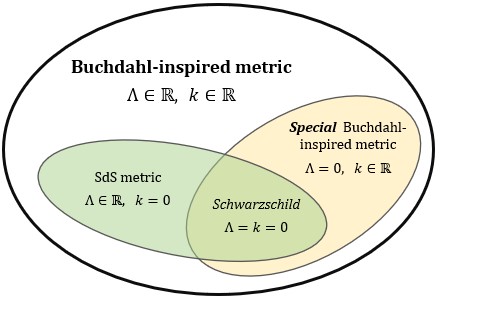
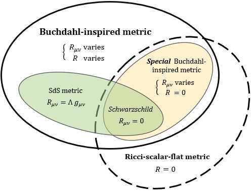
Figure 1: Upper panel: the Buchdahl-inspired metric family and its subsets. Lower panel: their relation with the Ricci-scalar-flat family. The special Buchdahl-inspired metric in the intersection is asymptotically flat, whereas the Buchdahl-inspired metric with $\Lambda\neq 0$ is asymptotically constant.

In (Nguyen-2022-Buchdahl, ) by reformulating Buchdahl’s original derivation which was quite cumbersome, we obtained the Buchdahl-inspired metric, cast in a parallel resemblance to the classic Schwarzschild-de Sitter (SdS) metric, per

$$ds^{2}=e^{k\int\frac{dr}{r\,q(r)}}\left\{p(r)\Bigl{[}-\frac{q(r)}{r}dt^{2}+\frac{r}{q(r)}dr^{2}\Bigr{]}+r^{2}d\Omega^{2}\right\}$$ (1)

The pair of functions $\{p(r),q(r)\}$ obey the “evolution” rules

$${\displaystyle\frac{dp}{dr}}\, ={\displaystyle\,\frac{3k^{2}}{4\,r}\frac{p}{q^{2}}}$$ (2)

$${\displaystyle{\displaystyle\frac{dq}{dr}}}\, =\,{\displaystyle\bigl{(}1-\Lambda\,r^{2}\bigr{)}\,p}$$ (3)

and the non-constant Ricci scalar equals to

$$\mathcal{R}(r)=4\Lambda\,e^{-k\int\frac{dr}{r\,q(r)}}$$ (4)

This metric is specified by two parameters, $\Lambda$ and $k$, resulted from the fourth-derivative nature of $\mathcal{R}^{2}$ gravity, a theory that requires two additional boundary conditions as compared with second-derivative theories, such as the Einstein-Hilbert action. If the spacetime structures associated with this metric are proven to be stable, then $k$ would stand for new higher-derivative hair which allows the Ricci scalar to vary on the manifold, per Eq. (4). At largest distances, the Ricci scalar converges to $4\Lambda$, characterizing an asymptotically constant spacetime.

To allay any lingering doubt, in (Nguyen-2022-Buchdahl, ) and (Shurtleff-2022, ) the current author and Shurtleff independently checked that the solution given in Eqs. (1)–(4) satisfies the pure $\mathcal{R}^{2}$ vacuo field equation

$$\mathcal{R}\Bigl{(}\mathcal{R}_{\mu\nu}-\frac{1}{4}g_{\mu\nu}\mathcal{R}\Bigr{)}+\Bigl{(}g_{\mu\nu}\,\square-\nabla_{\mu}\nabla_{\nu}\Bigr{)}\mathcal{R}=0$$ (5)

for all values of $\Lambda\in\mathbb{R}$ and $k\in\mathbb{R}$, thereby affirming its validity. We must stress that the solution presented above is able to defeat the generalized Lichnerowicz theorem advocated in (Nelson-2010, ; Lu-2015-a, ; Lu-2015-b, ; Luest-2015-backholes, ) by evading an overly strong condition on the asymptotic falloff in $D_{i}\mathcal{R}$ assumed in the theorem; see our companion papers in this “Beyond Schwarzschild–de Sitter spacetimes” series for a detailed exposition (Nguyen-2022-Buchdahl, ; Nguyen-2022-extension, ).

The most crucial element of the metric is the new (Buchdahl) parameter $k$ which makes the metric non-Schwarzschild. At $k=0$, the Buchdahl-inspired metric duly recovers the SdS metric. To see this, at $k=0$ the evolution rules (2)–(3) admit the solution $p(r)\equiv 1$ and $q(r)=r-\frac{\Lambda}{3}r^{3}-r_{\text{s}}$, with $r_{\text{s}}$ being a constant, upon which metric (1) is readily brought into the SdS form with a constant curvature $\mathcal{R}=4\Lambda$ everywhere. A non-zero value of $k$ would trigger a non-linear interplay between $p(r)$ and $q(r)$ per Eqs. (2)–(3) and enable a non-constant curvature to manifest, per Eq. (4).

The relations between the Buchdahl-inspired metric and the SdS metric as well as the null-Ricci-scalar spaces are depicted by the Venn diagrams in Fig. 1. By superseding the SdS metric, the Buchdahl-inspired spacetime is a bona fide enlargement of the SdS spacetime, suitably regarded as a framework “beyond Schwarzschild–de Sitter” (Nguyen-2022-Buchdahl, ).

The curious case of $\Lambda=0$

Also shown in Fig. 1 is the special Buchdahl-inspired metric which is the Buchdahl-inspired metric with $\Lambda$ set equal to zero. This special metric wholly occupies the intersection of the branch of (non-trivial) Buchdahl-inspired metrics and the branch of (trivial) null-Ricci-scalar spaces.

Surprisingly, despite being non-linear, the evolution rules (2) and (3) are fully soluble for $\Lambda=0$. In this paper we shall exploit this advantage to derive a closed analytical expression for the special Buchdahl-inspired metric.

Equipped with this exact analytical solution, we then are empowered to investigate the properties of $\mathcal{R}^{2}$ spacetime structures that live on an asymptotically flat background. These structures are described by the special Buchdahl-inspired metric.

—————–$\infty$—————–

Our paper is organized in four major sections. Sec. II is devoted to deriving the special Buchdahl-inspired metric. Sec. III produces a number of surprising properties in the Kretschmann invariant and the surface area of the interior-exterior boundary of $\mathcal{R}^{2}$ spacetime structures. Sec. IV analytically constructs a modified Kruskal-Szekeres (KS) diagram for the special Buchdahl-inspired metric and uncovers yet a novel feature of its KS diagram. Finally, Sec. V discusses the potential implications of our finding in various areas in modified gravity.

II Derivation of the special Buchdahl-inspired metric

This rather dense section derives the closed analytical solution in step-by-step details, with Lemma 13 being our ultimate result. We start with solving the evolution rules (2)–(3) for $\Lambda=0$ in Sec. II.1. We then, in Sec. II.2, expose the inadequacy of the standard Schwarzschild radial coordinate $r$ for this metric, resulting in the need for a new radial coordinate. Secs. II.3 and II.4 introduce two coordinate transformations in sequel that lead to the final solution, described in Sec. II.5.

II.1 Analytical solution to the evolution rules with $\Lambda=0$

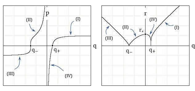
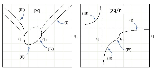
Figure 2: Plots of $p$, $r$, $pq$ and $pq/r$ as functions of $q$. Plots are for $r_{\text{s}}=1,\ k=r_{\text{s}}$. See Remark 4 for explanations.

Lemma 1.

For $\Lambda=0$, the set of equations (2)–(3) admits the following solution:

$$r =\left|q-q_{+}\right|^{\frac{q_{+}}{q_{+}-q_{-}}}\left|q-q_{-}\right|^{-\frac{q_{-}}{q_{+}-q_{-}}}$$ (6)

$$p =\frac{(q-q_{+})(q-q_{-})}{r\,q}$$ (7)

$$q_{\pm} :=\frac{1}{2}\left(-r_{\text{s}}\pm\sqrt{r_{\text{s}}^{2}+3k^{2}}\right)$$ (8)

with $r_{\text{s}}\in\mathbb{R}$ and $q_{\pm}$ representing the two real roots of the algebraic equation

$$q^{2}+r_{\text{s}}\,q-\frac{3k^{2}}{4}=0$$ (9)

Proof.

For $\Lambda=0$, the evolution rules (2)–(3) become

$$p_{r} =\frac{3k^{2}}{4r}\frac{p}{q^{2}}$$ (10)

$$q_{r} =p$$ (11)

which give

$$q_{rr}=\frac{3k^{2}}{4r}\frac{q_{r}}{q^{2}}$$ (12)

Upon a change of variable $r=e^{x}$:

$$q_{r} =\frac{dq}{dx}\frac{dx}{dr}=q_{x}\,e^{-x}$$ (13)

$$q_{rr} =\frac{d}{dx}\left(q_{x}e^{-x}\right)\frac{dx}{dr}=\left(q_{xx}-q_{x}\right)e^{-2x}$$ (14)

Equation (12) becomes

$$q_{xx}=\left(1+\frac{3k^{2}}{4q^{2}}\right)q_{x}$$ (15)

which can be recast as

$$\frac{d}{dx}\left(\frac{dq}{dx}\right)=\left(1+\frac{3k^{2}}{4q^{2}}\right)\frac{dq}{dx}$$ (16)

or, equivalently

$$\frac{d}{dq}\left(\frac{dq}{dx}\right)=1+\frac{3k^{2}}{4q^{2}}$$ (17)

Upon integrating, it yields a first-order ODE

$$\frac{dq}{dx}=q-\frac{3k^{2}}{4q}+r_{\text{s}}$$ (18)

with $r_{\text{s}}$ being an integration constant. Let $q_{\pm}:=\frac{1}{2}\left(-r_{\text{s}}\pm\sqrt{r_{\text{s}}^{2}+3k^{2}}\right)$ be the two real roots of the algebraic equation (9). A further integration of (18), with the integration constant for $x$ set equal zero without loss of generality, produces

$$x =\int\frac{q\,dq}{(q-q_{+})(q-q_{-})}$$ (19)

$$=\frac{q_{+}}{q_{+}-q_{-}}\ln|q-q_{+}|-\frac{q_{-}}{q_{+}-q_{-}}\ln|q-q_{-}|$$ (20)

Restoring $r=e^{x}$, we then obtain

$$r=\left|q-q_{+}\right|^{\frac{q_{+}}{q_{+}-q_{-}}}\left|q-q_{-}\right|^{-\frac{q_{-}}{q_{+}-q_{-}}}$$ (21)

Additionally, from (11) and (18), together with $x=\ln r$, we have

$$p =q_{r}=q_{x}\frac{dx}{dr}=q_{x}\,\frac{1}{r}$$ (22)

$$=\frac{1}{r}\left(q-\frac{3k^{2}}{4q}+r_{\text{s}}\right)$$ (23)

$$=\frac{1}{rq}(q-q_{+})(q-q_{-})$$ (24)

∎

Combining Lemma 1 with Eq. (1), we arrive at the following analytical result.

Corollary 2.

For $\Lambda=0$, the Buchdahl-inspired metric (1)–(3) is fully analytic, per

$$ds^{2} =e^{k\int\frac{dr}{r(q)q}}\biggl{\{}-\frac{p(q)q}{r(q)}dt^{2}+\frac{p(q)r(q)}{q}dr^{2}+r^{2}(q)d\Omega^{2}\biggr{\}}$$ (25)

$$r(q) =\left|q-q_{+}\right|^{\frac{q_{+}}{q_{+}-q_{-}}}\left|q-q_{-}\right|^{-\frac{q_{-}}{q_{+}-q_{-}}}$$ (26)

$$p(q) =\frac{(q-q_{+})(q-q_{-})}{r(q)\,q}$$ (27)

$$k =\left(-\frac{4}{3}q_{+}q_{-}\right)^{1/2}$$ (28)

Remark 3.

We shall call the Buchdahl-inspired metric with $\Lambda=0$ the special Buchdahl-inspired metric. We shall also choose a convention of $r_{\text{s}}>0$ in the rest of the paper. The case of $r_{\text{s}}=0$ is considered in Appendix A.

Remark 4.

Using Eqs. (26) and (27), we produce the plots of $p$, $r$, $pq$ and $pq/r$ against $q$, as shown in Fig. 2.The parameters are $k=r_{\text{s}}=1$, making $q_{+}=1/2$, $q_{-}=-3/2$, and $r_{*}:=\left|q_{+}\right|^{\frac{q_{+}}{q_{+}-q_{-}}}\left|q_{-}\right|^{-\frac{q_{-}}{q_{+}-q_{-}}}=(27)^{1/4}/2\approx 1.14$. In the upper left panel, the four quadrants of the ${p,q}$ diagram are labeled (I), (II), (III), (IV) counterclockwise, respectively. In the other three panels, the quadrant labels (as defined in the $\{p,q\}$ plot) are attached accordingly.

Remark 5.

From Eq. (27), it is straightforward to prove that the special Buchdahl-inspired metric supports a duality relation:

$$q\,p(q)=r(q_{+}+q_{-}-q)$$ (29)

Remark 6.

Note that $q_{-}<0<q_{+}$, by virtue of their definitions in Eq. (8). The zeros of $r$ and $p$ occur at $q=q_{+}$ and $q=q_{-}$. Furthermore,

$$p =\begin{cases}\ >0&\text{for }q\in(q_{-},0)\cup(q_{+},+\infty)\\ \ <0&\text{for }q\in(-\infty,q_{-})\cup(0,q_{+})\end{cases}$$ (30)

$$pq =\begin{cases}\ >0&\text{for }q\in(-\infty,q_{-})\cup(q_{+},+\infty)\\ \ <0&\text{for }q\in(q_{-},q_{+})\end{cases}$$ (31)

Remark 7.

From the duality relation (29) and the definition of $q_{\pm}$ in (8),

$$\frac{q\,p(q)}{r(q)}=\frac{r(q_{+}+q_{-}-q)}{r(q)}=\left|\frac{q-q_{+}}{q-q_{-}}\right|^{\frac{1}{\sqrt{1+3k^{2}/r_{\text{s}}^{2}}}}$$ (32)

making $\frac{q\,p}{r}$ vanish as $q\rightarrow q_{+}$ and diverge as $q\rightarrow q_{-}$. These behaviors account for the lower right panel in Fig. 2.

Remark 8.

As $q\rightarrow 0^{\pm}$, $r$ approaches $r_{*}:=\left|q_{+}\right|^{\frac{q_{+}}{q_{+}-q_{-}}}\left|q_{-}\right|^{-\frac{q_{-}}{q_{+}-q_{-}}}$, whereas $p\rightarrow\mp\infty$, respectively. One can also show that, for $q\in(q_{-},q_{+})$,

$$\frac{dr}{dq}=-q\left(q_{+}-q\right)^{\frac{q_{-}}{q_{+}-q_{-}}}\left(q-q_{-}\right)^{-\frac{q_{+}}{q_{+}-q_{-}}}$$ (33)

forcing $r(q)$ to peak at $q=0$ in the interval $(q_{-},q_{+})$. These behaviors explain the two upper panels in Fig. 2.

II.2 Problems with the Schwarzschild radial coordinate in $\mathcal{R}^{2}$ gravity

  

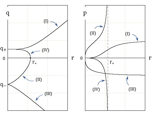
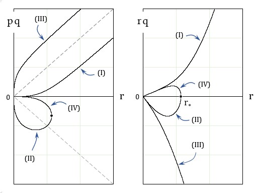
Figure 3: Plots of $q$, $p$, $pq$ and $rq$ as functions of $r$. Plots are for $r_{\text{s}}=1,\ k=r_{\text{s}}$. The leftmost panel reveals the multi-valuedness problem for $q(r)$.

The generic Buchdahl-inspired metric (1) is expressed in terms of the Schwarzschild coordinate system, $(t,r,\theta,\phi).$ This system would be problematic for metric (25)–(28) however, as we shall see below.

Despite Lemma 1 yielding the relation $r(q)$, the inversion operation to express $q$ in terms of $r$ using elementary functions cannot be carried out. The reason is that the two exponents, $\frac{q_{+}}{q_{+}-q_{-}}$ and $\frac{q_{-}}{q_{+}-q_{-}}$, in (6) are “out of sync” with each other. This trouble is further complicated by the multi-valuedness of $q(r)$.

To see the multi-valuedness problem, we shall re-plot Fig. 2 but with a small twist; we shall re-plot it against the variable $r$ in place of $q$. In Fig. 3 we plot $q$, $p$, $pq$ and $rq$ as functions of $r$; again, with $k=r_{\text{s}}=1$, $q_{+}=1/2$, $q_{-}=-3/2$, and $r_{*}:=\left|q_{+}\right|^{\frac{q_{+}}{q_{+}-q_{-}}}\left|q_{-}\right|^{-\frac{q_{-}}{q_{+}-q_{-}}}=(27)^{1/4}/2\approx 1.14$. The quadrant labels (I), (II), (III) and (IV) defined from Fig. 2 are carried over to Fig. 3; see Remark 4. In the leftmost panel of Fig. 3, the function $q(r)$ is double-valued for $r>r_{*}$, and quadruple-valued for $r<r_{*}$. This is the multi-valuedness problem which further handicaps the inversion of $q$ in terms of $r$.

The multi-valuedness means that $r$, despite playing the Schwarzschild radial coordinate in metric (1)–(3), is not a suitable variable for metric (25)–(27). However, looking back at Fig. 2, we immediately realize that the variable $q$ can be a suitable coordinate because all other variables – viz. $r$, $p$ and others – are single-valued functions of $q$. This observation guides us to the first change of variable in the next section.

II.3 A first change of variable

Corollary 9.

The special Buchdahl-inspired metric is fully analytic with respect to the variable $q$, per

$$ds^{2} =e^{\omega(q)}\biggl{\{}-\frac{p(q)\,q}{r(q)}dt^{2}+\frac{r(q)}{p(q)\,q}dq^{2}+r^{2}(q)d\Omega^{2}\biggr{\}}$$ (34)

$$r(q) =\left|q-q_{+}\right|^{\frac{q_{+}}{q_{+}-q_{-}}}\left|q-q_{-}\right|^{\frac{q_{-}}{q_{-}-q_{+}}}$$ (35)

$$\frac{q\,p(q)}{r(q)} =\text{sgn}\left(\frac{q-q_{+}}{q-q_{-}}\right)\left|\frac{q-q_{+}}{q-q_{-}}\right|^{\frac{r_{\text{s}}}{q_{+}-q_{-}}}$$ (36)

$$e^{\omega(q)} =\left|\frac{q-q_{+}}{q-q_{-}}\right|^{\frac{k}{q_{+}-q_{-}}}$$ (37)

$$k =\left(-\frac{4}{3}q_{+}q_{-}\right)^{1/2}$$ (38)

Proof.

Eq. (11) gives

$$dr=\frac{dq}{p}$$ (39)

from which, we deduce that

$$\frac{pr}{q}\,dr^{2}=\frac{r}{p\,q}\,dq^{2}$$ (40)

Metric (25) thus can be brought into (34), with the conformal factor

$$e^{\omega(q)}:=e^{k\int\frac{dr}{r\,q(r)}}=e^{k\int\frac{dq}{p(q)r(q)q}}$$ (41)

which by combining with Eqs. (27), produces Eq. (37), per

$$e^{\omega(q)}=e^{k\int\frac{dq}{(q-q_{+})(q-q_{-})}}=\left|\frac{q-q_{+}}{q-q_{-}}\right|^{\frac{k}{q_{+}-q_{-}}}$$ (42)

Also from Eq. (27)

$$\frac{q\,p}{r}=\frac{(q-q_{+})(q-q_{-})}{r^{2}}$$ (43)

and, by using Eq. (26) and noting that $q_{+}+q_{-}=r_{\text{s}}$ by virtue of (8), we arrive at Eq. (36). ∎

Remark 10.

An immediate improvement of metric (34) over metric (25) is that, apart from the conformal factor, the two components $g_{00}$ and $g_{11}$ are reciprocal of each other. This feature resembles that in the Schwarzschild metric.

II.4 A second change of variable

Despite getting a step closer to the form of a Schwarzschild metric (see Remark 10 above), the term $pq/r$ in metric (34) is still rather cumbersome; see Eq. (36). It is thus desirable to find a more transparent alternative to the coordinate $q$. The lower right panel in Fig. 2 suggests a further improvement. Not only is the combination $pq/r$ a single-valued function of $q$, the reverse is also true: $q$ is a single-valued function of $pq/r$. We shall thus choose $pq/r$ as the radial coordinate in replacement of $q$.

That is to say, let us define a new radial coordinate $\rho\in\mathbb{R}$ such that

$$1-\frac{r_{\text{s}}}{\rho}:=\frac{p(q)\,q}{r(q)}$$ (44)

which, by way of (36), becomes

$$1-\frac{r_{\text{s}}}{\rho}=\text{sgn}\left(\frac{q-q_{+}}{q-q_{-}}\right)\left|\frac{q-q_{+}}{q-q_{-}}\right|^{\frac{r_{\text{s}}}{q_{+}-q_{-}}}$$ (45)

Remarkably, despite that $q$ is not analytically expressible in terms of $r$ – a serious hindrance that we alluded to at the beginning of Sec. II.2 – the relation (45) can be inverted to express $q$ as a analytical function of $\rho$. Furthermore, since $r$ is an analytical function of $\rho$ per (35), $r$ in turn can be made an analytical function of $\rho$. The inversion of Eq. (45) shall be carried out in the following Lemma.

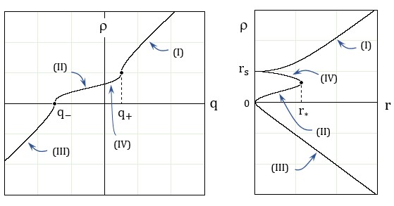
Figure 4: $\rho$ as functions of $q$ and $r$. Plots are for $r_{\text{s}}=1,\ k=r_{\text{s}}$.

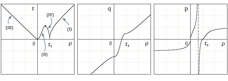
Figure 5: Various variables as functions of $\rho$. Plots are for $r_{\text{s}}=1,\ k=r_{\text{s}}$.

Lemma 11.

The Schwarzschild coordinate $r$ is expressible in terms of the variable $\rho$, per

$$r(\rho) =\frac{\zeta\,r_{\text{s}}\left|1-\frac{r_{\text{s}}}{\rho}\right|^{\frac{1}{2}\left(\zeta-1\right)}}{\left|1-\text{\emph{sgn}}\left(1-\frac{r_{\text{s}}}{\rho}\right)\left|1-\frac{r_{\text{s}}}{\rho}\right|^{\zeta}\right|}$$ (46)

$$\zeta :=\sqrt{1+3k^{2}/r_{\text{s}}^{2}}$$ (47)

Proof.

Denote:

$$x:=1-\frac{r_{\text{s}}}{\rho}$$ (48)

then, from (45)

$$x=\text{sgn}\frac{q-q_{+}}{q-q_{-}}\left|\frac{q-q_{+}}{q-q_{-}}\right|^{\frac{r_{\text{s}}}{q_{+}-q_{-}}}$$ (49)

Further define $\zeta:=\sqrt{1+3k^{2}/r_{\text{s}}^{2}}\geqslant 1\ \ \forall k\in\mathbb{R}$, then from the definition of $q_{\pm}$ in (8) we get

$$\frac{r_{\text{s}}}{q_{+}-q_{-}}=\frac{r_{\text{s}}}{\sqrt{r_{\text{s}}^{2}+3k^{2}}}=\frac{1}{\zeta}$$ (50)

Case 1:   For $q>q_{+}$ then $0<x<1$.

Inverting Eq. (49):

$$\left(\frac{q-q_{+}}{q-q_{-}}\right)^{1/\zeta} =x=\left|x\right|$$ (51)

$$q =\frac{1}{1-\left|x\right|^{\zeta}}q_{+}-\frac{\left|x\right|^{\zeta}}{1-\left|x\right|^{\zeta}}q_{-}$$ (52)

then

$$q-q_{+} =\frac{\left|x\right|^{\zeta}}{1-\left|x\right|^{\zeta}}(q_{+}-q_{-})$$ (53)

$$q-q_{-} =\frac{1}{1-\left|x\right|^{\zeta}}(q_{+}-q_{-})$$ (54)

and

$$r =(q-q_{+})^{\frac{q_{+}}{q_{+}-q_{-}}}(q-q_{-})^{-\frac{q_{-}}{q_{+}-q_{-}}}$$ (55)

$$=\left(\frac{\left|x\right|^{\zeta}}{1-\left|x\right|^{\zeta}}\right)^{\frac{q_{+}}{q_{+}-q_{-}}}\left(\frac{1}{1-\left|x\right|^{\zeta}}\right)^{-\frac{q_{-}}{q_{+}-q_{-}}}(q_{+}-q_{-})$$ (56)

$$=\frac{\left|x\right|^{\zeta\frac{1}{\sqrt{r_{\text{s}}^{2}+3k^{2}}}\frac{1}{2}\left(-r_{\text{s}}+\sqrt{r_{\text{s}}^{2}+3k^{2}}\right)}}{1-\left|x\right|^{\zeta}}\,\zeta r_{\text{s}}$$ (57)

$$=\zeta r_{\text{s}}\frac{\left|x\right|^{\frac{1}{2}(\zeta-1)}}{1-\left|x\right|^{\zeta}}$$ (58)

Case 2:   For $q<q_{-}$ then $x>1$.

Inverting Eq. (49):

$$\left(\frac{q-q_{+}}{q-q_{-}}\right)^{1/\zeta} =x=\left|x\right|$$ (59)

$$q =\frac{1}{1-\left|x\right|^{\zeta}}q_{+}-\frac{\left|x\right|^{\zeta}}{1-\left|x\right|^{\zeta}}q_{-}$$ (60)

then

$$q-q_{+} =\frac{\left|x\right|^{\zeta}}{1-\left|x\right|^{\zeta}}(q_{+}-q_{-})$$ (61)

$$q-q_{-} =\frac{1}{1-\left|x\right|^{\zeta}}(q_{+}-q_{-})$$ (62)

and

$$r =(q_{+}-q)^{\frac{q_{+}}{q_{+}-q_{-}}}(q_{-}-q)^{-\frac{q_{-}}{q_{+}-q_{-}}}$$ (63)

$$=\left(\frac{\left|x\right|^{\zeta}}{\left|1-\left|x\right|^{\zeta}\right|}\right)^{\frac{q_{+}}{q_{+}-q_{-}}}\left(\frac{1}{\left|1-\left|x\right|^{\zeta}\right|}\right)^{-\frac{q_{-}}{q_{+}-q_{-}}}(q_{+}-q_{-})$$ (64)

$$=\frac{\left|x\right|^{\zeta\frac{1}{\sqrt{r_{\text{s}}^{2}+3k^{2}}}\frac{1}{2}\left(-r_{\text{s}}+\sqrt{r_{\text{s}}^{2}+3k^{2}}\right)}}{\left|1-\left|x\right|^{\zeta}\right|}\,\zeta r_{\text{s}}$$ (65)

$$=\zeta r_{\text{s}}\frac{\left|x\right|^{\frac{1}{2}(\zeta-1)}}{\left|1-\left|x\right|^{\zeta}\right|}$$ (66)

Case 3:   For $q_{-}<q<q_{+}$ then $x<0$.

Inverting Eq. (49):

$$\left(\frac{q-q_{+}}{q_{-}-q}\right)^{1/\zeta} =-x=\left|x\right|$$ (67)

$$q =\frac{1}{1+\left|x\right|^{\zeta}}q_{+}+\frac{\left|x\right|^{\zeta}}{1+\left|x\right|^{\zeta}}q_{-}$$ (68)

then

$$q-q_{+} =-\frac{\left|x\right|^{\zeta}}{1+\left|x\right|^{\zeta}}(q_{+}-q_{-})$$ (69)

$$q-q_{-} =\frac{1}{1+\left|x\right|^{\zeta}}(q_{+}-q_{-})$$ (70)

and

$$r =(q_{+}-q)^{\frac{q_{+}}{q_{+}-q_{-}}}(q-q_{-})^{-\frac{q_{-}}{q_{+}-q_{-}}}$$ (71)

$$=\left(\frac{\left|x\right|^{\zeta}}{1+\left|x\right|^{\zeta}}\right)^{\frac{q_{+}}{q_{+}-q_{-}}}\left(\frac{1}{1+\left|x\right|^{\zeta}}\right)^{-\frac{q_{-}}{q_{+}-q_{-}}}(q_{+}-q_{-})$$ (72)

$$=\frac{\left|x\right|^{\zeta\frac{1}{\sqrt{r_{\text{s}}^{2}+3k^{2}}}\frac{1}{2}\left(-r_{\text{s}}+\sqrt{r_{\text{s}}^{2}+3k^{2}}\right)}}{1+\left|x\right|^{\zeta}}\,\zeta r_{\text{s}}$$ (73)

$$=\zeta r_{\text{s}}\frac{\left|x\right|^{\frac{1}{2}(\zeta-1)}}{1+\left|x\right|^{\zeta}}$$ (74)

In all cases, we have

$$r=\zeta\,r_{\text{s}}\frac{\left|x\right|^{\frac{1}{2}(\zeta-1)}}{\left|1-\text{sgn}(x)\left|x\right|^{\zeta}\right|}$$ (75)

which is the desired result, Eq. (46). ∎

Remark 12.

For illustration, in Fig. 4, we plot the new variable $\rho$ against $q$ and $r$. In Fig. 5, $r$, $q$ and $p$ are plotted against $\rho$. In these figures, $k=r_{\text{s}}=1$. The quadrant labels are attached accordingly.

II.5 The special Buchdahl-inspired metric

We are now ready for the final step of our derivation. The Buchdahl-inspired metric with $\Lambda=0$ is provided in Lemma 13 below.

Lemma 13.

The special Buchdahl-inspired metric is characterized by 2 parameters, $r_{\text{s}}$ and $\tilde{k}$:

$$ds^{2} =\left|1-\frac{r_{\text{s}}}{\rho}\right|^{\tilde{k}}\Biggl{\{}-\left(1-\frac{r_{\text{s}}}{\rho}\right)dt^{2}+\left(1-\frac{r_{\text{s}}}{\rho}\right)^{-1}\frac{r^{4}(\rho)}{\rho^{4}}\,d\rho^{2}$$

$$\ \ \ \ \ \ \ \ \ \ \ \ \ \ \ +r^{2}(\rho)\left(d\theta^{2}+\sin^{2}\theta d\phi^{2}\right)\Biggr{\}}$$ (76)

in which the Schwarzschild radial coordinate $r$ is related to the new radial coordinate $\rho$ per

$$r(\rho) :=\frac{\zeta\,r_{\text{s}}\left|1-\frac{r_{\text{s}}}{\rho}\right|^{\frac{1}{2}(\zeta-1)}}{\left|1-\text{\emph{sgn}}\left(1-\frac{r_{\text{s}}}{\rho}\right)\left|1-\frac{r_{\text{s}}}{\rho}\right|^{\zeta}\right|}$$ (77)

$$\zeta :=\sqrt{1+3\tilde{k}^{2}}$$ (78)

Proof.

Firstly, Eq. (45) leads to

$$\left|1-\frac{r_{\text{s}}}{\rho}\right|=\left|\frac{q-q_{+}}{q-q_{-}}\right|^{\frac{r_{\text{s}}}{q_{+}-q_{-}}}$$ (79)

which neatly brings the conformal factor (37) to

$$e^{\omega(\rho)}=\left|1-\frac{r_{\text{s}}}{\rho}\right|^{\frac{k}{r_{\text{s}}}}$$ (80)

Secondly, Eq. (79) is equivalent to

$$\ln\left|1-\frac{r_{\text{s}}}{\rho}\right|=\frac{r_{\text{s}}}{q_{+}-q_{-}}\ln\left|\frac{q-q_{+}}{q-q_{-}}\right|$$ (81)

Taking derivative on both sides of this equation:

$$\left(1-\frac{r_{\text{s}}}{\rho}\right)^{-1}\frac{r_{\text{s}}}{\rho^{2}}\,d\rho=\frac{r_{\text{s}}}{(q-q_{+})(q-q_{-})}\,dq$$ (82)

which, with the aid of Eqs. (35), (79) and $r_{\text{s}}=-\left(q_{+}+q_{-}\right)$ per (8), yields

$$dq^{2} =\left|\frac{q-q_{+}}{q-q_{-}}\right|^{-\frac{2r_{\text{s}}}{q_{+}-q_{-}}}(q-q_{+})^{2}(q-q_{-})^{2}\frac{d\rho^{2}}{\rho^{4}}$$ (83)

$$=\left|q-q_{+}\right|^{\frac{4q_{+}}{q_{+}-q_{-}}}\left|q-q_{-}\right|^{-\frac{4q_{-}}{q_{+}-q_{-}}}\frac{d\rho^{2}}{\rho^{4}}$$ (84)

$$=r^{4}(q)\frac{d\rho^{2}}{\rho^{4}}$$ (85)

Finally, by defining $\tilde{k}:=k/r_{\text{s}}$ and using (44) and (85), the components in metric (34) become

$$g_{tt} =-e^{\omega}\frac{p\,q}{r}=-\left|1-\frac{r_{\text{s}}}{\rho}\right|^{\tilde{k}}\left(1-\frac{r_{\text{s}}}{\rho}\right)$$ (86)

$$g_{\rho\rho} =g_{qq}\frac{dq^{2}}{d\rho^{2}}=e^{\omega}\frac{r}{p\,q}\frac{r^{4}}{\rho^{4}}=\left|1-\frac{r_{\text{s}}}{\rho}\right|^{\tilde{k}}\frac{1}{1-\frac{r_{\text{s}}}{\rho}}\frac{r^{4}}{\rho^{4}}$$ (87)

$$g_{\theta\theta} =e^{\omega}\,r^{2}=\left|1-\frac{r_{\text{s}}}{\rho}\right|^{\tilde{k}}r^{2}$$ (88)

$$g_{\phi\phi} =g_{\theta\theta}\,\sin^{2}\theta$$ (89)

∎

Remark 14.

The rescaled Buchdahl parameter

$$\tilde{k}:=\frac{k}{r_{\text{s}}}$$ (90)

is a dimensionless ratio.

Remark 15.

At $\tilde{k}=0$, Eqs. (77) and (78) yield $\zeta=1$ and $r(\rho)\equiv\rho$. The recovery of the Schwarzschild metric from metric (76) is obvious.

Remark 16.

The combination $1-\frac{r_{\text{s}}}{\rho}$ is universal in the special Buchdahl-inspired metric, (76)–(78), as it is in the classic Schwarzschild metric. The $g_{tt}$ component flips sign when $\rho$ varies across $r_{\text{s}}$. The radius $r_{\text{s}}$ plays the role of the “Schwarzschild” radius for pure $\mathcal{R}^{2}$ spacetime structures.

Remark 17.

In metric (76)–(78), the radial coordinate is $\rho$ and the physical “origin” is located at $\rho=0$. The usual Schwarzschild coordinate $r(\rho)$ is not the radial coordinate for this metric. Rather, apart from the conformal factor $\left|1-\frac{r_{\text{s}}}{\rho}\right|^{\tilde{k}}$, it acts as an areal coordinate via the term $r^{2}(\rho)\left[d\theta^{2}+\sin^{2}\theta d\phi^{2}\right]$ in (76).

Remark 18.

As $\rho\rightarrow\infty$, per (77) we have $r(\rho)\simeq\rho$. Metric (76) asymptotically is

$$\left|1-\frac{r_{\text{s}}}{\rho}\right|^{\tilde{k}}\biggl{\{}-\Bigl{(}1-\frac{r_{\text{s}}}{\rho}\Bigr{)}dt^{2}+\frac{r^{4}(\rho)\,d\rho^{2}}{\rho^{4}\Bigl{(}1-\frac{r_{\text{s}}}{\rho}\Bigr{)}}+r^{2}(\rho)d\Omega^{2}\biggr{\}}$$ (91)

We thus do not obtain a Schwarzschild spacetime but a conformally Schwarzschild spacetime, with the conformal factor being $\left|1-\frac{r_{\text{s}}}{\rho}\right|^{\tilde{k}}$. In principle, the effects of $\tilde{k}$ should manifest via its influence on the orbital motion of the massive objects, though not that of light.

Remark 19.

In (91), since $\left|1-\frac{r_{\text{s}}}{\rho}\right|^{\tilde{k}}\rightarrow 1$ when $r\rightarrow\infty$, the special Buchdahl-inspired metric is asymptotically flat. It can also be verified to be Ricci-scalar-flat but not Ricci flat. Its 4 non-vanishing Ricci tensor components are:

$$\mathcal{R}_{tt} =\frac{\tilde{k}(\tilde{k}+1)}{2\zeta^{4}}\left|x\right|^{2-2\zeta}\left(1-\text{sgn}(x)\left|x\right|^{\zeta}\right)^{4}$$ (92)

$$\mathcal{R}_{\rho\rho} =\frac{\tilde{k}}{2\rho^{4}\left|x\right|^{2}}\left[3\tilde{k}-1+2\zeta\frac{1+\text{sgn}(x)\left|x\right|^{\zeta}}{1-\text{sgn}(x)\left|x\right|^{\zeta}}\right]$$ (93)

$$\mathcal{R}_{\theta\theta} =\frac{\tilde{k}}{2\zeta^{2}}\left(1-\text{sgn}(x)\left|x\right|^{-\zeta}\right)\times$$

$$\left[(k-1)\left(1-\text{sgn}(x)\left|x\right|^{\zeta}\right)+\zeta\left(1+\text{sgn}(x)\left|x\right|^{\zeta}\right)\right]$$ (94)

$$\mathcal{R}_{\phi\phi} =\mathcal{R}_{\theta\theta}\sin^{2}\theta$$ (95)

in which $x:=1-\frac{r_{\text{s}}}{\rho}$, $\zeta:=\sqrt{1+3\tilde{k}^{2}}$.

In closing of this main section, Lemma 13 is the central result of our paper. With this exact analytical result, we are now well equipped to study the interior-exterior boundary and the causal structure of $\mathcal{R}^{2}$ spacetime structures in the rest of our paper.

III Application I:   Anomalous behavior of interior/exterior boundary in $\mathcal{R}^{2}$ spacetime

This section explores and reports a number of novel surprising properties of the interior-exterior boundary of $\mathcal{R}^{2}$ spacetime, described by the special Buchdahl-inspired metric attained in Lemma 13.

Metric (76)–(78) bears an interesting resemblance to the Schwarzschild metric, with four departures:

• The conformal factor, $\left|1-\frac{r_{\text{s}}}{\rho}\right|^{\tilde{k}}$;

• The $g_{\rho\rho}$ component contains the ratio $\frac{r^{4}(\rho)}{\rho^{4}}$;

• The angular part involves $r^{2}(\rho)$ instead of $\rho^{2}$.

• The function $r(\rho)$ involves the signum function $\text{sgn}\left(1-\frac{r_{\text{s}}}{\rho}\right)$, thus comprising two distinct expressions, one for $\rho<r_{\text{s}}$ and other for $\rho>r_{\text{s}}$.

Across $\rho=r_{\text{s}}$, the components $g_{00}$ and $g_{11}$ flip their signs, hence indicating an “exterior” region for $\rho\in(r_{\text{s}},+\infty)$ and an “interior” region for $\rho\in(0,r_{\text{s}})$. The nature of the interior-exterior boundary can be deduced from the $\zeta-$Kruskal-Szekeres diagram constructed in Section IV.4. In Fig. 13, the boundary for $\tilde{k}\neq 0$ (viz., $\zeta>1$) is the four hyperbolic branches surrounding Region (VI); the $\rho=r_{\text{s}}$ boundary is not a null surface in this situation. For $\tilde{k}=0$, the four hyperbolic branches degenerate into two straight lines $T=\pm X$ that are null surfaces, making the $\rho=r_{\text{s}}$ boundary the usual Schwarzschild horizon. For all values of $\tilde{k}\in\mathbb{R}$, Regions (II) and (IV) in Fig. 13 represent “interior” sections of an $\mathcal{R}^{2}$ spacetime.

III.1 Behavior of the areal radial coordinate in pure $\mathcal{R}^{2}$ gravity

We first start with the areal coordinate $r(\rho)$ as a function of the new radial coordinate $\rho$. The relation is given in Eqs. (77)–(78). The plot of $r(\rho)$ is shown in Fig. 6 for various values of $\tilde{k}$. In each panel, the curve is juxtaposed against the benchmark $r(\rho)=\rho$ diagonal (dotted) line which corresponds to the case $\tilde{k}=0$ (viz. $\zeta=\sqrt{1+3\tilde{k}^{2}}=1$).

The asymptotics:

• As $\rho\rightarrow 0$,

  $$r(\rho)\simeq\zeta r_{\text{s}}^{\frac{1}{2}(1-\zeta)}\rho^{\frac{1}{2}(\zeta+1)}\rightarrow 0\ \ \ \ \ \forall\tilde{k}$$ (96)

• As $\rho\rightarrow\infty$, the areal coordinate is asymptotically

  $$r(\rho)\simeq\rho-\frac{k^{2}r_{\text{s}}^{2}}{8\,\rho}$$ (97)

• As $\rho\rightarrow r_{\text{s}}$, for $\tilde{k}\neq 0$, $\zeta$ is strictly greater than 1 and $r(\rho)\simeq\zeta r_{\text{s}}\left|1-\frac{r_{\text{s}}}{\rho}\right|^{\frac{1}{2}\left(\zeta-1\right)}\rightarrow 0$. All curves with $\tilde{k}\neq 0$ have a zero at $\rho=r_{\text{s}}$ that separates the interior region, $\rho<r_{\text{s}}$, from the exterior region, $\rho>r_{\text{s}}$.

The fact that the areal coordinate $r(\rho)$ shrinks to zero on the interior-exterior boundary if $\tilde{k}\neq 0$ is a novel feature of pure $\mathcal{R}^{2}$ spacetime structures.

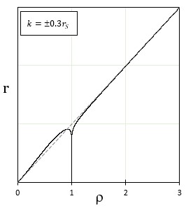
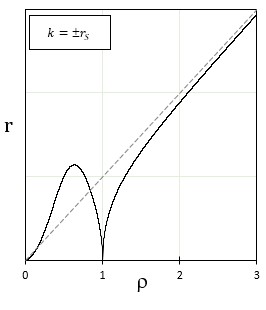
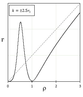
Figure 6: Areal coordinate $r$ as function of the new coordinate $\rho$. For $\tilde{k}=\pm 0.3,\pm 1,\pm 2.5$. In all plots, $r_{\text{s}}=1$.

III.2 Determinant of the metric

We next look into the determinant of metric (76)–(78),

$$-\det g =\left|1-\frac{r_{\text{s}}}{\rho}\right|^{4\tilde{k}}\frac{r^{8}(\rho)}{\rho^{4}}\,\sin^{2}\theta$$ (98)

$$=\frac{\zeta^{8}r_{\text{s}}^{8}}{\rho^{4}}\frac{\left|1-\frac{r_{\text{s}}}{\rho}\right|^{4(\zeta+\tilde{k}-1)}\,\sin^{2}\theta}{\left(1\mp\left|1-\frac{r_{\text{s}}}{\rho}\right|^{\zeta}\right)^{8}}$$ (99)

with $\mp$ corresponding the exterior/interior regions, respectively. Fig. 7 depicts a number of combinations of $\tilde{k}$ and $\zeta$ to be encountered in this paper. We deduce that

$$\zeta+\tilde{k}-1=\begin{cases}0&\text{if }\tilde{k}=0\text{ or }\tilde{k}=-1\\ >0&\text{if }\tilde{k}\in(-\infty,-1)\cup(0,+\infty)\\ <0&\text{if }\tilde{k}\in(-1,0)\end{cases}$$ (100)

Figure 7: Various combinations of $\tilde{k}$ and $\zeta$, to be used in this paper, as functions of $\tilde{k}$.

Special cases:

• At $\tilde{k}=0$:

  $$-\det g=\rho^{4}\sin^{2}\theta$$ (101)

  which is a result known in the Schwarzschild metric.

• At $\tilde{k}=-1$:

  $$-\det g=\frac{256\,r_{\text{s}}^{8}\,\sin^{2}\theta}{\rho^{4}\left(1\mp\left(1-\frac{r_{\text{s}}}{\rho}\right)^{2}\right)^{8}}$$ (102)

  with $\mp$ corresponding the exterior/interior regions, respectively. The determinant with $\tilde{k}=-1$ is well-behaved for all $\rho\neq 0$.

The asymptotic at the interior-exterior boundary, $\rho\rightarrow r_{\text{s}}$:

Due to result (100), we then have

$$\lim_{\rho\rightarrow r_{\text{s}}}\Bigl{(}-\det g|_{\theta=\frac{\pi}{2}}\Bigr{)}^{\frac{1}{4}}=\begin{cases}\ r_{\text{s}}&\text{for }\tilde{k}=0\\ \ 4\,r_{\text{s}}&\text{for }\tilde{k}=-1\\ \ 0&\text{for }\tilde{k}\leqslant-1\text{ or }\tilde{k}\geqslant 0\\ \ +\infty&\text{for $\tilde{k}\in(-1,0)$}\end{cases}$$ (103)

III.3 The Kretschmann invariant

The Kretschmann scalar is given by

$$K :=\mathcal{R}^{\mu\nu\rho\sigma}\mathcal{R}_{\mu\nu\rho\sigma}$$ (104)

$$=\frac{2}{\zeta^{8}r_{\text{s}}^{4}}\left(1-\text{sgn}(x)\left|x\right|^{\zeta}\right)^{6}\left|x\right|^{2-4\zeta-2\tilde{k}}\times$$

$$\biggl{\{}4\tilde{k}^{2}(\tilde{k}+1)\,\text{sgn}(x)\left|x\right|^{\zeta}+\zeta\,\Bigl{(}4\tilde{k}^{3}-5\tilde{k}^{2}-3\Bigr{)}\Bigl{(}1-\left|x\right|^{2\zeta}\Bigr{)}$$

$$+\Bigl{(}9\tilde{k}^{4}-2\tilde{k}^{3}+10\tilde{k}^{2}+3\Bigr{)}\Bigl{(}1+\left|x\right|^{2\zeta}\Bigr{)}\biggr{\}}$$ (105)

in which $x:=1-\frac{r_{\text{s}}}{\rho}$.

By completing the square in the curly bracket in expression (105) in terms of $\left|x\right|^{\zeta}$, one can show that the Kretschmann scalar is positive-definite for all $\rho\in\mathbb{R}$ and all $k\in\mathbb{R}$.

Special cases:

• At $\tilde{k}=0$, i.e. $\zeta=1$

  $$K=\frac{12r_{\text{s}}^{2}}{\rho^{6}}$$ (106)

  recovering the result known in the Schwarzschild metric. It only has a curvature singularity at the origin.

• At $\tilde{k}=-1$, i.e. $\zeta=2$

  $$K=\frac{3}{8r_{\text{s}}^{4}}\left(1\mp\left(1-\frac{r_{\text{s}}}{\rho}\right)^{2}\right)^{6}$$ (107)

  with $\mp$ corresponding to the exterior/interior regions, respectively. It also only has a curvature singularity at the origin.

The asymptotics:

• As $\rho\rightarrow+\infty$, viz. $x\rightarrow 1$,

  $$K \simeq\frac{12}{\zeta^{8}r_{\text{s}}^{4}}\Bigl{(}\tilde{k}^{2}+1\Bigr{)}\Bigl{(}3\tilde{k}^{2}+1\Bigr{)}\left(1-\left|1-\frac{r_{\text{s}}}{\rho}\right|^{\zeta}\right)^{6}$$ (108)

  $$\simeq 12\Bigl{(}\tilde{k}^{2}+1\Bigr{)}\frac{r_{\text{s}}^{2}}{\rho^{6}}$$ (109)

  which decays as $\rho^{-6}$ when $\rho\rightarrow+\infty$ for $\forall\tilde{k}\in\mathbb{R}$.

• As $\rho\rightarrow 0$, viz. $x\rightarrow\infty$,

  $$K \simeq\frac{2}{\zeta^{8}r_{\text{s}}^{4}}\left|x\right|^{2\zeta-2\tilde{k}+2}\Biggl{\{}4\tilde{k}^{2}\left(\tilde{k}+1\right)\left|x\right|^{\zeta}+$$

  $$\left[\left(-4\tilde{k}^{3}+5\tilde{k}^{2}+3\right)\zeta+\left(9\tilde{k}^{4}-2\tilde{k}^{3}+10\tilde{k}^{2}+3\right)\right]\left|x\right|^{2\zeta}\Biggr{\}}$$ (110)

  Since $\zeta=\left(1+3\tilde{k}^{2}\right)^{\frac{1}{2}}\geqslant 1$ for $\forall\tilde{k}\in\mathbb{R}$, $\left|x\right|^{2\zeta}$ dominates $\left|x\right|^{\zeta}$ as $x\rightarrow\infty$. Hence, as $\rho\rightarrow 0$,

  $$K\simeq\frac{2}{\zeta^{8}r_{\text{s}}^{4}}\left(\frac{r_{\text{s}}}{\rho}\right)^{2\left(2\zeta-\tilde{k}+1\right)}\times$$

  $$\left[\left(-4\tilde{k}^{3}+5\tilde{k}^{2}+3\right)\zeta+\left(9\tilde{k}^{4}-2\tilde{k}^{3}+10\tilde{k}^{2}+3\right)\right]$$ (111)

  From Fig. 7, $2\zeta-\tilde{k}+1>0\ \ \forall\tilde{k}\in\mathbb{R}$. Thus $K$ diverges as $\rho^{-2\left(2\zeta-\tilde{k}+1\right)}$ when $\rho\rightarrow 0$, for all $\forall\tilde{k}\in\mathbb{R}$.

• As $\rho\rightarrow r_{\text{s}}$, viz. $x\rightarrow 0$, if $\tilde{k}\neq 0$ and $\tilde{k}\neq-1$

  $$K\simeq\frac{2}{\zeta^{8}r_{\text{s}}^{4}}\left|1-\frac{r_{\text{s}}}{\rho}\right|^{2\left(-2\zeta-\tilde{k}+1\right)}\times$$

  $$\left[\left(4\tilde{k}^{3}-5\tilde{k}^{2}-3\right)\zeta+\left(9\tilde{k}^{4}-2\tilde{k}^{3}+10\tilde{k}^{2}+3\right)\right]$$ (112)

  From Fig. 7, $-2\zeta-\tilde{k}+1<0\ \ \forall k\in\mathbb{R}.$ Thus $K$ diverges as $\left|\rho-r_{\text{s}}\right|^{2\left(-2\zeta-\tilde{k}+1\right)}$ when $\rho\rightarrow r_{\text{s}}$, for $\tilde{k}\neq 0$ and $\tilde{k}\neq-1$. In sum, when $\rho\rightarrow r_{\text{s}}$,

  $$K\simeq\begin{cases}\ 12\,r_{\text{s}}^{-4}&\text{for }\tilde{k}=0\\ \ \frac{3}{8}\,r_{\text{s}}^{-4}&\text{for }\tilde{k}=-1\\ \ \left|\rho-r_{\text{s}}\right|^{2\left(-2\zeta-\tilde{k}+1\right)}\rightarrow+\infty&\text{otherwise}\end{cases}$$ (113)

The fact that, for $\tilde{k}\neq 0$ and $\tilde{k}\neq-1$, the Kretschmann scalar exhibits an additional singularity on the interior-exterior boundary, $\rho=r_{\text{s}}$, besides the usual singularity at the origin, is another novel result.

The plot for the Kretschmann scalar is shown in Fig. 8. For clarity, we split the curves into two groups, one with negative $\tilde{k}$ (upper panel), the other non-negative $\tilde{k}$ (lower panel). The curves with $\tilde{k}=0$ and $\tilde{k}=-1$ are smooth across the interior-exterior boundary, $\rho=r_{\text{s}}$. All other curves show a divergence at $\rho=r_{\text{s}}$.

 

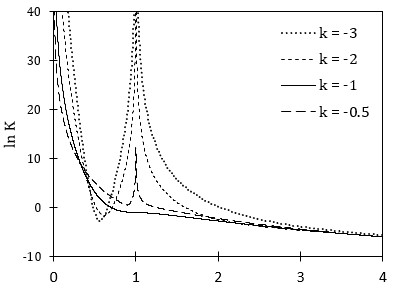
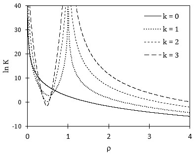
Figure 8: Logarithm of Kretschmann invariant as function of the new coordinate $\rho$, for various value of $\tilde{k}$. For clarity, we plot the curves in two panels. In all cases, $r_{\text{s}}=1$.

III.4 Surface area of the interior-exterior boundary of $\mathcal{R}^{2}$ spacetime: An anomalous behavior

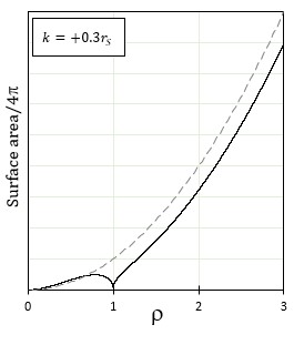
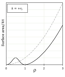
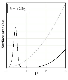
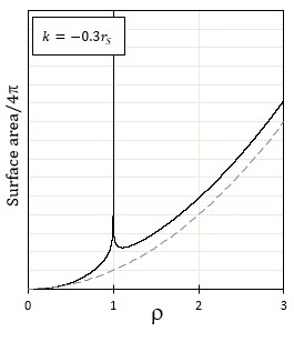
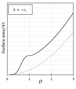
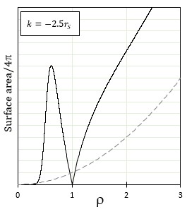
Figure 9: Surface area as function of the new coordinate $\rho$. Upper panels: $\tilde{k}=0.3,1,2.5$. Lower panels: $\tilde{k}=-0.3,-1,-2.5$. The dash line in each panel is the trivial $\tilde{k}=0$ benchmark, $A=4\pi\rho^{2}$.

For metric (76)–(77), the surface area of a two-dimensional sphere of “radius” $\rho$ is

$$A =4\pi\left|1-\frac{r_{\text{s}}}{\rho}\right|^{\tilde{k}}r^{2}(\rho)$$

$$=4\pi\zeta^{2}r_{\text{s}}^{2}\frac{\left|1-\frac{r_{\text{s}}}{\rho}\right|^{\zeta+\tilde{k}-1}}{\left(1-\text{sgn}\left(1-\frac{r_{\text{s}}}{\rho}\right)\left|1-\frac{r_{\text{s}}}{\rho}\right|^{\zeta}\right)^{2}}$$ (114)

which is conveniently equal to

$$4\pi\rho\,\biggl{(}-\det g\Bigr{|}_{\theta=\pi/2}\biggr{)}^{\frac{1}{4}}$$ (115)

The surface area $A$ and the determinant of $g$ thus share similar behaviors. The plot of $A$ is shown in Fig. 9, with the dotted parabola showing the regular $\tilde{k}=0$, in which case $A=4\pi\rho^{2}$ since $r(\rho)=\rho$. Note the plots are not symmetric with respect to $\tilde{k}$.

The asymptotics:

• As $\rho\rightarrow+\infty$,

  $$A\simeq 4\pi\Bigl{[}\rho^{2}-\tilde{k}r_{\text{s}}\rho-\frac{r_{\text{s}}^{2}}{4}\tilde{k}(\tilde{k}-2)\Bigr{]}$$ (116)

• As $\rho\rightarrow 0$,

  $$A\simeq 4\pi\zeta^{2}r_{\text{s}}^{2}\rho^{\zeta-\tilde{k}+1}$$ (117)

  From Fig. 7, $\zeta-\tilde{k}+1>0\ \ \forall\tilde{k}\in\mathbb{R}$. Hence, $A\rightarrow 0$ as $\rho\rightarrow 0$ for $\forall\tilde{k}\in\mathbb{R}$.

• As $\rho\rightarrow r_{\text{s}}$,

  $$A \simeq 4\pi\zeta^{2}r_{\text{s}}^{2}\left|1-\frac{r_{\text{s}}}{\rho}\right|^{\zeta+\tilde{k}-1}$$ (118)

  $$=\begin{cases}\ 4\pi r_{\text{s}}^{2}&\text{if }\tilde{k}=0\\ \ 16\pi r_{\text{s}}^{2}&\text{if }\tilde{k}=-1\\ \ 0&\text{if }\tilde{k}\in(-\infty,-1)\cup(0,+\infty)\\ \ \text{+$\infty$}&\text{if }\tilde{k}\in\left(-1,0)\right)\end{cases}$$ (119)

Remark 20.

Depending on the value of $\tilde{k}$, the shrinkage or divergence of the surface area at $\rho=r_{\text{s}}$ is evident in Fig. 9.

Remark 21.

The interior-exterior boundary exhibits a peculiar property. Per Eq. (119), its surface area with $\tilde{k}\neq 0$ drastically deviates from the customary $4\pi r_{\text{s}}^{2}$ expression, thereby indicating that the Buchdahl parameter $k$ “distorts” the topology of spacetime around the interior-exterior boundary.

Remark 22.

The anomalous behavior of the surface area of the interior-exterior boundary occurs in tandem with the curvature singularity at the interior-exterior boundary in the Kretschmann invariant, Eq. (113); also see Section V.0.6.

IV Application II:   Causal structure of pure $\mathcal{R}^{2}$ spacetime

This section analytically constructs the Kruskal-Szekeres (KS) diagram of the special Buchdahl-inspired metric attained in Lemma 13. We adapt the usual practices that handle Schwarzschild black holes – by finding the tortoise coordinates, the Eddington-Finkelstein coordinates, and the Kruskal-Szekeres coordinates (Eddington-1924, ; Finkelstein-1958, ; Szekeres-1960, ; Kruskal-1960, ) – to the case at hand. Quantitative adjustments are needed. With metric (76)–(78) involving the parameter $\zeta$, we shall label these said coordinates by a $\zeta-$ prefix. Fig. 13 is the outcome of our construction.

IV.1 Constructing the $\boldsymbol{\zeta-}$tortoise coordinate for pure $\mathcal{R}^{2}$ gravity

The $\zeta-$tortoise coordinate $\rho^{*}(\rho)$ is defined as

$$d\rho^{*}:=\frac{r^{2}(\rho)}{\rho^{2}(1-\frac{r_{\text{s}}}{\rho})}d\rho$$ (120)

$$d\rho^{*} =\zeta^{2}r_{\text{s}}^{2}\frac{\left|1-\frac{r_{\text{s}}}{\rho}\right|^{\zeta-1}\left(1-\frac{r_{\text{s}}}{\rho}\right)^{-1}}{\left(1-\text{sgn}(1-\frac{r_{\text{s}}}{\rho})\left|1-\frac{r_{\text{s}}}{\rho}\right|^{\zeta}\right)^{2}}\frac{d\rho}{\rho^{2}}$$ (121)

The integral involves a Gaussian hypergeometric function. Let us define

$$z:=\text{sgn}\left(1-\frac{r_{\text{s}}}{\rho}\right)\left|1-\frac{r_{\text{s}}}{\rho}\right|^{\zeta}$$ (122)

For $\rho>r_{\text{s}}$:

$$z =\left(1-\frac{r_{\text{s}}}{\rho}\right)^{\zeta}>0$$ (123)

$$dz =\zeta r_{\text{s}}\left(1-\frac{r_{\text{s}}}{\rho}\right)^{\zeta-1}\frac{d\rho}{\rho^{2}}$$ (124)

$$d\rho^{*}=\zeta r_{\text{s}}\frac{z^{-1/\zeta}}{(1-z)^{2}}dz$$ (125)

giving (modulo an additive constant)

$$\rho^{*} =\frac{\zeta^{2}r_{\text{s}}}{\zeta-1}\,z^{1-\frac{1}{\zeta}}\,_{2}F_{1}\left(2,1-\frac{1}{\zeta};2-\frac{1}{\zeta};z\right)$$ (126)

For $0<\rho<r_{\text{s}}$:

$$z =-\left(\frac{r_{\text{s}}}{\rho}-1\right)^{\zeta}<0$$ (127)

$$dz =\zeta r_{\text{s}}\left(\frac{r_{\text{s}}}{\rho}-1\right)^{\zeta-1}\frac{d\rho}{\rho^{2}}$$ (128)

$$d\rho^{*} =-\zeta r_{\text{s}}\frac{\left(-z\right)^{-1/\zeta}}{(1-z)^{2}}dz$$ (129)

$$=\zeta r_{\text{s}}\frac{\left(-z\right)^{-1/\zeta}}{(1+(-z))^{2}}d(-z)$$ (130)

giving (modulo an additive constant)

$$\rho^{*} =\frac{\zeta^{2}r_{\text{s}}}{\zeta-1}\,\left(-z\right)^{1-\frac{1}{\zeta}}\,_{2}F_{1}\left(2,1-\frac{1}{\zeta};2-\frac{1}{\zeta};z\right)$$ (131)

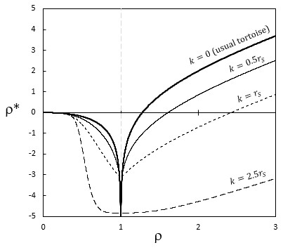
Figure 10: The $\zeta-$tortoise coordinate of Eq. (135) for various values of $\tilde{k}$ (with $r_{\text{s}}=1$).

 

Figure 11: $\rho^{*}(\rho=r_{\text{s}})$ as function of $\zeta$; both axes in log scale (with $r_{\text{s}}=1$). The two asymptopes are $\zeta/(\zeta-1)$ (for $\tilde{k}\rightarrow 0$) and $\zeta$ (for $\tilde{k}\rightarrow\infty$). Note that $\rho^{*}(\rho=r_{\text{s}})=-\pi$ for $\tilde{k}=1$.

In combination, we have the $\zeta-$tortoise coordinate (modulo an additive constant) in terms of $z\in\mathbb{C}$

$$\rho^{*} =\frac{\zeta^{2}r_{\text{s}}}{\zeta-1}\,\left|z\right|^{1-\frac{1}{\zeta}}\,_{2}F_{1}\left(2,1-\frac{1}{\zeta};2-\frac{1}{\zeta};z\right)$$ (132)

Furthermore, using Eq. (130), the difference

$$\rho^{*}|_{\rho=0}-\rho^{*}|_{\rho=r_{\text{s}}} =\int_{z=0}^{z=-\infty}\zeta r_{\text{s}}\frac{\left(-z\right)^{-1/\zeta}d(-z)}{(1+(-z))^{2}}$$ (133)

$$=\frac{\pi r_{\text{s}}}{\sin(\pi/\zeta)}$$ (134)

We shall choose the additive constant such that the $\zeta-$tortoise coordinate vanishes at $\rho=0$. Using (122) and (134), (132) produces

$$\rho^{*} =-\frac{\pi r_{\text{s}}}{\sin(\pi/\zeta)}+\frac{\zeta^{2}r_{\text{s}}}{\zeta-1}\left|1-\frac{r_{\text{s}}}{\rho}\right|^{\zeta-1}\times$$

$$\ \ \ \,{}_{2}F_{1}\left(2,1-\frac{1}{\zeta};2-\frac{1}{\zeta};\text{sgn}\left(1-\frac{r_{\text{s}}}{\rho}\right)\left|1-\frac{r_{\text{s}}}{\rho}\right|^{\zeta}\right)$$ (135)

For $\tilde{k}\neq 0$, the variable $\rho^{*}$ is continuous across $\rho=r_{\text{s}}$ and $\rho^{*}|_{\rho=r_{\text{s}}}=-\frac{\pi r_{\text{s}}}{\sin(\pi/\zeta)}$. In the complex plane $z\in\mathbb{C}$, the Gaussian hypergeometric function $\,{}_{2}F_{1}\left(2,1-1/\zeta;2-1/\zeta;z\right)$ has a branch point at $z=1$; expression (135) is thus applicable for $z\in\mathbb{R}^{+}$ and $\tilde{k}\neq 0$. See Appendix B for more information on the hypergeometric function at play.

For $\tilde{k}=0$, i.e. $\zeta=1$, the tortoise coordinate (135) duly recovers

$$\rho^{*}=\rho+r_{\text{s}}\ln\left|\frac{\rho-r_{\text{s}}}{r_{\text{s}}}\right|$$ (136)

which diverges at $\rho=r_{\text{s}}$. See Appendix C for derivation.

Fig. 10 plots the $\zeta-$tortoise coordinate for various values of $\tilde{k}$. The case of $\tilde{k}=0$ is the usual tortoise coordinate, Eq. (136). Fig. 11 shows the value $-\rho^{*}|_{\rho=r_{\text{s}}}=\frac{\pi r_{\text{s}}}{\sin(\pi/\zeta)}$ which asymptotes $\frac{\zeta r_{\text{s}}}{\zeta-1}$ for $\zeta\gtrsim 1$ and $\zeta r_{\text{s}}$ for large $\zeta$.

IV.2 Constructing the $\boldsymbol{\zeta-}$Eddington-Finkelstein coordinates for pure $\mathcal{R}^{2}$ gravity

Let us define the advanced and retarded $\zeta-$Eddington-Finkelstein coordinates, per

$$v :=t+\rho^{*}$$ (137)

$$u :=t-\rho^{*}$$ (138)

Metric (76), expressed in these new coordinates, becomes

$$ds^{2} =\left|1-\frac{r_{\text{s}}}{\rho}\right|^{\tilde{k}}\times$$

$$\biggl{\{}-\left(1-\frac{r_{\text{s}}}{\rho}\right)dv^{2}+\frac{r^{2}(\rho)}{\rho^{2}}\left(2dv\,d\rho+\rho^{2}d\Omega^{2}\right)\biggr{\}}$$ (139)

and

$$ds^{2} =\left|1-\frac{r_{\text{s}}}{\rho}\right|^{\tilde{k}}\times$$

$$\biggl{\{}-\left(1-\frac{r_{\text{s}}}{\rho}\right)du^{2}+\frac{r^{2}(\rho)}{\rho^{2}}\left(-2du\,d\rho+\rho^{2}d\Omega^{2}\right)\biggr{\}}$$ (140)

Also

$$du\,dv=dt^{2}-\frac{r^{4}(\rho)}{\rho^{4}\left(1-\frac{r_{\text{s}}}{\rho}\right)^{2}}d\rho^{2}$$ (141)

thence

$$ds^{2}=\left|1-\frac{r_{\text{s}}}{\rho}\right|^{\tilde{k}}\biggl{\{}-\left(1-\frac{r_{\text{s}}}{\rho}\right)du\,dv+r^{2}(\rho)\,d\Omega^{2}\biggr{\}}$$ (142)

In the advanced $\zeta-$Eddington-Finkelstein coordinate, the null geodesics ($ds^{2}=0$) along the radial direction amount to

$$\frac{dv}{d\rho}=\begin{cases}0&\text{(infalling)}\\ \frac{2r^{2}(\rho)}{\rho^{2}\left(1-\frac{r_{\text{s}}}{\rho}\right)}=2\frac{d\rho^{*}}{d\rho}&\text{(outgoing)}\end{cases}$$ (143)

thus

$$v=\begin{cases}\text{const}&\text{(infalling)}\\ 2\rho^{*}+\text{const}&\text{(outgoing)}\end{cases}$$ (144)

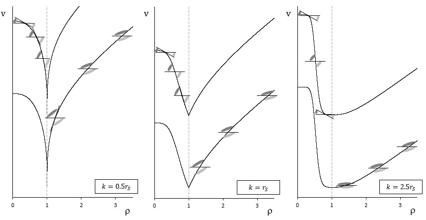
Figure 12: Light cones in the $(\rho,v)$ plane (with $r_{\text{s}}=1$), for $\tilde{k}=0.5,1,2.5$. We choose these values of $\tilde{k}$ as representatives for the three cases discussed in the text.

IV.3 Behavior of light cones across the interior-exterior boundary of a pure $\mathcal{R}^{2}$ spacetime

In the advanced $\zeta-$Eddington-Finkelstein coordinates, per (143) and (121), the outgoing null path has the slope

$$\frac{dv}{d\rho} =2\frac{d\rho^{*}}{d\rho}$$ (145)

$$=\frac{2\zeta^{2}}{1-\frac{r_{\text{s}}}{\rho}}\left(\frac{r_{\text{s}}}{\rho}\right)^{2}\frac{\left|1-\frac{r_{\text{s}}}{\rho}\right|^{\zeta-1}}{\left(1-\text{sgn}\left(1-\frac{r_{\text{s}}}{\rho}\right)\left|1-\frac{r_{\text{s}}}{\rho}\right|^{\zeta}\right)^{2}}$$ (146)

Thus the outgoing null path exhibits the following asymptotic behaviors

$$\frac{dv}{d\rho}\simeq\begin{cases}\ -2\zeta^{2}r_{\text{s}}^{2(1-\zeta)}\rho^{\zeta}\rightarrow 0&\text{as }\rho\rightarrow 0\\ \ +2\zeta^{2}r_{\text{s}}^{2-\zeta}\left|\rho-r_{\text{s}}\right|^{\zeta-2}&\text{as }\rho\rightarrow r_{\text{s}}^{+}\\ \ -2\zeta^{2}r_{\text{s}}^{2-\zeta}\left|\rho-r_{\text{s}}\right|^{\zeta-2}&\text{as }\rho\rightarrow r_{\text{s}}^{-}\\ \ +2&\text{as }\rho\rightarrow\infty\end{cases}$$ (147)

Fig. 12 depicts the behavior of the light cones in the $(v,\rho)$ plane. Concerning the light cone behavior across the interior-exterior boundary, there are three cases:

1. For $\left|\tilde{k}\right|<1$, viz. $\zeta<2$

   $$\frac{dv}{d\rho}\rightarrow\pm\infty\text{ as }\rho\rightarrow r_{\text{s}}^{\pm}$$ (148)

   The light cone “flips over” across the interior-exterior boundary as usual. This case includes the standard Schwarzschild metric, viz. $\tilde{k}=0$. See the leftmost panel in Fig. 12.

2. For $\left|\tilde{k}\right|>1$, viz. $\zeta>2$

   $$\frac{dv}{d\rho}\rightarrow 0^{\pm}\text{ as }\rho\rightarrow r_{\text{s}}^{\pm}$$ (149)

   This case is a peculiar situation. The light cone first “flattens out” when approaching the interior-exterior boundary from the exterior. Upon passing the interior-exterior boundary, the light cone makes sudden “collapse” to an single line, $dv=0$, then gradually “re-widens” when entering into the interior. See the rightmost panel in Fig. 12.

3. For $\left|\tilde{k}\right|=1$, hence $\zeta=2$

   $$\frac{dv}{d\rho}\rightarrow\pm 8\text{ as }\rho\rightarrow r_{\text{s}}^{\pm}$$ (150)

   The light cones changes its slope in a step-wise fashion. See the middle panel in Fig. 12.

Remark 23.

From Fig. 12, in every situation, all light paths and time-like paths inside the interior-exterior boundary would eventually reach the origin; they cannot escape from the interior. In the exterior region, the outgoing light path can escape to infinity. These results shall be confirmed by way of the Kruskal-Szekeres diagram in Sec. IV.4 below.

IV.4 Constructing the $\boldsymbol{\zeta-}$Kruskal-Szekeres coordinates for pure $\mathcal{R}^{2}$ gravity

Most of the procedure originally advanced by Kruskal and Szekeres for Schwarzschild black holes (Kruskal-1960, ; Szekeres-1960, ) can be re-purposed for pure $\mathcal{R}^{2}$ spacetime. We shall consider the exterior and interior regions separately.

The exterior

For $\rho>r_{\text{s}}$, let us define

$$X :=\frac{1}{2}\left(e^{\frac{v}{2r_{\text{s}}}}+e^{-\frac{u}{2r_{\text{s}}}}\right)$$ (151)

$$T :=\frac{1}{2}\left(e^{\frac{v}{2r_{\text{s}}}}-e^{-\frac{u}{2r_{\text{s}}}}\right)$$ (152)

then

$$X =e^{\frac{\rho^{*}}{2r_{\text{s}}}}\cosh\frac{t}{2r_{\text{s}}}$$ (153)

$$T =e^{\frac{\rho^{*}}{2r_{\text{s}}}}\sinh\frac{t}{2r_{\text{s}}}$$ (154)

$$T^{2}-X^{2} =-e^{\frac{\rho^{*}}{r_{\text{s}}}}$$ (155)

$$\frac{T}{X} =\tanh\frac{t}{2r_{\text{s}}}$$ (156)

and

$$dX =\frac{e^{\frac{\rho^{*}}{2r_{\text{s}}}}}{2r_{\text{s}}}\left[\frac{r^{2}(\rho)}{\rho^{2}\left(1-\frac{r_{\text{s}}}{\rho}\right)}\cosh\frac{t}{2r_{\text{s}}}d\rho+\sinh\frac{t}{2r_{\text{s}}}dt\right]$$ (157)

$$dT =\frac{e^{\frac{\rho^{*}}{2r_{\text{s}}}}}{2r_{\text{s}}}\left[\frac{r^{2}(\rho)}{\rho^{2}\left(1-\frac{r_{\text{s}}}{\rho}\right)}\sinh\frac{t}{2r_{\text{s}}}d\rho+\cosh\frac{t}{2r_{\text{s}}}dt\right]$$ (158)

hence

$$dT^{2}-dX^{2}=\frac{e^{\frac{\rho^{*}}{r_{\text{s}}}}}{4r_{\text{s}}^{2}}\left[dt^{2}-\frac{r^{4}(\rho)}{\rho^{4}\left(1-\frac{r_{\text{s}}}{\rho}\right)^{2}}d\rho^{2}\right]$$ (159)

giving

$$ds^{2} =\left|1-\frac{r_{\text{s}}}{\rho}\right|^{\tilde{k}}\times$$

$$\left\{-4r_{\text{s}}^{2}e^{-\frac{\rho^{*}}{r_{\text{s}}}}\left(1-\frac{r_{\text{s}}}{\rho}\right)\left(dT^{2}-dX^{2}\right)+r^{2}(\rho)d\Omega^{2}\right\}$$ (160)

The interior

For $\rho<r_{\text{s}}$, let us define

$$X :=\frac{1}{2}\left(e^{\frac{v}{2r_{\text{s}}}}-e^{-\frac{u}{2r_{\text{s}}}}\right)$$ (161)

$$T :=\frac{1}{2}\left(e^{\frac{v}{2r_{\text{s}}}}+e^{-\frac{u}{2r_{\text{s}}}}\right)$$ (162)

then

$$X =e^{\frac{\rho^{*}}{2r_{\text{s}}}}\sinh\frac{t}{2r_{\text{s}}}$$ (163)

$$T =e^{\frac{\rho^{*}}{2r_{\text{s}}}}\cosh\frac{t}{2r_{\text{s}}}$$ (164)

$$T^{2}-X^{2} =+e^{\frac{\rho^{*}}{r_{\text{s}}}}$$ (165)

$$\frac{T}{X} =\left(\tanh\frac{t}{2r_{\text{s}}}\right)^{-1}$$ (166)

and

$$dX =\frac{e^{\frac{\rho^{*}}{2r_{\text{s}}}}}{2r_{\text{s}}}\left[\frac{r^{2}(\rho)}{\rho^{2}\left(1-\frac{r_{\text{s}}}{\rho}\right)}\sinh\frac{t}{2r_{\text{s}}}d\rho+\cosh\frac{t}{2r_{\text{s}}}dt\right]$$ (167)

$$dT =\frac{e^{\frac{\rho^{*}}{2r_{\text{s}}}}}{2r_{\text{s}}}\left[\frac{r^{2}(\rho)}{\rho^{2}\left(1-\frac{r_{\text{s}}}{\rho}\right)}\cosh\frac{t}{2r_{\text{s}}}d\rho+\sinh\frac{t}{2r_{\text{s}}}dt\right]$$ (168)

hence

$$dT^{2}-dX^{2}=-\frac{e^{\frac{\rho^{*}}{r_{\text{s}}}}}{4r_{\text{s}}^{2}}\left[dt^{2}-\frac{r^{4}(\rho)}{\rho^{4}\left(1-\frac{r_{\text{s}}}{\rho}\right)^{2}}d\rho^{2}\right]$$ (169)

giving

$$ds^{2} =\left|1-\frac{r_{\text{s}}}{\rho}\right|^{\tilde{k}}\times$$

$$\left\{+4r_{\text{s}}^{2}e^{-\frac{\rho^{*}}{r_{\text{s}}}}\left(1-\frac{r_{\text{s}}}{\rho}\right)\left(dT^{2}-dX^{2}\right)+r^{2}(\rho)d\Omega^{2}\right\}$$ (170)

Combination of both regions

The special Buchdahl-inspired metric in the $\zeta-$Kruskal-Szekeres (KS) coordinates is thus

$$ds^{2} =\left|1-\frac{r_{\text{s}}}{\rho}\right|^{\tilde{k}}\times$$

$$\left\{-4r_{\text{s}}^{2}e^{-\frac{\rho^{*}}{r_{\text{s}}}}\left|1-\frac{r_{\text{s}}}{\rho}\right|\left(dT^{2}-dX^{2}\right)+r^{2}(\rho)d\Omega^{2}\right\}$$ (171)

and

$$T^{2}-X^{2} =-\text{sgn($\rho-r_{\text{s}})$}e^{\frac{\rho^{*}}{r_{\text{s}}}}$$ (172)

$$\frac{T}{X} =\left(\tanh\frac{t}{2r_{\text{s}}}\right)^{\text{sgn($\rho-r_{\text{s}})$}}$$ (173)

Remark 24.

For the case $\tilde{k}=0$, substituting $\rho^{*}=\rho+r_{\text{s}}\ln\left|\frac{\rho}{r_{\text{s}}}-1\right|$ and $r(\rho)=\rho$ into (171), we get

$$ds_{\text{ (KS)}}^{2}=-4r_{\text{s}}^{3}\frac{e^{-\frac{\rho}{r_{\text{s}}}}}{\rho}\left(dT^{2}-dX^{2}\right)+\rho^{2}d\Omega^{2}$$ (174)

which is the usual KS result for Schwarzschild black holes.

IV.5 Features of the $\boldsymbol{\zeta-}$Kruskal-Szekeres diagram: A new “virtual” region

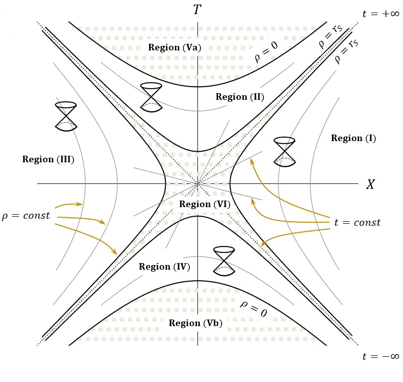
Figure 13: Kruskal-Szekeres diagram for $\tilde{k}\neq 0$. The “gulf” shown as Region (VI) is a new feature. See text for explanations.

Restricting to the radial direction, viz. $d\theta=d\phi=0$, metric (171) is

$$ds^{2}=-4r_{\text{s}}^{2}e^{-\frac{\rho^{*}}{r_{\text{s}}}}\left|1-\frac{r_{\text{s}}}{\rho}\right|^{1+\tilde{k}}\left(dT^{2}-dX^{2}\right)$$ (175)

The $\zeta-$Kruskal-Szekeres ($\zeta-$KS for short) plane for metric (175) is shown in Fig. 13. A number of key features are:

• Similarly to the usual KS diagram, the $\zeta-$KS diagram is conformally Minkowski.

• The null geodesics are:

  $$dX=\pm dT$$ (176)

  Light thus travels on the $45^{\circ}$ lines in the $\zeta-$KS plane.

• The $\zeta-$KS diagram retains, qualitatively, most features of the causal structure established for the usual KS diagram. There are quantitative changes; see below.

• A constant–$\rho$ contour corresponds to a hyperbola, whereas the constant–$t$ contour to a straight line through the origin of the $(T,X)$ plane.

• The coordinate origin $\rho=0$ amounts to, per

  $$T^{2}-X^{2}=1$$ (177)

  because $\rho^{*}(\rho=0)=0$.

• The interior-exterior boundary $\rho=r_{\text{s}}$ amounts to two distinct hyperbolae, one for the interior and the other the exterior, per

  $$T^{2}-X^{2}=\begin{cases}-e^{-\frac{\pi}{\sin\frac{\pi}{\zeta}}}&\text{for exterior}\\ +e^{-\frac{\pi}{\sin\frac{\pi}{\zeta}}}&\text{for interior}\end{cases}$$ (178)

  Note that each hyperbola comprises of two separate branches on its own.

• For $\tilde{k}=0$, viz. $\zeta=1$, the hyperbolae (178) degenerate to two straight lines

  $$T=\pm X$$ (179)

  as expected for Schwarzschild black holes.

• Region (I) is the exterior, mapped into the $\zeta-$KS plane extended up to the right branch of the hyperbola $T^{2}-X^{2}=-e^{-\frac{\pi}{\sin\frac{\pi}{\zeta}}}$.

• Region (II) is the interior, mapped into the $\zeta-$KS plane, extended up to the upper branch of the hyperbola $T^{2}-X^{2}=+e^{-\frac{\pi}{\sin\frac{\pi}{\zeta}}}$.

• Regions (III) and (IV) are time-reverse images of Regions (I) and (II).

• Regions (Va) and (Vb) (shaded by dots) are unphysical, viz. $\rho<0$.

• What is new is Region (VI) (also shaded in dots) that sandwiches between the four hyperbola branches given by (178).

In Region (II), all timelike and null trajectories will eventually hit the origin, denoted by the hyperbola, $\rho=0$. Nothing can escape from the interior. In Region (I), outgoing light paths would be able to escape to infinity. These observations are in agreement with the result obtained in Sec. IV.3; see Remark 23.

Incoming light paths from Region (I) must enter Region (II) by “bypassing” Region (VI). An infalling object (or light wave) would hit the interior-exterior boundary $\rho=r_{\text{s}}$ on the side of Region (I) then reappear on the interior-exterior boundary on the side of Region (II). The “transit” – if there is any – within Region (VI) is not visible, thus “virtual”, for an outside observer from afar.

Region (VI) appears as a “gulf” in the $(T,X)$ coordinate system but it does not correspond to any region in the $(t,\rho)$ coordinate system. When $\tilde{k}\rightarrow 0$, the “gulf” shrinks toward the 2 lines $T=\pm X$. Given that the $\zeta-$KS diagram is the maximal extension of the special Buchdahl-inspired metric, the emergence of Region (VI) is a highly curious feature, signaling potential new physics that takes place on the interior-exterior boundary of $\mathcal{R}^{2}$ spacetime. Taken altogether, the singularity on the interior-exterior boundary in the Kretschmann invariant, the anomalous behavior of the surface area of the interior-exterior boundary, and the “gulf” in the $\zeta-$KS diagram indicate that the topology of $\mathcal{R}^{2}$-gravity spacetime around a mass source undergoes fundamental alterations when the Buchdahl parameter $k$ is in presence.

IV.6 A conjecture

While the intuitions about the causal structure built for the usual KS diagram remain intact for its $\zeta-$KS enlargement, the appearance of the “virtual” Region (VI) would beg for further examinations. We shall venture some ideas going forward.

Let us recall that in the usual KS diagram, the tortoise coordinate is “bifurcated” into two branches, separately for the exterior and for the interior, per

$$\rho^{*}=\begin{cases}\rho+r_{\text{s}}\ln\left(\rho-r_{\text{s}}\right)&\text{for exterior}\\ \rho+r_{\text{s}}\ln\left(r_{\text{s}}-\rho\right)&\text{for interior}\end{cases}$$ (180)

For the $\zeta-$tortoise coordinate obtained in Sec. IV.1, this “bifurcation” issue is somewhat mitigated if $\tilde{k}\neq 0$, viz. $\zeta>1$. To see this, let us recall Eqs. (122) and (132) with the additive constant term being suppressed for convenience

$$\rho^{*} =\frac{\zeta^{2}r_{\text{s}}}{\zeta-1}\left|z\right|^{1-\frac{1}{\zeta}}\,_{2}F_{1}\left(2,1-\frac{1}{\zeta};2-\frac{1}{\zeta};z\right)$$ (181)

$$z :=\text{\text{sgn}$\left(1-\frac{r_{\text{s}}}{\rho}\right)\left|1-\frac{r_{\text{s}}}{\rho}\right|^{\zeta}$}$$ (182)

in which $z\in\mathbb{R}$ (here, we consider $\rho\in\mathbb{R}$ unrestricted). The Gaussian hypergeometric function $\,{}_{2}F_{1}\left(2,1-1/\zeta;2-1/\zeta;z\right)$, when extended onto the complex plane $z\in\mathbb{C}$, has a branch point at $z=1$ (corresponding to $\rho=\pm\infty)$. For $\tilde{k}=0$, Eqs. (181)–(182) recovers the usual tortoise coordinate (see Appendix C):

$$\rho^{*} =\frac{r_{\text{s}}}{1-z}+r_{\text{s}}\ln\left|\frac{z}{1-z}\right|$$ (183)

$$=\rho+r_{\text{s}}\ln\left|\frac{\rho}{r_{\text{s}}}-1\right|$$ (184)

which is not analytic across $z=0$, a point that separates the exterior from the interior, as alluded to above.

To proceed, let us define the following auxiliary variable for $z\in\mathbb{C}$,

$$\tilde{\rho} :=\frac{\zeta^{2}r_{\text{s}}}{\zeta-1}\,z^{1-\frac{1}{\zeta}}\,_{2}F_{1}\left(2,1-\frac{1}{\zeta};2-\frac{1}{\zeta};z\right)$$ (185)

in which the $z^{1-\frac{1}{\zeta}}$ term has replaced the $\left|z\right|^{1-\frac{1}{\zeta}}$ term in Eq. (181). The $\zeta-$tortoise coordinate is thus

$$\rho^{*}(z)=\left(\frac{\left|z\right|}{z}\right)^{1-\frac{1}{\zeta}}\tilde{\rho}(z)=e^{-i\left(1-\frac{1}{\zeta}\right)\arg z}\tilde{\rho}(z)$$ (186)

which, when restricted to $z\in\mathbb{R}$, yields two separate branches

$$\rho^{*}(z)=\begin{cases}\tilde{\rho}(z)&\text{exterior}\\ e^{-i\left(1-\frac{1}{\zeta}\right)\pi}\tilde{\rho}(z)&\text{interior}\end{cases}$$ (187)

The variable $\tilde{\rho}$, when defined in the complex plane $z\in\mathbb{C}$, might be used to “analytically continue” from the interior ($z\in\mathbb{R}^{-}$) to the exterior ($z\in\mathbb{R}^{+}$). In the meantime, the phase factor $e^{-i\left(1-\frac{1}{\zeta}\right)\arg z}$ in Eq. (186) isolates the non-analytical part in $\rho^{*}$ from the “well-behaved” $\tilde{\rho}$, hence lessening the “bifurcation” issue mentioned above.

Concerning $\tilde{\rho}$, for a general value of $\tilde{k}\neq 0$, the exponent $1-\frac{1}{\zeta}$ is strictly confined within the range $(0,1)$; the term $z^{1-\frac{1}{\zeta}}$ is thus multi-valued and the $z=0$ point represents a branch point. (N.B: the function $\,{}_{2}F_{1}$ itself contains another branch point at $z=1$.)

We conjecture that the variable $\tilde{\rho}$, defined as a function of $z$ in the complex plane $\mathbb{C}$, could serve as a tool to tackle the “gulf” in the $\zeta-$KS diagram, a topic worthwhile of future research.

Conjecture 25.

The auxiliary variable

$$\tilde{\rho} :=\frac{\zeta^{2}r_{\text{s}}}{\zeta-1}\,z^{1-\frac{1}{\zeta}}\,_{2}F_{1}\left(2,1-\frac{1}{\zeta};2-\frac{1}{\zeta};z\right)$$ (188)

with $z\in\mathbb{C}\smallsetminus\mathbb{R}$, viz. $\text{Im }z\neq 0$, represents the “virtual” Region (VI) in the $\zeta-$Kruskal-Szekeres diagram.

V Summary and outlooks

Lemma 13 in Sec. II.5 is the central result of our work,finalizing the program that Hans A. Buchdahl pioneered – but prematurely abandoned – circa 1962 (Buchdahl-1962, ). It presents an asymptotically flat non-Schwarzschild spacetime in exact closed analytical form, which we reproduce here for the reader’s convenience

$$\left|1-\frac{r_{\text{s}}}{\rho}\right|^{\frac{k}{r_{\text{s}}}}\biggl{\{}-\Bigl{(}1-\frac{r_{\text{s}}}{\rho}\Bigr{)}dt^{2}+\frac{r^{4}(\rho)\,d\rho^{2}}{\rho^{4}\Bigl{(}1-\frac{r_{\text{s}}}{\rho}\Bigr{)}}+r^{2}(\rho)d\Omega^{2}\biggr{\}}$$ (189)

The areal coordinate $r$ is related to the radial coordinate $\rho$ per

$$r(\rho) :=\frac{\zeta\,r_{\text{s}}\left|1-\frac{r_{\text{s}}}{\rho}\right|^{\frac{1}{2}(\zeta-1)}}{\left|1-\text{sgn}\left(1-\frac{r_{\text{s}}}{\rho}\right)\left|1-\frac{r_{\text{s}}}{\rho}\right|^{\zeta}\right|}$$ (190)

with $\zeta:=\sqrt{1+3k^{2}/r_{\text{s}}^{2}}$ (we have restored $k:=\tilde{k}\,r_{\text{s}}$).

The special Buchdahl-inspired metric is a member of the branch of non-trivial solutions, viz. the class of Buchdahl-inspired metrics with $\Lambda\in\mathbb{R}$, obtained in our preceding work for pure $\mathcal{R}^{2}$ gravity (Nguyen-2022-Buchdahl, ); also see Eqs. (1)–(4) in this current paper. Fig. 1 summarizes the state of affairs: the generic Buchdahl-inspired metric with $\Lambda\in\mathbb{R}$ supersedes the Schwarzschild-de Sitter metric and the special Buchdahl-inspired metric supersedes the Schwarzschild metric. Both of the superseding instants occur when the Buchdahl parameter $k$ is sent to zero.

V.0.1 Higher-derivative characteristic

The asymptotically flat $\mathcal{R}^{2}$ spacetime, described by metric (189)–(190), is characterized by a “Schwarzschild” radius $r_{\text{s}}$ and the Buchdahl parameter $k$, the latter of which stems from the higher-order nature of the quadratic theory. If $\mathcal{R}^{2}$ spacetime structures shall eventually have been proven to be stable (Goldstein-2017, ; Rinaldi-2020, ; Held-2021, ), then the Buchdahl parameter $k$ would represent new higher-derivative characteristic in addition to the mass of the source (encoded by $r_{\text{s}}$) .

Furthermore, being a signature of higher-order theory, the Buchdahl parameter $k$ should leave its footprints in higher-derivative gravity at large. In the companion paper (Nguyen-2022-extension, ), we confirm this intuition by carrying the concept of a Buchdahl parameter over to the quadratic action $\mathcal{R}^{2}+\gamma\left(\mathcal{R}-2\Lambda\right)$; therein we found a new vacuo which depends on $k$ as a perturbative parameter. The Buchdahl parameter therefore should be a generic universal hallmark of several modified theories of gravity.

V.0.2 Relevance of the metric

A metric that is merely Ricci-scalar-flat is an automatic trivial solution to the pure $\mathcal{R}^{2}$ vacuo field equation. Such as metric is under-determined, though, as it is subject to only one single constraint, viz. $\mathcal{R}=0$, which is not sufficient to determine the full $g_{\mu\nu}$ metric. Examples of null-Ricci-scalar metrics hence are in abundance; some are given, e.g., in (Shankaranarayanan-2018, ).

Yet, despite its null Ricci scalar, the special Buchdahl-inspired metric (189)–(190) acquires its structure by being a member of the class of non-trivial solutions, the Buchdahl-inspired metrics given in Eqs. (1)–(4). The Venn diagrams in Fig. 1 depict the relations among the various metrics in question.

The special Buchdahl-inspired metric describes asymptotically flat spacetimes, a situation with theoretical appeal in and of itself. Yet it remains of relevance for asymptotically constant spacetimes in general. For a generic $\Lambda\neq 0$, in the range of $r\ll\left|\Lambda\right|^{-\frac{1}{2}}$, the $\Lambda\,r^{2}$ term in the evolution rule (3) would be suppressed. This means that the special Buchdahl-inspired metric still works well deep inside the bulk for a generic Buchdahl-inspired spacetime with $\Lambda\neq 0$. That is to say, in all practical situations, pure $\mathcal{R}^{2}$ structures (whether they live on an asymptotically flat or an asymptotically constant background) are well described by metric (189)–(190), and the anomalous properties of $\mathcal{R}^{2}$ spacetime, discovered herein and summarized below, remain valid as long as $\left|\Lambda\,r_{\text{s}}^{2}\right|\ll 1$.

Asymptotically flat non-Schwarzschild solutions that are non-trivial (in the sense of not being under-determined) in modified gravity are a rare bread. An intriguing example is the Lü-Perkins-Pope-Stelle solution in Einstein-Weyl gravity (Lu-2015-a, ; Lu-2015-b, ). In (Kalita-2019, ) Kalita and Mukhopadhyay also reported numerical indications of an asymptotically flat vacuo for an $f(\mathcal{R})$ theory with the Einstein-Hilbert $\mathcal{R}$ being the leading term. The special Buchdahl-inspired metric, found in our current paper, is a newest member of this scant roster.

V.0.3 Anomalous behavior in the surface area of the interior-exterior boundary

Equipped with the exact analytical solution (189)–(190), we then examined asymptotically flat $\mathcal{R}^{2}$ spacetime structures. We found that, except for $k=0$, the areal radius $r(\rho)$ shrinks to zero at the interior-exterior boundary. See Sec. III.1.

Crucially, we also found that the surface area of the interior-exterior boundary, by including the conformal factor $\left|1-\frac{r_{\text{s}}}{\rho}\right|^{\frac{k}{r_{\text{s}}}}$, vanishes for $k\in(-\infty,-r_{\text{s}})\cup(0,+\infty)$, diverges for $k\in(-r_{\text{s}},0)$, equal $4\pi r_{\text{s}}^{2}$ for $k=0$, and equal $16\pi r_{\text{s}}^{2}$ for $k=-r_{\text{s}}$. See Sec. III.4.

At the same time, the Kretschmann invariant exhibits curvature singularities on the interior-exterior boundary provided that $k\neq 0$ and $k\neq-r_{\text{s}}$. The usual singularity the origin persists, but it gets modified in the presence of $k$. See Sec. III.3.

Taken altogether, these anomalous properties of the interior-exterior boundary suggest that the topology of $\mathcal{R}^{2}$ spacetimes undergo fundamental changes around mass sources.

V.0.4 A “virtual” region in the $\zeta-$Kruskal-Szekeres diagram

We proceeded by analytically construct the KS diagram for metric (189)–(190). The techniques developed for the regular KS diagram (Szekeres-1960, ; Kruskal-1960, ; Eddington-1924, ; Finkelstein-1958, ) are extendable to thecase at hand. We employed them to design the $\zeta-$tortoise coordinate, the $\zeta-$Eddington-Finkelstein coordinates, and the $\zeta-$Kruskal-Szekeres coordinates, accordingly.

The $\zeta-$tortoise coordinate $\rho^{*}$ is expressible in terms of a Gaussian hypergeometric function. We found modifications in the “flip over” phenomenon of light cones across the interior-exterior boundary. See Secs. IV.1 and IV.3.

The $\zeta-$KS diagram is shown in Fig. 13. The $\zeta-$KS plane is conformally flat. The causal structure of the regular KS diagram remains intact in the $\zeta-$KS diagram. In the interior, null and timelike geodesics will eventually hit the origin; namely, no physical objects can escape the interior. In the exterior, outgoing light paths can escape to infinity, whereas incoming light paths must fall into the interior. See Sec. IV.4.

Yet there emerges a very surprising feature in the $\zeta-$KS diagram. Sandwiching between the four known quadrants (I)–(IV) is an “virtual” domain which cannot be mapped to any region in the original manifold specified by $(t,\rho,\theta,\phi)$. Transits of physical objects from the exterior into the interior must bypass this “gulf” unaffected, at least at the classical level.

Given that the $\zeta-$KS diagram is the maximal extension of metric (189)–(190), the “gulf” that emerges is a tantalizing aspect, deserving further investigation. We put forth a conjecture that the “virtual gulf” could be accounted for by embedding the $\zeta-$tortoise coordinate into the complex plane. See our Conjecture 25.

V.0.5 Questioning the validity of techniques based on series expansions around the interior-exterior boundary

The non-analyticity of the special Buchdahl-inspired metric across the interior-exterior boundary is self-evident in the singularities of the Kretschmann scalar, the anomalous properties of the surface area of the interior-exterior boundary, and the appearance of a “virtual gulf” in the $\zeta-$KS plane. This metric therefore cannot be attained by any technique that is based on an analytic perturbative expansion around the interior-exterior boundary.

In a larger context, for the full quadratic gravity, viz. $\gamma\,\mathcal{R}+\beta\,\mathcal{R}^{2}-\alpha\,\mathcal{C}^{\mu\nu\rho\sigma}\mathcal{C}_{\mu\nu\rho\sigma}$, as the generalized Lichnerowicz theorem has been evaded, one must restore the $\mathcal{R}^{2}$ term, namely, permitting $\beta\neq 0$; see (Nguyen-2022-extension, ). Solutions with non-analytic behaviors across the interior-exterior boundary should be possible. At the very least, the limit of $\alpha=\gamma=0$ must recover the special Buchdahl-inspired metric together with its anomalies. The Lü-Perkins-Pope-Stelle ansatz made in (Lu-2015-a, ; Lu-2015-b, ) would need augmenting with non-analytic built-ins in order to find these solutions in the full quadratic action. See our companion paper for discussions (Nguyen-2022-extension, ).

V.0.6 Non-Schwarzschild structures in pure $\mathcal{R}^{2}$ spacetime

The divergence of the Kretschmann invariant at the interior-exterior boundary, $\rho=r_{\text{s}}$, for $k\neq 0$ and $k\neq-r_{\text{s}}$ signals the formation of a naked singularity or a wormhole. Given that pure $\mathcal{R}^{2}$ gravity is equivalent to a scalar-tensor theory, it would be natural to consider the special Buchdahl-inspired metric in conjunction with exact solutions in Brans-Dicke gravity, viz. the Brans and Campanelli-Lousto solutions which are known to possess naked singularities or wormholes, depending on the value of the Brans-Dicke parameter (Agnese-1995, ; Vanzo-2012, ; Brans-1962, ; Campanelli-1993, ; Faraoni-2016, ). The no-hair theorem first proved by Hawking (Hawking-1972-BD, ) and later generalized by Sotiriou and Faraoni (SotiriouFaraoni-2012, ) for scalar-tensor gravity should also be taken in account. We plan to investigate this direction in future research.

—————–$\infty$—————–

What is surprising is that pure $\mathcal{R}^{2}$ gravity is a parsimonious theory, containing only one single term in the action . It does not involve exogenous terms, torsion, non-metricity, metric-affine hybrid, or non-locality (Clifton-2011, ; Sotiriou-2008, ; deFelice-2010, ; Capozziello-2011, ). It operates within the vanilla local metric-based formalism.Yet, despite its simplicity, it already produces novel behaviors, reported herein, that are yet encountered in the Einstein-Hilbert theory. Moreover, pure $\mathcal{R}^{2}$ gravity admits the Buchdahl-inspired vacua with non-constant scalar curvature, per Eq. (4). The asymptotic scalar curvature $4\Lambda$ and the Buchdahl parameter $k$ are two endogenous degrees of freedom that are only accessible in a fourth-order theory, as opposed to a second-order theory such as the Einstein-Hilbert action.

It is the Buchdahl parameter $k$ that enriches $\mathcal{R}^{2}$ gravity with phenomenology which transcends the Einstein-Hilbert paradigm.

VI Closing words

In this second installment of our three-paper “Beyond Schwarzschild–de Sitter spacetimes” series (Nguyen-2022-Buchdahl, ; Nguyen-2022-extension, ), we reported an exact closed analytical solution that serves as a bona fide enlargement of the Schwarzschild solution. It encloses the Schwarzschild spacetime as a limiting case (when the Buchdahl parameter $k$ is sent to zero). We achieved this result by advancing an unfinished program in search of pure $\mathcal{R}^{2}$ vacua, a program that was originated but “forsaken” by Buchdahl circa 1962, and largely “forgotten” by the gravitation research community in the past sixty years (Buchdahl-1962, ). Novel intriguing theoretical properties of $\mathcal{R}^{2}$ spacetime structures are uncovered and reported herein, suggesting that the Buchdahl-inspired spacetimes may fall outside of the Einstein-Hilbert paradigm. They may well belong to a separate Buchdahl-inspired framework, warranting further explorations.

—————–$\infty$—————–

Appendix A   The case of $\boldsymbol{r_{\text{s}}=0}$

From Lemma 1 and Corollary 9, we have

$$q_{\pm} =\frac{\sqrt{3}}{2}\left|k\right|$$ (191)

$$r =\left|q^{2}-\frac{3}{4}k^{2}\right|^{\frac{1}{2}}$$ (192)

$$p =\text{sgn}\Bigl{(}q^{2}-\frac{3}{4}k^{2}\Bigr{)}\frac{\left|q^{2}-\frac{3}{4}k^{2}\right|^{\frac{1}{2}}}{q}$$ (193)

$$\frac{p\,q}{r} =\text{sgn}\Bigl{(}q^{2}-\frac{3}{4}k^{2}\Bigr{)}$$ (194)

$$e^{\omega} =\left|\frac{q-\frac{\sqrt{3}}{2}\left|k\right|}{q+\frac{\sqrt{3}}{2}\left|k\right|}\right|^{\frac{2}{\sqrt{3}}\text{sgn}\left(k\right)}$$ (195)

The metric is thus

$$ds^{2} =\left|\frac{q-\frac{\sqrt{3}}{2}\left|k\right|}{q+\frac{\sqrt{3}}{2}\left|k\right|}\right|^{\frac{2}{\sqrt{3}}\text{sgn}\left(k\right)}\times$$

$$\ \left\{\text{sgn}\Bigl{(}q^{2}-\frac{3}{4}k^{2}\Bigr{)}\left[-dt^{2}+dq^{2}\right]+\left|q^{2}-\frac{3}{4}k^{2}\right|d\Omega^{2}\right\}$$ (196)

Appendix B   Gaussian hypergeometric function

The Gaussian hypergeometric function involved in the $\zeta-$tortoise coordinate, $\,{}_{2}F_{1}(a,b;c;z)$ in terms of series

$$\,{}_{2}F_{1}(a,b;c;z)=1+\frac{ab}{c.1!}z+\frac{a(a+1)b(b+1)}{c(c+1).2!}z^{2}+\dots$$ (197)

Generally speaking, this series converges in the unit circle $\left|z\right|<1$. For the $\zeta-$tortoise coordinate (modulo an additive constant)

$$\rho^{*} =\frac{\zeta^{2}r_{\text{s}}}{\zeta-1}\,z^{1-\frac{1}{\zeta}}\,_{2}F_{1}\left(2,1-\frac{1}{\zeta};2-\frac{1}{\zeta};\text{sgn}\Bigl{(}1-\frac{r_{\text{s}}}{\rho}\Bigr{)}z\right)$$ (198)

in which $z:=\left|1-\frac{r_{\text{s}}}{\rho}\right|^{\zeta}$, or equivalently, $\rho>r_{\text{s}}/2$ (note that $\zeta:=\sqrt{1+3\tilde{k}^{2}}>1$ for $\tilde{k}\neq 0$).

For $0<\rho<r_{\text{s}}/2$, in order to continue using a hypergeometric function defined via a series, we would need to “invert” the variable $z$. Recall the ODE for $\rho^{*}$ (for $\rho<r_{\text{s}}$):

$$d\rho^{*}=+\zeta r_{\text{s}}\frac{z^{-1/\zeta}}{(1+z)^{2}}dz$$ (199)

Let us substitute $z:=y^{-1}$, then

$$d\rho^{*}=-\zeta\frac{y^{1/\zeta}}{(1+y)^{2}}dy$$ (200)

accepting the solution (modulo an additive constant)

$$\rho^{*} =-\frac{\zeta{}^{2}r_{\text{s}}}{\zeta+1}\,z^{-1-\frac{1}{\zeta}}\,_{2}F_{1}\left(2,1+\frac{1}{\zeta};2+\frac{1}{\zeta};-z^{-1}\right)$$ (201)

which converges for $\rho<r_{\text{s}}$. Note that its is nothing but the original solution with $\zeta$ replaced by $-\zeta$ (including the $\zeta$ in the definition of $z$).

Appendix C   The $\boldsymbol{k\rightarrow 0}$ limit of the $\boldsymbol{\zeta-}$tortoise coordinate

In the limit of $k\rightarrow 0$, viz. $\zeta\rightarrow 1$:

$$\left|z\right|^{1-\frac{1}{\zeta}}=1+\ln\left|z\right|\Bigl{(}1-\frac{1}{\zeta}\Bigr{)}+\mathcal{O}\left(\Bigl{(}1-\frac{1}{\zeta}\Bigr{)}^{2}\right)$$ (202)

and

$$\frac{\zeta}{\zeta-1}\,_{2}F_{1}\left(2,1-\frac{1}{\zeta};2-\frac{1}{\zeta};z\right)$$

$$\ \ \ =\frac{1}{1-\frac{1}{\zeta}}\sum_{n=0}^{\infty}\frac{(n+1)\Bigl{(}1-\frac{1}{\zeta}\Bigr{)}}{n+1-\frac{1}{\zeta}}z^{n}$$ (203)

$$\ \ \ =\frac{1}{1-\frac{1}{\zeta}}+\sum_{n=1}^{\infty}\frac{n+1}{n+1-\frac{1}{\zeta}}z^{n}$$ (204)

$$\ \ \ =\frac{1}{\zeta-1}+\left(1+\sum_{n=1}^{\infty}z^{n}\right)+\frac{1}{\zeta}\sum_{n=1}^{\infty}\frac{z^{n}}{n+1-\frac{1}{\zeta}}$$ (205)

$$\ \ \ =\frac{1}{\zeta-1}+\frac{1}{1-z}+\frac{1}{\zeta}\sum_{n=1}^{\infty}\left[\frac{z^{n}}{n}+\mathcal{O}\Bigl{(}1-\frac{1}{\zeta}\Bigr{)}\right]$$ (206)

$$\ \ \ =\frac{1}{\zeta-1}+\frac{1}{1-z}-\frac{1}{\zeta}\ln\left|1-z\right|+\mathcal{O}\Bigl{(}1-\frac{1}{\zeta}\Bigr{)}$$ (207)

Eq. (132) gives

$$\frac{\rho^{*}}{r_{\text{s}}} =\frac{\zeta}{\zeta-1}+\frac{\zeta}{1-z}-\ln\left|1-z\right|+\ln\left|z\right|+\mathcal{O}\Bigl{(}1-\frac{1}{\zeta}\Bigr{)}$$ (208)

Note that $\rho^{*}$ was determined up to an additional constant. In the limit $\zeta\rightarrow 1$, we are thus left with

$$\frac{\rho^{*}}{r_{\text{s}}}=\frac{1}{1-z}+\ln\left|1+\frac{1}{z-1}\right|$$ (209)

Taking into account Eq. (122), viz. $z=\text{sgn}\Bigl{(}1-\frac{r_{\text{s}}}{\rho}\Bigr{)}\times\left|1-\frac{r_{\text{s}}}{\rho}\right|^{\zeta}=1-\frac{r_{\text{s}}}{\rho}$ for $\zeta=1$, we finally have

$$\rho^{*}=\rho+r_{\text{s}}\ln\left|\frac{\rho-r_{\text{s}}}{r_{\text{s}}}\right|$$ (210)

in agreement with the usual tortoise coordinate.

References

- (1) H.K. Nguyen, Beyond Schwarzschild-de Sitter spacetimes: I. A new exhaustive class of metrics inspired by Buchdahl for pure gravity in a compact form, Phys. Rev. D 106, 104004 (2022), arXiv:2211.01769 [gr-qc]
- (2) H.A. Buchdahl, On the Gravitational Field Equations Arising from the Square of the Gaussian Curvature, Nuovo Cimento 23, 141 (1962), https://link.springer.com/article/10.1007/BF02733549
- (3) W. Nelson, Static solutions for fourth order gravity, Phys. Rev. D 82, 104026 (2010); arxiv:1010.3986 [gr-qc]
- (4) H. Lü, A. Perkins, C.N. Pope, and K.S. Stelle, Black holes in higher-derivative gravity, Phys. Rev. Lett. 114, 171601 (2015); arxiv:1502.01028 [hep-th]
- (5) H. Lü, A. Perkins, C.N. Pope, and K.S. Stelle, Spherically symmetric solutions in higher-derivative gravity, Phys. Rev. D 92, 124019 (2015); arXiv:1508.00010 [hep-th]
- (6) A. Kehagias, C. Kounnas, D. Lüst, and A. Riotto, Black hole solutions in gravity, J. High Energy Phys. 05 (2015) 143, arxiv:1502.04192 [hep-th]
- (7) K.S. Stelle, Renormalization of higher-derivative quantum gravity, Phys. Rev. D 16, 953 (1977)
- (8) E. Alvarez, J. Anero, S. Gonzalez-Martin, and R. Santos-Garcia, Physical content of quadratic gravity, Eur. Phys. J. C 78, 794 (2018); arXiv:1802.05922 [hep-th]
- (9) L. Alvarez-Gaume, A. Kehagias, C. Kounnas, D. Lüst, and A. Riotto, Aspects of Quadratic Gravity, Fortsch. Phys. 64, 176 (2016), arXiv:1505.07657 [hep-th]
- (10) A. Edery and Y. Nakayama, Restricted Weyl invariance in four-dimensional curved spacetime, Phys. Rev. D 90, 043007 (2014), arXiv:1406.0060 [hep-th]
- (11) T. Clifton, P.G. Ferreira, A. Padilla, and C. Skordis, Modified gravity and cosmology, Phys. Rept. 513, 1 (2012), arXiv:1106.2476 [astro-ph.CO]
- (12) A. De Felice and S. Tsujikawa, theories, Living Rev. Relativity 13, 3 (2010), arXiv:1002.4928 [gr-qc]
- (13) T.P. Sotiriou and V. Faraoni, Theories Of Gravity, Rev. Mod. Phys. 82, 451 (2010), arXiv:0805.1726 [gr-qc]
- (14) S. Capozziello and M. De Laurentis, Extended Theories of Gravity, Phys. Rept. 509, 167 (2011), arXiv:1108.6266 [gr-qc]
- (15) S. Nojiri and S.D. Odintsov, Unified cosmic history in modified gravity: from theory to Lorentz non-invariant models, Phys. Rept. 505, 59 (2011), arXiv:1011.0544 [gr-qc]
- (16) S. Nojiri, S.D. Odintsov, and V.K. Oikonomou, Modified Gravity Theories on a Nutshell: Inflation, Bounce and Late-time Evolution, Phys. Rept. 692, 1 (2017), arXiv:1705.11098 [gr-qc]
- (17) C. Kounnas, D. Lüst, and N. Toumbas, inflation from scale invariant supergravity and anomaly free superstrings with fluxes, Fortsch. Phys. 63, 12 (2015), arXiv:1409.7076 [hep-th]
- (18) K.S. Stelle, Classical Gravity with Higher Derivatives, Gen. Relativ. Gravit. 9, 353 (1978)
- (19) R. Shurtleff, Mathematica notebook to verify Buchdahl-inspired solutions (2022), www.wolframcloud.com/obj/ shurtleffr/Published/20220401QuadraticGravityBuchda hl1.nb
- (20) H.K. Nguyen, Beyond Schwarzschild-de Sitter spacetimes: III. A perturbative vacuum with non-constant scalar curvature in gravity, Phys. Rev. D 107, 104009 (2023), arXiv:2211.07380 [gr-qc]
- (21) A.S. Eddington, A Comparison of Whitehead’s and Einstein’s Formulï¿œ, Nature (London) 113, 192 (1924).
- (22) D. Finkelstein, Past-Future Asymmetry of the Gravitational Field of a Point Particle, Phys. Rev. 110, 965 (1958)
- (23) M.D. Kruskal, Maximal Extension of Schwarzschild Metric, Phys. Rev. 119, 1743 (1960)
- (24) P. Szekeres, On the Singularities of a Riemannian Manifold, Publicationes Mathematicae Debrecen 7, 285 (1960)
- (25) K. Goldstein and J.J. Mashiyane, Ineffective higher derivative black hole hair, Phys. Rev. D 97, 024015 (2018), arXiv:1703.02803 [hep-th]
- (26) C. Dioguardi and M. Rinaldi, A note on the linear stability of black holes in quadratic gravity, Eur. Phys. J. Plus 135, 920 (2020), arXiv:2007.11468 [gr-qc]
- (27) A. Held and J. Zhang, Instability of spherically-symmetric black holes in Quadratic Gravity, Phys. Rev. D 107, 064060 (2023), arXiv:2209.01867 [gr-qc]
- (28) S. Xavier, J. Mathew, and S. Shankaranarayanan, Infinitely degenerate exact Ricci-flat solutions in gravity, Class. Quant. Grav. 37, 225006 (2020), arXiv:2003.05139 [gr-qc]
- (29) S. Kalita and B. Mukhopadhyay, Asymptotically flat vacuum solution in modified theory of Einstein’s gravity, Eur. Phys. J. C 79, 877 (2019), arXiv:1910.06564 [gr-qc]
- (30) C.H. Brans, Mach’s Principle and a relativistic theory of gravitation II, Phys. Rev. 125, 2194 (1962)
- (31) M. Campanelli and C. Lousto, Are Black Holes in Brans-Dicke Theory precisely the same as in General Relativity?, Int. J. Mod. Phys. D 2, 451 (1993), arXiv:gr-qc/9301013
- (32) A.G. Agnese and M. La Camera, Wormholes in the Brans-Dicke theory of gravitation, Phys. Rev. D 51, 2011 (1995)
- (33) L. Vanzo, S. Zerbini, and V. Faraoni, Campanelli-Lousto and veiled spacetimes, Phys. Rev. D 86, 084031 (2012), arXiv:1208.2513 [gr-qc]
- (34) V. Faraoni, F. Hammad, and S.D. Belknap-Keet, Revisiting the Brans solutions of scalar-tensor gravity, Phys. Rev. D 94, 104019 (2016), arXiv:1609.02783 [gr-qc]
- (35) S.W. Hawking, Black holes in Brans-Dicke theory of gravitation, Commun. Math. Phys. 25, 167 (1972)
- (36) T.P. Sotiriou and V. Faraoni, Black holes in scalar-tensor gravity, Phys. Rev. Lett. 108, 081103 (2012), arXiv:1109.6324 [gr-qc]