Dynamical Transition of Operator Size Growth in Open Quantum Systems

Abstract

We study the operator size growth in open quantum systems with all-to-all interactions, in which the operator size is defined by counting the number of non-trivial system operators. We provide a general argument for the existence of a transition of the operator size dynamics when the system-bath coupling $\gamma$ is tuned to its critical value $\gamma_{c}$. We further demonstrate the transition through the analytical calculation of the operator size distribution in a solvable Brownian SYK model. Our results show that: (i) For $\gamma>\gamma_{c}$, the system is in a dissipative phase where the system operator size decays with a rate $\sim(\gamma-\gamma_{c})$, which indicates the initial information of the system all dives into the bath eventually. (ii) For $\gamma<\gamma_{c}$, the system sustains a scrambling phase, where the average operator size grows exponentially up to the scrambling time $t_{s}\sim(\gamma_{c}-\gamma)^{-1}\log N$ and saturates to a $O(N)$ value in the long-time limit. (iii) At the critical point $\gamma=\gamma_{c}$, which separates the two phases, the operator size distribution at finite size shows a power-law decay over time.

Introduction.– Information scrambling emerges as a cornerstone in understanding thermalization in most closed quantum systems. In such systems, the initial information, though fully preserved under the unitary evolution, is scrambled from local physical objects into those highly non-local Hayden and Preskill (2007); Sekino and Susskind (2008); Shenker and Stanford (2015); Roberts et al. (2015), which gives rise to quantum thermalization of simple operators in a sufficiently long time Srednicki (1994); Deutsch (1991). The evolution of the operator size provides a quantitative description of the information scrambling process, and has been studied in various contexts via toy models or numerical simulations Roberts et al. (2015); Nahum et al. (2018); von Keyserlingk et al. (2018); Khemani et al. (2018); Hunter-Jones (2018); Chen and Lucas (2021); Lucas (2019); Lucas and Osborne (2020); Chen et al. (2020); Lucas and Osborne (2020); Yin and Lucas (2021); Zhou and Swingle (2021); Dias et al. (2021); Wu et al. (2021); Yao ; Zhang and Gu . It has become clear that in closed chaotic systems with all-to-all interactions, the operator size starts with an early-time exponential growth, and saturates as a maximally scrambled form in which all operators appear with equal probability. The operator size growth is also proposed as a criterion for selecting quantum neural networks architectures Wu et al. (2021).

Experimental study of the scrambling dynamics has been carried out in various systems Islam et al. (2015); Li et al. (2017); Gärttner et al. (2017); Brydges et al. (2019); Sánchez et al. (2019); Landsman et al. (2019); Joshi et al. (2020); Blok et al. (2021); Domínguez et al. (2021); Domínguez and Álvarez (2021); Mi et al. (2021); Cotler et al. (2022); Sánchez et al. (2022). However, couplings between the systems and external baths are inevitable in experiment. Theoretical exploration of the effects of external baths on the scrambling dynamics kicks off only recently Bhattacharya et al. (2022); Liu et al. (2022); Schuster and Yao (2022). Refs. Liu et al. (2022); Bhattacharya et al. (2022) studied the information scrambling in open quantum systems from the perspective of the Krylov complexity Parker et al. (2019), and established a relation between the complexity and the operator size distribution at least in certain cases. The authors of Ref. Schuster and Yao (2022) conducted a comprehensive numerical study on the operator size growth in open quantum systems, nevertheless, focusing on small system-bath couplings. Present knowledge in the field is rather limited.

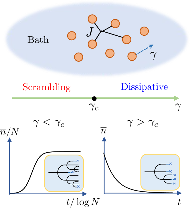
Figure 1: Schematics of the operator size growth in open quantum systems. Here $J$ represents the interaction between system Majorana fermion modes and $\gamma$ represents the hopping between the system and the bath. We find different dynamical phases exist when tunning $\gamma$. For small $\gamma$, the system is in a scrambling phase where the average operator size $\overline{n}$ grows to $O(N)$ values at time $\sim\log N$. For large $\gamma$, the average operator size decays to zero with $O(1)$ rate. Insets are diagrammatic illustrations of the typical operator size growth history in different phases.

In this work, based on semi-classical epidemiological models, we propose the existence of a dynamical transition in open quantum systems with all-to-all interactions at finite system-bath coupling $\gamma$, above which the scrambling process halts; the transition separates a scrambling phase at small $\gamma$ and a dissipative phase at large $\gamma$. We further demonstrate the transition by solving analytically a Brownian SYK model accompanied with a bath Kitaev (2015); Maldacena and Stanford (2016); Kitaev and Suh (2018); Saad et al. (2018); Sünderhauf et al. (2019). We derive the analytic expressions of the operator size distribution both in the early-time and the late-time regimes. The analytic results indicate a two-stage scenario for the operator size growth: in the early stage, the bath operators act as an attractor and continuously absorb the weight from the system operators. If the intrinsic scrambling rate of the open system is not fast enough, all the weight eventually falls into the bath. Only if the system intrinsic scrambling rate is sufficiently large, a finite weight escapes the absorption and survives in the system, and the growth enters into the second stage where, though dragged by the bath, the scrambling process persists and the growth converges to a reduced operator size of the same order as in the closed system. We argue that the scenario shall be generic to a wide class of Brownian SYK models in the presence of baths. We also discuss the implications of our results on the teleportation transition and point out possible relations between our “bath-induced scrambling transition” to the measurement-induced entanglement phase transitions Li et al. (2018); Skinner et al. (2019); Chan et al. (2019).

Operator Size in Open Systems.– Our goal is to study the operator size growth in open quantum systems with all-to-all interactions. We consider a class of chaotic quantum many-body systems $S$ coupled to an external bath $B$; the system $S$ and the bath $B$ consist of $N$ Majorana fermions $\chi_{j}$ ($j=1,2,...,N$) and $M$ Majorana fermions $\psi_{a}$ ($a=1,2,...,M$) respectively. We choose the normalization to be $\chi_{j}^{2}=\psi_{a}^{2}=1$. The total Hamiltonian is given by $H_{\text{tot.}}=H_{S}[\chi]+H_{B}[\psi]+H_{SB}[\chi,\psi]$. We take $M\gg N$ throughout our study such that once information spreads from the system $S$ into the bath $B$, it will not flow back to the system $S$ Chen et al. (2017); Zhang (2019); Almheiri et al. (2019).

We define the operator size distribution in the open quantum systems in the following way. The time evolution of a certain operator $O$ is determined by the Heisenberg equation as $O(t)=e^{iH_{\text{tot.}}t}Oe^{-iH_{\text{tot.}}t}$. We expand the operator $O(t)$ in terms of the complete orthonormal operator basis $\{\chi_{1}^{p_{1}}...\chi_{N}^{p_{N}}\psi_{1}^{q_{1}}...\psi_{M}^{q_{M}}\}$ with $p_{j}$, $q_{a}\in\{0,1\}$:

$$O(t)=\sum_{\{p_{j}\}}\sum_{\{q_{a}\}}c_{\{p_{j}\},\{q_{a}\}}(t)\chi_{1}^{p_{1}}...\chi_{N}^{p_{N}}\psi_{1}^{q_{1}}...\psi_{M}^{q_{M}}.$$ (1)

Due to the system-bath coupling, $O(t)$ generally involves degrees of freedom both of the system $S$ and the bath $B$. In previous studies of closed systems consisting of Majorana fermions $\chi_{j}$, the operator size of a string operator $\chi_{i_{1}}\chi_{i_{2}}...\chi_{i_{n}}$ is defined to be $n$, equal to the number of the Majorana operators Roberts et al. (2018); Qi and Streicher (2019); Zhang and Gu . To generalize to our open quantum systems, we define the size $n$ of the basis operator $\chi_{1}^{p_{1}}...\chi_{N}^{p_{N}}\psi_{1}^{q_{1}}...\psi_{M}^{q_{M}}$ by counting the number of the system Majorana operators $\chi_{j}$, regardless of the bath operators $\psi_{a}$. The operator size distribution $P(n,t)$ for $O(t)$ sums the weight of size $n$ basis operators in the expansion of $O(t)$:

$$P(n,t)=\sum_{\{p_{j}\}}\delta_{n,\sum p_{j}}\sum_{\{q_{a}\}}\left|c_{\{p_{j}\},\{q_{a}\}}(t)\right|^{2}.$$ (2)

We normalize operators $O(t)$ in the way that $\text{Tr}\,O^{\dagger}O=2^{(M+N)/2}$; resultantly $\sum_{n}P(n,t)=1$. The moments of the operator size are given by $\overline{n^{k}}=\sum_{n}n^{k}P(n,t)$.

Epidemiological models have been applied to interpret the results of operator size growth in closed systems with all-to-all interactions Roberts et al. (2018); Qi and Streicher (2019), where the number of elementary Majorana operators $\chi_{j}$ is an analog of the number of patients. For a Hamiltonian $H_{S}$ with $q$-body interactions of strength $J$, the commutator $i[H_{S},O]$ in the Heisenberg equation of $O(t)$ brings about the infection of $(q-2)$ previously unexposed people at a rate $\sim J$. In the early-time regime, the argument based on the epidemiological model leads to the average operator size $\overline{n}$ satisfying $d\overline{n}/dt=J(q-2)\overline{n}\equiv\varkappa\overline{n}$, which reproduces the result obtained by diagrammatic calculations Roberts et al. (2018); Qi and Streicher (2019). Here we have introduced the intrinsic quantum Lyapunov exponent $\varkappa$.

We generalize the argument based on the epidemiological model to the cases of our open systems; we include the system-bath coupling of the form $H_{SB}=i\sum_{ia}\gamma_{ia}\chi_{i}\psi_{a}$, which is due to direct hopping between the system $S$ and the bath $B$. Two additional commutators show up in the Heisenberg equation of $O(t)$: $i[H_{B},O]$ does not change the operator size while $i[H_{SB},O]$ can replace one of the system Majorana operators $\chi_{i}$ by a bath Majorana operator $\psi_{a}$ , and results in decreasing the operator size by one at rate $\gamma$. Conrrespondingly, the epidemiological model shall be modified to give

$$\frac{d\overline{n}}{dt}=\varkappa\overline{n}-\gamma\overline{n}$$ (3)

in the early-time regime. The solution $\overline{n}\sim e^{(\varkappa-\gamma)t}$ indicates two distinct dynamical phases separated by the critical point at $\gamma_{c}=\varkappa$. For $\gamma<\gamma_{c}$, the average operator size increases exponentially in the early-time regime as its counterparts in the closed systems; we take the exponential increase as the defining feature of the scrambling phase, which has been numerically studied in Schuster and Yao (2022). The exponential growth of $\overline{n}$ is expected to terminate at an enhanced scrambling time $t_{s}\sim(\gamma_{c}-\gamma)^{-1}\log N$, where additional information is required to analyze the full operator dynamics. For $\gamma>\gamma_{c}$, the average operator size decreases to exponentially small value after time $(\gamma-\gamma_{c})^{-1}$, which suggests only bath operators remain in the expansion (1); we call this the dissipative phase. At the critical point $\gamma_{c}=\varkappa$, $\overline{n}$ is expected not to change with time. However, as we show below through an explicit model calculation, the operator size distribution $P(n,t)$ is found to exhibit a non-trivial power-law decrease in time $t$ for any $n\geq 1$. Schematics for the operator size growth in different phases are presented in FIG. (1).

Solvable SYK Model.– In the following parts, we demonstrate the existence of the dynamical transition and reveal the dynamics of the operator size distribution in different phases via solvable Brownian SYK models Saad et al. (2018); Sünderhauf et al. (2019), which are closely related to Brownian circuits in spin models Zhou and Chen (2019). The specific class of the Hamiltonians we consider have the form

$$H(t)=\sum_{i_{1}<...<i_{q}}i^{\frac{q}{2}}J_{\{i_{p}\}}(t)\chi_{i_{1}}\chi_{i_{2}}...\chi_{i_{q}}+\sum_{j,a}iV_{ja}(t)\chi_{j}\psi_{a}$$ (4)

for even $q$, and

$$H(t)=\sum_{i_{1}<...<i_{q},a}i^{\frac{q-1}{2}}J_{\{i_{p}\},a}(t)\chi_{i_{1}}\chi_{i_{2}}...\chi_{i_{q}}\psi_{a}+\sum_{j,a}iV_{ja}(t)\chi_{j}\psi_{a}$$ (5)

for odd $q$. We focus on the cases of $q\geq 3$, in which the first term in both (4) and (5) leads to a growth of the operator size $n$. The coupling constants $J_{\{i_{p}\}}(t)$, $J_{\{i_{p}\},a}(t)$, and $V_{ja}(t)$ with different indices are independent Brownian variables and have the property

$$\overline{J_{\{i_{p}\}}(t_{1})J_{\{i_{p}\}}(t_{2})}={(q-1)!J}\delta(t_{1}-t_{2})/{N^{q-1}},$$ (6)

$$\overline{J_{\{i_{p}\},a}(t_{1})J_{\{i_{p}\},a}(t_{2})}={(q-1)!J}\delta(t_{1}-t_{2})/{N^{q-1}M},$$

$$\overline{V_{ja}(t_{1})V_{ja}(t_{2})}={V}\delta(t_{1}-t_{2})/{M}.$$

In the following, we take the limit of $M\gg N\gg 1$ in which our Brownian SYK models can be worked out using the $1/N$ expansion Maldacena and Stanford (2016).

To study the operator size growth, we generalize a method introduced in Qi and Streicher (2019): We construct auxiliary Majorana fermions $\tilde{\chi}_{j}$ and $\tilde{\psi}_{a}$, which are paired up with $\chi_{j}$ and $\psi_{a}$ to form the complex fermions $c_{j}=(\chi_{j}+i\tilde{\chi}_{j})/2$ and $c_{a}^{B}=(\psi_{a}+i\tilde{\psi}_{a})/2$ respectively. We introduce a normalized EPR state $|\text{EPR}\rangle$ which satisfies $c_{j}|\text{EPR}\rangle=c_{a}^{B}|\text{EPR}\rangle=0$; in other words, $|\text{EPR}\rangle$ is the vacuum state of the complex fermion modes. Consequently, when we apply $O(t)$ to $|\text{EPR}\rangle$, the complex fermion number can never decrease. In particular, for a string operator of the Majorana fermions, each Majorana operator $\chi_{j}/\psi_{a}$, when acting on $|\text{EPR}\rangle$, creates one excitation $c^{\dagger}_{j}/c^{B,\dagger}_{a}$. Thus the operator size distribution can be calculated via $P(n,t)=\langle O(t)^{\dagger}\Pi(n)O(t)\rangle$, where $\Pi(n)$ is the projection operator into the subspace with $n$ excitations of $c^{\dagger}_{j}$ while leaving the number of $c^{B,\dagger}_{a}$ excitations arbitrary. The expectation values $\langle\dots\rangle$ are taken with respect to $|\text{EPR}\rangle$.

It is more convenient to work with the generating function $z(\mu,t)=\sum e^{-\mu n}P(n,t)$, which takes the form

$$z(\mu,t)=\langle O(t)^{\dagger}e^{-\mu\sum_{j}c^{\dagger}_{j}c_{j}}O(t)\rangle.$$ (7)

In particular, the average operator size is equal to the summation of out-of-time-order commutators between $O$ and $\chi_{j}$:

$$\overline{n}=-\partial_{\mu}z(0,t)=\frac{1}{4}\sum_{j}\left\langle\left|[O(t),\chi_{j}]\right|^{2}\right\rangle,$$ (8)

where the commutator shall be replaced by the anti-commutator if $O$ is fermionic.

In the following discussions, we focus on the case $O=\chi_{1}$, which is the simplest non-trivial operator. The retarded Green’s functions $G^{R}(t)\equiv-i\theta(t)\left<\{\chi_{i}(t),\chi_{i}(0)\}\right>$ can be worked out by using the path-integral approach on the Keldysh contour as in Zhang et al. (2020); we find:

$$G^{R}(\omega)^{-1}=\omega/2-\Sigma^{R},\ \ \ \ \ \Sigma^{R}=-i(J+V)\equiv-i\Gamma/4,$$ (9)

where the quasi-particle decay rate $\Gamma$ is independent of $q$. After the Fourier transform, we have $G^{R}(t)=-2i\theta(t)e^{-\Gamma t/2}$. The generating function (7) turns into a two-point function on the double Keldysh contour Aleiner et al. (2016) with a perturbation source:

$$\Delta I=\frac{1}{4}(1-e^{-\mu})\sum_{j}\left[\chi_{j}^{u_{2}}(0)-\chi_{j}^{d_{2}}(0)\right]\left[\chi_{j}^{d_{1}}(0)-\chi_{j}^{u_{1}}(0)\right].$$ (10)

Here $\chi_{j}^{u_{k}/d_{k}}(t)$ labels the Majorana fields on the double Keldysh contour Zhang et al. (2020): $u/d$ denotes the forward/backward evolution and $k=1$ or $2$ labels the two worlds. The factor $(1-e^{-\mu})$ appears because for coherent states $|\psi\rangle$, $\langle\bar{\psi}|e^{-\mu c^{\dagger}c}|\psi\rangle=e^{-e^{-\mu}\bar{\psi}\psi}$.

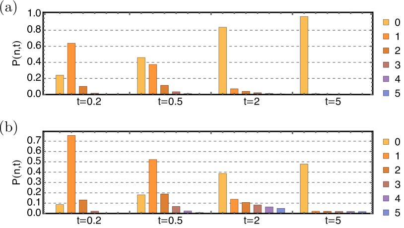
Figure 2: The plot for the early-time operator size distribution $P(n,t)$ with $q=3$ and $J=1/4$ in different phases: (a) In the dissipative phase with $r=V/J=3/2$, the operator weight for $n\geq 1$ decays to zero quickly. (b) In the scrambling phase with $r=V/J=1/2$, the operator weight at $n=0$ saturates to $P(0,t)=r$, leaving finite weight on operators with $n\geq 1$.

Early-time Operator Dynamics.– In the early-time regime with $t\ll t_{s}$, we can derive the two-point function $z(\mu,t)$ using the saddle-point equation and have SM

$$z(\mu,t)=-\int dt^{\prime}~{}G^{R}(t-t^{\prime})^{2}\Sigma_{W}(t^{\prime}),$$ (11)

$$\Sigma_{W}(t)=Jz(\mu,t)^{q-1}+V-\frac{1}{4}(1-e^{-\mu})\delta(t).$$

For $t<0$, the system is in equilibrium and $z=1$. At $t=0$, the last term in $\Sigma_{W}$ leads to an instant change of $z$. By applying $(\partial_{t}+\Gamma)$ to both sides of the first line of (11), we find

$$\frac{dz}{dt}=4J(z^{q-1}-z)+4V(1-z),\ \ \ \ \ z(\mu,0^{+})=e^{-\mu}.$$ (12)

which determines the early-time operator size growth in the open quantum system.

We analyze (12) by firstly examining the early-time evolution of $\overline{n}$. Taking derivative with respective to $\mu$ and set $\mu=0$, we have

$$\frac{d\overline{n}}{dt}=4J(q-2)\overline{n}-4V\overline{n},$$ (13)

which matches (3) with identifications $\varkappa=4J(q-2)$ and $\gamma=4V$. This agreement suggests that the solvable SYK models we constructed show the dynamical phase transition between the scrambling phase and the dissipative phase.

To fully characterize the operator dynamics in the early-time regime, we need to solve the generating function via (12). In the following discussions, we would focus on $q=3$ where the evolution of the operator size distribution can be computed in closed-form.

From now on, we set $J=1/4$ and introduce $r\equiv V/J$ for conciseness. Assuming $r\neq 1$, by integrating the differential e quation (12) for $q=3$, the solution reads

$$z(\mu,t)=1-\frac{(r-1)(1-e^{-\mu})}{e^{(r-1)t}(r-e^{-\mu})-(1-e^{-\mu})}.$$ (14)

Expanding in terms of $e^{-\mu}$, we find the operator size distribution at early time $t\ll t_{s}$:

$$P(n,t)=\begin{cases}1-(1-r)\frac{e^{(1-r)t}}{e^{(1-r)t}-r},&(n=0)\\ (1-r)^{2}\frac{e^{(1-r)t}[e^{(1-r)t}-1]^{n-1}}{[e^{(1-r)t}-r]^{n+1}}.&(n\geq 1)\end{cases}$$ (15)

In the dissipative phase with $r>1$, $z(\mu,t)$ increases from $e^{-\mu}$ towards unity as time increases for any $\mu>0$, which indicates that $\chi_{1}(t)$ only contains the bath operators in the long term. This trend is because $z=1$ is the stable fixed point in (12). Correspondingly, (15) shows the operator weight is localized near $n=0$, with an exponentially decaying tail $P(n,t)\sim e^{-n/\xi(t)}$ and $\xi(t)=1/\ln[(r-e^{(1-r)t})/(1-e^{(1-r)t})]$. This feature is illustrated in FIG. 2 (a) for $r=3/2$.

On the other hand, in the scrambling phase $r<1$, $z(\mu,t)$ changes from $e^{-\mu}$ to a non-zero value $r$ since the fixed point $z=1$ is now unstable. It is known that in closed systems, the out-of-time-order correlation decays to zero after a perturbation Aleiner et al. (2016). In our open quantum systems, a finite residual correlation instead survives due to the coupling induced by the bath $B$, which is reflected by the saturation $P(0,t)\approx r$ for $(1-r)t\gg 1$; since the distribution is normalized, the sum of the operator weight at $n\geq 1$ is always finite. Furthermore, (15) shows that the operators with size $1\leq n\lesssim e^{(1-r)t}$ are occupied by the same order, as illustrated in FIG. 2 (b). Outside the early-time regime, when $t\gtrsim t_{s}$, a typical operator would have size $\sim N$ in the scrambling phase, and the saddle-point description (11) is no longer sufficient Gu et al. (2022). It is necessary to go beyond and employ the full scramblon effective theory Gu et al. (2022); Zhang and Gu to compute the operator size distribution .

Before turning to the late-time regime, we comment on the critical phase with $r=1$. Instead of (14) and (15), we have

$$z(\mu,t) =1-\frac{1-e^{-\mu}}{1+t(1-e^{-\mu})},$$ (16)

$$P(n,t) =\begin{cases}1-\frac{1}{1+t},&(n=0)\\ \frac{t^{n-1}}{(1+t)^{n+1}}.&(n\geq 1)\end{cases}$$

As in the scrambling phase, the occupied operators extend to large $n$: the operators with $1\leq n\lesssim t$ are occupied by the same order. However, for $t\gg 1$, $z(\mu,t)\to 1$; all the information dives into the bath $B$. Consequently, there are no non-trivial dynamics in the late-time regime.

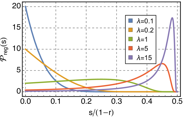
Figure 3: The plot for the late-time operator size distribution $\mathcal{P}_{\text{reg}}(s,t)$ with $q=3$ and $J=1/4$ in the scrambling phase ($r<1$) for different $\lambda=e^{(1-r)t}/C$ with $C=N(1-r)^{2}/2$. When $\lambda$ is fixed, $\mathcal{P}_{\text{reg}}(s,t)$ for different $r$ collapse to a universal function of $s/(1-r)$.

Scrambling at the Late Time.– We now study the late-time operator size distribution in the scrambling phase using the scramblon effective theory Gu et al. (2022). Since in the late-time regime a typical operator has size $n\propto N$, we consider a continuum limit with $s=n/N\in[0,1]$ and $\mathcal{P}(s,t)\equiv NP(n,t)$ as in the closed quantum systems Zhang and Gu . We have $\int_{0}^{1}ds~{}\mathcal{P}(s,t)=1$, and the generating function

$$\mathcal{S}(\nu,t)\equiv\int_{0}^{1}ds~{}e^{-\nu s}\mathcal{P}(s,t)=z({\nu}/{N},t).$$ (17)

Our task is to compute $\mathcal{S}(\nu,t)$ for $t\sim t_{s}$ by making use of $z(\mu,t)$ obtained for $t\ll t_{s}$.

The crucial observation is that important corrections to the saddle-point solution are only induced by the interaction between fermions that are mediated by scramblon modes, which have a soft action Stanford et al. (2022). The scramblon propagator and the scattering vertices between fermions and scramblons can be determined using (14) for $z(\mu,t)$. The late-time operator-size distribution $\mathcal{S}(\nu,t)$ is then computed by summing up scramblon diagrams to the leading order in $1/N$ as in Zhang and Gu . The final result is given by SM

$$\mathcal{P}(s,t)= r\delta(s)+\mathcal{P}_{\text{reg}}(s,t)$$ (18)

$$\mathcal{P}_{\text{reg}}(s,t)= \theta\left(1-\frac{2s}{1-r}\right)\frac{2(r-1)^{2}e^{\frac{2s}{\lambda(r+2s-1)}}}{\lambda(r+2s-1)^{2}},$$

where $\lambda=e^{(1-r)t}/C$ with $C=N(1-r)^{2}/2$ is the propagator of the scramblons. The singular part $\delta(s)$ is consistent with the saturation value of $P(0,\infty)$ derived in (15). This part means that in the late-time regime, the weight of pure bath operators does not change. This is because the typical operators appearing in the expansion contain $O(N)$ system fermions, which have negligible coupling to the $n=0$ operators. The regular part $\mathcal{P}_{\text{reg}}(s,t)$ describes operators scrambled into the large size, with a total weight $(1-r)$. Interestingly, it is only a function of $s/(1-r)$. For closed quantum systems, the operator becomes maximally scrambled in the long-time limit ($t\rightarrow\infty$), which corresponds to a delta peak at $s=1/2$ Zhang and Gu . However, in our open systems, we see that the effect of the system-bath coupling is to exert a “drag force” and renders the analog of the maximally scrambled operator having a typical size $s=(1-r)/2$. A plot of $\mathcal{P}_{\text{reg}}(s,t)$ is presented in FIG. 3. Using (18), we could also compute moments of the operator size $\overline{n^{k}}$. As an example, we find the average operator size reads

$$\overline{n}=N\overline{s}=N\frac{(1-r)^{2}}{2}{\left[1-\frac{1}{\lambda}e^{\frac{1}{\lambda}}\Gamma\left(0,\frac{1}{\lambda}\right)\right]},$$ (19)

which increases monotonically to the saturation value $N\frac{(1-r)^{2}}{2}$.

Discussions.– In this work, based on the epidemiological models and the solvable Brownian SYK models, we show that couplings to external baths can give rise to a dynamical transition of the operator size growth in open quantum systems. The explicit analytic results obtained for the solvable Brownian SYK model of $q=3$ suggest that the operator growth consists of two stages: in the first stage, the bath operators keep absorbing weight from the system operators. If the intrinsic scrambling of the system is strong enough, a finite weight would manage to escape the absorption, and in the second stage, the operator size distribution $\mathcal{P}(s,t)$ has the same scaling form as when the system is closed. Since (12) is the base for our analysis of the case of $q=3$, we expect that the existence of the dynamic transition stand as well for $q>3$ from (12) SM .

The dynamic transition separating the dissipative and scrambling phases implies that teleportation through the wormhole Gao et al. (2017); Maldacena et al. (2017); Susskind and Zhao (2018); Gao and Liu (2019); Brown et al. (2019); Gao and Jafferis (2021); Nezami et al. (2021); Gu et al. is still possible when an environment is added if the scrambling of the initial operator into the holographic bulk is fast enough. However, the amount of information that can be teleported is reduced. Our “bath-induced scrambling phase transition” shall have a close relation with the celebrated “measurement-induced entanglement phase transition” Li et al. (2018); Skinner et al. (2019); Chan et al. (2019). In particular, after integrating out the bath which is assumed to be Markovian, the evolution of the operator size (7) can be formulated in terms of a generalized master equation, which was introduced to study the measurement-induced entanglement phase transition Zhou (2022). The volume-law phase in the presence of measurement is known to be protected from local quantum errors Gullans and Huse (2020); Choi et al. (2020); Fan et al. (2021), so is expected the scrambling phase in open systems. Furthermore, the averaged operator size (8) conveys information similar as the entropy of a system Hosur et al. (2016); Fan et al. (2017). We postpone a detailed study to future works.

Acknowledgment. We thank Chang Liu for helpful discussions. PZ is partly supported by the Walter Burke Institute for Theoretical Physics at Caltech. ZY is supported by the National Natural Science Foundation of China (Grant No. 12074440), and Guangdong Project (Grant No. 2017GC010613).

Note Added. When completing this work, we noted that a scrambling transition was also revealed in a random unitary circuit that exchanges qubits with an environment Weinstein et al. (2022). The study focused on the numerical evidence from the out-of-time-order correlator.

In this Supplementary Material, we present the derivations of (1) the self-consistent equation for the generating function $z(\mu,t)$; (2) the late-time operator size distribution $\mathcal{P}(s,t)$; (3) the analysis of the operator size dynamics for $q\geq 4$.

I the self-consistent equation for the generating function

In this section, we present the derivation of

$$z(\mu,t)=-\int dt^{\prime}~{}G^{R}(t-t^{\prime})^{2}\Sigma_{W}(t^{\prime}),\ \ \ \ \ \ \Sigma_{W}(t)=Jz(\mu,t)^{q-1}+V-\frac{1}{4}(1-e^{-\mu})\delta(t),$$ (20)

for the generating function $z(\mu,t)=\sum e^{-\mu n}P(n,t)$ as stated in the main text. The idea is to write out the path-integral representation of Gu et al. (2022).

$$z(\mu,t)=\langle\text{EPR}|\chi_{1}(t)^{\dagger}e^{-\mu\sum_{j}c^{\dagger}_{j}c_{j}}\chi_{1}(t)|\text{EPR}\rangle,$$ (21)

where $z(\mu,t)$ is a two-point function with a perturbation source, and derive (20) by using the Schwinger-Dyson equation.

As a warm-up, we first consider the average operator size, which is the first moment of $z(\mu,t)$:

$$\overline{n}=\sum_{j}\langle\text{EPR}|\chi_{1}(t)^{\dagger}c^{\dagger}_{j}c_{j}\chi_{1}(t)|\text{EPR}\rangle=\frac{1}{4}\sum_{j}\left(\langle\chi_{1}(t)\chi_{j}\chi_{1}(t)\chi_{j}\rangle+\langle\chi_{j}\chi_{1}(t)\chi_{1}(t)\chi_{j}\rangle+\langle\chi_{j}\chi_{1}(t)\chi_{j}\chi_{1}(t)\rangle+\langle\chi_{1}(t)\chi_{j}\chi_{j}\chi_{1}(t)\rangle\right).$$ (22)

The calculation of $\overline{n}$ can be represented as a four-point function on the double Keldysh contour Aleiner et al. (2016)

(23)

which contains two forward evolution branches $(u_{1},u_{2})$ and two backward evolution branches $(d_{1},d_{2})$. The black points represent the insertions of $\chi_{1}$ and the red points represent the insertions of $\chi_{j}$. More explicitly, we have

$$\overline{n}=\frac{1}{4}\sum_{j}\left<T_{\mathcal{C}}\,\chi^{u_{2}}_{1}(t)\chi^{u_{1}}_{1}(t)\left[\chi_{j}^{u_{2}}(0)-\chi_{j}^{d_{2}}(0)\right]\left[\chi_{j}^{d_{1}}(0)-\chi_{j}^{u_{1}}(0)\right]\right>.$$ (24)

Here the minus sign is from the anti-commutation relation of Grassmann fields, and $T_{\mathcal{C}}$ is the contour ordering operator. Generalizing the derivation to $z(\mu,t)$, we find

$$z(\mu,t) =\left<T_{\mathcal{C}}\,\chi^{u_{2}}_{1}(t)\chi^{u_{1}}_{1}(t)e^{-\Delta I}\right>,\ \ \ \ \ \ \Delta I=\frac{1}{4}(1-e^{-\mu})\sum_{j}\left[\chi_{j}^{u_{2}}(0)-\chi_{j}^{d_{2}}(0)\right]\left[\chi_{j}^{d_{1}}(0)-\chi_{j}^{u_{1}}(0)\right].$$ (25)

Here $(1-e^{-\mu})$ appears instead of $\mu$ since we have $\langle\bar{\psi}|e^{-\mu c^{\dagger}c}|\psi\rangle=e^{-e^{-\mu}\bar{\psi}\psi}$. The two-point function $z(\mu,t)$ is the equal time limit of the inter-world Wightmann function $G_{W}(t_{1},t_{2})=\left<\chi^{u_{2}}(t_{1})\chi^{u_{1}}(t_{2})\right>_{\Delta I}$, which satisfies the Schwinger-Dyson equation Gu et al. (2022)

$$G_{W}(t_{1},t_{2})=\int dt_{3}dt_{4}~{}G_{R}(t_{1},t_{3})\Sigma_{W}(t_{3},t_{4})G_{A}(t_{4},t_{2}).$$ (26)

For our Brownian SYK models, the self-energy takes a simple form:

$$\Sigma_{W}(t,t^{\prime})=\delta(t-t^{\prime})\left(JG_{W}(t,t)^{q-1}+V-\frac{1}{4}(1-e^{-\mu})\delta(t)\right)\equiv\delta(t-t^{\prime})\Sigma_{W}(t).$$ (27)

Using (26), $\eqref{supp:SD2}$, and $G_{R}(t_{1},t_{2})=-G_{A}(t_{2},t_{1})$, we arrive at (20) after taking $t_{1}=t_{2}=t$.

II the late-time operator size distribution

Here we derive the late-time operator size distribution in the scrambling phase $r<1$:

$$\mathcal{P}(s,t)=r\delta(s)+\mathcal{P}_{\text{reg}}(s,t)=r\delta(s)+\theta\left(1-\frac{2s}{1-r}\right)\frac{2(r-1)^{2}e^{\frac{2s}{\lambda(r+2s-1)}}}{\lambda(r+2s-1)^{2}}.$$ (28)

In the long-time limit $e^{(1-r)t}\gg 1$, we assume the perturbation source $\Delta I$ interacts with $\chi_{1}(t)$ only by the exchanging collective scramblon mode. The scramblon mode is the origin of quantum many-body chaos, which has an exponential propagator $-e^{(1-r)t}/C$ with $C\propto N$ Gu and Kitaev (2019); Gu et al. (2022). We define the scattering between the fermion fields and the scramblons as

$$\leavevmode\hbox to34.78pt{\vbox to29.29pt{\text{[drawing]}}}=\Upsilon^{R,m},\ \ \ \ \ \ \leavevmode\hbox to41.45pt{\vbox to29.29pt{\text{[drawing]}}}=\Upsilon^{A,m}.$$ (29)

Here for simplicity, we assumed all the fermion fields are inserted (in the future for $\Upsilon^{R}$ and in the past for $\Upsilon^{A}$ ) at the same time. In particular, since our models have time-reversal symmetry, we have $\Upsilon^{R,m}=\Upsilon^{A,m}=\Upsilon^{m}$.

To determine $\Upsilon^{R/A,m}$, we turn to the early-time form of the generating function

$$z(\mu,t)=1-\frac{(r-1)(1-e^{-\mu})}{e^{(r-1)t}(r-e^{-\mu})-(1-e^{-\mu})}.$$ (30)

We consider the situation $\mu\ll 1$ and $1\ll e^{(1-r)t}\lesssim 1/\mu\ll N$, under which all non-scramblon contribution vanishes; we find

$$z(\mu,t)=r+\frac{1-r}{1+e^{(1-r)t}\mu(1-r)^{-1}}.$$ (31)

On the other hand, the scramblon contribution to the early-time generating function takes the form:

$$z(\mu,t)=\leavevmode\hbox to69.35pt{\vbox to69.09pt{\text{[drawing]}}}=\sum_{m=0}^{\infty}\left(-\frac{e^{(1-r)t}}{C}\right)^{m}\left(\frac{\mu N}{2}\Upsilon^{1}\right)^{m}\frac{\Upsilon^{m}}{m!}. 3 4 3 4$$ (32)

Here each insertion of $\Delta I$ only creates a single scramblon due to the suppression $\lambda\sim O(1/N)$. In fact, we have not fixed the normalization of the scramblon field. The transformation $C\rightarrow a^{2}C$ and $\Upsilon^{m}\rightarrow a^{m}\Upsilon^{m}$ leaves the expression invariant. We could make a convenient choice

$$\frac{N\Upsilon^{1}}{2C}=(1-r)^{-1},$$ (33)

and define

$$f(x)=\sum_{m=0}^{\infty}\frac{(-x)^{m}}{m!}\Upsilon^{m}=r+\frac{1-r}{1+x}.$$ (34)

By expanding $f(x)$, we can fix $\Upsilon^{m}$. In particular, we find

$$\Upsilon^{0}=1,\;\;\;\;\;\Upsilon^{m}=(1-r)\,m!,\;\;\;\;\;C=N(1-r)^{2}/2.$$ (35)

Now we consider the late-time operator size generating function $\mathcal{S}(\nu,t)$ with $\lambda\sim O(1)$. Unlike the early-time result, we need to sum up all diagrams where each insertion of $\Delta I$ create arbitrary number of scramblons:

$$\mathcal{S}(\nu,t)=\leavevmode\hbox to69.35pt{\vbox to69.09pt{\text{[drawing]}}}=e^{-\frac{\nu}{2}}\sum_{n=0}^{\infty}\frac{(\nu/2)^{n}}{n!}\sum_{\{m_{j}\geq 0\}}(-\lambda)^{\sum_{j}m_{j}}\frac{\Upsilon^{\sum_{j}m_{j}}\Upsilon^{m_{1}}\ldots\Upsilon^{m_{n}}}{m_{1}!m_{2}!\ldots m_{n}!} 3 4 3 4$$ (36)

We introduce $h(y)$ as the inverse Laplace transform of $f(x)$:

$$f(x)=\int_{0}^{\infty}dy~{}e^{-xy}h(y),\ \ \ \ \ \ h(y)=(1-r)e^{-y}+r\delta(y).$$ (37)

By comparing with (34), we find

$$\Upsilon^{m}=\int_{0}^{\infty}dy~{}y^{m}h(y).$$ (38)

This leads to

$$\mathcal{S}(\nu,t) =\int_{0}^{\infty}dy~{}h(y)~{}e^{-\frac{\nu}{2}}\sum_{n=0}^{\infty}\frac{(\nu/2)^{n}}{n!}\sum_{\{m_{j}\geq 0\}}(-\lambda)^{\sum_{j}m_{j}}\frac{y^{\sum_{j}m_{j}}\Upsilon^{m_{1}}\ldots\Upsilon^{m_{n}}}{m_{1}!m_{2}!\ldots m_{n}!}$$ (39)

$$=\int_{0}^{\infty}dy~{}h(y)~{}e^{-\frac{\nu}{2}}\sum_{n=0}^{\infty}\frac{(\nu/2)^{n}}{n!}\left[\sum_{\{m\geq 0\}}(-\lambda)^{m}\frac{y^{m}\Upsilon^{m}}{m!}\right]^{n}$$

$$=\int_{0}^{\infty}dy~{}h(y)~{}e^{-\frac{\nu}{2}}\sum_{n=0}^{\infty}\frac{(\nu/2)^{n}}{n!}f(\lambda y)^{n}$$

$$=\int_{0}^{\infty}dy~{}h(y)e^{-\frac{\nu}{2}\left(1-f(\lambda y)\right)},$$

Performing the inverse inverse Laplace transform with respect to $\nu$, we find

$$\mathcal{P}(s,t) =\int_{0}^{\infty}dy~{}h(y)\delta\left(s-\frac{1-f(\lambda y)}{2}\right).$$ (40)

Integrating over $y$ in (40) leads to the result (28).

III dynamical trnsition of the opertaor size for general ${q}\geq 3$

In the main text, we first use the epidemiological models to predict the existence of the bath-induced scrambling transition. Later, we work out explicitly the operator size distribution for the Brownian SYK model of $q=3$; using the early-time generating function, we find $P(0,\infty)=1$ in the dissipative phase and $P(0,\infty)<1$ in the scrambling phase. In the following, we show that certain features of the transition are independent of $q$ for the Brownian SYK model of general $q\geq 3$, i.e.,

1. For $r<q-2$, we have $P(0,\infty)<1$. Together with the exponential growth of the operator size $\overline{n}$ in the early-time regime, this indicates the intrinsic scrambling of the system is strong enough, a finite weight would manage to escape the absorption.

2. For $r\geq q-2$, we have $P(0,\infty)=1$. Since we have the normalization $\sum_{n}P(n,t)=1$, this indicates the system is in the dissipative phase where a typical operator at late time contains no system operator.

We start with the differential equation satisfied by the early-time generating function

$$\frac{dz}{dt}=(z^{q-1}-z)+r(1-z),\ \ \ \ \ z(\mu,0^{+})=e^{-\mu}.$$ (41)

Integrating (41) directly, we find

$$t=\int_{e^{-\mu}}^{z(\mu,t)}d\tilde{z}\frac{1}{(\tilde{z}^{q-1}-\tilde{z})+r(1-\tilde{z})}.$$ (42)

By definition, we have $P(0,t)=z(\infty,t)$. This relation gives rise to

$$t=\int_{0}^{P(0,t)}d\tilde{z}\frac{1}{(\tilde{z}^{q-1}-\tilde{z})+r(1-\tilde{z})}.$$ (43)

For $t\rightarrow\infty$, the L.H.S. of (43) diverges. As a result, $P(0,\infty)$ should coincide with the pole of the integrand, namely,

$$P(0,\infty)^{q-1}-(r+1)P(0,\infty)+r=0.$$ (44)

Moreover, since $P(0,t=0)=0$, $P(0,\infty)$ should be the smallest real positive root of $u(x)=x^{q-1}-(r+1)x+r$. It is straightforward to check that $x_{r}=1$ is always a root of $u(x)$. For $q\geq 3$, $u^{\prime\prime}(x)>0$ for $x>0$. Considering the fact that $u(0)=r>0$ and $u(1)=0$, we have one additional root $x_{r}^{\prime}<1$ if and only if

$$u^{\prime}(1)=(q-2-r)>0.$$ (45)

This is satisfied when $r<q-2$. As a result, we have $P(0,\infty)<1$ for $r<q-2$ and $P(0,\infty)=1$ for $r\geq q-2$, as stated at the beginning of the section.