Validation tests of GBS quantum computers give evidence for quantum advantage with a decoherent target

Abstract

Computational validation is vital for all large-scale quantum computers. One needs computers that are both fast and accurate. Here we apply precise, scalable, high order statistical tests to data from large Gaussian boson sampling (GBS) quantum computers that claim quantum computational advantage. These tests can be used to validate the output results for such technologies. Our method allows investigation of accuracy as well as quantum advantage. Such issues have not been investigated in detail before. Our highly scalable technique is also applicable to other applications of linear bosonic networks. We utilize positive-P phase-space simulations of grouped count probabilities (GCP) as a fingerprint for verifying multi-mode data. This is exponentially more efficient than other phase-space methods, due to much lower sampling errors. We randomly generate tests from exponentially many high-order, grouped count tests. Each of these can be efficiently measured and simulated, providing a quantum verification method that is non-trivial to replicate classically. We give a detailed comparison of theory with a 144-channel GBS experiment, including grouped correlations up to the largest order measured. We show how one can disprove faked data, and apply this to a classical count algorithm. There are multiple distance measures for evaluating the fidelity and computational complexity of a distribution. We compute these and explain them. The best fit to the data is a partly thermalized Gaussian model, which is neither the ideal case, nor the model that gives classically computable counts. Even with a thermalized model, discrepancies of $Z>100$ were observed from some $\chi^{2}$ tests, indicating likely parameter estimation errors. Total count distributions were much closer to a thermalized quantum model than the classical model, giving evidence consistent with quantum computational advantage for a modified target problem.

I Introduction

Computers of all types require validation. Yet this is nontrivial with quantum computers which claim quantum advantage, since the outputs are not classically computable [1, 2, 3, 4, 5]. There is much recent research on this topic due to decoherence and noise which both limits the quantum advantage obtainable, and can lead to erroneous results [6]. The challenge with any classical or quantum computer is that there are exponentially many possible logical programs to test. Verification of large gate-based quantum computers is currently restricted to sub-classes of programs that allow benchmarking, or else uses extrapolation to larger sizes than can be verified directly [7]. When problems have random number outputs, the distributions are usually exponentially sparse, which in standard practice requires binning the data to measure probabilities in order to do statistical testing [8].

Bosonic networks employed as quantum computers combine all three of these validation challenges of hardness, exponentially many combinations, and output sparseness. They are developing at an increasingly rapid pace due to their high degree of scalability. These networks include boson samplers, which utilize either nonclassical input number states [1, 9, 10, 11, 12, 13, 14, 15] or Gaussian squeezed states [2, 16, 3, 17, 18, 19] to generate random, discrete counts by sampling matrix permanents, Hafnians, or the Torontonian [20, 1, 2, 3]. Which distribution is sampled depends on the input state and detectors used. All of these variants have output counting distributions which are exponentially hard to either compute or sample for photonic networks of large size [21, 22].

In this paper, we expand upon earlier work which showed how one can use grouped count probabilities (GCPs) to validate outputs of Gaussian boson sampling (GBS) quantum computers with threshold detectors [23, 24]. This is achieved with scalable simulations using phase-space mapping to continuous samples. These techniques allow one to compare theoretical and experimental output correlations and marginal probabilities, as the simulations have identical moments and correlations to the ideal GBS outputs. These methods have been scaled to exceptionally large sizes of up to 16,000 modes [23]. Because these methods can include decoherence, they can model practical experiments as well as ideal distributions. Here our quantum predictions are compared with a 144-mode experiment claimed to display quantum advantage. We explain how these techniques can distinguish quantum data from classical fakes, even in the regime where there is decoherence and noise present.

GBS experiments are in the hard domain for more than a hundred modes, and are used for random number generation. There are other, much larger bosonic networks in development. These are designed to solve hard optimization problems with up to 100,000 modes, [25, 26, 27, 28, 29, 30], or even large cluster states with up to a million modes [31]. While such larger systems have more practical applications, the GBS case has great scientific interest because quantum advantage is difficult to prove. It has an architecture that allows a detailed theoretical model. By comparing theory with experiment, one can understand how to validate network-based quantum computers, and how to test for experimental imperfections.

The successive large scale implementations of GBS quantum computers claiming quantum supremacy [17, 18, 19] have lead to an outpacing of previous classical verification methods. These either directly compute samples of output distributions such as the Torontonian, for small mode numbers [32, 33], or compute low-order marginal probabilities at larger mode numbers [34, 35]. Practically, these methods are applied to verify GBS outputs for small numbers of modes, since neither method can verify all moments of experimental networks. This is due to such classical methods encountering severe computational barriers when computing high-order correlations, because the full distribution itself is known to be a #P-hard computational problem.

As network sizes continue to increase, verifying high-order correlations becomes increasingly important. Despite this computational hardness, a testing protocol is essential to ensure that experimental errors such as parameter drift, decoherence and noise are negligible. Our phase-space methods can validate all measurable correlations, because they do not use discrete counts. Doing this would be the #P-hard computational problem implemented by the current generation of GBS devices. The positive-P method overcomes this by generating continuous random outputs with equivalent moments, with similar or better accuracy to experimental measurement. Validating the outputs is a different computational task from generating all discrete random counts.

Validation tests can also be used to show a classical imitation is significantly different from the required output, to eliminate fakes. To do this, our methods can generate exponentially many tests by randomly permuting the output groups or bins. Such tests cannot all be implemented at once.

Any attempt to fake the output counts will encounter a computationally hard “shell-game”. The counterfeiter cannot predict which test will be used. Thus, any classical algorithm designed just to deceive a small number of such tests will fail, in all except an exponentially small number of scenarios. While we cannot rigorously eliminate every fake, we conjecture that these randomized tests are computationally hard to pass using classical means, provided there is enough experimental data.

Such tests were performed using GCPs that are binned in multiple dimensions. Multi-dimensional comparisons allow both a fine tuned comparison of experimental outputs with theory, and an exceptionally powerful method to differentiate between fake classical algorithms and experimental data. Comparisons are made with data from a 144-mode GBS experiment using threshold detectors, with measurements of up to $133$-th order correlations [18]. To demonstrate how grouped photon counts can differentiate between experimental and faked correlations, we compare simulations of the ideal GBS output with faking strategies that generate discrete random photon counts. These are generated from classical squeezed thermal states [36, 37], also called squashed states [38, 39], which are input into the linear network.

Comparisons of marginal click correlation moments are also presented, as our numerical method allows one to efficiently generate comparisons for all possible output mode combinations. These are often used to compare the accuracy of samples from experiments that claim the presence of nontrivial correlations [18], with low-order marginal probability based classical algorithms [34].

An analysis of scaling due to sampling errors generated from increased correlation order is given, as normally-ordered positive-P phase-space representations have no vacuum noise, and are therefore very efficient in simulating photo-detection. Due to its reduced sampling errors, the positive-P method [40] is applicable to existing large-scale data sets, and is exponentially faster than non-normally ordered methods [41].

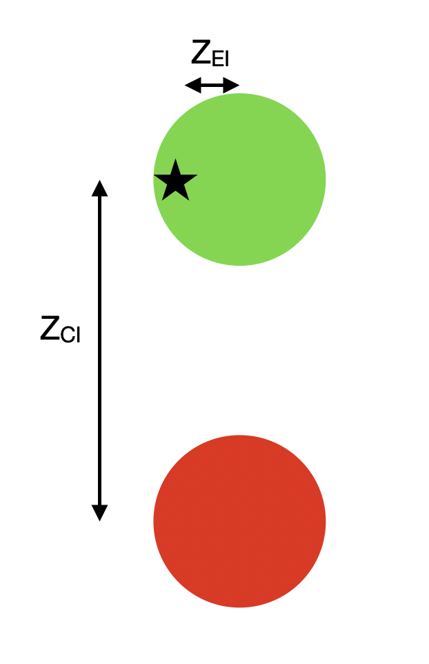
Figure 1: A schematic diagram of the goal of a GBS experiment, in which the star indicates the ideal or target distribution (I), the green circle the sampled distribution from an experiment, and the red circle the nearest efficiently simulable distribution using classical methods. Ideally, one should have $Z_{EI}\lesssim 1$, while $Z_{CI}\gg 1$. This indicates that no classical computer can generate the required distribution, while the quantum computer does. Here $Z$ is a statistical distance measure obtained from $\chi^{2}$ test data, normalized primarily by the experimental sampling errors.

The diagram of Figure (1) shows the goal of the experiment, which is to demonstrate quantum computational advantage. This requires that the experimental data agrees with the ideal theory, $Z_{EI}\lesssim 1$, while no efficient classical simulation can do this, $Z_{CI}\gg 1$. Here $Z$ measures the distribution distance in units of the sampling error. Results of comparisons for all observables using $\chi^{2}$ statistical tests demonstrate that the present 144-mode experimental data set shows large deviations from the ideal GBS distribution, with deviations of over $Z_{EI}\gg 100$ for all data sets, indicating the first requirement is not met. These deviations are highlighted when classically generated binary patterns are compared to the ideal distribution. These show better agreement than experiments with the ideal model.

The comparison of theory to experiment is greatly improved when additional thermalization is included in the squeezed input model. Hence, a more realistic goal is to have $Z_{ET}\lesssim 1$, with $Z_{CT}\gg 1$, which would indicate a computational advantage for the thermalized model. While most of the data does not achieve this, it is obtained for the total count distribution of one of the tested data sets. This situation is indicated in Fig (2).

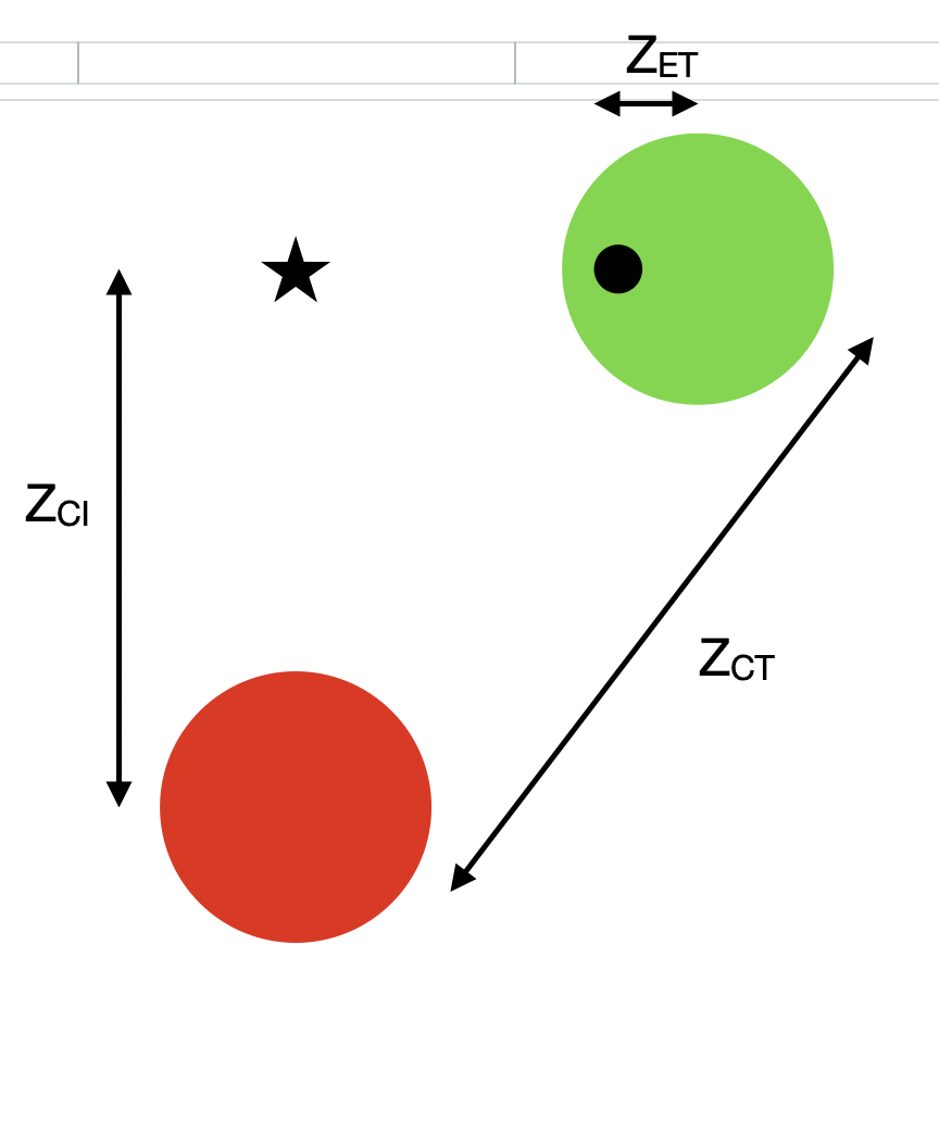
Figure 2: A schematic diagram of the “best-case” of current GBS experiments, with red and green circles as in Fig (1), while the black circle gives the thermalized distribution (T). In this realistic case, one may require that $Z_{ET}\lesssim 1$, while $Z_{CT}\gg 1$. This indicates that no known efficient classical algorithm can generate the thermalized target distribution, while the quantum computer does.

In other cases, while the residual differences are significant, when classical photon counts are compared with this nonclassical but thermalized model, their total count distributions are further from the thermalized distribution than the experiment, shown schematically in Fig (3).

The residual differences may be caused by fluctuations of the network, parameter estimation errors, or nonlinear effects, and are identified by computing the $Z$-statistic. Comparisons of low-order marginals are also performed. These are further from the ideal and thermalized models than classical fakes for all tested data sets. However, high order total count correlations appear to provide a more robust test of GBS statistics than the low-order marginals, which are sensitive to minor transmission parameter errors. Hence, such low-order correlation differences are a poor test for quantum advantage.

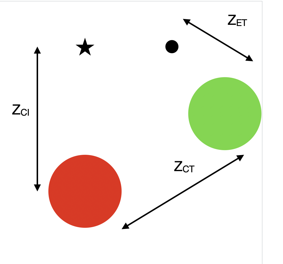
Figure 3: A schematic diagram of more typical results of current GBS experiments, with color codes as in Fig (2). For this more realistic case, one has $Z_{ET}>1$, giving a poor fit to a thermalized model, but the classical model is even worse, such that $Z_{CT}\gg 1$. We emphasize that other, more efficient classical algorithms may exist, which could alter these comparisons.

An interesting open question in computer science, not treated here, is whether all efficient (not exponentially slow) classical fakes can be identified using the multiple statistical tests that we have identified in this paper.

Our results highlight the importance of scalable validation methods for experimental data in current technologies. These algorithms provide techniques for validating large experiments. Scalability requirements and computability are fundamental to any theory that describes high-order multi-mode experiments. This includes Bose-Einstein condensates [42], dynamical phase-transitions [43], noisy quantum computers [44], random quantum circuits [45], multi-qubit photon-atom interactions [46], coherent Ising machines (CIM) [25, 30], and many others now under experimental development.

In summary, grouped count probabilities simulated in phase-space can be used to compare the experimental correlations of large-scale Gaussian boson sampling experiments with quantum theoretical predictions. We distinguish the experimental data from some types of classically generated data. This is carried out using a statistical distance $Z$, normalized by the sampling errors. High order correlations give the strongest tests. There is substantial disagreement between experiment and the idealized GBS model. However, evidence does exist for quantum advantage from the high-order correlations, provided the target computational distribution is slightly decoherent.

II Phase-space representations of bosonic networks

We first summarize results presented previously [23, 24] on representing the input and output states of a bosonic network with phase-space methods. Such representations are a natural fit for describing bosonic networks with Gaussian inputs. They are inherently scalable and have analytical expressions which are simple to implement numerically.

They are also applicable to other quantum technologies with nonlinearities and feedback, like the CIM [47, 25, 48, 49]. To simulate quantum inputs, we focus on the generalized P-representation [50], Wigner representation [51, 52] and Q-function [53] which can all give positive, non-singular distributions for squeezed state inputs.

Choosing a representation that minimizes computational sampling errors is of paramount importance. We will show that the normally ordered positive-P method is the preferred choice for GBS photon-counting experiments, due to its low sampling errors for high-order correlations, as shown in Section (III.1).

II.1 Input state

Linear networks are conceptually very simple. Without losses, the network itself is represented by a $M\times M$ Haar random unitary matrix $\boldsymbol{U}$ [1, 2, 16, 54], however losses cause the network to become non-unitary. Therefore, a lossy network is denoted by the $M\times M$ transmission matrix $\boldsymbol{T}$. Out of $M$ total input channels, $N\subset M$ are filled with input states, which are then converted to $M$ outputs via the linear network.

II.1.1 Pure squeezed states

In an ideal GBS experiment, the inputs are independent Gaussian single-mode squeezed states, allowing one to write the input state as $\hat{\rho}^{(\text{in})}=\prod_{j}\left|\boldsymbol{r}\right\rangle\left\langle\boldsymbol{r}\right|$, where $\boldsymbol{r}=\left[r_{1},\dots,r_{N}\right]$ is the squeezing vector. Ideally, these inputs are pure squeezed states, which are nonclassical minimum uncertainty states defined entirely by their quadrature variances [55, 56, 57].

Following standard quantum optics techniques [58], the non-vanishing quadrature correlations are

$$\left\langle\left(\Delta\hat{x}_{j}\right)^{2}\right\rangle =2\left(n_{j}+m_{j}\right)+1=e^{2r_{j}}$$

$$\left\langle\left(\Delta\hat{y}_{j}\right)^{2}\right\rangle =2\left(n_{j}-m_{j}\right)+1=e^{-2r_{j}}.$$ (1)

Here, $\hat{x}_{j}=\hat{a}_{j}+\hat{a}_{j}^{\dagger}$, $\hat{y}_{j}=\left(\hat{a}_{j}-\hat{a}_{j}^{\dagger}\right)/i$ are the quadrature operators which obey the commutation relation $\left[\hat{x}_{j},\hat{y}_{k}\right]=2i\delta_{jk}$, while $n_{j}=\sinh^{2}(r_{j})$ and $m_{j}=\cosh(r_{j})\sinh(r_{j})$ are the input photon number and coherence per mode, respectively.

From the Heisenberg uncertainty principle, this allows one to write the requirement for a minimum uncertainty ideal squeezed state as

$$\left\langle\left(\Delta\hat{x}_{j}\right)^{2}\right\rangle\left\langle\left(\Delta\hat{y}_{j}\right)^{2}\right\rangle=1.$$ (2)

II.1.2 Thermalized squeezed states

Experimentally generating pure squeezed states is challenging. Laboratory equipment such as lasers, polarizing beamsplitters, mirrors and phase-shifters will inevitably introduce decoherence due to laser noise, temporal drift, refractive index fluctuations [59], mode mismatch [17] and dephasing effects [60].

This means that the squeezed states can no longer be considered pure, and realistically one has $\left\langle\left(\Delta\hat{x}_{j}\right)^{2}\right\rangle\left\langle\left(\Delta\hat{y}_{j}\right)^{2}\right\rangle>1$. Therefore, to accurately model an experimental implementation of bosonic networks, one needs to account for this additional decoherence, even though it is generally not included in the reported experimental data. We do this by fitting the reported data to a model for thermalized squeezed states [37], together with a correction to the transmission matrix [23].

We suppose that a beamsplitter attenuates the input intensity by a factor of $1-\epsilon$, while adding $n_{j}^{th}=\epsilon n(r_{j})$ thermal photons per mode. This alters the input coherence as $\tilde{m}_{j}=\left(1-\epsilon\right)m(r_{j})$, whilst keeping the input photon number unchanged. The advantage of this model is that one can easily test a variety of input states from thermal, $\epsilon=1$, to pure squeezed states, $\epsilon=0$, and anything in between, by simply changing $\epsilon$. Because this changes the resulting count distribution, we improve the fit to the reported data by including a correction factor $t$ to the transmission matrix.

Since squeezed states can be modeled using a variety of phase-space methods, it is useful to employ operator-ordering methods for such simulations. The most convenient method uses the amount of vacuum noise added with each representation to define a corresponding operator ordering parameter $\sigma$, which is similar to $s$-ordering [61]. Here, $\sigma=0$ denotes normal ordering, $\sigma=1/2$ symmetric ordering and $\sigma=1$ anti-normal ordering.

Using this ordering method, the squeezed quadrature variance with the above beamsplitter model of decoherence in any representation is defined as

$$\left\langle\left\{\left(\Delta\hat{x}_{j}\right)^{2}\right\}_{\sigma}\right\rangle =\Delta_{\sigma x_{j}}^{2}=2\left(n_{j}+\sigma+\tilde{m}_{j}\right)$$

$$\left\langle\left\{\left(\Delta\hat{y}_{j}\right)^{2}\right\}_{\sigma}\right\rangle =\Delta_{\sigma y_{j}}^{2}=2\left(n_{j}+\sigma-\tilde{m}_{j}\right).$$ (3)

For compact notation, we may omit the $\sigma$ in subscripts when it is zero, for normal ordering.

II.2 Glauber-Sudarshan P-representation

To simulate linear networks in phase-space, one is restricted by both the input state and the type of detector used. If normally ordered photo-number-resolving (PNR) detectors are used, any non-normally ordered representation introduces vacuum noise in the initial stochastic samples. We show in Sec. (III.1) that this causes a rapid growth of computational sampling errors when computing high-order intensity correlations.

We first summarize results for the diagonal Glauber-Sudarshan P-representation, which is defined in terms of the density matrix [62, 63] using coherent states $\left|\boldsymbol{\alpha}\right\rangle$, as:

$$\hat{\rho}=\int P(\boldsymbol{\alpha})\left|\boldsymbol{\alpha}\right\rangle\left\langle\boldsymbol{\alpha}\right|\text{d}^{2}\boldsymbol{\alpha}.$$ (4)

This normally-ordered phase-space representation can have singular distributions for general quantum states, including squeezed and number states. However, it is always positive for thermal and coherent states [56, 64]. More generally, classical states are defined as having a positive diagonal P-representation, so that no quadrature has a variance below that of the vacuum state [36, 65].

II.2.1 Classical states

Because they generate discrete counts that are classically stimulable, classical states have been analyzed to verify experiments indeed send $N$ quantum states into the linear network. Large amounts of decoherence in the inputs may cause the input state to become classical, allowing the resulting output distribution to be efficiently simulated on a classical computer [65, 66].

An extreme case is a thermal state, which is a fully decoherent classical state with normally-ordered quadrature variance

$$\left\langle\left(\Delta\hat{x}_{j}\right)^{2}\right\rangle=\left\langle\left(\Delta\hat{y}_{j}\right)^{2}\right\rangle=2n_{j},$$ (5)

obtained by letting $\epsilon=1$ in Eq.(3).

Simulations of $N\subset M$ thermal states sent into a linear network have been performed previously [17, 18] and shown to not accurately model any recent experimental implementations of GBS [17, 18, 19].

A more realistic state is a classical approximation to pure squeezed states called squashed states [38, 39]. These states arise as the classical limit of thermalized squeezed states with $\epsilon=\lim_{r_{j}\rightarrow\infty}(1-\tanh(r_{j}))$, corresponding to $m_{j}=n_{j}$. Unlike thermal states, squashed states maintain the squeezed quadrature variance condition

$$\left\langle\left(\Delta\hat{x}_{j}\right)^{2}\right\rangle\neq\left\langle\left(\Delta\hat{y}_{j}\right)^{2}\right\rangle,$$ (6)

however, neither quadrature is squeezed below the vacuum noise limit. From Eq.(1) the normally ordered variance is defined as [38, 39]:

$$\left\langle\left(\Delta\hat{x}_{j}\right)^{2}\right\rangle =4n_{j}+1$$

$$\left\langle\left(\Delta\hat{y}_{j}\right)^{2}\right\rangle =1.$$ (7)

Although squashed states contain no true squeezing as one quadrature has fluctuations at the vacuum limit, squashed states present a more realistic classical input state compared to the fully decoherent thermal states.

Recently, simulations of squashed states input to the $100$-mode bosonic network of Zhong et al [17] were shown to be closer to the experimental output distributions than the theoretical ideal GBS distribution [39]. However the same simulations performed for the $144$-mode network of Zhong et al [17] produced mixed results, as outlined in more detail in section VI.

Although the diagonal P-representation is unsuitable for simulating networks with squeezed state inputs, it is well suited to simulate networks with classical inputs [66, 65]. This is demonstrated in section VI for squashed states which are also used to generate fake binary patterns.

The detailed form of the distribution is given in the next subsection.

II.3 Wigner and Q representations

For $\sigma\geq 1/2$ one finds that a classical phase-space is always sufficient to obtain a non-negative Gaussian distribution, even for squeezed states. This leads to the symmetrically ordered Wigner representation ($\sigma=1/2$) and anti-normally ordered Q-function ($\sigma=1$), which are other alternatives. Both are defined on a classical phase-space and generate a positive distribution for any Gaussian input state.

For Gaussian states, the Wigner distribution can be written in the simple form [67, 68, 58]

$$W\left(\boldsymbol{\alpha}\right)=\frac{1}{\pi^{2N}}\int\text{d}^{2}\boldsymbol{\mathrm{z}}\text{Tr}\left\{\hat{\rho}e^{i\boldsymbol{\mathrm{z}}\cdot\left(\hat{\boldsymbol{\mathrm{a}}}-\boldsymbol{\alpha}\right)+i\boldsymbol{\mathrm{z}}^{*}\cdot\left(\hat{\boldsymbol{\mathrm{a}}}^{\dagger}-\boldsymbol{\alpha}^{*}\right)}\right\},$$ (8)

where $\text{Tr}\{\dots\}$ is a trace and $\boldsymbol{\mathrm{z}}$ is a complex vector, while the Q-function is written in the standard form [53]:

$$Q\left(\boldsymbol{\alpha}\right)=\frac{1}{\pi^{N}}\left\langle\boldsymbol{\alpha}\mid\hat{\rho}\mid\boldsymbol{\alpha}\right\rangle.$$ (9)

These representations have been used previously to obtain analytical expressions for the probability of a specific GBS output pattern [2, 16, 3] and to determine the classical simulability of noisy GBS networks [66]. We use the notation $P_{\sigma}$ to indicate any distribution of this type over a classical phase-space.

In all cases, we define classical quadrature phase-space variables as:

$$x_{j} =\alpha_{j}+\alpha_{j}^{*}\sim\hat{x}_{j},$$

$$y_{j} =\left(\alpha_{j}-\alpha_{j}^{*}\right)/i\sim\hat{y}_{j}.$$ (10)

Any thermalized squeezed vacuum state with non-negative variances $\Delta_{\sigma x_{j}}^{2}$ , $\Delta_{\sigma y_{j}}^{2}$ has a non-singular, Gaussian distribution on a classical phase-space, with

$$P_{\sigma}(\boldsymbol{\alpha})=\prod_{j}\left(\frac{2}{\pi\Delta_{\sigma x_{j}}\Delta_{\sigma y_{j}}}e^{-x_{j}^{2}/2\Delta_{\sigma x_{j}}^{2}-y_{j}^{2}/2\Delta_{\sigma y_{j}}^{2}}\right).$$ (11)

Using the $\sigma$-ordering scheme, the equivalence between operator moments and stochastic moments is given by the $\sigma$-ordering relation:

$$\left\langle\left\{\hat{a}_{j_{1}}^{\dagger},\ldots,\hat{a}_{j_{n}}\right\}_{\sigma}\right\rangle =\left\langle\alpha_{j_{1}}^{*},\ldots,\alpha_{j_{n}}\right\rangle_{\sigma}$$

$$=\int P_{\sigma}(\boldsymbol{\alpha})\left[\alpha_{j_{1}}^{*},\ldots,\alpha_{j_{n}}\right]\text{d}^{2M}\bm{\alpha}.$$ (12)

where $\left\{\dots\right\}_{\sigma}$ and $\left\langle\dots\right\rangle_{\sigma}$ denotes $\sigma$-ordered operator products and stochastic averages, respectively.

Representations with $\sigma\geq 1/2$ introduce vacuum noise in the initial stochastic samples when used to analyze photon-number detectors. The additional noise makes the Wigner and Q representations completely impractical for any computation of high-order correlations in current large-scale bosonic networks that use photon-number detectors.

We show below that the added vacuum noise causes an exponential increase in sampling error with $M$, for high-order correlations.

II.4 Positive P-representation

The generalized P-representation is a normally ordered distribution in phase-space that is exact and non-singular for any input quantum state. This is useful for simulating the correlations of squeezed or number states, as it doesn’t introduce vacuum noise.

The representation is written as

$$\hat{\rho}=\int\int P\left(\boldsymbol{\alpha},\boldsymbol{\beta}\right)\hat{\Lambda}\left(\boldsymbol{\alpha},\boldsymbol{\beta}\right)\text{d}\mu\left(\boldsymbol{\alpha},\boldsymbol{\beta}\right),$$ (13)

where $\hat{\rho}$ is expanded over a subspace of the complex plane, $\boldsymbol{\alpha},\boldsymbol{\beta}$ are independent coherent state amplitude vectors [69] and

$$\hat{\Lambda}\left(\boldsymbol{\alpha},\boldsymbol{\beta}\right)=\frac{\left|\boldsymbol{\alpha}\right\rangle\left\langle\boldsymbol{\beta}^{*}\right|}{\left\langle\boldsymbol{\beta}^{*}\mid\boldsymbol{\alpha}\right\rangle}$$ (14)

is the off-diagonal coherent state projector. If $P\left(\boldsymbol{\alpha},\boldsymbol{\beta}\right)=P\left(\boldsymbol{\alpha}\right)\delta\left(\boldsymbol{\alpha}^{*}-\boldsymbol{\beta}\right)$, this reduces to the Glauber-Sudarshan representation where $\boldsymbol{\beta}=\boldsymbol{\alpha}^{*}$ defines a classical phase-space.

The projection operator projects the density matrix onto multi-mode coherent states. This is responsible for the exact and non-singular nature of the generalized-P distribution for quantum inputs as it doubles the classical phase-space dimension, which allows off-diagonal coherent state amplitudes with $\boldsymbol{\beta}\neq\boldsymbol{\alpha}^{*}$ to exist in the basis. These represent nonclassical quantum superposition states [50, 70].

The generalized P-representation is a family of normally ordered representations with different distributions $P\left(\boldsymbol{\alpha},\boldsymbol{\beta}\right)$, the form of which is dependent on the integration measure $\text{d}\mu\left(\boldsymbol{\alpha},\boldsymbol{\beta}\right)$ [50]. Here, we use the positive P-representation, which is obtained when $\text{d}\mu\left(\boldsymbol{\alpha},\boldsymbol{\beta}\right)=\text{d}^{2M}\boldsymbol{\alpha}\text{d}^{2M}\boldsymbol{\beta}$, which is a $4M$-dimensional volume integral, and $\boldsymbol{\alpha},\boldsymbol{\beta}$ can vary along the whole complex plane. By taking the real part of Eq.(13), the density matrix becomes hermitian and can be sampled efficiently.

Because it gives an efficiently sampled, non-singular and strictly positive output distribution in all cases, the positive P-representation is ideal for simulating bosonic networks with squeezed state inputs. It combines probabilistic properties with operator normal-ordering, giving a one-to-one relationship between normally-ordered operator moments and stochastic moments [40]:

$$\left\langle\hat{a}_{j_{1}}^{\dagger},\ldots,\hat{a}_{j_{n}}\right\rangle=\left\langle\beta_{j_{1}},\ldots,\alpha_{j_{n}}\right\rangle_{P}.$$ (15)

This relationship is valid for any generalized P-representation, where $\left\langle\dots\right\rangle$ denotes a quantum expectation value and $\left\langle\dots\right\rangle_{P}$ is a generalized-P average.

For a pure squeezed state, the input state density matrix $\hat{\rho}^{(\text{in})}$ can be written in terms of the positive-P distribution by expanding each squeezed state $\left|\boldsymbol{r}\right\rangle$ as a line integral over a real coherent state [71], so that $\text{d}\mu\left(\boldsymbol{\alpha},\boldsymbol{\beta}\right)=\text{d}\boldsymbol{\alpha}\text{d}\boldsymbol{\beta}$, with $\boldsymbol{\alpha},\boldsymbol{\beta}$ as independent real vectors. Alternatively, one can view this as a distribution over the $4M$ dimensions of the full phase-space, with delta-function distributions on the $2M$ imaginary axes.

This gives

$$\hat{\rho}^{(\text{in})}=\text{Re}\int\int P\left(\boldsymbol{\alpha},\boldsymbol{\beta}\right)\hat{\Lambda}\left(\boldsymbol{\alpha},\boldsymbol{\beta}\right)\text{d}\boldsymbol{\alpha}\text{d}\boldsymbol{\beta}.$$ (16)

Here

$$P\left(\boldsymbol{\alpha},\boldsymbol{\beta}\right)=\prod_{j}C_{j}e^{-\left(\alpha_{j}^{2}+\beta_{j}^{2}\right)\left(\gamma^{-1}+1/2\right)+\alpha_{j}\beta_{j}}$$ (17)

is a positive-P distribution for an input pure squeezed state, which is a Gaussian distribution on a positive $\alpha,\beta$ plane, where $C_{j}$ is the normalization constant and $\gamma_{j}=e^{2r_{j}}-1=2\left(n_{j}+m_{j}\right)$. To diagonalize this Gaussian, we take $x_{j}=\alpha_{j}+\beta_{j}\sim\hat{x}_{j}$, $\bar{y}_{j}=\alpha_{j}-\beta_{j}\sim i\hat{y}_{j}$ as real variables, with the result that each is now an independent Gaussian, with

$$\Delta_{x_{j}}^{2} =2\left(n_{j}+m_{j}\right)$$

$$\Delta_{\bar{y}_{j}}^{2} =2\left(m_{j}-n_{j}\right).$$ (18)

This variable change gives the expansion as:

$$P\left(\boldsymbol{\alpha},\boldsymbol{\beta}\right)=\prod_{j}\left(\frac{2}{\pi\Delta_{x_{j}}\Delta_{\bar{y}_{j}}}e^{-x_{j}^{2}/2\Delta_{x_{j}}^{2}-\bar{y}_{j}^{2}/2\Delta_{\bar{y}_{j}}^{2}}\right).$$ (19)

So far, we have assumed the squeezing orientation $\left\langle:\left(\Delta\hat{x}_{j}\right)^{2}:\right\rangle>0$ and $\left\langle:\left(\Delta\hat{y}_{j}\right)^{2}:\right\rangle<0$, as it is for a pure squeezed state. Since one of the normally-ordered variances is always negative, the phase-space variable corresponding to the hermitian $\hat{y}$ operator is imaginary, which requires that $\alpha^{*}\neq\beta$. Hence, we have a nonclassical phase-space.

This result can be extended to thermalized cases by modifying the variances, as long as $\left\langle:\left(\Delta\hat{y}_{j}\right)^{2}:\right\rangle<0$. If thermalization is stronger, with $\left\langle:\left(\Delta\hat{y}_{j}\right)^{2}:\right\rangle\geq 0$, then the integration domain is changed so that $\beta=\alpha^{*}$. This reduces to the Glauber-Sudarshan classical case already treated.

II.5 Gaussian sampling in $\sigma$-ordered representations

The above results can be combined to give a unified random sampling expression valid in the case of any Gaussian input. We can construct initial stochastic samples, which are valid for any ordering $\sigma$, as [60]

$$\alpha_{j} =\frac{1}{2}\left(\Delta_{\sigma x_{j}}w_{j}+i\Delta_{\sigma y_{j}}w_{j+M}\right)$$

$$\beta_{j} =\frac{1}{2}\left(\Delta_{\sigma x_{j}}w_{j}-i\Delta_{\sigma y_{j}}w_{j+M}\right),$$ (20)

where $\left\langle w_{j}w_{k}\right\rangle=\delta_{jk}$ are real Gaussian noises. For a squeezed $y$-quadrature with normal ordering where $\Delta_{y_{j}}$ is imaginary, $\alpha_{j}$ and $\beta_{j}$ are real and independent. This holds even for impure states. For cases where $\Delta_{\sigma y_{j}}$is real, either because of thermalization or because the ordering has $\sigma\geq 1/2$, $\alpha_{j}$ and $\beta_{j}$ are complex conjugate.

This sampling method is able to generate any Gaussian state with no cross-correlations between the $\hat{x}$ and $\hat{y}$ quadratures, which are generically thermalized squeezed states. If there is no squeezing below the vacuum level, this representation reduces to the classical-like Glauber P-representation for normal ordering.

It is possible that even more sophisticated models are needed to fully explain the current experimental observations, as explained below, but that is outside the scope of the present paper.

II.6 Output density matrix

Practically, linear networks consist of a series of polarizing beamsplitters and mirrors, causing the $N$ input modes to interfere, generating large amounts of entangled states, and converting the input state to the output state $\hat{\rho}^{(\text{out})}$.

In terms of phase-space distributions, this corresponds to transforming the initial stochastic amplitudes as $\boldsymbol{\alpha}^{\prime}=\boldsymbol{T}\boldsymbol{\alpha}$ and $\boldsymbol{\beta}^{\prime}=\boldsymbol{T}^{*}\boldsymbol{\beta}$, which is valid for all representations, provided there are no losses. In the normally ordered case, the resulting output density matrix for nonclassical inputs can therefore be sampled as before, but with a transformed projector:

$$\hat{\rho}^{(\mathrm{out})}=\text{Re}\int\int P(\bm{\alpha},\bm{\beta})\hat{\Lambda}\left(\bm{T}\bm{\alpha},\bm{T}^{*}\bm{\beta}\right)\mathrm{d}\mu\left(\bm{\alpha},\bm{\beta}\right).$$ (21)

To take into account losses and detector inefficiencies, one can include a larger unitary with loss channels, but only consider the sub-matrix of $\bm{T}$ for the channels that are measured. For example, in the matrix $\bm{T}=t\bm{U}$, all channels experience equal loss where $t$ is an amplitude transmission coefficient. Due to the normal ordering property of the any P-representation, this method remains exactly equivalent to using a master equation method to treat losses. However, non-normally ordered methods require extra noise terms if there are losses [24, 23].

Thermal noise or other random processes can also be included if present. For cases in which $n^{th}>0$ in the loss reservoirs or $\sigma>0$ one must include these additional quantum or thermal noise terms with losses. Such terms correspond to $\sigma$-ordered noise in the reservoir modes. For the results given here, we assume that thermal noise only occurs in the input modes, and that the reservoirs are at zero temperature, which is a good approximation in optical experiments.

III Grouped Correlation probabilities

Correlations provide a signature of measurable quantum states. For these to be a useful signature, they must be readily observable, relevant to interesting quantum features, and have a low enough sampling error to provide an unambiguous result. In this section, we review both Glauber intensity correlations and GCPs of bosonic networks, which have already been successfully used to compare theory and experiment for an $M=100$ mode GBS experiment [23].

III.1 Intensity correlations

The most commonly used correlation in quantum optics is the $n$-th order Glauber intensity correlation [69]. In photonic experiments with PNR detectors [72, 73, 74, 41], the expectation value of the product of normally ordered output number operators in a set of up to $M$ output modes is observed:

$$G^{(n)}(c_{j})=\left\langle:(\hat{n}^{\prime}_{j})^{c_{j}}\dots\>(\hat{n}^{\prime}_{M})^{c_{M}}:\right\rangle,$$ (22)

where $\hat{n}^{\prime}_{j}=\hat{a}_{j}^{\dagger\text{(out)}}\hat{a}_{j}^{\text{(out)}}$ is the output photon number operator, while $c_{j}=0,1,2,\dots$ is the number of photon counts at the $j$-th detector, and $n=\sum c_{j}$ is the correlation order.

In the positive-P phase-space representation, output correlations are obtained by computing moments which, due to the equivalence of operator and stochastic moments, are obtained simply by replacing $\hat{n}^{\prime}_{j}$ with $n^{\prime}_{j}=\alpha^{\prime}_{j}\beta^{\prime}_{j}$, such that for a large number of samples

$$G^{(n)}=\left\langle(n^{\prime}_{j})^{c_{j}}\dots\>(n^{\prime}_{M})^{c_{M}}\right\rangle_{0}.$$ (23)

In the $\sigma$-ordered phase-space case, the required reordering of all number operators produces a correction term which must be included to remove the vacuum noise introduced by each operator. Provided $c_{j}=0,1$, this correction allows the stochastic variable to become equivalent to the normally ordered output particle number, when $\boldsymbol{T}$ is unitary, via the replacement

$$n^{\prime}_{j}=\alpha^{\prime}_{j}\beta^{\prime}_{j}-\sigma.$$ (24)

In principle, $c_{j}$ is arbitrary but is limited to $c_{j}=0,1$ for simple cross-correlations of photon-number resolved detectors. For more general cases of higher order moments and correlations with $c_{j}>1$ the non-normally-ordered expressions become cumbersome, and are not listed here.

This in itself may not be a severe limitation, as GBS proposals with PNR detectors often assume the probability of observing more than one photon at a detector is small [2, 16]. However, as shown in Fig (4), the computational sampling error of Wigner and Q-function simulations grows rapidly with correlation order, making them unsuitable for generating moments to compare with experiment.

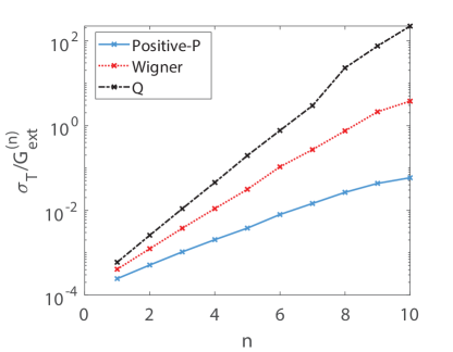
Figure 4: Comparison of sampling error growth for an $M=20$, $N=20$ GBS with uniform pure squeezed state inputs and $E_{S}=4.8\times 10^{7}$ samples. The ratio of theoretical sampling errors, $\sigma_{T}$, with an exactly computed n-th order intensity correlation, $G_{ext}^{(n)}$, is plotted. Q-function simulations are denoted by the dashed black line, and add the largest amount of vacuum noise per photon number. The Wigner representation simulations are denoted by the red dotted line, which adds half a quantum of noise per photon number, whilst the positive-P representation adds no vacuum noise and corresponds to the solid blue line, with far lower sampling error. Details are given in Section (IV).

For cases with sufficiently low flux corresponding to small mean photon numbers, threshold detectors are equivalent to PNR detectors. Therefore, intensity correlations are also the probability of an $N$-fold coincidence count $P_{N}$. This allows one to write the correlation as a simple product of output number operators, such that

$$P_{N}\equiv\left\langle\prod_{j}\hat{n}^{\prime}_{j}\right\rangle.$$ (25)

At high flux levels, a single PNR detector may register more than one count and the output is no longer binary. In such cases, we must distinguish between PNR and threshold detectors. To get accurate results for threshold detectors, a different operator is used.

III.2 Grouped count correlations for saturating detectors

To date, multiple GBS experiments of large scale networks have been conducted using both PNR detectors [19], and threshold, or click, detectors which saturate for more than one count at a detector [17, 18]. When PNR detectors are used, one samples from the Hafnian distribution [2, 16], whilst threshold detectors are equivalent to sampling from the Torontonian distribution [3].

We focus on experiments using the latter detector type, with outputs being binary numbers where the $j$-th detector records $c_{j}=1$ for a photon detection event, or click, and $c_{j}=0$ for no detection event. Therefore, a network of $M$ detectors will produce binary patterns represented by the count vector $\boldsymbol{c}$, with $2^{M}$ possible patterns available. Each detector is defined by the normally-ordered projection operator [75]

$$\hat{\pi}_{j}\left(c_{j}\right)=:e^{-\hat{n}^{\prime}_{j}}\left(e^{\hat{n}^{\prime}_{j}}-1\right)^{c_{j}}:.$$ (26)

The expectation of this for $c_{j}=1$ is the first-order click correlation moment, $\left\langle\hat{\pi}_{j}\left(1\right)\right\rangle$, which is the probability of observing a click at the $j$-th detector. The projection operator for a specific binary pattern $\boldsymbol{c}$ is $\hat{\Pi}\left(\bm{c}\right)=\bigotimes_{j=1}^{M}\hat{\pi}_{j}\left(c_{j}\right)$, whose expectation value is the Torontonian function [3]. This is exponentially small in almost all cases, which means it cannot be measured for large scale experiments due to experimental sampling errors.

To compute output probabilities of bosonic networks with threshold detectors without directly generating discrete patterns we use grouped count probabilities (GCPs). These generate moments of multiple possible output patterns. They also allow one to carry out exponentially many high-order correlation tests.

A GCP computes the probability of observing $\boldsymbol{m}=\left(m_{1},\dots,m_{d}\right)$ grouped counts in $d$-dimensions. Each grouped count $m_{j}$ is obtained by summing over all binary patterns. These are combined into bins based on the number of detector counts in a subset $S_{j}$ of all $M$ output modes, such that $m_{j}=\sum_{i}^{M}c_{i}$. A $d$-dimensional GCP is therefore defined as [23]

$$\mathcal{G}_{\boldsymbol{S}}^{(n)}\left(\boldsymbol{m}\right)=\left\langle\prod_{j=1}^{d}\left[\sum_{\sum c_{i}=m_{j}}\hat{\Pi}_{S_{j}}\left(\boldsymbol{c}\right)\right]\right\rangle,$$ (27)

where $n=\sum_{j=1}^{d}M_{j}\leq M$ is the total click correlation order, following Glauber’s definition [69], and $\boldsymbol{S}=\left(S_{1},S_{2},\dots\right)$ is the vector of disjoint subsets of $\boldsymbol{M}=\left(M_{1},M_{2},\dots\right)$ output modes. These includes marginal probabilities where some detectors are not monitored, as well as moments like the Torontonian. However, a GCP has the advantage of being both measurable and including data from all detectors if required.

III.2.1 Numerical computation

As well as being unmeasurable, the Torontonian is not computable at large scale. There are no efficient direct techniques, and phase-space methods are only useful where the Torontonian has a large enough value to exceed the theoretical sampling error. However, many GCPs are both measurable and computable, as they are easily computed using the positive-P representation.

Due to the operator equivalence Eq.(15), the the normally ordered projection operator $\hat{\pi}_{j}$ is computed via a replacement with the positive-P observable

$$\pi_{j}=e^{-n^{\prime}_{j}}\left(e^{n^{\prime}_{j}}-1\right)^{c_{j}},$$ (28)

where $n^{\prime}_{j}$ is sampled from the output distribution Eq.(21).

The summation over detector outputs is efficiently carried out using the multi-dimensional inverse discrete Fourier transform [23]

$$\mathcal{G}_{\boldsymbol{S}}^{(n)}\left(\boldsymbol{m}\right)=\frac{1}{\prod_{j}(M_{j}+1)}\sum_{\boldsymbol{k}}\tilde{\mathcal{G}}_{M}^{(n)}(\boldsymbol{k})e^{i\sum_{j}k_{j}\theta_{j}m_{j}},$$ (29)

where

$$\mathcal{\tilde{G}}_{\boldsymbol{S}}^{(n)}\left(\boldsymbol{k}\right)=\left\langle\prod_{j=1}^{d}\bigotimes_{i\in S_{j}}\left(\pi_{i}(0)+\pi_{i}(1)e^{-ik_{j}\theta_{j}}\right)\right\rangle_{P},$$ (30)

is the Fourier observable, $\theta_{j}=2\pi/(M_{j}+1)$ is the Fourier angle, $k_{j}=0,\dots,M_{j}$ and $j=1,\dots,d$ defines the dimension.

The Fourier transform is not only numerically efficient and highly scalable, but allows all possible correlations present in the network to be simulated, removing all patterns that don’t contain $\boldsymbol{m}$ counts.

III.2.2 Multi-dimensional binning of grouped correlations

The experimentally reported total count probability [17, 18], which is the probability of observing $m$ clicks in any pattern, is typically one of the first comparison tests experimental samples are subjected to. It allows one to quickly determine whether outputs are close to the expected distribution obtained using pure squeezed state inputs, typically called the ’ideal’ or ’ground truth’ distribution in the literature.

However, Villalonga et al [34] has shown that total count distributions can be spoofed by classical algorithms which sample from low-order marginal probabilities. Their second and third-order samplers generate distributions that are closer to the theoretical ideal distribution, approximated as a Gaussian in the limit of large numbers of clicks, than an experiment which has claimed quantum advantage [18]. Therefore, comparison tests are needed which utilize the true high-order correlations generated in a linear network, to help differentiate output distributions from experiments and classical sampling algorithms.

This is where grouped probabilities with dimension $d>1$ become particularly useful for statistical comparisons. A $d>1$-dimensional grouped correlation of order $n=M$ is the probability of observing $m_{1},\dots,m_{d}$ grouped counts in the subsets

$$\boldsymbol{S}=\left(S_{1},\dots,S_{d}\right)=\left(\{1,\dots,M/d\},\dots,\{M/d+1,\dots M\}\right),$$ (31)

such that $m_{1}=\sum_{i=1}^{M/d}c_{i}$, $m_{d}=\sum_{i=M/d+1}^{M}c_{i}$.

The increased dimension means high-order correlations present in the data become more statistically significant. This has two fundamental benefits over one-dimensional comparisons; First, the increased dimension generates a larger number of bins, or data points, that are available for statistical testing. The number of bins generated per dimension scales as $(M/d+1)^{d}$, although only a subset of these are used for statistical testing (see Appendices).

This allows a fine tuned comparison of theoretical and experimental outputs. If statistical tests show discrepancies increase as dimension increases, even after simple decoherence effects are included, this could indicate further imperfections are affecting the network.

Second, multi-dimensional GCPs simulated in phase-space provide an efficient method for differentiating between data spoofed by low-order sampling algorithms [34, 35] and data generated from quantum experiments. This is due to such spoofing algorithms generating patterns with an inherent bias as spoofing high-order correlations generated in large size experiments is computationally challenging for low-order sampling algorithms.

Additional tests can be performed by randomly permuting each binary pattern. This changes the output modes contained within each subset $S_{j}$, leading to different values of $m_{j}$ for each permutation. Without repetitions, there are

$$\frac{\binom{M}{M/d}}{d}=\frac{M!}{d(M/d)!(M-M/d)!},$$ (32)

possible ways of computing $m_{1},\dots,m_{d}$.

This produces exponentially many non-trivial, randomized high-order tests when $d>1$, allowing exponentially many comparisons to take place, with different high-order correlations being observed in each test.

If repeated comparisons show differences between theoretical and experimental outputs remain statistically significant, one can hypothesize experimental imperfections are causing samples to become inaccurate. These random permutation tests can be simulated efficiently by applying the same permutation used on the experimental samples to the rows of the transmission matrix $\boldsymbol{T}$ used in the phase-space simulation.

Theoretically, one can bin counts up to the maximum dimension possible of $d=M$, which corresponds to the Torontonian. However, this is strongly restricted by experimental sampling errors which increase with dimension $d$ due to each bin containing progressively fewer photon counts.

III.2.3 Low-order click correlations

Low-order marginal probabilities compute correlations over $n$ output modes whilst ignoring the other $M-n$ modes [76, 77], with the number of observable correlations scaling as $\binom{M}{n}$. For click detectors, the first and second-order click correlations are defined as $\left\langle\hat{\pi}_{j}(1)\right\rangle$ and $\left\langle\hat{\pi}_{j}(1)\hat{\pi}_{k}(1)\right\rangle$, respectively.

The computational efficiency of computing low-order marginals of the ideal output distribution has two advantages for GBS validation; It allows a fast and direct comparison of specific experimental correlations generated from a network with their expected values [18], and has formed foundation of the spoofing algorithms implemented in Ref.[34], which compute the correct connected correlations, also known as cumulants, of the ideal distribution for orders $n\leq 3$.

The first two cumulants are defined as [34, 18, 78]:

$$\kappa_{1} =\left\langle\hat{\pi}_{j}(1)\right\rangle$$

$$\kappa_{2} =\left\langle\hat{\pi}_{j}(1)\hat{\pi}_{k}(1)\right\rangle-\left\langle\hat{\pi}_{j}(1)\right\rangle\left\langle\hat{\pi}_{k}(1)\right\rangle,$$ (33)

and describe the mean click count rate and covariance, respectively. These low-order correlations are used by spoofing algorithms to generate discrete binary patterns for large mode numbers without actually sampling from the full Torontonian distribution.

Computing moments of click correlations is efficient using GCPs simulated in phase-space and is easily illustrated. For example, the third-order click correlation is obtained by setting $n=3$, $S=\{j,k,h\}$ and $\boldsymbol{m}=3$ where $\mathcal{G}_{\{j,k,h\}}^{(3)}(3)=\left\langle\hat{\pi}_{j}(1)\hat{\pi}_{k}(1)\hat{\pi}_{h}(1)\right\rangle$ is the probability of observing clicks at detectors $j,k,h$.

IV Scaling properties

Linear networks produce sampled outputs with random observed photon counts. Statistical testing is vital to determine the accuracy of experimental samples [79]. These statistical comparisons also require an analysis of theoretical sampling errors, which should be comparable or smaller than experimental sampling errors. Hence, the scaling of computational cost or time is determined by the required sample numbers.

Useful comparison simulations for validation and testing purposes must be accurate. In this section, we use Glauber intensity correlations to demonstrate how sampling errors grow with correlation order, illustrating the importance of choosing the correct phase-space representation to simulate bosonic networks with normally ordered detectors. We also give an overview of the statistical estimates used throughout this paper for the experimental and theoretical data.

Details of chi-squared and Z-statistic tests used to compare theory with experiment are given in the Appendices.

IV.1 Experimental sampling errors

We first analyze experimental sampling errors, which are crucial to comparisons of theory and experiment. As the scientific issue is whether theory and experiment agree, we must know what errors exist in the data. We can only conclude there is a difference between theory and experiment if a discrepancy cannot be explained by experimental or theoretical sampling errors.

For any measurement, one would prefer theoretical errors less than the experimental errors. However, there is little to be gained from improving theoretical errors far below experimental errors, which will give negligible additional information about the agreement of theory and experiment. This is also relevant to computational complexity, as explained below.

For the case of measured probabilities $P_{i}^{e}$ of an experimental observation labeled $i$, given $x_{i}$ observations of the event $i$ out of $N_{E}$ experimental samples [80], the estimated probability is obtained as

$$P_{i}^{e}=x_{i}/N_{E}.$$ (34)

For $x_{i}\gg 1$, the variance in $P_{i}^{e}$ is $\sigma_{i}^{2}=P_{i}/N_{E}$, where $P_{i}$ is the true underlying probability.

To understand the scaling issues quantitatively, consider a typical GBS experiment which generates $N_{E}$ random binary numbers $\bm{c}=\left[c_{1},\ldots,c_{M}\right]$. Assuming $\left\langle\hat{\pi}_{j}(1)\right\rangle\approx\left\langle\hat{\pi}_{j}(0)\right\rangle$, there are $2^{M}$ possible outcomes, and in recent large-scale experiments, $2^{M}\gg N_{E}$. Data analyzed here has $N_{E}=4\times 10^{7}$ experimental binary patterns, with the full number of possible outcomes being $2^{144}=10^{43.3}$.

Hence, almost all patterns are never observed, even with $10^{7}$ samples. A rough estimate is that $P_{i}\approx 10^{-43.3}$ for a “typical” pattern. This is the average probability given by the Torontonian function, which is known to be an exponentially hard ($\#P$) function to compute.

However, even in the special cases where it is computable, its not useful for validation. The reason for this is that $x_{i}\gg 1$ is not satisfied, since in almost all cases one has $x_{i}=0$. Even if the theoretical Torontonian could be computed to more than $43$ decimals, and the results stored, the experimental data would have too large an error for useful comparisons. This is the reason why verification requires binning to obtain significant experimental data.

Given a binning method such that there are less than $N_{E}$ distinct outcomes $i$, one can obtain experimental probabilities with a relative error that scales as $1/\sqrt{N_{E}}$. The goal of a theoretical validation is to have an estimate for $P_{i}$ that can reach this level of relative error in the binned Torontonian, even though the Torontonian itself is exponentially hard to compute.

IV.2 Phase-space sampling error

The computational process for simulating phase-space representations is similar for any representation. First, samples $\alpha,\beta$ are generated by randomly sampling the input distribution $E_{S}$ times. For linear networks, the number of initial random numbers required is proportional to $NE_{S}$ with a normally ordered method, or to $ME_{S}$ with non-normally ordered methods, due to the additional algebraic terms which arise from vacuum noise.

If one is interested in dynamical simulations, the samples are then propagated through time to solve a stochastic differential equation [81], the form of which changes depending on the representation, the system Hamiltonian of interest and whether losses are taken into account. However, we are only interested in sampling from the output distribution, which is obtained by transforming the input states as described above.

Regardless of how the initial samples are transformed, output observables are obtained in the form of a stochastic average over the entire ensemble of samples. Therefore, the computation of the product of $E_{S}$ randomly sampled normally ordered output photon numbers $((n^{\prime}_{j})^{c_{j}})^{(k)}$ is

$$\bar{G}^{(n)}=\frac{1}{E_{S}}\sum_{k}^{E_{S}}((n^{\prime}_{j})^{c_{j}})^{(k)}\dots\>((n^{\prime}_{M})^{c_{M}})^{(k)},$$ (35)

where the superscript $k$ denotes the label of a stochastic trajectory in the overall ensemble, and $\bar{G}^{(n)}$ denotes the ensemble mean.

This is valid with all orderings if re-ordered to normal order, provided the appropriate corrections are applied, and there are no correlation terms with $c_{j}>1$. For normal ordering the terms can be repeated, and the result is not restricted to the unitary case, since losses can be included. In other cases, losses require additional noise terms. The other orderings also introduce additional algebraic terms if there are terms with $c_{j}>1$.

Stochastic averages are estimates of the actual theoretical probability obtained from a quantum expectation value of an observed operator. In the limit $E_{S}\rightarrow\infty$, ensemble means converge to the actual theoretical probability such that in the case of Eq.(35), $G^{(n)}=\lim_{E_{S}\rightarrow\infty}\bar{G}^{(n)}$.

Practical implementations of phase-space ensemble averages typically split ensembles into two sub-ensembles, so that $E_{S}=N_{S}N_{R}$ [41]. This has a computational advantage, allowing efficient vector and multi-core parallel computing, and reducing time requirements for large ensemble sizes. There is also a statistical benefit: the first sub-ensemble $N_{S}$ is the number of samples of the initial state. For $N_{S}\rightarrow\infty$, this gives sample averages that are normally distributed via the central limit theorem.

The second sub-ensemble $N_{R}$ is the number of times the computation is repeated. This is equivalent to sampling from a normal distribution $N_{R}$ times [41]. Therefore, the actual computation of the stochastic average Eq.(35) proceeds as

$$\bar{G}^{(n)}=\frac{1}{N_{R}}\sum_{i=1}^{N_{R}}\left(\frac{1}{N_{S}}\sum_{h=1}^{N_{S}}((n^{\prime}_{j})^{c_{j}})^{(h)}\dots\>((n^{\prime}_{M})^{c_{M}})^{(h)}\right)_{(i)},$$ (36)

where $h$, $i$ are the number of samples of the first and second sub-ensembles, respectively.

The second sub-ensemble also generates a statistical estimate of the theoretical sampling error of the ensemble mean as $\sigma_{T}=\sigma_{t}/\sqrt{N_{R}}$, where the sub-ensemble variance is [82, 83]:

$$\sigma_{t}^{2}=\frac{\sum_{i=1}^{N_{R}}\left(\bar{G}_{(i)}^{(n)}-\bar{G}^{(n)}\right)^{2}}{N_{R}-1},$$ (37)

where we define the sub-ensemble mean as the $i$-th sum over the simulated data:

$$\bar{G}_{(i)}^{(n)}=\left(\frac{1}{N_{S}}\sum_{h=1}^{N_{S}}((n^{\prime}_{j})^{c_{j}})^{(h)}\dots\>((n^{\prime}_{M})^{c_{M}})^{(h)}\right).$$ (38)

Thus, the theoretical standard deviation in the mean for $\bar{G}^{(n)}$ is readily obtained from the simulated fluctuations in $\bar{G}_{(i)}^{(n)}$.

A computationally friendly definition of $\sigma_{t}$ can be derived which doesn’t require computing $\bar{G}^{(n)}$ before performing the summation using the expansion $\sum_{i=1}^{N_{R}}\left(\bar{G}_{(i)}^{(n)}-\bar{G}^{(n)}\right)^{2}=\sum_{i=1}^{N_{R}}\left(\bar{G}_{(i)}^{(n)}\right)^{2}-\left(\sum_{i=1}^{N_{R}}\bar{G}_{(i)}^{(n)}\right)^{2}/N_{R}$ [83].

Therefore, when $N_{R}\gg 1$, the theoretical sampling error of the correlation of $E_{S}$ randomly sampled output photon numbers is estimated using the computationally efficient form

$$\sigma_{T}=\sqrt{\frac{\sum_{i=1}^{N_{R}}\left(\left(\bar{G}_{(i)}^{(n)}\right)\right)^{2}-\left(\sum_{i=1}^{N_{R}}\left(\bar{G}_{(i)}^{(n)}\right)\right)^{2}/N_{R}}{N_{R}\left(N_{R}-1\right)}}.$$ (39)

As with any sampling procedure, the sampling error can be reduced by increasing the total number of ensembles which corresponds to increasing either sub-ensemble. Increasing $N_{S}$ requires more memory and processing power, while the speed of an increased $N_{R}$ depends on whether multi-core computing is possible. The more cores available the faster the computation runs.

IV.3 Scaling properties of phase-space sampling errors

To quantify the scaling properties of different phase-space methods, intensity correlations with increasing order are computed using the Wigner, Q and positive-P representations. We consider an $M=20$ mode bosonic network with unit transmission matrix and $N=20$ input pure squeezed states with a uniform squeezing parameter of $\boldsymbol{r}=[1,\dots,1]$. For a network of this type, the output intensity correlations can be computed exactly. Therefore, one can use the ratio of theoretical sampling errors, estimated by Eq.(39), and exactly computed correlations with increasing order to determine how sampling errors of each representation grow with correlation order.

Comparisons are plotted in Fig.(4) for simulations with $E_{S}=4.8\times 10^{7}$ ensembles. The Q and Wigner representations produce sampling errors many orders of magnitude larger than positive-P simulations, and become approximately equal to the computed intensity correlations at orders $n=6$ and $n=8$, respectively. At this point, the numerical sampling error is too large for useful results.

By contrast, the positive-P sampling error is always much smaller, with growth as $n$ increases arising from sampling distributions with decreasing probabilities. These are also increasingly difficult to measure.

This shows the benefit of the normally-ordered approach, which gives exponentially lower error with increasing order compared to other types of ordering. Because we are mostly interested in high-order correlations, we do not use the non-normally ordered methods further.

In earlier work we compared theoretical phase-space simulation errors with expected experimental sampling errors for number-state boson sampling, and found that the theoretical sampling variances are typically much lower than the experimental variances for the same number of samples [41]. This scaling persists in the case of GBS, with detailed results to be given elsewhere.

IV.4 Summary of sampling errors

In summary, it is exponentially hard to estimate probabilities in the unbinned, high order limit, but it is also exponentially hard to measure the probabilities, because in both cases exponentially many samples would be needed. Once the data is binned or marginalized so that it becomes measurable, we find that the positive-P method gives exponentially lower sampling error than other phase-space methods that do not use normal-ordering.

In a previous paper [41], it was shown that the phase-space method also has exponentially lower errors than experiment for identical sample numbers. Hence we are generally able to employ lower numbers of samples than were used in the experiment, which gives a reasonable benchmark for timing comparisons. Apart from this, the timing of the simulations is polynomial, not exponential in the mode number.

V Comparison of theory and experiment

In this section, we compare theoretical GCPs with experimental data from a $144$-mode GBS linear network [18]. This experiment obtained data for two different laser waists, $125\mu m$ and $65\mu m$, and varying laser power. The first waist contains data for two different powers and the second waist, five different powers. Squeezing parameters are $50$-mode vectors of amplitude $\boldsymbol{r}$, one for each laser power tested, while the transmission matrices $\boldsymbol{T}$ are of size $50\times 144$ with two matrices in total, one for each laser waist.

Test statistics for comparisons of GCPs and first-order click correlation moments for all data sets are given, however comparison plots are also only shown for data from laser waist $65\mu m$ and power $1.65W$. This is due to both practicality and claims of computational advantage for this data set, as the cost of computing the Torontonian and generating random outputs scales with the number of modes and hence detector clicks.

This experimental data was compared with an ideal squeezed state model based on the reported experimental parameters, and the thermalized squeezed state model described in Subsection (II.1), with values of $\epsilon,$$t$ chosen to minimize the errors in the total count distributions.

This model does not account for possible inhomogeneities in thermalization for different inputs, nor for inhomogeneities in output transmission or detector efficiency.

Raw data from the tested experiment can be found from [84]. Extracted data used for comparisons in this work, as well as software for generating the phase-space simulations, can be found in the fully open source and documented software package developed for simulating linear bosonic networks with threshold detectors in phase-space, called xQSim, which is available from [85].

V.1 Total count distributions

Waist	Power	Pure squeezed inputs			$t$	$\epsilon$	Thermalized squeezed inputs
		$\chi_{EI}^{2}/k$	$k$	$Z_{EI}$			$\chi_{ET}^{2}/k$	$k$	$Z_{ET}$
$125\mu m$	$1.412W$	$218$	$53$	$78$	$0.9972$	$0.0354$	$2\pm 0.5$	$52$	$4\pm 1.5$
	$0.5W$	$143$	$31$	$50$	$1.0006$	$0.0392$	$20\pm 2$	$31$	$20\pm 1$
$65\mu m$	$1.65W$	$1861$	$85$	$221$	$1.0109$	$0.0428$	$10\pm 1$	$84$	$23\pm 2$
	$1W$	$215$	$74$	$91$	$1.0026$	$0.0354$	$6\pm 1$	$73$	$15\pm 2$
	$0.6W$	$171$	$57$	$72$	$0.9966$	$0.0288$	$2.5\pm 1$	$57$	$6\pm 2$
	$0.3W$	$193$	$40$	$64$	$0.9972$	$0.0202$	$7\pm 1$	$40$	$12\pm 1$
	$0.15W$	$151$	$28$	$49$	$0.9972$	$0.0208$	$1.2\pm 0.3$	$27$	$0.7\pm 1$

Table 1: Statistical test outputs for comparisons of total counts $\mathcal{G}_{144}^{(144)}(m)$ for all data sets obtained from a $144$-mode GBS experiment [18]. Chi-square and approximate Z-statistic tests, defined analytically in the appendix, are generated from comparisons with phase-space simulations of $E_{S}=1.2\times 10^{6}$ ensembles. Comparisons of experiment with simulations of pure squeezed state inputs, the ideal GBS, are denoted by the subscript $EI$, whilst comparisons of simulated thermalized squeezed states are denoted by the subscript $ET$. Parameters $t$ and $\epsilon$ represent corrections to the experimental $\boldsymbol{T}$ matrix and the thermal component added to the input states, respectively. The chi-square and Z-statistic error bars are due to uncertainties in the corresponding $t,\epsilon$ values. The fitting parameters for each data set had error bars for $t,\epsilon$ of $\pm 0.0005$.

We first present comparisons of the experimentally reported total counts, which is computed as a $d=1$ dimensional GCP. Simulations of pure squeezed state inputs, corresponding to the ideal GBS, are compared to binned experimental data in Table. 1 for each available data set, with the distance between distributions signified by the subscript $EI$. Probability distance measures are defined analytically in the Appendix.

Since linear networks do not change the Gaussian nature of the input state, the output state will be Gaussian and one expects $\chi_{EI}^{2}/k\approx 1$. This is clearly not the case for the reported experimental data, with $\chi_{EI}^{2}/k\gg 1$ for all experimental samples.

Although data set $65\mu m$, $1.65W$ has the largest $\chi_{EI}^{2}/k$ output of $\chi_{EI}^{2}/k\approx 1.9\times 10^{3}$ for $k=85$, Z-statistical tests indicate data from all experiments are far from their expected normally distributed mean for pure squeezed state inputs.

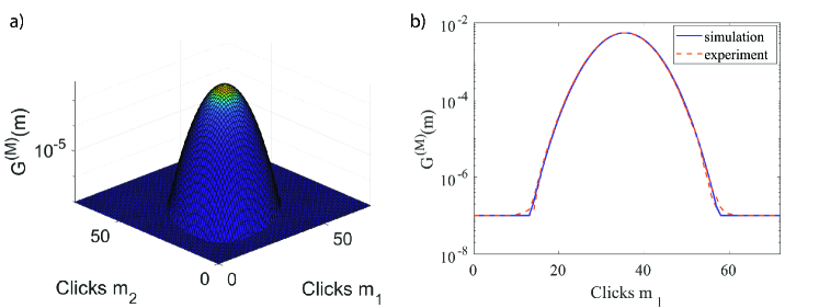
Figure 5: Comparisons of experimental data set $65\mu m$, $1.65W$ with simulations of $1.2\times 10^{6}$ stochastic ensembles for a $d=2$ dimensional GCP, $\mathcal{G}_{72,72}^{(144)}(m_{1},m_{2})$, with input decoherence. a) Full two-dimensional comparison distribution of GCPs with all $73^{2}$ data points. b) One-dimensional slice through the maximum of the two-dimensional distribution. Plots a comparison of grouped count $m_{1}$ where the solid blue line is the theoretical prediction and the orange dashed line is the experimental data.

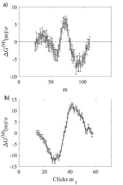
Figure 6: Normalized difference of experiment versus simulation for data set $65\mu m$, $1.65W$ with added decoherence. a) Plots results of $\Delta\mathcal{G}^{(M)}(m)/\sigma_{m}$ versus $m$ for total count probability distributions. b) Results are $\Delta\mathcal{G}^{(M)}(m)/\sigma_{m}$ versus $m_{1}$ of the one-dimensional slice shown in Fig.(5).b which is a $d=2$ dimensional GCP comparison. Upper and lower lines correspond to theoretical sampling errors.

Improved agreement is obtained when decoherence is added to simulations as shown in Table. 1, which contains chi-square and Z-statistic outputs for each data set, with $ET$ denoting the distance between experiment and thermalized distributions. Corresponding fitting parameters are also given.

After input decoherence corresponding to $\approx 2\%$ mode mismatches is included, the samples obtained from an experiment using laser waist and power $65\mu m$, $0.15W$ are closer to the simulated distribution than any other data set, as indicated by the result that $Z\approx 0.7$. Unlike the pure squeezed state comparisons, the Z-statistic shows that detected total count distributions agree with the expected distribution for input squeezed states with added decoherence.

Such good agreement is not the case with most other data sets, where Z values remain large. This is particularly the case with samples corresponding to $65\mu m$, $1.65W$, which required the largest amount of input decoherence, equating to $\approx 4\%$ mode mismatch, to obtain a three-orders of magnitude improvement in $\chi^{2}/k$ values compared to pure state inputs. Despite this improvement, the Z-statistic shows the probability of obtaining such an output is very small, indicating systematic errors.

V.2 Two-dimensional binning comparisons

Waist	Power	Two-dimensional GCP				Four-dimensional GCP
		$Z_{EI}$	$k$	$Z_{ET}$	$k$	$Z_{ET}$	$k$
$125\mu m$	$1.412W$	$181$	$712$	$145$	$702$	$153$	$28855$
	$0.5W$	$125$	$287$	$115$	$285$	$209$	$6479$
$65\mu m$	$1.65W$	$422$	$1582$	$185$	$1567$	$200$	$98682$
	$1W$	$168$	$1274$	$68$	$1267$	$109$	$70826$
	$0.6W$	$107$	$825$	$32$	$815$	$66$	$33271$
	$0.3W$	$105$	$449$	$43$	$445$	$99$	$13605$
	$0.15W$	$76$	$242$	$40$	$240$	$111$	$4695$

Table 2: Summary of Z-statistic test outputs for comparisons of GCPs with dimensions $d=2$ and $d=4$ for all GBS experimental data sets obtained from Ref.[18]. Simulations are performed with $E_{S}=1.2\times 10^{6}$ ensembles for pure squeezed states and thermalized squeezed states with the fitting parameters used to obtain the minimized total counts $\chi^{2}/k$ outputs for each data set obtained from Table. 1.

To gain further insight into the experimental data, we present comparisons of multi-dimensional GCPs with fitting parameters corresponding to those given in Table. 1 for experimental samples of every tested laser waist and power. Due to the large number of valid bins, the Z-statistic is the most useful statistical test for multi-dimensional GCPs. The increased number of data points produces Gaussian distributions with much smaller variances, meaning comparisons are required to pass a more stringent test. Therefore, Z-statistic outputs for multi-dimensional GCPs are presented in Table. 2.

We start by analyzing comparisons of a $d=2$ dimensional GCP, an example of which is plotted in Fig.(5). Output Z values increase for all data sets when compared to the corresponding total count outputs of Table. 1. This is particularly noticeable for data from $65\mu m$, $0.15W$, which sees a forty-fold increase in the $Z$ value, with $Z_{ET}\approx 40$, when compared to total counts for simulations with added decoherence, which have $Z_{ET}\approx 0.7$.

Comparisons with simulations using pure squeezed state inputs record even larger statistical errors, with data from $65\mu m$, $1.65W$ giving $Z_{EI}\approx 422$ for $1582$ valid bins containing more than $10$ counts. This is improved upon by adding decoherence in the inputs, giving $Z_{ET}\approx 185$, which is still very large.

Therefore, statistical testing indicates that experimental samples for all laser waists and powers are further away from the expected multi-dimensional results than comparisons of total counts.

This increased difference between theory and experiment for growing dimension is reflected in Fig.(6), which plots the normalized difference between theory and experiment [23]:

$$\frac{\Delta\mathcal{G}^{(M)}(m)}{\sigma_{m}}=\frac{\bar{\mathcal{G}}-\mathcal{G}^{e}}{\sigma_{m}}.$$ (40)

We use the shorthand notation $\bar{\mathcal{G}}$ to denote the phase-space simulated GCP ensemble mean and $\mathcal{G}^{e}$ to denote the experimental GCP. The normalized difference follows from Eq.(55), except $\sigma_{m}$ only sums over theoretical and experimental variances of the compared $m$ grouped counts.

The finer comparison obtained from increased dimensional GCPs shows experimental data has further, underlying differences that arise when higher-order correlations are simulated. To confirm this is the case, we can repeat the two-dimensional GCP comparison tests an exponential number of times by randomly permuting each binary pattern. Although not all of these tests can be performed, we randomly permute patterns from $65\mu m$, $1.65W$ ten times and $125\mu m$, $1.412W$ five times to determine whether differences remain significant.

Since each random permutation obtains a different value for the grouped count $m_{j}$, comparison differences are likely to vary, with some tests showing better agreement than others. This is seen in Fig.(7) which compares the normalized difference of two random permutations, out of a tested ten, for samples from $65\mu m$, $1.65W$. Although the average Z value for all ten random permutations is $\left\langle Z_{ET}\right\rangle_{rp}\approx 115$ for $\left\langle k\right\rangle_{rp}=1568$, where $\left\langle\dots\right\rangle_{rp}$ denotes averages over random permutations, these two permutations obtain $Z_{ET}\approx 53$ with $k=1547$ and $Z_{ET}\approx 143$ for $1567$ valid bins. Meanwhile five permutations of patterns from $125\mu m$, $1.412W$ output an average of $\left\langle Z_{ET}\right\rangle_{rp}\approx 94$ for $\left\langle k\right\rangle_{rp}=704$.

Each random permutation performed on both data sets generates a mean decrease in $Z$ test outputs when compared to non-permutation comparisons presented in Table. 2. However, every permutation is producing statistical outputs with exponentially small probabilities of being observed.

Therefore, sample detector counts show likely departures from randomness for not only these data sets, but possibly all data sets from this experiment, when compared to both ideal and mode mismatched theoretical distributions.

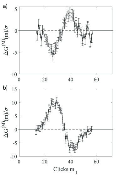
Figure 7: Comparison of normalized differences for two random permutations of binary patterns from data set $65\mu m$, $1.65W$. The observable is a $d=2$ dimensional GCP with input decoherence which is simulated with $E_{S}=1.2\times 10^{6}$. Graphed results are of $\Delta\mathcal{G}^{(M)}(m)/\sigma_{m}$ versus $m_{1}$. a) Plots a random permutation test with a statistic test output of $Z_{ET}\approx 53$ with $k=1547$ valid bins, whilst b) plots a random permutation test with $Z_{ET}\approx 142$ for $k=1567$. Upper and lower lines are $\pm 1\sigma_{T,i}$ theoretical sampling errors.

V.3 Four-dimensional binning comparisons

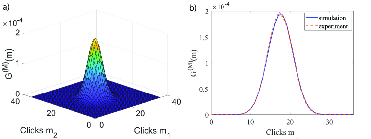
Figure 8: Comparisons of a $d=4$ dimensional GCP, $\mathcal{G}_{36,36,36,36}^{(144)}(m_{1},m_{2},m_{3},m_{4})$, for data set $65\mu m$, $1.65W$ containing $N_{E}=4\times 10^{7}$ experimental binary patterns and phase-space simulations with $E_{S}=1.2\times 10^{6}$ and added decoherence. a) A two-dimensional planar slice of grouped counts $m_{1},m_{2}$ of a four-dimensional distribution. All $37^{4}$ data points are used for statistical tests. b) One-dimensional slice through the maximum of the two-dimensional planar slice. Plot is a comparison of $m_{1}$, where the solid blue line is the theoretical prediction and the orange dashed line is the experimental GCP.

To further test if the experimental data agrees with the Gaussian model, we increased the dimension of the binning to $d=4$. Statistical testing of outputs from each data set are given in Table. 2 and graphical comparisons of samples from $65\mu m$, $1.65W$ are shown in Fig.(8). This relatively moderate increase in dimension causes a dramatic increase in the number of bins satisfying $m_{j}>10$, giving more data points to test.

At first glance, it appears as though the Z-statistic for some data has stabilized, particularly $65\mu m$, $1.65W$ and $125\mu m$, $1.412W$, where the large increases seen when going from one to two-dimensions is not observed. This is further verified by performing comparisons for five random permutations of both data sets, giving averages of $\left\langle Z_{ET}\right\rangle_{rp}\approx 159$ for $\left\langle k\right\rangle_{rp}=99650$ and $\left\langle Z_{ET}\right\rangle_{rp}\approx 136$ for $\left\langle k\right\rangle_{rp}=29175$, respectively.

However, the chi-square and $Z$-statistic tests require summing over both experimental and theoretical sampling errors (see Appendices). Therefore, if either the mean theoretical, $\bar{\sigma}_{T}$, or experimental, $\bar{\sigma}_{E}$, sampling errors satisfy $\bar{\sigma}_{E}\gg\bar{\sigma}_{T}$ or $\bar{\sigma}_{T}\gg\bar{\sigma}_{E}$ while $\bar{\sigma}_{E},\bar{\sigma}_{T}\approx\bar{\Delta}$, where $\bar{\Delta}=\sum_{i}^{k}(\bar{\mathcal{G}}_{i}-\mathcal{G}_{i}^{e})/k$ is the mean difference error, an artificially small $\chi^{2}/k$ is generated causing the $Z$ value to appear to stabilize.

A closer inspection shows experimental sampling errors for non-permutation comparisons of $65\mu m$, $1.65W$ have a mean value of $\bar{\sigma}_{E}\approx 3.6\times 10^{-7}$. This is not only much larger than theoretical sampling errors, $\bar{\sigma}_{T}\approx 2.1\times 10^{-8}$, but also reaches the level where $\bar{\sigma}_{E}\approx\bar{\Delta}$. This is also observed in sampling errors from $125\mu m$, $1.412W$ which satisfy $\bar{\sigma}_{E}\gg\bar{\sigma}_{T}$ for non-permutation comparisons, with $\bar{\sigma}_{E}\approx 5.4\times 10^{-7}$ and $\bar{\sigma}_{T}\approx 4.9\times 10^{-8}$.

The cause of this increase in $\bar{\sigma}_{E}$ is due to experimental GCPs containing many bins with few photon counts per bin. Therefore, with currently available experimental data, experimental sampling errors become significant at four-dimensions, rendering comparisons less accurate.

In other words, there is a balance required between test complexity and sample numbers. While more complex tests are much harder to fake because there are exponentially many of them, there is a price to pay. The amount of experimental data required to give low experimental sampling errors becomes unfeasibly large, reducing the power of the tests. Despite this limitation, we note that for the four-dimensional binning case, $Z_{ET}$ is still too large.

This may indicate that the transmission errors change from mode to mode, which we do not take into account here.

V.4 Low-order moments

Waist	Power	$Z_{EI}$	$Z_{ET}$
$125\mu m$	$1.412W$	$285$	$284$
	$0.5W$	$418$	$425$
$65\mu m$	$1.65W$	$541$	$516$
	$1W$	$405$	$397$
	$0.6W$	$267$	$263$
	$0.3W$	$235$	$231$
	$0.15W$	$198$	$196$

Table 3: Tabulated Z-statistic outputs for all $144$ possible first-order click correlation moments of each data set. Simulations are performed using $1.44\times 10^{7}$ ensembles for input stochastic samples corresponding to pure squeezed states with $\epsilon=0$ and $t=1$, corresponding to the ideal GBS. The distance between experimental data and the simulated ideal output denoted by the subscript $EI$, whilst $ET$ is the distance between experiment and simulations with small admixtures of thermal decoherence corresponding to mode mismatches. Fitting parameters applied to each data set can be found in Table. 1.

Previously, click correlation moments, in the form of cumulants, have been used to verify the presence of non-trivial correlations in experimental data and to determine the accuracy of spoofing algorithms [18, 34]. Comparisons of these marginal distributions are useful in determining whether specific experimental correlations agree with theoretical probabilities.

The simplest of these is the first-order moment, $\left\langle\hat{\pi}_{j}(1)\right\rangle$, for which statistical test results for all experimentally tested laser waists and powers are presented in Table. 3. In contrast to the comparisons presented above for total counts and multi-dimensional GCPs, added decoherence does little to improve statistical test outputs, with all data sets deviating significantly from theory.

Figure 9 plots the first-order click correlation for $65\mu m$, $1.65W$ where simulations contains a small admixture of thermal decoherence. Although comparison plots appear visually matching, graphed normalized differences tell a different story (see Fig. (9).b). This is reflected in statistical testing, where $Z_{ET}\approx 516$ and $Z_{EI}\approx 541$.

Comparisons of correlation moments of orders $n=2,3$ show these deviations increase with order. We perform statistical tests for all possible combinations of output modes for data from $65\mu m$, $1.65W$, where the number of possible combinations of output modes follows $\binom{M}{n}=M!/(n!(M-n)!)$. For graphical simplicity, only a small sample of these combinations are plotted in Fig.(10), for $n=2$, and Fig.(11) with $n=3$.

As in the first-order case, although theoretical and experimental distributions may generate visually similar outputs, $Z$-statistic results of $Z_{ET}\approx 4.3\times 10^{3}$ and $Z_{ET}\approx 2.7\times 10^{4}$ for $n=2,3$, respectively show every increase in correlation order sees an, approximately, order of magnitude increase in Z distances that measure the statistical errors.

An increase in statistical comparison errors with correlation order is not surprising, because the quantity of data compared increases with order. In general, large discrepancies may indicate systematic errors, since outputs are far from their expected mean. Similar effects are observed in the higher dimensional grouped counts, above.

These systematic errors could be caused by variations in transmission or detector efficiency that are not accounted for in the measured parameters, which could be included by fitting the output count data by varying the transmission matrix $T$. However, at least $144$ output fitting parameters would be needed, making these comparisons less meaningful.

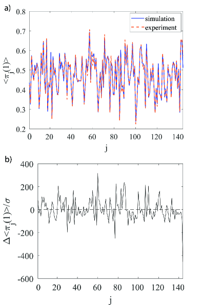
Figure 9: Comparison of theory versus experiment for all possible combinations of first-order count probabilities, $\mathcal{G}_{\{j\}}^{(1)}(1)=\left\langle\hat{\pi}_{j}(1)\right\rangle$, per channel $j$. Experimental samples are obtained from data set $65\mu m$, $1.65W$ whilst simulations are performed using $E_{S}=1.44\times 10^{7}$ ensembles and a small admixture of thermal decoherence. a) Comparison plot with simulations represented by the solid blue and experimental distributions plotted with orange dashed lines. b) Normalized difference of $\Delta\left\langle\hat{\pi}_{j}(1)\right\rangle/\sigma_{m}$ versus $j$.

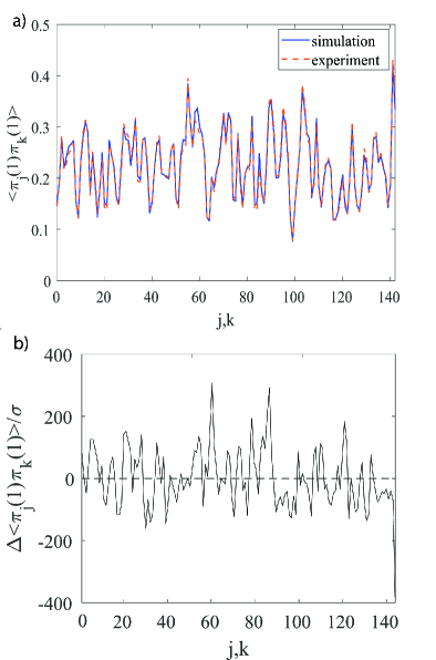
Figure 10: Theoretical and experimental comparison of a small sample of $143$ out of a possible $\binom{144}{2}=10296$ second-order click correlation moments for modes $j,k$. Phase-space simulations use $E_{S}=1.44\times 10^{7}$ ensembles whilst experimental samples are from $65\mu m$, $1.65W$, with input decoherence corresponding to Table. 1. a) Plotted comparisons of $\mathcal{G}_{\{j,k\}}^{(2)}(2)=\left\langle\hat{\pi}_{j}(1)\hat{\pi}_{k}(1)\right\rangle$ versus channels $j,k$ where simulations are represented by the solid blue and experimental outputs are plotted with orange dashed lines. b) Normalized difference of $\Delta\left\langle\hat{\pi}_{j}(1)\hat{\pi}_{k}(1)\right\rangle/\sigma_{m}$ versus $j,k$.

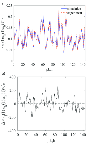
Figure 11: Errors in comparisons of theory and experiment for a subset of $142$ third-order click correlations, $\mathcal{G}_{\{j,k,h\}}^{(3)}(3)=\left\langle\hat{\pi}_{j}(1)\hat{\pi}_{k}(1)\hat{\pi}_{h}(1)\right\rangle$, versus modes $j,k,h$. Statistical tests are performed using all $\binom{144}{3}=487344$ possible combinations of output modes. a) Graphical comparisons with simulations denoted by the solid blue and obtained using $E_{S}=1.44\times 10^{7}$ ensembles with added decoherence in the input stochastic samples, whilst the orange dashed lines denotes experimental outputs from data set $65\mu m$, $1.65W$. b) Normalized difference of $\Delta\left\langle\hat{\pi}_{j}(1)\hat{\pi}_{k}(1)\hat{\pi}_{h}(1)\right\rangle/\sigma_{m}$ versus $j,k,h$.

V.5 Summary

In summary, experimental data does not agree with the ideal state distributions within sampling error, measured by the Z-statistic. This was found for all comparisons. Agreement is greatly improved if the comparison is made with a thermalized quantum model. There are lower discrepancies in total count data compared to mode-dependent data. This suggests that the GBS model could be further refined with better transmission parameter estimates.

VI Classically generated photon counts

There is no known efficient classical method to generate the random binary counts, if the input is a squeezed quantum state Lund et al. [86], Quesada et al. [33], Quesada and Arrazola [87]. However, classical states input into a linear bosonic network with normally ordered detectors generate an output state which is efficiently simulable using Glauber’s diagonal P-representation [66, 65]. This covers thermal, coherent [36, 56, 64], and the recently proposed squashed states [39, 38].

Although experimental GBS data is poorly modeled by thermal states [17, 18, 34], an analysis of experimental data from 100-mode GBS experiments showed that this experiment was best fitted with a strongly thermalized input [23]. A thermal component of $\epsilon=0.0932\pm 0.0005$ was used to model this experiment, which is approximately double the largest $\epsilon$ value presented in Table 1.

Consistent with this, a classical approximation to squeezed states, called squashed states [39], has been shown to agree with the $100$-mode experimental data at least as well as pure state GBS predictions. This is not surprising, as high thermalization levels produce Gaussian states which are nearly classical.

The simplicity in computing output distributions of classical states can be exploited to efficiently generate the corresponding binary random numbers without the exponential time taken to (classically) generate the ideal GBS distribution. This allows comparisons between counts generated with a classical model and ideal GBS theory.

The number of probability distributions of interest can now be extended, of which we are interested in the following four cases:

(I)

Ideal theoretical GBS squeezed state distributions

(E)

Experimentally measured count distributions from data

(T)

Thermalized, but quantum, best fit distributions

(C)

Classical squashed state count distribution data

Using the notation in the Appendix, there are six relevant probability distances that one can measure. The important ones are shown schematically in Figs (1) and (2). For an ideal GBS experiment, one expects that $Z_{EI}\approx 1$, while $Z_{CI}\gg 1$. This would show that the experiment generates the expected exponentially hard random count distributions, but the efficient classical model is unable to generate the same data within sampling errors.

In real experiments, the inputs behave as though thermalized, possibly from mode mismatch. Even this thermalized input can still have quantum effects, provided one can show that $Z_{ET}\approx 1$, while $Z_{CT}\gg 1$ for at least one of the grouped count measures. To prove quantum advantage in this practical but non-ideal case, one must show that this is true for all possible efficient classical random algorithms.

When compared to experimental data from the $144$-mode network of Ref.[18], low-order correlations were found to be a very similar distance from classical squashed states as the ideal GBS marginal probabilities [39]. However, as explained in Section (V.4), low-order correlations are not an optimal measure of quantum versus classical behavior.

Therefore, using the diagonal P-representation, which is a limit of the generalized P-representation, we greatly extend the previous classical count analysis in several extremely important directions: Firstly, we compare experimental networks with simulated classical output distributions, computing the distance measure $Z_{EC}$ for both low and high-order correlations. This has the advantage of including sampling errors, which weren’t analyzed previously.

Secondly, in order to compute the distance between the classical squashed distribution and the theoretical ideal GBS, corresponding to the distance measure $Z_{CI}$, we generate classically faked random binary patterns. These patterns are generated using squeezing parameters and transmission matrix corresponding to experimental networks $65\mu m,1.65W$ and $65\mu m,0.15W$. Comparisons are also made between the classical fakes and the best-fit thermalized model.

VI.1 Classical Gaussian boson sampling

A classically simulable linear bosonic network is one in which $N\subset M$ classical states are input into a GBS where the input density operator can be defined in terms of the diagonal P-representation as:

$$\hat{\rho}^{(\text{in)}}=\int P(\boldsymbol{\alpha})\left|\boldsymbol{\alpha}\right\rangle\left\langle\boldsymbol{\alpha}\right|\text{d}^{2}\boldsymbol{\alpha}.$$ (41)

The diagonal-P distribution $P(\boldsymbol{\alpha})$ for classical states is obtained from Eq.(11) with $\sigma=0$. As one simple example, input thermal states with variance given by Eq.(5), are defined by the distribution [64, 78]

$$P(\boldsymbol{\alpha})=\prod_{j}\left(\frac{1}{\pi n_{j}}e^{-|\alpha_{j}|^{2}/n_{j}}\right).$$ (42)

Squashed states, with variance Eq.(7), are distributed in phase-space following [38]

$$P(\bm{\alpha})=\prod_{j}\sqrt{\frac{1}{2\pi n_{j}}}e^{-\text{Re}\left(\alpha_{j}\right)^{2}/2n_{j}}\delta\left(\text{Im}\left(\alpha_{j}\right)\right).$$ (43)

Since both inputs are Gaussian, initial coherent amplitudes $\boldsymbol{\alpha},\boldsymbol{\alpha}^{*}$ are sampled efficiently from Eq.(20), where for thermal states one has

$$\alpha_{j}=\sqrt{\frac{n_{j}}{2}}\left(w_{j}+iw_{j+M}\right),$$ (44)

whilst for squashed states

$$\alpha_{j}=\alpha_{j}^{*}=\sqrt{n_{j}}w_{j}.$$ (45)

As outlined in subsection II.6 for nonclassical states, output coherent amplitudes are obtained via the transformation

$$\boldsymbol{\alpha}^{\prime} =\boldsymbol{T}\boldsymbol{\alpha}$$

$$\boldsymbol{\alpha}^{\prime*} =(\boldsymbol{T}\boldsymbol{\alpha})^{*},$$ (46)

since we are now in a classical phase-space, with corresponding output density matrix

$$\hat{\rho}^{(\text{out)}}=\int P(\boldsymbol{\alpha})\left|\boldsymbol{T\alpha}\right\rangle\left\langle\boldsymbol{T\alpha}\right|\text{d}^{2}\boldsymbol{\alpha}.$$ (47)

In order to reproduce simulations performed in Ref. [39], output coherent amplitudes are used to simulate GCPs. Following from Eq.(12) for $\sigma=1$, GCPs, as defined in Eq.(27), are now simulated over a classical phase-space such that

$$\mathcal{G}_{\boldsymbol{S}}^{(n)}\left(\boldsymbol{m}\right)=\int P(\boldsymbol{\alpha})\left[\prod_{j=1}^{d}\left[\sum_{\sum c_{i}=m_{j}}\Pi_{S_{j}}\left(\boldsymbol{c}\right)\right]\right]\text{d}^{2}\bm{\alpha},$$ (48)

Here, $\Pi\left(\bm{c}\right)=\bigotimes_{j=1}^{M}\pi_{j}\left(c_{j}\right)$ is the phase-space observable for a binary pattern $\boldsymbol{c}$, where $\pi_{j}$ has the same form as Eq.(28) except now the output photon number is defined as $n^{\prime}_{j}=|\alpha^{\prime}_{j}|^{2}$.

These are not the only efficient classical algorithms that one could use to generate count data, but here we focus on the squashed state case for the purpose of making definite comparisons.

VI.1.1 Generating classical fake bit patterns

In order to determine whether the experimental networks of Ref.[18] generate samples that are closer to the ideal GBS distribution than a classical fake, as one would expect, we also use the coherent amplitudes $\boldsymbol{\alpha}^{\prime}$, $\boldsymbol{\alpha}^{\prime*}$ to generate fake binary patterns.

This is possible due to classical inputs generating an output distribution that can be sampled efficiently [66, 34]. For example, the first-order sampler of Ref.[34] efficiently generated binary patterns by approximating the output of the bosonic network as a thermal state. Although such samplers didn’t implement phase-space methods, both methods produce similar results.

Although this method can be used for any classical input state, we focus on squashed states, since thermal states have been well tested [17, 18, 34].

Initially, the process follows that outlined above; Stochastic amplitudes for $N\subset M$ squashed inputs are generated using Eq.(45) and are transformed to outputs following Eq.(46). The click probability of the $j$-th detector for each individual stochastic trajectory is now computed as

$$(\pi_{j}(1))^{(k)}=(1-e^{-n^{\prime}_{j}})^{(k)},$$ (49)

where $k\in E_{S}$ is a single trajectory in phase-space.

This is straightforwardly extended to the multi-mode case as

$$\boldsymbol{\pi}^{(k)}=[(\pi_{1}(1))^{(k)},(\pi_{2}(1))^{(k)},\dots,(\pi_{M}(1))^{(k)}],$$ (50)

which is a vector of click probabilities for a single trajectory.

Binary patterns can now be efficiently generated by randomly sampling each bit independently using the Bernoulli distribution, which for the $j$-th mode is defined as

$$P_{j}^{(k)}(c_{j}^{(\text{fake)}})=(p_{j}^{(k)})^{c_{j}^{(\text{fake)}}}(1-p_{j}^{(k)})^{1-c_{j}^{(\text{fake)}}},$$ (51)

where $p_{j}^{(k)}=(\pi_{j}(1))^{(k)}$ is the probability of generating the fake click $c_{j}^{(\text{fake)}}=1$. Therefore, each trajectory outputs the fake count vector

$$(\boldsymbol{c}^{(\text{fake})})^{(k)}=[P_{1}^{(k)},P_{2}^{(k)},\dots,P_{M}^{(k)}].$$ (52)

It is clear that the number of classical fake patterns generated scales as $N_{F}=E_{S}$. For these to be useful for comparisons, they are binned to generated grouped counts $m_{j}^{(\text{fake})}=\sum_{i=1}^{M}c_{i}^{(\text{fake})}$. Following Eq.(34), we define the GCP of the $i$-th fake count bin as

$$\mathcal{G}_{i}^{f}=\frac{m_{j_{i}}^{(\text{fake})}}{N_{F}}.$$ (53)

VI.2 Comparisons of classical GBS and experiment

Analogous to Ref.[39], we begin by comparing phase-space simulated GCPs of squashed state inputs to experimentally binned patterns. Here, the distance between experimental and classical GCPs are denoted by the subscript $EC$ (see Appendix for analytical definitions).

Waist	Power	First-order moment	One-dimensional GCP		Two-dimensional GCP
		$Z_{EC}$	$Z_{EC}$	$k$	$Z_{EC}$	$k$
$125\mu m$	$1.412W$	$318$	$371$	$49$	$616$	$663$
	$0.5W$	$463$	$489$	$27$	$735$	$249$
$65\mu m$	$1.65W$	$536$	$204$	$83$	$394$	$1545$
	$1W$	$397$	$160$	$72$	$266$	$1227$
	$0.6W$	$281$	$233$	$54$	$363$	$782$
	$0.3W$	$267$	$399$	$37$	$634$	$408$
	$0.15W$	$234$	$459$	$24$	$675$	$204$

Table 4: $Z$-statistical test outputs of comparisons of all $144$ first-order correlation moments, one and two-dimensional GCPs for all experimental data sets. Phase-space simulations for squashed state inputs are performed for $E_{S}=1.44\times 10^{7}$ensembles for moment comparisons and $E_{S}=1.2\times 10^{6}$ for GCPs. In all cases, the subscript $EC$ denotes the distance between experimental and classical probabilities. Analogous comparisons with nonclassical inputs are presented in Tables. 1, 2 and 3.

VI.2.1 Low-order correlations

Comparisons of first-order click moments are presented in Table. 4 for every data set. When compared to the distance measures shown in Table. 3 for nonclassical inputs, it is clear that for data set $65\mu m,1.65W$ one has $Z_{EC}\gtrsim Z_{EI}$, as reported previously [39].

Increasing the correlation order to $n=2$ sees $Z$ values follow a similar trend with $Z_{EC}\approx 4.7\times 10^{3}$ compared to nonclassical inputs with $Z_{EI}\approx 4.8\times 10^{3}$ and $Z_{ET}\approx 4.3\times 10^{3}$. Meanwhile, third-order moments output $Z_{EC}\approx 3.1\times 10^{4}$ whilst $Z_{EI}\approx 3.1\times 10^{4}$, $Z_{ET}\approx 2.7\times 10^{4}$ for pure and thermalized squeezed input comparison simulations.

For all other data sets, bar $65\mu m,1W$ where $Z_{EI}\approx Z_{ET}\approx Z_{EC}$, first-order moments generated from nonclassical inputs are closer to the experimental marginals than classical inputs. This isn’t surprising for these data sets, as classical inputs into a linear network will generate classical correlations, which are fundamentally different from quantum correlations. As indicated by the large $Z$-statistic values, one would expect a classical GBS to display further non-random behavior in the click probabilities than an experiment containing true quantum correlations.

VI.2.2 Multi-dimensional binning

Increasing the correlation order to $n=M$ and including all output modes in the subset vector $\boldsymbol{S}$, comparisons of one and two-dimensional GCPs are given in Table. 4.

Z-statistic outputs for all data sets other than $65\mu m,1.65W$ satisfy $Z_{EC}>Z_{EI}$ for both total count and two-dimensional GCPs. Therefore, for these data sets, output distributions of simulated squashed states poorly model experimental distributions, with simulated pure squeezed states giving closer agreement with experiment.

This is not the case for data set $65\mu m,1.65W$, with comparisons outputting $Z_{EC}\approx 204$ and $Z_{EC}\approx 394$ for simulations of one and two-dimensional GCPs, respectively. When compared to simulations of the ideal GBS, we see that $Z_{EI}\gtrsim Z_{EC}$. For both low-order moments and multi-dimensional GCPs, simulated ideal and squashed classical distribution are approximately the same distance to experimentally binned patterns from data set $65\mu m,1.65W$.

Although these results agree with previous comparisons [39], experimental samples are just as poorly modeled by squashed inputs as by the ideal GBS. We emphasize that the best agreement between theory and experiment for all possible data sets arises from nonclassical, partially thermalized squeezed state inputs, which output the lowest $\chi^{2}$ and $Z$-statistic values for all tested GCP dimensions.

VI.3 Comparisons of classical and quantum output distributions

Using the method outlined in subsection VI.1.1, we generate $N_{F}=4\times 10^{7}$ classical binary patterns from $E_{S}=4\times 10^{7}$ initial stochastic samples of input squashed states.

Two sets of classically faked patterns are generated using squeezing parameters and transmission matrix $\boldsymbol{T}$ from data sets $65\mu m,1.65W$ and $65\mu m$, $0.15W$. These patterns are binned following Eq.(53) and compared to the ideal GBS distribution, which is simulated using $E_{S}=1.2\times 10^{6}$ ensembles for total counts and two-dimensional GCPs, whilst marginal probabilities are simulated using $E_{S}=1.44\times 10^{7}$.

Two distance measures are of interest in this section; The distance between faked and ideal GCPs, $Z_{IC}$, and the distance between faked and thermalized GCPs, $Z_{CT}$. The first is the usual measure used to dispute claims of quantum advantage for classical inputs [17, 18, 19, 34], whilst the second allows one to determine whether the more realistic nonclassical thermalized distributions can be faked via classical inputs.

	$65\mu m$, $1.65W$				$65\mu m$, $0.15W$
	$Z_{EI}$	$Z_{ET}$	$Z_{CI}$	$Z_{CT}$	$Z_{EI}$	$Z_{ET}$	$Z_{CI}$	$Z_{CT}$
$\left\langle\hat{\pi}_{j}(1)\right\rangle$	$541$	$516$	$98$	$253$	$198$	$196$	$108$	$137$
$\left\langle\hat{\pi}_{j}(1)\hat{\pi}_{k}(1)\right\rangle$	$4.8\times 10^{3}$	$4.3\times 10^{3}$	$856$	$2.7\times 10^{3}$	$2.2\times 10^{3}$	$2.2\times 10^{3}$	$1.5\times 10^{3}$	$1.4\times 10^{3}$
$\mathcal{G}_{144}^{(144)}(m)$	$221$	$23$	$122$	$198$	$49$	$0.7$	$300$	$290$
$\mathcal{G}_{72,72}^{(144)}(m_{1},m_{2})$	$422$	$185$	$199$	$350$	$76$	$40$	$468$	$453$

Table 5: Summary of $Z$-statistic results for comparisons of squashed state fake binary patterns with simulated pure and thermalized squeezed states. $N_{F}=4\times 10^{7}$ fake patterns are generated and binned with squeezing parameters and transmission matrix $\boldsymbol{T}$ from experimental data sets $65\mu m$, $1.65W$ and $65\mu m$, $0.15W$, while phase-space simulations are performed for $E_{S}=1.2\times 10^{6}$. The important distance measures in this table is the distance between faked GCPs and output distributions of the ideal, $Z_{CI}$, and thermalized, $Z_{CT}$, GBS instances. For ease of reference, comparisons presented throughout the paper of experiment with the ideal, $Z_{EI}$, and thermalized, $Z_{ET}$, distributions are also presented.

VI.3.1 Classically faked marginal probabilities

Since the diagonal P-representation only contains diagonal coherent state amplitudes, classical states sent through a bosonic network will only generate classical correlations and one would expect some degree of non-randomness in the photon counts to occur. This made clearer by comparing $Z$ values, which are presented in Table. 5 for first and second-order correlations. Expectedly, classically faked first and second-order correlation moments are far from the ideal for both tested data sets, with $Z_{CI}\approx 98$ and $Z_{CI}\approx 108$ for patterns generated using $\boldsymbol{r}$ and $\boldsymbol{T}$ from $65\mu m$, $1.65W$ and $65\mu m$, $0.15W$, respectively.

Despite this, when compared to experimental marginals, the classical fakes for both data sets are closer to the ideal marginals than the experiment. This is particularly noticeable for fakes obtained from $65\mu m$, $1.65W$, which sees $Z_{EI}\approx 5.5Z_{CI}$ for all tested correlation orders. A graphical representation is presented in Fig.12, which compares the normalized difference of experimental first-order marginals (Fig.12a)) and squashed fakes (Fig.12b)).

Simulated thermalized squeezed inputs, with fitting parameters presented in Table. 1 for each data set, show that the classical squashed fakes are also closer to the thermalized marginals than the experiment. As with the ideal case, fakes generated using $65\mu m$, $1.65W$ data set parameters are closest to the thermalized first-order marginals, with experiments being $Z_{ET}-Z_{CT}=263\sigma$ further away from the simulated distribution than the squashed fakes.

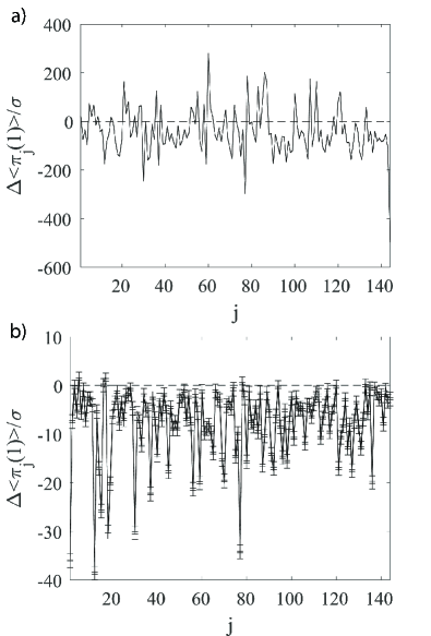
Figure 12: Normalized difference of first-order click correlation moments, $\left\langle\hat{\pi}_{j}(1)\right\rangle$, simulated in phase-space using $E_{S}=1.44\times 10^{7}$ ensembles with pure squeezed state inputs which are compared to a) experimental first-order moments from data set $65\mu m$, $1.65W$ and b) moments generated from classical squashed state faked patterns generated using squeezing parameters and transmission matrix from data set $65\mu m$, $1.65W$.

VI.3.2 Classically faked grouped count probabilities

Although marginal probabilities allow for a direct comparison of specific correlations, they are only part of the picture, and a more thorough analysis is obtained when comparing multi-dimensional GCPs. Since simulations of nonclassical states in phase-space reproduce high-order quantum correlations generated in the network, one expects experimental data to beat classical fakes, which only contain classical correlations.

As outlined in section V, experimental patterns from data set $65\mu m$, $0.15W$ are closer to the pure and thermalized squeezed state output distributions than any other data set. Therefore, we first compare classical squashed fakes generated using squeezing parameters and transmission matrix from this data set to determine whether the thermalized and ideal output distributions can be efficiently faked.

Comparisons of classical fakes with the ideal output for both one and two-dimensional GCPs shows that the classical fake is much further from ideal than the experiment now that higher order correlations are simulated. As seen in Table. 5, Z-statistic tests output $Z_{CI}\approx 300$ and $Z_{CI}\approx 468$ for one and two-dimensional GCPs, whilst experiments output a probability distance of $Z_{EI}\approx 40$ and $Z_{EI}\approx 76$ for the same observables.

Simulations of thermalized squeezed inputs indicate binned faked patterns are even further from the expected distribution, with total counts distances $Z_{CI}\approx 290$ being well over two orders of magnitude larger than the corresponding experimental outputs of $Z\approx 0.7$. Two-dimensional binning show differences with theory on increase for comparisons with classical fakes. Clearly, experimental binary patterns for data set $65\mu m$, $0.15W$ are much closer to both ideal and thermalized distribution once higher-order correlations are considered than their classically faked counterparts.

A different story arises for classical fakes generated using $\boldsymbol{r}$ and $\boldsymbol{T}$ from experimental data set $65\mu m$, $1.65W$. For all GCP dimensions tested, squashed fakes output smaller $Z$ values, and hence smaller $\chi^{2}/k$, for comparisons with simulated pure squeezed state inputs than their experimental counterparts. Apart from using a different classical count generator, this classical advantage was found in a previous investigation of the same dataset Villalonga et al. [34].

Although Z values still indicate a large degree of non-randomness in present in the faked counts, differences are approximately half that of the experiment (see Table. 5) which is made clear in comparisons of total count, where $Z_{EI}\approx 221$ and $Z_{CI}\approx 122$. This can also be seen in Fig. 13 which compares the normalized difference of total counts from experiment and classical fakes.

Increasing the dimension further to $d=4$ sees the $Z$-statistic improve for comparisons with squashed fakes, giving $Z_{CI}\approx 122$. To make comparisons with experimental and fake patterns accurate, we generate an identical number of samples. As described above, experimental sampling errors become significant at $d=4$ due to the large number of bins with too few photons per bin. Therefore, the decrease in Z value of the four-dimensional faked GCP is likely due to an increase in the sampling error as opposed to an improved agreement with theory.

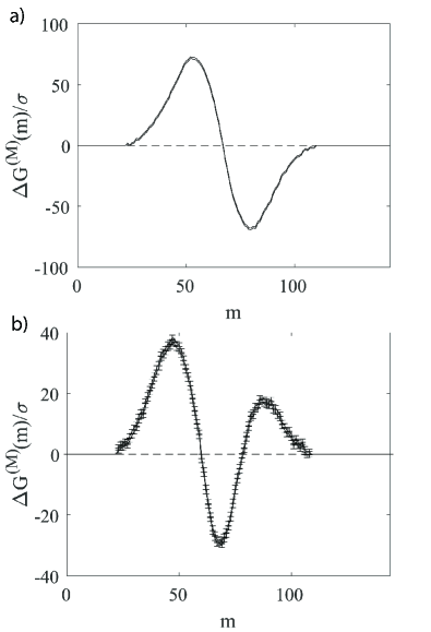
Figure 13: Total count, $\mathcal{G}_{144}^{(144)}(m)$, normalized difference generated from comparisons of simulated pure squeezed states and a) experimental data from $65\mu m$, $1.65W$ and b) fake binary patterns generated using squeezing and transmission matrix from the same data set.

Despite the better agreement between ideal and classical fakes for this data set, distributions corresponding to thermalized squeezed inputs show better agreement with experiment than classical fakes. Total count comparisons Z value of $Z_{ET}\approx 23$ and $Z_{CT}\approx 198$ show significant differences in probability measures, which continue when the dimension is increased to $d=2$, with faked Z values being $165\sigma$ further from the simulated thermalized distribution than the experiment.

Increasing the dimension to $d=4$ further shows that classical fakes poorly replicate thermalized probabilities, with $Z_{ET}\approx 200$ and $Z_{CT}\approx 342$, although both experiment and classical fake $Z$ values indicate photon counts display significant errors once higher order correlations are simulated. This result is expected for classical inputs, but regardless of input state, the current generation of experimental linear networks with saturating detectors, for which computational advantage has been claimed, still show large deviations from theoretical predictions for most of the outputs.

Possible reasons for differences include parameter errors, network fluctuations and nonlinearities. These results highlight the need for a more detailed model of losses and decoherence to fully analyze current linear photonic networks. Despite this, it is encouraging that some low-power total count data gives evidence of computational advantage.

VI.4 Comparison summary

In some cases, classical count simulations performed much better than experimental counts in generating the ideal state distributions. For computational target distributions of a best fit thermalized state, the experiment performs better for the high order correlations. For one low power experiment, we find that the experimental total count distribution also agrees with thermalized theory to within the experimental sampling error, as illustrated in Fig (2).

VII Outlook

Statistical testing of both low and high order correlations is essential for the validation and performance analysis of any large-scale quantum technology. These can detect departures from randomness in experimental photon count data, show the presence of systematic errors and allow one to differentiate experimental data from data spoofed via classical algorithms.

Error-free operation is crucial for any computer, including the present application of linear networks as quantum random number generators [17]. These tests allow one to determine the extent of decoherence present in experiments, which can cause networks to become classically simulable [66], leading to improved designs in future.

Using the efficient positive-P phase-space method introduced in [23], we implement correlation tests of all orders. These include higher dimensional binning algorithms with a randomized test generator, giving a dynamic verification tool that can both validate outputs and potentially prevent faking. We show that, although the current generation of boson sampling quantum computers have outputs that significantly differ from ideal behavior, thermalized yet nonclassical squeezed state inputs generate distributions with the smallest distance to experimental distributions for all data sets tested. However, significant differences persist even when this simple model of modified transmission and partial decoherence is included.

Although errors are larger for inhomogeneous tests like single-channel output counts, this could be caused by estimation errors in the transmission parameters, which are removable with better values. These are less significant than the total count distributions, which are sensitive to a quantum input state. One case with low input powers gave a total count distribution agreeing exactly with the partly thermalized total count distribution.

A strategy of generating “fake” counts from squashed state inputs is also implemented, and shown to have output distributions closer to the ideal than the experiment, for data sets with large laser power. However, at low power, and by extension low numbers of detected counts, the experiment beats the classical squashed fakes, although still with significant errors. Comparisons with a partly thermalized Gaussian model and high order correlations showed that the quantum experiment generated output statistics much closer to this slightly decoherent model than the classical counts.

In summary, there is evidence of computational advantage, but not for the original pure squeezed state input model. Instead, it is for a targeted distribution that is more decoherent than the ideal Gaussian boson sampling input. This is in general agreement with detailed analyses of an earlier experiment [23, 24], where the decoherence was so large that classical models gave similar output statistics [39].

Although these results demonstrate possible computational advantage, they also show that experimental decoherence and other imperfections cause a departure from the ideal model. We therefore suggest that scalable simulators or other methods are essential to the verification and benchmarking of a wide range of large-scale quantum technologies.

Appendix A: Chi-squared tests and sampling errors

The main statistical test used to quantify differences between phase-space simulations of GCPs and experimental outputs is the chi-square test [80]. Chi-square tests are a powerful statistical test commonly used to determine whether observed probabilities obtained from independent samples correspond to the predicted distribution of the system being tested [79, 8].

Let $N_{E}$ denote the number of independent experimental observations. These are classified into $k$ classes denoting all the possible outcomes one can observe. Each class has a theoretical probability of $P_{i}$ with $i=1,2,\dots k$, where the expected number of observations of the $i$-th class is $N_{E}P_{i}$, whilst the actual number of observations from an experiment is $x_{i}$.

The standard chi-square statistic is defined as [8]:

$$\chi^{2}=\sum_{i=1}^{k}\frac{\left(N_{E}P_{i}-x_{i}\right)^{2}}{N_{E}P_{i}},$$ (54)

which can be rewritten in terms of the estimated experimental probability $P_{i}^{e}=x_{i}/N_{E}$ and variance $\sigma_{i}^{2}=P_{i}/N_{E}$.

In terms of GCPs, we define the grouped count of the $i$-th class as $m_{j_{i}}$ with each class representing a detector count bin. Using the shorthand notation $\mathcal{G}_{i}$ to denote the true theoretical GCP of the $i$-th class, the experimental GCP is obtained using $\mathcal{G}_{i}^{e}=m_{j_{i}}/N_{E}$ for $N_{E}$ experimental samples.

Since both experimental and theoretical probabilities are obtained via sampling, a modified version of Eq.(54) is required [23]:

$$\chi^{2}=\sum_{i=1}^{k}\frac{\left(\bar{\mathcal{G}}_{i}-\mathcal{G}_{i}^{e}\right)^{2}}{\sigma_{i}^{2}},$$ (55)

where $\mathcal{\bar{G}}_{i}$ is the phase-space simulated ensemble mean with $\mathcal{G}_{i}=\lim_{E_{S}\rightarrow\infty}\mathcal{\bar{G}}_{i}$ and we define

$$\sigma_{i}^{2}=\sigma_{T,i}^{2}+\sigma_{E,i}^{2}$$ (56)

as the sum of theoretical and experimental sampling errors. This ensures that both the distribution variances are included. For an ideal case, this combination is the theoretical variance of the difference between probabilities $\Delta_{i}=\bar{\mathcal{G}}_{i}-\mathcal{G}_{i}^{e}$, which is called the difference error.

Due to Poissonian fluctuations, experimental sampling errors are estimated as $\sigma_{E,i}\approx\sqrt{\mathcal{G}_{i}/N_{E}}$. These comparisons include both experimental and theoretical variances for best accuracy.

Although the output errors follow a chi-square distribution, the input probabilities in the $\chi^{2}$ sum are required to be both Gaussian, or approximately Gaussian as is the usual case, and independent. Small count numbers per bin means the experimental probability of that bin can no longer be approximated as a Gaussian. Therefore, chi-square tests are only performed for $k$ valid bins, which we define as those having $m_{j_{i}}>10$ [79, 8].

Appendix B: Z-statistic tests

Even though comparisons of measured probabilities with theory are essential to validation tests, Z-statistics have not been used previously to analyze GBS data. Here we give a brief account of this method.

For grouped data, with high enough counts per bin, the expected distributions of measured counts are approximately Gaussian as described above. Hence, for probabilities estimated from experimental measurements, output results are expected to satisfy $\chi^{2}/k-1\approx 0$. The exact value of $\chi^{2}/k$ is then an important indicator that experimental distributions have acceptable errors.

We note that since there are some theoretical sampling errors, we include these error-bars as well. However for experimental data currently available it is not difficult to obtain enough theoretical samples such that this is not an important issue.

Because the experimental data, even after binning, has large numbers of different probabilities, one finds that $k\gg 1$. Hence tabulated chi-square distributions for small $k$ are not useful.

When $k\rightarrow\infty$, the chi-square distribution $\chi^{2}\rightarrow\mathcal{N}(\mu,\sigma^{2})$ with mean $\mu=k$ and variance $\sigma^{2}=2k$, via the central limit theorem [88, 89]. This convergence is slow due to the skewness of the chi-square distribution [89]. Fortunately, an accurate and fast convergence is achieved using the Wilson-Hilferty (WH) transformation [88], where the transformed observable $\left(\chi^{2}/k\right)^{1/3}\rightarrow\mathcal{N}(\mu,\sigma^{2})$ for $k\geq 10$ with $\mu=1-\sigma^{2}$ and $\sigma^{2}=2/(9k)$ [88, 89].

If the chi-square distribution can be approximated as a Gaussian, we can then perform the Z-statistic, or Z-score, test which has the general definition $Z=(X-\mu)/\sigma$ [83, 79], where $X$ is the test statistic. The Z-statistic determines how many standard deviations a test statistic is from its normally distributed expected mean.

In terms of the WH transformed chi-square statistic $X=\left(\chi^{2}/k\right)^{1/3}$, we define an approximate Z-statistic as:

$$Z=\frac{\left(\chi^{2}/k\right)^{1/3}-\left(1-2/(9k)\right)}{\sqrt{2/(9k)}}.$$ (57)

The Z-statistic is used to determine the probability of obtaining the observed chi-square output. A result of $Z>6$ indicates the test statistic has an extremely small probability of being observed.

In GBS with saturating detectors, if detector outcomes are random and independent, one would expect $\left\langle\hat{\pi}_{j}(1)\right\rangle\approx\left\langle\hat{\pi}_{j}(0)\right\rangle$. Therefore, the Z-statistic quantifies whether the observed chi-square distribution corresponds to randomly distributed photon counts. If $Z>6$, one can hypothesize that count patterns are displaying non-random behavior. An example of such non-randomness would be experimental probabilities where $\left\langle\hat{\pi}_{j}(1)\right\rangle\gg\left\langle\hat{\pi}_{j}(0)\right\rangle$. Physically, this may correspond to errors occurring either in the network, generation of input states or detectors themselves, e.g. detector dark counts.

However, the power of the Z-statistic becomes clearer when used to test comparisons with random permutations of binary patterns. If each permutation repeatedly produces chi-square outputs satisfying $\chi^{2}/k\gg 1$, then Z-statistic outputs in turn will satisfy $Z>6$. Therefore, the output $\chi^{2}/k$ values would be highly unlikely to be observed once, when compared to the mean of the resulting WH chi-square distribution, let alone multiple times. This result would indicate systematic errors may be present in the tested network causing events with small probabilities to be continuously observed.

Appendix C: Distance measure notation

Comparisons of GCPs for multiple input states, both classical and nonclassical, with experimental and classically faked binary patterns are presented throughout this paper. Statistical tests of these comparisons result in multiple probability distances being compared. Here, we define each distance measure analytically relative to an estimated count GCP and a theoretical GCP.

As outlined above, the theoretical GCP observable is the phase-space ensemble mean

$$\bar{\mathcal{G}}_{i}=\frac{1}{E_{S}}\sum_{k=1}^{E_{S}}(\mathcal{G}_{i,\sigma})^{(k)},$$ (58)

where $k$ denotes a single trajectory in the entire phase-space and $\mathcal{G}_{i,\sigma}$ is the $\sigma$-ordered stochastic GCP.

Two phase-space methods are used to simulate GCPs: The normally ordered positive-P representation, allowing one to simulate pure and thermalized squeezed states, and the diagonal P-representation, which is only valid for classical input states. Ensemble mean GCPs of the $i$-th class for simulations of pure squeezed states, the ideal output distribution, are denoted as $\bar{\mathcal{G}}_{i,I}$, whilst outputs assuming thermalized and classical input states are $\bar{\mathcal{G}}_{i,T}$ and $\bar{\mathcal{G}}_{i,C}$, respectively.

The normalized distance between experimental GCPs estimated from experimental counts, $\mathcal{G}_{i,E}$, and phase-space simulated theoretical GCPs is computed using a chi-square statistical test which, for generality, is now defined as

$$\chi_{ES}^{2}=\sum_{i=1}^{k}\frac{\left(\mathcal{G}_{i,E}-\bar{\mathcal{G}}_{i,S}\right)^{2}}{\sigma_{i}^{2}},$$ (59)

where $\bar{\mathcal{G}}_{i,S}$ is a stochastic ensemble mean for any general input state, $S$, and $\sigma_{i}^{2}$ is the variance estimate. Comparisons with classically generated (ie, fake) counts, $\mathcal{G}_{i,C}$, give

$$\chi_{CS}^{2}=\sum_{i=1}^{k}\frac{\left(\mathcal{G}_{i,C}-\bar{\mathcal{G}}_{i,S}\right)^{2}}{\sigma_{i}^{2}}.$$ (60)

Each chi-square output is used to compute the $Z$-statistic test as defined above. Therefore, $Z_{ES}$ and $Z_{CS}$ are the corresponding $Z$ values for each probability difference measure. When classically generated fake counts are compared with a classical phase-space moment, they ought to agree within sampling error.

This is shown by $Z_{CC}$ values for two simulation tests presented in the table below. Both tests simulate $N=50$ squashed inputs into the $M=144$ mode experimental network. The first test simulates this classical GBS using squeezing parameters and transmission matrix from data set $65\mu m,0.15W$, whilst the second corresponds to $65\mu m,1.65W$. In both cases, the transmission coefficient is $t=1$.

Phase-space simulations for squashed states are compared to the classical count simulations used for comparisons in the main text, which are generated with the same squeezing and transmission matrix as used in the main simulations. In all these test cases, $Z_{CC}\approx 1$, showing that the distribution moments of the two methods agree within sampling error.

	$Z_{CC}^{(0.15W)}$	$Z_{CC}^{(1.65W)}$
$\left\langle\hat{\pi}_{j}(1)\right\rangle$	$0.8\pm 1$	$1.5\pm 1$
$\mathcal{G}_{M}^{(M)}(m)$	$1.2\pm 1$	$1.6\pm 1$
$\mathcal{G}_{\{M/2,M/2\}}^{(M)}(m_{1},m_{2})$	$1\pm 1$	$0.7\pm 1$

Table 6: Comparisons of $Z$-statistic outputs for phase-space simulations of classical GBS and classical counts. The binned $N_{F}=4\times 10^{7}$ “fake” patterns used in these comparisons are the same as those used for $Z_{CI}$ and $Z_{CT}$ comparisons in the main text using squeezing parameters $\boldsymbol{r}$ and $\boldsymbol{T}$-matrix from data sets $65\mu m,0.15W$ and $65\mu m,1.65W$. Phase-space simulations are performed using $E_{S}=1.2\times 10^{6}$ ensembles with squashed state inputs. The superscripts denote the laser power used for the parameters of the test. This shows excellent agreement between the discrete and phase-space simulations.

References

- Aaronson and Arkhipov [2013] S. Aaronson and A. Arkhipov, The Computational Complexity of Linear Optics, Theory of Computing 9, 143 (2013).
- Hamilton et al. [2017] C. S. Hamilton, R. Kruse, L. Sansoni, S. Barkhofen, C. Silberhorn, and I. Jex, Gaussian boson sampling, Phys. Rev. Lett. 119, 170501 (2017).
- Quesada et al. [2018] N. Quesada, J. M. Arrazola, and N. Killoran, Gaussian boson sampling using threshold detectors, Physical Review A 98, 062322 (2018).
- Bouland [2019] A. Bouland, On the complexity and verification of quantum random circuit sampling, Nature Physics 15, 7 (2019).
- Deshpande et al. [2022] A. Deshpande, A. Mehta, T. Vincent, N. Quesada, M. Hinsche, M. Ioannou, L. Madsen, J. Lavoie, H. Qi, J. Eisert, D. Hangleiter, B. Fefferman, and I. Dhand, Quantum computational advantage via high-dimensional Gaussian boson sampling, Sci. Adv. 8, eabi7894 (2022).
- Zlokapa et al. [2023] A. Zlokapa, B. Villalonga, S. Boixo, and D. A. Lidar, Boundaries of quantum supremacy via random circuit sampling, npj Quantum Information 9, 36 (2023).
- Kim et al. [2023] Y. Kim, A. Eddins, S. Anand, K. X. Wei, E. Van Den Berg, S. Rosenblatt, H. Nayfeh, Y. Wu, M. Zaletel, K. Temme, et al., Evidence for the utility of quantum computing before fault tolerance, Nature 618, 500 (2023).
- Knuth [2014] D. E. Knuth, Art of computer programming, volume 2: Seminumerical algorithms (Addison-Wesley Professional, 2014).
- Broome et al. [2013] M. A. Broome, A. Fedrizzi, S. Rahimi-Keshari, J. Dove, S. Aaronson, T. C. Ralph, and A. G. White, Photonic boson sampling in a tunable circuit, Science 339, 794 (2013).
- Crespi et al. [2013] A. Crespi, R. Osellame, R. Ramponi, D. J. Brod, E. F. Galvao, N. Spagnolo, C. Vitelli, E. Maiorino, P. Mataloni, and F. Sciarrino, Integrated multimode interferometers with arbitrary designs for photonic boson sampling, Nature photonics 7, 545 (2013).
- Tillmann et al. [2013] M. Tillmann, B. Dakić, R. Heilmann, S. Nolte, A. Szameit, and P. Walther, Experimental boson sampling, Nature photonics 7, 540 (2013).
- Spring et al. [2013] J. B. Spring, B. J. Metcalf, P. C. Humphreys, W. S. Kolthammer, X.-M. Jin, M. Barbieri, A. Datta, N. Thomas-Peter, N. K. Langford, D. Kundys, J. C. Gates, B. J. Smith, P. G. R. Smith, and I. A. Walmsley, Boson Sampling on a Photonic Chip, Science 339, 798 (2013).
- Spagnolo et al. [2014] N. Spagnolo, C. Vitelli, M. Bentivegna, D. J. Brod, A. Crespi, F. Flamini, S. Giacomini, G. Milani, R. Ramponi, P. Mataloni, et al., Experimental validation of photonic boson sampling, Nature Photonics 8, 615 (2014).
- Crespi et al. [2016] A. Crespi, R. Osellame, R. Ramponi, M. Bentivegna, F. Flamini, N. Spagnolo, N. Viggianiello, L. Innocenti, P. Mataloni, and F. Sciarrino, Suppression law of quantum states in a 3d photonic fast fourier transform chip, Nature communications 7, 1 (2016).
- Wang et al. [2019] H. Wang, J. Qin, X. Ding, M. C. Chen, S. Chen, X. You, Y. M. He, X. Jiang, L. You, Z. Wang, C. Schneider, J. J. Renema, S. Höfling, C.-Y. Lu, and J. W. Pan, Boson sampling with 20 input photons and a 60-mode interferometer in a -dimensional hilbert space, Physical Review Letters 123, 250503 (2019).
- Kruse et al. [2019] R. Kruse, C. S. Hamilton, L. Sansoni, S. Barkhofen, C. Silberhorn, and I. Jex, Detailed study of gaussian boson sampling, Physical Review A 100, 032326 (2019).
- Zhong et al. [2020] H.-S. Zhong, H. Wang, Y.-H. Deng, M.-C. Chen, L.-C. Peng, Y.-H. Luo, J. Qin, D. Wu, X. Ding, Y. Hu, et al., Quantum computational advantage using photons, Science 370, 1460 (2020).
- Zhong et al. [2021] H.-S. Zhong, Y.-H. Deng, J. Qin, H. Wang, M.-C. Chen, L.-C. Peng, Y.-H. Luo, D. Wu, S.-Q. Gong, H. Su, Y. Hu, P. Hu, X.-Y. Yang, W.-J. Zhang, H. Li, Y. Li, X. Jiang, L. Gan, G. Yang, L. You, Z. Wang, L. Li, N.-L. Liu, J. J. Renema, C.-Y. Lu, and J.-W. Pan, Phase-Programmable Gaussian Boson Sampling Using Stimulated Squeezed Light, Phys. Rev. Lett. 127, 180502 (2021).
- Madsen et al. [2022] L. S. Madsen, F. Laudenbach, M. F. Askarani, F. Rortais, T. Vincent, J. F. F. Bulmer, F. M. Miatto, L. Neuhaus, L. G. Helt, M. J. Collins, A. E. Lita, T. Gerrits, S. W. Nam, V. D. Vaidya, M. Menotti, I. Dhand, Z. Vernon, N. Quesada, and J. Lavoie, Quantum computational advantage with a programmable photonic processor, Nature 606, 75 (2022).
- Aaronson [2011] S. Aaronson, A linear-optical proof that the permanent is p-hard, Proceedings of the Royal Society of London A: Mathematical, Physical and Engineering Sciences 467, 3393 (2011).
- Chabaud et al. [2021] U. Chabaud, G. Ferrini, F. Grosshans, and D. Markham, Classical simulation of gaussian quantum circuits with non-gaussian input states, Phys. Rev. Res. 3, 033018 (2021).
- Chabaud and Walschaers [2023] U. Chabaud and M. Walschaers, Resources for bosonic quantum computational advantage, Phys. Rev. Lett. 130, 090602 (2023).
- Drummond et al. [2022] P. D. Drummond, B. Opanchuk, A. Dellios, and M. D. Reid, Simulating complex networks in phase space: Gaussian boson sampling, Phys. Rev. A 105, 012427 (2022).
- Dellios et al. [2022] A. Dellios, P. D. Drummond, B. Opanchuk, R. Y. Teh, and M. D. Reid, Simulating macroscopic quantum correlations in linear networks, Physics Letters A 429, 127911 (2022).
- Shoji et al. [2017] T. Shoji, K. Aihara, and Y. Yamamoto, Quantum model for coherent ising machines: stochastic differential equations with replicator dynamics, Physical Review A 96, 053833 (2017).
- Wang et al. [2013] Z. Wang, A. Marandi, K. Wen, R. L. Byer, and Y. Yamamoto, Coherent ising machine based on degenerate optical parametric oscillators, Physical Review A 88, 063853 (2013).
- Yamamoto et al. [2017] Y. Yamamoto, K. Aihara, T. Leleu, K.-i. Kawarabayashi, S. Kako, M. Fejer, K. Inoue, and H. Takesue, Coherent ising machines—optical neural networks operating at the quantum limit, npj Quantum Information 3, 1 (2017).
- McMahon et al. [2016] P. L. McMahon, A. Marandi, Y. Haribara, R. Hamerly, C. Langrock, S. Tamate, T. Inagaki, H. Takesue, S. Utsunomiya, K. Aihara, R. L. Byer, M. M. Fejer, H. Mabuchi, and Y. Yamamoto, A fully programmable 100-spin coherent ising machine with all-to-all connections, Science 354, 614 (2016).
- Yamamura et al. [2017] A. Yamamura, K. Aihara, and Y. Yamamoto, Quantum model for coherent ising machines: Discrete-time measurement feedback formulation, Physical Review A 96, 053834 (2017).
- Honjo et al. [2021] T. Honjo, T. Sonobe, K. Inaba, T. Inagaki, T. Ikuta, Y. Yamada, T. Kazama, K. Enbutsu, T. Umeki, R. Kasahara, K. ichi Kawarabayashi, and H. Takesue, 100,000-spin coherent ising machine, Science Advances 7, eabh0952 (2021), https://www.science.org/doi/pdf/10.1126/sciadv.abh0952 .
- Yoshikawa et al. [2016] J.-i. Yoshikawa, S. Yokoyama, T. Kaji, C. Sornphiphatphong, Y. Shiozawa, K. Makino, and A. Furusawa, Invited article: Generation of one-million-mode continuous-variable cluster state by unlimited time-domain multiplexing, APL Photonics 1, 060801 (2016).
- Bulmer et al. [2022] J. F. F. Bulmer, B. A. Bell, R. S. Chadwick, A. E. Jones, D. Moise, A. Rigazzi, J. Thorbecke, U.-U. Haus, T. Van Vaerenbergh, R. B. Patel, I. A. Walmsley, and A. Laing, The boundary for quantum advantage in Gaussian boson sampling, Sci. Adv. 8, eabl9236 (2022).
- Quesada et al. [2022] N. Quesada, R. S. Chadwick, B. A. Bell, J. M. Arrazola, T. Vincent, H. Qi, and R. García-Patrón, Quadratic Speed-Up for Simulating Gaussian Boson Sampling, PRX Quantum 3, 010306 (2022).
- Villalonga et al. [2021] B. Villalonga, M. Y. Niu, L. Li, H. Neven, J. C. Platt, V. N. Smelyanskiy, and S. Boixo, Efficient approximation of experimental gaussian boson sampling, arXiv preprint arXiv:2109.11525 (2021).
- Oh et al. [2022] C. Oh, L. Jiang, and B. Fefferman, Spoofing cross entropy measure in boson sampling (2022), arXiv:2210.15021 [quant-ph] .
- Reid and Walls [1986] M. D. Reid and D. F. Walls, Violations of classical inequalities in quantum optics, Phys. Rev. A 34, 1260 (1986).
- Fearn and Collett [1988] H. Fearn and M. Collett, Representations of squeezed states with thermal noise, Journal of Modern Optics 35, 553 (1988).
- Jahangiri et al. [2020] S. Jahangiri, J. M. Arrazola, N. Quesada, and N. Killoran, Point processes with Gaussian boson sampling, Phys. Rev. E 101, 022134 (2020).
- Martínez-Cifuentes et al. [2022] J. Martínez-Cifuentes, K. M. Fonseca-Romero, and N. Quesada, Classical models are a better explanation of the Jiuzhang Gaussian Boson Samplers than their targeted squeezed light models (2022), arXiv:2207.10058 [quant-ph] .
- Drummond and Gardiner [1980a] P. D. Drummond and C. W. Gardiner, Generalised P-representations in quantum optics, J. Phys. A 13, 2353 (1980a).
- Opanchuk et al. [2018] B. Opanchuk, L. Rosales-Zárate, M. D. Reid, and P. D. Drummond, Simulating and assessing boson sampling experiments with phase-space representations, Physical Review A 97, 042304 (2018).
- Schweigler et al. [2017] T. Schweigler, V. Kasper, S. Erne, I. Mazets, B. Rauer, F. Cataldini, T. Langen, T. Gasenzer, J. Berges, and J. Schmiedmayer, Experimental characterization of a quantum many-body system via higher-order correlations, Nature 545, 323 (2017).
- Marino et al. [2022] J. Marino, M. Eckstein, M. S. Foster, and A. M. Rey, Dynamical phase transitions in the collisionless pre-thermal states of isolated quantum systems: theory and experiments, Reports on Progress in Physics 85, 116001 (2022).
- Blume-Kohout et al. [2022] R. Blume-Kohout, M. P. da Silva, E. Nielsen, T. Proctor, K. Rudinger, M. Sarovar, and K. Young, A taxonomy of small markovian errors, PRX Quantum 3, 020335 (2022).
- Takeuchi and Morimae [2018] Y. Takeuchi and T. Morimae, Verification of many-qubit states, Physical Review X 8, 021060 (2018).
- Goldberg et al. [2022] A. Z. Goldberg, A. M. Steinberg, and K. Heshami, Beyond transcoherent states: Field states for effecting optimal coherent rotations on single or multiple qubits, arXiv preprint arXiv:2210.12167 (2022).
- Maruo et al. [2016] D. Maruo, S. Utsunomiya, and Y. Yamamoto, Truncated wigner theory of coherent ising machines based on degenerate optical parametric oscillator network, Physica Scripta 91, 083010 (2016).
- Kiesewetter and Drummond [2022a] S. Kiesewetter and P. D. Drummond, Phase-space simulations of feedback coherent ising machines, Optics Letters 47, 649 (2022a).
- Kiesewetter and Drummond [2022b] S. Kiesewetter and P. D. Drummond, Coherent ising machine with quantum feedback: The total and conditional master equation methods, Phys. Rev. A 106, 022409 (2022b).
- Drummond and Gardiner [1980b] P. D. Drummond and C. W. Gardiner, Generalised p-representations in quantum optics, Journal of Physics A: Mathematical and General 13, 2353 (1980b).
- Wigner [1932] E. Wigner, On the Quantum Correction For Thermodynamic Equilibrium, Phys. Rev. 40, 749 (1932).
- Moyal [1949] J. E. Moyal, Quantum mechanics as a statistical theory, Mathematical Proceedings of the Cambridge Philosophical Society 45, 99 (1949).
- Husimi [1940] K. Husimi, Some formal properties of the density matrix, Proc. Phys. Math. Soc. Jpn. 22, 264 (1940).
- Hangleiter and Eisert [2022] D. Hangleiter and J. Eisert, Computational advantage of quantum random sampling (2022), arXiv:2206.04079 [cond-mat, physics:quant-ph] .
- Yuen [1976] H. P. Yuen, Two-photon coherent states of the radiation field, Physical Review A 13, 2226 (1976).
- Drummond and Ficek [2004] P. D. Drummond and Z. Ficek, eds., Quantum Squeezing (Springer-Verlag, Berlin, Heidelberg, New York, 2004).
- Vahlbruch et al. [2016] H. Vahlbruch, M. Mehmet, K. Danzmann, and R. Schnabel, Detection of 15 db squeezed states of light and their application for the absolute calibration of photoelectric quantum efficiency, Physical Review Letters 117, 110801 (2016).
- Drummond and Hillery [2014] P. D. Drummond and M. Hillery, The quantum theory of nonlinear optics (Cambridge University Press, 2014).
- Perlmutter et al. [1990] S. H. Perlmutter, M. D. Levenson, R. M. Shelby, and M. B. Weissman, Polarization properties of quasielastic light scattering in fused-silica optical fiber, Phys. Rev. B 42, 5294 (1990).
- Drummond and Opanchuk [2020] P. D. Drummond and B. Opanchuk, Initial states for quantum field simulations in phase space, Physical Review Research 2, 033304 (2020).
- Cahill and Glauber [1969] K. E. Cahill and R. J. Glauber, Ordered Expansions in Boson Amplitude Operators, Phys. Rev. 177, 1857 (1969).
- Glauber [1963a] R. J. Glauber, Coherent and Incoherent States of the Radiation Field, Phys. Rev. 131, 2766 (1963a).
- Sudarshan [1963] E. C. G. Sudarshan, Equivalence of Semiclassical and Quantum Mechanical Descriptions of Statistical Light Beams, Phys. Rev. Lett. 10, 277 (1963).
- Walls and Milburn [2008] D. Walls and G. Milburn, Quantum Optics (Springer, 2008).
- Rahimi-Keshari et al. [2016] S. Rahimi-Keshari, T. C. Ralph, and C. M. Caves, Sufficient Conditions for Efficient Classical Simulation of Quantum Optics, Phys. Rev. X 6, 021039 (2016).
- Qi et al. [2020] H. Qi, D. J. Brod, N. Quesada, and R. García-Patrón, Regimes of classical simulability for noisy gaussian boson sampling, Physical review letters 124, 100502 (2020).
- Louisell [1973] W. H. Louisell, Quantum statistical properties of radiation (Wiley, New York, 1973).
- Hillery et al. [1984] M. Hillery, R. F. O’Connell, M. O. Scully, and E. P. Wigner, Distribution functions in physics: Fundamentals, Phys. Rep. 106, 121 (1984).
- Glauber [1963b] R. J. Glauber, The Quantum Theory of Optical Coherence, Phys. Rev. 130, 2529 (1963b).
- Drummond and Chaturvedi [2016] P. D. Drummond and S. Chaturvedi, Quantum simulations in phase-space: from quantum optics to ultra-cold physics, Physica Scripta 91, 073007 (2016).
- Adam et al. [1994] P. Adam, I. Földesi, and J. Janszky, Complete basis set via straight-line coherent-state superpositions, Physical Review A 49, 1281 (1994).
- Tichy et al. [2014] M. C. Tichy, K. Mayer, A. Buchleitner, and K. Mølmer, Stringent and Efficient Assessment of Boson-Sampling Devices, Phys. Rev. Lett. 113, 020502 (2014).
- Mayer et al. [2011] K. Mayer, M. C. Tichy, F. Mintert, T. Konrad, and A. Buchleitner, Counting statistics of many-particle quantum walks, Phys. Rev. A 83, 062307 (2011).
- Walschaers et al. [2016] M. Walschaers et al., Statistical benchmark for bosonsampling, New Journal of Physics 18, 032001 (2016).
- Sperling et al. [2012] J. Sperling, W. Vogel, and G. S. Agarwal, True photocounting statistics of multiple on-off detectors, Phys. Rev. A 85, 023820 (2012).
- Renema [2020a] J. J. Renema, Marginal probabilities in boson samplers with arbitrary input states, arXiv:2012.14917 [quant-ph] (2020a), arXiv:2012.14917 [quant-ph] .
- Renema [2020b] J. J. Renema, Simulability of partially distinguishable superposition and Gaussian boson sampling, Phys. Rev. A 101, 063840 (2020b).
- Gardiner and Zoller [2004] C. Gardiner and P. Zoller, Quantum Noise: A Handbook of Markovian and Non-Markovian Quantum Stochastic Methods with Applications to Quantum Optics, Springer Series in Synergetics (Springer, 2004).
- Rukhin et al. [2010] A. L. Rukhin, J. Soto, J. R. Nechvatal, M. E. Smid, E. B. Barker, S. D. Leigh, M. Levenson, M. Vangel, D. L. Banks, et al., A statistical test suite for random and pseudorandom number generators for cryptographic applications (2010).
- Pearson [1900] K. Pearson, X. on the criterion that a given system of deviations from the probable in the case of a correlated system of variables is such that it can be reasonably supposed to have arisen from random sampling, The London, Edinburgh, and Dublin Philosophical Magazine and Journal of Science 50, 157 (1900).
- Carter et al. [1987] S. J. Carter, P. D. Drummond, M. D. Reid, and R. M. Shelby, Squeezing of quantum solitons, Physical Review Letters 58, 1841 (1987).
- Kloeden and Platen [1992] P. E. Kloeden and E. Platen, Stochastic Differential Equations, in Numerical Solution of Stochastic Differential Equations (Springer Berlin Heidelberg, Berlin, Heidelberg, 1992) pp. 103–160.
- Freund and Wilson [2003] R. J. Freund and W. J. Wilson, Statistical Methods (Elsevier, 2003).
- [84] Raw data of Jiuzhang 2.0 for sharing | Division of Quantum Physics and Quantum Information, https://quantum.ustc.edu.cn/web/en/node/951.
- [85] GitHub - peterddrummond/xqsim: Quantum network simulations in phase space, https://github.com/peterddrummond/xqsim.
- Lund et al. [2014] A. P. Lund, A. Laing, S. Rahimi-Keshari, T. Rudolph, J. L. O’Brien, and T. C. Ralph, Boson sampling from a gaussian state, Phys. Rev. Lett. 113, 100502 (2014).
- Quesada and Arrazola [2020] N. Quesada and J. M. Arrazola, Exact simulation of gaussian boson sampling in polynomial space and exponential time, Physical Review Research 2, 023005 (2020).
- Wilson and Hilferty [1931] E. B. Wilson and M. M. Hilferty, The Distribution of Chi-Square, Proc. Natl. Acad. Sci. U.S.A. 17, 684 (1931).
- Johnson [1970] N. L. Johnson, Continuous Univariate Distributions, Houghton Mifflin Series in Statistics (Houghton Mifflin, Boston, 1970).