Max-Min Off-Policy Actor-Critic Method Focusing on Worst-Case Robustness to Model Misspecification

Abstract

In the field of reinforcement learning, because of the high cost and risk of policy training in the real world, policies are trained in a simulation environment and transffered to the corresponding real-world environment. However, differences in the environments lead to model misspecification. Multiple studies report significant deterioration of policy performance in a real-world environment. In this study, we focus on scenarios involving a simulation environment with uncertainty parameters and the set of their possible values, called the uncertainty parameter set. The aim is to optimize the worst-case performance on the uncertainty parameter set to guarantee the performance in the corresponding real-world environment. To obtain a policy for the optimization, we propose an off-policy actor-critic approach called the Max-Min Twin Delayed Deep Deterministic Policy Gradient algorithm (M2TD3), which solves a max-min optimization problem using a simultaneous gradient ascent descent approach. Experiments in multi-joint dynamics with contact (MuJoCo) environments show that the proposed method exhibited a worst-case performance superior to several baseline approaches. Our implementation is publicly available (https://github.com/akimotolab/M2TD3).

1 Introduction

Applications of deep reinforcement learning (DRL) to control tasks that involving interaction with the real world are limited because of the need for interaction between the agent and the real-world environment [37]. This difficulty arises because of high interaction time, agent maintenance costs, and safety issues during the interaction. Without enough interactions, DRL tends to overfit to specific interaction histories and yields policies with poor generalizability and safety issues [29].

To solve this problem, simulation environments that estimate the characteristics of real-world environments are often employed, which enable enough interactions for effective DRL application. The policy is trained in the simulation environment and then transferred to the real-world environment [45]. Moreover, because fast and general-purpose simulators, such as Open Dynamics Engine [34], Bullet [3] and multi-joint dynamics with contact (MuJoCo  [38]), are available in the field of robotics, the cost of developing a simulation environment can sometimes be significantly lower than that for real-world interactions.

However, because a simulation environment is an estimation of the real-world environment, discrepancies exist between the two [2]. Even if they are entirely similar, discrepancies may still occur, e.g., because of robot degradation over time or weight changes because of part replacements [22]. Studies report significant degradation of policy trained in a simulation environment when transferred to the corresponding real-world environment [8]. The above discrepancies limit the use of simulator environments in practice and, thus, limit the use of DRL.

In this study, to guarantee performance in the corresponding real-world environment, we aim to obtain a policy that maximizes the expected reward under the worst-case scenario in the uncertainty parameter set $\Omega$. We focus on a scenario where (1) a simulator $\mathcal{M}_{\omega}$ is available, (2) the model uncertainty is parameterized by $\omega\in\Omega$, and $\omega$ is configurable in the simulation, and (3) the real-world environment is identified with some $\omega^{*}\in\Omega$, where $\omega^{*}$ is fixed during an episode; however, (4) $\omega^{*}$ is unknown, is not uniquely determined, or changes from episode to episode. The model of uncertainty described in hypotheses (3) and (4) is referred to as the stationary uncertainty model, in contrast to the time-varying uncertainty model where $\omega^{*}$ can vary during an episode [28]. We develop an off-policy deep deterministic actor-critic approach to optimize the worst-case performance, called the Max-Min Twin Delayed Deep Deterministic Policy Gradient Algorithm (M2TD3). By extending the bi-level optimization formulation of the standard actor-critic method [30], we formulate our problem as a tri-level optimization, where the critic network models a value for each tuple of state, action, and uncertainty parameter, and the actor network models the policy of an agent and an estimate of the worst uncertainty parameter value. Based on the existing deep deterministic actor-critic approach [19; 7], we design an algorithm to solve the tri-level optimization problem by implementing several technical components to stabilize the training, including multiple uncertainty parameters, their refreshing strategies, the uncertainty parameter sampler for interaction, and the soft-min policy update. Numerical experiments on 19 MuJoCo tasks reveal the competitive and superior worst-case performance of our proposed approaches compared to those of several baseline approaches.

2 Preliminaries

We consider an episodic Markov Decision Process (MDP) [6] family $\mathcal{M}_{\Omega}=\{\mathcal{M}_{\omega}\}_{\omega\in\Omega}$, where $\mathcal{M}_{\omega}=\langle S,A,p_{\omega},p^{0}_{\omega},r_{\omega},\gamma\rangle$ is the MDP with uncertainty parameter $\omega\in\Omega$. The state space $S$ and the action space $A$ are subsets of real-valued vector spaces. The transition probability density $p_{\omega}:S\times A\times S\to\mathbb{R}$, the initial state probability density $p^{0}_{\omega}:S\to\mathbb{R}$, and the immediate reward $r_{\omega}:S\times A\to\mathbb{R}$ depend on $\omega$. The discount factor is denoted by $\gamma\in(0,1)$.

We focus on an episodic task on $\mathcal{M}_{\Omega}$. Let $\mu_{\theta}:S\to A$ be a deterministic policy parameterized by $\theta\in\Theta$. Given an uncertainty parameter $\omega\in\Omega$, the initial state follows $s_{0}\sim p_{\omega}^{0}$. At each time step $t\geqslant 0$, the agent observes state $s_{t}$, select action $a_{t}=\mu_{\theta}(s_{t})$, interacts with the environment, and observes the next state $s_{t}^{\prime}\sim p_{\omega}(\cdot\mid s_{t},a_{t})$, the immediate reward $r_{t}=r_{\omega}(s_{t},a_{t})$, and the termination flag $h_{t}$. Here, $h_{t}=1$ if $s_{t}^{\prime}$ is a terminal state or a predefined maximal time step for each past episode; otherwise, $h_{t}=0$. If $h_{t}=0$, let $s_{t+1}=s_{t}^{\prime}$; otherwise, the next state is reset by $s_{t+1}\sim p_{\omega}^{0}$. For simplicity, we let $q_{\omega}(s_{t+1}\mid s_{t},a_{t})$ be the probability density of $s_{t+1}$ given $s_{t}$ and $a_{t}$. The discount reward of the trajectory starting from time step $t$ is $R_{t}=\sum_{k\geqslant 0}\gamma^{k}r_{t+k}$.

The action value function $Q^{\mu_{\theta}}(s,a,\omega)$ under $\omega$ is the expectation of $R_{t}$ starting with $s_{t}=s$ and $a_{t}=a$ under $\omega$; that is, $Q^{\mu_{\theta}}(s,a,\omega)=\mathbb{E}[R_{t}\mid s_{t}=s,a_{t}=a,s_{t+k+1}\sim q_{\omega}(\cdot\mid s_{t+k},\mu_{\theta}(s_{t+k}))\ \forall k\geqslant 0]$, where the expectation is taken over $s_{t+k+1}$ for $k\geqslant 0$. Note that we introduce $\omega$ to the argument to explain the $Q$-value dependence on $\omega$; however, this is essentially the same definition as that for the standard action value function $Q^{\mu_{\theta}}(s,a)$. The recursive formula is as follows:

$$Q^{\mu_{\theta}}(s,a,\omega)=r_{\omega}(s,a)+\gamma\mathbb{E}[Q^{\mu_{\theta}}(s^{\prime},\mu_{\theta}(s^{\prime}),\omega)\mid s^{\prime}\sim q_{\omega}(\cdot\mid s,a)]\enspace.$$ (1)

We consider an off-policy reinforcement learning setting, where the agent interacts with $\mathcal{M}_{\omega}$ using a stochastic behavior policy $\beta:S\times A\to\mathbb{R}$. However, the target policy to be optimized, denoted by $\mu_{\theta}$, is deterministic. Under a fixed $\omega\in\Omega$, the standard objective of off-policy learning is to maximize the expected action value function over the stationary distribution $\rho^{\beta}$, such that

$$J_{\omega}(\theta)=\int_{s\in S}\rho^{\beta}(s\mid\omega)Q^{\mu_{\theta}}(s,\mu_{\theta}(s),\omega)\mathrm{d}s\enspace.$$ (2)

Here, $\rho^{\beta}(s\mid\omega)=\lim_{T\to\infty}\frac{1}{T}\sum_{t=0}^{T-1}\int_{s_{0}}q_{\omega,\beta}^{t}(s\mid s_{0})p_{\omega}^{0}(s_{0})\mathrm{d}s_{0}$ denotes the stationary distribution under $\beta$ and a fixed $\omega\in\Omega$, where the step-$t$ transition probability density $q_{\omega,\beta}^{t}$ is defined as $q_{\omega,\beta}^{1}(s^{\prime}\mid s)=\textstyle\int_{a\in A}q_{\omega}(s^{\prime}\mid s,a)\beta(a\mid s)\mathrm{d}a$ and $q_{\omega,\beta}^{t}(s^{\prime}\mid s)=\textstyle\int_{\bar{s}\in S}q_{\omega,\beta}^{t-1}(\bar{s}\mid s)q_{\omega,\beta}^{1}(s^{\prime}\mid\bar{s})\mathrm{d}\bar{s}$.

We assume that the agent can interact with $\mathcal{M}_{\omega}$ for any $\omega\in\Omega$ during the training and can change $\omega$ after every episode, that is, when $h_{t}=1$. Our objective is to obtain the $\mu_{\theta}$ that maximizes $J_{\omega}(\theta)$ under the worst environment $\omega\in\Omega$. Hence, we tackle the max-min optimization problem requiring $\max_{\theta\in\Theta}\min_{\omega\in\Omega}J_{\omega}(\theta)$.

3 M2TD3

We propose an off-policy actor-critic approach to obtain a policy that maximizes the worst-case performance on $\mathcal{M}_{\Omega}$, called M2TD3. Our approach is based on TD3, an off-policy actor-critic algorithm for a deterministic target policy. In TD3, the critic network $Q_{\phi}$ parameterized by $\phi\in\Phi$ is trained to approximate the $Q^{\mu_{\theta}}$ of $\mu_{\theta}$, whereas the actor network models $\mu_{\theta}$ with parameter $\theta\in\Theta$ and is trained to maximize $J_{\omega}(\theta)$. Moreover, $\omega$ is not considered and is fixed during the training. In this study, to obtain the $\mu_{\theta}$ that maximizes the performance under the worst $\omega$, we extend TD3 by formulating the objective as a maximin problem and introducing a simultaneous gradient ascent descent approach.

The main difficulty in the worst-case performance maximization is in estimating the worst-case performance. Because the objective is expected to be non-concave with respect to (w.r.t.) the uncertainty parameter because of deep actor-critic networks, solving this problem is considered intractable in general [4]. To stabilize the worst-case performance estimation, we introduce various techniques: multiple uncertainty parameters, an uncertainty parameter refresh strategy, and an uncertainty parameter sampler.

Formulation

We can formulate our objective as the following tri-level optimization:

$$\max_{\theta\in\Theta}\min_{\hat{\omega}\in\Omega}J(\theta,\hat{\omega};\phi^{*})\quad\text{s.t.}\quad\phi^{*}\in\operatornamewithlimits{argmin}_{\phi\in\Phi}L(\phi;\theta)\enspace,$$ (3)

where $J$ and $L$ are defined below. Note that this tri-level optimization formulation is an extension of the bi-level optimization formulation of the actor-critic approach proposed in [30].

We introduce a probability density $\alpha:\Omega\to\mathbb{R}$, from which an $\omega$ to be used in the interaction during the training phase is drawn for each episode. The relationship between $\hat{\omega}$ and $\alpha$ is similar to that between $\theta$ and $\beta$: namely, $\hat{\omega}$ and $\theta$ are the parameters to be optimized while $\alpha$ and $\beta$ are introduced for exploration. Let $\rho_{\alpha}^{\beta}(s)=\int_{\omega\in\Omega}\rho^{\beta}(s\mid\omega)\alpha(\omega)\mathrm{d}\omega$ and $\rho_{\alpha}^{\beta}(s,a,\omega)=\beta(a\mid s)\rho^{\beta}(s\mid\omega)\alpha(\omega)$ be the stationary distribution of $s$ and the joint stationary distribution of $(s,a,\omega)$, respectively, under $\alpha$ and $\beta$.

The critic loss function $L(\phi;\theta)$ is designed to simulate the Q-learning algorithm. Let $T_{\mu_{\theta}}$ be the function satisfying $T_{\mu_{\theta}}[Q](s,a,\omega)=r_{\omega}(s,a)+\gamma\int_{s^{\prime}\in S}Q(s^{\prime},\mu_{\theta}(s^{\prime}),\omega)q_{\omega}(s^{\prime}\mid s,a)\mathrm{d}s^{\prime}$. Then, (1) states that $Q^{\mu_{\theta}}$ is the solution to $Q=T_{\mu_{\theta}}[Q]$. Therefore, the critic is trained to minimize the difference between $Q_{\phi}$ and $T_{\mu_{\theta}}[Q_{\phi}]$. This is achieved by minimizing

$$L(\phi;\theta):=\int_{s\in S}\int_{a\in A}\int_{\omega\in\Omega}(T_{\mu_{\theta}}[Q_{\phi}](s,a,\omega)-Q_{\phi}(s,a,\omega))^{2}\rho_{\alpha}^{\beta}(s,a,\omega)\mathrm{d}s\mathrm{d}a\mathrm{d}\omega\enspace.$$ (4)

The max-min objective function of the actor network

$$J(\theta,\hat{\omega};\phi) :=\int_{s\in S}Q_{\phi}(s,\mu_{\theta}(s),\hat{\omega})\rho_{\alpha}^{\beta}(s)\mathrm{d}s$$ (5)

measures the performance of $\mu_{\theta}$ under the uncertainty parameter $\hat{\omega}\in\Omega$ approximated using the critic network $Q_{\phi}$ instead of the ground truth $Q^{\mu_{\theta}}$. Similar to the standard actor-critic approach, we expect $Q_{\phi}$ to approach $Q^{\mu_{\theta}}$ as the critic loss is minimized. Therefore, we expect $J(\theta,\hat{\omega};\phi^{*})$ approximates $\int_{s\in S}Q^{\mu_{\theta}}(s,\mu_{\theta}(s),\hat{\omega})\rho_{\alpha}^{\beta}(s)\mathrm{d}s$ once we obtain $\phi^{*}\approx\operatornamewithlimits{argmin}_{\phi\in\Phi}L(\phi;\theta)$.

Particularly, even if $Q_{\phi^{*}}=Q^{\mu_{\theta}}$, our objective function $J(\theta,\hat{\omega};\phi^{*})$ differs from $J_{\omega}(\theta)$ with $\omega=\hat{\omega}$ in (2), in that the stationary distribution $\rho^{\beta}(s\mid\omega)$ under fixed $\omega$ in $J_{\omega}$ is replaced with $\rho_{\alpha}^{\beta}(s)$ under $\omega\sim\alpha$. However, this change allows us to effectively utilize the replay buffer, which stores the interaction history, to approximate the objective $J(\theta,\hat{\omega};\phi)$. Moreover, if $\alpha$ is concentrated at $\hat{\omega}$, $J(\theta,\hat{\omega};\phi^{*})$ coincides with $J_{\omega=\hat{\omega}}(\theta)$.

Algorithmic Framework

The framework of M2TD3 is designed to solve the tri-level optimization (3). The overall framework of M2TD3 follows that of TD3. In each episode, an uncertainty parameter $\omega$ is sampled from $\alpha$. The training agent interacts with the environment $\mathcal{M}_{\omega}$ using behavior policy $\beta$. At each time step $t$, the transition $(s_{t},a_{t},r_{t},s_{t}^{\prime},h_{t},\omega)$ is stored in the replay buffer, which is denoted by $B$. The critic network $Q_{\phi}$ is trained at every time step, to minimize (4), with a mini-batch being drawn uniformly randomly from $B$. The actor network $\mu_{\theta}$ and the worst-case uncertainty parameter $\hat{\omega}$ are trained in every $T_{\text{freq}}$ step to optimize (5). Note that a uniform random sample $(s,a,\omega)$ taken from $B$ can be regarded as a sample from the stationary distribution $\rho_{\alpha}^{\beta}(s,a,\omega)$. Similarly, $s$ taken from $B$ is regarded as a sample from $\rho_{\alpha}^{\beta}(s)$. These facts allow approximation of the expectations in (4) and (5) using the Monte Carlo method with mini-batch samples uniformly randomly taken from $B$. An algorithmic overview of the proposed method is summarized in Algorithm 1. We have underlined the differences from the general off-policy actor-critic method in the episodic settings. A detailed description of M2TD3 is summarized in Algorithm 2 in Appendix A. As shown from Algorithm 1, the differences between the proposed method and the general off-policy actor-critic are as follows: (1) the introduction of an uncertainty parameter sampler, (2) definition and updating method of critic, and (3) updating method of actor and uncertainty parameters.

Algorithm 1 Algorithmic overview of the proposed method

1:  Draw uncertainty parameter $\omega\sim\alpha_{0}$

2:  Observe initial state $s\sim p_{\omega}^{0}$

3:  for $\mathrm{t}=1$ to $T_{\text{max}}$ do

4:     # interaction

5:     Select action $a\sim\beta_{t}(s)$

6:     Interact with $\mathcal{M}_{\omega}$ with $a$, observe next state $s^{\prime}$, immediate reward $r$ and termination flag $h$

7:     Store transition tuple $(s,a,r,s^{\prime},h,\omega)$ in $B$

8:     if $h=1$ then

9:        Reset uncertainty parameter $\omega\sim\alpha_{t}$

10:        Observe initial state $s\sim p_{\omega}^{0}$

11:     else

12:        Update current state $s\leftarrow s^{\prime}$

13:     end if

14:     # learning

15:     Sample mini-batch $\{(s_{i},a_{i},r_{i},s_{i}^{\prime},h_{i},\omega_{i})\}$ of $\mathrm{M}$ transitions uniform-randomly from $B$

16:     Update the critic network by optimizing Equation 6

17:     Update the actor network and the uncertainty parameter by optimizing Equation 7

18:     Update uncertainty parameter sampler $\alpha$

19:  end for

Critic Update

The critic network update, namely, minimization of (4), is performed by implementing the TD error-based approach. The concept is as follows. Let $\{(s_{i},a_{i},r_{i},s_{i}^{\prime},\omega_{i})\}_{i=1}^{M}\subset B$ be the mini-batch, and let $\theta_{t}$ and $\phi_{t}$ be the actor and critic parameters at time step $t$, respectively. For each tuple, $T_{\mu_{\theta_{t}}}[Q_{\phi_{t}}](s_{i},a_{i},\omega_{i})$ is approximated by $y_{i}=r_{i}+\gamma\cdot Q_{\phi_{t}}(s_{i}^{\prime},\mu_{\theta_{t}}(s_{i}^{\prime}),\omega_{i})$. Then, $L(\phi_{t};\theta_{t})$ in (4) is approximated by the mean square error $\tilde{L}(\phi_{t})$, such that

$$\tilde{L}(\phi_{t})=\frac{1}{M}\sum_{i=1}^{M}(y_{i}-Q_{\phi_{t}}(s_{i},a_{i},\omega_{i}))^{2}\enspace.$$ (6)

Then, the update follows $\phi_{t+1}=\phi_{t}-\lambda_{\phi}\nabla_{\phi}\tilde{L}(\phi_{t})$.

We incorporate the techniques introduced in TD3 to stabilize the training: clipped double Q-learning, target policy smoothing regularization, and target networks. Additionally, we introduce the smoothing regularization for the uncertainty parameter so that the critic is smooth w.r.t. $\hat{\omega}$. Algorithm 3 in Appendix A summarizes the critic update and the details of each technique are available in [7].

Actor Update

Updating of the actor as well as the uncertainty parameter, namely, maximin optimization of (5), is performed via simultaneous gradient ascent descent [27], summarized in Algorithm 4 in Appendix A. Let $\phi_{t}$, $\theta_{t}$ and $\hat{\omega}_{t}$ be the critic, policy, and the uncertainty parameters, respectively, at time step $t$. Instead of the optimal $\phi^{*}$ in (3), we use $\phi_{t}$ as its estimate. With the mini-batch $\{s_{i}\}_{i=1}^{M}\subset B$, we approximate the max-min objective (5) follows:

$$\tilde{J}_{t}(\theta,\hat{\omega}) =\frac{1}{M}\sum_{i=1}^{M}Q_{\phi_{t}}(s_{i},\mu_{\theta}(s),\hat{\omega})\enspace.$$ (7)

We update $\theta$ and $\hat{\omega}$ as $\theta_{t+1}=\theta_{t}+\lambda_{\theta}\nabla_{\theta}\tilde{J}_{t}(\theta_{t},\hat{\omega}_{t})$ and $\hat{\omega}_{t+1}=\hat{\omega}_{t}-\lambda_{\omega}\nabla_{\hat{\omega}}\tilde{J}_{t}(\theta_{t},\hat{\omega}_{t})$, respectively.

For higher-stability performance, we introduce multiple uncertainty parameters. The motivation is twofold. One is to deal with multiple local minima of $J_{t}(\theta,\hat{\omega};\phi^{*})$ w.r.t. $\hat{\omega}$. As the critic network becomes generally non-convex, there may exist multiple local minima of $J_{t}(\theta,\hat{\omega};\phi^{*})$ w.r.t. $\hat{\omega}$. Once $\hat{\omega}$ is stacked at a local minimum point, e.g., $\hat{\omega}^{*}$, $\theta$ may be trained to be robust around a neighborhood of $\hat{\omega}^{*}$ and to perform poorly outside that neighborhood. The other is that the maximin solution $(\theta^{*},\phi^{*})$ of $J_{t}(\theta,\hat{\omega};\phi^{*})$ is not a saddle point, which occurs when the objective is non-concave in $\hat{\omega}$ [14]. Here, more than one $\hat{\omega}$ is necessary to approximate the worst-case performance $\min_{\hat{\omega}}J_{t}(\theta,\hat{\omega};\phi^{*})$ around $(\theta^{*},\phi^{*})$ and a standard simultaneous gradient ascent descent method fails to converge. To relax this defect of simultaneous gradient ascent descent methods, we maintain multiple candidates for the worst $\hat{\omega}$, denoted by $\hat{\omega}_{1},\dots,\hat{\omega}_{N}$. Therefore, replacing $\min_{\hat{\omega}}J(\theta,\hat{\omega};\phi^{*})$ with $\min_{k=1,\dots,N}J(\theta,\hat{\omega}_{k};\phi^{*})$ in (5) has no effect on the optimal $\theta$; however, this change does affect the training behavior. Our update follows the simultaneous gradient ascent descent on $\min_{k=1,\dots,N}J_{t}(\theta,\hat{\omega}_{k})$: $\theta\leftarrow\theta+\lambda_{\theta}\nabla_{\theta}(\min_{k=1,\dots,N}J_{t}(\theta,\hat{\omega}_{k}))$ and $\hat{\omega}_{k}\leftarrow\hat{\omega}_{k}-\lambda_{\omega}\nabla_{\hat{\omega}_{k}}(\min_{\ell=1,\dots,N}J_{t}(\theta,\hat{\omega}_{\ell}))$ for $k=1,\dots,N$. Hence, $\theta$ is updated against the worst $\hat{\omega}_{k}$, and only the worst $\hat{\omega}_{k}$ is updated because the gradient w.r.t. the other $\hat{\omega}_{k}$ is zero.

For multiple uncertainty parameters to be effective, they must be distant from each other. Moreover, all are expected to be selected as the worst parameters with non-negligible frequencies. Otherwise, the advantage of having multiple uncertainty parameters is lessened. From this perspective, we introduce a refreshing strategy for uncertainty parameters. Namely, we resample $\hat{\omega}_{k}\sim\mathcal{U}(\Omega)$ if one of the following scenarios is observed: there exists $\hat{\omega}_{\ell}$ such that the distance $d_{\hat{\omega}}(\hat{\omega}_{k},\hat{\omega}_{\ell})\leqslant d_{\mathrm{thre}}$; the frequency $p_{k}$ of $\hat{\omega}_{k}$ being selected as the worst-case during the actor update is no greater than $p_{\mathrm{thre}}$.

Uncertainty Parameter Sampler

The uncertainty parameter sampler $\alpha$ controls the exploration-exploitation trade-off in the uncertainty parameter. Exploration in $\Omega$ is necessary to train the critic network. If the critic network is not well trained over $\Omega$, it is difficult to locate the worst $\hat{\omega}$ correctly. On the other hand, for $J(\theta,\hat{\omega};\phi^{*})$ in (5) to coincide with $J_{\omega}(\theta)$ for $\omega=\hat{\omega}$ in (2), we require $\alpha$ to be concentrated at $\hat{\omega}$. Otherwise, the optimal $\theta$ for $J(\theta,\hat{\omega};\phi^{*})$ may deviate from that of $J_{\omega}(\theta)$. We design $\alpha$ as follows. For the first $T_{\text{rand}}$ steps, we sample the uncertainty parameter $\omega$ uniformly randomly on $\Omega$, i.e., $\alpha=\mathcal{U}(\Omega)$. Then, we set $\alpha=\sum_{k=1}^{N}p_{k}\cdot\mathcal{N}(\hat{\omega}_{k},\Sigma_{\omega})$, where $\Sigma_{\omega}$ is the predefined covariance matrix. We decrease $\Sigma_{\omega}$ as the time step increases. The rationale behind the gradual decrease of $\Sigma_{\omega}$ is that the training of the critic network is still important after $T_{\text{rand}}$ to make the estimation of the worst-case uncertainty parameter accurate. Details are provided in Appendix C.

4 Related Work

Methods to handle model misspecification include (1) robust policy searching [26; 31; 23; 17; 12; 22], (2) transfer learning [36; 43; 32], (3) domain randomization (DR) [37], and (4) approaches minimizing worst-case sub-optimality gap [5; 21]. Robust policy searching includes methods that aim to obtain the optimal policy under the worst possible disturbance or model misspecification, i.e., maximization of $\min_{\omega\in\Omega}J_{\omega}(\theta)$ for an explicitly or implicitly defined $\Omega$. Transfer learning is a method in which a policy is trained on source tasks and then fine-tuned through interactions while performing the target task. DR is a method in which a policy is trained on source tasks that are sampled randomly from $\mathcal{M}_{\Omega}$. There are two types of DR approaches: vanilla and guided. In vanilla DR [37], the policy is trained on source tasks that are randomly sampled from a pre-defined distribution on $\Omega$. In guided DR [44], the policy is trained on source tasks; however, the $\omega$ distribution is guided towards the target task. Because we do not assume access to the target task, transfer learning and many guided DR approaches are outside the scope of this work. Some guided DR approaches, such as active domain randomization [24], do not access the target task or consider worst-case optimization either. Vanilla DR can be applied to the setting considered here. However, the objective of vanilla DR differs from the present aim, i.e., to maximize the performance averaged over $\Omega$, namely, $\mathbb{E}_{\omega}[J_{\omega}(\theta)\mid\omega\sim\mathcal{U}(\Omega)]$, if the sampling distribution is $\mathcal{U}(\Omega)$. The approaches minimizing the worst-case sub-optimality gap [5; 21] do not optimize the worst-case performance, instead attempt to obtain a policy that generalizes well on the uncertainty parameter set while avoiding too conservative performance, which often attributes to the worst-case performance optimization.

Some robust policy search methods, some adopt an adversarial approach to policy optimization. For example, Robust Adversarial Reinforcement Learning (RARL) [31] models the disturbance caused by an external force produced by an adversarial agent, and alternatively trains the protagonist and adversarial agents. Robust Reinforcement Learning (RRL) [26] similarly models the disturbance but has not been applied to the DRL framework. Minimax Multi-Agent Deep Deterministic Policy Gradient (M3DDPG) [17] has been designed to obtain a robust policy for multi-agent settings. This method is applicable to the setting targeted in this study if only two agents are considered. The above approaches frame the problem as a zero-sum game between a protagonist agent attempting to optimize $\mu_{\theta}$ and an adversarial agent attempting to minimize the protagonist’s performance, hindering the protagonist by generating the worst possible disturbance. Adv-Soft Actor Critic (Adv-SAC) [13] learns policies that are robust to both internal disturbances in the robot’s joint space and those from other robots. Recurrent SAC (RSAC) [42] introduces POMDPs to treat the uncertainty parameter as an unobservable state. A DDPG based approach robustified by applying stochastic gradient langevin dynamics is proposed under the noisy robust MDP setting [15]. However, it has been reported in [42; 15] that their worst-case performances are sometimes even worse than their baseline non-robust approaches. State-Adversarial-DRL (SA-DRL) [48], and alternating training with learned adversaries (ATLA) [47] improve the robustness of DRL agents by using an adversary that perturbs the observations in SAMDP framework that characterizes the decision-making problem in an adversarial attack on state observations. They do not address the model misspecification in the reward and transition functions.

Other approaches attempt to estimate the robust value function, i.e., a value function under the worst uncertainty parameter. Among them, Robust Dynamic Programming (DP) [12] is a DP approach, while the Robust Options Policy Iteration (ROPI) [23] incorporates robustness into option learning [35], which allows agents to learn both hierarchical policies and their corresponding option sets. ROPI is a type of Robust MDP approach [39; 20]. Robust Maximum A-posteriori Policy Optimization (R-MPO) [22] incorporates robustness in MPO [1].

Neither Robust MDP nor R-MPO require interaction with $M_{\omega}$ for an arbitrary $\omega\in\Omega$. This can be advantageous in scenarios where the design of a simulator valid over $\Omega$ is tedious. However, these methods typically require additional assumptions for computating the worst-case for each value function update, such as the finiteness of the state-action space and/or the finiteness of $\Omega$. To apply R-MPO to our setting, finite scenarios from $\Omega$ for training are sampled, but the choice of the training scenarios affects the worst-case performance.

Additionally, to optimize the worst-case performance in the field of offline RL [40; 46; 41], offline RL attempts to obtain robust measures by introducing the principle of pessimism. Some studies that introduce the principle of pessimism in the model-free context [40; 41] and in the actor-critic context [46]. However, these do not compete with this study due to differences in motivation and because offline RL requires additional assumptions in the datasets [46; 41] and realizability [40].

Table 5 in Appendix D summarizes the robust policy search method taxonomy. Our proposed approach, M2TD3, considers the uncertainties in both the reward function and transition probability. The state and action spaces, as well as the uncertainty set, are assumed to be continuous. Table 6 in Appendix D compares the related methods considering their action value function definitions. Methods that do not explicitly utilize the action value function are interpreted from the objective functions. Both M3DDPG and M2TD3 maintain the value function for the tuple of $(s,a,\omega)$. However, M3DDPG takes the worst $\omega^{\prime}$ on the right-hand side, yielding a more conservative policy than M2TD3 for our setting because we assume a stationary uncertainty model, whereas M3DDPG assumes a time-varying uncertainty model in nature [28]. The value functions in RARL and M2TD3 are identical if $\omega$ is fixed. Particularly, $\omega$ is not introduced to the RARL value function because it does not simultaneously optimize $\mu_{\theta}$ and the estimate of the worst $\omega$. RARL repeats the $\theta$ and $\hat{\omega}$ optimizations alternatively. In contrast, M2TD3 optimizes $\theta$ and $\hat{\omega}$ simultaneously in a manner similar to the training processes of generative adversarial networks (GANs) [9]. Hence, we require an action value for each $\omega\in\Omega$.

A difference exists between the optimization strategies of RARL and M2TD3. As noted in the aforementioned section, both methods attempt to maximize the worst-case performance $\min_{\omega\in\Omega}J_{\omega}(\theta)$. Conceptually, RARL repeats $\theta\leftarrow\operatornamewithlimits{argmax}_{\theta}J_{\omega}(\theta)$ and $\omega\leftarrow\operatornamewithlimits{argmin}_{\omega}J_{\omega}(\theta)$. However, this optimization strategy fails to converge even if the objective function $(\theta,\omega)\mapsto J_{\omega}(\theta)$ is concave-convex. As an example, consider the function $(x,y)\mapsto y^{2}-x^{2}+\alpha xy$. The RARL optimization strategy reads $x\leftarrow(\alpha/2)y$ and $y\leftarrow-(\alpha/2)x$, which causes divergence if $\alpha>2$. Alternating updates are also employed in other approaches such as Adv-SAC, SA-DRL, and ATLA. These share the same potential issue as RARL. M2TD3 attempts to alleviate this divergence problem by applying the gradient-based max-min optimization method, which has been employed in GANs and other applications and analyzed for its convergence [25; 18].

5 Experiments

In this study, we conducted experiments on the optimal control problem using MuJoCo environments. Hence, we demonstrated the problems of existing methods and assessed the worst-case performance and average performance of the policy trained by M2TD3 for different continuous control tasks.

Baseline Methods

We summarize the baseline methods adapted to our experiment setting, namely, DR, RARL, and M3DDPG.

DR: The objective of DR is to maximize the expected cumulative reward for the distribution $\alpha=\mathcal{U}(\Omega)$ of $\omega$. In each training episode, $\omega$ is drawn randomly from $\mathcal{U}(\Omega)$, and the agent neglects $\omega$ when training and performing the standard DRL. For a fair comparison, we implemented DR with TD3 as the baseline DRL method.

RARL: We adapted RARL to our scenario by setting $\mu_{\hat{\omega}}:s\mapsto\hat{\omega}$ to the antagonist policy. RARL was regarded as optimizing (2) for the worst $\omega\in\Omega$; hence, the objective was the same as that of M2TD3. Particularly, the main technical difference between M2TD3 and RARL is in the optimization strategy as described in Section 4. The original RARL is implemented with Trust Region Policy Optimization (TRPO) [33], but for a fair comparison, we implemented it with DDPG, denoted as RARL (DDPG). The experimental results of RARL (TRPO), the original RARL, are provided in Appendix F.

M3DDPG: By considering a two-agent scenario and a state-independent policy $\mu_{\hat{\omega}}:s\mapsto\hat{\omega}$ as the opponent-agent’s policy, we adapted M3DDPG to our setting. M3DDPG is different from M2TD3 (and M2-DDPG below) even under a state-independent policy as described in Section 4. Because of the difficulty in replacing DDPG with TD3 in the M3DDPG framework, we used DDPG as the baseline DRL.

Additionally, for comparison, we implemented our approach with DDPG instead of TD3, denoted by M2-DDPG. We also implemented a variant of M2TD3, denoted as SoftM2TD3, performing a “soft” worst-case optimization to achieve better average performance while considering the worst-case performance. The detail of SoftM2TD3 is described in Appendix B.

Table 1: Avg. $\pm$ std. error of worst-case performance $R_{\text{worst}}(\mu)$ over 10 trials for each approach

Environment	M2TD3	SoftM2TD3	M2-DDPG	M3DDPG	RARL (DDPG)	DR (TD3)
Ant 1 $(\times 10^{3})$	$3.84\pm 0.10$	$\bm{4.08\pm 0.15}$	$1.28\pm 0.19$	$0.49\pm 0.12$	$-1.24\pm 0.10$	$3.51\pm 0.08$
Ant 2 $(\times 10^{3})$	$\bm{4.13\pm 0.11}$	$3.92\pm 0.14$	$0.95\pm 0.20$	$-0.25\pm 0.13$	$-1.77\pm 0.09$	$1.64\pm 0.13$
Ant 3 $(\times 10^{3})$	$\bm{0.10\pm 0.10}$	$0.07\pm 0.20$	$-1.13\pm 0.28$	$-1.38\pm 0.22$	$-2.38\pm 0.07$	$-0.32\pm 0.03$
HalfCheetah 1 $(\times 10^{3})$	$3.14\pm 0.10$	$\bm{3.24\pm 0.08}$	$2.24\pm 0.25$	$-0.13\pm 0.12$	$-0.55\pm 0.02$	$3.19\pm 0.08$
HalfCheetah 2 $(\times 10^{3})$	$2.61\pm 0.16$	$\bm{2.82\pm 0.16}$	$2.54\pm 0.23$	$-0.58\pm 0.06$	$-0.70\pm 0.05$	$2.12\pm 0.13$
HalfCheetah 3 $(\times 10^{3})$	$0.93\pm 0.21$	$\bm{1.53\pm 0.23}$	$1.20\pm 0.22$	$-0.66\pm 0.08$	$-0.81\pm 0.07$	$1.09\pm 0.06$
Hopper 1 $(\times 10^{2})$	$\bm{6.21\pm 0.45}$	$5.98\pm 0.23$	$5.38\pm 0.43$	$4.14\pm 0.60$	$3.32\pm 0.78$	$5.28\pm 2.55$
Hopper 2 $(\times 10^{2})$	$5.33\pm 0.28$	$\bm{5.79\pm 0.29}$	$4.30\pm 0.57$	$2.58\pm 0.29$	$3.34\pm 0.89$	$4.68\pm 0.15$
Hopper 3 $(\times 10^{2})$	$\bm{2.84\pm 0.25}$	$1.98\pm 0.22$	$2.25\pm 0.29$	$0.73\pm 0.11$	$1.64\pm 0.46$	$2.10\pm 0.35$
HumanoidStandup 1 $(\times 10^{4})$	$9.33\pm 0.70$	$9.49\pm 0.81$	$8.09\pm 0.92$	$8.00\pm 0.78$	$5.29\pm 0.45$	$\bm{9.68\pm 0.60}$
HumanoidStandup 2 $(\times 10^{4})$	$6.50\pm 0.70$	$\bm{7.94\pm 0.90}$	$6.24\pm 0.54$	$6.37\pm 0.72$	$5.78\pm 0.73$	$7.31\pm 0.78$
HumanoidStandup 3 $(\times 10^{4})$	$\bm{6.20\pm 0.64}$	$5.99\pm 0.37$	$5.96\pm 0.58$	$6.01\pm 0.38$	$5.54\pm 0.76$	$5.41\pm 0.34$
InvertedPendulum 1 $(\times 10^{2})$	$\bm{8.22\pm 1.13}$	$6.53\pm 1.36$	$6.49\pm 1.33$	$1.09\pm 0.71$	$1.53\pm 0.64$	$3.18\pm 1.10$
InvertedPendulum 2 $(\times 10^{2})$	$\bm{3.56\pm 1.32}$	$1.36\pm 0.30$	$1.10\pm 0.62$	$0.02\pm 0.00$	$0.02\pm 0.00$	$0.57\pm 0.02$
Walker 1 $(\times 10^{3})$	$2.83\pm 0.39$	$\bm{3.02\pm 0.22}$	$1.19\pm 0.17$	$0.89\pm 0.18$	$0.09\pm 0.02$	$2.19\pm 0.40$
Walker 2 $(\times 10^{3})$	$\bm{3.14\pm 0.39}$	$2.64\pm 0.43$	$0.85\pm 0.12$	$0.39\pm 0.11$	$0.06\pm 0.04$	$2.31\pm 0.50$
Walker 3 $(\times 10^{3})$	$1.94\pm 0.40$	$\bm{2.00\pm 0.35}$	$0.82\pm 0.13$	$0.28\pm 0.09$	$0.00\pm 0.02$	$1.32\pm 0.34$
Small HalfCheetah 1 $(\times 10^{3})$	$5.27\pm 0.12$	$5.07\pm 0.14$	$4.51\pm 0.18$	$1.26\pm 0.38$	$-0.52\pm 0.02$	$\bm{6.76\pm 0.18}$
Small Hopper 1 $(\times 10^{3})$	$2.88\pm 0.32$	$2.23\pm 0.32$	$1.40\pm 0.19$	$1.39\pm 0.21$	$0.51\pm 0.12$	$\bm{3.42\pm 0.11}$

Experiment Setting

We constructed 19 tasks based on six MuJoCo environments and with 1-3 uncertainty parameters, as summarized in Table 4 in Appendix C. Here, $\Omega$ was defined as an interval, which mostly included the default $\omega$ values.

To assess the worst-case performance of the given policy $\mu$ under $\omega\in\Omega$, we evaluated the cumulative reward 30 times for each uncertainty parameter value $\omega_{1},\dots,\omega_{K}\in\Omega$. Here, $R_{k}(\mu)$ was defined as the cumulative reward on $\omega_{k}$ averaged over 30 trials. Then, $R_{\text{worst}}(\mu)=\min_{1\leqslant k\leqslant K}R_{k}(\mu)$ was measured as an estimate of the worst-case performance of $\mu$ on $\Omega$. We also report the average performance $R_{\text{average}}(\mu)=\frac{1}{K}\sum_{k=1}^{K}R_{k}(\mu)$. A total of $K$ uncertainty parameters $\omega_{1},\dots,\omega_{K}$ for evaluation were drawn as follows: for 1D $\omega$, we chose $K=10$ equally spaced points on the 1D interval $\Omega$; for 2D $\omega$, we chose 10 equally spaced points in each dimension of $\Omega$, thereby obtaining $K=100$ points; and for 3D $\omega$, we chose 10 equally spaced points in each dimension of $\Omega$, thereby obtaining $K=1000$ points.

For each approach, we trained the policy 10 times in each environment. The training time steps $T_{\text{max}}$ were set to 2M, 4M, and 5M for the senarios with 1D, 2D, and 3D uncertainty parameters, respectively. The final policies obtained were evaluated for their worst-case performances. For further details of the experiment settings, please refer to Appendix C.

Comparison to Baseline Methods

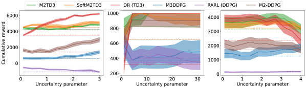
Figure 1: Cumulative rewards under trained policies for each uncertainty parameter $\omega\in\Omega$. The average (solid line) and standard error (band) for each $\omega\in\Omega$, as well as the worst average value (dashed line) are shown. Left: Ant 1, Middle: InvertedPendulum 1, Right: Walker 1.

Table 1 summarizes the worst-case performances of the policies trained by M2TD3, SoftM2TD3, M2-DDPG, M3DDPG, RARL, and DR. See also Table 7 in Appendix E for the results of TD3 trained on the reference uncertainty parameters as baselines and Figure 2 in Appendix G for the learning curves. In most cases, M2TD3 and SoftM2TD3 outperformed DR, and RARL, and M3DDPG. Figure 1 shows the cumulative rewards of the policies trained by the six approaches for each of the $\omega$ values on the Ant 1, InvertedPendulum 1, and Walker 1 senarios. See also Figure 4 in Appendix H for other senarios.

Comparison with DR: DR does not attempt to optimize the worst-case performance. In fact, it showed lower worst-case performance than M2TD3 and SoftM2TD3 in many scenarios because the obtained policy performs poorly on some uncertainty parameters while it performs well on average. In the results of InvertedPendulum 1 shown in Figure 1, for example, the policy obtained by DR exhibited a high performance for a wide range of $\omega\in\Omega$ but performed poorly for small $\omega$. M2TD3 outperformed DR and the other baselines on those senarios. However, in some scenarios, such as HumanoidStandup 1, Small HalfCheetah 1, and Small Hopper 1, DR achieved a better worst-case performance than M2TD3. This outcome may be because the optimization of worst-case function values is generally more unstable than that of the expected function values.

Comparison with RARL: M2-DDPG outperformed RARL in most senarios, with this performance difference originating from the different optimization strategies. As noted above, the optimization strategy employed in RARL often fails to converge. Specifically, as shown in Figure 1, RARL failed to optimize the policy not only in the worst-case but also on average in Ant 1 and Walker 1 senarios. In the InvertedPendulum 1 senario, RARL could train the policy for some uncertainty parameters, but not for the worst-case uncertainty parameter.

Comparison with M3DDPG: In many cases, M2-DDPG outperformed M3DDPG. Because M3DDPG considers a stronger adversary than necessary (the worst $\omega$ for each time step), it was too conservative for this experiment and exhibited lower performance.

Average Performance

Although our objective is maximizing the worst-case performance, the average performance is also important in practice. Table 2 compares the average performance of the six approaches. Generally, DR achieved the highest average performance as expected. However, interestingly, M2TD3 and SoftM2TD3 achieved competitive average performances to DR on several senarios such as Hopper 1, 2, and Walker 1, 2. Moreover, Table 1 compared with Table 2 shows that a few times higher average performance than worst-case performance on several senarios such as Ant 3 and Hopper 1–3.

Table 2: Avg. $\pm$ std. error of average performance $R_{\text{average}}(\mu)$ over 10 trials for each approach

Environment	M2TD3	SoftM2TD3	M2-DDPG	M3DDPG	RARL (DDPG)	DR (TD3)
Ant 1 $(\times 10^{3})$	$4.51\pm 0.08$	$4.78\pm 0.16$	$2.05\pm 0.21$	$0.84\pm 0.14$	$-0.82\pm 0.06$	$\bm{5.25\pm 0.10}$
Ant 2 $(\times 10^{3})$	$5.44\pm 0.05$	$5.56\pm 0.01$	$3.03\pm 0.19$	$1.86\pm 0.38$	$-1.00\pm 0.06$	$\bm{6.32\pm 0.09}$
Ant 3 $(\times 10^{3})$	$2.66\pm 0.22$	$2.98\pm 0.23$	$0.30\pm 0.46$	$-0.33\pm 0.22$	$-1.31\pm 0.09$	$\bm{3.62\pm 0.11}$
HalfCheetah 1 $(\times 10^{3})$	$3.89\pm 0.06$	$4.00\pm 0.05$	$3.50\pm 0.12$	$1.01\pm 0.26$	$-0.46\pm 0.02$	$\bm{5.93\pm 0.18}$
HalfCheetah 2 $(\times 10^{3})$	$4.35\pm 0.05$	$4.52\pm 0.07$	$3.91\pm 0.08$	$0.77\pm 0.12$	$-0.08\pm 0.05$	$\bm{5.79\pm 0.15}$
HalfCheetah 3 $(\times 10^{3})$	$3.79\pm 0.09$	$4.02\pm 0.04$	$3.39\pm 0.21$	$0.58\pm 0.18$	$-0.21\pm 0.10$	$\bm{5.54\pm 0.16}$
Hopper 1 $(\times 10^{3})$	$\bm{2.68\pm 0.11}$	$2.67\pm 0.18$	$1.79\pm 0.22$	$1.12\pm 0.21$	$0.38\pm 0.08$	$2.57\pm 0.15$
Hopper 2 $(\times 10^{3})$	$\bm{2.51\pm 0.07}$	$2.26\pm 0.12$	$1.49\pm 0.15$	$1.15\pm 0.11$	$0.66\pm 0.13$	$1.89\pm 0.08$
Hopper 3 $(\times 10^{3})$	$0.85\pm 0.07$	$0.79\pm 0.04$	$0.87\pm 0.08$	$0.49\pm 0.11$	$0.47\pm 0.08$	$\bm{1.50\pm 0.07}$
HumanoidStandup 1 $(\times 10^{5})$	$1.08\pm 0.04$	$1.03\pm 0.07$	$1.05\pm 0.06$	$0.99\pm 0.06$	$0.77\pm 0.06$	$\bm{1.12\pm 0.05}$
HumanoidStandup 2 $(\times 10^{5})$	$0.97\pm 0.04$	$\bm{1.07\pm 0.05}$	$0.93\pm 0.04$	$0.92\pm 0.04$	$0.85\pm 0.08$	$1.06\pm 0.04$
HumanoidStandup 3 $(\times 10^{5})$	$\bm{1.09\pm 0.06}$	$1.04\pm 0.03$	$0.98\pm 0.06$	$1.01\pm 0.04$	$0.87\pm 0.07$	$1.04\pm 0.07$
InvertedPendulum 1 $(\times 10^{2})$	$\bm{9.66\pm 0.25}$	$9.17\pm 0.54$	$8.79\pm 0.87$	$4.51\pm 0.12$	$4.21\pm 0.81$	$9.32\pm 0.11$
InvertedPendulum 2 $(\times 10^{2})$	$6.13\pm 1.42$	$6.26\pm 0.95$	$8.27\pm 0.70$	$1.76\pm 0.51$	$3.07\pm 0.66$	$\bm{9.18\pm 0.07}$
Walker 1 $(\times 10^{3})$	$\bm{3.70\pm 0.31}$	$3.51\pm 0.16$	$2.03\pm 0.26$	$1.55\pm 0.25$	$0.15\pm 0.03$	$3.59\pm 0.26$
Walker 2 $(\times 10^{3})$	$\bm{4.72\pm 0.12}$	$4.37\pm 0.32$	$2.39\pm 0.20$	$1.63\pm 0.22$	$0.26\pm 0.05$	$4.54\pm 0.31$
Walker 3 $(\times 10^{3})$	$4.27\pm 0.21$	$4.21\pm 0.30$	$2.48\pm 0.24$	$1.65\pm 0.15$	$0.21\pm 0.07$	$\bm{4.48\pm 0.16}$
Small HalfCheetah 1 $(\times 10^{3})$	$6.00\pm 0.15$	$6.04\pm 0.13$	$5.71\pm 0.07$	$3.38\pm 0.34$	$-0.42\pm 0.01$	$\bm{8.11\pm 0.17}$
Small Hopper 1 $(\times 10^{3})$	$2.96\pm 0.31$	$2.44\pm 0.31$	$1.57\pm 0.21$	$1.53\pm 0.21$	$0.56\pm 0.13$	$\bm{3.44\pm 0.10}$

Table 3: Avg. $\pm$ std. error of worst-case performance $R_{\text{worst}}(\mu)$ and average performance $R_{\text{average}}(\mu)$ on InvertedPendulum 1 obtained by M2TD3 variants over 10 trials

Environment	N=5	N=1	N=10	w/o DRS	w/o PRS
worst-case $(\times 10^{2})$	$8.22\pm 1.13$	$5.77\pm 1.29$	$9.07\pm 0.89$	$9.07\pm 0.88$	$5.41\pm 1.45$
average $(\times 10^{2})$	$9.66\pm 0.25$	$8.10\pm 0.90$	$9.89\pm 0.11$	$9.08\pm 0.88$	$6.90\pm 1.25$

Ablation Study

Ablation studies were conducted on InvertedPendulum 1 with the pole mass as the uncertainty parameters. M2TD3 with $N=5$ was taken as the baseline. We tested several variants as follows: with different multiple uncertainty parameters ($N=1$ and $10$), without a distance-based refreshing strategy (w/o DRS), and without a probability-based refreshing strategy (w/o PRS). Table 3 shows the results. The inclusion of multiple uncertainty parameters and the probability-based refresh strategy contributed significantly to the worst-case performance and average performance, implying that both techniques contribute to better estimating the worst uncertainty parameter. Although DRS had little impact on the performance, prior knowledge in DRS can be implemented by defining the distance and the threshold in the uncertainty parameter task-dependently, which we did not implement here.

Small Uncertainty Set (Limitation of M2TD3)

Small HalfCheetah 1 and Small Hopper 1 were designed to have a smaller uncertainty parameter set than HalfCheetah 1 and Hopper 1 and to reveal the effect of the size of the uncertainty parameter interval. As expected, a smaller uncertainty parameter set resulted in higher worst-case (Table 1) and average (Table 2) performances, for all approaches. Because M2TD3 performs the worst-case optimization, it is expected to show better worst-case performance than DR, independently of the size of the uncertainty parameter set. However, in these senarios, DR showed better worst-case performance than that of M2TD3, while M2TD3 achieved competitive or superior worst-case performance to those of DR on HalfCheetah 1 and Hopper 1. This may be because the max-min optimization performed by M2TD3 resulted in sub-optimal policies. When the uncertainty parameter set is small, and the performance does not change significantly over the uncertainty parameter set, maximizing the average performance is likely to lead to high worst-case performance. The sub-optimal results obtained by M2TD3 is then dominated by the results obtained by DR. Therefore, the maxmin optimization in M2TD3 can be improed.

Evaluation Under Adversarial External Force

Although we developed the proposed approach for the situation that the uncertainty parameter is directly encoded by $\omega$, we can extend it to the situation where the model misspecification is expressed by an external force produced by an adversarial agent as in [31]. The extended approach and its experimental result are given in Appendix J. Superior worst-case performances of M2TD3 over DR, RARL, and M3DDPG were observed for this setting as well.

6 Conclusion

In this study, we targeted the policy optimization aimed at maximizing the worst-case performance in a predefined uncertainty set. The list of the contributions are as follows. (i) We formulated the off-policy deterministic actor-critic approach to the worst-case performance maximization as a tri-level optimization problem (3). (ii) We developed the worst-case performance of M2TD3. The key concepts were the incorporation of the uncertainty parameter into the critic network and use of the simultaneous gradient ascent descent method. Different technical components were introduced to stabilize the training. (iii) We evaluated the worst-case performance of M2TD3 on 19 MuJoCo tasks through comparison with three baseline methods. Ablation studies revealed the usefulness of each component of M2TD3.

Checklist

1. For all authors…

   1. Do the main claims made in the abstract and introduction accurately reflect the paper’s contributions and scope? [Yes] Please see Section 3 and Section 5.

   2. Did you describe the limitations of your work? [Yes] Please see paragraph titled "Small Uncertainty Set" in Section 5 and Section 6.

   3. Did you discuss any potential negative societal impacts of your work? [N/A]

   4. Have you read the ethics review guidelines and ensured that your paper conforms to them? [Yes]

2. If you are including theoretical results…

   1. Did you state the full set of assumptions of all theoretical results? [N/A]

   2. Did you include complete proofs of all theoretical results? [N/A]

3. If you ran experiments…

   1. Did you include the code, data, and instructions needed to reproduce the main experimental results (either in the supplemental material or as a URL)? [Yes] Please see Appendix A.

   2. Did you specify all the training details (e.g., data splits, hyperparameters, how they were chosen)? [Yes] Please see Section 5 and Appendix C.

   3. Did you report error bars (e.g., w.r.t. the random seed after running experiments multiple times)? [Yes]

   4. Did you include the total amount of compute and the type of resources used (e.g., type of GPUs, internal cluster, or cloud provider)? [Yes] Please see Appendix C.

4. If you are using existing assets (e.g., code, data, models) or curating/releasing new assets…

   1. If your work uses existing assets, did you cite the creators? [Yes]

   2. Did you mention the license of the assets? [Yes] Code licence is part of the repository.

   3. Did you include any new assets either in the supplemental material or as a URL? [Yes] We include our code in the Appendix A.

   4. Did you discuss whether and how consent was obtained from people whose data you’re using/curating? [N/A]

   5. Did you discuss whether the data you are using/curating contains personally identifiable information or offensive content? [N/A]

5. If you used crowdsourcing or conducted research with human subjects…

   1. Did you include the full text of instructions given to participants and screenshots, if applicable? [N/A]

   2. Did you describe any potential participant risks, with links to Institutional Review Board (IRB) approvals, if applicable? [N/A]

   3. Did you include the estimated hourly wage paid to participants and the total amount spent on participant compensation? [N/A]

Appendix A Algorithm Details

Algorithm 2 summarizes the overall framework of M2TD3. The training is stalled if the size of the replay buffer is smaller than the minibatch size, i.e., if $\lvert B\rvert<M$. Algorithms 3 and 4 show the critic network update and the actor network and uncertainty parameter sampler update, respectively. Although we write the gradient-based update in the form of a mini-batch stochastic gradient update for simplicity, we employ an adaptive approach such as Adam [16].

Algorithm 2 M2TD3 (Framework)

1:  # initialization

2:  Initialize uncertainty parameters $\hat{\omega}_{i}\in\mathcal{U}(\Omega)$ for $i=1,\dots,N$

3:  Initialize policy parameter $\theta$ and critic parameters $\phi_{1}$, $\phi_{2}$ with random values

4:  Initialize target network parameters $\theta^{\prime}\leftarrow\theta$, $\phi_{1}^{\prime}\leftarrow\phi_{1}$, $\phi_{2}^{\prime}\leftarrow\phi_{2}$

5:  Initialize frequency parameter $p_{1},\dots,p_{N}=1/N$

6:  Initialize replay buffer $B=\emptyset$

7:  # training loop

8:  Draw uncertainty parameter $\omega\sim\alpha_{0}$

9:  Observe initial state $s\sim p_{\omega}^{0}$

10:  for $\mathrm{t}=1$ to $T_{\text{max}}$ do

11:     # interaction

12:     Select action $a\sim\beta_{t}(s)$

13:     Interact with $\mathcal{M}_{\omega}$ with $a$, observe next state $s^{\prime}$, immediate reward $r$ and termination flag $h$

14:     Store transition tuple $(s,a,r,s^{\prime},h,\omega)$ in $B$

15:     if $h=1$ then

16:        Reset uncertainty parameter $\omega\sim\alpha_{t}$

17:        Observe initial state $s\sim p_{\omega}^{0}$

18:     else

19:        Update current state $s\leftarrow s^{\prime}$

20:     end if

21:     # learning

22:     Sample mini-batch $\{(s_{i},a_{i},r_{i},s_{i}^{\prime},h_{i},\omega_{i})\}$ of $\mathrm{M}$ transitions uniform-randomly from $B$

23:     Perform Algorithm 3 for critic network update

24:     if $\mathrm{mod}(t,T_{\text{freq}})=0$ then

25:        Perform Algorithm 4 for actor network update and uncertainty parameter sampler update

26:        Update target networks analogously to TD3

27:     end if

28:  end for

Algorithm 3 Critic Update

1:  for $i=1,\dots,M$ do

2:     $\tilde{a}_{i}\leftarrow\mu_{\theta^{\prime}}(s_{i}^{\prime})+\epsilon_{a}$, $\epsilon_{a}\sim\Pi_{a}(\mathcal{N}(0,\tilde{\Sigma}_{a}))$

3:     $\tilde{\omega}_{i}^{\prime}\leftarrow\omega_{i}+\epsilon_{\omega}$, $\epsilon_{\omega}\sim\Pi_{\omega}(\mathcal{N}(0,\tilde{\Sigma}_{\omega}))$

4:     $y_{i}\leftarrow r_{i}+\min\{Q_{\phi^{\prime}_{1}}(s_{i}^{\prime},\tilde{a}_{i},\tilde{\omega}_{i}),Q_{\phi^{\prime}_{2}}(s_{i}^{\prime},\tilde{a}_{i},\tilde{\omega}_{i})\}$

5:  end for

6:  for $j=1,2$ do

7:     $\phi_{j}\leftarrow\phi_{j}-\lambda_{\phi}\nabla_{\phi_{j}}\frac{1}{M}\sum_{i=1}^{M}(y_{i}-Q_{\phi_{j}}(s_{i},a_{i},\omega_{i}))^{2}$

8:  end for

Algorithm 4 Actor Update and Uncertainty Parameter Sampler Update

1:  # maximin update

2:  $k^{\prime}=\operatornamewithlimits{argmin}_{k}\frac{1}{M}\sum_{i=1}^{M}Q_{\phi^{1}}(s_{i},\mu_{\theta}(s_{i}),\hat{\omega}_{k})$

3:  $\theta\leftarrow\theta+\lambda_{\theta}\nabla_{\theta}\frac{1}{M}\sum_{i=1}^{M}Q_{\phi^{1}}(s_{i},\mu_{\theta}(s_{i}),\hat{\omega}_{k^{\prime}})$

4:  $\hat{\omega}_{k^{\prime}}\leftarrow\hat{\omega}_{k^{\prime}}-\lambda_{\omega}\nabla_{\hat{\omega}_{k^{\prime}}}\frac{1}{M}\sum_{i=1}^{M}Q_{\phi^{1}}(s_{i},\mu_{\theta}(s_{i}),\hat{\omega}_{k^{\prime}})$

5:  # uncertainty parameter sampler update with refreshing strategy

6:  for $k=1,\dots,N$ do

7:     $\hat{\omega}_{k}\sim\mathcal{U}(\Omega)$ if $d_{\omega}(\hat{\omega}_{k},\hat{\omega}_{\ell})\leqslant d_{\mathrm{thre}}$ for some $\ell\neq k$

8:     $\hat{\omega}_{k}\sim\mathcal{U}(\Omega)$ if $p_{k}\leqslant p_{\mathrm{thre}}$

9:     if $\hat{\omega}_{k}$ is refreshed then

10:        $p_{k}\leftarrow 1/N$

11:     else

12:        $p_{k}\leftarrow(1-1/T_{\mathrm{last}})p_{k}+(1/T_{\mathrm{last}})\mathbb{I}\{k=k^{\prime}\}$

13:     end if

14:  end for

15:  $p_{k}\leftarrow p_{k}/\sum_{\ell=1}^{n}p_{\ell}$ for all $k=1,\dots,N$

We maintain the frequency $p_{k}$ of each uncertainty parameter $\hat{\omega}_{k}$ being the worst one among $\hat{\omega}_{1},\dots,\hat{\omega}_{N}$ in Algorithm 4. This is used in two ways: criteria for the refreshing strategy of $\hat{\omega}_{k}$ in Algorithm 4; and mixture weights for the uncertainty parameter sampler $\alpha$. The update of $p_{k}$ follows the exponential moving average with the momentum $(1/T_{\text{last}})$, where $T_{\text{last}}$ is the number of steps spent in the last episode ($T_{\text{last}}$ is set to $1000$ for the first episode). The reason behind this design choice is as follows. The short episode is a meaning that a bad uncertainty parameter $\omega$ is used in the last episode. Because the uncertainty parameter $\omega$ used in the interaction is sampled from $\alpha$, which is a gaussian mixture with components centered at $\hat{\omega}_{1},\dots,\hat{\omega}_{k}$, it implies that they include a bad uncertainty parameter as well. Then, there is a high chance that this uncertainty parameter is selected as the worst uncertainty parameter $\hat{\omega}_{k^{\prime}}$ in Algorithm 4. By setting a greater momentum $(1/T_{\text{last}})$, we can accelerate the approach of $p_{k}$ to $\mathbb{I}\{k=k^{\prime}\}$, which is $1$ if $k=k^{\prime}$ and $0$ otherwise. With this fast update of $p_{k}$, we expect two consequences. First, there are increased chances to sample $\omega$ around the worst $\hat{\omega}_{k^{\prime}}$. Second, there are increased chances to refresh the non-worst uncertainty parameters, which leads to more exploration of the worst uncertainty parameter search. Preliminary experiments have confirmed that this momentum setting leads to a better worst-case performance than a constant momentum.

Our implementation is publicly available (https://github.com/akimotolab/M2TD3).

Appendix B Soft-Min Variant: SoftM2TD3

In theory, M2TD3 can obtain a policy that exhibits a better worst-case performance than a policy obtained by DR as DR does not explicitly maximize the worst-case performance. However, we empirically observe that DR sometimes achieves a better worst-case performance than M2TD3 on senarios where the performance does not change significantly over the uncertainty set $\Omega$ (Table 1). We conjecture that this is because the difficulty in the max-min optimization of M2TD3 compared to the optimization of the expectation in DR.

To mitigate this issue, we propose a variant of M2TD3, called SoftM2TD3. The objective of the update of the policy parameter $\theta$ is replaced with the following soft-min version:

$$\tilde{J}_{t}(\theta) =\sum_{k=1}^{N}w_{k}\left[\frac{1}{M}\sum_{i=1}^{M}Q_{\phi_{t}}(s_{i},\mu_{\theta}(s),\hat{\omega}_{k})\right]\enspace,$$ (8)

where $w_{k}$ is the weight for uncertainty parameter $\hat{\omega}_{k}$. A greater weight value should be assigned to $\hat{\omega}_{k}$ with smaller Q-values. We used the frequency $p_{k}$ of $\hat{\omega}_{k}$ as the worst-case during the actor update, i.e., $w_{k}=p_{k}$. This update is close to M2TD3 if $p=(p_{1},\dots,p_{N})$ is close to a one-hot vector and is close to DR if $p_{1}\approx\cdots\approx p_{N}$, which is the case at the beginning of the training.

The objective function of SoftM2TD3 is considered an approximation of the objective function of M2TD3. The difference between M2TD3 and SoftM2TD3 is in the optimization process. Because the objective function of SoftM2TD3 is closer to that of DR, we expect that the optimization in SoftM2TD3 is more efficient than M2TD3, where the effect of the accuracy of the estimation of the worst-case uncertainty parameters is greater than SoftM2TD3.

Appendix C Experiment Details

Table 4: List of senarios used in the experiments

Environment	Uncertainty Set $\Omega$	Reference Parameter	Uncertainty Parameter Name
Baseline MuJoCo Environment: Ant
Ant 1	[0.1, 3.0]	0.33	torso mass
Ant 2	[0.1, 3.0] $\times$ [0.01, 3.0]	(0.33, 0.04)	torso mass $\times$ front left leg mass
Ant 3	[0.1, 3.0] $\times$ [0.01, 3.0] $\times$ [0.01, 3.0]	(0.33, 0.04, 0.06)	torso mass $\times$ front left leg mass $\times$ front right leg mass
Baseline MuJoCo Environment: HalfCheetah
HalfCheetah 1	[0.1, 4.0]	0.4	world friction
HalfCheetah 2	[0.1, 4.0] $\times$ [0.1, 7.0]	(0.4, 6.36)	world friction $\times$ torso mass
HalfCheetah 3	[0.1, 4.0] $\times$ [0.1, 7.0] $\times$ [0.1, 3.0]	(0.4, 6.36, 1.53)	world friction $\times$ torso mass $\times$ back thigh mass
Baseline MuJoCo Environment: Hopper
Hopper 1	[0.1, 3.0]	1.00	world friction
Hopper 2	[0.1, 3.0] $\times$ [0.1, 3.0]	(1.00, 3.53)	world friction $\times$ torso mass
Hopper 3	[0.1, 3.0] $\times$ [0.1, 3.0] $\times$ [0.1, 4.0]	(1.00, 3.53, 3.93)	world friction $\times$ torso mass $\times$ thigh mass
Baseline MuJoCo Environment: HumanoidStandup
HumanoidStandup 1	[0.1, 16.0]	8.32	torso mass
HumanoidStandup 2	[0.1, 16.0] $\times$ [0.1, 8.0]	(8.32, 1.77)	torso mass $\times$ right foot mass
HumanoidStandup 3	[0.1, 16.0] $\times$ [0.1, 5.0] $\times$ [0.1, 8.0]	(8.32, 1.77, 4.53)	torso mass $\times$ right foot mass $\times$ left thigh mass
Baseline MuJoCo Environment: Inveted Pendulum
InvertedPendulum 1	[1.0, 31.0]	4.90	pole mass
InvertedPendulum 2	[1.0, 31.0] $\times$ [1.0, 11.0]	(4.90, 9.42)	pole mass $\times$ cart mass
Baseline MuJoCo Environment: Walker
Walker 1	[0.1, 4.0]	0.7	world friction
Walker 2	[0.1, 4.0] $\times$ [0.1, 5.0]	(0.7, 3.53)	world friction $\times$ torso mass
Walker 3	[0.1, 4.0] $\times$ [0.1, 5.0] $\times$ [0.1, 6.0]	(0.7, 3.53, 3.93)	world friction $\times$ torso mass $\times$ thigh mass
Small MuJoCo Environments
Small HalfCheetah 1	[0.1, 3.0]	0.4	world friction
Small Hopper 1	[0.1, 2.0]	1.00	world friction

Table 4 lists the senario we used in our experiments. These senarios are created by setting 1 to 3 constants in the original MuJoCo environment to the uncertainty parameters. The uncertainty set is designed as an interval. Except for Hopper 2 and Hopper 3, the original value is included in the uncertainty set; hence, the trivial upper bound of the worst-case performance is the best performance of the corresponding MuJoCo environment.

In all approaches in all senarios, the same configurations are used for fair comparison as follows.

For DR and RARL, the input to the critic is a $(s,a)$ pair, whereas it is a tuple of $(s,a,\omega)$ for M2TD3, SoftM2TD3, and M3DDPG. Except for this point, we used the same network architecture. The policy and the critic networks are defined as fully connected layers with two hidden layers of size 256.

The uncertainty parameter sampler $\alpha_{t}$ is

$$\alpha_{t}=\begin{cases}\mathcal{U}(\Omega)&t\leqslant T_{\text{rand}}\\ \Pi_{\Omega}(\sum_{k=1}^{N}p_{k}\cdot\mathcal{N}(\hat{\omega}_{k},\Sigma_{\omega}))&t>T_{\text{rand}}\enspace,\end{cases}$$ (9)

where $\Sigma_{\omega}$ is a diagonal matrix, with diagonal elements 0.5 times the lengths of the intervals of the corresponding dimension of $\Omega$, and $\Pi_{\Omega}$ is the projection onto $\Omega$ and $T_{\text{rand}}=10^{5}$. The behavior policy $\beta_{t}$ is

$$\beta_{t}=\begin{cases}\mathcal{U}(A)&t\leqslant T_{\text{rand}}\\ \Pi_{A}(\mathcal{N}(\mu_{\theta}(s),\Sigma_{a}))&t>T_{\text{rand}}\enspace,\end{cases}$$ (10)

where $\Sigma_{a}$ is a diagonal matrix, with diagonal elements are the 0.5 times the length of the intervals of the corresponding dimension of $A$, and $\Pi_{A}$ is the projection onto $A$. The $\Sigma_{\omega}$ element is designed to decay at each time step to 0.05 times the length of the intervals of it when the learning progresses to half of the total.

The minibatch size is $M=100$. The learning rates for the actor update, the uncertainty parameter update and the critic update are $\lambda_{\theta}=\lambda_{\omega}=\lambda_{\phi}=3\times 10^{-4}$. The noise covariance matrices for the target policy smoothing are $\tilde{\Sigma}_{a}=2\Sigma_{a}$ and $\tilde{\Sigma}_{\omega}=2\Sigma_{\omega}$. The noise for the target policy smoothing is clipped by $\Pi_{a}$ and $\Pi_{\omega}$ into the ranges of $\pm 0.25$ times the interval lengths of the corresponding dimensions of $A$ and $\Omega$, respectively. The actor and target network update frequency is $T_{\text{freq}}=2$. The above parameter settings follow TD3 [7].

We used $N=5$ uncertainty parameters. For the refreshing strategy of the uncertainty parameters, we used $\ell_{1}$-distance as $d_{\omega}$. The distance threshold is $d_{\mathrm{thre}}=0.1$. The frequency threshold is $0.05$.

Experiments were performed on a machine with two NVIDIA RTX A5000 GPUs, two Intel(R) Xeon(R) Gold 6230 CPUs, and 192GB memory.

Appendix D Related Work

Table 5 summarizes the robust policy search method taxonomy. Table 6 compares the related methods considering their action value function definitions.

Table 5: Taxonomy of robust policy search. Cont.: Continuous space. Disc.: Discrete space.

Method	Uncertainty	$S$ & $A$	$\Omega$
R-MPO	Transition	Cont.	Disc.
ROPI	Transition	Disc.	Cont.
ATLA, SA-DRL	Observation	Cont.	Cont.
PAIRED, RARL, M3DDPG RRL, Adv-SAC, RSAC, M2TD3	Reward & Transition	Cont.	Cont.

Table 6: Comparison of action value functions in related methods

Method	Action Value Function
R-MPO, ROPI, Robust DP	$Q(s,a)=r(s,a)+\gamma\min_{\omega\in\Omega}\mathbb{E}[Q(s^{\prime},\mu_{\theta}(s^{\prime}))\mid s^{\prime}\sim p_{\omega}(\cdot\mid s,a)]$
DR	$Q(s,a)=\mathbb{E}_{\omega\in\Omega}[r_{\omega}(s,a)+\gamma\mathbb{E}[Q(s^{\prime},\mu_{\theta}(s^{\prime}))\mid s^{\prime}\sim p_{\omega}(\cdot\mid s,a)]]$
RRL, RARL, Adv-SAC	$Q_{\omega}(s,a)=r_{\omega}(s,a)+\gamma\mathbb{E}[Q_{\omega}(s^{\prime},\mu_{\theta}(s^{\prime}))\mid s^{\prime}\sim p_{\omega}(\cdot\mid s,a)]$
M3DDPG	$Q(s,a,\omega)=r_{\omega}(s,a)+\gamma\mathbb{E}[\min_{\omega^{\prime}\in\Omega}Q(s^{\prime},\mu_{\theta}(s^{\prime}),\omega^{\prime})\mid s^{\prime}\sim p_{\omega}(\cdot\mid s,a)]$
M2TD3	$Q(s,a,\omega)=r_{\omega}(s,a)+\gamma\mathbb{E}[Q(s^{\prime},\mu_{\theta}(s^{\prime}),\omega)\mid s^{\prime}\sim p_{\omega}(\cdot\mid s,a)]$

Appendix E Performance of TD3

Table 7: Avg. $\pm$ std. error of worst-case performance $R_{\text{worst}}(\mu)$ and average performance $R_{\text{average}}(\mu)$ and reference performance $R_{\text{ref}}(\mu)$ over 10 trials for TD3 (reference parameter)

Environment	worst	average
Ant (reference parameters): $3.02\pm 0.15(\times 10^{3})$
Ant 1 $(\times 10^{3})$	$2.22\pm 0.50$	$2.76\pm 0.50$
Ant 2 $(\times 10^{3})$	$1.59\pm 0.08$	$2.28\pm 0.09$
Ant 3 $(\times 10^{2})$	$-0.99\pm 1.13$	$3.16\pm 1.00$
HalfCheetah (reference parameters): $10.2\pm 0.2(\times 10^{3})$
Small HalfCheetah 1 $(\times 10^{3})$	$0.03\pm 0.11$	$3.73\pm 0.29$
HalfCheetah 1 $(\times 10^{3})$	$-0.34\pm 0.04$	$2.79\pm 0.22$
HalfCheetah 2 $(\times 10^{3})$	$-0.53\pm 0.06$	$2.63\pm 0.20$
HalfCheetah 3 $(\times 10^{3})$	$-0.61\pm 0.08$	$2.47\pm 0.18$
Hopper (reference parameters): $3.01\pm 0.19(\times 10^{3})$
Small Hopper 1 $(\times 10^{3})$	$2.84\pm 0.22$	$2.97\pm 0.21$
Hopper 1 $(\times 10^{3})$	$0.40\pm 0.02$	$2.39\pm 0.14$
Hopper 2 $(\times 10^{3})$	$0.21\pm 0.04$	$1.54\pm 0.17$
Hopper 3 $(\times 10^{3})$	$0.14\pm 0.03$	$1.15\pm 0.14$
HumanoidStandup (reference parameters): $1.08\pm 0.03(\times 10^{5})$
HumanoidStandup 1 $(\times 10^{5})$	$0.85\pm 0.07$	$1.03\pm 0.04$
HumanoidStandup 2 $(\times 10^{5})$	$0.73\pm 0.07$	$1.03\pm 0.03$
HumanoidStandup 3 $(\times 10^{5})$	$0.57\pm 0.04$	$1.01\pm 0.03$
InvertedPendulum (reference parameters): $10.0\pm 0.0(\times 10^{2})$
InvertedPendulum 1 $(\times 10^{2})$	$0.24\pm 0.10$	$7.34\pm 0.76$
InvertedPendulum 2 $(\times 10^{2})$	$0.03\pm 0.00$	$4.05\pm 0.52$
Walker (reference parameters): $4.08\pm 0.16(\times 10^{3})$
Walker 1 $(\times 10^{3})$	$0.68\pm 0.12$	$3.12\pm 0.20$
Walker 2 $(\times 10^{3})$	$0.28\pm 0.07$	$2.70\pm 0.20$
Walker 3 $(\times 10^{3})$	$0.17\pm 0.06$	$2.60\pm 0.18$

Table 7 summarizes the worst-case performance and the average performance of the policies obtained by TD3 on the Ant, HalfCheetah, Hopper, HumanoidStandup, InvertedPendulum, and Walker environments with their reference parameters. The results show that the original TD3 policies learned under the reference parameter cannot be generalized to uncertain parameters set in most scenarios. These results provide the baseline performances on these environments and show that these environments are non-trivial for the worst-case and the average performance maximization.

Appendix F Original RARL

The performance of the original RARL, whose baseline RL approach is TRPO, is shown in Table 8. RARL (TRPO) exhibited low worst-case performances, similarly to those of RARL (DDPG). These low performances of RARL (TRPO) may be due to its defect of the optimization strategy and because TRPO is an on-policy method, which often requires a greater number of interactions than off-policy methods [10].

Table 8: Avg. $\pm$ std. error of worst-case performance $R_{\text{worst}}(\mu)$ and average performance $R_{\text{average}}(\mu)$ over 10 trials for RARL (TRPO)

Environment	worst	average
Ant 1 $(\times 10^{1})$	$-4.92\pm 0.48$	$-2.29\pm 0.22$
Ant 2 $(\times 10^{2})$	$-1.15\pm 0.19$	$-0.37\pm 0.04$
Ant 3 $(\times 10^{2})$	$-0.32\pm 0.41$	$1.28\pm 0.68$
HalfCheetah 1 $(\times 10^{2})$	$-3.06\pm 0.85$	$1.22\pm 0.63$
HalfCheetah 2 $(\times 10^{2})$	$-5.23\pm 0.89$	$-0.03\pm 0.73$
HalfCheetah 3 $(\times 10^{2})$	$-9.70\pm 1.89$	$-0.70\pm 0.65$
Hopper 1 $(\times 10^{2})$	$2.89\pm 0.25$	$3.49\pm 0.38$
Hopper 2 $(\times 10^{2})$	$2.67\pm 0.26$	$4.82\pm 0.64$
Hopper 3 $(\times 10^{2})$	$0.71\pm 0.13$	$2.24\pm 0.47$
HumanoidStandup 1 $(\times 10^{4})$	$5.30\pm 0.22$	$6.78\pm 0.21$
HumanoidStandup 2 $(\times 10^{4})$	$5.04\pm 0.09$	$6.99\pm 0.25$
HumanoidStandup 3 $(\times 10^{4})$	$4.99\pm 0.08$	$6.64\pm 0.17$
InvertedPendulum 1 $(\times 10^{2})$	$0.44\pm 0.10$	$3.03\pm 0.98$
InvertedPendulum 2 $(\times 10^{2})$	$0.16\pm 0.05$	$5.86\pm 0.87$
Walker 1 $(\times 10^{2})$	$2.96\pm 0.16$	$3.79\pm 0.34$
Walker 2 $(\times 10^{2})$	$2.53\pm 0.22$	$4.16\pm 0.34$
Walker 3 $(\times 10^{2})$	$2.82\pm 0.17$	$3.90\pm 0.14$
Small HalfCheetah 1 $(\times 10^{2})$	$-0.89\pm 0.80$	$3.44\pm 0.95$
Small Hopper 1 $(\times 10^{2})$	$4.37\pm 0.40$	$4.44\pm 0.42$

Appendix G Learning Curve

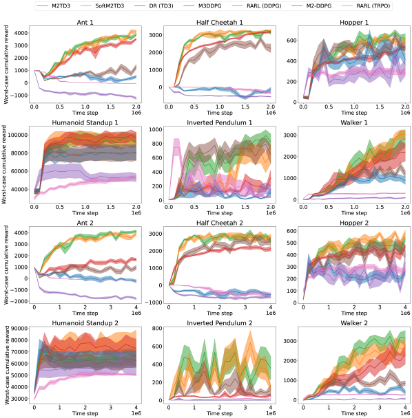
Figure 2: Learning curve for worst-case performance: the average (solid line) and standard error (band) of the worst-case cumulative rewards $R_{\text{worst}}(\mu)$

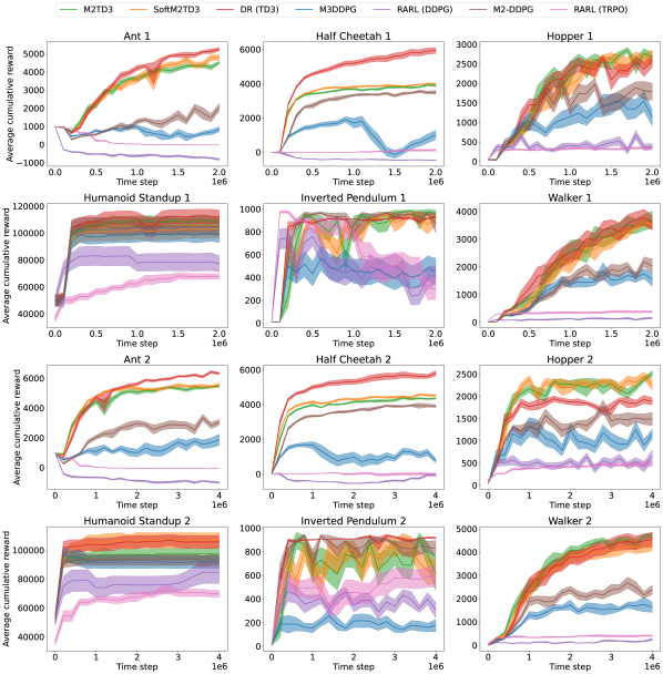
Figure 3: Learning curve for average performance: the average (solid line) and standard error (band) of the average cumulative rewards $R_{\text{average}}(\mu)$

The learning curves for each approach are shown in the Figure 2 and Figure 3. Figure 2 shows that M2TD3 and SoftM2TD3 tended to perform better in the early stages of learning than DR, even in scenarios where the final worst-case performances of DR, M2TD3, and SoftM2TD3 were competitive.

Appendix H Cumulative Rewards Under Different Uncertainty Parameters

Figures 4, 5 and 6 show the cumulative rewards of the policies trained by the seven approaches for each $\omega\in\Omega$. These results show that in many scenarios, DR achieved good performances in a wide range of uncertainty parameters. However, the differences between the worst-case and best-case performances were relatively large for DR, and the worst-case performances were relatively low. Unlike DR, M2TD3 exhibited smaller performance differences between the worst-case and the best-case, and its worst-case performances were relatively high.

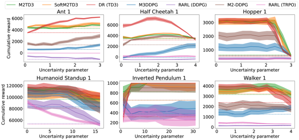
Figure 4: Cumulative rewards under trained policies for each uncertainty parameter $\omega\in\Omega$. The average (solid line) and standard error (band) for each $\omega\in\Omega$, as well as the worst average value (dashed line) are shown.

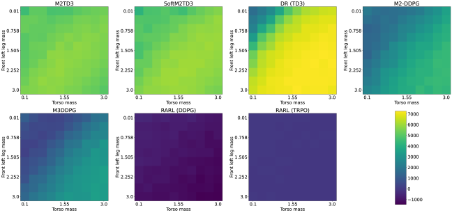
(a) Ant 2

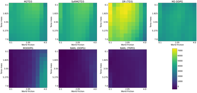
(b) HalfCheetah 2

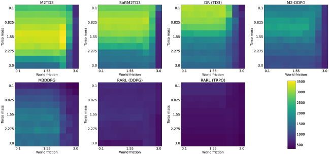
(c) Hopper 2

Figure 5: Cumulative rewards under trained policies for each uncertainty parameter $\omega\in\Omega$.

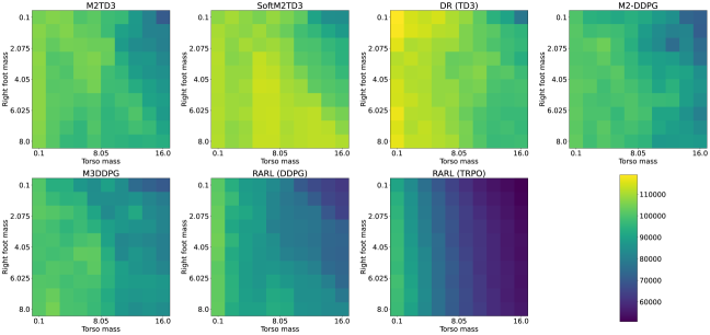
(a) HumanoidStandup 2

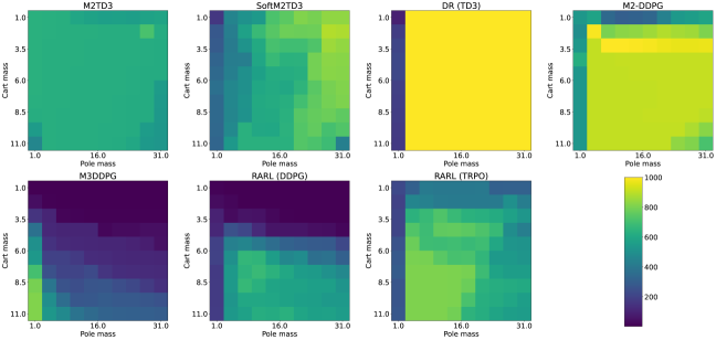
(b) InvertedPendulum 2

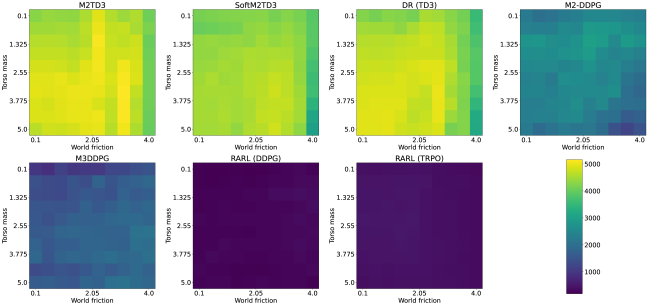
(c) Walker 2

Figure 6: Cumulative rewards under trained policies for each uncertainty parameter $\omega\in\Omega$.

Appendix I Multiple Uncertainty Parameter

Figure 7 shows the learning curves for each uncertainty parameter $\omega\in\Omega$ and the uncertainty parameter $\hat{\omega}$ used to update the actor ($\hat{\omega}_{k^{\prime}}$ in Algorithm 4) at each time step during the training. For each senario, the cumulative rewards under 10 equally spaced uncertainty parameters were evaluated every $1e5$ time steps. Hence, the lowest cumulative reward at each time step is a rough estimate of the worst-case performance. The uncertainty parameter with the lowest Q-value, $\operatornamewithlimits{argmin}_{\hat{\omega}_{1},\ldots,\hat{\omega}_{k},\ldots\hat{\omega}_{N}}J_{t}(\theta,\hat{\omega}_{k})$, is chosen for the update of the actor among $N$ worst uncertainty parameter candidates. This means that the selected worst-case uncertainty parameter can be different from the ground truth worst-case uncertainty parameter because of incomplete optimization for the worst uncertainty parameter, incomplete training of the critic network, and discrepancy between the cumulative reward and the Q-values.

Focusing on the behavior of M2TD3 on the HalfCheetah 1 senario (left-most side figures), the cumulative reward (top figure) shows that the uncertainty parameters $0.1$ (green line), $0.5$ (orange line), and $4.0$ (light blue line) alternately came to the bottom during learning, indicating that the worst uncertainty parameter continues to change between these values. The uncertainty parameter selected during the actor training (bottom figure) were the values around $0.1$ and $4.0$in the early stages of the training, and the values around $0.5$ were used in the middle of the training. This indicates that the algorithm was able to track the change of the worst-case uncertainty parameter during the training. This behavior of M2TD3 and SoftM2TD3 is shown on the other tasks.

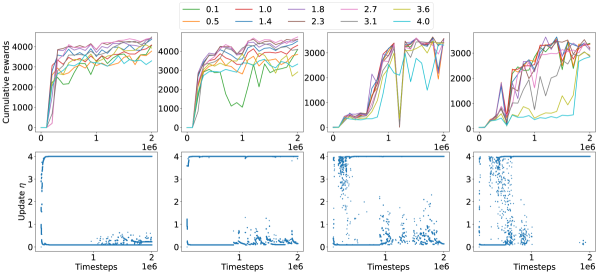
Figure 7: Cumulative reward under each uncertainty parameter (upper). Uncertainty parameter used to update at each time step (under). From left to right (scenario, algorithm): (HalfCheetah 1, M2TD3), (HalfCheetah 1, SoftM2TD3), (Walker 1, M2TD3), (Walker 1, SoftM2TD3).

Appendix J Evaluation Under Adversarial External Force

With a small modification of the proposed approaches, we can apply it to the situation conforming to [31], where the model misspecification is expressed by an external force given by an adversarial agent. In this section, we describe the necessary modification of the proposed approaches and compare the worst-case performance with baselines.

Extension of M2TD3

In this setting, we deal with an MDP $\mathcal{M}=\langle S,A_{p},A_{a},p,p_{0},r,\gamma\rangle$, where $A_{p}$ and $A_{a}$ are the action spaces of the protagonist agent and adversarial agent, respectively, and they are assumed to be continuous. The transition probability density $p:S\times A_{p}\times A_{a}\times S\rightarrow\mathbb{R}$ and immediate reward $r:S\times A_{p}\times A_{a}\rightarrow\mathbb{R}$ are not anymore parameterized by $\omega$ but take the action of the adversarial agent as input. Unless otherwise specified, the other notations are the same as the ones in Section 2. The protagonist and adversarial agents interact with the environment $\mathcal{M}$ using stochastic behavior policies $\beta$ and $\alpha$, respectively. Let $\rho^{\beta}_{\alpha}(s)=\lim_{T\rightarrow\infty}\frac{1}{T}\Sigma_{t=0}^{T-1}\int_{s_{0}}q^{t}_{\alpha,\beta}(s\mid s_{0})p_{0}(s_{0})\mathrm{d}s_{0}$ represent the stationary distribution of $s$ under $\beta$ and $\alpha$, where the step-$t$ transition probability density $q^{t}_{\alpha,\beta}$ is defined as $q^{1}_{\alpha,\beta}(s^{\prime}|s)=\int_{a^{p}\in A_{p}}\int_{a^{a}\in A_{a}}q(s^{\prime}|s,a^{p},a^{a})\beta(a^{p}|s)\alpha(a^{a}|s)\mathrm{d}a_{a}\mathrm{d}a_{p}$ and $q^{t}_{\alpha,\beta}(s^{\prime}|s)=\int_{\bar{s}\in S}q^{t-1}_{\alpha,\beta}(\bar{s}|s)q^{1}_{\alpha,\beta}(s^{\prime}|\bar{s})\mathrm{d}\bar{s}$. The joint stationary distribution of $(s,a^{p},a^{a})$ is defined as $\rho^{\beta}_{\alpha}(s,a^{p},a^{a})=\beta(a^{p}|s)\alpha(a^{a}|s)\rho^{\beta}_{\alpha}(s)$.

We extend the action value function as a function of state $s$, protagonist agent’s action $a^{p}$, and adversarial agent’s action $a^{a}$, namely,

$$Q^{\mu}_{\xi}(s,a^{p},a^{a})\\ =\mathbb{E}[R_{t}\mid s_{t}=s,a_{t}^{p}=a^{p},a_{t}^{a}=a^{a},s_{t+k+1}\sim q(\cdot\mid s_{t+k},\mu(s_{t+k}),\xi(s_{t+k}))\ \forall k\geqslant 0]\enspace,$$ (11)

where $\mu$ and $\xi$ represent the policies of the protagonist agent and the adversarial agent, respectively, to be trained. We suppose that they are parameterized by $\theta_{p}$ and $\theta_{a}$, respectively.

The objective of M2TD3 is extended as

$$\max_{\theta_{p}\in\Theta}\min_{\theta_{a}\in\Theta}J(\theta_{p},\theta_{a};\phi^{*})\quad\text{s.t.}\quad\phi^{*}\in\operatornamewithlimits{argmin}_{\phi\in\Phi}L(\phi;\theta_{p},\theta_{a})\enspace,$$ (12)

where the critic loss function $L$ is extended as

$$L(\phi,\theta_{p},\theta_{a}):=\int_{s\in S}\int_{a^{p}\in A_{p}}\int_{a^{a}\in A_{a}}(T^{\mu_{\theta_{p}}}_{\xi_{\theta_{a}}}[Q_{\phi}](s,a^{p},a^{a})-Q_{\phi}(s,a^{p},a^{a}))^{2}\\ \times\rho^{\beta}_{\alpha}(s,a^{p},a^{a})\mathrm{d}s\mathrm{d}a^{p}\mathrm{d}a^{a}\enspace,$$ (13)

where $T^{\mu_{\theta_{p}}}_{\xi_{\theta_{a}}}$ is a function satisfying

$$T^{\mu_{\theta_{p}}}_{\xi_{\theta_{a}}}[Q](s,a^{p},a^{a})=r_{\omega}(s,a^{p},a^{a})+\gamma\int_{s^{\prime}\in S}Q(s^{\prime},\mu_{\theta_{p}}(s^{\prime}),\xi_{\theta_{a}}(s^{\prime}))q(s^{\prime}|s,a^{p},a^{a})\mathrm{d}s^{\prime}\enspace.$$ (14)

The max-min objective function $J$ of the actor network is defined as

$$J(\theta_{p},\theta_{a};\phi):=\int_{s\in S}Q_{\phi}(s,\mu_{\theta_{p}}(s),\xi_{\theta_{a}}(s))\rho^{\beta}_{\alpha}(s)\mathrm{d}s\enspace,$$ (15)

and $\rho^{\beta}_{\alpha}(s,a^{p},a^{a})$ and $\rho^{\beta}_{\alpha}(s)$ are approximated by the replay buffer $B$ that stores the trajectories obtained by the interaction using $\beta$ and $\alpha$. Let $\{(s_{i},a^{p}_{i},a^{a}_{i},r_{i},s^{\prime}_{i})\}_{i=1}^{M}\subset B$ be mini-batch samples taken uniformly randomly from the replay buffer. The approximated objective function used for the critic update is

$$\tilde{L}(\phi) =\frac{1}{M}\sum_{i=1}^{M}(y_{i}-Q_{\phi}(s_{i},a^{p}_{i},a^{a}_{i}))^{2},$$ (16)

where $y_{i}=r_{i}+\gamma\cdot Q_{\phi}(s_{i}^{\prime},\mu_{\theta_{p}}(s_{i}^{\prime}),\xi_{\theta_{a}}(s_{i}^{\prime}))$. The approximated objective function used for the actor update is

$$\tilde{J}(\theta_{p},\theta_{a})=\frac{1}{M}\sum_{i=1}^{M}Q_{\phi}(s_{i},\mu_{\theta_{p}}(s_{i}),\xi_{\theta_{a}}(s_{i}))\enspace.$$ (17)

Replacing (6) and (7) with above defined functions, we obtain M2TD3 for this setting.

Experiment

We used the tasks provided in [31]. For each trained policy, the worst-case performance is estimated by fixing the trained policy of the protagonist agent and training the adversarial agent’s policy to minimize the protagonist agent’s performance. To evaluate the worst-case performance of each approach, we performed $5$ independent training for $2\times 10^{6}$ time steps for each approach. The trial is indexed as $n\in\{1,\dots,5\}$. Then, for each obtained protagonist policy, we trained the adversarial policy for $2\times 10^{6}$ time steps. We performed the adversarial policy training three times, and they are indexed as $m\in\{1,2,3\}$. During the training of the adversarial policy, we recorded the performance of the protagonist agent under the adversarial policy at time step $et\in\{10^{5},2\times 10^{5},\dots,2\times 10^{6}\}$ (every $10^{5}$ time steps), denoted as $R(\mu,\xi_{m,et})$. Then, the worst-case performance of a protagonist policy $\mu$ was estimated by $R_{\text{worst}}(\mu)=\min_{m=1,2,3}\min_{et\in\{10^{5},2\times 10^{5},\dots,2\times 10^{6}\}}R(\mu,\xi_{m,et})$. The average and standard error of $R_{\text{worst}}(\mu)$ over $5$ trials are reported for each approach. The parameters and network architecture of the protagonist agent used in all methods and the adversarial agents used in M2TD3, M2-DDPG, M3DDPG, RARL (TD3), and RARL (TRPO) are the same as in the situation that the uncertainty parameter is directly encoded by $\omega$. In the situation that the uncertainty parameter was directly encoded by $\omega$, multiple uncertainty parameters were trained, but in this setting, only one adversarial agent was trained. The adversarial TD3 agents used to estimate worst-case performance were similar to the parameters and network architecture used in [7].

The result is shown in Table 9.

M2TD3 showed better worst-case performance than DR in all but the HalfCheetahAdv-v1 senarios. The reference performances were comparable to those of DR. Compared to those of RARL, M2TD3 showed competitive or superior performances, both in the worst-case and reference-case. Comparing M2-DDPG (the proposed approach based on DDPG instead of TD3) and M3DDPG, we observed similar performances in many scenarios in both reference-case and worst-case, and M2-DDPG significantly outperformed M3DDPG on HopperAdv-v1.

Table 9: Avg. $\pm$ std. error of reference performance (performance under no disturbance) and worst-case performance over five trials for each approach

	TD3	DR	M2TD3	M2-DDPG	M3DDPG	RARL (TD3)	RARL (TRPO)
MuJoCo Environment: HalfCheetahAdv-v1 ($\times 10^{4}$)
reference	$1.13\pm 0.09$	$1.21\pm 0.03$	$1.15\pm 0.09$	$1.19\pm 0.04$	$1.21\pm 0.03$	$1.04\pm 0.09$	$0.68\pm 0.27$
worst-case	$1.02\pm 0.11$	$1.12\pm 0.05$	$1.07\pm 0.09$	$1.13\pm 0.06$	$1.13\pm 0.02$	$1.00\pm 0.10$	$0.33\pm 0.32$
MuJoCo Environment: HopperAdv-v1 ($\times 10^{3}$)
reference	$3.48\pm 0.16$	$3.55\pm 0.14$	$3.25\pm 0.56$	$2.63\pm 0.52$	$1.66\pm 0.33$	$2.42\pm 0.94$	$0.29\pm 0.07$
worst-case	$0.50\pm 0.13$	$1.79\pm 1.25$	$2.64\pm 0.84$	$2.16\pm 0.53$	$0.69\pm 0.23$	$0.82\pm 0.45$	$0.26\pm 0.08$
MuJoCo Environment: InvertedPendulumAdv-v1 ($\times 10^{3}$)
reference	$1.00\pm 0.00$	$1.00\pm 0.00$	$1.00\pm 0.00$	$1.00\pm 0.00$	$1.00\pm 0.00$	$0.63\pm 0.46$	$0.10\pm 0.07$
worst-case	$0.03\pm 0.01$	$0.23\pm 0.39$	$0.83\pm 0.35$	$0.70\pm 0.31$	$0.80\pm 0.38$	$0.04\pm 0.01$	$0.03\pm 0.01$
MuJoCo Environment: SwimmerAdv-v1 ($\times 10^{2}$)
reference	$1.42\pm 0.09$	$1.22\pm 0.25$	$1.38\pm 0.09$	$1.51\pm 0.10$	$1.51\pm 0.06$	$1.21\pm 0.05$	$0.21\pm 0.10$
worst-case	$0.96\pm 0.15$	$0.60\pm 0.48$	$1.14\pm 0.08$	$1.19\pm 0.04$	$1.21\pm 0.04$	$0.80\pm 0.05$	$-0.71\pm 0.37$
MuJoCo Environment: Walker2dAdv-v1 ($\times 10^{3}$)
reference	$4.18\pm 0.44$	$4.27\pm 0.61$	$4.59\pm 1.05$	$2.81\pm 0.81$	$2.26\pm 0.50$	$3.95\pm 0.27$	$0.32\pm 0.08$
worst-case	$3.74\pm 0.59$	$3.61\pm 0.93$	$4.26\pm 1.04$	$1.75\pm 0.62$	$1.63\pm 0.32$	$3.11\pm 0.13$	$0.14\pm 0.08$

References

- [1] Abbas Abdolmaleki, Jost Tobias Springenberg, Yuval Tassa, Rémi Munos, Nicolas Heess, and Martin A. Riedmiller. Maximum a posteriori policy optimisation. In 6th International Conference on Learning Representations, ICLR 2018, Vancouver, BC, Canada, April 30 - May 3, 2018, Conference Track Proceedings. OpenReview.net, 2018.
- [2] Anurag Ajay, Jiajun Wu, Nima Fazeli, Maria Bauzá, Leslie Pack Kaelbling, Joshua B. Tenenbaum, and Alberto Rodriguez. Augmenting physical simulators with stochastic neural networks: Case study of planar pushing and bouncing. In 2018 IEEE/RSJ International Conference on Intelligent Robots and Systems, IROS 2018, Madrid, Spain, October 1-5, 2018, pages 3066–3073. IEEE, 2018.
- [3] Erwin Coumans et al. Bullet physics library. Open source: bulletphysics. org, 15(49):5, 2013.
- [4] Constantinos Daskalakis, Stratis Skoulakis, and Manolis Zampetakis. The complexity of constrained min-max optimization. In Samir Khuller and Virginia Vassilevska Williams, editors, STOC ’21: 53rd Annual ACM SIGACT Symposium on Theory of Computing, Virtual Event, Italy, June 21-25, 2021, pages 1466–1478. ACM, 2021.
- [5] Michael Dennis, Natasha Jaques, Eugene Vinitsky, Alexandre M. Bayen, Stuart Russell, Andrew Critch, and Sergey Levine. Emergent complexity and zero-shot transfer via unsupervised environment design. In Hugo Larochelle, Marc’Aurelio Ranzato, Raia Hadsell, Maria-Florina Balcan, and Hsuan-Tien Lin, editors, Advances in Neural Information Processing Systems 33: Annual Conference on Neural Information Processing Systems 2020, NeurIPS 2020, December 6-12, 2020, virtual, 2020.
- [6] Omar Darwiche Domingues, Pierre Ménard, Emilie Kaufmann, and Michal Valko. Episodic reinforcement learning in finite mdps: Minimax lower bounds revisited. In Vitaly Feldman, Katrina Ligett, and Sivan Sabato, editors, Algorithmic Learning Theory, 16-19 March 2021, Virtual Conference, Worldwide, volume 132 of Proceedings of Machine Learning Research, pages 578–598. PMLR, 2021.
- [7] Scott Fujimoto, Herke van Hoof, and David Meger. Addressing function approximation error in actor-critic methods. In Jennifer G. Dy and Andreas Krause, editors, Proceedings of the 35th International Conference on Machine Learning, ICML 2018, Stockholmsmässan, Stockholm, Sweden, July 10-15, 2018, volume 80 of Proceedings of Machine Learning Research, pages 1582–1591. PMLR, 2018.
- [8] Florian Golemo, Adrien Ali Taïga, Aaron C. Courville, and Pierre-Yves Oudeyer. Sim-to-real transfer with neural-augmented robot simulation. In 2nd Annual Conference on Robot Learning, CoRL 2018, Zürich, Switzerland, 29-31 October 2018, Proceedings, volume 87 of Proceedings of Machine Learning Research, pages 817–828. PMLR, 2018.
- [9] Ian J. Goodfellow, Jean Pouget-Abadie, Mehdi Mirza, Bing Xu, David Warde-Farley, Sherjil Ozair, Aaron C. Courville, and Yoshua Bengio. Generative adversarial nets. In Zoubin Ghahramani, Max Welling, Corinna Cortes, Neil D. Lawrence, and Kilian Q. Weinberger, editors, Advances in Neural Information Processing Systems 27: Annual Conference on Neural Information Processing Systems 2014, December 8-13 2014, Montreal, Quebec, Canada, pages 2672–2680, 2014.
- [10] Tuomas Haarnoja, Aurick Zhou, Pieter Abbeel, and Sergey Levine. Soft actor-critic: Off-policy maximum entropy deep reinforcement learning with a stochastic actor. In Jennifer G. Dy and Andreas Krause, editors, Proceedings of the 35th International Conference on Machine Learning, ICML 2018, Stockholmsmässan, Stockholm, Sweden, July 10-15, 2018, volume 80 of Proceedings of Machine Learning Research, pages 1856–1865. PMLR, 2018.
- [11] Shariq Iqbal and Fei Sha. Actor-attention-critic for multi-agent reinforcement learning. In Kamalika Chaudhuri and Ruslan Salakhutdinov, editors, Proceedings of the 36th International Conference on Machine Learning, ICML 2019, 9-15 June 2019, Long Beach, California, USA, volume 97 of Proceedings of Machine Learning Research, pages 2961–2970. PMLR, 2019.
- [12] Garud N. Iyengar. Robust dynamic programming. Math. Oper. Res., 30(2):257–280, 2005.
- [13] Pingcheng Jian, Chao Yang, Di Guo, Huaping Liu, and Fuchun Sun. Adversarial skill learning for robust manipulation. In IEEE International Conference on Robotics and Automation, ICRA 2021, Xi’an, China, May 30 - June 5, 2021, pages 2555–2561. IEEE, 2021.
- [14] Chi Jin, Praneeth Netrapalli, and Michael I. Jordan. What is local optimality in nonconvex-nonconcave minimax optimization? In Proceedings of the 37th International Conference on Machine Learning, ICML 2020, 13-18 July 2020, Virtual Event, volume 119 of Proceedings of Machine Learning Research, pages 4880–4889. PMLR, 2020.
- [15] Parameswaran Kamalaruban, Yu-Ting Huang, Ya-Ping Hsieh, Paul Rolland, Cheng Shi, and Volkan Cevher. Robust reinforcement learning via adversarial training with langevin dynamics. In Hugo Larochelle, Marc’Aurelio Ranzato, Raia Hadsell, Maria-Florina Balcan, and Hsuan-Tien Lin, editors, Advances in Neural Information Processing Systems 33: Annual Conference on Neural Information Processing Systems 2020, NeurIPS 2020, December 6-12, 2020, virtual, 2020.
- [16] Diederik P. Kingma and Jimmy Ba. Adam: A method for stochastic optimization. In Yoshua Bengio and Yann LeCun, editors, 3rd International Conference on Learning Representations, ICLR 2015, San Diego, CA, USA, May 7-9, 2015, Conference Track Proceedings, 2015.
- [17] Shihui Li, Yi Wu, Xinyue Cui, Honghua Dong, Fei Fang, and Stuart J. Russell. Robust multi-agent reinforcement learning via minimax deep deterministic policy gradient. In The Thirty-Third AAAI Conference on Artificial Intelligence, AAAI 2019, The Thirty-First Innovative Applications of Artificial Intelligence Conference, IAAI 2019, The Ninth AAAI Symposium on Educational Advances in Artificial Intelligence, EAAI 2019, Honolulu, Hawaii, USA, January 27 - February 1, 2019, pages 4213–4220. AAAI Press, 2019.
- [18] Tengyuan Liang and James Stokes. Interaction matters: A note on non-asymptotic local convergence of generative adversarial networks. In Kamalika Chaudhuri and Masashi Sugiyama, editors, The 22nd International Conference on Artificial Intelligence and Statistics, AISTATS 2019, 16-18 April 2019, Naha, Okinawa, Japan, volume 89 of Proceedings of Machine Learning Research, pages 907–915. PMLR, 2019.
- [19] Timothy P. Lillicrap, Jonathan J. Hunt, Alexander Pritzel, Nicolas Heess, Tom Erez, Yuval Tassa, David Silver, and Daan Wierstra. Continuous control with deep reinforcement learning. In Yoshua Bengio and Yann LeCun, editors, 4th International Conference on Learning Representations, ICLR 2016, San Juan, Puerto Rico, May 2-4, 2016, Conference Track Proceedings, 2016.
- [20] Shiau Hong Lim, Huan Xu, and Shie Mannor. Reinforcement learning in robust markov decision processes. In Christopher J. C. Burges, Léon Bottou, Zoubin Ghahramani, and Kilian Q. Weinberger, editors, Advances in Neural Information Processing Systems 26: 27th Annual Conference on Neural Information Processing Systems 2013. Proceedings of a meeting held December 5-8, 2013, Lake Tahoe, Nevada, United States, pages 701–709, 2013.
- [21] Zichuan Lin, Garrett Thomas, Guangwen Yang, and Tengyu Ma. Model-based adversarial meta-reinforcement learning. In Hugo Larochelle, Marc’Aurelio Ranzato, Raia Hadsell, Maria-Florina Balcan, and Hsuan-Tien Lin, editors, Advances in Neural Information Processing Systems 33: Annual Conference on Neural Information Processing Systems 2020, NeurIPS 2020, December 6-12, 2020, virtual, 2020.
- [22] Daniel J. Mankowitz, Nir Levine, Rae Jeong, Abbas Abdolmaleki, Jost Tobias Springenberg, Yuanyuan Shi, Jackie Kay, Todd Hester, Timothy A. Mann, and Martin A. Riedmiller. Robust reinforcement learning for continuous control with model misspecification. In 8th International Conference on Learning Representations, ICLR 2020, Addis Ababa, Ethiopia, April 26-30, 2020. OpenReview.net, 2020.
- [23] Daniel J. Mankowitz, Timothy A. Mann, Pierre-Luc Bacon, Doina Precup, and Shie Mannor. Learning robust options. In Sheila A. McIlraith and Kilian Q. Weinberger, editors, Proceedings of the Thirty-Second AAAI Conference on Artificial Intelligence, (AAAI-18), the 30th innovative Applications of Artificial Intelligence (IAAI-18), and the 8th AAAI Symposium on Educational Advances in Artificial Intelligence (EAAI-18), New Orleans, Louisiana, USA, February 2-7, 2018, pages 6409–6416. AAAI Press, 2018.
- [24] Bhairav Mehta, Manfred Diaz, Florian Golemo, Christopher J. Pal, and Liam Paull. Active domain randomization. In Leslie Pack Kaelbling, Danica Kragic, and Komei Sugiura, editors, 3rd Annual Conference on Robot Learning, CoRL 2019, Osaka, Japan, October 30 - November 1, 2019, Proceedings, volume 100 of Proceedings of Machine Learning Research, pages 1162–1176. PMLR, 2019.
- [25] Lars M. Mescheder, Sebastian Nowozin, and Andreas Geiger. The numerics of gans. In Isabelle Guyon, Ulrike von Luxburg, Samy Bengio, Hanna M. Wallach, Rob Fergus, S. V. N. Vishwanathan, and Roman Garnett, editors, Advances in Neural Information Processing Systems 30: Annual Conference on Neural Information Processing Systems 2017, December 4-9, 2017, Long Beach, CA, USA, pages 1825–1835, 2017.
- [26] Jun Morimoto and Kenji Doya. Robust reinforcement learning. Neural Comput., 17(2):335–359, 2005.
- [27] Vaishnavh Nagarajan and J. Zico Kolter. Gradient descent GAN optimization is locally stable. In Isabelle Guyon, Ulrike von Luxburg, Samy Bengio, Hanna M. Wallach, Rob Fergus, S. V. N. Vishwanathan, and Roman Garnett, editors, Advances in Neural Information Processing Systems 30: Annual Conference on Neural Information Processing Systems 2017, December 4-9, 2017, Long Beach, CA, USA, pages 5585–5595, 2017.
- [28] Arnab Nilim and Laurent El Ghaoui. Robust control of markov decision processes with uncertain transition matrices. Oper. Res., 53(5):780–798, 2005.
- [29] Xue Bin Peng, Marcin Andrychowicz, Wojciech Zaremba, and Pieter Abbeel. Sim-to-real transfer of robotic control with dynamics randomization. In 2018 IEEE International Conference on Robotics and Automation, ICRA 2018, Brisbane, Australia, May 21-25, 2018, pages 1–8. IEEE, 2018.
- [30] David Pfau and Oriol Vinyals. Connecting generative adversarial networks and actor-critic methods. CoRR, abs/1610.01945, 2016.
- [31] Lerrel Pinto, James Davidson, Rahul Sukthankar, and Abhinav Gupta. Robust adversarial reinforcement learning. In Doina Precup and Yee Whye Teh, editors, Proceedings of the 34th International Conference on Machine Learning, ICML 2017, Sydney, NSW, Australia, 6-11 August 2017, volume 70 of Proceedings of Machine Learning Research, pages 2817–2826. PMLR, 2017.
- [32] Aravind Rajeswaran, Sarvjeet Ghotra, Balaraman Ravindran, and Sergey Levine. Epopt: Learning robust neural network policies using model ensembles. In 5th International Conference on Learning Representations, ICLR 2017, Toulon, France, April 24-26, 2017, Conference Track Proceedings. OpenReview.net, 2017.
- [33] John Schulman, Sergey Levine, Pieter Abbeel, Michael I. Jordan, and Philipp Moritz. Trust region policy optimization. In Francis R. Bach and David M. Blei, editors, Proceedings of the 32nd International Conference on Machine Learning, ICML 2015, Lille, France, 6-11 July 2015, volume 37 of JMLR Workshop and Conference Proceedings, pages 1889–1897. JMLR.org, 2015.
- [34] Russell Smith. Open dynamics engine, 2008. http://www.ode.org/.
- [35] Richard S. Sutton, Doina Precup, and Satinder P. Singh. Between mdps and semi-mdps: A framework for temporal abstraction in reinforcement learning. Artif. Intell., 112(1-2):181–211, 1999.
- [36] Matthew E. Taylor and Peter Stone. Transfer learning for reinforcement learning domains: A survey. J. Mach. Learn. Res., 10:1633–1685, 2009.
- [37] Josh Tobin, Rachel Fong, Alex Ray, Jonas Schneider, Wojciech Zaremba, and Pieter Abbeel. Domain randomization for transferring deep neural networks from simulation to the real world. In 2017 IEEE/RSJ International Conference on Intelligent Robots and Systems, IROS 2017, Vancouver, BC, Canada, September 24-28, 2017, pages 23–30. IEEE, 2017.
- [38] Emanuel Todorov, Tom Erez, and Yuval Tassa. Mujoco: A physics engine for model-based control. In 2012 IEEE/RSJ International Conference on Intelligent Robots and Systems, IROS 2012, Vilamoura, Algarve, Portugal, October 7-12, 2012, pages 5026–5033. IEEE, 2012.
- [39] Wolfram Wiesemann, Daniel Kuhn, and Berç Rustem. Robust markov decision processes. Math. Oper. Res., 38(1):153–183, 2013.
- [40] Tengyang Xie, Ching-An Cheng, Nan Jiang, Paul Mineiro, and Alekh Agarwal. Bellman-consistent pessimism for offline reinforcement learning. In Marc’Aurelio Ranzato, Alina Beygelzimer, Yann N. Dauphin, Percy Liang, and Jennifer Wortman Vaughan, editors, Advances in Neural Information Processing Systems 34: Annual Conference on Neural Information Processing Systems 2021, NeurIPS 2021, December 6-14, 2021, virtual, pages 6683–6694, 2021.
- [41] Tengyang Xie and Nan Jiang. Batch value-function approximation with only realizability. In Marina Meila and Tong Zhang, editors, Proceedings of the 38th International Conference on Machine Learning, ICML 2021, 18-24 July 2021, Virtual Event, volume 139 of Proceedings of Machine Learning Research, pages 11404–11413. PMLR, 2021.
- [42] Lebin Yu, Jian Wang, and Xudong Zhang. Robust reinforcement learning under model misspecification. CoRR, abs/2103.15370, 2021.
- [43] Wenhao Yu, C. Karen Liu, and Greg Turk. Policy transfer with strategy optimization. In 7th International Conference on Learning Representations, ICLR 2019, New Orleans, LA, USA, May 6-9, 2019. OpenReview.net, 2019.
- [44] Wenhao Yu, C. Karen Liu, and Greg Turk. Policy transfer with strategy optimization. In 7th International Conference on Learning Representations, ICLR 2019, New Orleans, LA, USA, May 6-9, 2019. OpenReview.net, 2019.
- [45] Wenhao Yu, Jie Tan, C. Karen Liu, and Greg Turk. Preparing for the unknown: Learning a universal policy with online system identification. In Nancy M. Amato, Siddhartha S. Srinivasa, Nora Ayanian, and Scott Kuindersma, editors, Robotics: Science and Systems XIII, Massachusetts Institute of Technology, Cambridge, Massachusetts, USA, July 12-16, 2017, 2017.
- [46] Andrea Zanette, Martin J. Wainwright, and Emma Brunskill. Provable benefits of actor-critic methods for offline reinforcement learning. In Marc’Aurelio Ranzato, Alina Beygelzimer, Yann N. Dauphin, Percy Liang, and Jennifer Wortman Vaughan, editors, Advances in Neural Information Processing Systems 34: Annual Conference on Neural Information Processing Systems 2021, NeurIPS 2021, December 6-14, 2021, virtual, pages 13626–13640, 2021.
- [47] Huan Zhang, Hongge Chen, Duane S. Boning, and Cho-Jui Hsieh. Robust reinforcement learning on state observations with learned optimal adversary. In 9th International Conference on Learning Representations, ICLR 2021, Virtual Event, Austria, May 3-7, 2021. OpenReview.net, 2021.
- [48] Huan Zhang, Hongge Chen, Chaowei Xiao, Bo Li, Mingyan Liu, Duane S. Boning, and Cho-Jui Hsieh. Robust deep reinforcement learning against adversarial perturbations on state observations. In Hugo Larochelle, Marc’Aurelio Ranzato, Raia Hadsell, Maria-Florina Balcan, and Hsuan-Tien Lin, editors, Advances in Neural Information Processing Systems 33: Annual Conference on Neural Information Processing Systems 2020, NeurIPS 2020, December 6-12, 2020, virtual, 2020.
- [49] Kaiqing Zhang, Bin Hu, and Tamer Basar. On the stability and convergence of robust adversarial reinforcement learning: A case study on linear quadratic systems. In Hugo Larochelle, Marc’Aurelio Ranzato, Raia Hadsell, Maria-Florina Balcan, and Hsuan-Tien Lin, editors, Advances in Neural Information Processing Systems 33: Annual Conference on Neural Information Processing Systems 2020, NeurIPS 2020, December 6-12, 2020, virtual, 2020.