Revealing the Signal of QCD Phase Transition in Heavy-Ion Collisions

Abstract

We propose a novel method to construct the Landau thermodynamic potential directly from the fluctuations measured in heavy-ion collisions. The potential is capable of revealing the signal of the critical end-point (CEP) and the first order phase transition (FOPT) of QCD in the system even away from the phase transition region. With the available experimental data, we show that the criterion of the FOPT is negative for most of the collision energies which indicates no signal of FOPT. The data at $\sqrt{s_{\mathrm{NN}}}=7.7$ GeV with 0-5% centrality shows a different behavior and the mean value of the data satisfies the criterion. However, the uncertainty is still too large to make a certain conclusion. The higher order fluctuations are also required for confirming the signal. We emphasize therefore that new measurements with higher precision for the $C_{1,...,6}$ within 0-5% centrality in the vicinity of $\sqrt{s_{\mathrm{NN}}}=7.7$ GeV are in demand which may finally reveal the signal of QCD phase transition.

Introduction— It is of great significance to investigate the QCD phase structure for understanding the visible matter formation and early Universe evolution Council (2013). Many theoretical studies including Lattice QCD simulations have delivered solid computations at zero chemical potential and confirmed a smooth crossover with the physical quark mass Aoki et al. (2006, 2009); Borsányi et al. (2010); Bazavov et al. (2012); Bonati et al. (2018); Bazavov et al. (2019); Borsanyi et al. (2020). At large chemical potential, there is still a hot debate on the existence of first order phase transition (FOPT) Asakawa and Yazaki (1989); Klevansky (1992); Barducci et al. (1994); Stephanov (1996); Alford et al. (1998); Rapp et al. (1998); Berges and Rajagopal (1999), and if exists, the location of the critical end-point (CEP) Fischer et al. (2014); Gao and Liu (2016); Gunkel and Fischer (2021); Lu et al. (2022); Fu et al. (2020); Gao and Pawlowski (2020, 2021). Searching for the signal of the CEP and FOPT of QCD has then become the primary aim of relativistic heavy-ion collision (RHIC) experiments Council (2013); Abelev et al. (2010); Mohanty (2009); Gupta et al. (2011); Luo and Xu (2017).

It has been proposed that the baryon number fluctuation is a possible probe for the signals Stephanov et al. (1999); Asakawa et al. (2000); Hatta and Ikeda (2003); Stephanov (2009, 2011); Luo (2015); Asakawa and Kitazawa (2016), and the corresponding technique is the beam energy scan Luo (2015); Luo and Xu (2017), which measures the net-proton multiplicity distribution at the chemical freeze-out line that yield the cumulants ratios, i.e. ratios between baryon number susceptibilities. However, since the system at the freeze-out line is away from the phase transition line, it will be difficult to verify whether the fluctuations come directly from the states at the phase boundary. The suppression of the critical behavior due to the finite size of the fire ball further enhances the difficulty. The difficulty is essentially because one can only measure the fluctuations at the freeze-out point, and the signal of the FOPT could be wiped out if the system has evolved far away from the phase transition point. Therefore, one requires observables that are more sensitive to the order of phase transition and are capable of revealing the signal of the FOPT directly from the experimetal observations.

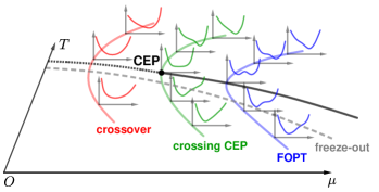
Figure 1: Schematic evolution of the Landau thermodynamical potential as a function of order parameter along the physical trajectory: with crossover (red), crossing CEP (green) and with FOPT (blue).

Considering the general phase transition theory, one may recall that the evolution of the Landau thermodynamic potential in terms of the order parameter is distinct along the process crossing the FOPT or crossover as depicted in the schematic diagram in Fig. 1. For the trajectory with a crossover, the Landau potential has only one minimum as a function of the order parameter, that gradually shifts as the temperature and chemical potential changes. For a FOPT, the thermodynamical potential shows a behavior with two local minima, and the state (phase) jumps from one minimum to another during the phase transition. Note that the potential is always continuous as a function of the order parameter. Such a picture may also explain the validity of the multiplicity distribution for the FOPT Bzdak and Koch (2019); Koch et al. (2021). The potential is in some sense a holistic observable for the phase transition, and if the system experiences the CEP or FOPT during the collision, the phase transition will leave marks on the potential even down to the freeze-out point. In this work we then propose novelly a method to construct the thermodynamical potential from the experimentally observed baryon fluctuations at different collision energies.

Constructing the thermodynamical potential from the fluctuations— The Landau thermodynamical potential is generally a Taylor expansion in terms of the order parameter. There are various choices for the order parameter that can describe the chiral phase transition of QCD. Here to associate with the experimental observables directly, we take the baryon number density as the order parameter since it is distinct in the chiral symmetric phase and the chiral symmetry broken phase and is capable of describing the order of phase transition McLerran (1987); Xin et al. (2014a). The Landau thermodynamical potential can be directly written as:

$$\Phi[n_{B}]=\sum_{k}\frac{1}{k!}\alpha_{k}\left(n_{B}-\bar{n}\right)^{k}\,,$$ (1)

where the coefficient $\alpha_{k}=\frac{\partial^{k}\Phi}{\partial n_{B}^{k}}\big{|}_{n_{B}=\bar{n}}$ is the $k$-th order Taylor coefficient at a “virtual” number density $(n_{B}-\bar{n})$ with the physical number density $\bar{n}$ at given $(T,\bar{\mu})$. The Landau potential can be related to the pressure by the Legendre transformation as $\Phi[n_{B}]\equiv n_{B}[\mu_{B}](\mu_{B}-\bar{\mu})-P[\mu_{B}]$, where $\mu_{B}$ is the conjugate variable of the $n_{B}$ of the system, $P$ is the pressure. At the physical point one has $\mu_{B}=\bar{\mu}$, $n_{B}[\bar{\mu}]=\bar{n}$ and $\Phi[\bar{n}]=-P[\bar{\mu}]$. The potential’s derivatives to $n_{B}$ can be expressed by the fluctuations order by order as:

$$\alpha_{k}\!=\!\frac{\partial\alpha_{k-1}}{\partial n_{B}}\Big{|}_{n_{B}=\bar{n}_{0}}\!\!=\!\frac{1}{C_{2}}\frac{\partial\alpha_{k-1}\left[C_{1},\cdots,C_{k-1};\mu_{B}\right]}{\partial({\mu_{B}}/T)}\Big{|}_{\mu_{B}=\bar{\mu}},$$ (2)

$$\alpha_{1}=(\mu_{B}-\bar{\mu})\big{|}_{\mu_{B}=\bar{\mu}}=0,$$ (3)

with $C_{1}=\bar{n}$ and $C_{2}=\partial n_{B}/\partial(\mu_{B}/T)$, and in general the $k$-th order susceptibility $C_{k}$ reads:

$$C_{k}=\frac{1}{T}\frac{\partial^{k}P}{\partial({\mu_{B}}/T)^{k}}\,.$$ (4)

Since it is the order of the phase transition to be concerned here rather than the exact values, we would like to redefine the potential with the dimensionless density order parameter $\tilde{n}={n_{B}}/\bar{n}-1$ as:

$$\Omega[\tilde{n}]=\frac{\Phi[n_{B}]}{T\bar{n}}=\sum_{k=2}^{\infty}\omega_{k}\frac{\tilde{n}^{k}}{k!}\,,$$ (5)

with dimensionless Taylor coefficients:

$$\omega_{2}=\frac{1}{R_{21}},\quad\quad\omega_{3}=-\frac{R_{32}}{\,R_{21}^{2}},\qquad\omega_{4}=\frac{3\,R_{32}^{2}-R_{42}}{\,R_{21}^{3}},\quad\;\;$$

$$\omega_{5}=-\frac{15\,R_{32}^{3}-10R_{42}R_{32}+R_{52}}{\,R_{21}^{4}},\qquad\qquad\qquad\qquad\qquad$$ (6)

$$\omega_{6}=\frac{105\,R_{32}^{4}-105R_{42}R_{32}^{\,2}+10R_{42}^{2}+15R_{52}R_{32}-R_{62}}{\,R_{21}^{5}},\;\;\cdots\,,\;\;$$

where we have taken $R_{ij}\equiv C_{i}/C_{j}$. Therefore, the Landau potential can be determined completely by the observables of RHIC experiments. Now if the Landau potential is capable of describing the FOPT, its Taylor expansion is required to be at least with 4-th order $\omega_{4}$, and the monotonicity of the potential determines whether a FOPT happens. The Landau potential is a monotonous function above (or below) the physical solution for the entire process of a crossover, while for the FOPT, the coexistence of two phases exhibits that one local minimum degenerates with the physical one, and a saddle point in the potential reveals the end-point of the coexistence region of the FOPT or the occurrence of the CEP. Especially if one considers the fluctuations at the freeze-out point, it is in the hadron phase with a lower number density. Therefore, one can set the criterion with having experienced a FOPT or passed through a CEP as that for $\tilde{n}\geq 0$, there exists a region with:

$$\frac{\partial\Omega[\tilde{n}]}{\partial\tilde{n}}\leq 0\,.$$ (7)

Now since the potential is a $k$-th order polynomial with a minimum at $\tilde{n}=0$, which implies:

$$\frac{\partial\Omega[\tilde{n}]}{\partial\tilde{n}}=\tilde{n}\left(\frac{\omega_{2}}{1!}+\frac{\omega_{3}}{2!}\tilde{n}+\frac{\omega_{4}}{3!}\tilde{n}^{2}+\cdots\right),$$

and the criterion of Eq. (7) is therefore related to the discriminant $\Delta$ of the $(k-2)$-th order real coefficients polynomial $\varphi[\tilde{n}]$ after eliminating the root at $\tilde{n}=0$ from $\Omega[\tilde{n}]$ which can be denoted as:

$$\varphi[\tilde{n}]=\frac{1}{\tilde{n}}\frac{\partial\Omega[\tilde{n}]}{\partial\tilde{n}}=\sum_{k=0}^{\infty}\omega_{k+2}\frac{\tilde{n}^{k}}{(k+1)!}\,.$$ (8)

The discriminant $\Delta$ of $\varphi[\tilde{n}]$ is the determinant of the Sylvester matrix with $\varphi[\tilde{n}]$ and the first order derivative of $\varphi[\tilde{n}]$ up to a common factor Gel’fand et al. (1994). For the potential up to $O(\tilde{n}^{4})$, the criterion is simple as it is the discriminant of the quadratic polynomial as:

$$\Delta=\frac{1}{4}\omega_{3}^{2}-\frac{2}{3}\omega_{2}\omega_{4}\geq 0,$$ (9)

in terms of the Taylor coefficients $\omega_{k}$. One requires $\Delta\geq 0$ so that the potential contains two more extreme points besides the physical state at $\tilde{n}=0$, one minimum for the meta-stable state and one maximum in between, which is then the feature of a FOPT. The equality $\Delta=0$ is reached at the end-point of the FOPT for the two roots becoming degenerate or at the CEP for three roots becoming degenerate, where one may further require the second derivative of the potential to be vanishing. Note that the coefficient of the highest order should be positive for a stable system, as here, $\omega_{4}>0$. A negative $\omega_{4}$ means the higher order fluctuations are required.

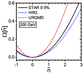
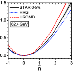
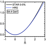
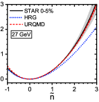
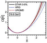
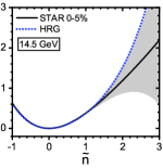
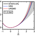
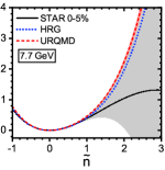
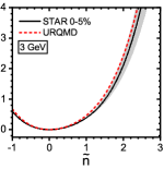
Figure 2: (colored online) The obtained thermodynamical potential up to $O(\tilde{n}^{4})$ from the STAR data of the 0-5% centrality at $\sqrt{s_{\textrm{NN}}}=200$, 62.4, 54.4, 39, 27, 19.6, 14.5, 11.5, 7.7 and 3 GeV Adam et al. (2021); Abdallah et al. (2022) (the shadow area indicates the uncertainty range), and those from theoretical calculations with the HRG Braun-Munzinger et al. (2021) and UrQMD Abdallah et al. (2021).

One can also rewrite this criterion in the form of cumulant ratios:

$$\Delta=\frac{8R_{42}-21R_{32}^{2}}{12R_{21}^{4}}\equiv\frac{8\kappa\sigma^{2}-21(S\sigma)^{2}}{12(\sigma^{2}/M)^{4}}\geq 0,$$ (10)

where $M$, $\sigma^{2}$, $S$, and $\kappa$ are the mean value, variance, skewness and kurtosis, respectively. The cumulant criterion in Eq. (10) shows that for a FOPT, the high-order cumulant $C_{4}$ should be sufficiently larger than the lower-order ones (here they are $C_{3}$ and $C_{2}$), which is in agreement with the theoretical prediction on the critical scaling Stephanov (2009, 2011) and also verified by the observed skewness and kurtosis in Ref. Adam et al. (2021). With the criterion, one may extract the possible signal of the CEP and the FOPT from the experimental observables. It also needs to mention that the criterion from the discriminant is stronger than the criterion in Eq. (7), as Eq. (7) only requires the existence of one maximum. However, if there is no other minimum, Eq. (7) will make the potential approach to negative infinity which leads to an unstable system.

For the potential up to $O(\tilde{n}^{6})$, one can also take the respective discriminant as the criterion. The detailed formula can be found in the supplemental material. For much higher order polynomials, the discriminant is only a necessary condition for FOPT and no simple relation for the criterion, but one can always check numerically if the criterion in Eq.(7) is satisfied. The general discussions of the discriminant and its relation with FOPT are also put in supplemental material.

Landau Potential with Experimental Data — As the experiments have now reached the measurements till 4-th order fluctuations in the centrality of 0-5% in a wide range of collision energy from $200$ GeV down to $3$ GeV Adam et al. (2021); Abdallah et al. (2021, 2022), the Landau potential in Eq. (5) is thus capable of being constructed directly from the data. The obtained results are illustrated in Fig. 2.

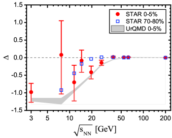
Figure 3: (colored online) The criterion $\Delta$ for the FOPT from Eq. (10) with $0$-$5\%$ centrality collisions at $\sqrt{s_{\mathrm{NN}}}=200$, $62.4$, $54.4$, $39$, $27$, $19.6$, $14.5$, $11.5$, $7.7$ and 3 GeV. The collision process has experienced a FOPT if $\Delta>0$. For high energy, the potential becomes quadratic and $\Delta$ is infinitesimal because the number density is no longer efficient as the order parameter. The results for fluctuations with $70$-$80\%$ centrality are also depicted together with the results with UrQMD computation.

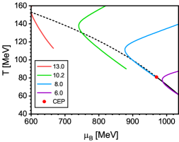
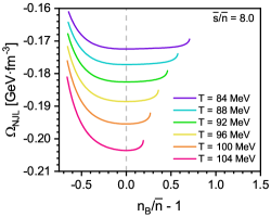
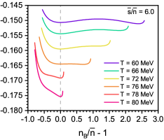
Figure 4: (colored online) Calculated phase diagram and several isentropic trajectories (labelled with the $\bar{s}/\bar{n}$ values) with crossover or FOPT via the NJL model (left panel), and the parameter dependence of the potential $\Omega_{\textrm{NJL}}$ on the baryon density (order parameter) $n$ (rescaled by the physical one $\bar{n}=n[M_{\textrm{phy.}}]$ ) at given $(T,\mu_{B})$ along two typical trajectories of crossover ($\bar{s}/\bar{n}=8.0$) and FOPT ($\bar{s}/\bar{n}=6.0$) (middle and right panels). The $(T,\mu_{B})$ position on each trajectory is controlled by the temperature.

As shown in Fig. 2, it is found that the data yield a one minimum (or monotonous in the region $\tilde{n}>0$) potential for $\sqrt{s_{\mathrm{NN}}}\geq 11.5$ GeV and thus a smooth crossover phase transition. Now it is interesting that at $\sqrt{s_{\mathrm{NN}}}=7.7$ GeV the potential changes its monotonicity in the region of $\tilde{n}>0$, which indicates that the corresponding trajectory may has crossed the phase boundary with a FOPT. However, due to the large statistical error in the experimental data, this non-monotonicity is still not robust and requires further experiments to confirm.

It is however slightly surprising that at $\sqrt{s_{\mathrm{NN}}}=3$ GeV, the signature of FOPT disappears. One possible reason is that the freeze-out point in the case of 3 GeV is too far away from the phase transition line(s) so that the possible FOPT signature is wiped out, or even the collision starts below the phase transition line.

One can also demonstrate the criterion in Eq. (10) as in Fig. 3. For $\sqrt{s_{\mathrm{NN}}}>39$ GeV, the discriminant is close to zero because the potential is mostly quadratic with $R_{21}$ being dominant. There in general does not exist another extreme point of the potential for these collision energies as shown in Fig. 2. Note that at $\sqrt{s_{\mathrm{NN}}}=39$ GeV, the value of the discriminant is slightly larger than zero, which is mainly due to the error of the measurement for the third and fourth order fluctuations and also the missing of higher order fluctuations. Moreover, the quadratic behavior of the potential also indicates that at large collision energy, the number density is no longer efficient as the order parameter since it becomes indistinguishable for the two phases.

For lower collision energy, the potential becomes quartic and enables the possibility of a FOPT. At $\sqrt{s_{\mathrm{NN}}}=14.5$ GeV, only the upper bound exceeds zero which respects the lower bound in the potential in Fig. 2. Now one may look into the potential at $\sqrt{s_{\mathrm{NN}}}=7.7$ GeV. Though there is still large uncertainty as the error of the data is large, the mean value of the experimental data clearly satisfies the criterion. This is consistent with the previous finding from Fig. 2. It also shows the sensitivity of the criterion, which makes it possible to reveal the signal of FOPT when equipping with the higher precision data. Note that the error of $C_{4}$ is dominant in the error band of the potential, and hence, it is essential to improve the measurement of $C_{4}$ in comparison to the other fluctuations.

Besides, the cumulant ratios from some theoretical calculations are also incorporated in Fig. 2 and  3, including those with the hadron resonance gas (HRG) model Braun-Munzinger et al. (2021) and the UrQMD transport model Bleicher et al. (1999). We verify that the potential constructed from the fluctuations of the HRG and UrQMD always give a monotonous behavior in the $\tilde{n}>0$ region with also the discriminant always being negative, which is consistent with the fact that there is no FOPT in these approaches. The results for larger centrality in the $70-80\%$ regions are also shown in Fig. 3. The criterion for FOPT is not satisfied for all energies in case of such a centrality collisions. Incorporating with the theoretical methods like DSE and fRG which have predicted the existence of the CEP may be able to give a proper estimation at which collision energy the FOPT can be observed from the fluctuations Isserstedt et al. (2019); Fu et al. (2021); Gao and Pawlowski (2022), and the work is under progress.

An illustration with effective model calculation— To verify the above results obtained from general analysis and experimental data, we illustrate the complete evolution procedure of the thermodynamic potential during the physical process, which is obtained with the simple Nambu–Jona-Lasinio (NJL) model Buballa (2005). For a degenerate $N_{f}$ flavor system, the potential in the NJL model reads:

$$\frac{\Omega_{\textrm{NJL}}[M]}{V}=\frac{(M-m_{0})^{2}}{4G}-2N_{c}N_{f}\int_{0}^{\Lambda}\frac{d^{3}\bm{p}}{(2\pi)^{3}}\bigg{\{}E_{\bm{p}}\qquad\quad$$

$$\;+T\,\log\left[1\!+e^{-(E_{\bm{p}}-\mu)/T}\right]+T\,\log\left[1\!+e^{-(E_{\bm{p}}+\mu)/T}\right]\bigg{\}},$$ (11)

where $M$ is the mean-field constituent quark mass which is also a typical order parameter of the chiral phase transition, $m_{0}$ is the current quark mass, $\mu={\mu_{B}}/3$ is the degenerate quark chemical potential, $E_{\bm{p}}=\sqrt{\bm{p}^{2}+M^{2}}$ and $\Lambda$ the momentum cut-off of the model.

The physical state corresponding to the potential are determined by the gap equation $\delta\Omega/\delta M=0$, which reads explicitly as

$$M {}^{\textrm{phy.}}=m_{0}+N_{c}N_{f}\,GM^{\textrm{phy.}}\int_{0}^{\Lambda}\frac{p^{2}\,dp}{\pi^{2}\,E_{p}^{\textrm{phy.}}}$$

$$\times\left[\tanh\left(\frac{E_{p}^{\textrm{phy.}}-\mu}{2T}\right)+\tanh\left(\frac{E_{p}^{\textrm{phy.}}+\mu}{2T}\right)\right].$$ (12)

For a stable state, the additional condition $\delta^{2}\Omega/\delta M^{2}>0$ is also implemented so that it locates at a local minimum of the potential.

The phase diagram can be then calculated. For the FOPT, the phase transition boundary is determined with the criterion that the potential of the Nambu phase is equal to that of the Wigner phase Jiang et al. (2013); Xin et al. (2014b), $\Omega[M_{N}]=\Omega[M_{W}]$. For the crossover, the phase boundary is determined by the maximum of the chiral susceptibility $\chi_{T}=\partial M/\partial T$. We consider the case with $N_{f}=2$ light flavors and implement the model parameters: $m_{0}=5.6$ MeV, $\Lambda=587.9$ MeV and $G\Lambda^{2}=2.44$.

We then consider the isentropic trajectories with $\bar{s}/\bar{n}=constant$ as the physical evolution trajectories. $\bar{s}$ and $\bar{n}$ are the entropy and the baryon density at the physical point with $M=M^{\textrm{phy.}}$, and as usual, the entropy $s$ and number density $n_{B}$ is determined from the potential in Eq. (11) as

$$s[M;T,\mu_{B}] \displaystyle=-\left(\frac{\partial\,\Omega[M;T,\mu_{B}]}{\partial\,T}\right)_{M,T},$$ (13)

$$n_{B}[M;T,\mu_{B}] \displaystyle=-\left(\frac{\partial\,\Omega[M;T,\mu_{B}]}{\partial\,\mu_{B}}\right)_{M,T}.$$ (14)

The obtained results of the phase diagram and several isentropic trajectories are shown in Fig. 4.

It is now interesting to look through the evolution of the thermodynamical potential along the trajectories. If regarding the mass $M$ as the order parameter, which has been studied widely (e.g. Refs. Buballa (2005); Xin et al. (2014b)), one found that the evolution behavior is closely related to the QCD phase structure. Since we are interested in the virtual baryon density dependence which is related to the cumulants ratios, we convert the original order parameter $M$ to baryon density $n[M]$ by the relation in Eq. (14), which satisfies $\bar{n}=n[M_{\textrm{phy.}}]$ at the physical point.

The parameter dependence of $\Omega[n_{B}]$ is computed along each certain trajectory in a temperature range $T-T_{c}\in(-15,+5)$ MeV with $T_{c}$ the critical one at which the trajectory intersects with the phase boundary. Here we pick two benchmarks $\bar{s}/\bar{n}=6.0$, 8.0 for the FOPT, the crossover, respectively. The results are also shown in Fig. 4. It is found evidently that, within such a range of $\;T-T_{c}$, the $\Omega[n_{B}]$ in case of the FOPT is in general non-convex and non-monotonous near the phase boundary, whereas in the crossover region, e.g., the case with $\bar{s}/\bar{n}=8.0$, the $\Omega[n_{B}]$ is always convex even if the trajectory may travel very close to the CEP. In short, the thermodynamical potential is distinct from each other in the cases of the crossover and the FOPT. Such a feature maintains at least within the temperature range $T-T_{c}\in(-15,+5)$ MeV along the trajectories, so that it is possible to survive in the experimental measurement Fu et al. (2020); Gao and Pawlowski (2020).

Summary— The thermodynamical potential opens an access to track the physical process in the heavy-ion collision, and thus makes it possible to probe the signal of the CEP or FOPT even it occurs at the freeze-out point, which is away from the phase boundary. The criterion from the potential is more general and powerful than that from the fluctuation itself because of the synergy that the potential assembles all orders of the fluctuations to the verdict of the signal of phase transition. Especially, if the potential can be constructed in a model-independent way, it would be greatly helpful to search for the phase transition experimentally. Therefore, We proposed a novel method to construct the potential directly through the experimental data in this Letter. With the net-proton fluctuations measured in Au+Au collisions at $\sqrt{s_{\mathrm{NN}}}$ = 3–200 GeV by the STAR experiment, we obtain the Landau potential at each energy and the energy dependence of the criterion for the FOPT. It is found that the criterion derived from the fluctuations from the peripheral (70-80%) Au+Au collisions and UrQMD model are negative and show monotonic decreasing as a function of energy, indicating no signal of FOPT. Further, the criterion are negative for almost all the energies with the 0-5% most central data and consistent with the results from UrQMD with large uncertainties. An exception is that, at $\sqrt{s_{\mathrm{NN}}}=7.7$ GeV, the mean value of the current data satisfies the criterion of FOPT. However, the uncertainties of the experimental measurement are still too large to give a conclusive assertion. Besides, though the quadratic potential is already enough for describing the FOPT, the higher order fluctuations can help to confirm the convergence of the Taylor expansion. In all, a high precision measurement of the $C_{1,...,6}$ in 0-5% centrality in the neighborhood of $\sqrt{s_{\mathrm{NN}}}=7.7$ GeV is of primary importance to finally verify the FOPT of QCD.

I Ackowledgement

The authors thank the fQCD collaboration fQCD collaboration (2022) for fruitful discussions. YL and YXL was supported by the National Natural Science Foundation of China (NSFC) under Grant Nos. 11175004 and 12175007. XL was supported by the National Key Research and Development Program of China with grant Nos. 2022YFA1605501, 2020YFE0202002 and 2018YFE0205201, the NSFC with grant Nos. 12122505 and 11890711) and the Fundamental Research Funds of the Central China Normal University with grant No. CCNU220N003. LC was supported by the NSFC with Grant No. 12135007.

II Supplemental material: The criterion of CEP and FOPT and the discriminant of the polynomial

Considering the criterion function $\varphi[x]$ as a general $n$-th order polynomial of argument $x$ as:

$$\varphi[x]=a_{n}x^{n}+\cdots+a_{0},$$ (15)

with $\displaystyle a_{n}=\frac{\omega_{n+2}}{(n+1)!}$, which is a polynomial with two degrees lower than the potential $\Omega$ (as defined in Eq. (8)). If the potential describes the FOPT, it must have two minima and one maximum. One minimum is the physical state and the other minimum is the meta-stable state. Therefore, $\varphi[x]$ should contain two real roots since the root for physical state has been eliminated. The property of the roots is in general related to its discriminant $\Delta$ which is defined as:

$$\Delta=(-1)^{\frac{1}{2}n(n-1)}\frac{1}{a_{n}}R$$ (16)

with $R$ the determinant of its respective $(2n-1)\times(2n-1)$ Sylvester matrix as:

$$\begin{gathered}\begin{bmatrix}a_{n}&a_{n-1}&a_{n-2}&\cdots&a_{1}&a_{0}&0&\cdots&0\\[2.84526pt] 0&a_{n}&a_{n-1}&a_{n-2}&\cdots&a_{1}&a_{0}&\cdots&0\\[2.84526pt] \vdots&\vdots&\vdots&\vdots&\vdots&\vdots&\vdots&\vdots&\vdots\\[2.84526pt] 0&0&0&a_{n}&a_{n-1}&a_{n-2}&\cdots&\cdots&a_{0}&\\[2.84526pt] na_{n}&(n-1)a_{n-1}&(n-2)a_{n-2}&\cdots&a_{1}&0&\cdots&\cdots&0\\[2.84526pt] 0&na_{n}&(n-1)a_{n-1}&(n-2)a_{n-2}&\cdots&a_{1}&\cdots&0&0\\[2.84526pt] \vdots&\vdots&\vdots&\vdots&\vdots&\vdots&\vdots&\vdots&\vdots\\[2.84526pt] 0&0&\cdots&0&na_{n}&(n-1)a_{n-1}&\cdots&\cdots&a_{1}&\\ \end{bmatrix}\end{gathered}$$ (17)

Generally speaking, for $n$-th order polynomials, one requires two real roots in $\varphi[x]$ to describe the feature of a FOPT, and the surplus roots should be complex in order to avoid more minima in the potential which are not physical. Now for polynomials with real coefficients as considered here, the complex roots can only exist in pairs and moreover, there exist even-number pairs of complex roots with the discriminant $\Delta>0$, while exist odd-number pairs for $\Delta<0$. Therefore, for an odd-order potential, the related $\varphi[x]$ then has an odd number of real roots, rather than two. Also, despite the fact that Eq. (7) can be satisfied in this case, the potential is unstable for an infinitely large density as it diverges to negative infinity. The order of $\varphi[x]$ should be even to guarantee that it has exactly two real roots. For the case of order $2(2m+1)$, one entails $\Delta>0$ which brings in even-number pairs of complex roots and thus satisfies the requirement of containing two real roots, while for order $2(2m)$, one then entails $\Delta<0$. Note that the discriminant does not constrain completely the number of the roots, the detailed technique is beyond the scope of this work and here we simply apply the discriminant as the criterion which completely constrains the polynomials to have two real roots in the quadratic and quartic cases.

For a fourth order potential, $\varphi[x]$ is a quadratic polynomial and thus one has the criterion for having CEP and FOPT as:

$$\Delta=a_{1}^{2}-4a_{2}a_{0}=\frac{1}{4}\omega_{3}^{2}-\frac{2}{3}\omega_{2}\omega_{4}\geq 0\,,$$ (18)

which is just the criterion in Eq. (9).

For sixth order potential, the discriminant is lengthy. We simply put the criterion in $a_{k}$ here as:

$$\Delta = a_{1}^{2}a_{2}^{2}a_{3}^{2}-4a_{0}a_{2}^{3}a_{3}^{2}-4a_{1}^{3}a_{3}^{3}+18a_{0}a_{1}a_{2}a_{3}^{3}$$ (19)

$$-27a_{0}^{2}a_{3}^{4}-4a_{1}^{2}a_{2}^{3}a_{4}+16a_{0}a_{2}^{4}a_{4}+18a_{1}^{3}a_{2}a_{3}a_{4}$$

$$-80a_{0}a_{1}a_{2}^{2}a_{3}a_{4}-6a_{0}a_{1}^{2}a_{3}^{2}a_{4}+144a_{0}^{2}a_{2}a_{3}^{2}a_{4}$$

$$-27a_{1}^{4}a_{4}^{2}+144a_{0}a_{1}^{2}a_{2}a_{4}^{2}-128a_{0}^{2}a_{2}^{2}a_{4}^{2}$$

$$-192a_{0}^{2}a_{1}a_{3}a_{4}^{2}+256a_{0}^{3}a_{4}^{3}\leq 0\,.$$

When $\omega_{5}$ and $\omega_{6}$ are small, the above criterion in Eq. (19) degenerates into Eq. (18).

References

- Council (2013) N. R. Council, Nuclear Physics: Exploring the Heart of Matter (The National Academies Press, Washington, DC, 2013).
- Aoki et al. (2006) Y. Aoki, G. Endrődi, Z. Fodor, et al., Nature 443, 675 (2006).
- Aoki et al. (2009) Y. Aoki, S. Borsányi, S. Dürr, et al., J. High Energy Phys. 2009, 088 (2009).
- Borsányi et al. (2010) S. Borsányi, Z. Fodor, C. Hoelbling, et al., J. High Energy Phys. 2010 (2010).
- Bazavov et al. (2012) A. Bazavov et al. (HotQCD Collaboration), Phys. Rev. D 85, 054503 (2012).
- Bonati et al. (2018) C. Bonati, M. D’Elia, F. Negro, et al., Phys. Rev. D 98, 054510 (2018).
- Bazavov et al. (2019) A. Bazavov et al. (HotQCD Collaboration), Phys. Lett. B 795, 15 (2019).
- Borsanyi et al. (2020) S. Borsanyi, Z. Fodor, J. N. Guenther, et al., Phys. Rev. Lett. 125, 052001 (2020).
- Asakawa and Yazaki (1989) M. Asakawa and K. Yazaki, Nucl. Phys. A 504, 668 (1989).
- Klevansky (1992) S. P. Klevansky, Rev. Mod. Phys. 64, 649 (1992).
- Barducci et al. (1994) A. Barducci, R. Casalbuoni, G. Pettini, et al., Phys. Rev. D 49, 426 (1994).
- Stephanov (1996) M. A. Stephanov, Phys. Rev. Lett. 76, 4472 (1996).
- Alford et al. (1998) M. Alford, K. Rajagopal, and F. Wilczek, Phys. Lett. B 422, 247 (1998).
- Rapp et al. (1998) R. Rapp, T. Schäfer, E. Shuryak, et al., Phys. Rev. Lett. 81, 53 (1998).
- Berges and Rajagopal (1999) J. Berges and K. Rajagopal, Nucl. Phys. B 538, 215 (1999).
- Fischer et al. (2014) C. S. Fischer, J. Luecker, and C. A. Welzbacher, Phys. Rev. D 90, 034022 (2014).
- Gao and Liu (2016) F. Gao and Y.-x. Liu, Phys. Rev. D 94, 076009 (2016).
- Gunkel and Fischer (2021) P. J. Gunkel and C. S. Fischer, Phys. Rev. D 104, 054022 (2021).
- Lu et al. (2022) Y. Lu, M.-y. Chen, Z. Bai, et al., Phys. Rev. D 105, 034012 (2022).
- Fu et al. (2020) W.-j. Fu, J. M. Pawlowski, and F. Rennecke, Phys. Rev. D 101, 054032 (2020).
- Gao and Pawlowski (2020) F. Gao and J. M. Pawlowski, Phys. Rev. D 102, 034027 (2020).
- Gao and Pawlowski (2021) F. Gao and J. M. Pawlowski, Phys. Lett. B 820, 136584 (2021).
- Abelev et al. (2010) B. I. Abelev et al. (STAR Collaboration), Phys. Rev. C 81, 024911 (2010).
- Mohanty (2009) B. Mohanty, Nucl. Phys. A 830, 899c (2009).
- Gupta et al. (2011) S. Gupta, X.-f. Luo, B. Mohanty, et al., Science 332, 1525 (2011).
- Luo and Xu (2017) X.-f. Luo and N. Xu, Nucl. Sci. Tech. 28, 112 (2017).
- Stephanov et al. (1999) M. Stephanov, K. Rajagopal, and E. Shuryak, Phys. Rev. D 60, 114028 (1999).
- Asakawa et al. (2000) M. Asakawa, U. Heinz, and B. Müller, Phys. Rev. Lett. 85, 2072 (2000).
- Hatta and Ikeda (2003) Y. Hatta and T. Ikeda, Phys. Rev. D 67, 014028 (2003).
- Stephanov (2009) M. A. Stephanov, Phys. Rev. Lett. 102, 032301 (2009).
- Stephanov (2011) M. A. Stephanov, Phys. Rev. Lett. 107, 052301 (2011).
- Luo (2015) X. Luo, J. Phys.: Conf. Ser. 599, 012023 (2015).
- Asakawa and Kitazawa (2016) M. Asakawa and M. Kitazawa, Prog. Part. Nucl. Phys. 90, 299 (2016).
- Bzdak and Koch (2019) A. Bzdak and V. Koch, Phys. Rev. C 100, 051902 (2019).
- Koch et al. (2021) V. Koch, A. Bzdak, D. Oliinychenko, et al., Nucl. Phys. A 1005, 121968 (2021).
- McLerran (1987) L. D. McLerran, Phys. Rev. D 36, 3291 (1987).
- Xin et al. (2014a) X.-y. Xin, S.-x. Qin, and Y.-x. Liu, Phys. Rev. D 90, 076006 (2014a).
- Gel’fand et al. (1994) I. Gel’fand, M. Kapranov, and A. Zelevinsky, Discriminants, Resultants, and Multidimensional Determinants, Mathematics (Birkhäuser) (Springer, 1994).
- Adam et al. (2021) J. Adam et al. (STAR Collaboration), Phys. Rev. Lett. 126, 092301 (2021).
- Abdallah et al. (2022) M. S. Abdallah et al. (STAR Collaboration), Phys. Rev. Lett. 128, 202303 (2022).
- Braun-Munzinger et al. (2021) P. Braun-Munzinger, B. Friman, K. Redlich, et al., Nucl. Phys. A 1008, 122141 (2021).
- Abdallah et al. (2021) M. S. Abdallah et al. (STAR Collaboration), Phys. Rev. C 104, 024902 (2021).
- Bleicher et al. (1999) M. Bleicher, E. Zabrodin, C. Spieles, et al., J. Phys. G: Nucl. Part. Phys. 25, 1859 (1999).
- Isserstedt et al. (2019) P. Isserstedt, M. Buballa, C. S. Fischer, et al., Phys. Rev. D 100, 074011 (2019).
- Fu et al. (2021) W.-j. Fu, X.-f. Luo, J. M. Pawlowski, et al., Phys. Rev. D 104, 094047 (2021).
- Gao and Pawlowski (2022) F. Gao and J. M. Pawlowski, Phys. Rev. D 105, 094020 (2022).
- Buballa (2005) M. Buballa, Phys. Rep. 407, 205 (2005).
- Jiang et al. (2013) L.-j. Jiang, X.-y. Xin, K.-l. Wang, et al., Phys. Rev. D 88, 016008 (2013).
- Xin et al. (2014b) X.-y. Xin, S.-x. Qin, and Y.-x. Liu, Phys. Rev. D 89, 094012 (2014b).
- fQCD collaboration (2022) fQCD collaboration, (2022), J. Braun, Y.-r. Chen, W.-j. Fu, F. Gao, F. Ihssen, A. Geissel, J. Horak, C. Huang, J. M. Pawlowski, F. Rennecke, F. Sattler, B. Schallmo, C. Schneider, Y.-y. Tan, S. Töpfel, R. Wen, J. Wessely, N. Wink and S. Yin.