Ruling Out Primordial Black Hole Formation From Single-Field Inflation

Abstract

The most widely studied formation mechanism of a primordial black hole (PBH) is collapse of large-amplitude perturbation on small scales generated in single-field inflation. In this Letter, we calculate one-loop correction to the large-scale power spectrum in such a model. We find models producing appreciable amount of PBHs induce nonperturbative coupling on large scale probed by cosmic microwave background radiation. We therefore conclude that PBH formation from cosmological perturbation theory in single-field inflation is ruled out.

Primordial black holes (PBHs) have been a research interest for more than 50 years [1, 2, 3], although there has been no observational evidence for them. They could be light enough for Hawking radiation to be important [4], they are a potential dark matter candidate [5, 6, 7, 8, 9, 10, 11, 12, 13, 14] (reviewed in [15, 16]), and they can explain LIGO-Virgo gravitational wave events [17, 18, 19, 20, 21, 22].

A number of formation mechanisms of PBHs in the early Universe has been proposed. The most well-studied one makes use of quantum fluctuations [23, 24, 25, 26] generated in cosmic inflation [27, 28, 29]. Observations of CMB anisotropy [30, 31, 32] tightly constrain these fluctuations on large scales. Their power spectrum is almost scale invariant with the amplitude $2.1\times 10^{-9}$. On smaller scales that cannot be probed by CMB observations, observational constraints are loose enough [33, 34, 35, 36, 37, 38, 39]. Therefore, it is possible to have a theory which produce large fluctuations with the amplitude of power spectrum $\mathcal{O}(0.01)$ that satisfy observational constraints and many models have been proposed to realize such a feature [7, 40, 8, 41, 42, 43, 44, 45, 46, 47, 48, 49, 50, 51, 52, 53, 54, 55, 56, 57, 58, 59, 60, 61, 62, 63, 64, 65, 66, 67, 68, 69, 70, 71, 72, 73, 74, 75, 76, 77, 78, 79, 80, 81, 82, 83, 84, 85, 86, 87, 88, 89, 90, 91, 92, 93]. Peaks of such fluctuations may collapse into PBHs with appreciable abundance [94, 95] after entering the horizon, which also produce large stochastic gravitational wave background [96, 97, 98, 99, 100] that can be probed by future gravitational wave observations as well as pulsar timing array experiments [101].

The simplest inflation model that is consistent with current observational data [31, 32] is canonical slow-roll (SR) inflation as reviewed in [102]. It is described by a scalar field $\phi$, called inflaton, with a canonical kinetic term and potential $V(\phi)$ in quasi-de Sitter space. The standard SR inflation generates nearly scale-invariant adiabatic curvature perturbation that behaves classically as the decaying mode decreases exponentially during inflation, so that the perturbation variable and its conjugate momentum practically commute with each other [103]. In order to be consistent with CMB observations [31, 32], the shape of the potential is tightly constrained for a finite range of $\phi$.

If the inflaton passes through an extremely flat region of the potential with $\mathrm{d}V/\mathrm{d}\phi\approx 0$ after the comoving scales probed by CMB have left the horizon, it may produce large-amplitude fluctuations on small scales. In this region, slow-roll condition fails, and the inflation goes into a temporary ultraslow-roll (USR) period [104, 105, 106, 107, 108]. During this regime the non-constant mode of fluctuations, which would decay exponentially in SR inflation, actually grows, as observed in other models [109, 81], resulting in enhanced power spectrum on specific scales. This may also imply the importance of quantum effects as we will see below.

Many inflation models with a flat region or inflection point of the potential have been proposed inspired by high energy theories such as supergravity [42, 43, 44, 45, 46, 47, 48], axion monodromy [49, 50], scalaron in $R^{2}$-gravity [51], $\alpha$-attractor [52, 53, 54], and string theory [55, 56, 57], as well as in Higgs inflation which does not require theories beyond the standard model [58, 59, 60, 61, 62]. As an extension of USR period, constant-roll inflation can also produce large amplitudes [110, 75].

Theoretically, the power spectrum is described by the vacuum expectation value (VEV) of the fluctuation two-point functions in quantum field theory, to which only wavevectors with equal magnitude and opposite direction contribute. As we expand the theory to higher-order in fluctuations, we will get higher-order interaction terms, which generate primordial non-Gaussianity or VEV of the higher-point functions which are calculated by in-in perturbation theory [111, 112, 113]. At the same time, such interactions also generate back reaction to the two-point function which is called loop correction [114, 115, 116, 117, 118, 119, 120, 121, 122]. These corrections behave non-linearly, where fluctuations with different wavenumber magnitude can contribute. Therefore, small-scale fluctuations can contribute to the loop corrections of the CMB-scale fluctuation two-point functions.

As mentioned above, in order to realize PBH formation appropriately, we need an inflation model producing enhanced power spectrum with the amplitude $\mathcal{O}(0.01)$ on a certain small scale while keeping the amplitude at $2.1\times 10^{-9}$ on CMB scale. However, such a requirement is only a tree-level statement. So far, understanding of inflation models accommodating PBH formation is very limited beyond tree-level, although it has been discussed in [123, 124, 125, 126, 127, 128, 129] for some specific models. It is important to ensure that one-loop correction is suppressed compared to the tree-level contribution, so that we can still trust the perturbation theory.

In our previous papers [121, 122], we showed that one-loop perturbativity bound can strongly constrain single-field inflation models. We have also qualitatively pointed out a possible problem in PBH formation mechanism. In this Letter, we use one-loop perturbativity requirement to examine the possibility of PBH formation models in single-field inflation. We calculate contribution of the peak of power spectrum on small scale to one-loop correction of the CMB-scale power spectrum. Requiring one-loop correction to be much smaller than tree-level contribution, we obtain an upper-bound on the power spectrum on small scale.

We specifically consider a PBH formation from an extremely flat region in the potential that leads to a temporary USR motion of the inflaton. At the end, we will explain that our result can be generalized to other PBH formation models in single-field inflation.

The action of canonical inflation is given by

$$S=\frac{1}{2}\int\mathrm{d}^{4}x\sqrt{-g}\left[M_{\mathrm{pl}}^{2}R-(\partial_{\mu}\phi)^{2}-2V(\phi)\right],$$ (1)

where $M_{\mathrm{pl}}$ is reduced Planck scale, $g=\mathrm{det}~{}g_{\mu\nu}$, $g_{\mu\nu}$ and $R$ are metric tensor and its Ricci scalar. Consider a spatially flat, homogeneous and isotropic background

$$\mathrm{d}s^{2}=-\mathrm{d}t^{2}+a^{2}(t)\mathrm{d}\mathbf{x}^{2}=a^{2}(\tau)(-\mathrm{d}\tau^{2}+\mathrm{d}\mathbf{x}^{2}),$$ (2)

where $\tau$ is conformal time. Equations of motion for the scale factor $a(t)$ and the homogeneous part of the inflaton $\phi(t)$ are the Friedmann equations

$$H^{2}=\frac{1}{3M_{\mathrm{pl}}^{2}}\left(\frac{1}{2}\dot{\phi}^{2}+V(\phi)\right),~{}\dot{H}=-\frac{\dot{\phi}^{2}}{2M_{\mathrm{pl}}^{2}},$$ (3)

with $H=\dot{a}/{a}$ being the Hubble parameter, and the Klein-Gordon equation

$$\ddot{\phi}+3H\dot{\phi}+\frac{\mathrm{d}V}{\mathrm{d}\phi}=0.$$ (4)

When CMB-scale fluctuations leave the horizon at around $\phi_{\mathrm{CMB}}$ (see Fig. 1), the potential is slightly tilted to realize slow-roll inflation, satisfying

$$\absolutevalue{\frac{\ddot{\phi}}{\dot{\phi}H}}\ll 1,~{}\epsilon\equiv-\frac{\dot{H}}{H^{2}}=\frac{\dot{\phi}^{2}}{2M_{\mathrm{pl}}^{2}H^{2}}\ll 1,$$ (5)

where $\epsilon$ is a SR parameter. In the SR period, $\epsilon$ is approximately constant. Then the inflaton goes through an extremely flat region of the potential, between time $t_{s}$ to $t_{e}$, experiencing an USR period. When inflaton enters this region with $\mathrm{d}V/\mathrm{d}\phi\approx 0$, Eq. (4) becomes $\ddot{\phi}\approx-3H\dot{\phi}$, so $\dot{\phi}\propto a^{-3}$, which breaks SR approximation [107]. This makes $\epsilon$ strongly time-dependent and extremely small as

$$\epsilon=\frac{\dot{\phi}^{2}}{2M_{\mathrm{pl}}^{2}H^{2}}\propto a^{-6}.$$ (6)

We also define the second SR parameter

$$\eta\equiv\frac{\dot{\epsilon}}{\epsilon H}=2\epsilon+2\frac{\ddot{\phi}}{\dot{\phi}H},$$ (7)

which is approximately constant and very small in SR period $\eta\ll 1$, but large in USR period $\eta\approx-6$. The latter regime satisfies the condition of the growth of the non-constant mode of perturbation found in [81], namely, $3-\epsilon+\eta<0$, so that enhanced spectrum is obtained then.

After the USR period, the inflaton enters SR period again until the end of inflation. In both SR and USR period, because $\epsilon$ is very small, the scale factor can be approximated as $a=-1/H\tau\propto e^{Ht}$.

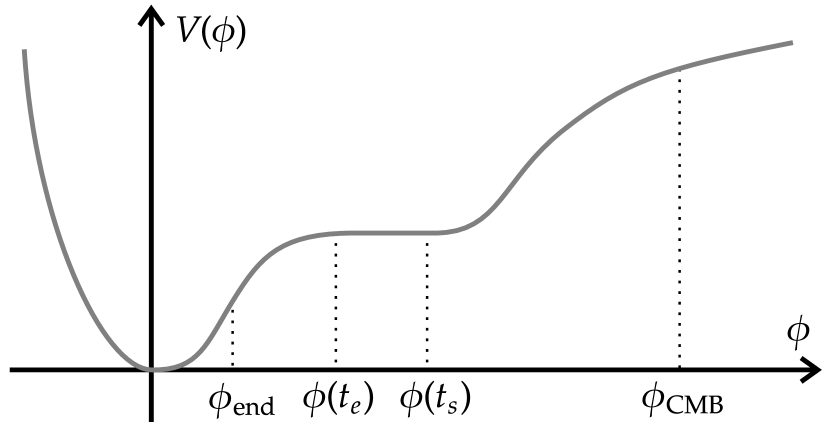
Figure 1: Schematic picture of the inflaton potential realizing PBH formation. When the inflaton is around $\phi_{\mathrm{CMB}}$, scales probed by CMB observations leave horizon and it is in the SR regime. It enters an extremely flat region at $t=t_{s}$ undergoing an USR period. It enters SR period again at $t=t_{e}$ until $\phi_{\mathrm{end}}$, the end of inflation.

Small perturbation from the homogeneous part, $\phi(t)$, of the inflaton $\phi(\mathbf{x},t)$ and metric can be expressed as

$$\phi(\mathbf{x},t)=\phi(t)+\delta\phi(\mathbf{x},t),$$

$$\mathrm{d}s^{2}=-N^{2}\mathrm{d}t^{2}+\gamma_{ij}(\mathrm{d}x^{i}+N^{i}\mathrm{d}t)(\mathrm{d}x^{j}+N^{j}\mathrm{d}t),$$ (8)

where $\gamma_{ij}$ is the three-dimensional metric on slices of constant $t$, $N$ is the lapse function, and $N^{i}$ is the shift vector. We choose comoving gauge condition

$$\delta\phi(\mathbf{x},t)=0,~{}\gamma_{ij}(\mathbf{x},t)=a^{2}(t)e^{2\zeta(\mathbf{x},t)}\delta_{ij},$$ (9)

where $\zeta(\mathbf{x},t)$ is curvature perturbation. Here, tensor perturbation is not relevant. Also, $N$ and $N^{i}$ are obtained by solving constraint equations.

Expanding the action (1) up to the second-order of the curvature perturbation yields

$$S^{(2)}=M_{\mathrm{pl}}^{2}\int\mathrm{d}t~{}\mathrm{d}^{3}x~{}a^{3}\epsilon\left[\dot{\zeta}^{2}-\frac{1}{a^{2}}(\partial_{i}\zeta)^{2}\right].$$ (10)

In terms of Mukhanov-Sasaki variable $v=zM_{\mathrm{pl}}\zeta$, where $z=a\sqrt{2\epsilon}$, the action becomes canonically normalized

$$S^{(2)}=\frac{1}{2}\int\mathrm{d}\tau~{}\mathrm{d}^{3}x\left[(v^{\prime})^{2}-(\partial_{i}v)^{2}+\frac{z^{\prime\prime}}{z}v^{2}\right],$$ (11)

where a prime denotes derivative with respect to $\tau$ [23, 130]. In momentum space, quantization is performed by promoting the Mukhanov-Sasaki variable as an operator

$$\hat{v}(\mathbf{k},\tau)=M_{\mathrm{pl}}z\zeta(\mathbf{k},\tau)=v_{k}(\tau)\hat{a}_{\mathbf{k}}+v^{*}_{k}(\tau)\hat{a}_{-\mathbf{k}}^{\dagger},$$ (12)

where mode function $v_{k}(\tau)$ approximately satisfies

$$v_{k}^{\prime\prime}+\left(k^{2}-\frac{2}{\tau^{2}}\right)v_{k}=0,$$ (13)

in both SR and USR regimes, and the operators satisfy the commutation relation $[\hat{a}_{\mathbf{k}},\hat{a}_{-\mathbf{k^{\prime}}}^{\dagger}]=(2\pi)^{3}\delta^{3}(\mathbf{k}+\mathbf{k^{\prime}})$ under the normalization condition

$$v_{k}^{\prime*}v_{k}-v_{k}^{\prime}v_{k}^{*}=i.$$ (14)

The general solution of mode function $v_{k}(\tau)$ is

$$v_{k}(\tau)=\frac{\mathcal{A}_{k}}{\sqrt{2k}}\left(1-\frac{i}{k\tau}\right)e^{-ik\tau}+\frac{\mathcal{B}_{k}}{\sqrt{2k}}\left(1+\frac{i}{k\tau}\right)e^{ik\tau},$$ (15)

where $\mathcal{A}_{k}$ and $\mathcal{B}_{k}$ are determined by boundary conditions.

At an early time, $t\lesssim t_{s}$, the inflaton was in SR period with Bunch-Davies initial vacuum, a state $\ket{0}$ defined by $\hat{a}_{\mathbf{k}}\ket{0}=0$ with $\mathcal{A}_{k}=1$ and $\mathcal{B}_{k}=0$. Mode function of the curvature perturbation $\zeta_{k}=v_{k}/zM_{\mathrm{pl}}$ is

$$\zeta_{k}(\tau)=\left(\frac{iH}{2M_{\mathrm{pl}}\sqrt{\epsilon_{\mathrm{SR}}}}\right)_{\star}\frac{e^{-ik\tau}}{k^{3/2}}(1+ik\tau),$$ (16)

where $\epsilon_{\mathrm{SR}}$ is $\epsilon$ in SR period and subscript $\star$ denotes the value at the horizon crossing epoch $\tau=-1/k$.

At $t_{s}\lesssim t\lesssim t_{e}$, the inflaton is in USR period. We define $\tau_{s}$ and $\tau_{e}$ as conformal time corresponding to $t_{s}$ and $t_{e}$, respectively. The SR parameter $\epsilon$ can be written as $\epsilon(\tau)=\epsilon_{\mathrm{SR}}(\tau/\tau_{s})^{6}$ based on proportionality in (6). Therefore, the curvature perturbation becomes

$$\zeta_{k}(\tau)= ~{}\left(\frac{iH}{2M_{\mathrm{pl}}\sqrt{\epsilon_{\mathrm{SR}}}}\right)_{\star}\left(\frac{\tau_{s}}{\tau}\right)^{3}\frac{1}{k^{3/2}}$$

$$\times\left[\mathcal{A}_{k}e^{-ik\tau}(1+ik\tau)-\mathcal{B}_{k}e^{ik\tau}(1-ik\tau)\right],$$ (17)

where coefficients $\mathcal{A}_{k}$ and $\mathcal{B}_{k}$ are determined by matching to the SR solution (16) at the boundary. We consider instantaneous transition from SR to USR, because it is a good approximation to numerical solutions [131]. Solutions of the coefficients by requiring continuity of $\zeta_{k}(\tau)$ and $\zeta_{k}^{\prime}(\tau)$ at transition $\tau=\tau_{s}$ are [132, 133, 134, 135, 136, 131, 137]

$$\mathcal{A}_{k}=1-\frac{3(1+k^{2}\tau_{s}^{2})}{2ik^{3}\tau_{s}^{3}},~{}\mathcal{B}_{k}=-\frac{3(1+ik\tau_{s})^{2}}{2ik^{3}\tau_{s}^{3}}e^{-2ik\tau_{s}}.$$ (18)

At late time, $t\gtrsim t_{e}$, the inflaton goes back to SR dynamics. We define $k_{s}$ and $k_{e}$ as wavenumbers which cross the horizon at $\tau_{s}$ and $\tau_{e}$, respectively. For perturbation with wavenumber $k\lesssim k_{e}$, the mode function approaches constant as $\zeta_{k}(\tau)\approx\zeta_{k}(\tau_{e})$. For perturbation with $k\gtrsim k_{e}$, the mode function can be approximated as (16).

The two-point functions of curvature perturbation and power spectrum at the end of inflation, $\tau_{0}~{}(\rightarrow 0)$, can be written as

$$\left\langle\zeta(\mathbf{k})\zeta(\mathbf{k^{\prime}})\right\rangle\equiv(2\pi)^{3}\delta^{3}(\mathbf{k}+\mathbf{k^{\prime}})\left\langle\!\left\langle\zeta(\mathbf{k})\zeta(-\mathbf{k})\right\rangle\!\right\rangle,$$ (19)

$$\Delta^{2}_{s}(k)\equiv\frac{k^{3}}{2\pi^{2}}\left\langle\!\left\langle\zeta(\mathbf{k})\zeta(-\mathbf{k})\right\rangle\!\right\rangle,$$ (20)

the bracket $\langle\cdots\rangle=\bra{0}\cdots\ket{0}$ denotes VEV, and $\Delta^{2}_{s}(k)$ is the power spectrum multiplied by the phase space density. For $k\lesssim k_{e}$, because $\zeta_{k}(\tau_{0})\approx\zeta_{k}(\tau_{e})$, the power spectrum is

$$\Delta^{2}_{s(0)}(k)=\frac{k^{3}}{2\pi^{2}}\absolutevalue{\zeta_{k}(\tau_{0})}^{2}\simeq\frac{k^{3}}{2\pi^{2}}\absolutevalue{\zeta_{k}(\tau_{e})}^{2},$$ (21)

where $\zeta_{k}(\tau_{e})$ is given by (17) with coefficients in (18), and the subscript $(0)$ denotes tree-level contribution.

On large scale, the power spectrum approaches an almost scale-invariant limit

$$\Delta_{s(\mathrm{SR})}^{2}(k)=\Delta^{2}_{s(0)}(k\ll k_{s})=\left(\frac{H^{2}}{8\pi^{2}M_{\mathrm{pl}}^{2}\epsilon_{\mathrm{SR}}}\right)_{\star},$$ (22)

with a small wavenumber dependence due to the horizon crossing condition manifested in the spectral tilt

$$n_{s}-1=\frac{\mathrm{d}\log\Delta_{s(\mathrm{SR})}^{2}}{\mathrm{d}\log k}=-2\epsilon_{\mathrm{SR}}-\eta_{\mathrm{SR}},$$ (23)

where $\eta_{\mathrm{SR}}$ is $\eta$ in SR period. This large-scale limit must be consistent with CMB observation.

On small scale with larger wavenumber, $k_{s}\lesssim k\lesssim k_{e}$, the power spectrum is oscillating. Compared to the large-scale power spectrum, it is enhanced to

$$\Delta_{s(\mathrm{PBH})}^{2}\approx\Delta_{s(\mathrm{SR})}^{2}(k_{s})\left(\frac{k_{e}}{k_{s}}\right)^{6},$$ (24)

whose high density peak may collapse into PBHs. Plot of the typical power spectrum is shown in Fig. 2.

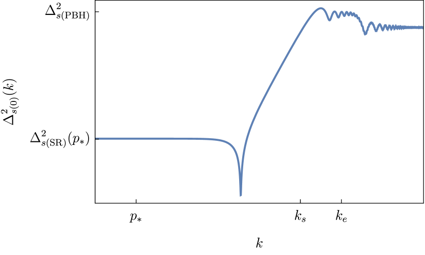
Figure 2: Power spectrum of the curvature perturbation. At CMB scale, $k\ll k_{s}$, the power spectrum is almost scale invariant. $p_{*}=0.05~{}\mathrm{Mpc}^{-1}$ is the pivot scale with amplitude $\Delta_{s(\mathrm{SR})}^{2}(p_{*})=2.1\times 10^{-9}$, based on observational result [31]. At small scale, between $k_{s}$ and $k_{e}$, the power spectrum is amplified to typically $\Delta_{s(\mathrm{PBH})}^{2}\sim\mathcal{O}(0.01)$ to form appreciable amount of PBHs.

So far, we have explained the tree-level contribution of the power spectrum. If we expand the action (1) until higher-order in curvature perturbation, we can calculate loop corrections to the power spectrum. Expanding (1) to third-order of $\zeta$ yields the interaction action [111]

$$S_{\mathrm{int}}=M_{\mathrm{pl}}^{2}\int\mathrm{d}t~{}\mathrm{d}^{3}x~{}a^{3}\left[\epsilon^{2}\dot{\zeta}^{2}\zeta+\frac{1}{a^{2}}\epsilon^{2}(\partial_{i}\zeta)^{2}\zeta\right.$$

$$\left.-2\epsilon\dot{\zeta}\partial_{i}\zeta\partial_{i}\chi-\frac{1}{2}\epsilon^{3}\dot{\zeta}^{2}\zeta+\frac{1}{2}\epsilon\zeta(\partial_{i}\partial_{j}\chi)^{2}+\frac{1}{2}\epsilon\dot{\eta}\dot{\zeta}\zeta^{2}\right],$$ (25)

where $\partial^{2}\chi=\epsilon\dot{\zeta}$. In standard SR inflation, the first three terms and the last three terms in (25) have coupling $\mathcal{O}(\epsilon^{2})$ and $\mathcal{O}(\epsilon^{3})$, respectively. The same situation happens in the context of inflation with PBH formation scenario, except the last term in (25), which has a coupling $\mathcal{O}(\epsilon)$ because $\eta$ can have $\mathcal{O}(1)$ transition [138, 139, 140, 141, 142], approximately from $0$ to $-6$.

We now calculate one-loop correction generated by cubic self-interaction (25) in the context of PBH formation using the standard in-in perturbation theory

$$\langle\mathcal{O(\tau)}\rangle=\left\langle\left[\bar{\mathrm{T}}\exp\left(i\int_{-\infty}^{\tau}\mathrm{d}\tau^{\prime}H_{\mathrm{int}}(\tau^{\prime})\right)\right]\mathcal{\hat{O}}(\tau)\right.$$

$$\left.\left[\mathrm{T}\exp\left(-i\int_{-\infty}^{\tau}\mathrm{d\tau^{\prime}}H_{\mathrm{int}}(\tau^{\prime})\right)\right]\right\rangle,$$ (26)

where $\mathcal{\hat{O}}(\tau)$ is an operator at a fixed time $\tau$, and $\mathrm{T}$ and $\bar{\mathrm{T}}$ denote time and antitime ordering. Also, $H_{\mathrm{int}}=-\int\mathrm{d}^{3}x~{}\mathcal{L}_{\mathrm{int}}$ is Hamiltonian corresponding to the Lagrangian $\mathcal{L}_{\mathrm{int}}$, defined by the integrand of (25). In our case, the operator is $\zeta(\mathbf{p})\zeta(-\mathbf{p})$, where $\mathbf{p}$ is CMB scale wavevector, evaluated at $\tau=\tau_{0}~{}(\rightarrow 0)$.

First-order expansion vanishes, yielding an odd-point correlation function. Second-order expansion of the perturbation theory is

$$\langle\mathcal{O(\tau)}\rangle=\langle\mathcal{O(\tau)}\rangle_{(0,2)}^{\dagger}+\langle\mathcal{O(\tau)}\rangle_{(1,1)}+\langle\mathcal{O(\tau)}\rangle_{(0,2)},$$ (27)

$$\langle\mathcal{O(\tau)}\rangle_{(1,1)}=\int_{-\infty}^{\tau}\mathrm{d}\tau_{1}\int_{-\infty}^{\tau}\mathrm{d}\tau_{2}\langle H_{\mathrm{int}}(\tau_{1})\mathcal{\hat{O}}(\tau)H_{\mathrm{int}}(\tau_{2})\rangle,$$

$$\langle\mathcal{O(\tau)}\rangle_{(0,2)}=-\int_{-\infty}^{\tau}\mathrm{d}\tau_{1}\int_{-\infty}^{\tau_{1}}\mathrm{d}\tau_{2}\langle\mathcal{\hat{O}}(\tau)H_{\mathrm{int}}(\tau_{1})H_{\mathrm{int}}(\tau_{2})\rangle.$$

The leading cubic self-interaction is the last term in (25) with interaction Hamiltonian

$$H_{\mathrm{int}}(\tau)=-\frac{1}{2}M_{\mathrm{pl}}^{2}\int\mathrm{d}^{3}x~{}\epsilon\eta^{\prime}a^{2}\zeta^{\prime}\zeta^{2}.$$ (28)

After substituting the interaction Hamiltonian to the perturbation theory, we find

$$\langle\zeta(\mathbf{p})\zeta(-\mathbf{p})\rangle_{(1,1)}= ~{}\frac{1}{4}M_{\mathrm{pl}}^{4}\int_{-\infty}^{0}\mathrm{d}\tau_{1}~{}a^{2}(\tau_{1})\epsilon(\tau_{1})\eta^{\prime}(\tau_{1})\int_{-\infty}^{0}\mathrm{d}\tau_{2}~{}a^{2}(\tau_{2})\epsilon(\tau_{2})\eta^{\prime}(\tau_{2})\int\prod_{a=1}^{6}\left[\frac{\mathrm{d}^{3}k_{a}}{(2\pi)^{3}}\right]\delta^{3}(\mathbf{k}_{1}+\mathbf{k}_{2}+\mathbf{k}_{3})~{}$$

$$\times\delta^{3}(\mathbf{k}_{4}+\mathbf{k}_{5}+\mathbf{k}_{6})\left\langle\zeta^{\prime}(\mathbf{k}_{1},\tau_{1})\zeta(\mathbf{k}_{2},\tau_{1})\zeta(\mathbf{k}_{3},\tau_{1})\zeta(\mathbf{p})\zeta(-\mathbf{p})\zeta^{\prime}(\mathbf{k}_{4},\tau_{2})\zeta(\mathbf{k}_{5},\tau_{2})\zeta(\mathbf{k}_{6},\tau_{2})\right\rangle,$$ (29)

$$\langle\zeta(\mathbf{p})\zeta(-\mathbf{p})\rangle_{(0,2)}= ~{}-\frac{1}{4}M_{\mathrm{pl}}^{4}\int_{-\infty}^{0}\mathrm{d}\tau_{1}~{}a^{2}(\tau_{1})\epsilon(\tau_{1})\eta^{\prime}(\tau_{1})\int_{-\infty}^{\tau_{1}}\mathrm{d}\tau_{2}~{}a^{2}(\tau_{2})\epsilon(\tau_{2})\eta^{\prime}(\tau_{2})\int\prod_{a=1}^{6}\left[\frac{\mathrm{d}^{3}k_{a}}{(2\pi)^{3}}\right]\delta^{3}(\mathbf{k}_{1}+\mathbf{k}_{2}+\mathbf{k}_{3})~{}$$

$$\times\delta^{3}(\mathbf{k}_{4}+\mathbf{k}_{5}+\mathbf{k}_{6})\left\langle\zeta(\mathbf{p})\zeta(-\mathbf{p})\zeta^{\prime}(\mathbf{k}_{1},\tau_{1})\zeta(\mathbf{k}_{2},\tau_{1})\zeta(\mathbf{k}_{3},\tau_{1})\zeta^{\prime}(\mathbf{k}_{4},\tau_{2})\zeta(\mathbf{k}_{5},\tau_{2})\zeta(\mathbf{k}_{6},\tau_{2})\right\rangle.$$ (30)

To evaluate the time integral, we note that $\eta$ is almost constant in both SR and USR periods, so $\eta^{\prime}(\tau)\approx 0$ except for sharp transitions around $\tau=\tau_{s}$ and $\tau=\tau_{e}$. Therefore, the time integral can be evaluated as

$$\int_{-\infty}^{0}\mathrm{d}\tau~{}\eta^{\prime}(\tau)f(\tau)=\Delta\eta~{}f(\tau_{e}),$$ (31)

where $f(\tau)$ is a general continuous function. We neglect contribution from $\tau=\tau_{s}$ because it is much smaller than that from $\tau=\tau_{e}$. Nevertheless, contribution from $\tau=\tau_{s}$ is essential to recover Maldacena’s theorem for the bispectrum, as we show in our companion paper [144]. Performing operator expansion and Wick contraction, we obtain total one-loop correction

$$\left\langle\!\left\langle\zeta(\mathbf{p})\zeta(-\mathbf{p})\right\rangle\!\right\rangle_{(1)}=\left\langle\!\left\langle\zeta(\mathbf{p})\zeta(-\mathbf{p})\right\rangle\!\right\rangle_{(1,1)}+2\mathrm{Re}\left\langle\!\left\langle\zeta(\mathbf{p})\zeta(-\mathbf{p})\right\rangle\!\right\rangle_{(0,2)}=\frac{1}{4}M_{\mathrm{pl}}^{4}\epsilon^{2}(\tau_{e})a^{4}(\tau_{e})(\Delta\eta)^{2}$$ (32)

$$\times\int\frac{\mathrm{d}^{3}k}{(2\pi)^{3}}\left\{\zeta_{p}(\tau_{0})\zeta_{p}^{*}(\tau_{0})\left(4\zeta_{p}^{\prime}\zeta_{p}^{\prime*}\zeta_{q}\zeta_{q}^{*}\zeta_{k}\zeta_{k}^{*}+8\zeta_{p}^{\prime*}\zeta_{p}\zeta_{q}^{\prime}\zeta_{q}^{*}\zeta_{k}\zeta_{k}^{*}+8\zeta_{p}^{\prime}\zeta_{p}^{*}\zeta_{q}^{\prime*}\zeta_{q}\zeta_{k}\zeta_{k}^{*}+16\zeta_{p}\zeta_{p}^{*}\zeta_{q}^{\prime}\zeta_{q}^{\prime*}\zeta_{k}\zeta_{k}^{*}\right)_{\tau=\tau_{e}}\right.$$

$$\left.-\mathrm{Re}\left[\zeta_{p}(\tau_{0})\zeta_{p}(\tau_{0})\left(4\zeta_{p}^{\prime*}\zeta_{p}^{\prime*}\zeta_{q}\zeta_{q}^{*}\zeta_{k}\zeta_{k}^{*}+8\zeta_{p}^{\prime*}\zeta_{p}^{*}\zeta_{q}^{\prime}\zeta_{q}^{*}\zeta_{k}\zeta_{k}^{*}+8\zeta_{p}^{\prime*}\zeta_{p}^{*}\zeta_{q}^{\prime*}\zeta_{q}\zeta_{k}\zeta_{k}^{*}+16\zeta_{p}^{*}\zeta_{p}^{*}\zeta_{q}^{\prime}\zeta_{q}^{\prime*}\zeta_{k}\zeta_{k}^{*}\right)_{\tau=\tau_{e}}\right]\right\},$$

where $\mathbf{q}=\mathbf{k}-\mathbf{p}$. After some algebra, for $p\ll k$, the leading term is simplified to

$$\left\langle\!\left\langle\zeta(\mathbf{p})\zeta(-\mathbf{p})\right\rangle\!\right\rangle_{(1)}=\frac{1}{4}M_{\mathrm{pl}}^{4}\epsilon^{2}(\tau_{e})a^{4}(\tau_{e})(\Delta\eta)^{2}\absolutevalue{\zeta_{p}(\tau_{0})}^{2}$$

$$\times 16\int\frac{\mathrm{d}^{3}k}{(2\pi)^{3}}\left[\absolutevalue{\zeta_{k}}^{2}~{}\mathrm{Im}(\zeta_{p}\zeta_{p}^{\prime*})~{}\mathrm{Im}(\zeta_{q}\zeta_{q}^{\prime*})\right]_{\tau=\tau_{e}}.$$ (33)

Expressing (14) in terms of curvature perturbation during USR period, we obtain

$$[\mathrm{Im}(\zeta_{q}\zeta_{q}^{\prime*})]_{\tau=\tau_{e}}=\frac{1}{4M_{\mathrm{pl}}^{2}\epsilon(\tau_{e})a^{2}(\tau_{e})},$$ (34)

which is independent of wavenumber $q$. It leads to commutation relation $[\zeta,\dot{\zeta}]\propto a^{3}$, which is in line with large quantum loop correction that we will find shortly. Then, substituting it to (33) yields one-loop correction to the power spectrum

$$\Delta_{s(1)}^{2}(p)=\frac{1}{4}(\Delta\eta)^{2}\Delta_{s(0)}^{2}(p)\int_{k_{\mathrm{IR}}}^{k_{\mathrm{UV}}}\frac{\mathrm{d}k}{k}\Delta^{2}_{s(0)}(k).$$ (35)

In principle, the wavenumber integral should be extended from well below CMB pivot scale $k_{\mathrm{IR}}\ll p_{*}=0.05~{}\mathrm{Mpc}^{-1}$ to ultraviolet (UV) cutoff scale $k_{\mathrm{UV}}\rightarrow\infty$. Contributions from large length scale including the CMB scale can be neglected because they are much smaller than those from amplified perturbation on small scale. On the other hand, contribution from UV scale diverges. Because we are interested in the finite effect of the amplified perturbation on specific small scale due to the USR period to one-loop correction, we conservatively restrict the wavenumber integration domain from $k_{\mathrm{IR}}=k_{s}$ to $k_{\mathrm{UV}}=k_{e}$. The UV cutoff issue will be discussed later. For $k_{\mathrm{UV}}/k_{\mathrm{IR}}=k_{e}/k_{s}\gg 1$, (35) reads

$$\Delta_{s(1)}^{2}(p)=\frac{1}{4}(\Delta\eta)^{2}\Delta_{s(0)}^{2}(p)\Delta_{s(\mathrm{PBH})}^{2}\left(1.1+\log\frac{k_{e}}{k_{s}}\right).$$ (36)

In order for the standard cosmological perturbation theory to be trustable, one-loop correction must be much smaller than the tree-level contribution, namely $\Delta_{s(1)}^{2}\ll\Delta_{s(0)}^{2}$. It leads to a strong inequality

$$\frac{1}{4}(\Delta\eta)^{2}\Delta_{s(\mathrm{PBH})}^{2}\left(1.1+\log\frac{k_{e}}{k_{s}}\right)\ll 1.$$ (37)

We can obtain a bound on $k_{e}/k_{s}$ by substituting numerical values $\Delta_{s(\mathrm{SR})}^{2}(p_{*})=2.1\times 10^{-9}$ and $n_{s}=0.9649\pm 0.0042$ at pivot scale based on observational result [31]. Also, $\Delta\eta=6$ as transition from USR to SR period. Solving inequality (37) numerically leads to an upper bound $k_{e}/k_{s}\ll 15$, which is equivalent to

$$\Delta_{s(\mathrm{PBH})}^{2}\ll\frac{1}{(\Delta\eta)^{2}}\simeq 0.03.$$ (38)

So far, we have considered finite contribution of superhorizon perturbation at $\tau=\tau_{e}$ to the one-loop correction. In addition, there is contribution from perturbations which are still inside the horizon at $\tau=\tau_{e}$. To identify such contributions, we introduce physical UV cutoff $\Lambda$ to the upper bound of wavenumber integral such as

$$\int_{k_{\mathrm{IR}}}^{k_{\mathrm{UV}}}\frac{\mathrm{d}k}{k}\Delta^{2}_{s(0)}(k)=\left(\int_{k_{s}}^{k_{e}}+\int_{k_{e}}^{\Lambda a(\tau_{e})}\right)\frac{\mathrm{d}k}{k}\Delta^{2}_{s(0)}(k).$$ (39)

Including the divergence, the one-loop correction is

$$\Delta_{s(1)}^{2}(p)=\frac{1}{4}(\Delta\eta)^{2}\Delta_{s(0)}^{2}(p)\Delta_{s(\mathrm{PBH})}^{2}$$

$$\times\left(1.1+\log\frac{k_{e}}{k_{s}}+\log\frac{\Lambda}{H}+\frac{\Lambda^{2}-H^{2}}{2H^{2}}\right).$$ (40)

The bare power spectrum at one-loop order is given by

$$\Delta_{s}^{2}(p)=\Delta_{s(0)}^{2}(p_{*})\left(\frac{p}{p_{*}}\right)^{n_{s}-1}\left\{1+\frac{1}{4}(\Delta\eta)^{2}\Delta_{s(\mathrm{PBH})}^{2}\right.$$

$$\left.\times\left(1.1+\log\frac{k_{e}}{k_{s}}+\log\tilde{\Lambda}+\frac{\tilde{\Lambda}^{2}-1}{2}\right)\right.$$

$$\left.+\mathcal{O}\left[\left((\Delta\eta)^{2}\Delta_{s(\mathrm{PBH})}^{2}\right)^{2}\right]\right\},$$ (41)

where $\tilde{\Lambda}=\Lambda/H$ is defined. Such power spectrum diverges as we take $\Lambda\rightarrow\infty$ limit . To make it finite, we need to renormalize order by order the coefficient $\Delta_{s(0)}^{2}(p_{*})$ so it depends on $\tilde{\Lambda}$. This procedure is equivalent to introducing a counterterm $\delta Z$, defined in $\Delta_{s(0)}^{2}(p_{*})\equiv(1+\delta Z)\Delta_{s(0)}^{2}(p_{*},\tilde{\mu})$. At one-loop order, after substituting (24), $\delta Z$ can be read off from the renormalized coefficient

$$\Delta_{s(0)}^{2}(p_{*})\equiv\Delta_{s(0)}^{2}(p_{*},\tilde{\mu})\left\{1+\frac{1}{4}(\Delta\eta)^{2}\Delta_{s(0)}^{2}(p_{*},\tilde{\mu})\right.$$

$$\left.\times\left(\frac{k_{e}}{k_{s}}\right)^{6}\left(-1.1-\log\frac{k_{e}}{k_{s}}+\log\frac{\tilde{\mu}}{\tilde{\Lambda}}+\frac{\tilde{\mu}^{2}-\tilde{\Lambda}^{2}}{2}\right)\right.$$

$$\left.+\mathcal{O}\left[\left((\Delta\eta)^{2}\Delta_{s(\mathrm{PBH})}^{2}\right)^{2}\right]\right\},$$ (42)

where $\tilde{\mu}=\mu/H$ with $\mu$ being a renormalization scale. Therefore, we obtained the renormalized power spectrum

$$\Delta_{s}^{2}(p)=\Delta_{s(0)}^{2}(p_{*},\tilde{\mu})\left(\frac{p}{p_{*}}\right)^{n_{s}-1}$$

$$\times\left\{1+\frac{1}{4}(\Delta\eta)^{2}\Delta_{s(0)}^{2}(p_{*},\tilde{\mu})\left(\frac{k_{e}}{k_{s}}\right)^{6}\left(\log\tilde{\mu}+\frac{\tilde{\mu}^{2}-1}{2}\right)\right.$$

$$\left.+\mathcal{O}\left[\left((\Delta\eta)^{2}\Delta_{s(\mathrm{PBH})}^{2}\right)^{2}\right]\right\}.$$ (43)

Taking renormalization scale $\mu=H$, the renormalized power spectrum reads

$$\Delta_{s}^{2}(p)= ~{}\Delta_{s(0)}^{2}(p_{*},\mu=H)\left(\frac{p}{p_{*}}\right)^{n_{s}-1}$$

$$\times\left\{1+\mathcal{O}\left[\left((\Delta\eta)^{2}\Delta_{s(\mathrm{PBH})}^{2}\right)^{2}\right]\right\},$$ (44)

where $\Delta_{s(0)}^{2}(p_{*},\mu=H)$ is fixed to the observed power spectrum $2.1\times 10^{-9}$.

Such order by order renormalization is justified if higher-order loop correction is suppressed compared to the lower-order one. In this context, this is possible only if $(\Delta\eta)^{2}\Delta_{s(\mathrm{PBH})}^{2}\ll 1$, which is the same condition as (38). Therefore, condition (38) is a necessary condition for the theory to be perturbative, or requirement to avoid strong coupling. Indeed, this perturbative coupling requirement is needed to justify the use of in-in perturbation theory (27). Although we focus on loop correction to large-scale power spectrum, such coupling also affects small-scale power spectrum and the same constraint is needed to avoid strong coupling.

In single-field inflation, PBH formation models can be classified into two categories [131]. The first category is models with features in the inflationary potential or non-minimally coupled inflaton with potential defined in the Einstein frame. Models with an extremely flat feature fall in this category including those with an inflection point in the potential [7, 42, 43, 44, 45, 46, 47, 48, 49, 50, 51, 55, 56, 57, 58, 59, 60, 61, 62, 52, 53, 54, 63, 64]. Other examples of feature are a tiny bump or dip [65, 66, 67, 68, 69, 70], an upward or downward step [71, 72, 74, 75, 73, 76], polynomial shape [77, 78, 79, 80] and Coleman-Weinberg potential [41, 81, 82]. In these examples, modification of potential makes a sharp $\eta$ transition on the inflaton dynamics.

The second category is models with modified gravity or beyond non-minimally coupled inflaton. For example, models based on $k$ [147] or $G$ [148] inflation [83, 84, 85], the effective field theory of inflation [86, 87, 88], $f(R)$ gravity [89], a non-minimal derivative coupling [90, 91], Gauss-Bonnet inflation [92], and bumpy axion inflation [93]. In these examples, amplification of small-scale perturbation can be realized by a sharp transition of $\eta$ and/or other parameters. In [86, 87], amplification of small-scale perturbation is caused by a sharp transition of the sound speed, $c_{s}$, a quantity that parametrizes deviation from canonical kinetic term. In this case, coupling $\eta^{\prime}$ in cubic self-interaction (28) is modified to $(\eta/c_{s}^{2})^{\prime}$ [112, 113], so such theory might also have large one-loop correction. Therefore, constraint $\Delta_{s(\mathrm{PBH})}^{2}\ll\mathcal{O}(0.01)$ can be imposed to almost every PBH formation model in single-field inflation that has been studied, although for a few number of models we have to examine it more carefully.

In conclusion, we have calculated the one-loop correction of the inflationary power spectrum in single-field inflation realizing PBH formation. We have shown that models realizing appreciable amount of PBH formation with the enhanced small-scale spectrum by USR inflaton dynamics inevitably induces nonperturbative coupling to the power spectrum on CMB scale. We therefore conclude that PBH formation from cosmological perturbation theory single-field inflation with an USR dynamics is ruled out.

J. K. thanks Hayato Motohashi for a fruitful discussion. J. K. acknowledges the support from JSPS KAKENHI Grant No. 22J20289 and Global Science Graduate Course (GSGC) program of The University of Tokyo. J. Y. is supported by JSPS KAKENHI Grant No. 20H05639 and Grant-in-Aid for Scientific Research on Innovative Areas 20H05248.

References

- Zel’dovich and Novikov [1967] Y. B. Zel’dovich and I. D. Novikov, Sov. Astron. 10, 602 (1967).
- Hawking [1971] S. Hawking, Mon. Not. Roy. Astron. Soc. 152, 75 (1971).
- Carr and Hawking [1974] B. J. Carr and S. W. Hawking, Mon. Not. Roy. Astron. Soc. 168, 399 (1974).
- Hawking [1974] S. W. Hawking, Nature 248, 30 (1974).
- Chapline [1975] G. F. Chapline, Nature 253, 251 (1975).
- Garcia-Bellido et al. [1996] J. Garcia-Bellido, A. D. Linde, and D. Wands, Phys. Rev. D 54, 6040 (1996), arXiv:astro-ph/9605094 .
- Ivanov et al. [1994] P. Ivanov, P. Naselsky, and I. Novikov, Phys. Rev. D 50, 7173 (1994).
- Yokoyama [1997] J. Yokoyama, Astron. Astrophys. 318, 673 (1997), arXiv:astro-ph/9509027 .
- Afshordi et al. [2003] N. Afshordi, P. McDonald, and D. N. Spergel, Astrophys. J. Lett. 594, L71 (2003), arXiv:astro-ph/0302035 .
- Frampton et al. [2010] P. H. Frampton, M. Kawasaki, F. Takahashi, and T. T. Yanagida, JCAP 04, 023 (2010), arXiv:1001.2308 [hep-ph] .
- Belotsky et al. [2014] K. M. Belotsky, A. D. Dmitriev, E. A. Esipova, V. A. Gani, A. V. Grobov, M. Y. Khlopov, A. A. Kirillov, S. G. Rubin, and I. V. Svadkovsky, Mod. Phys. Lett. A 29, 1440005 (2014), arXiv:1410.0203 [astro-ph.CO] .
- Carr et al. [2016] B. Carr, F. Kuhnel, and M. Sandstad, Phys. Rev. D 94, 083504 (2016), arXiv:1607.06077 [astro-ph.CO] .
- Inomata et al. [2017] K. Inomata, M. Kawasaki, K. Mukaida, Y. Tada, and T. T. Yanagida, Phys. Rev. D 96, 043504 (2017), arXiv:1701.02544 [astro-ph.CO] .
- Espinosa et al. [2018] J. R. Espinosa, D. Racco, and A. Riotto, Phys. Rev. Lett. 120, 121301 (2018), arXiv:1710.11196 [hep-ph] .
- Green and Kavanagh [2021] A. M. Green and B. J. Kavanagh, J. Phys. G 48, 043001 (2021), arXiv:2007.10722 [astro-ph.CO] .
- Carr and Kuhnel [2020] B. Carr and F. Kuhnel, Ann. Rev. Nucl. Part. Sci. 70, 355 (2020), arXiv:2006.02838 [astro-ph.CO] .
- Sasaki et al. [2016] M. Sasaki, T. Suyama, T. Tanaka, and S. Yokoyama, Phys. Rev. Lett. 117, 061101 (2016), [Erratum: Phys.Rev.Lett. 121, 059901 (2018)], arXiv:1603.08338 [astro-ph.CO] .
- Raidal et al. [2017] M. Raidal, V. Vaskonen, and H. Veermäe, JCAP 09, 037 (2017), arXiv:1707.01480 [astro-ph.CO] .
- Ali-Haïmoud et al. [2017] Y. Ali-Haïmoud, E. D. Kovetz, and M. Kamionkowski, Phys. Rev. D 96, 123523 (2017), arXiv:1709.06576 [astro-ph.CO] .
- Raidal et al. [2019] M. Raidal, C. Spethmann, V. Vaskonen, and H. Veermäe, JCAP 02, 018 (2019), arXiv:1812.01930 [astro-ph.CO] .
- Vaskonen and Veermäe [2020] V. Vaskonen and H. Veermäe, Phys. Rev. D 101, 043015 (2020), arXiv:1908.09752 [astro-ph.CO] .
- Hall et al. [2020] A. Hall, A. D. Gow, and C. T. Byrnes, Phys. Rev. D 102, 123524 (2020), arXiv:2008.13704 [astro-ph.CO] .
- Mukhanov and Chibisov [1981] V. F. Mukhanov and G. V. Chibisov, JETP Lett. 33, 532 (1981).
- Hawking [1982] S. W. Hawking, Phys. Lett. B 115, 295 (1982).
- Guth and Pi [1982] A. H. Guth and S. Y. Pi, Phys. Rev. Lett. 49, 1110 (1982).
- Starobinsky [1982] A. A. Starobinsky, Phys. Lett. B 117, 175 (1982).
- Starobinsky [1980] A. A. Starobinsky, Phys. Lett. B 91, 99 (1980).
- Sato [1981] K. Sato, Mon. Not. Roy. Astron. Soc. 195, 467 (1981).
- Guth [1981] A. H. Guth, Phys. Rev. D 23, 347 (1981).
- Aghanim et al. [2020] N. Aghanim et al. (Planck), Astron. Astrophys. 641, A1 (2020), arXiv:1807.06205 [astro-ph.CO] .
- Akrami et al. [2020a] Y. Akrami et al. (Planck), Astron. Astrophys. 641, A10 (2020a), arXiv:1807.06211 [astro-ph.CO] .
- Akrami et al. [2020b] Y. Akrami et al. (Planck), Astron. Astrophys. 641, A9 (2020b), arXiv:1905.05697 [astro-ph.CO] .
- Nakama et al. [2014] T. Nakama, T. Suyama, and J. Yokoyama, Phys. Rev. Lett. 113, 061302 (2014), arXiv:1403.5407 [astro-ph.CO] .
- Jeong et al. [2014] D. Jeong, J. Pradler, J. Chluba, and M. Kamionkowski, Phys. Rev. Lett. 113, 061301 (2014), arXiv:1403.3697 [astro-ph.CO] .
- Inomata et al. [2016] K. Inomata, M. Kawasaki, and Y. Tada, Phys. Rev. D 94, 043527 (2016), arXiv:1605.04646 [astro-ph.CO] .
- Nakama et al. [2018] T. Nakama, T. Suyama, K. Kohri, and N. Hiroshima, Phys. Rev. D 97, 023539 (2018), arXiv:1712.08820 [astro-ph.CO] .
- Kawasaki et al. [2022] M. Kawasaki, H. Nakatsuka, and K. Nakayama, JCAP 03, 061 (2022), arXiv:2110.12620 [astro-ph.CO] .
- Kimura et al. [2021] R. Kimura, T. Suyama, M. Yamaguchi, and Y.-L. Zhang, JCAP 04, 031 (2021), arXiv:2102.05280 [astro-ph.CO] .
- Wang et al. [2023] X. Wang, Y.-l. Zhang, R. Kimura, and M. Yamaguchi, Sci. China Phys. Mech. Astron. 66, 260462 (2023), arXiv:2209.12911 [astro-ph.CO] .
- Carr and Lidsey [1993] B. J. Carr and J. E. Lidsey, Phys. Rev. D 48, 543 (1993).
- Yokoyama [1998] J. Yokoyama, Phys. Rev. D 58, 083510 (1998), arXiv:astro-ph/9802357 .
- Kawasaki et al. [1998] M. Kawasaki, N. Sugiyama, and T. Yanagida, Phys. Rev. D 57, 6050 (1998), arXiv:hep-ph/9710259 .
- Kawasaki and Yanagida [1999] M. Kawasaki and T. Yanagida, Phys. Rev. D 59, 043512 (1999), arXiv:hep-ph/9807544 .
- Kawasaki et al. [2016] M. Kawasaki, A. Kusenko, Y. Tada, and T. T. Yanagida, Phys. Rev. D 94, 083523 (2016), arXiv:1606.07631 [astro-ph.CO] .
- Gao and Guo [2018] T.-J. Gao and Z.-K. Guo, Phys. Rev. D 98, 063526 (2018), arXiv:1806.09320 [hep-ph] .
- Nanopoulos et al. [2020] D. V. Nanopoulos, V. C. Spanos, and I. D. Stamou, Phys. Rev. D 102, 083536 (2020), arXiv:2008.01457 [astro-ph.CO] .
- Wu et al. [2021] L. Wu, Y. Gong, and T. Li, Phys. Rev. D 104, 123544 (2021), arXiv:2105.07694 [gr-qc] .
- Stamou [2021] I. D. Stamou, Phys. Rev. D 103, 083512 (2021), arXiv:2104.08654 [hep-ph] .
- Cheng et al. [2018] S.-L. Cheng, W. Lee, and K.-W. Ng, JCAP 07, 001 (2018), arXiv:1801.09050 [astro-ph.CO] .
- Ballesteros et al. [2020a] G. Ballesteros, J. Rey, and F. Rompineve, JCAP 06, 014 (2020a), arXiv:1912.01638 [astro-ph.CO] .
- Pi et al. [2018] S. Pi, Y.-l. Zhang, Q.-G. Huang, and M. Sasaki, JCAP 05, 042 (2018), arXiv:1712.09896 [astro-ph.CO] .
- Dalianis and Tringas [2019] I. Dalianis and G. Tringas, Phys. Rev. D 100, 083512 (2019), arXiv:1905.01741 [astro-ph.CO] .
- Dalianis et al. [2019] I. Dalianis, A. Kehagias, and G. Tringas, JCAP 01, 037 (2019), arXiv:1805.09483 [astro-ph.CO] .
- Mahbub [2020] R. Mahbub, Phys. Rev. D 101, 023533 (2020), arXiv:1910.10602 [astro-ph.CO] .
- Cicoli et al. [2018] M. Cicoli, V. A. Diaz, and F. G. Pedro, JCAP 06, 034 (2018), arXiv:1803.02837 [hep-th] .
- Özsoy et al. [2018] O. Özsoy, S. Parameswaran, G. Tasinato, and I. Zavala, JCAP 07, 005 (2018), arXiv:1803.07626 [hep-th] .
- Cicoli et al. [2022] M. Cicoli, F. G. Pedro, and N. Pedron, JCAP 08, 030 (2022), arXiv:2203.00021 [hep-th] .
- Ezquiaga et al. [2018] J. M. Ezquiaga, J. Garcia-Bellido, and E. Ruiz Morales, Phys. Lett. B 776, 345 (2018), arXiv:1705.04861 [astro-ph.CO] .
- Ballesteros and Taoso [2018] G. Ballesteros and M. Taoso, Phys. Rev. D 97, 023501 (2018), arXiv:1709.05565 [hep-ph] .
- Drees and Xu [2021] M. Drees and Y. Xu, Eur. Phys. J. C 81, 182 (2021), arXiv:1905.13581 [hep-ph] .
- Cheong et al. [2021] D. Y. Cheong, S. M. Lee, and S. C. Park, JCAP 01, 032 (2021), arXiv:1912.12032 [hep-ph] .
- Rasanen and Tomberg [2019] S. Rasanen and E. Tomberg, JCAP 01, 038 (2019), arXiv:1810.12608 [astro-ph.CO] .
- Garcia-Bellido and Ruiz Morales [2017] J. Garcia-Bellido and E. Ruiz Morales, Phys. Dark Univ. 18, 47 (2017), arXiv:1702.03901 [astro-ph.CO] .
- Ragavendra et al. [2021] H. V. Ragavendra, P. Saha, L. Sriramkumar, and J. Silk, Phys. Rev. D 103, 083510 (2021), arXiv:2008.12202 [astro-ph.CO] .
- Mishra and Sahni [2020] S. S. Mishra and V. Sahni, JCAP 04, 007 (2020), arXiv:1911.00057 [gr-qc] .
- Atal et al. [2019] V. Atal, J. Garriga, and A. Marcos-Caballero, JCAP 09, 073 (2019), arXiv:1905.13202 [astro-ph.CO] .
- Zheng et al. [2022] R. Zheng, J. Shi, and T. Qiu, Chin. Phys. C 46, 045103 (2022), arXiv:2106.04303 [astro-ph.CO] .
- Wang et al. [2021] Q. Wang, Y.-C. Liu, B.-Y. Su, and N. Li, Phys. Rev. D 104, 083546 (2021), arXiv:2111.10028 [astro-ph.CO] .
- Rezazadeh et al. [2022] K. Rezazadeh, Z. Teimoori, S. Karimi, and K. Karami, Eur. Phys. J. C 82, 758 (2022), arXiv:2110.01482 [gr-qc] .
- Iacconi et al. [2022] L. Iacconi, H. Assadullahi, M. Fasiello, and D. Wands, JCAP 06, 007 (2022), arXiv:2112.05092 [astro-ph.CO] .
- Cai et al. [2022] Y.-F. Cai, X.-H. Ma, M. Sasaki, D.-G. Wang, and Z. Zhou, Phys. Lett. B 834, 137461 (2022), arXiv:2112.13836 [astro-ph.CO] .
- Kefala et al. [2021] K. Kefala, G. P. Kodaxis, I. D. Stamou, and N. Tetradis, Phys. Rev. D 104, 023506 (2021), arXiv:2010.12483 [astro-ph.CO] .
- Inomata et al. [2021] K. Inomata, E. McDonough, and W. Hu, Phys. Rev. D 104, 123553 (2021), arXiv:2104.03972 [astro-ph.CO] .
- Ng and Wu [2021] K.-W. Ng and Y.-P. Wu, JHEP 11, 076 (2021), arXiv:2102.05620 [astro-ph.CO] .
- Motohashi et al. [2020] H. Motohashi, S. Mukohyama, and M. Oliosi, JCAP 03, 002 (2020), arXiv:1910.13235 [gr-qc] .
- Inomata et al. [2022] K. Inomata, E. McDonough, and W. Hu, JCAP 02, 031 (2022), arXiv:2110.14641 [astro-ph.CO] .
- Hertzberg and Yamada [2018] M. P. Hertzberg and M. Yamada, Phys. Rev. D 97, 083509 (2018), arXiv:1712.09750 [astro-ph.CO] .
- Ballesteros et al. [2020b] G. Ballesteros, J. Rey, M. Taoso, and A. Urbano, JCAP 07, 025 (2020b), arXiv:2001.08220 [astro-ph.CO] .
- Kannike et al. [2017] K. Kannike, L. Marzola, M. Raidal, and H. Veermäe, JCAP 09, 020 (2017), arXiv:1705.06225 [astro-ph.CO] .
- Di and Gong [2018] H. Di and Y. Gong, JCAP 07, 007 (2018), arXiv:1707.09578 [astro-ph.CO] .
- Saito et al. [2008] R. Saito, J. Yokoyama, and R. Nagata, JCAP 06, 024 (2008), arXiv:0804.3470 [astro-ph] .
- Bugaev and Klimai [2008] E. Bugaev and P. Klimai, Phys. Rev. D 78, 063515 (2008), arXiv:0806.4541 [astro-ph] .
- Solbi and Karami [2021a] M. Solbi and K. Karami, JCAP 08, 056 (2021a), arXiv:2102.05651 [astro-ph.CO] .
- Solbi and Karami [2021b] M. Solbi and K. Karami, Eur. Phys. J. C 81, 884 (2021b), arXiv:2106.02863 [astro-ph.CO] .
- Teimoori et al. [2021] Z. Teimoori, K. Rezazadeh, M. A. Rasheed, and K. Karami, JCAP 2021, 018 (2021), arXiv:2107.07620 [astro-ph.CO] .
- Ballesteros et al. [2019] G. Ballesteros, J. Beltran Jimenez, and M. Pieroni, JCAP 06, 016 (2019), arXiv:1811.03065 [astro-ph.CO] .
- Ballesteros et al. [2022] G. Ballesteros, S. Céspedes, and L. Santoni, JHEP 01, 074 (2022), arXiv:2109.00567 [hep-th] .
- Ashoorioon et al. [2021] A. Ashoorioon, A. Rostami, and J. T. Firouzjaee, JHEP 07, 087 (2021), arXiv:1912.13326 [astro-ph.CO] .
- Frolovsky et al. [2022] D. Frolovsky, S. V. Ketov, and S. Saburov, Mod. Phys. Lett. A 37, 2250135 (2022), arXiv:2205.00603 [astro-ph.CO] .
- Fu et al. [2019] C. Fu, P. Wu, and H. Yu, Phys. Rev. D 100, 063532 (2019), arXiv:1907.05042 [astro-ph.CO] .
- Heydari and Karami [2022] S. Heydari and K. Karami, Eur. Phys. J. C 82, 83 (2022), arXiv:2107.10550 [gr-qc] .
- Kawai and Kim [2021] S. Kawai and J. Kim, Phys. Rev. D 104, 083545 (2021), arXiv:2108.01340 [astro-ph.CO] .
- Özsoy and Lalak [2021] O. Özsoy and Z. Lalak, JCAP 01, 040 (2021), arXiv:2008.07549 [astro-ph.CO] .
- Carr et al. [2010] B. J. Carr, K. Kohri, Y. Sendouda, and J. Yokoyama, Phys. Rev. D 81, 104019 (2010), arXiv:0912.5297 [astro-ph.CO] .
- Carr et al. [2021] B. Carr, K. Kohri, Y. Sendouda, and J. Yokoyama, Rept. Prog. Phys. 84, 116902 (2021), arXiv:2002.12778 [astro-ph.CO] .
- Assadullahi and Wands [2010] H. Assadullahi and D. Wands, Phys. Rev. D 81, 023527 (2010), arXiv:0907.4073 [astro-ph.CO] .
- Baumann et al. [2007] D. Baumann, P. J. Steinhardt, K. Takahashi, and K. Ichiki, Phys. Rev. D 76, 084019 (2007), arXiv:hep-th/0703290 .
- Saito and Yokoyama [2009] R. Saito and J. Yokoyama, Phys. Rev. Lett. 102, 161101 (2009), [Erratum: Phys.Rev.Lett. 107, 069901 (2011)], arXiv:0812.4339 [astro-ph] .
- Saito and Yokoyama [2010] R. Saito and J. Yokoyama, Prog. Theor. Phys. 123, 867 (2010), [Erratum: Prog.Theor.Phys. 126, 351–352 (2011)], arXiv:0912.5317 [astro-ph.CO] .
- Cai et al. [2019] R.-g. Cai, S. Pi, and M. Sasaki, Phys. Rev. Lett. 122, 201101 (2019), arXiv:1810.11000 [astro-ph.CO] .
- Yokoyama [2021] J. Yokoyama, AAPPS Bull. 31, 17 (2021), arXiv:2105.07629 [gr-qc] .
- Sato and Yokoyama [2015] K. Sato and J. Yokoyama, Int. J. Mod. Phys. D 24, 1530025 (2015).
- Polarski and Starobinsky [1996] D. Polarski and A. A. Starobinsky, Class. Quant. Grav. 13, 377 (1996), arXiv:gr-qc/9504030 .
- Kinney [1997] W. H. Kinney, Phys. Rev. D 56, 2002 (1997), arXiv:hep-ph/9702427 .
- Yokoyama and Inoue [2002] J. Yokoyama and S. Inoue, Phys. Lett. B 524, 15 (2002), arXiv:hep-ph/0104083 .
- Kinney [2005] W. H. Kinney, Phys. Rev. D 72, 023515 (2005), arXiv:gr-qc/0503017 .
- Martin et al. [2013] J. Martin, H. Motohashi, and T. Suyama, Phys. Rev. D 87, 023514 (2013), arXiv:1211.0083 [astro-ph.CO] .
- Motohashi and Hu [2017] H. Motohashi and W. Hu, Phys. Rev. D 96, 063503 (2017), arXiv:1706.06784 [astro-ph.CO] .
- Yokoyama [1999] J. Yokoyama, Phys. Rev. D 59, 107303 (1999).
- Motohashi et al. [2015] H. Motohashi, A. A. Starobinsky, and J. Yokoyama, JCAP 09, 018 (2015), arXiv:1411.5021 [astro-ph.CO] .
- Maldacena [2003] J. M. Maldacena, JHEP 05, 013 (2003), arXiv:astro-ph/0210603 .
- Chen et al. [2007] X. Chen, M.-x. Huang, S. Kachru, and G. Shiu, JCAP 01, 002 (2007), arXiv:hep-th/0605045 .
- Seery and Lidsey [2005] D. Seery and J. E. Lidsey, JCAP 06, 003 (2005), arXiv:astro-ph/0503692 .
- Weinberg [2005] S. Weinberg, Phys. Rev. D 72, 043514 (2005), arXiv:hep-th/0506236 .
- Sloth [2006] M. S. Sloth, Nucl. Phys. B 748, 149 (2006), arXiv:astro-ph/0604488 .
- Seery [2008] D. Seery, JCAP 02, 006 (2008), arXiv:0707.3378 [astro-ph] .
- Bartolo et al. [2010] N. Bartolo, E. Dimastrogiovanni, and A. Vallinotto, JCAP 11, 003 (2010), arXiv:1006.0196 [astro-ph.CO] .
- Senatore and Zaldarriaga [2010] L. Senatore and M. Zaldarriaga, JHEP 12, 008 (2010), arXiv:0912.2734 [hep-th] .
- del Rio et al. [2018] A. del Rio, R. Durrer, and S. P. Patil, JHEP 12, 094 (2018), arXiv:1808.09282 [gr-qc] .
- Melville and Pajer [2021] S. Melville and E. Pajer, JHEP 05, 249 (2021), arXiv:2103.09832 [hep-th] .
- Kristiano and Yokoyama [2022a] J. Kristiano and J. Yokoyama, Phys. Rev. Lett. 128, 061301 (2022a), arXiv:2104.01953 [hep-th] .
- Kristiano and Yokoyama [2022b] J. Kristiano and J. Yokoyama, JCAP 07, 007 (2022b), arXiv:2204.05202 [hep-th] .
- Firouzjahi et al. [2019] H. Firouzjahi, A. Nassiri-Rad, and M. Noorbala, JCAP 01, 040 (2019), arXiv:1811.02175 [hep-th] .
- Cheng et al. [2022] S.-L. Cheng, D.-S. Lee, and K.-W. Ng, Phys. Lett. B 827, 136956 (2022), arXiv:2106.09275 [astro-ph.CO] .
- Syu et al. [2020] W.-C. Syu, D.-S. Lee, and K.-W. Ng, Phys. Rev. D 101, 025013 (2020), arXiv:1907.13089 [gr-qc] .
- Ando and Vennin [2021] K. Ando and V. Vennin, JCAP 04, 057 (2021), arXiv:2012.02031 [astro-ph.CO] .
- Meng et al. [2022] D.-S. Meng, C. Yuan, and Q.-g. Huang, Phys. Rev. D 106, 063508 (2022), arXiv:2207.07668 [astro-ph.CO] .
- Chen et al. [2023] C. Chen, A. Ota, H.-Y. Zhu, and Y. Zhu, Phys. Rev. D 107, 083518 (2023), arXiv:2210.17176 [astro-ph.CO] .
- Inomata et al. [2023] K. Inomata, M. Braglia, X. Chen, and S. Renaux-Petel, JCAP 04, 011 (2023), arXiv:2211.02586 [astro-ph.CO] .
- Sasaki [1986] M. Sasaki, Prog. Theor. Phys. 76, 1036 (1986).
- Karam et al. [2023] A. Karam, N. Koivunen, E. Tomberg, V. Vaskonen, and H. Veermäe, JCAP 03, 013 (2023), arXiv:2205.13540 [astro-ph.CO] .
- Starobinsky [1992] A. A. Starobinsky, JETP Lett. 55, 489 (1992).
- Leach et al. [2001] S. M. Leach, M. Sasaki, D. Wands, and A. R. Liddle, Phys. Rev. D 64, 023512 (2001), arXiv:astro-ph/0101406 .
- Byrnes et al. [2019] C. T. Byrnes, P. S. Cole, and S. P. Patil, JCAP 06, 028 (2019), arXiv:1811.11158 [astro-ph.CO] .
- Liu et al. [2020] J. Liu, Z.-K. Guo, and R.-G. Cai, Phys. Rev. D 101, 083535 (2020), arXiv:2003.02075 [astro-ph.CO] .
- Tasinato [2021] G. Tasinato, Phys. Rev. D 103, 023535 (2021), arXiv:2012.02518 [hep-th] .
- Pi and Wang [2023] S. Pi and J. Wang, JCAP 06, 018 (2023), arXiv:2209.14183 [astro-ph.CO] .
- Namjoo et al. [2013] M. H. Namjoo, H. Firouzjahi, and M. Sasaki, EPL 101, 39001 (2013), arXiv:1210.3692 [astro-ph.CO] .
- Cai et al. [2016] Y.-F. Cai, J.-O. Gong, D.-G. Wang, and Z. Wang, JCAP 10, 017 (2016), arXiv:1607.07872 [astro-ph.CO] .
- Chen et al. [2013] X. Chen, H. Firouzjahi, E. Komatsu, M. H. Namjoo, and M. Sasaki, JCAP 12, 039 (2013), arXiv:1308.5341 [astro-ph.CO] .
- Cai et al. [2018] Y.-F. Cai, X. Chen, M. H. Namjoo, M. Sasaki, D.-G. Wang, and Z. Wang, JCAP 05, 012 (2018), arXiv:1712.09998 [astro-ph.CO] .
- Davies et al. [2022] M. W. Davies, P. Carrilho, and D. J. Mulryne, JCAP 06, 019 (2022), arXiv:2110.08189 [astro-ph.CO] .
- Note [1] Strictly speaking, this interaction Hamiltonian is a function of redefined field , which is first introduced by Maldacena [111]. The relation between and is , where dots represent SR or superhorizon suppressed term. It is shown that field redefinition method is equivalent to considering boundary interaction [149]. Moreover, quartic self-interaction with first-order perturbation theory might generate the same order of one-loop correction to cubic self-interaction with second-order perturbation theory. Based on [150], such contribution from quartic self-interaction generates much smaller one-loop correction than those induced by the cubic self-interaction.
- [144] J. Kristiano and J. Yokoyama, arXiv:2303.00341 [hep-th] .
- Note [2] This can be derived by introducing physical wavenumber cutoff to the upper bound of wavenumber integral in (29) and (30). After performing time integral (31), the cutoff is evaluated at , which leads to (39).
- Note [3] Dimensional regularization leads to a similar expression, except is changed to , where is a small correction to the spatial dimension. Another difference is dimensional regularization cannot capture the quadratic divergence , as expected. Compared to one-loop computation for case considered in [118, 119], the time integral in our case is dominated by , not CMB horizon crossing time .
- Armendariz-Picon et al. [1999] C. Armendariz-Picon, T. Damour, and V. F. Mukhanov, Phys. Lett. B 458, 209 (1999), arXiv:hep-th/9904075 .
- Kobayashi et al. [2011] T. Kobayashi, M. Yamaguchi, and J. Yokoyama, Prog. Theor. Phys. 126, 511 (2011), arXiv:1105.5723 [hep-th] .
- Arroja and Tanaka [2011] F. Arroja and T. Tanaka, JCAP 05, 005 (2011), arXiv:1103.1102 [astro-ph.CO] .
- Jarnhus and Sloth [2008] P. R. Jarnhus and M. S. Sloth, JCAP 02, 013 (2008), arXiv:0709.2708 [hep-th] .