Topological phase transition between non-high symmetry critical phases and curvature function renormalization group

Abstract

The interplay between topology and criticality has been a recent interest of study in condensed matter physics. A unique topological transition between certain critical phases has been observed as a consequence of the edge modes living at criticalities. In this work, we generalize this phenomenon by investigating possible transitions between critical phases which are non-high symmetry in nature. We find the triviality and non-triviality of these critical phases in terms of the decay length of the edge modes and also characterize them using the winding numbers. The distinct non-high symmetry critical phases are separated by multicritical points with linear dispersion at which the winding number exhibits the quantized jump, indicating a change in the topology (number of edge modes) at the critical phases. Moreover, we reframe the scaling theory based on the curvature function, i.e. curvature function renormalization group method to efficiently address the non-high symmetry criticalities and multicriticalities. Using this we identify the conventional topological transition between gapped phases through non-high symmetry critical points, and also the unique topological transition between critical phases through multicritical points. The renormalization group flow, critical exponents and correlation function of Wannier states enable the characterization of non-high symmetry criticalities along with multicriticalities.

I Introduction

Topological states of matter have recieved a huge attention from both theoretical and experimental physicists in recent years haldane1988model ; hasan2010colloquium ; wang2017topological ; goldman2016topological ; narang2021topology . Non-trivial topology of the electronic band structure dictates the formation of localized stable edge modes which are protected by the bulk gap kitaev2001unpaired ; kane2005quantum . Number of edge modes are counted using topological invariant number, which is defined as the integral of the curvature function (Berry connection, Berry curvature, etc) over the Brillouin zone thouless1982quantized ; berry1984quantal ; zak1989berry . The topological invariant shows quantized jump associated with the bulk gap closing at a critical point. Therefore, a topological transition between distinct gapped phases is characterized by the bulk gap closing and opening along with the quantized jump in the values of invariant numbers altland1997symmetry ; sarkar2018quantization ; rahul2019interplay ; kartik2021topological .

Moreover, the quantization signifies the divergence in the curvature function at the critical point, which allows one to frame a scaling theory and correlation factors using the curvature function chen2016scaling ; chen2016scalinginvariant ; chen2017correlation ; chen2018weakly ; chen2019universality ; molignini2018universal ; panahiyan2020fidelity ; molignini2020generating ; abdulla2020curvature ; malard2020scaling ; molignini2020unifying ; kumar2021multi . A renormalization group (RG) method developed by iteratively finding a parameter space away from the critical point such as to reduce the divergence in the curvature function by driving it to its fixed point configuration. As this procedure does not change the topology of the band structure, eventually, the RG flow lines characterize the topological phase transition. The Lorentzian form of the curvature function near a critical point allows one to obtain the decay length of the edge modes at gapped topological phasesmolignini2018universal ; continentino2020finite . The decay length diverges on approaching a critical point, indicating the edge modes decays into the bulk. Therefore, the edge modes were believed to exist only with a finite bulk gap.

Recently, this conventional understanding has been re-investigated and the edge modes are observed to be localized and stable even at certain critical points verresen2018topology ; verresen2019gapless ; jones2019asymptotic ; verresen2020topology ; rahul2021majorana ; niu2021emergent ; PhysRevB.104.075132 ; PhysRevResearch.3.043048 ; fraxanet2021topological ; keselman2015gapless ; scaffidi2017gapless ; duque2021topological ; kumar2021topological . Therefore, similar to the gapped topological phases, certain critical phases also possess localized stable edge modes. The critical phases with topological and non-topological characters are identified as the high symmetry (HS) in nature since the gap closing occurs at the HS points in momentum space kumar2021topological . The distinct HS critical phases are separated by the multicritical points and favor an unusual topological transition between them. This transition occurs without gap closing and opening at HS points in contrast to the conventional topological transition kumar2021topological ; kumar2021multi ; rahul2021majorana ; verresen2020topology . The multicritical points which favor the transition are found to have quadratic dispersion. In general, they are the intersection points of the distinct criticalities and are studied in different contexts rufo2019multicritical ; malard2020multicriticality ; malard2020multicriticality ; sim2022quench . The scaling theory developed to identify the topological transition between gapped phases, are reframed to identify the topological transition between HS critical phases kumar2021topological ; kumar2021multi . The RG flow lines, correlation factors and decay length of edge modes at criticality, effectively characterized the topological transition kumar2021topological .

In the topological systems, increasing the nearest-neighbor couplings leads to prominent behavior of non-high symmetry (non-HS) critical points apart from the HS ones hsu2020topological ; niu2012majorana . The existence of stable localized edge modes at non-HS critical phases has not been explored previously. Furthermore, the possibility of unique topological transition between distinct non-HS critical phases is an interesting open question and require a detailed investigation. On the other hand, scaling theory based on the curvature function fails to capture the topological transition at a non-HS critical point between gapped phases abdulla2020curvature ; malard2020scaling . Therefore, the generalization of this method to identify the possible topological transition between non-HS critical phases is not straightforward.

Therefore, in the present work, our motivation is threefold. (i) We generalize the curvature function renormalization group (CRG) theory to characterize the non-HS quantum criticality. We develop and perform the CRG to identify the topological transition, at a non-HS critical point, between gapped phases. (ii) We identify the topological and trivial non-HS critical phases by investigating the existence of edge modes both analytically and numerically. (iii) We identify and explore the unique topological phase transition between non-HS critical phases via multicritical points. We reframe the CRG method to capture the topological transition, at a multicritical point, between non-HS critical phases.

The article is laid out as follows: In Section.II we introduce the model and the topological phase diagrams. Section.III describes the CRG method for topological transition at non-HS critical point between gapped phases. The diverging property, critical exponents and correlation factors using curvature functions are discussed. In Section.IV we demonstrate the existence of trivial and topological non-HS critical phases and the edge mode localizations. These results are supported by the winding number calculations and numerical analysis carried at non-HS criticality. In Section.V, the CRG method for topological transition at multicritical point between non-HS critical phases is discussed. We also discuss the behavior of curvature function, its exponents and the correlation factors at non-HS criticalities. We discuss the results and its experimental observabilities in Section.VI and finally conclude.

II Model and Topological Phase Diagram

We consider one dimensional lattice chain of spinless fermions in momentum space with onsite potential ($\Gamma_{0}$), nearest neighbor ($\Gamma_{1}$), next-nearest neighbor ($\Gamma_{2}$), and next-next-nearest neighbor ($\Gamma_{3}$) couplings. The two-band Bloch Hamiltonian can be written in the pseudospin basis as

$$\mathcal{H}(k,\boldsymbol{\Gamma})=\boldsymbol{\chi(k).\sigma}=\chi_{x}(k)\sigma_{x}+\chi_{y}(k)\sigma_{y}+\chi_{z}(k)\sigma_{z},$$ (1)

where $\boldsymbol{\Gamma}=\left\{\Gamma_{0},\Gamma_{1},\Gamma_{2},\Gamma_{3}\right\}$, $\chi_{x}(k)=\Gamma_{0}+\Gamma_{1}\cos k+\Gamma_{2}\cos 2k+\Gamma_{3}\cos 3k,$ $\chi_{y}(k)=\Gamma_{1}\sin k+\Gamma_{2}\sin 2k+\Gamma_{3}\sin 3k$, $\chi_{z}(k)=0$ and $\boldsymbol{\sigma}=(\sigma_{x},\sigma_{y},\sigma_{z})$ are the Pauli matrices. The model represents the 1D topological insulator and superconductor with extended nearest neighbor couplingsPhysRevLett.42.1698 ; kitaev2001unpaired ; hsu2020topological ; niu2012majorana ; kumar2021topological . Topological distinct gapped phases of the model can be identified with the winding number

$$w=\frac{1}{2\pi}\oint\limits_{BZ}\frac{\chi_{x}\partial_{k}\chi_{y}-\chi_{y}\partial_{k}\chi_{x}}{\chi_{x}^{2}+\chi_{y}^{2}}dk,$$ (2)

where $w\in\mathbb{Z}$ (integer), as shown in Fig.1. Topological phase transitions between distinct gapped phases are associated with the gap closing, $E_{k}=\pm\sqrt{\chi_{x}^{2}+\chi_{y}^{2}}=0$. This dictates the critical lines across which the winding number changes.

The gap closing momenta $k_{0}$ (critical momenta) in the Brillouin zone can be either HS or non-HS in nature. The momenta with $k_{0}=-k_{0}$, (up to a reciprocal lattice vector) are referred to as the HS points and are associated with space-group symmetries murakami2011gap ; kourtis2017weyl ; chen2019universality . In our model, there are two HS points at $k_{0}=0,\pm\pi$, as shown in Fig.2(a) and (b). The distinct gapped phases (i.e. $w=0\leftrightarrow 1$, $w=1\leftrightarrow 2$, and $w=2\leftrightarrow 3$) are separated by HS critical points at which the gap closes at HS momenta in the Brillouin zone. The critical points in the parameter space can be traced with a line on which every point closes the gap at HS momenta and is referred to as a critical line. In our model, the critical momenta $k_{0}=0$ yields the critical line $\Gamma_{3}=-(\Gamma_{0}+\Gamma_{1}+\Gamma_{2})$ (red line in Fig.1), and $k_{0}=\pm\pi$ yields the critical line $\Gamma_{3}=(\Gamma_{0}-\Gamma_{1}+\Gamma_{2})$ (blue line in Fig.1).

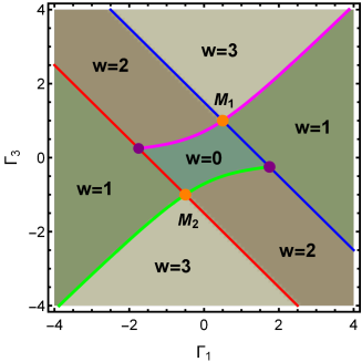
Figure 1: Topological phase diagram. Plotted in the plane $\Gamma_{1}-\Gamma_{3}$ with $\Gamma_{0}=1$, $\Gamma_{2}=0.5$. The gapped phases are identified with integer winding number. These phases are separated by the four critical lines. The HS critical lines are represented in red (for $k_{0}=0$) and blue (for $k_{0}=\pm\pi$). The non-HS critical lines are represented in magenta (for $\pm k_{0}$ in Eq.3) and green (for $\pm k_{0}$ in Eq.4). Among the four multicritical points two are identified with quadratic dispersion (purple dots) and other two are identified with linear dispersion (orange dots) which are labeled $M_{1,2}$.

As the nearest-neighbor couplings are increased the gap closing can also occur at arbitrary points in the Brillouin zone, which are referred to as non-HS points murakami2011gap ; kourtis2017weyl ; molignini2018universal . The distinct gapped phases (i.e. $w=0\leftrightarrow 2$, and $w=1\leftrightarrow 3$) are also separated by non-HS critical points/lines at which the gap closes at non-HS momenta in the Brillouin zone. Moreover, at each point on the non-HS critical lines, the gap closing occurs at a pair of non-HS momenta, as shown in Fig.2(c) and (d). In our model, these points can be obtained for

$$k_{0}=\pm\arccos((-2\Gamma_{2}+\sqrt{4\Gamma_{2}^{2}-16\Gamma_{3}(\Gamma_{1}-\Gamma_{3})})/8\Gamma_{3})$$ (3)

which yield the critical line $\Gamma_{3}=(\Gamma_{1}+\sqrt{\Gamma_{1}^{2}+4\Gamma_{0}(\Gamma_{0}-\Gamma_{2})})/2$ (magenta line in Fig.1), and

$$k_{0}=\pm\arccos((-2\Gamma_{2}-\sqrt{4\Gamma_{2}^{2}-16\Gamma_{3}(\Gamma_{1}-\Gamma_{3})})/8\Gamma_{3})$$ (4)

which yield the critical line $\Gamma_{3}=(\Gamma_{1}-\sqrt{\Gamma_{1}^{2}+4\Gamma_{0}(\Gamma_{0}-\Gamma_{2})})/2$ (green line in Fig.1). Therefore, HS and non-HS critical lines together distinguish the gapped phases with $w=0,1,2,3$ as shown in Fig.1. Note that, the pair of non-HS gap closing points have identical critical properties. Therefore, we address only one point throughout the discussion.

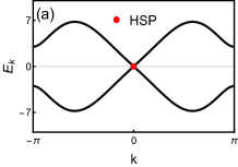
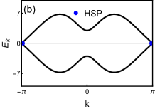
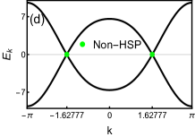
Figure 2: Energy dispersion for HS and non-HS critical points. (a) HS point at $k_{0}=0$ which can be obtained for the values of the parameters satisfying the relation $\Gamma_{3}=-(\Gamma_{0}+\Gamma_{1}+\Gamma_{2})$ (red critical line in Fig.1). (b) HS point at $k_{0}=\pm\pi$ which can be obtained for the values of the parameters satisfying the relation $\Gamma_{3}=(\Gamma_{0}-\Gamma_{1}+\Gamma_{2})$ (blue critical line in Fig.1). (c) Non-HS point at $k_{0}$ in Eq.3 where the values of the parameters satisfy $\Gamma_{3}=(\Gamma_{1}+\sqrt{\Gamma_{1}^{2}+4\Gamma_{0}(\Gamma_{0}-\Gamma_{2})})/2$ (magenta critical line in Fig.1). (d) Non-HS point at $k_{0}$ in Eq.4 where the values of the parameters satisfy $\Gamma_{3}=(\Gamma_{1}-\sqrt{\Gamma_{1}^{2}+4\Gamma_{0}(\Gamma_{0}-\Gamma_{2})})/2$ (green critical line in Fig.1).

Moreover, the model possess four multicritical points at the intersections of HS and non-HS critical lines. Two of them are identified with quadratic dispersion (purple dots in Fig.1) whilst the other two are with linear dispersion (orange dots, named $M_{1}$ and $M_{2}$ in Fig.1). The quadratic multicriticalities are obtained for $\Gamma_{1}=\pm(3\Gamma_{0}+\Gamma_{2})/2$ and linear multicriticalities are obtained for $\Gamma_{1}=\pm\Gamma_{2}$ (here the sign ${}^{\prime}\pm^{\prime}$ represents $M_{1}$ and $M_{2}$ respectively). In our model, each non-HS critical line is separated by the multicritical points into two segments. These two segments can be identified with distinct topologies (discussed later). Moreover, the critical lines manifest as critical regions or critical surfaces in the three-dimensional parameter space. Every point on this critical surface is a gap-closing critical point. Therefore, we refer to the different segments of critical lines as critical phases.

Localized edge modes living at certain criticalities, lead to a unique topological transition along the critical lines between distinct critical phases kumar2021topological ; kumar2021multi . In this work, we aim to identify topological distinct nature among the non-HS critical phases and the topological transition between them. We achieve this in three steps. At first, we develop CRG method to address the non-HS criticality and show that it works in identifying the conventional topological transition between gapped phases (Section.III). Later, we construct the model at non-HS criticality and show topological distinct non-HS critical phases and its edge mode solutions both analytically and numerically (Section.IV). Finally, we reframe the CRG method to work at non-HS criticality in order to capture the unique topological transition between non-HS critical phases (Section.V).

III CRG for topological transition between gapped phases through non-HS quantum criticality

The critical behavior of the system can be captured by a scaling scheme based on the divergence of curvature function at a critical point chen2016scaling . The curvature function can be defined as

$$F(k,\mathbf{\Gamma})=\frac{\chi_{x}\partial_{k}\chi_{y}-\chi_{y}\partial_{k}\chi_{x}}{\chi_{x}^{2}+\chi_{y}^{2}},$$ (5)

whose integral over the Brillouin zone gives the winding number in Eq.2. The scaling involves finding a $\mathbf{\Gamma}^{\prime}$ for every $\mathbf{\Gamma}$ such that $F(k_{0},\mathbf{\Gamma}^{\prime})=F(k_{0}+\delta k,\mathbf{\Gamma})$, where $\delta k$ is small deviation from a HS point $k_{0}$. This procedure gradually reduces the deviation in the curvature function from its fixed point configuration while preserving the topological propertychen2016scaling . Eventually, the scaling scheme yields RG flow in parameter space which enable the identification of critical points, at which the topological transition occurs, along with fixed points.

However, the same scaling scheme does not capture the non-HS critical points, where the peak in the curvature function occur away from HS points and the corresponding $k_{0}$ changes with every $\mathbf{\Gamma}^{\prime}$. Nevertheless, in some cases, the scaling at HS points can reveal the non-HS critical behavior in terms of RG flow lines malard2020scaling ; abdulla2020curvature . Although, this advantage is not universal and is lost when certain conditions to the parameters are imposed in the model kumar2021multi . Therefore, in general, the CRG for HS points fails to capture the non-HS criticalities.

Here we reframe the scaling procedure to obtain an effective scheme which can directly capture the topological transition at non-HS criticality between gapped phases. Similar to the case of HS criticalities, the curvature function shows diverging property by tuning the parameter towards non-HS criticalities as well, i.e. $\mathbf{\Gamma}\rightarrow\mathbf{\Gamma}_{c}$. The momenta at which the diverging peak occurs ($k_{0}$) is a set of non-HS points $k_{0}=\left\{\pm k_{0}^{c},\pm k_{0}^{1},\pm k_{0}^{2},...\right\}$ where $k_{0}^{c}$ is the momentum for $\mathbf{\Gamma}=\mathbf{\Gamma}_{c}$ and the other points are for the parameter values away from the criticality (i.e. $\mathbf{\Gamma}\neq\mathbf{\Gamma}_{c}$). The diverging peak of the curvature function increases as $\mathbf{\Gamma}\rightarrow\mathbf{\Gamma}_{c}$ leading to complete divergence at $\mathbf{\Gamma}=\mathbf{\Gamma}_{c}$ and $k_{0}=\pm k_{0}^{c}$.

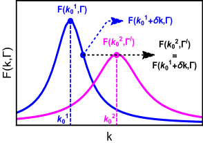
Figure 3: Curvature function in the vicinity of non-HS critical point. As one tune the parameter $\mathbf{\Gamma}$ to $\mathbf{\Gamma^{\prime}}$ away from the critical point, peak of the curvature function $F(k,\mathbf{\Gamma})$ decreases and shits from $k_{0}^{1}$ to $k_{0}^{2}$. This enable one to realize the scaling of the form $F(k_{0}^{2},\mathbf{\Gamma}^{\prime})=F(k_{0}^{1}+\delta k,\mathbf{\Gamma})$.

Moreover, the curvature function flips the sign as the parameters passes through the non-HS critical point

$$\lim_{\mathbf{\Gamma}\rightarrow\mathbf{\Gamma}_{c}^{+}}F(k_{0},\mathbf{\Gamma})=-\lim_{\mathbf{\Gamma}\rightarrow\mathbf{\Gamma}_{c}^{-}}F(k_{0},\mathbf{\Gamma})=\pm\infty.$$ (6)

The curvature function is symmetric around a non-HS point, $F(k_{0}+\delta k,\mathbf{\Gamma})=F(k_{0}-\delta k,\mathbf{\Gamma})$, where $\delta k$ is small deviation from non-HS point $k_{0}$, and by choosing a proper gauge it can be written in terms Ornstein-Zernike form

$$F(k_{0}+\delta k,\mathbf{\Gamma})=\frac{F(k_{0},\mathbf{\Gamma})}{1+\xi^{2}\delta k^{2}},$$ (7)

where $\xi$ is characteristic length scale (inverse of the width of curvature function). This length scale also shows the diverging property on approaching the non-HS critical point. Therefore, one can define the critical exponents for the divergence of curvature function as

$$F(k_{0},\mathbf{\Gamma})\propto|\mathbf{\Gamma}-\mathbf{\Gamma}_{c}|^{-\gamma},\;\;\;\;\;\;\xi\propto|\mathbf{\Gamma}-\mathbf{\Gamma}_{c}|^{-\nu},$$ (8)

where the exponents $\gamma$ and $\nu$ dictates the universality class of non-HS criticalities. For one dimensional systems, these exponents obeys the scaling law $\gamma=\nu$, which is imposed by the conservation of topological invariant chen2017correlation .

The striking similarities in the behavior of curvature function between HS and non-HS criticalities, allows one to reframe the scaling theory purely in terms of non-HS points. Let us consider that as $\mathbf{\Gamma}$ is tuned to $\mathbf{\Gamma}^{\prime}$ the peak develops at $k_{0}^{1}$ and then shifts to $k_{0}^{2}$ respectively, as shown in Fig.3. For this property the scaling can be written as

$$F(k_{0}^{2},\mathbf{\Gamma}^{\prime})=F(k_{0}^{1}+\delta k,\mathbf{\Gamma}).$$ (9)

Expansion of this equation to the leading orders in $\mathbf{\Gamma^{\prime}}$ and $k_{0}^{1}$ gives

$$F(k_{0}^{1},\mathbf{\Gamma})-F(k_{0}^{2},\mathbf{\Gamma})+\delta k\partial_{k}F(k,\mathbf{\Gamma})|_{k=k_{0}^{1}}\\ =(\mathbf{\Gamma}^{\prime}-\mathbf{\Gamma})\partial_{\mathbf{\Gamma}}F(k_{0}^{2},\mathbf{\Gamma})$$ (10)

To obtain the RG equation, without loss of generality, one can choose the parameter values ($\mathbf{\Gamma}$ and $\mathbf{\Gamma}^{\prime}$) in such a way that the non-HS points $k_{0}^{1}$ and $k_{0}^{2}$ have the closest values i.e. $k_{0}^{1}\approxeq k_{0}^{2}$, for which the curvature functions are negligibly different i.e. $F(k_{0}^{1},\mathbf{\Gamma})\approxeq F(k_{0}^{2},\mathbf{\Gamma})$. This approximation yields the generic CRG equation

$$\frac{d\mathbf{\Gamma}}{dl}\approx\frac{\partial_{k}F(k,\mathbf{\Gamma})|_{k=k_{0}}}{\partial_{\mathbf{\Gamma}}F(k_{0},\mathbf{\Gamma})},$$ (11)

where $d\mathbf{\Gamma}=\mathbf{\Gamma}^{\prime}-\mathbf{\Gamma}$ and $dl=\delta k$. The RG flow direction together with the flow rate determines the critical and fixed points in the parameters space chen2018weakly as

Critical point: $$\hskip 5.69046pt\left|\frac{d\mathbf{\Gamma}}{dl}\right|\rightarrow\infty,\text{flow directs away},$$

Stable fixed point: $$\left|\frac{d\mathbf{\Gamma}}{dl}\right|\rightarrow 0,\text{flow directs into},$$

Unstable fixed point: $$\left|\frac{d\mathbf{\Gamma}}{dl}\right|\rightarrow 0,\text{flow directs away}.$$ (12)

Interestingly, the Wannier-state correlation function, obtained from the charge-polarization correlation between Wannier states at different positionschen2017correlation , can be extended to identify the topological transition through non-HS criticality. It can be obtained from the Fourier transform of the curvature function and the substitution of Ornstein-Zernike form. The correlation function can be written as

$$\lambda_{R}=\left\langle R|\hat{r}|0\right\rangle=e^{ik_{0}R}\frac{F(k_{0},\mathbf{\Gamma})}{2\xi}e^{-\frac{R}{\xi}},$$ (13)

where $\hat{r}$ is the position operator for the Wannier states at a distance $R$ from the origin $\ket{0}$, defined as $\ket{R}=\int dke^{ik(\hat{r}-R)}\ket{u_{k}}$ with $\ket{u_{k}}$ being a Bloch state. In Eq.13, $k_{0}$ is the non-HS point and the $\xi$ cab be regarded as correlation length, which coincides with the decay length of the edge modes in topological non-trivial phasechen2017correlation . The correlation function $\lambda_{R}$ decays exponentially near the non-HS critical point and the decay gets slower as we tune towards the criticality with the diverging correlation length $\xi$. This clearly indicate the topological transition through non-HS criticality between gapped phases.

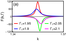
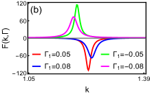
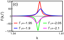
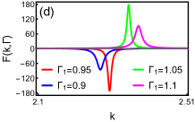
Figure 4: Nature of curvature function in the vicinity of non-HS criticalities i.e. magenta and green critical lines in Fig.1. Fixing the values $\Gamma_{0}$, $\Gamma_{2}$ and $\Gamma_{3}$, the parameter $\Gamma_{1}$ is varied around the critical value $\Gamma_{1}^{c}$. For all the plots $\Gamma_{0}=1$ and $\Gamma_{2}=0.5$. (a) For $\Gamma_{3}=2.2$ and $\Gamma_{1}^{c}=2$. It is a critical point on the magenta line between the phases $w=3$ and $w=1$. (b) For $\Gamma_{3}=0.7$ and $\Gamma_{1}^{c}=0$. It is a critical point on the magenta line between the phases $w=2$ and $w=0$. (c) For $\Gamma_{3}=-2.2$ and $\Gamma_{1}^{c}=-2$. It is a critical point on the green line between the phases $w=3$ and $w=1$. (d) For $\Gamma_{3}=-0.36$ and $\Gamma_{1}^{c}=1$. It is a critical point on the green line between the phases $w=2$ and $w=0$.

III.1 Curvature function and critical exponents

The curvature function of the model in Eq.1 can be obtained using the pseudo-spin vectors as

$$F(k,\mathbf{\Gamma}) =\frac{\chi_{y}\partial_{k}\chi_{x}-\chi_{x}\partial_{k}\chi_{y}}{\chi_{x}^{2}+\chi_{y}^{2}}$$ (14)

$$=\frac{A+B\cos(k)+C\cos(2k)+D\cos(3k)}{A^{\prime}+B^{\prime}\cos(k)+C^{\prime}\cos(2k)+D^{\prime}\cos(3k)},$$

where $A=\Gamma_{1}^{2}+2\Gamma_{2}^{2}+3\Gamma_{3}^{2}$, $A^{\prime}=\Gamma_{0}^{2}+\Gamma_{1}^{2}+\Gamma_{2}^{2}+\Gamma_{3}^{2}$, $B=\Gamma_{0}\Gamma_{1}+3\Gamma_{1}\Gamma_{2}+5\Gamma_{2}\Gamma_{3}$, $B^{\prime}=2(\Gamma_{0}\Gamma_{1}+\Gamma_{1}\Gamma_{2}+\Gamma_{2}\Gamma_{3})$, $C=2\Gamma_{0}\Gamma_{2}+4\Gamma_{1}\Gamma_{3}$, $C^{\prime}=2(\Gamma_{0}\Gamma_{2}+\Gamma_{1}\Gamma_{3})$, $D=3\Gamma_{0}\Gamma_{3}$ and $D^{\prime}=2\Gamma_{0}\Gamma_{3}$.    In Fig.4, we show the nature of curvature function in the vicinity of the non-HS criticalities, $\Gamma_{3}=(\Gamma_{1}\pm\sqrt{\Gamma_{1}^{2}+4\Gamma_{0}(\Gamma_{0}-\Gamma_{2})})/2$ (i.e. magenta and green lines in Fig.1). Setting $\Gamma_{0}=1$ and $\Gamma_{2}=0.5$ we tune $\Gamma_{1}$ towards its critical values (say $\Gamma_{1}^{c}$) for a fixed value of $\Gamma_{3}$. For the non-HS critical point between the gapped phases $w=1$ and $w=3$, $\Gamma_{1}^{c}=\pm 2$ and $\Gamma_{3}=\pm 2.2$ respectively for magenta and green criticalities. For $w=0$ and $w=2$, $\Gamma_{1}^{c}=0$ and $\Gamma_{3}=0.7$ for magenta and $\Gamma_{1}=1$ and $\Gamma_{3}=-0.36$ for green criticalities. Fixing $\Gamma_{3}$, we vary $\Gamma_{1}$ around the critical point, as shown in Fig.4.

As one tune the parameter $\Gamma_{1}$ towards its critical value $\Gamma_{1}^{c}$, diverging peak occurs at non-HS points $k_{0}$, which shifts each time the $\Gamma_{1}$ is varied. The peak becomes prominent as we approach $\Gamma_{1}=\Gamma_{1}^{c}$ and flips the sign as we tune further across the critical point. These properties of curvature function can be observed for both non-HS criticalities. Note that, the same nature of curvature function can also be observed at the negative pair of non-HS point. Therefore, the divergence and flipping of curvature function can be considered as an efficient qualitative observation to identify the topological transition through non-HS criticalities.

The behavior of the curvature function can be quantified in terms of critical exponents $\gamma$ and $\nu$ as defined in Eq.8, which captures the divergences in the height $F(k_{0},\mathbf{\Gamma})$ and inverse of the width $\xi$ of curvature function. The values of these exponents can be obtained by numerical fitting of the curvature function with

$$F_{fitting}=c+\frac{F(k_{0},\mathbf{\Gamma})}{1+\xi^{2}(k-k_{0})^{2}}$$ (15)

where $c$ is an arbitrary constant. The fitting is done by varying $\mathbf{\Gamma}$ in the vicinity of the non-HS critical points with corresponding $k_{0}$ values. The data points collected for $|F(k_{0},\mathbf{\Gamma})|$ and $\xi$ can then be fitted again with Eq.8 to extract the exponents. Fig.5 demonstrates this process and shows the exponent values on approaching the non-HS critical points from either sides (represented as $\gamma_{+/-}$ and $\nu_{+/-}$). The data points are collected by fixing the parameters $\Gamma_{0}$, $\Gamma_{2}$ and $\Gamma_{3}$ and varying $\Gamma_{1}$ by $\delta\Gamma_{1}$ ($\delta\Gamma_{1}=|\Gamma_{1}-\Gamma_{1}^{c}|$) on either sides of the critical points.

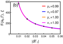
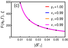
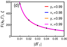
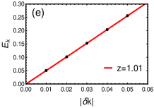
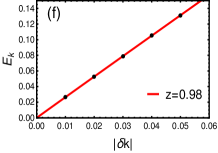
Figure 5: Critical exponents for non-HS quantum criticalities. For all the plots $\Gamma_{0}=1$ and $\Gamma_{2}=0.5$. (a) For $\Gamma_{3}=2.2$ and $\Gamma_{1}^{c}=2$. (b) For $\Gamma_{3}=0.7$ and $\Gamma_{1}^{c}=0$. (c) For $\Gamma_{3}=-2.2$ and $\Gamma_{1}^{c}=-2$. (d) For $\Gamma_{3}=-0.7$ and $\Gamma_{1}^{c}=0$. For all the cases exponents are found to be $\gamma=\gamma_{+/-}\approx 1$ and $\nu=\nu_{+/-}\approx 1$. (e) Dynamical critical exponent for a critical point between the gapped phases $w=1$ and $w=3$. (f) Dynamical critical exponent for a critical point between the gapped phases $w=0$ and $w=2$.

The critical exponents can also be calculated analytically by expanding the pseudo-spin vector $\boldsymbol{\chi}(k)$ around non-HS point $k_{0}$ and recasting the curvature function in the Ornstein-Zernike form. The expansion upto first order, $\boldsymbol{\chi}(k)|_{k=k_{0}}\approx\boldsymbol{\chi}(k_{0})+\partial_{k}\boldsymbol{\chi}(k_{0})\delta k$, for the non-HS points $k_{0}=\arccos((-2\Gamma_{2}\pm\sqrt{4\Gamma_{2}^{2}-16\Gamma_{3}(\Gamma_{1}-\Gamma_{3})})/8\Gamma_{3})$ yields (the sign ‘$\pm$’ represents the magenta and green criticalities respectively)

$$\chi_{x}\approx\delta\mathbf{\Gamma}+A\delta k\;\;\;\quad\text{and}\quad\;\;\;\chi_{y}\approx B\delta k,$$ (16)

where

$$\delta\mathbf{\Gamma}=\Gamma_{0}-\Gamma_{2}/2\mp(1/2)\alpha$$

$$A=\frac{(4\Gamma_{1}\Gamma_{3}-\Gamma_{2}^{2}\pm\Gamma_{2}\alpha)\sqrt{2\Gamma_{3}(\Gamma_{1}+3\Gamma_{3}-\Gamma_{2}^{2}\pm\Gamma_{2}\alpha)}}{4\sqrt{2}\Gamma_{3}^{2}}$$

$$B=\frac{-\Gamma_{2}^{3}+4\Gamma_{2}\Gamma_{3}(\Gamma_{1}-\Gamma_{3})\pm\Gamma_{2}^{2}\alpha\mp 2\Gamma_{3}(\Gamma_{1}+3\Gamma_{3}\alpha)}{4\Gamma_{3}^{2}}$$ (17)

with $\alpha=\sqrt{\Gamma_{2}^{2}+4\Gamma_{3}(\Gamma_{3}-\Gamma_{1})}$. Therefore the curvature function in Eq.14 can be recasted as

$$F(k,\delta\mathbf{\Gamma}) =\frac{-B/\delta\mathbf{\Gamma}}{1+\left(\frac{2A}{\delta\mathbf{\Gamma}}\right)\delta k+\left(\frac{A^{2}+B^{2}}{\delta\mathbf{\Gamma}^{2}}\right)\delta k^{2}}$$

$$=\frac{F(k_{0},\delta\mathbf{\Gamma})}{1+\xi\delta k+\xi^{2}\delta k^{2}}$$ (18)

Note that, the term $\xi^{2}$ is dominant as it diverges more quickly than $\xi$, therefore, one can obtain the Ornstein-Zernike form using only the leading term in the denominator. The critical exponents $\gamma$ and $\nu$ are

$$F(k_{0},\delta\mathbf{\Gamma})=-B\delta\mathbf{\Gamma}^{-1}\implies\gamma=1$$ (19)

$$\xi=\sqrt{(A^{2}+B^{2})}\delta\mathbf{\Gamma}^{-1}\implies\nu=1.$$ (20)

This clearly demonstrate that, analytical and numerical values of critical exponents agree each other. Therefore, the exponents $\gamma=\nu=1$ for both the non-HS criticalities and they obey the scaling law $\gamma=\nu$ for 1D systems.

Moreover, the vanishing energy scale of the gap function $\Delta$, defines a gap exponent

$$\Delta\propto|\mathbf{\Gamma}-\mathbf{\Gamma}_{c}|^{y},$$ (21)

where $y=z\nu$, which is dynamical scaling law jalal2016topological with $z$ the dynamical critical exponent malard2020scaling ; rufo2019multicritical . The $z$ dictates the nature of the spectra near the gap closing momenta $k_{0}$, i.e. $E_{k}\propto k^{z}$. It can be calculated numerically using curve fitting method similar to the previous case. This procedure results in the Fig.5(e) and (f), which yields $z=1$ for both the non-HS criticalities. The gap exponent can be obtained as $y=z\nu=1$. The critical exponents defines the universality class of the topological transition through both non-HS quantum criticalities between gapped phases. Therefore, both the non-HS criticalities share the same universality class $(\gamma,\nu,z)=(1,1,1)$.

III.2 Curvature function renormalization group and correlation function

In this section, we perform CRG to the model in Eq.1 and obtain RG equations which essentially captures the topological transition between gapped phases through non-HS criticalities. The RG equations in terms of the parameters for the non-HS points can be constructed from Eq.11. For the non-HS point $k_{0}=\arccos((-2\Gamma_{2}+\sqrt{4\Gamma_{2}^{2}-16\Gamma_{3}(\Gamma_{1}-\Gamma_{3})})/8\Gamma_{3})$ (corresponds to magenta line in Fig.1), the RG equations for $\Gamma_{1}$ and $\Gamma_{3}$ ($\Gamma_{0}=1$ and $\Gamma_{2}=0.5$) can be obtained as

$$\dfrac{d\Gamma_{1}}{dl}=\frac{\alpha\sqrt{\alpha_{1}}\Lambda_{1}(\Gamma_{0},\Gamma_{1},\Gamma_{2},\Gamma_{3})}{2\sqrt{2}\Lambda_{2}(\Gamma_{0},\Gamma_{1},\Gamma_{2},\Gamma_{3})}$$ (22)

$$\dfrac{d\Gamma_{3}}{dl}=\frac{\Gamma_{3}^{2}\alpha\sqrt{\alpha_{1}}\Lambda_{1}(\Gamma_{0},\Gamma_{1},\Gamma_{2},\Gamma_{3})}{2\sqrt{2}\Lambda_{2}^{\prime}(\Gamma_{0},\Gamma_{1},\Gamma_{2},\Gamma_{3})}$$ (23)

Similarly, for the non-HS point $k_{0}=\arccos((-2\Gamma_{2}-\sqrt{4\Gamma_{2}^{2}-16\Gamma_{3}(\Gamma_{1}-\Gamma_{3})})/8\Gamma_{3})$ (corresponds to green line in Fig.1) we obtain

$$\dfrac{d\Gamma_{1}}{dl}=-\frac{\alpha\sqrt{\alpha_{1}}\Lambda_{3}(\Gamma_{0},\Gamma_{1},\Gamma_{2},\Gamma_{3})}{\sqrt{2}\Gamma_{3}^{2}\Lambda_{4}(\Gamma_{0},\Gamma_{1},\Gamma_{2},\Gamma_{3})}$$ (24)

$$\dfrac{d\Gamma_{3}}{dl}=-\frac{\alpha\sqrt{\alpha_{1}}\Lambda_{3}(\Gamma_{0},\Gamma_{1},\Gamma_{2},\Gamma_{3})}{\sqrt{2}\Lambda_{4}^{\prime}(\Gamma_{0},\Gamma_{1},\Gamma_{2},\Gamma_{3})}$$ (25)

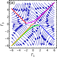
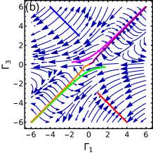
Figure 6: CRG flow diagram. Plotted for $\Gamma_{0}=1$ and $\Gamma_{2}=0.5$. (a) RG flow for magenta criticality. (b) RG flow for green criticality. The magenta and green criticalities manifests as stable and unstable fixed points respectively. These lines coincides with the fixed lines represented in orange and purple. The HS lines, represented as red and blue lines, are partially recognised by the RG flow as stable and unstable fixed lines respectively.

where $\alpha=\sqrt{\Gamma_{2}^{2}+4\Gamma_{3}(-\Gamma_{1}+\Gamma_{3})}$ and $\alpha_{1}=\sqrt{(2\Gamma_{3}(\Gamma_{1}+3\Gamma_{3})-\Gamma_{2}^{2}+\Gamma_{2}\alpha)}/\Gamma_{3}$ (see supplementary material for detailed form of $\Lambda$s). The non-HS criticalities can be identified from the RG flow in the $\Gamma_{1}-\Gamma_{3}$ plane. In general, the RG flow rate and the direction enables the identification the critical and fixed points (stable and unstable) in the parameter space chen2018weakly , as explained in Eq.12. However, in this case, the RG flow exhibits an anomalous behavior that both the non-HS criticalities simultaneously satisfy the fixed and critical line conditions. In other words, the non-HS criticalities drives both numerator and denominator of the RG equations to zero individually. This is due to the overlap of critical and fixed lines in the flow diagram.

The fixed lines can be obtained as $\Gamma_{3}=1/2(\Gamma_{1}+\sqrt{\Gamma_{1}^{2}-\Gamma_{2}^{2}})$ which defines stable fixed points and $\Gamma_{3}=1/2(\Gamma_{1}-\sqrt{\Gamma_{1}^{2}-\Gamma_{2}^{2}})$ which defines unstable fixed points (represented as purple and orange lines respectively in Fig.6). These lines coincide with the non-HS critical lines for higher values of parameters i.e. $|\Gamma_{1}|$ and $|\Gamma_{2}|$. This results in the manifestation of the magenta critical lines as stable fixed line and green critical line as unstable fixed line, as shown in Fig.6(a,b). The manifestation of the critical lines as fixed lines can be found in agreement with the observations made in Ref.malard2020scaling ; abdulla2020curvature .

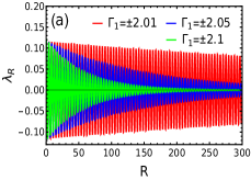
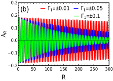
Figure 7: Wannier state correlation function. The parameter values $\Gamma_{0}=1$ and $\Gamma_{2}=0.5$ are fixed. (a) Represents $\lambda_{R}$ in the vicinity of a critical point between the gapped phases $w=1$ and $w=3$. For the magenta line we choose $\Gamma_{1}^{c}=2$ and $\Gamma_{3}=2.2$ and for the green line $\Gamma_{1}^{c}=-2$ and $\Gamma_{3}=-2.2$. (b) Represents $\lambda_{R}$ in the vicinity of a critical point between $w=0$ and $w=2$. For the magenta line $\Gamma_{1}^{c}=0$ and $\Gamma_{3}=0.7$ and green line $\Gamma_{1}^{c}=0$ and $\Gamma_{3}=-0.7$.

Apart from this, interestingly the CRG constructed for non-HS criticalities partially captures the HS criticalities which are also manifested as fixed lines in the flow diagram. As shown in Fig.6 the HS criticalities $\Gamma_{3}=\mp(\Gamma_{0}\pm\Gamma_{1}+\Gamma_{2})$ (the red and blue lines) appear as the stable and unstable fixed points respectively. Therefore, the CRG developed for non-HS criticalities is efficient in detecting the corresponding topological transition between gapped phases and also partially captures the HS topological transitions.

The Wannier state correlation function $\lambda_{R}$ defined in Eq.13, clearly identify the topological transitions at the non-HS criticalities of the model. Fig.7 shows the profile of the correlation function in the vicinity of both the non-HS criticalities. For $k_{0}=\arccos((-2\Gamma_{2}\pm\sqrt{4\Gamma_{2}^{2}-16\Gamma_{3}(\Gamma_{1}-\Gamma_{3})})/8\Gamma_{3})$, Eq.13 yields highly oscillatory decay in $\lambda_{R}$ in the vicinity of the critical points $\Gamma_{1}^{c}=\pm 2$ and $\Gamma_{1}^{c}=0$. As the parameter $\Gamma_{1}$ is tuned towards its critical value the decay in $\lambda_{R}$ slow down leading to the divergence in the length scale $\xi$. This is the typical behavior of the Wannier state correlation function for the topological transitions.

IV Topological phase transition between non-HS critical phases through multicriticality

In this section, we investigate the existence of edge modes at non-HS critical phases and explore the possible topological transition between non-HS critical phases through multicritical points. To achieve this, at first, we construct the model at criticality using the near-critical approach kumar2021topological in which the Hamiltonian can be considered critical only in parameter space i.e. $\mathcal{H}(\mathbf{\Gamma}_{c},k)$ with $k=k_{0}+\Delta k$ where $\Delta k<<2\pi$, to avoid the singularity at exact critical point. This method has been efficiently used to study the HS criticalities kumar2021topological and here we show that it is also effective to address the non-HS criticalities.

To obtain $\mathcal{H}(\mathbf{\Gamma}_{c},k)$, we plug the non-HS critical line expression for $\Gamma_{3}$ into the pseudospin vectors in Eq.1. This yields $\chi_{x}(k)=\Gamma_{0}+\Gamma_{1}\cos k+\Gamma_{2}\cos 2k+(\Gamma_{1}\pm\sqrt{\Gamma_{1}^{2}+4\Gamma_{0}(\Gamma_{0}-\Gamma_{2})})/2\cos 3k,$ and $\chi_{y}(k)=\Gamma_{1}\sin k+\Gamma_{2}\sin 2k+(\Gamma_{1}\pm\sqrt{\Gamma_{1}^{2}+4\Gamma_{0}(\Gamma_{0}-\Gamma_{2})})/2\sin 3k$. The corresponding dispersion vanishes at multicritical points. Among the four multicritical points only the points with linear dispersion ($M_{1,2}$ in Fig.1) separates the distinct non-HS critical phases, as schematically shown in Fig.8. Therefore, we study only $M_{1,2}$, which can be obtained for the momenta

$$k_{0}^{mc}=\pi,\\ \pm\arccos[\frac{-2\Gamma_{2}+\sqrt{-8(\Gamma_{1}+\frac{1}{2}(-\Gamma_{1}-\alpha))(\Gamma_{1}+\alpha+4\Gamma_{2}^{2})}}{4(\Gamma_{1}+\alpha)}]$$ (26)

for $M_{1}$ (multicritical point on the magenta line) and

$$k_{0}^{mc}=0,\\ \pm\arccos[\frac{-2\Gamma_{2}-\sqrt{-8(\Gamma_{1}+\frac{1}{2}(-\Gamma_{1}+\alpha))(\Gamma_{1}-\alpha+4\Gamma_{2}^{2})}}{4(\Gamma_{1}+\alpha)}]$$ (27)

for $M_{2}$ (multicritical point on the green line). Here $\alpha=\sqrt{\Gamma_{1}^{2}+4\Gamma_{0}(\Gamma_{0}-\Gamma_{2})}$. At $M_{1,2}$ the gap closing occurs at three points in the Brillouin zone. One of them is HS point and the other two are non-HS points. This is due to the fact that $M_{1,2}$ are the intersection points of non-HS and HS critical lines (see Fig.1).

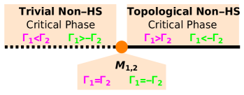
Figure 8: Schematic representation of non-HS criticalities i.e. magenta and green lines in Fig.1. The trivial and non-trivial phases are represented as dashed and solid lines respectively and are separated by multicritical points $M_{1,2}$. For the magenta line $\Gamma_{1}<\Gamma_{2}$ ($\Gamma_{1}>\Gamma_{2}$) represents trivial (non-trivial) critical phase. For the green line $\Gamma_{1}>-\Gamma_{2}$ ($\Gamma_{1}<-\Gamma_{2}$) represents trivial (non-trivial) critical phase. The transition between the trivial and non-trivial phases occur at $\Gamma_{1}=\pm\Gamma_{2}$ on the magenta and green lines respectively.

Now driving the parameters towards the multicritical point involves both $\mathbf{\Gamma}_{c}\rightarrow\mathbf{\Gamma}_{mc}$ and $k\rightarrow k_{0}^{mc}$. In the following subsections we show topological trivial and non-trivial characters of the non-HS critical phases.

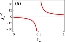
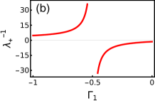
Figure 9: Decay length of edge modes at non-HS criticalities. The parameters $\Gamma_{0}=1$ and $\Gamma_{2}=0.5$ are fixed. (a) On the magenta line. The decay length $\lambda^{-1}_{+}$ can be found to be positive (negative) at non-trivial (trivial) critical phase $\Gamma_{1}>0.5$ ($\Gamma_{1}<0.5$). (b) On the green line. The decay length $\lambda^{-1}_{+}$ can be found positive (negative) at non-trivial (trivial) critical phase $\Gamma_{1}<-0.5$ ($\Gamma_{1}>-0.5$).

IV.1 Decay length of edge modes at non-HS criticalities

To enable the identification of the trivial and topological non-HS critical phases, we calculate the edge mode decay length using the Dirac equation shen2011topological ; lu2011non ; jackiw1976solitons ; verresen2020topology ; kumar2021topological at non-HS criticalities. The multicritical points are the phase boundaries, between distinct non-HS critical phases, at which the gap closes for $k_{0}^{mc}$. We expand the Hamiltonian defined at criticality around $k_{0}^{mc}=\pi,0$ (for magenta and green criticalities respectively) to obtain

$$\mathcal{H}(k)=(m+\epsilon_{1}k^{2})\sigma_{x}+(\epsilon_{2}k)\sigma_{y}$$ (28)

where $m=\Gamma_{0}\mp 3\Gamma_{1}/2-(1/2)\alpha+\Gamma_{2}$, $\epsilon_{1}=\pm\Gamma_{1}+9/2(\Gamma_{1}+\alpha)-4\Gamma_{2}$ and $\epsilon_{2}=\mp 5\Gamma_{1}/2-(3/2)\alpha+2\Gamma_{2}$ with $\alpha=\sqrt{\Gamma_{1}^{2}+4\Gamma_{0}(\Gamma_{0}-\Gamma_{2})}$ (the sign ‘$\pm$’ are for magenta and green lines respectively). The zero energy solution in real space $\mathcal{H}(-i\partial_{x})\psi(x)=0$ (with $\hbar=1$) can be obtained by multiplying $\sigma_{y}$ from right hand side. This implies the wavefunction $\psi(x)=\rho_{\eta}\phi(x)$ is an eigenstate of $\sigma_{z}\rho_{\eta}=\eta\rho_{\eta}$. Using the trial wavefunction $\phi(x)\propto e^{-x\lambda}$ we get

$$-\eta\epsilon_{1}\lambda^{2}+\epsilon_{2}\lambda+\eta m=0$$ (29)

where $\lambda$ is the inverse of the decay length which can be obtained as

$$\lambda_{+}=\frac{m}{\eta\epsilon_{2}}$$ (30)

with $\eta=sign(\epsilon_{2})$. The decay length remain positive for $\Gamma_{1}>\Gamma_{2}$ and negative for $\Gamma_{1}<\Gamma_{2}$ on the magenta line. This means that the critical phase $\Gamma_{1}>\Gamma_{2}$ is the topological phase with the edge modes and $\Gamma_{1}<\Gamma_{2}$ is the trivial critical phase with no edge modes. Similarly, on the green line, $\Gamma_{1}<-\Gamma_{2}$ has positive decay length and is non-trivial critical phase with edge mode while $\Gamma_{1}>-\Gamma_{2}$ is trivial critical phase with no edge modes. The term $m$ plays the role of mass and is zero at the multicritical points $\Gamma_{1}=\pm\Gamma_{2}$. Therefore, as $m\rightarrow 0$ the decay length diverges, as shown in Fig.9, implying the delocalization of the edge modes into the bulk. This clearly indicates that the multicritical points are the topological phase transition points between the distinct non-HS critical phases.

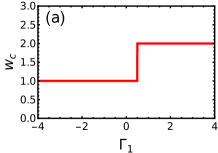
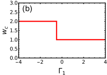
Figure 10: Winding number at non-HS criticalities. The parameters $\Gamma_{0}=1$ and $\Gamma_{2}=0.5$ are fixed. (a) On the magenta line. For trivial phase, $\Gamma_{1}<0.5$, winding number $w_{c}=1$ and for non-trivial phase $\Gamma_{1}>0.5$ the winding number $w_{c}=2$. Transition occurs at the multicritical point $M_{1}$ at $\Gamma_{1}=0.5$. (b) On the green line. For trivial phase, $\Gamma_{1}>-0.5$, winding number $w_{c}=1$ and for non-trivial phase $\Gamma_{1}<-0.5$ the winding number $w_{c}=2$. Transition occurs at the multicritical point $M_{2}$ at $\Gamma_{1}=-0.5$.

IV.2 Winding number at non-HS criticalities

Topological trivial and non-trivial characters of non-HS critical phase can also be identified using winding numbers. The winding number is a topological invariant number which quantify the edge excitations with gapped bulk, i.e. the bulk-boundary correspondence kitaev2001unpaired ; kane2005quantum . As shown in Eq.2, it is defined as the integral of the curvature function over the Brillouin zone which yields integer values $\mathbb{Z}$, and it features a quantized jump at the topological phase transition point hasan2010colloquium . However, the definition in Eq.2 fails at the transition point due to the divergence of the integrand (curvature function). Therefore, in order to quantify the edge modes at criticality one has to exclude the singular point and can write verresen2020topology ; kumar2021topological

$$w_{c}=\frac{1}{2\pi}\lim_{\delta\rightarrow 0}\oint\limits_{|k-k_{0}|>\delta}F(k,\mathbf{\Gamma}_{c})dk.$$ (31)

This defines the winding number at criticality and dictates the fractional values $(\mathbb{Z}/2)$ for HS critical phases verresen2020topology . The quantized jump of the fractional winding number at the transition points indicate the topological transition between HS critical phases. The winding number at non-HS criticalities can also be obtained from Eq.31. In this case, one has to avoid two singular point in the set $k_{0}$, which yields $w_{c}$ integer values, as shown in Fig.10. As each gap closing point can contribute a factor of $(1/2)$, the winding number at the trivial non-HS critical phase is $w_{c}=1$. The non-trivial critical phase with one edge mode is assigned with winding number $w_{c}=2$. Fig.10 shows the topological transition between non-HS critical phases through multicritical point at magenta and green lines.

Based on these observations one can argue that the bulk-boundary correspondence can be realised by identifying the difference between the winding numbers of topological non-trivial and trivial phases (either gapped or critical).

$$\delta w=w^{non-trivial}-w^{trivial},$$ (32)

where $\delta w$ will be non-zero integer and counts the number of edge modes in the corresponding non-trivial phase. In the case of gapped phases, Eq.32 looks trivial as the winding number for a trivial phase $w^{trivial}=0$. However, for the critical phases it provides proper physical picture as it correctly counts the edge modes at the non-trivial critical phase. In case of HS criticality the trivial winding number is $w_{c}^{trivial}=1/2$ and non-trivial winding number is $w_{c}^{non-trivial}=\mathbb{Z}/2$ (where $\mathbb{Z}$ is non-zero integer) verresen2020topology ; kumar2021topological . Therefore, the number of edge modes at the non-trivial HS critical phase is $\delta w_{c}=w_{c}^{non-trivial}-w_{c}^{trivial}=\mathbb{Z}$, this can be found in agreement with Ref kumar2021topological .

In the case of non-HS criticalities, there exists two gap closing points in the momentum space. Therefore, the trivial winding number itself turns out to be an integer (as each gap closing point contributes a factor of $1/2$). The trivial non-HS critical phase is now identified with $w_{c}=1$ and a non-trivial non-HS critical phase is with $w_{c}=\mathbb{Z}$ (where $\mathbb{Z}\geq 2$). In order to obtain correct number of edge modes at the non-trivial critical phase, one has to identify the difference $\delta w_{c}=w_{c}^{non-trivial}-w_{c}^{trivial}=\mathbb{Z}-1$. In our model the non-trivial non-HS critical phases are identified with $w_{c}^{non-trivial}=2$ (see Fig.10) for both the criticalities. Therefore, the proper number of edge modes at these phases can be obtained to be $\delta w_{c}=1$.

The analytical results of winding number and decay length of edge modes at criticality are found to be in agreement with the edge mode solutions obtained numerically under open boundary condition (we refer to supplementary material for the detailed discussion).

V CRG for topological transition between non-HS critical phases

Scaling theory for the topological transition at non-HS critical point between gapped phases is developed in Section.III. Here we reframe this scaling scheme in order to capture the topological transition between non-HS critical phases. This is possible based on the fact that the curvature function defined at criticality using near-critical approach inherits the diverging property. Divergence occurs at the momentum $k_{0}^{mc}$ as one tunes the parameter $\mathbf{\Gamma}_{c}\rightarrow\mathbf{\Gamma}_{mc}$. The diverging peak flips sign as the parameters tuned across the multicritical points

$$\lim_{\mathbf{\Gamma}_{c}\rightarrow\mathbf{\Gamma}_{mc}^{+}}F(k_{0}^{mc},\mathbf{\Gamma}_{c})=-\lim_{\mathbf{\Gamma}_{c}\rightarrow\mathbf{\Gamma}_{mc}^{-}}F(k_{0}^{mc},\mathbf{\Gamma}_{c})=\pm\infty.$$ (33)

The curvature function at criticality is also symmetric and acquires the Ornstein-Zernike form

$$F(k_{0}^{mc}+\delta k,\mathbf{\Gamma}_{c})=\frac{F(k_{0}^{mc},\mathbf{\Gamma}_{c})}{1+\xi_{c}^{2}\delta k^{2}},$$ (34)

where $\xi_{c}$ is the characteristic length scale at criticality. Corresponding critical exponents can be obtained as

$$F(k_{0}^{mc},\mathbf{\Gamma}_{c})\propto|\mathbf{\Gamma}_{c}-\mathbf{\Gamma}_{mc}|^{-\gamma},\;\;\;\;\;\;\xi_{c}\propto|\mathbf{\Gamma}_{c}-\mathbf{\Gamma}_{mc}|^{-\nu}.$$ (35)

In order to construct a scaling scheme similar to the gapped case, we consider the non-HS points of $k_{0}^{mc}$, which effectively captures the scaling at multicritical points (a reverse technique is used in Ref  malard2020scaling , where scaling at HS points identify the non-HS criticalities). The scaling now can be recasted as

$$F(k^{mc}_{02},\mathbf{\Gamma^{\prime}}_{c})=F(k^{mc}_{01}+\delta k,\mathbf{\Gamma}_{c}).$$ (36)

Considering the same approximation employed in the case of gapped phases (Section.III), the generic RG equation at non-HS criticality can be obtained as

$$\frac{d\mathbf{\Gamma}_{c}}{dl}\approx\frac{\partial_{k}F(k,\mathbf{\Gamma}_{c})|_{k=k^{mc}_{0}}}{\partial_{\mathbf{\Gamma}_{c}}F(k^{mc}_{0},\mathbf{\Gamma}_{c})},$$ (37)

where $d\mathbf{\Gamma}_{c}=\mathbf{\Gamma^{\prime}}_{c}-\mathbf{\Gamma}_{c}$ and $dl=\delta k$ (with $\delta k$ being small deviation away from $k^{mc}_{0}$). The RG flow lines identify the topological transition between non-HS critical phases.

The correlation function in terms of Wannier state representation can also be written at non-HS criticalities to characterize the topological transition. At criticality one can write

$$\lambda^{c}_{R}=\frac{e^{ik_{0}^{mc}R}}{2\xi_{c}}F(k_{0}^{mc},\mathbf{\Gamma}_{c})e^{R/\xi_{c}},$$ (38)

where $\xi_{c}$ is the correlation length. The correlation function $\lambda^{c}_{R}$ decays as the parameters tune towards the multicritical point. The decay rate decreases near the point and gets sharper as we tune away from the point. This typical behavior of $\lambda^{c}_{R}$ confirms the topological transition at multicritical points between non-HS critical phases.

V.1 Curvature function and critical exponents

Curvature function at non-HS criticalities can be written using the components $\chi_{x}(k)=\Gamma_{0}+\Gamma_{1}\cos k+\Gamma_{2}\cos 2k+(\Gamma_{1}\pm\sqrt{\Gamma_{1}^{2}+4\Gamma_{0}(\Gamma_{0}-\Gamma_{2})})/2\cos 3k,$ and $\chi_{y}(k)=\Gamma_{1}\sin k+\Gamma_{2}\sin 2k+(\Gamma_{1}\pm\sqrt{\Gamma_{1}^{2}+4\Gamma_{0}(\Gamma_{0}-\Gamma_{2})})/2\sin 3k$.

$$F(k,\mathbf{\Gamma}_{c})=\frac{A+B\cos(k)+C\cos(2k)}{2D^{2}+E^{2}},$$ (39)

where $A=6\Gamma_{0}^{2}+\Gamma_{1}(3\Gamma_{1}\pm\alpha)-8\Gamma_{0}\Gamma_{2}+4\Gamma_{2}^{2}$, $B=-2\Gamma_{0}\Gamma_{1}+\Gamma_{2}(\pm 7\Gamma_{1}+\alpha)$, $C=6\Gamma_{0}(\Gamma_{2}-\Gamma_{0})$, $D=(\Gamma_{1}+\Gamma_{2}\cos(k))^{2}$ and $E=(\Gamma_{2}-2\Gamma_{0})^{2}\sin(k)^{2}$ with $\alpha=\sqrt{\Gamma_{1}^{2}+4\Gamma_{0}(\Gamma_{0}-\Gamma_{2})}$. The diverging peak of the curvature function can be observed at $k_{0}^{mc}$, as one tune the parameters $\mathbf{\Gamma}_{c}$ towards $\mathbf{\Gamma}_{mc}$. The peaks at non-HS $k_{0}^{mc}$ points are shown in Fig.11. The diverging peak flips the sign (similar to the case of gapped phases) as we tune across the multicritical points ($M_{1,2}$) signaling the topological transition between non-HS critical phases. In Fig.11(a), curvature function in the vicinity of the multicritical point $M_{1}$, i.e. $\Gamma_{1}=0.5$ on the magenta line is shown. In Fig.11(b), multicritical point $M_{2}$, i.e. $\Gamma_{1}=-0.5$ on the green line is shown. Therefore, both the non-HS criticalities shows the similar behavior of curvature function at criticality. The multicritical points $M_{1,2}$ are the topological phase transition points between non-HS critical phases.

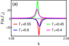
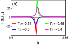
Figure 11: Curvature function at non-HS criticalities. Plotted for $\Gamma_{0}=1$ and $\Gamma_{2}=0.5$. (a) Curvature function at magenta line in the vicinity of the multicritical point $\Gamma_{1}=0.5$ ($M_{1}$) for one of the non-HS $k_{0}^{mc}$. (b) Curvature function at green line in the vicinity of the multicritical point $\Gamma_{1}=-0.5$ ($M_{2}$) for one of the non-HS $k_{0}^{mc}$.

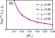
Figure 12: Critical exponents for multicritical points. Plotted for $\Gamma_{0}=1$ and $\Gamma_{2}=0.5$. (a) For $\Gamma_{1}=0.5$ ($M_{1}$). (b) For $\Gamma_{1}=-0.5$ ($M_{2}$). The exponents are found to be $\gamma\approx\nu\approx 1$ for both the multicritical points.

The critical exponents of the curvature function at criticality near the multicritical points can be obtained from Eq.35. The Ornstein-Zernike form of the curvature function in the vicinity of the multicritical points allows one to extract the exponent values numerically using the fitting equation

$$F_{fitting}=c+\frac{F(k_{0}^{mc},\mathbf{\Gamma}_{c})}{1+\xi_{c}^{2}(k-k_{0}^{mc})^{2}}$$ (40)

Fig.12 shows that, one can extract the exponents values as $\gamma\approx\nu\approx 1$ for both the multicritical points $M_{1,2}$.

The exponents can also be evaluated analytically similar to the case of gapped phases. Expansion of the components $\chi_{x,y}$ around $k_{0}^{mc}$ yields

$$\chi_{x}\approx\delta\mathbf{\Gamma}_{c}+A\delta k^{2}\;\;\;\quad and\quad\;\;\;\chi_{y}\approx B\delta k,$$ (41)

where

$$\delta\mathbf{\Gamma}_{c} =\Gamma_{0}\mp 3\Gamma_{1}/2-(1/2)\alpha+\Gamma_{2}$$

$$A =\pm\Gamma_{1}+9/2(\Gamma_{1}+\alpha)-4\Gamma_{2}$$ (42)

$$B =\mp 5\Gamma_{1}/2-(3/2)\alpha+2\Gamma_{2}$$

with $\alpha=\sqrt{\Gamma_{1}^{2}+4\Gamma_{0}(\Gamma_{0}-\Gamma_{2})}$. This allows one to write the curvature function at criticality in Ornstein-Zernike form as

$$F(k,\delta\mathbf{\Gamma}_{c})=\frac{F(k_{0}^{mc},\delta\mathbf{\Gamma}_{c})}{1+\xi_{c}^{2}\delta k^{2}}$$ (43)

where $F(k_{0}^{mc},\delta\mathbf{\Gamma}_{c})=B\delta\mathbf{\Gamma}_{c}^{-1}\implies\gamma=1$ and $\xi_{c}=B\delta\mathbf{\Gamma}_{c}^{-1}\implies\nu=1$. Therefore, both numerical and analytical values of the exponents are found to be same and they obey the scaling law $\gamma=\nu$.

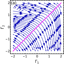
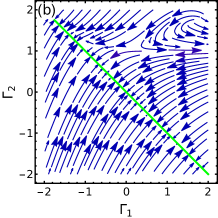
Figure 13: CRG at non-HS criticalities. (a) On the magenta line which capture the transition at $M_{1}$ ($\Gamma_{1}=\Gamma_{2}$). The transition line is characterized with the outward RG flow. (b) On the green line to capture the transition at $M_{2}$ ($\Gamma_{1}=-\Gamma_{2}$). The transition line is characterized with the inward RG flow.

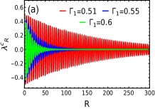
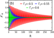
Figure 14: Wannier state correlation function at criticality. The parameter values $\Gamma_{0}=1$ and $\Gamma_{2}=0.5$ are fixed. (a) Represents $\lambda_{R}^{c}$ in the vicinity of $M_{1}$ i.e. $\Gamma_{1}=0.5$. (b) Represents $\lambda_{R}^{c}$ in the vicinity of $M_{2}$ i.e. $\Gamma_{1}=-0.5$.

V.2 Curvature function renormalization group and correlation function

We perform the scaling scheme at non-HS criticality and obtain RG equations of the model which essentially captures the topological transition between non-HS critical phases. From Eq.37, the RG equations for the magenta line can be obtained for the parameters $\Gamma_{1}$ and $\Gamma_{2}$ with $\Gamma_{0}=1$ as

$$\frac{d\Gamma_{1}}{dl}=\frac{(\Gamma_{1}+\alpha)^{4}\alpha\Lambda_{5}(\Gamma_{0},\Gamma_{1},\Gamma_{2})}{\Lambda_{6}(\Gamma_{0},\Gamma_{1},\Gamma_{2})}$$ (44)

$$\frac{d\Gamma_{2}}{dl}=-\frac{(\Gamma_{1}+\alpha)^{4}\alpha\alpha_{1}^{\prime}\Lambda_{5}(\Gamma_{0},\Gamma_{1},\Gamma_{2})}{\Lambda_{6}^{\prime}(\Gamma_{0},\Gamma_{1},\Gamma_{2})}$$ (45)

Similarly, for the green line we get

$$\frac{d\Gamma_{1}}{dl}=-\frac{(\Gamma_{1}-\alpha)^{4}\alpha\Lambda_{7}(\Gamma_{0},\Gamma_{1},\Gamma_{2})}{\Lambda_{8}(\Gamma_{0},\Gamma_{1},\Gamma_{2})}$$ (46)

$$\frac{d\Gamma_{2}}{dl}=-\frac{(\Gamma_{1}-\alpha)^{4}\alpha\alpha_{1}^{\prime}\Lambda_{7}(\Gamma_{0},\Gamma_{1},\Gamma_{2})}{\Lambda_{8}^{\prime}(\Gamma_{0},\Gamma_{1},\Gamma_{2})}$$ (47)

where $\alpha=\sqrt{\Gamma_{1}^{2}+4\Gamma_{0}(\Gamma_{0}-\Gamma_{2})}$ and $\alpha_{1}^{\prime}=(\Gamma_{2}-2\Gamma_{0})$ (see supplementary material for the detailed form of $\Lambda$s). The multicritical points $\Gamma_{1}=\pm\Gamma_{2}$ ($M_{1,2}$) are identified using the RG flow directions in $\Gamma_{1}-\Gamma_{2}$ plane. As shown in Fig.13, $M_{1}$ ($\Gamma_{1}=\Gamma_{2}$) manifest as a critical line with the flow lines flowing away. Similarly, $M_{2}$ ($\Gamma_{1}=-\Gamma_{2}$) manifest as a fixed line with flow lines flowing into, as explained in Eq.12. This clearly demonstrates that the multicritical points are indeed the topological phase transition points between non-HS critical phases at both the non-HS criticalities.

Apart from CRG, the correlation function defined at criticality in Eq.38 can be obtained to identify the topological transition between non-HS critical phases. The profile of the $\lambda_{R}^{c}$, for the non-HS $k_{0}^{mc}$, in the vicinity of multicritical points are shown in Fig.14. The correlation function decay slowly near $M_{1,2}$, i.e. $\Gamma_{1}=\pm 0.5$. The decay gets sharper as the parameters are tuned away the multicritical points. Therefore, this clearly shows that the multicritical points are the transition points between the non-HS critical phases.

VI Conclusions

In summary, we have identified a unique topological phase transition between non-HS critical phases through multicritical points. A generic model of topological insulators and superconductors have been constructed at criticality using the near-critical approach kumar2021topological , which provides an effective platform to study the edge mode solutions and topological transitions at non-HS criticalities.

The decay length of edge modes and winding number associated to the non-HS critical phases enables the characterization of trivial and topological non-HS critical phases both qualitatively and quantitatively. The decay length remains positive for non-trivial critical phases and negative for trivial critical phases. The multicritical point is associated with the divergence of the decay length, which indicate the delocalization of edge modes into the bulk. On the other hand, the winding number, which count the number of edge modes, acquires non-zero integer values at non-HS criticalities. This gives $w_{c}=2$ to a topological non-HS critical phase where only one edge mode is localized. Therefore, we have suggested to consider the difference in the winding numbers between trivial and non-trivial critical phases which yields the correct count of the edge modes localized at the non-trivial critical phase. The numerical solutions in the open boundary condition are found to be in agreement with these results.

We have also generalized the scaling theory to capture the topological transition at non-HS critical points. The scaling theory based on the divergence of curvature function, characterize both the conventional and the unique topological transition in terms of RG flow, critical exponents and correlation functions. Investigating the conventional topological transition between gapped phases, we have found that the CRG method is efficient to capture the non-HS critical points. Reframing the CRG method to work at criticality, we have identified the topological transition between non-HS critical phases through multicritical points. The critical and fixed line behaviors of the CRG equations in the parameter space is identified with RG flow rate and directions. In addition, the exponential decay of the correlation function near the multicritical points clearly evidence the unique topological transition between non-HS critical phases. Moreover, the divergence in curvature function along with the flipping of its sign across the transition points, locate the non-HS critical and multicritical points. The critical exponents of curvature function, calculated both analytically and numerically yields $\gamma=\nu=1$, which establish the universality class of non-HS critical points and multicritical points.

The model discussed in this work can be efficiently simulated using the superconducting circuit of a single qubit driven by the microwave pulses PhysRevB.101.035109 ; niu2021simulation and the ultracold atoms in optical lattices goldman2016topological ; xie2019topological ; an2018engineering ; meier2016observation ; kraus2012preparing ; jiang2011majorana ; an2018engineering . Therefore, using the good control over the nearest neighbors provided by these platforms one can study the results discussed in this work. As the non-HS criticality becomes prominent with increasing nearest-neighbor couplings hsu2020topological ; niu2012majorana ; kartik2021topological , an interesting question is whether the unique topological transition survive in truly long-range models. Moreover, the study of this interesting phenomena in non-Hermitian systems rahul2022topological , spin systems niu2012majorana and driven systems PhysRevLett.121.076802 ; molignini2018universal sets the future direction of the work. In addition, the fate of the edge modes and topological transition at non-HS criticality in the presence of interactions is an intriguing open problem. Therefore, we hope that our work will provide a step forward towards the understanding of the interesting interplay between topology and criticality. Moreover, the model considered in this study is not a true long-range model with decaying coupling strengths PhysRevLett.113.156402 ; PhysRevB.95.195160 . Nevertheless, the results discussed in this work will remain effective even with power-law decaying nearest-neighbor coupling strengths kartik2021topological . However, a detailed study, specifically, the topological transition between non-HS critical phases in truly long-range models remains a future scope of our work.

VII ACKNOWLEDGMENTS

RRK and SS would like to acknowledge DST (Department of Science and Technology, Government of India-CRG/2021/00996) for the the funding and support. YRK would like to thank AMEF (Admar Mutt Education Foundation) for the funding and support. Authors would like to thank Nilanjan Roy and Rahul S for the useful discussions.

References

- (1) F Duncan M Haldane. Phys. Rev. Lett. 61, 2015 (1988).
- (2) M Zahid Hasan and Charles L Kane. Rev. Mod. Phys. 82, 3045 (2010).
- (3) Jing Wang and Shou-Cheng Zhang. Nat. Mater. 16, 1062–1067 (2017).
- (4) Nathan Goldman, Jan C Budich, and Peter Zoller. Nat. Phys. 12, 639–645 (2016).
- (5) Prineha Narang, Christina AC Garcia, and Claudia Felser. Nat. Mater. 20, 293–300 (2021).
- (6) A Yu Kitaev. Phys. Usp. 44, 131 (2001).
- (7) Charles L Kane and Eugene J Mele. Phys. Rev. Lett. 95, 226801 (2005).
- (8) D. J. Thouless, M. Kohmoto, M. P. Nightingale, and M. den Nijs. Phys. Rev. Lett. 49, 405 (1982).
- (9) Michael V Berry. Proc. R. Soc. Lond. A. Mathematical and Physical Sciences, 392, 45–57 (1984).
- (10) J. Zak. Phys. Rev. Lett., 62, 2747–2750 (1989).
- (11) Alexander Altland and Martin R. Zirnbauer. Phys. Rev. B, 55, 1142–1161 (1997).
- (12) Sujit Sarkar. Sci. Rep., 8, 1–20 (2018).
- (13) Rahul S, Ranjith Kumar R, Y R Kartik, Amitava Banerjee, Sujit Sarkar. Phys. Scr., 94, 115803 (2019).
- (14) Y R Kartik, Ranjith R Kumar, S Rahul, Nilanjan Roy, and Sujit Sarkar. Phys. Rev. B. 104, 075113 (2021).
- (15) Wei Chen. J. Condens. Matter Phys. 28, 055601 (2016).
- (16) Wei Chen, Manfred Sigrist, and Andreas P Schnyder. J. Condens. Matter Phys. 28, 365501 (2016).
- (17) Wei Chen, Markus Legner, Andreas Rüegg, and Manfred Sigrist. Phys. Rev. B. 95, 075116 (2017).
- (18) Wei Chen. Phys. Rev. B. 97, 115130 (2018).
- (19) Wei Chen and Andreas P Schnyder. New J. Phys. 21, 073003 (2019).
- (20) Paolo Molignini, Wei Chen, and Ramasubramanian Chitra. Phys. Rev. B. 98, 125129 (2018).
- (21) S Panahiyan, W Chen, and S Fritzsche. Phys. Rev. B, 102, 134111 (2020).
- (22) Paolo Molignini, Wei Chen, and R Chitra. Phys. Rev. B. 101, 165106 (2020).
- (23) Faruk Abdulla, Priyanka Mohan, and Sumathi Rao. Phys. Rev. B. 102, 235129 (2020).
- (24) M Malard, H Johannesson, and W Chen. Phys. Rev. B. 102, 205420 (2020).
- (25) Paolo Molignini, R Chitra, and Wei Chen. Europhys. Lett. 128, 36001 (2020).
- (26) Ranjith R Kumar, Y R Kartik, S Rahul, and Sujit Sarkar. Sci. Rep. 11, 1–20 (2021).
- (27) Mucio A Continentino, Sabrina Rufo, and Griffith M Rufo. Finite size effects in topological quantum phase transitions. Strongly Coupled Field Theories for Condensed Matter and Quantum Information Theory, Springer Proceedings in Physics 239 (2020).
- (28) Ruben Verresen, Nick G Jones, and Frank Pollmann. Phys. Rev. Lett. 120, 057001 (2018).
- (29) Ruben Verresen, Ryan Thorngren, Nick G Jones, and Frank Pollmann. Phys. Rev. X. 11, 041059 (2021).
- (30) Nick G Jones and Ruben Verresen. J. Stat. Phys. 175, 1164–1213 (2019).
- (31) Ruben Verresen. arXiv:2003.05453v1 [cond-mat.str-el] (2020).
- (32) S Rahul, Ranjith R Kumar, Y R Kartik, and Sujit Sarkar. J. Phys. Soc. Jpn. 90, 094706 (2021).
- (33) Sen Niu, Yucheng Wang, and Xiong-Jun Liu. arXiv:2106.13400v2 [cond-mat.str-el] (2021).
- (34) Ryan Thorngren, Ashvin Vishwanath, and Ruben Verresen. Phys. Rev. B. 104, 075132 (2021).
- (35) Oleksandr Balabanov, Daniel Erkensten, and Henrik Johannesson. Phys. Rev. Res. 3, 043048 (2021).
- (36) Joana Fraxanet, Daniel González-Cuadra, Tilman Pfau, Maciej Lewenstein, Tim Langen, and Luca Barbiero. Phys. Rev. Lett. 128, 043402 (2022).
- (37) Anna Keselman, Erez Berg. Phys. Rev. B. 91, 235309 (2015).
- (38) Thomas Scaffidi, Daniel E. Parker, Romain Vasseur. Phys. Rev. X. 7, 041048 (2017).
- (39) Carlos M. Duque, Hong-Ye Hu, Yi-Zhuang You, Vedika Khemani, Ruben Verresen, and Romain Vasseur. Phys. Rev. B. 103, L100207 (2021).
- (40) Ranjith R Kumar, Nilanjan Roy, Y R Kartik, S Rahul, and Sujit Sarkar. arXiv:2112.02485v2 [cond-mat.str-el], (2021).
- (41) Rufo, S., Lopes, N., Continentino, M.A. and Griffith, M.A.R. Phys. Rev. B. 100, 195432 (2019).
- (42) Mariana Malard, David Brandao, Paulo Eduardo de Brito, and Henrik Johannesson. Phys. Rev. Res., 2, 033246 (2020).
- (43) Karin Sim, R Chitra, and Paolo Molignini. arXiv:2207.10676v2 [cond-mat.stat-mech], (2022).
- (44) Hsiu-Chuan Hsu and Tsung-Wei Chen. Phys. Rev. B. 102, 205425 (2020).
- (45) Yuezhen Niu, Suk Bum Chung, Chen-Hsuan Hsu, Ipsita Mandal, S Raghu, and Sudip Chakravarty. Phys. Rev. B. 85, 035110 (2012).
- (46) W. P. Su, J. R. Schrieffer, and A. J. Heeger. Phys. Rev. Lett. 42, 1698–1701 (1979).
- (47) Shuichi Murakami. Physica E: Low-dimensional Systems and Nanostructures. 43, 748–754 (2011).
- (48) Stefanos Kourtis, Titus Neupert, Christopher Mudry, Manfred Sigrist, and Wei Chen. Phys. Rev. B. 96, 205117 (2017).
- (49) Somenath Jalal, Rishabh Khare, and Siddhartha Lal. Topological transitions in ising models (2016).
- (50) Shun-Qing Shen, Wen-Yu Shan, and Hai-Zhou Lu. Topological insulator and the dirac equation. In Spin, 1, 33–44, World Scientific (2011).
- (51) Jie Lu, Wen-Yu Shan, Hai-Zhou Lu, and Shun-Qing Shen. New J. Phys., 13, 103016 (2011).
- (52) Roman Jackiw and Cláudio Rebbi. Phys. Rev. D, 13, 3398 (1976).
- (53) Ziyu Tao, Tongxing Yan, Weiyang Liu, Jingjing Niu, Yuxuan Zhou, Libo Zhang, Hao Jia, Weiqiang Chen, Song Liu, Yuanzhen Chen, and Dapeng Yu. Phys. Rev. B. 101, 035109, (2020).
- (54) Jingjing Niu, Tongxing Yan, Yuxuan Zhou, Ziyu Tao, Xiaole Li, Weiyang Liu, Libo Zhang, Hao Jia, Song Liu, Zhongbo Yan, et al. Sci. Bull. 66, 1168–1175 (2021).
- (55) Dizhou Xie, Wei Gou, Teng Xiao, Bryce Gadway, and Bo Yan. npj Quantum Inf. 5, 1–5 (2019).
- (56) Fangzhao Alex An, Eric J Meier, and Bryce Gadway. Phys. Rev. X. 8, 031045 (2018).
- (57) Eric J Meier, Fangzhao Alex An, and Bryce Gadway. Nat. Commun. 7, 1–6 (2016).
- (58) Christina V Kraus, Sebastian Diehl, Peter Zoller, and Mikhail A Baranov. New J. Phys. 14, 113036 (2012).
- (59) Liang Jiang, Takuya Kitagawa, Jason Alicea, AR Akhmerov, David Pekker, Gil Refael, J Ignacio Cirac, Eugene Demler, Mikhail D Lukin, and Peter Zoller. Phys. Rev. Lett. 106, 220402 (2011).
- (60) S Rahul and Sujit Sarkar. Sci. Rep., 12, 1–12 (2022).
- (61) Daniel Yates, Yonah Lemonik, Aditi Mitra. Phys. Rev. Lett. 121, 076802 (2018).
- (62) Davide Vodola, Luca Lepori, Elisa Ercolessi, Alexey V. Gorshkov, and Guido Pupillo. Phys. Rev. Lett. 113, 156402 (2014).
- (63) Antonio Alecce and Luca Dell’Anna. Phys. Rev. B. 95, 195160 (2017).