Efficient Multi-order Gated Aggregation Network

Abstract

Since the recent success of Vision Transformers (ViTs), explorations toward ViT-style architectures have triggered the resurgence of ConvNets. In this work, we explore the representation ability of modern ConvNets from a novel view of multi-order game-theoretic interaction, which reflects inter-variable interaction effects w.r.t. contexts of different scales based on game theory. Within the modern ConvNet framework, we tailor the two feature mixers with conceptually simple yet effective depthwise convolutions to facilitate middle-order information across spatial and channel spaces respectively. In this light, a new family of pure ConvNet architecture, dubbed MogaNet, is proposed, which shows excellent scalability and attains competitive results among state-of-the-art models with more efficient use of parameters on ImageNet and multifarious typical vision benchmarks, including COCO object detection, ADE20K semantic segmentation, 2D&3D human pose estimation, and video prediction. Typically, MogaNet hits 80.0% and 87.8% top-1 accuracy with 5.2M and 181M parameters on ImageNet, outperforming ParC-Net-S and ConvNeXt-L while saving 59% FLOPs and 17M parameters. The source code is available at https://github.com/Westlake-AI/MogaNet.

1 Introduction

Convolutional Neural Networks (ConvNets) have been the method of choice for computer vision [53, 106, 69] since the renaissance of deep neural networks (DNNs) [70]. By interleaving hierarchical convolutional layers in-between pooling and non-linear operations [71, 149, 112, 113], ConvNets can encode underlying semantic patterns of observed images with the built-in translation equivariance constraints [53, 159, 91, 148, 60, 163] and have further become the fundamental infrastructure in today’s computer vision systems. Nevertheless, representations learned by ConvNets have been proven to have a strong bias on local texture [128], resulting in a serious detriment of global information [6, 56, 36]. Therefore, efforts have been made to upgrade macro-level architectures [21, 148, 103, 163] and context aggregation modules [29, 137, 60, 139, 13].

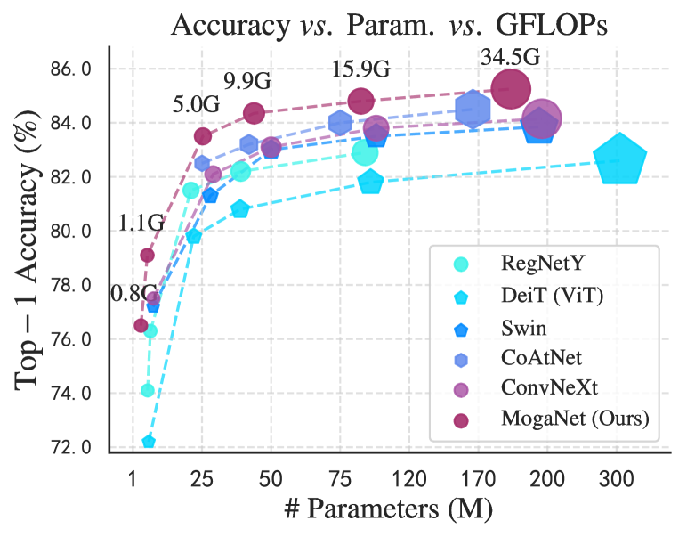
Figure 1: Performance on ImageNet-1K validation set at $224^{2}$ resolutions. MogaNet with pure Convolutions outperforms Transformers (DeiT[122] and Swin [85]), ConvNets (RegNetY [103] and ConvNeXt [86]), and hybrid models (CoAtNet [30]) at all parameter scales.

In contrast, by relaxing local inductive bias, the newly emerged Vision Transformers (ViTs) [38, 85, 135, 23] have rapidly challenged the long dominance of ConvNets on a wide range of vision benchmarks. There is an almost unanimous consensus that such superiority of ViTs primarily stems from self-attention mechanism [5, 129], which facilitates long-term feature interactions regardless of the topological distance. From a practical standpoint, however, quadratic complexity within self-attention modelling prohibitively restricts the computational efficiency of ViTs [134, 61, 140] and its application potential to fine-grained scenarios [87, 65, 168] where high-resolution features are required. In addition, the absence of inductive bias shatters the inherent geometric structure of images, thereby inevitably inducing the detriment of neighborhood correlations [100]. To tackle this obstacle, endeavors have been contributed to reintroduce pyramid-like hierarchical layouts [85, 40, 135] and shift-invariant priors [141, 30, 49, 72, 19] to ViTs, at the expense of model generality and expressiveness.

More recent studies have shown that the representation capability of ViTs should mainly be credited to their macro-level architectures rather than the commonly-conjectured self-attention mechanisims [121, 104, 154]. More importantly, with advanced training setup and ViT-style architecture modernization, ConvNets can readily deliver excellent scalability and competitive performance w.r.t. well-tuned ViTs across a variety of visual benchmarks [138, 86, 36, 100], which heats the debate between ConvNets and ViTs and further alters the roadmap for deep architecture design.

Different from previous attempts, we investigate the representation capacity of modern ConvNets through the lens of multi-order game-theoretic interaction [1], which provides a new view to explain the feature interaction behaviors and effects encoded in a deep architecture based on game theory. As shown in Fig. 3b, most modern DNNs are inclined to encode game-theoretic interaction of extremely low or high complexities rather than the most discriminative intermediate one [33], which limits their representation abilities and robustness to complex samples.

Under this perspective, we develop a novel pure ConvNet architecture called Multi-order gated aggregation Network (MogaNet) for balancing the multi-order interaction strength, in order to improve the performance of ConvNets. Our design encapsulates both low-order locality priors and middle-order context aggregation into a unified spatial aggregation block, where features of balanced multi-order interactions are efficiently congregated and contextualized with the gating mechanism in parallel. From the channel aspect, as existing methods are prone to channel information redundancy [104, 61], we tailor a conceptually simple yet efficient channel aggregation block, which performs adaptive channel-wise feature reallocation to the multi-order input and significantly outperforms prevailing counterparts (e.g., SE module [60]) with lower computational cost.

Extensive experiments demonstrate the impressive performance and great efficiency of MogaNet at different model scales on various computer vision tasks, including image classification, object detection, semantic segmentation, instance segmentation, pose estimation, etc. As a result, MogaNet attains 83.4% and 87.8% with 25M and 181M parameters, which exhibits favorable computational overhead compared with existing small-size models, as shown in Fig. 1. MogaNet-T achieves 80.0% top-1 accuracy on ImageNet-1K, outperforming the state-of-the-art ParC-Net-S [161] by 1.0% with 2.04G lower FLOPs under the same setting. Moreover, MogaNet exhibits strong performance gains on various downstream tasks, e.g., surpassing Swin-L [85] by 2.3% AP^b on COCO detection with fewer parameters and computational budget. Therefore, the performance gains of MogaNet are not due to increased capacity but rather to more efficient use of model parameters.

2 Related Work

2.1 Vision Transformers

Since the significant success of Transformer [129] in natural language processing (NLP) [35, 10], Vision Transformer (ViT) [38] is proposed and has attained promising results on ImageNet [34]. However, compared with ConvNets, pure ViTs are more over-parameterized and rely on large-scale pre-training [38, 7, 51, 75]. Targeting this problem, one branch of researchers proposes lightweight ViTs [147, 93, 77, 18] with efficient attention variants [134]. Meanwhile, the incorporation of self-attention and convolution as a hybrid backbone has been vigorously studied [47, 141, 30, 31, 72, 96, 111] for imparting regional priors to ViTs. By introducing inductive bias [14, 168, 16, 98, 65, 3], advanced training strategies [122, 123, 155, 125] or extra knowledge [66, 78, 143], ViT and its variants can achieve competitive performance as ConvNets and have been extended to various computer vision areas.

MetaFormer [154] as shown in Fig. 2 substantially influenced the principle of deep architecture design, where all ViTs [122, 127, 130] can be classified by how they treat the token-mixing approaches, such as relative position encoding [142], local window shifting [85] and MLP layer [121], etc. It primarily comprises three cardinal components: (i) embedding stem, (ii) spatial mixing block, and (iii) channel mixing block. The embedding stem downsamples the input image to reduce image-inherent redundancies and computational overload. We assume the input feature $X$ and the output $Z$ are in the same shape $\mathbb{R}^{C\times H\times W}$, we have:

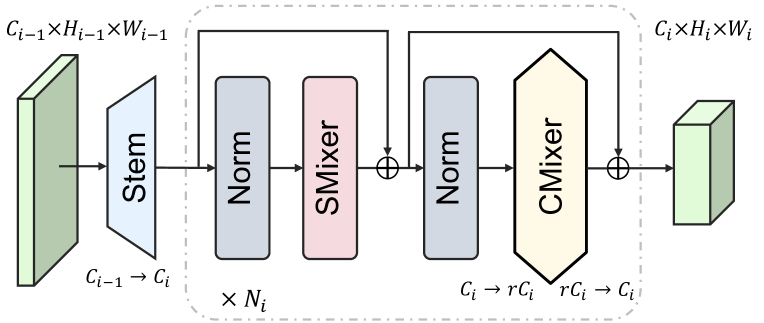
Figure 2: Illustration of the macro architecture. It has 4 stages in hierarchical, and $i$-th stage contains an embedding stem and $N_{i}$ blocks of $\mathrm{SMixer}(\cdot)$ and $\mathrm{CMixer}(\cdot)$ with PreNorm [133] and identical connection [53]. The features within the $i$-th stage are in the same shape, except that $\mathrm{CMixer}(\cdot)$ will increase the dimension to $rC_{i}$ with an expand ratio $r$ as an inverted bottleneck [107].

$$Z=\mathrm{Stem}(X),\vspace{-0.40em}$$ (1)

where $Z$ is downsampled features, e.g.,. Then, the feature flows to a stack of residual blocks. In each stage, the network modules can be decoupled into two separate functional components, $\mathrm{SMixer}(\cdot)$ and $\mathrm{CMixer}(\cdot)$ for spatial-wise and channel-wise information propagation [154],

$$Y=X+\mathrm{SMixer}\big{(}\mathrm{Norm}(X)\big{)},\vspace{-0.50em}$$ (2)

$$Z=Y+\mathrm{CMixer}\big{(}\mathrm{Norm}(Y)\big{)},\vspace{-0.20em}$$ (3)

where $\mathrm{Norm}(\cdot)$ is a normalization layer, e.g., Batch Normalization [63] (BN). Notice that $\mathrm{SMixer}(\cdot)$ could be various spatial operations (e.g., self-attention [129], convolution), while $\mathrm{CMixer}(\cdot)$ is usually achieved by channel-wise MLP in inverted bottleneck [107] and an expand ratio of $r$.

2.2 Post-ViT Modern ConvNets

By taking the merits of ViT-style macro-level architecture [154], modern ConvNets [127, 86, 36, 82, 105, 150] show thrilling performance with large depth-wise convolutions [50] for global context aggregation. Similar to ViTs, context aggregation operations in modern ConvNets can be summerized as a group of components that adaptively emphasize contextual information and decrease trivial redundancies in spatial mixing between two embedded features:

$$O=\mathcal{S}\big{(}\mathcal{F}_{\phi}(X),\mathcal{G}_{\psi}(X)\big{)},\vspace{-0.40em}$$ (4)

where $\mathcal{F}_{\phi}(\cdot)$ and $\mathcal{G}_{\psi}(\cdot)$ are the aggregation and context branches with parameters $\phi$ and $\psi$. Context aggregation models the importance of each position on $X$ by the aggregation branch $\mathcal{F}_{\phi}(X)$ and reweights the embedded feature from the context branch $\mathcal{G}_{\psi}(X)$ by $\mathcal{S}(\cdot,\cdot)$.

Method	$\mathcal{S}(\cdot,\cdot)$	$\mathcal{F}_{\phi}(\cdot)$	$\mathcal{G}_{\psi}(\cdot)$
Self-attention [129]	$<\cdot,\cdot>$	$\mathrm{Softmax}\big{(}C^{\frac{1}{2}}XW_{Q}(XW_{K})^{T}\big{)}$	$XW_{V}$
Linear attention [134]	$<\cdot,\cdot>$	$\mathrm{Softmax}\big{(}C^{\frac{1}{2}}XW_{Q}(W_{E}XW_{K})^{T}\big{)}$	$W_{F}XW_{V}$
GLU [32]	$\odot$	$\mathrm{Sigmoid}(XW_{\phi})$	$XW_{\psi}$
SE [60]	$\odot$	$\mathrm{Sigmoid}\big{(}\big{(}\mathrm{GAP}(X)W_{\phi}\big{)}W_{\psi}\big{)}$	$X$

Table 1: Examples of context aggregation methods according to Eq. (4). The sing-head version of self-attention and linear attention is presented as an illustration and $W$ denotes a linear projection.

As shown in Table 1, there are mainly two types of context aggregations for modern ConvNets: self-attention mechanism [129, 137, 38] and gating attention [32, 60]. The importance of each position on $X$ is calculated by global interactions of all other positions in $\mathcal{F}_{\phi}(\cdot)$ with a dot-product, which results in quadratic computational complexity. To overcome this limitation, attention variants in linear complexity [90, 102] were proposed to substitute vanilla self-attention, e.g., linear attention [134, 95] in the second line of Table 1, but they might degenerate to trivial attentions [140]. Unlike self-attention, gating unit employs an element-wise product $\odot$ as $\mathcal{S}(\cdot,\cdot)$ in linear complexity, e.g., gated linear unit (GLU) variants [109] and squeeze-and-excitation (SE) modules [60] in the last two lines of Table 1.

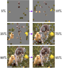
(a)

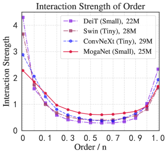
(b)

Figure 3: (a) Illustrations of representation bottleneck. Humans can recognize the object from images with around 50% patches while learning little new information with a few (e.g., 5$\sim$10%) or finding it too redundant with almost all patches (e.g., 90$\sim$95%). DNNs are inclined to extract the most information from very few or the most patches but usually have less information gain with 20$\sim$80% patches. (b) Distributions of the interaction strength $J^{(m)}$ are plotted for Transformers and ConvNets on ImageNet-1K with $224^{2}$ resolutions and $n$ = $14\times 14$. Middle-order interactions mean the middle-complex interaction, where a medium number of patches (e.g., 0.2$\sim$0.8n) participate.

3 Representation Bottleneck from the View of Multi-order Game-theoretic Interaction

Recent analysis towards the robustness [94, 166, 97] and generalization ability [44, 2, 128, 43] of DNNs delivers a new perspective to improve deep architectures. Apart from these efforts, we extend the scope to the investigation of multi-order game-theoretic interaction. As shown in Fig. 3a, DNNs can still recognize the target object under extreme occlusion ratios (e.g., only 10$\sim$20% visible patches) but produce less information gain with intermediate occlusions [33, 94]. Interestingly, our human brains attain the sharpest knowledge upsurge from images with around 50% patches, which indicates an intriguing cognition gap between human vision and deep models. Formally, it can be explained by $m$-th order game-theoretic interaction $I^{(m)}(i,j)$ and $m$-order interaction strength $J^{(m)}$, as defined in [162, 33]. Considering the image with $n$ patches in total, $I^{(m)}(i,j)$ measures the average interaction complexity between the patch pair $i,j$ over all contexts consisting of $m$ patches, where $0\leq m\leq n-2$ and the order $m$ reflects the scale of the context involved in the game-theoretic interactions between pixels $i$ and $j$. Normalized by the average of interaction strength, the relative interaction strength $J^{(m)}$ with $m\in(0,1)$ measures the complexity of interactions encoded in DNNs. Notably, low-order interactions tend to encode common or widely-shared local texture and the high-order ones are inclined to forcibly memorize the pattern of rare outliers [33, 20]. Refer to Appendix B.1 for definitions and details. As shown in Fig. 3b, most DNNs are more favored to encode excessively low-order or high-order game-theoretic interactions while typically suppressing the most flexible and discriminative middle-order ones [33, 20]. From our perspective, such dilemma in both ConvNets and ViTs may be attributed to the inappropriate composition of convolutional inductive bias and context aggregations [126, 128, 33, 75]. In particular, a naive implementation of self-attention or convolutions can be intrinsically prone to the strong bias of global shape [43, 36] or local texture [56], infusing spurious extreme-order game-theoretic interaction preference into deep networks.

4 Methodology

4.1 Overview of MogaNet

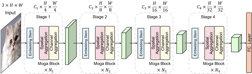
Figure A1: The overall architecture of MogaNet. Similar to [53, 85, 154, 86], MogaNet uses hierarchical architectures of 4 stages. The stage $i$ consists of an embedding stem and $N_{i}$ Moga Blocks, which contain spatial aggregation blocks and channel aggregation blocks.

Based on Fig. 2, we design the four-stage MogaNet architecture, illustrated in Fig. A1. For stage $i$, the input image or feature is first fed into the embedding stem to regulate the feature resolutions and embed into $C_{i}$ dimensions. Assuming the input image in $H\times W$ resolutions, features of the four stages are in $\frac{H}{4}\times\frac{W}{4}$, $\frac{H}{8}\times\frac{W}{8}$, $\frac{H}{16}\times\frac{W}{16}$, and $\frac{H}{32}\times\frac{W}{32}$ resolution respectively. Then, the embedded feature flows into $N_{i}$ Moga Blocks, consisting of spatial and channel aggregation blocks as presented in Sec. 4.2 and 4.3, for further context extraction and aggregation. After the final output, GAP and a linear layer are added for classification tasks. As for dense prediction tasks [52, 146], the output from four stages can be used through neck modules [79, 69].

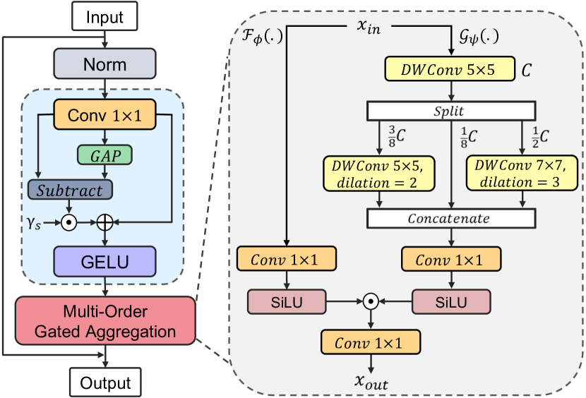
Figure 4: Structure of spatial aggregation block $\mathrm{Moga}(\cdot)$.

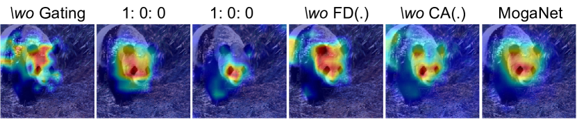
Figure 5: Grad-CAM visualization of ablations. 1: 0: 0 and 0: 0: 1 denote only using $C_{l}$ or $C_{h}$ for Multi-order DWConv Layers. Models with extremely low- ($C_{l}$) or high- ($C_{h}$) order interactions are sensitive to similar regional textures (1: 0: 0) or excessive discriminative parts (0: 0: 1), not localizing semantic parts. Gating can effectively eliminate the disturbing contextual noise ($\backslash$wo Gating).

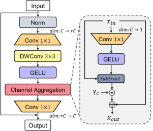
(a)

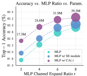
(b)

Figure 6: (a) Structure of channel aggregation block. (b) Analysis of channel MLP and the channel aggregation module. Based on MogaNet-S, performances and model sizes of the raw channel MLP, MLP with SE block, and the channel aggregation is compared with the MLP ratio of $\{2,4,6,8\}$ on ImageNet-1K.

Modules		Top-1	Params.	FLOPs
		Acc (%)	(M)	(G)
Baseline		76.6	4.75	1.01
SMixer	+Gating branch	77.3	5.09	1.07
	+$\mathrm{DW}_{7\times 7}$	77.5	5.14	1.09
	+Multi-order $\mathrm{DW}(\cdot)$	78.0	5.17	1.10
	+$\mathrm{FD(\cdot)}$	78.3	5.18	1.10
CMixer	+SE module	78.6	5.29	1.14
	+$\mathrm{CA}(\cdot)$	79.0	5.20	1.10

Table 2: Ablation of designed modules on ImageNet-1K. The baseline uses the non-linear projection and $\mathrm{DW}_{5\times 5}$ as $\mathrm{SMixer}(\cdot)$ and the vanilla MLP as $\mathrm{CMixer}(\cdot)$. Gray denotes the designed modules. Compared to $\mathrm{DW}_{7\times 7}$ and SE modules, Multi-order $\mathrm{DW}(\cdot)$+$\mathrm{FD(\cdot)}$ as multi-order regionality perceptions and $\mathrm{CA}(\cdot)$ bring significant improvements with a little extra cost.

4.2 Multi-order Gated Aggregation

As discussed in Sec. 3, conventional DNNs with the incompatible composition of locality perception and context aggregation are inclined to concentrate on extreme-order interactions while suppressing the most discriminative middle-order ones [72, 100, 33]. As shown in Fig. 5, the primary challenge is how to capture contextual representation with balanced multi-order game-theoretic interactions efficiently. To this end, we propose a spatial aggregation (SA) block as $\mathrm{SMixer}(\cdot)$ to aggregate multi-order contexts in a unified design, as shown in Fig. 4, consisting of two cascaded components. We rewrite Eq. (2) as:

$$Z=X+\mathrm{Moga}\Big{(}\mathrm{FD}\big{(}\mathrm{Norm}(X)\big{)}\Big{)},\vspace{-0.40em}$$ (5)

where $\mathrm{FD}(\cdot)$ indicates a feature decomposition module (FD) and $\mathrm{Moga}(\cdot)$ is a multi-order gated aggregation module comprising the gating $\mathcal{F}_{\phi}(\cdot)$ and context branch $\mathcal{G}_{\psi}(\cdot)$.

Multi-order contexts.

As a pure convolutional structure, we extract multi-order features with both static and adaptive locality perceptions. Except for $m$-order interactions, there are two complementary counterparts, $0$-order interaction of common local texture and ‘$n$-order’ interaction covering complex global shape, which are modelled by $\mathrm{Conv}_{1\times 1}(\cdot)$ and $\mathrm{GAP}(\cdot)$ respectively. To force the network focus on balancing interactions of multiple complexities, we propose $\mathrm{FD}(\cdot)$ to dynamically exclude trivial feature interactions, defined as:

$$Y =\mathrm{Conv}_{1\times 1}(X),$$ (6)

$$Z =\mathrm{GELU}\Big{(}Y+\gamma_{s}\odot\big{(}Y-\mathrm{GAP}(Y)\big{)}\Big{)},\vspace{-0.6em}$$ (7)

where ${\gamma}_{s}\in\mathbb{R}^{C\times 1}$ denotes a scaling factor initialized as zeros. By re-weighting the complimentary interaction component $Y-\mathrm{GAP}(Y)$, $\mathrm{FD}(\cdot)$ also increases spatial feature diversities [97, 132]. Then, we ensemble depth-wise convolutions (DWConv) to encode multi-order features in the context branch of $\mathrm{Moga}(\cdot)$. Unlike previous works that simply combine DWConv with self-attentions to model local and global interactions [161, 95, 111, 105] , we employ three different DWConv layers with dilation ratios $d\in\{1,2,3\}$ in parallel to capture low, middle, and high-order interactions: given the input feature $X\in\mathbb{R}^{C\times HW}$, $\mathrm{DW}_{5\times 5,d=1}$ is first applied for low-order features; then, the output is factorized into ${X}_{l}\in\mathbb{R}^{C_{l}\times HW}$, ${X}_{m}\in\mathbb{R}^{C_{m}\times HW}$, and ${X}_{h}\in\mathbb{R}^{C_{h}\times HW}$ along the channel dimension, where $C_{l}+C_{m}+C_{h}=C$; afterward, ${X}_{m}$ and ${X}_{h}$ are assigned to $\mathrm{DW}_{5\times 5,d=2}$ and $\mathrm{DW}_{7\times 7,d=3}$, respectively, while ${X}_{l}$ serves as identical mapping; finally, the output of ${X}_{l}$, ${X}_{m}$, and ${X}_{h}$ are concatenated to form multi-order contexts, $Y_{C}=\mathrm{Concat}(Y_{l,1:C_{l}},Y_{m},Y_{h})$. Notice that the proposed $\mathrm{FD}(\cdot)$ and multi-order DWConv layers only require a little extra computational overhead and parameters in comparison to $\mathrm{DW}_{7\times 7}$ used in ConvNeXt [86], e.g., +multi-order and +$\mathrm{FD}(\cdot)$ increase 0.04M parameters and 0.01G FLOPS over $\mathrm{DW}_{7\times 7}$ as shown in Table 2.

Gating aggregation.

To aggregate the multi-order features from the context branch, we employ SiLU [39] activation in the gating branch, i.e., $x\cdot\mathrm{Sigmoid}(x)$, which can be regarded an advanced version of Sigmoid. As verified in Appendix C.1, we find that SiLU owns both the gating effects as Sigmoid and the stable training property. Taking the output from $\mathrm{FD}(\cdot)$ as the input, we rewrite Eq. (4) as:

$$Z =\underbrace{\mathrm{SiLU}\big{(}\mathrm{Conv}_{1\times 1}(X)\big{)}}_{\mathcal{F}_{\phi}}\odot\underbrace{\mathrm{SiLU}\big{(}\mathrm{Conv}_{1\times 1}(Y_{C})\big{)}}_{\mathcal{G}_{\psi}},\vspace{-1.5em}$$ (8)

With the proposed SA blocks, MogaNet captures more middle-order interactions, as validated in Fig. 3b. The SA block produces discriminative multi-order representations with similar parameters and FLOPs as $\mathrm{DW}_{7\times 7}$ in ConvNeXt, which is well beyond the reach of existing methods without the cost-consuming self-attentions.

4.3 Multi-order Feature Reallocation by Channel Aggregation

Prevailing architectures, as illustrated in Sec. 2, perform channel-mixing $\mathrm{CMixer}(\cdot)$ mainly by two linear projections, e.g., 2-layer channel MLP [38, 85, 121] with a channel expand ratio $r$ or the MLP with a $3\times 3$ DWConv in between [136, 96, 95]. Due to the inherent redundancy cross channels [139, 13, 119, 131], vanilla MLP requires a number of parameters ($r$ default to 4 or 8) to achieve expected performance, showing low computational efficiency as plotted in Fig. 6b. To address this issue, most current methods directly insert a channel enhancement module, e.g., SE module [60], into MLP. Unlike these designs requiring additional MLP bottleneck, we introduce a lightweight channel aggregation module $\mathrm{CA}(\cdot)$ to conduct adaptive channel-wise reallocation in high-dimensional hidden spaces and further extend it to a channel aggregation (CA) block. As shown in Fig. 6a, we rewrite Eq. (3) for our CA block as:

$$Y =\mathrm{GELU}\Big{(}\mathrm{DW_{3\times 3}}\big{(}\mathrm{Conv_{1\times 1}}(\mathrm{Norm}(X))\big{)}\Big{)},$$ (9)

$$Z =\mathrm{Conv_{1\times 1}}\big{(}\mathrm{CA}(Y)\big{)}+X.$$

Concretely, $\mathrm{CA}(\cdot)$ is implemented by a channel-reducing projection $W_{r}:\mathbb{R}^{C\times HW}\rightarrow\mathbb{R}^{1\times HW}$ and GELU to gather and reallocate channel-wise information:

$$\mathrm{CA}(X)=X+\gamma_{c}\odot\big{(}X-\mathrm{GELU}(XW_{r})\big{)},\vspace{-0.4em}$$ (10)

where $\gamma_{c}$ is the channel-wise scaling factor initialized as zeros, which reallocates the complementary channel-wise interactions $X-\mathrm{GELU}(XW_{r})$. As shown in Fig. 7, $\mathrm{CA}(\cdot)$ effectively boosts middle-order game-theoretic interactions. Fig. 6b verifies the superiority of $\mathrm{CA}(\cdot)$ compared with the vanilla MLP and the MLP with SE module in eliminating channel-wise information redundancy. Despite some improvements to the baseline, the MLP $w/$ SE module still requires large MLP ratios (e.g., $r$ = 6) to achieve expected performance while introducing extra parameters and computational overhead. In contrast, our $\mathrm{CA}(\cdot)$ with $r$ = 4 brings 0.6% gain over the baseline at a small extra cost (0.04M extra parameters and 0.01G FLOPs) while achieving the same performance as the baseline with $r$ = 8.

4.4 Implementation Details

Following the network design style of ConvNets [86], we scale up MogaNet for six model sizes (X-Tiny, Tiny, Small, Base, Large, and X-Large) via stacking the different number of spatial and channel aggregation blocks at each stage, which has similar numbers of parameters as RegNet [103] variants. Network configurations and hyper-parameters are detailed in Table A1. FLOPs and throughputs are analyzed in Appendix C.3. We set the channels of the multi-order DWConv layers to $C_{l}:$ $C_{m}:$ $C_{h}$ = 1:3:4 (see Appendix C.2). Similar to [124, 72, 77], the first embedding stem in MogaNet is designed as two stacked 3$\times$3 convolution layers with the stride of 2 while adopting the single-layer version for embedding stems in other three stages. We select GELU [54] as the common activation function and only use SiLU in the Moga module as Eq. (8).

5 Experiments

To verify and compare MogaNet with the leading network architectures, we conduct extensive experiments on popular vision tasks, including image classification, object detection, instance and semantic segmentation, 2D and 3D pose estimation, and video prediction. Experiments are implemented with PyTorch and run on NVIDIA A100 GPUs.

5.1 ImageNet Classification

Settings.

For classification experiments on ImageNet [34], we train MogaNet variants following the standard procedure [122, 85] on ImageNet-1K (IN-1K) for a fair comparison, training 300 epochs with AdamW [89] optimizer, a basic learning rate of $1\times 10^{-3}$, and a Cosine scheduler [88]. To explore the capacities of large models, we pre-trained MogaNet-XL on ImageNet-21K (IN-21K) for 90 epochs and then fine-tuned 30 epochs on IN-1K following [86]. Appendix A.2 and D.1 provide implementation details and more results. We compare three typical architectures: Pure ConvNets (C), Transformers (T), and Hybrid model (H) with both self-attention and convolution operations.

Architecture	Date	Type	Image	Param.	FLOPs	Top-1
			Size	(M)	(G)	Acc (%)
ResNet-18† [53]	CVPR’2016	C	$224^{2}$	11.7	1.80	71.5
ShuffleNetV2 $2\times$ [92]	ECCV’2018	C	$224^{2}$	5.5	0.60	75.4
EfficientNet-B0 [119]	ICML’2019	C	$224^{2}$	5.3	0.39	77.1
MobileNetV3 $1\times$ [59]	ICCV’2019	C	$224^{2}$	5.4	0.23	75.2
RegNetY-800MF [103]	CVPR’2020	C	$224^{2}$	6.3	0.80	76.3
DeiT-T† [122]	ICML’2021	T	$224^{2}$	5.7	1.08	74.1
PVT-T [135]	ICCV’2021	T	$224^{2}$	13.2	1.60	75.1
T2T-ViT-7 [156]	ICCV’2021	T	$224^{2}$	4.3	1.20	71.7
ViT-C [147]	NIPS’2021	T	$224^{2}$	4.6	1.10	75.3
SReT-TDistill [110]	ECCV’2022	T	$224^{2}$	4.8	1.10	77.6
PiT-Ti [55]	ICCV’2021	H	$224^{2}$	4.9	0.70	74.6
LeViT-S [45]	ICCV’2021	H	$224^{2}$	7.8	0.31	76.6
CoaT-Lite-T [76]	ICCV’2021	H	$224^{2}$	5.7	1.60	77.5
Swin-1G [85]	ICCV’2021	H	$224^{2}$	7.3	1.00	77.3
MobileViT-S [93]	ICLR’2022	H	$256^{2}$	5.6	4.02	78.4
MobileFormer-294M [19]	CVPR’2022	H	$224^{2}$	11.4	0.59	77.9
ConvNext-XT [86]	CVPR’2022	C	$224^{2}$	7.4	0.60	77.5
VAN-B0 [48]	arXiv’2022	C	$224^{2}$	4.1	0.88	75.4
ParC-Net-S [161]	ECCV’2022	C	$256^{2}$	5.0	3.48	78.6
MogaNet-XT	Ours	C	$256^{2}$	3.0	1.04	77.2
MogaNet-T	Ours	C	$224^{2}$	5.2	1.10	79.0
MogaNet-T§	Ours	C	$256^{2}$	5.2	1.44	80.0

Table 3: Image classification of lightweight ($\sim$5M parameters) models on IN-1K validation set. ${\dagger}$ and $\S$ denote using RSB A2 [138] training scheme and the refined setting.

Architecture	Date	Type	Image	Param.	FLOPs	Top-1
			Size	(M)	(G)	Acc (%)
Deit-S [122]	ICML’2021	T	$224^{2}$	22	4.6	79.8
Swin-T [85]	ICCV’2021	T	$224^{2}$	28	4.5	81.3
T2T-ViTt-14 [156]	ICCV’2021	T	$224^{2}$	22	6.1	81.7
CSWin-T [37]	CVPR’2022	T	$224^{2}$	23	4.3	82.8
LITV2-S [95]	NIPS’2022	T	$224^{2}$	28	3.7	82.0
CoaT-S [76]	ICCV’2021	H	$224^{2}$	22	12.6	82.1
CoAtNet-0 [30]	NIPS’2021	H	$224^{2}$	25	4.2	82.7
UniFormer-S [72]	ICLR’2022	H	$224^{2}$	22	3.6	82.9
RegNetY-4GF† [103]	CVPR’2020	C	$224^{2}$	21	4.0	81.5
ConvNeXt-T [86]	CVPR’2022	C	$224^{2}$	29	4.5	82.1
SLaK-T [82]	ICLR’2023	C	$224^{2}$	30	5.0	82.5
HorNet-T7×7 [105]	NIPS’2022	C	$224^{2}$	22	4.0	82.8
MogaNet-S	Ours	C	$224^{2}$	25	5.0	83.4
Swin-S [85]	ICCV’2021	T	$224^{2}$	50	8.7	83.0
Focal-S [151]	NIPS’2021	T	$224^{2}$	51	9.1	83.6
CSWin-S [37]	CVPR’2022	T	$224^{2}$	35	6.9	83.6
LITV2-M [95]	NIPS’2022	T	$224^{2}$	49	7.5	83.3
CoaT-M [76]	ICCV’2021	H	$224^{2}$	45	9.8	83.6
Twins-SVT-B [23]	NIPS’2021	H	$224^{2}$	56	8.6	83.2
CoAtNet-1 [30]	NIPS’2021	H	$224^{2}$	42	8.4	83.3
UniFormer-B [72]	ICLR’2022	H	$224^{2}$	50	8.3	83.9
FAN-B-Hybrid [166]	ICML’2022	H	$224^{2}$	50	11.3	83.9
EfficientNet-B6 [119]	ICML’2019	C	$528^{2}$	43	19.0	84.0
RegNetY-8GF† [103]	CVPR’2020	C	$224^{2}$	39	8.1	82.2
ConvNeXt-S [86]	CVPR’2022	C	$224^{2}$	50	8.7	83.1
FocalNet-S (LRF) [150]	NIPS’2022	C	$224^{2}$	50	8.7	83.5
HorNet-S7×7 [105]	NIPS’2022	C	$224^{2}$	50	8.8	84.0
SLaK-S [82]	ICLR’2023	C	$224^{2}$	55	9.8	83.8
MogaNet-B	Ours	C	$224^{2}$	44	9.9	84.3
DeiT-B [122]	ICML’2021	T	$224^{2}$	86	17.5	81.8
Swin-B [85]	ICCV’2021	T	$224^{2}$	89	15.4	83.5
Focal-B [151]	NIPS’2021	T	$224^{2}$	90	16.4	84.0
CSWin-B [37]	CVPR’2022	T	$224^{2}$	78	15.0	84.2
DeiT III-B [125]	ECCV’2022	T	$224^{2}$	87	18.0	83.8
BoTNet-T7 [114]	CVPR’2021	H	$256^{2}$	79	19.3	84.2
CoAtNet-2 [30]	NIPS’2021	H	$224^{2}$	75	15.7	84.1
FAN-B-Hybrid [166]	ICML’2022	H	$224^{2}$	77	16.9	84.3
RegNetY-16GF [103]	CVPR’2020	C	$224^{2}$	84	16.0	82.9
ConvNeXt-B [86]	CVPR’2022	C	$224^{2}$	89	15.4	83.8
RepLKNet-31B [36]	CVPR’2022	C	$224^{2}$	79	15.3	83.5
FocalNet-B (LRF) [150]	NIPS’2022	C	$224^{2}$	89	15.4	83.9
HorNet-B7×7 [105]	NIPS’2022	C	$224^{2}$	87	15.6	84.3
SLaK-B [82]	ICLR’2023	C	$224^{2}$	95	17.1	84.0
MogaNet-L	Ours	C	$224^{2}$	83	15.9	84.7
Swin-L‡ [85]	ICCV’2021	T	$384^{2}$	197	104	87.3
DeiT III-L‡ [125]	ECCV’2022	T	$384^{2}$	304	191	87.7
CoAtNet-3‡ [30]	NIPS’2021	H	$384^{2}$	168	107	87.6
RepLKNet-31L‡ [36]	CVPR’2022	C	$384^{2}$	172	96	86.6
ConvNeXt-L [86]	CVPR’2022	C	$224^{2}$	198	34.4	84.3
ConvNeXt-L‡ [86]	CVPR’2022	C	$384^{2}$	198	101	87.5
ConvNeXt-XL‡ [86]	CVPR’2022	C	$384^{2}$	350	179	87.8
HorNet-L‡ [105]	NIPS’2022	C	$384^{2}$	202	102	87.7
MogaNet-XL	Ours	C	$224^{2}$	181	34.5	85.1
MogaNet-XL‡	Ours	C	$384^{2}$	181	102	87.8

Table 4: Image classification performance with scaling-up models on ImageNet validation set. ^‡ denotes the model is pre-trained on IN-21K and fine-tuned on IN-1K.

Results.

As for lightweight models, Table 3 shows that MogaNet-XT/T significantly outperforms existing lightweight architectures with efficient usage of parameters and FLOPs. MogaNet-T achieves 79.0% top-1 accuracy, which improves models with $\sim$5M parameters by at least 1.1 at $224^{2}$ resolutions. Using $256^{2}$ resolutions, MogaNet-T outperforms the current SOTA ParC-Net-S by 1.0 while achieving 80.0% top-1 accuracy with the refined settings. Even with only 3M parameters, MogaNet-XT still surpasses models with around 4M parameters, e.g., +4.6 over T2T-ViT-7. Particularly, MogaNet-T^§ achieves 80.0% top-1 accuracy using $256^{2}$ resolutions and the refined training settings (detailed in Appendix C.5). As for scaling up models in Table 4, MogaNet shows superior or comparable performances to SOTA architectures with similar parameters and computational costs. For example, MogaNet-S achieves 83.4% top-1 accuracy, outperforming Swin-T and ConvNeXt-T with a clear margin of 2.1 and 1.2. MogaNet-B/L also improves recently proposed ConvNets with fewer parameters, e.g., +0.3/0.4 and +0.5/0.7 points over HorNet-S/B and SLaK-S/B. When pre-trained on IN-21K, MogaNet-XL is boosted to 87.8% top-1 accuracy with 181M parameters, saving 169M compared to ConvNeXt-XL. Noticeably, MogaNet-XL can achieve 85.1% at $224^{2}$ resolutions without pre-training and improves ConvNeXt-L by 0.8, indicating MogaNets are easier to converge than existing models (also verified in Appendix D.1).

Architecture	Data	Method	Param.	FLOPs	APb	APm
			(M)	(G)	(%)	(%)
ResNet-101 [53]	CVPR’2016	RetinaNet	57	315	38.5	-
PVT-S [135]	ICCV’2021	RetinaNet	34	226	40.4	-
CMT-S [47]	CVPR’2022	RetinaNet	45	231	44.3	-
MogaNet-S	Ours	RetinaNet	35	253	45.8	-
RegNet-1.6G [103]	CVPR’2020	Mask R-CNN	29	204	38.9	35.7
PVT-T [135]	ICCV’2021	Mask R-CNN	33	208	36.7	35.1
MogaNet-T	Ours	Mask R-CNN	25	192	42.6	39.1
Swin-T [85]	ICCV’2021	Mask R-CNN	48	264	42.2	39.1
Uniformer-S [72]	ICLR’2022	Mask R-CNN	41	269	45.6	41.6
ConvNeXt-T [86]	CVPR’2022	Mask R-CNN	48	262	44.2	40.1
PVTV2-B2 [136]	CVMJ’2022	Mask R-CNN	45	309	45.3	41.2
LITV2-S [95]	NIPS’2022	Mask R-CNN	47	261	44.9	40.8
FocalNet-T [150]	NIPS’2022	Mask R-CNN	49	267	45.9	41.3
MogaNet-S	Ours	Mask R-CNN	45	272	46.7	42.2
Swin-S [85]	ICCV’2021	Mask R-CNN	69	354	44.8	40.9
Focal-S [151]	NIPS’2021	Mask R-CNN	71	401	47.4	42.8
ConvNeXt-S [86]	CVPR’2022	Mask R-CNN	70	348	45.4	41.8
HorNet-B7×7 [105]	NIPS’2022	Mask R-CNN	68	322	47.4	42.3
MogaNet-B	Ours	Mask R-CNN	63	373	47.9	43.2
Swin-L‡ [85]	ICCV’2021	Cascade Mask	253	1382	53.9	46.7
ConvNeXt-L‡ [86]	CVPR’2022	Cascade Mask	255	1354	54.8	47.6
RepLKNet-31L‡ [36]	CVPR’2022	Cascade Mask	229	1321	53.9	46.5
HorNet-L‡ [105]	NIPS’2022	Cascade Mask	259	1399	56.0	48.6
MogaNet-XL‡	Ours	Cascade Mask	238	1355	56.2	48.8

Table 5: Object detection and instance segmentation with RetinaNet ($1\times$), Mask R-CNN ($1\times$), and Cascade Mask R-CNN (multi-scale $3\times$) on COCO val2017. ^‡ indicates using ImageNet-21K pre-trained models. The FLOPs are measured at resolution $800\times 1280$.

Method	Architecture	Date	Crop	Param.	FLOPs	mIoUss
			size	(M)	(G)	(%)
	ResNet50 [53]	CVPR’2016	5122	29	183	36.7
	PVT-S [135]	ICCV’2021	5122	28	161	39.8
Semantic	Twins-S [23]	NIPS’2021	5122	28	162	44.3
FPN	Swin-T [85]	ICCV’2021	5122	32	182	41.5
(80K)	Uniformer-S [72]	ICLR’2022	5122	25	247	46.6
	LITV2-S [95]	NIPS’2022	5122	31	179	44.3
	MogaNet-S	Ours	5122	29	189	47.7
	DeiT-S [122]	ICML’2021	5122	52	1099	44.0
	Swin-T [85]	ICCV’2021	5122	60	945	46.1
	ConvNeXt-T [86]	CVPR’2022	5122	60	939	46.7
	Twins-S [23]	NIPS’2021	5122	54	901	46.2
	UniFormer-S [72]	ICLR’2022	5122	52	1008	47.6
	HorNet-T7×7 [105]	NIPS’2022	5122	52	926	48.1
	MogaNet-S	Ours	5122	55	946	49.2
	Swin-S [85]	ICCV’2021	5122	81	1038	48.1
	ConvNeXt-S [86]	CVPR’2022	5122	82	1027	48.7
UperNet	SLaK-S [82]	ICLR’2023	5122	91	1028	49.4
(160K)	MogaNet-B	Ours	5122	74	1050	50.1
	Swin-B [85]	ICCV’2021	5122	121	1188	49.7
	ConvNeXt-B [86]	CVPR’2022	5122	122	1170	49.1
	RepLKNet-31B [36]	CVPR’2022	5122	112	1170	49.9
	SLaK-B [82]	ICLR’2023	5122	135	1185	50.2
	MogaNet-L	Ours	5122	113	1176	50.9
	Swin-L‡ [85]	ICCV’2021	6402	234	2468	52.1
	ConvNeXt-L‡ [86]	CVPR’2022	6402	245	2458	53.7
	RepLKNet-31L‡ [36]	CVPR’2022	6402	207	2404	52.4
	MogaNet-XL‡	Ours	6402	214	2451	54.0

Table 6: Semantic segmentation with semantic FPN (80K) and UperNet (160K) on ADE20K validation set. ^‡ indicates using IN-21K pre-trained models. The FLOPs are measured at $512\times 2048$ or $640\times 2560$ resolutions.

5.2 Dense Prediction Tasks

Object detection and segmentation on COCO.

We evaluate MogaNet for object detection and instance segmentation tasks on COCO [81] with RetinaNet [80], Mask-RCNN [52], and Cascade Mask R-CNN [12] as detectors. Following the training and evaluation settings in [85, 86], we fine-tune the models by the AdamW optimizer for $1\times$ and $3\times$ training schedule on COCO train2017 and evaluate on COCO val2017, implemented on MMDetection [17] codebase. The box mAP (AP^b) and mask mAP (AP^m) are adopted as metrics. Refer Appendix A.3 and D.2 for detailed settings and full results. Table 5 shows that detectors with MogaNet variants significantly outperform previous backbones. It is worth noticing that Mask R-CNN with MogaNet-T achieves 42.6 AP^b, outperforming Swin-T by 0.4 with 48% and 27% fewer parameters and FLOPs. Using advanced training setting and IN-21K pre-trained weights, Cascade Mask R-CNN with MogaNet-XL achieves 56.2 AP^b, +1.4 and +2.3 over ConvNeXt-L and RepLKNet-31L.

Semantic segmentation on ADE20K.

We also evaluate MogaNet for semantic segmentation tasks on ADE20K [165] with Semantic FPN [69] and UperNet [146] following [85, 154], implemented on MMSegmentation [24] codebase. The performance is measured by single-scale mIoU. Initialized by IN-1K or IN-21K pre-trained weights, Semantic FPN and UperNet are fine-tuned for 80K and 160K iterations by the AdamW optimizer. See Appendix A.4 and D.3 for detailed settings and full results. In Table 6, Semantic FPN with MogaNet-S consistently outperforms Swin-T and Uniformer-S by 6.2 and 1.1 points; UperNet with MogaNet-S/B/L improves ConvNeXt-T/S/B by 2.5/1.4/1.8 points. Using higher resolutions and IN-21K pre-training, MogaNet-XL achieves 54.0 SS mIoU, surpassing ConvNeXt-L and RepLKNet-31L by 0.3 and 1.6.

Architecture	Date	Crop	Param.	FLOPs	AP	AP50	AP75	AR
		size	(M)	(G)	(%)	(%)	(%)	(%)
RSN-18 [11]	ECCV’2020	$256\times 192$	9.1	2.3	70.4	88.7	77.9	77.1
MogaNet-T	Ours	$256\times 192$	8.1	2.2	73.2	90.1	81.0	78.8
HRNet-W32 [116]	CVPR’2019	$256\times 192$	28.5	7.1	74.4	90.5	81.9	78.9
Swin-T [85]	ICCV’2021	$256\times 192$	32.8	6.1	72.4	90.1	80.6	78.2
PVTV2-B2 [136]	CVML’2022	$256\times 192$	29.1	4.3	73.7	90.5	81.2	79.1
Uniformer-S [72]	ICLR’2022	$256\times 192$	25.2	4.7	74.0	90.3	82.2	79.5
ConvNeXt-T [86]	CVPR’2022	$256\times 192$	33.1	5.5	73.2	90.0	80.9	78.8
MogaNet-S	Ours	$256\times 192$	29.0	6.0	74.9	90.7	82.8	80.1
Uniformer-S [72]	ICLR’2022	$384\times 288$	25.2	11.1	75.9	90.6	83.4	81.4
ConvNeXt-T [86]	CVPR’2022	$384\times 288$	33.1	33.1	75.3	90.4	82.1	80.5
MogaNet-S	Ours	$384\times 288$	29.0	13.5	76.4	91.0	83.3	81.4
HRNet-W48 [116]	CVPR’2019	$384\times 288$	63.6	32.9	76.3	90.8	82.0	81.2
Swin-L [85]	ICCV’2021	$384\times 288$	203.4	86.9	76.3	91.2	83.0	814
Uniformer-B [72]	ICLR’2022	$384\times 288$	53.5	14.8	76.7	90.8	84.0	81.4
MogaNet-B	Ours	$384\times 288$	47.4	24.4	77.3	91.4	84.0	82.2

Table 7: 2D human pose estimation with Top-Down SimpleBaseline on COCO val2017. The FLOPs are measured at $256\times 192$ or $384\times 288$ resolutions.

Architecture	3D Face			3D Hand			Video Prediction
	#P.	FLOPs	3DRMSE	#P.	FLOPs	PA-MPJPE	#P.	FLOPs	MSE	SSIM
	(M)	(G)	$\downarrow$	(M)	(G)	(mm)$\downarrow$	(M)	(G)	$\downarrow$	(%)$\uparrow$
DeiT-S [38]	25	6.6	2.52	25	4.8	7.86	46	16.9	35.2	91.4
Swin-T [85]	30	6.1	2.45	30	4.6	6.97	46	16.4	29.7	93.3
ConvNeXt-T [86]	30	5.8	2.34	30	4.5	6.46	37	14.1	26.9	94.0
HorNet-T [105]	25	5.6	2.39	25	4.3	6.23	46	16.3	29.6	93.3
MogaNet-S	27	6.5	2.24	27	5.0	6.08	47	16.5	25.6	94.3

Table 8: 3D human pose estimation and video prediction with ExPose and SimVP on Stirling/ESRC 3D, FreiHAND, and MMNIST datasets. The FLOPs of the face and hand tasks are measured at $3\times 256^{2}$ and $3\times 224^{2}$ while using 10 frames at $1\times 64^{2}$ resolutions for video prediction.

2D and 3D Human Pose Estimation.

We then evaluate MogaNet for 2D and 3D human pose estimation tasks. As for 2D key points estimation on COCO, we conduct evaluations with SimpleBaseline [145] following [135, 72], which fine-tunes the model for 210 epoch by Adam optimizer [68]. Table 7 shows that MogaNet variants yield at least 0.9 AP improvements for $256\times 192$ input, e.g., +2.5 and +1.2 over Swin-T and PVTV2-B2 by MogaNet-S. Using $384\times 288$ input, MogaNet-B outperforms Swin-L and Uniformer-B by 1.0 and 0.6 AP with fewer parameters. As for 3D face/hand surface reconstruction tasks on Stirling/ESRC 3D [41] and FreiHAND [169] datasets, we benchmark backbones with ExPose [22], which fine-tunes the model for 100 epoch by Adam optimizer. 3DRMSE and Mean Per-Joint Position Error (PA-MPJPE) are the metrics. In Table 8, MogaNet-S shows the lowest errors compared to Transformers and ConvNets. We provide detailed implementations and results for 2D and 3D pose estimation tasks in Appendix D.4 and D.5.

Video Prediction.

We further evaluate MogaNet for unsupervised video prediction tasks with SimVP [42] on MMNIST [115], where the model predicts the successive 10 frames with the given 10 frames as the input. We train the model for 200 epochs from scratch by the Adam optimizer and are evaluated by MSE and Structural Similarity Index (SSIM). Table 8 shows that SimVP with MogaNet blocks improves the baseline by 6.58 MSE and outperforms ConvNeXt and HorNet by 1.37 and 4.07 MSE. Appendix A.7 and D.6 show more experiment settings and results.

Modules	Top-1
	Acc (%)
ConvNeXt-T	82.1
Baseline	82.2
Moga Block	83.4
$-\mathrm{FD}(\cdot)$	83.2
$-$Multi-$\mathrm{DW}(\cdot)$	83.1
$-\mathrm{Moga}(\cdot)$	82.7
$-\mathrm{CA}(\cdot)$	82.9

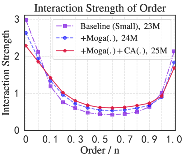
Figure 7: Ablation of designed modules on ImageNet-1K. Left: the table ablates the proposed modules by removing each one based on the baseline of MogaNet-S. Right: the figure plots distributions of the interaction strength $J^{(m)}$ and verifies that $\mathrm{Moga}(\cdot)$ contributes the most to learning multi-order interactions and better performance.

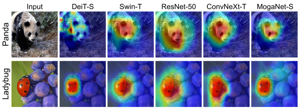
Figure 8: Grad-CAM activation maps on IN-1K. MogaNet shows similar activation maps as local attention architectures (Swin), which are located on the semantic targets. Unlike the results of previous ConvNets, which might activate some irrelevant parts, the activation maps of MogaNet are more gathered. See more results in Appendix B.2.

5.3 Ablation and Analysis

We first ablate the spatial aggregation module in Table 2 and Fig. 7 (left), including FD$(\cdot)$ and Moga$(\cdot)$, which contains the gating branch and the context branch with multi-order DWConv layers Multi-DW$(\cdot)$, and the channel aggregation module CA$(\cdot)$. We found that all proposed modules yield improvements with a few costs. Appendix C provides more ablation studies. Furthermore, we empirically show design modules can learn more middle-order interactions in Fig. 7 (right) and visualize class activation maps (CAM) by Grad-CAM [108] compared to existing models in Fig. 8.

6 Conclusion

In this paper, we present MogaNet, a computationally efficient pure ConvNet architecture from the novel view of multi-order game-theoretic interaction. By paying special attention to multi-order game-theoretic interaction, we design a unified Moga Block, which effectively captures robust multi-order context across spatial and channel spaces. Extensive experiments verify the consistent superiority of MogaNet in terms of accuracy and computational efficiency compared to representative ConvNets, ViTs, and hybrid architectures on various vision benchmarks.

Appendix A Implementation Details

A.1 Architecture Details

The detailed architecture specifications of MogaNet are shown in Table A1 and Fig. A1, where an input image of $224^{2}$ resolutions is assumed for all architectures. We rescale the groups of embedding dimensions the number of Moga Blocks for each stage corresponding to different models of varying magnitudes: i) MogaNet-X-Tiny and MogaNet-Tiny with embedding dimensions of $\{32,64,96,192\}$ and $\{32,64,128,256\}$ exhibit competitive parameter numbers and computational overload as recently proposed light-weight architectures [93, 19, 161]; ii) MogaNet-Small adopts embedding dimensions of $\{64,128,320,512\}$ in comparison to other prevailing small-scale architectures [85, 86]; iii) MogaNet-Base with embedding dimensions of $\{64,160,320,512\}$ in comparison to medium size architectures; iv) MogaNet-Large with embedding dimensions of $\{64,160,320,640\}$ is designed for large-scale computer vision tasks. v) MogaNet-X-Large with embedding dimensions of $\{96,192,480,960\}$ is a scaling-up version (around 200M parameters) for large-scale tasks. The FLOPs are measured for image classification on ImageNet [34] at resolution $224^{2}$, where a global average pooling (GAP) layer is applied to the output feature map of the last stage, followed by a linear classifier.

Stage	Output	Layer	MogaNet
	Size	Settings	XTiny	Tiny	Small	Base	Large	XLarge
S1	$\frac{H\times W}{4\times 4}$	Stem	$\rm{Conv}_{3\times 3},~{}\rm{stride}~{}2,C/2$ $\rm{Conv}_{3\times 3},~{}\rm{stride}~{}2,C$
		Embed. Dim.	32	32	64	64	64	96
		# Moga Block	3	3	2	4	4	6
		MLP Ratio	8
S2	$\frac{H\times W}{8\times 8}$	Stem	$\rm{Conv}_{3\times 3},\rm{stride}~{}2$
		Embed. Dim.	64	64	128	160	160	192
		# Moga Block	3	3	3	6	6	6
		MLP Ratio	8
S3	$\frac{H\times W}{16\times 16}$	Stem	$\rm{Conv}_{3\times 3},~{}\rm{stride}~{}2$
		Embed. Dim.	96	128	320	320	320	480
		# Moga Block	10	12	12	22	44	44
		MLP Ratio	4
S4	$\frac{H\times W}{32\times 32}$	Stem	$\rm{Conv}_{3\times 3},~{}\rm{stride}~{}2$
		Embed. Dim.	192	256	512	512	640	960
		# Moga Block	2	2	2	3	4	4
		MLP Ratio	4
Classifier			Global Average Pooling, Linear
Parameters (M)			2.97	5.20	25.3	43.8	82.5	180.8
FLOPs (G)			0.80	1.10	4.97	9.93	15.9	34.5

Table A1: Architecture configurations of MogaNet variants.

Configuration	DeiT	RSB	MogaNet
		A2	XT	T	S	B	L	XL
Input resolution	2242	2242	2242
Epochs	300	300	300
Batch size	1024	2048	1024
Optimizer	AdamW	LAMB	AdamW
AdamW $(\beta_{1},\beta_{2})$	$(0.9,0.999)$	-	$(0.9,0.999)$
Learning rate	0.001	0.005	0.001
Learning rate decay	Cosine	Cosine	Cosine
Weight decay	0.05	0.02	0.03	0.04	0.05	0.05	0.05	0.05
Warmup epochs	5	5	5
Label smoothing $\epsilon$	0.1	0.1	0.1
Stochastic Depth	✓	✓	0.05	0.1	0.1	0.2	0.3	0.4
Rand Augment	9/0.5	7/0.5	7/0.5	7/0.5	9/0.5	9/0.5	9/0.5	9/0.5
Repeated Augment	✓	✓	✗
Mixup $\alpha$	0.8	0.1	0.1	0.1	0.8	0.8	0.8	0.8
CutMix $\alpha$	1.0	1.0	1.0
Erasing prob.	0.25	✗	0.25
ColorJitter	✗	✗	✗	✗	0.4	0.4	0.4	0.4
Gradient Clipping	✓	✗	✗
EMA decay	✓	✗	✗	✗	✓	✓	✓	✓
Test crop ratio	0.875	0.95	0.90

Table A2: Hyper-parameters for ImageNet-1K training of DeiT, RSB A2, and MogaNet.

A.2 Experimental Settings for ImageNet

We conduct image classification experiments on ImageNet [34] datasets. All experiments are implemented on OpenMixup [74] and timm [138] codebases running on 8 NVIDIA A100 GPUs. View more results in Appendix D.1.

ImageNet-1K.

We perform regular ImageNet-1K training mostly following the training settings of DeiT [122] and RSB A2 [138] in Table A2, which are widely adopted for Transformer and ConvNet architectures. For all models, the default input image resolution is $224^{2}$ for training from scratch. We adopt $256^{2}$ resolutions for lightweight experiments according to MobileViT [93]. Taking training settings for the model with 25M or more parameters as the default, we train all MogaNet models for 300 epochs by AdamW [89] optimizer using a batch size of 1024, a basic learning rate of $1\times 10^{-3}$, a weight decay of 0.05, and a Cosine learning rate scheduler [88] with 5 epochs of linear warmup [35]. As for augmentation and regularization techniques, we adopt most of the data augmentation and regularization strategies applied in DeiT training settings, including Random Resized Crop (RRC) and Horizontal flip [117], RandAugment [28], Mixup [160], CutMix [158], random erasing [164], ColorJitter [53], stochastic depth [62], and label smoothing [118]. Similar to ConvNeXt [86], we do not apply Repeated augmentation [57] and gradient clipping, which are designed for Transformers but do not enhance the performances of ConvNets, while using Exponential Moving Average (EMA) [101] with the decay rate of 0.9999 by default. We also remove additional augmentation strategies [27, 84, 73, 83], e.g., PCA lighting [70] and AutoAugment [27]. Since lightweight architectures (3$\sim$10M parameters) tend to get under-fitted with strong augmentations and regularization, we adjust the training configurations for MogaNet-XT/T following [93, 19, 161], including employing the weight decay of 0.03 and 0.04, Mixup with $\alpha$ of 0.1, and RandAugment of $7/0.5$ for MogaNet-XT/T. Since EMA is proposed to stabilize the training process of large models, we also remove it for MogaNet-XT/T as a fair comparison. An increasing degree of stochastic depth path augmentation is employed for larger models. In evaluation, the top-1 accuracy using a single crop with a test crop ratio of 0.9 is reported as [156, 154, 48].

Configuration	IN-21K PT				IN-1K FT
	S	B	L	XL	S	B	L	XL
Input resolution	2242				3842
Epochs	90				30
Batch size	1024				512
Optimizer	AdamW				AdamW
AdamW $(\beta_{1},\beta_{2})$	$(0.9,0.999)$				$(0.9,0.999)$
Learning rate	$1\times 10^{-3}$				$5\times 10^{-5}$
Learning rate decay	Cosine				Cosine
Weight decay	0.05				0.05
Warmup epochs	5				0
Label smoothing $\epsilon$	0.2				0.1	0.1	0.2	0.2
Stochastic Depth	0	0.1	0.1	0.1	0.4	0.6	0.7	0.8
Rand Augment	9/0.5				9/0.5
Repeated Augment	✗				✗
Mixup $\alpha$	0.8				✗
CutMix $\alpha$	1.0				✗
Erasing prob.	0.25				0.25
ColorJitter	0.4				0.4
Gradient Clipping	✗				✗
EMA decay	✗				✓
Test crop ratio	0.90				1.0

Table A3: Detailed training recipe for ImageNet-21K pre-training (IN-21K PT) and ImageNet-1K fine-tuning (IN-1K FT) in high resolutions for MogaNet.

ImageNet-21K.

Following ConvNeXt, we further provide the training recipe for ImageNet-21K [34] pre-training and ImageNet-1K fine-tuning with high resolutions in Table A3. EMA is removed in pre-training, while CutMix and Mixup are removed for fine-tuning.

A.3 Object Detection and Segmentation on COCO

Following Swin [85] and PoolFormer [154], we evaluate objection detection and instance segmentation tasks on COCO [81] benchmark, which include 118K training images (train2017) and 5K validation images (val2017). We adopt Mask-RCNN [52] as the standard detectors and use ImageNet-1K pre-trained weights as the initialization of the backbones. We employ AdamW [89] optimizer for training $1\times$ schedulers (12 epochs) with a basic learning rate of $1\times 10^{-4}$ and a batch size of 16. The pre-trained weights on ImageNet-1K and ImageNet-21K are used accordingly to initialise backbones. The shorter side of training images is resized to 800 pixels, and the longer side is resized to not more than 1333 pixels. We calculate the FLOPs of compared models at $800\times 1280$ resolutions. Experiments of COCO detection are implemented on MMDetection [17] codebase and run on 8 NVIDIA A100 GPUs. View detailed results in Appendix D.2.

A.4 Semantic Segmentation on ADE20K

We evaluate semantic segmentation on ADE20K [165] benchmark, which contains 20K training images and 2K validation images, covering 150 fine-grained semantic categories. We first adopt Semantic FPN [69] following PoolFormer [154] and Uniformer [72], which train models for 80K iterations by AdamW [89] optimizer with a basic learning rate of $2\times 10^{-4}$, a batch size of 16, and a poly learning rate scheduler. Then, we utilize UperNet [146] following Swin [85], which employs AdamW optimizer using a basic learning rate of $6\times 10^{-5}$, a weight decay of 0.01, a poly scheduler with a linear warmup of 1,500 iterations. We use ImageNet-1K and ImageNet-21K pre-trained weights to initialize the backbones accordingly. The training images are resized to $512^{2}$ resolutions, and the shorter side of testing images is resized to 512 pixels. We calculate the FLOPs of models at $800\times 2048$ resolutions. Experiments of ADE20K segmentation are implemented on MMSegmentation [24] codebase and run on 8 NVIDIA A100 GPUs. View full comparison results in Appendix D.3.

A.5 2D Human Pose Estimation on COCO

We evaluate 2D human keypoints estimation tasks on COCO [81] benchmark based on Top-Down SimpleBaseline [145] (adding a Top-Down estimation head after the backbone) following PVT [135] and UniFormer [72]. We fine-tune all models for 210 epochs with Adam optimizer [68] using a basic learning rate selected in {$1\times 10^{-3},5\times 10^{-4}$}, a multi-step learning rate scheduler decay at 170 and 200 epochs. ImageNet-1K pre-trained weights are used as the initialization of the backbones. The training and testing images are resized to $256\times 192$ or $384\times 288$ resolutions, and the FLOPs of models are calculated at both resolutions. Experiments of COCO pose estimation are implemented on MMPose [25] codebase and run on 8 NVIDIA A100 GPUs. View full experiment results in Appendix D.4.

A.6 3D Human Pose Estimation

We evaluate MogaNet and popular architectures with 3D human pose estimation tasks with a single monocular image based on ExPose [22]. We first benchmark widely-used ConvNets with the 3D face mesh surface estimation task based on ExPose. All models are trained for 100 epochs on Flickr-Faces-HQ Dataset (FFHQ) [67] and tested on Stirling/ESRC 3D dataset [41], which consists of facial RGB images with ground-truth 3D face scans. 3D Root Mean Square Error (3DRMSE) measures errors between the predicted and ground-truth face scans. Following ExPose, the Adam optimizer is employed with a batch size of 256, a basic learning rate selected in {$2\times 10^{-4},1\times 10^{-4}$}, a multi-step learning rate scheduler decay at 60 and 100 epochs. ImageNet-1K pre-trained weights are adopted as the backbone initialization. The training and testing images are resized to $256\times 256$ resolutions. Then, we evaluate ConvNets with the hand 3D pose estimation tasks. FreiHAND dataset [169], which contains multi-view RGB hand images, 3D MANO hand pose and shape annotations, is adopted for training and testing. Mean Per-Joint Position Error (PA-MPJPE) is used to evaluate 3D skeletons. Notice that a “PA” prefix denotes that the metric measures error after solving rotation, scaling, and translation transforms using Procrustes Alignment. Refer to ExPose for more implementation details. All models use the same training settings as the 3D face task, and the training and testing resolutions are $224\times 224$. Experiments of 3D pose estimation are implemented on MMHuman3D [26] codebase and run on 4 NVIDIA A100 GPUs. View full results in Appendix D.5.

A.7 Video Prediction on Moving MNIST

We evaluate various Metaformer architectures [154] and MogaNet with video prediction tasks on Moving MNIST (MMNIST) [81] based on SimVP [42]. Notice that the hidden translator of SimVP is a 2D network module to learn spatio-temporal representation, which any 2D architecture can replace. Therefore, we can benchmark various architectures based on the SimVP framework. In MMNIST [115], each video is randomly generated with 20 frames containing two digits in $64\times 64$ resolutions, and the model takes 10 frames as the input to predict the next 10 frames. Video predictions are evaluated by Mean Square Error (MSE), Mean Absolute Error (MAE), and Structural Similarity Index (SSIM). All models are trained on MMNIST from scratch for 200 or 2000 epochs with Adam optimizer, a batch size of 16, a OneCycle learning rate scheduler, an initial learning rate selected in {$1\times 10^{-2},5\times 10^{-3},1\times 10^{-3},5\times 10^{-4}$}. Experiments of video prediction are implemented on SimVPv2 codebase and run on a single NVIDIA Tesla V100 GPU. View full benchmark results in Appendix D.6.

Appendix B Empirical Experiment Results

B.1 Representation Bottleneck of DNNs from the View of Multi-order Interaction

Multi-order game-theoretic interaction.

In Sec. 3, we interpret the learned representation of DNNs through the lens of multi-order game-theoretic interaction [162, 33], which disentangles inter-variable communication effects in a DNN into diverse game-theoretic components of different interaction orders. The order here denotes the scale of context involved in the whole computation process of game-theoretic interaction.

For computer vison, the $m$-th order interaction $I^{(m)}(i,j)$ measures the average game-theoretic interaction effects between image patches $i$ and $j$ on all $m$ image patches contexts. Take face recognition as an example, we can consider patches $i$ and $j$ as two eyes on this face. Besides, we regard other $m$ visible image patches included on the face. The interaction effect and contribution between eyes pathces $i$ and $j$ toward the task depends on such $m$ visible patches as the context, which is measured as the aforementioned $I^{(m)}(i,j)$. If $I^{(m)}(i,j)>0$ , patches $i$ and $j$ show a positive effect under $m$ context. Accordingly, if $I^{(m)}(i,j)<0$, we consider$i$ and $j$ have a negative effect under $m$ context. More importantly, interactions of low-order mainly reflect widely-shared local texture and common visual concepts. The middle-order interactions are primarily responsible for encoding discriminative high-level representations. However, the high-order ones are inclined to let DNNs memorize the pattern of rare outliers and large-scale shape with intensive global interactions, which can presumably over-fit our deep models [33, 20]. Consequently, the occurrence of excessively low- or high-order game-theoretic interaction in a deep archtecture may therefore undesirable.

Formally, given an input image $x$ with a set of $n$ patches $N=\{1,\dots,n\}$ (e.g., an image with $n$ pixels in total), the multi-order interaction $I^{(m)}(i,j)$ can be calculated as:

$$I^{(m)}(i,j)=\mathbb{E}_{S\subseteq N\setminus\{i,j\},|S|=m}[\Delta f(i,j,S)],$$ (11)

where $\Delta f(i,j,S)=f(S\cup\{i,j\})-f(S\cup\{i\})-f(S\cup\{j\})+f(S)$. $f(S)$ indicates the score of output with patches in $N\setminus S$ kept unchanged but replaced with the baseline value [2], For example, a low-order interaction (e.g., $m=0.05n$) means the relatively simple collaboration between variables $i,j$ under a small range of context, while a high-order interaction (e.g., $m=0.95n$) corresponds to the complex collaboration under a large range of context. Then, we can measure the overall interaction complexity of deep neural networks (DNNs) by the relative interaction strength $J^{(m)}$ of the encoded $m$-th order interaction:

$$J^{(m)}=\frac{\mathbb{E}_{x\in\Omega}\mathbb{E}_{i,j}|I^{(m)}(i,j|x)|}{\mathbb{E}_{m^{{}^{\prime}}}\mathbb{E}_{x\in\Omega}\mathbb{E}_{i,j}|I^{(m^{{}^{\prime}})}(i,j|x)|},$$ (12)

where $\Omega$ is the set of all samples and $0\leq m\geq n-2$. Note that $J^{(m)}$ is the average interaction strength over all possible patch pairs of the input samples and indicates the distribution (area under curve sums up to one) of the order of interactions of DNNs. In Fig. 3, we calculate the interaction strength $J^{(m)}$ with Eq. 12 for the models trained on ImageNet-1K using the official implementation provided by [33]. Specially, we use the image of $224\times 224$ resolution as the input and calculate $J^{(m)}$ on $14\times 14$ grids, i.e., $n=14\times 14$. And we set the model output as $f(x_{S})=\log\frac{P(\hat{y}=y|x_{S})}{1-P(\hat{y}=y|x_{S})}$ given the masked sample $x_{S}$, where $y$ denotes the ground-truth label and $P(\hat{y}=y|x_{S})$ denotes the probability of classifying the masked sample $x_{S}$ to the true category.

Relationship of explaining works of ViTs.

Since the thriving of ViTs in a wide range of computer vision tasks, recent studies mainly investigate the why ViTs work from two directions: (a) Evaluation of robustness against noises finds that self-attentions [94, 97, 167, 75] or gating mechanisms [166] in ViTs are more robust than classical convolutional operations [113, 118]. For example, ViTs can still recognize the target object with large occlusion ratios (e.g., only 10$\sim$20% visible patches) or corruption noises. This phenomenon might stem from the inherent redundancy of images and the competition property of self-attention mechanisms [134, 140]. Several recently proposed works [152, 45] show that ViTs can work with some essential tokens (e.g., 5$\sim$50%) that are selected according to the complexity of input images by dynamic sampling strategies, which also utilize the feature selection properties of self-attentions. From the perspective of multi-order interactions, convolutions with local inductive bias (using small kernel sizes) prefer low-order interactions, while self-attentions without any inductive bias tend to learn low-order and high-order interactions. (b) Evaluation of out-of-distribution samples reveals that both self-attention mechanisms and depth-wise convolution (DWConv) with large kernel designs share similar shape-bias tendency as human vision [128, 43, 36], while canonical ConvNets (using convolutions with small kernel sizes) exhibit strong bias on local texture [44, 56]. Current works [36] attribute shape or texture-bias tendency to the receptive field of self-attention or convolution operations, i.e., an operation with the larger receptive field or more long-range dependency is more likely to be shape-bias. However, there are still gaps between shape-bias operations and human vision. Human brains [126, 33] attain visual patterns and clues and conduct middle-complexity interactions to recognize objects, while a self-attention or convolution operation can only encode global or local features to conduct high or low-complexity interactions. As the existing design of DNNs only stacks regionality perception or context aggregation operations in a cascaded way, it is inevitable to encounter the representation bottleneck.

B.2 Visualization of CAM

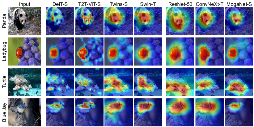
Figure A3: Visualization of Grad-CAM activation maps of the models trained on ImageNet-1K.

We further visualize more examples of Grad-CAM [108] activation maps of MogaNet-S in comparison to Transformers, including DeiT-S [122], T2T-ViT-S [156], Twins-S [23], and Swin [85], and ConvNets, including ResNet-50 [53] and ConvNeXt-T [86], on ImageNet-1K in Fig. A3. Due to the self-attention mechanism, the pure Transformers architectures (DeiT-S and T2T-ViT-S) show more refined activation maps than ConvNets, but they also activate some irrelevant parts. Combined with the design of local windows, local attention architectures (Twins-S and Swin-T) can locate the full semantic objects. Results of previous ConvNets can roughly localize the semantic target but might contain some background regions. The activation parts of our proposed MogaNet-S are more similar to local attention architectures than previous ConvNets, which are more gathered on the semantic objects.

Appendix C More Ablation and Analysis Results

In addition to Sec. 5.3, we further conduct more ablation and analysis of our proposed MogaNet on ImageNet-1K. We adopt the same experimental settings as Sec. 2.

C.1 Ablation of Activation Functions

We conduct the ablation of activation functions used in the proposed multi-order gated aggregation module on ImageNet-1K. Table A4 shows that using SiLU [39] activation for both branches achieves the best performance. Similar results were also found in Transformers, e.g., GLU variants with SiLU or GELU [54] yield better performances than using Sigmoid or Tanh activation functions [109, 61]. We assume that SiLU is the most suitable activation because it owns both the property of Sigmoid (gating effects) and GELU (training friendly), which is defined as $x\cdot\mathrm{Sigmoid}(x)$.

Top-1		Context branch
	Acc (%)	None	GELU	SiLU
	None	76.3	76.7	76.7
Gating	Sigmoid	76.8	77.0	76.9
branch	GELU	76.7	76.8	77.0
	SiLU	76.9	77.1	77.2

Table A4: Ablation of activation functions for the gating and context branches in the $\mathrm{Moga}(\cdot)$ module.

Modules	Top-1	Params.	FLOPs
	Acc (%)	(M)	(G)
Baseline (+Gating branch)	77.2	5.09	1.070
$\mathrm{DW}_{7\times 7}$	77.4	5.14	1.094
$\mathrm{DW}_{5\times 5,d=1}+\mathrm{DW}_{7\times 7,d=3}$	77.5	5.15	1.112
$\mathrm{DW}_{5\times 5,d=1}+\mathrm{DW}_{5\times 5,d=2}+\mathrm{DW}_{7\times 7,d=3}$	77.5	5.17	1.185
+Multi-order, $C_{l}:C_{m}:C_{h}=1:0:3$	77.5	5.17	1.099
+Multi-order, $C_{l}:C_{m}:C_{h}=0:1:1$	77.6	5.17	1.103
+Multi-order, $C_{l}:C_{m}:C_{h}=1:6:9$	77.7	5.17	1.104
+Multi-order, $C_{l}:C_{m}:C_{h}=1:3:4$	77.8	5.17	1.102

Table A5: Ablation of multi-order DWConv layers in the proposed $\mathrm{Moga}(\cdot)$ module. The baseline adopts the MogaNet framework using the non-linear projection, $\mathrm{DW}_{5\times 5}$, and the SiLU gating branch as $\mathrm{SMixer}(\cdot)$ and using the vanilla MLP as $\mathrm{CMixer}(\cdot)$.

C.2 Ablation of Multi-order DWConv Layers

In addition to Sec. 4.2 and Sec. 5.3, we also analyze the multi-order depth-wise convolution (DWConv) layers as the static regionality perception in the multi-order aggregation module $\mathrm{Moga}(\cdot)$ on ImageNet-1K. As shown in Table A5, we analyze the channel configuration of three parallel dilated DWConv layers: $\mathrm{DW}_{5\times 5,d=1}$, $\mathrm{DW}_{5\times 5,d=2}$, and $\mathrm{DW}_{7\times 7,d=3}$ with the channels of $C_{l}$, $C_{m}$, $C_{h}$. we first compare the performance of serial DWConv layers (e.g., $\mathrm{DW}_{5\times 5,d=1}$+$\mathrm{DW}_{7\times 7,d=3}$) and parallel DWConv layers. We find that the parallel design can achieve the same performance with fewer computational overloads because the DWConv kernel is equally applied to all channels. When we adopt three DWConv layers, the proposed parallel design reduces $C_{l}+C_{h}$ and $C_{l}+C_{m}$ times computations of $\mathrm{DW}_{5\times 5,d=2}$ and $\mathrm{DW}_{5\times 5,d=2}$ in comparison to the serial stack of these DWConv layers. Then, we empirically explore the optimal configuration of the three channels. We find that $C_{l}:$ $C_{m}:$ $C_{h}$ = 1: 3: 4 yields the best performance, which well balances the small, medium, and large DWConv kernels to learn low, middle, and high-order contextual representations. We calculate and discuss the FLOPs of the proposed three DWConv layers in the next subsection to verify the efficiency. Similar conclusions are also found in relevant designs [95, 111, 105], where global context aggregations take the majority (e.g., $\frac{1}{2}\sim\frac{3}{4}$ channels or context components). We also verify the parallel design with the optimal configuration based on MogaNet-S/B. Therefore, we can conclude that our proposed multi-order DWConv layers can efficiently learn multi-order contextual information for the context branch of $\mathrm{Moga}(\cdot)$.

C.3 FLOPs and Throughputs of MogaNet

FLOPs of Multi-order Gated Aggregation Module

We divide the computation of the proposed multi-order gated aggregation module into two parts of convolution operations and calculate the FLOPs for each part.

• Conv1$\times$1. The FLOPs of 1$\times$1 convolution operation $\phi_{\rm gate}$ , $\phi_{\rm context}$ and $\phi_{\rm out}$ can be derived as:

  $$\mathrm{FLOPs}(\phi_{\rm gate}) =2HWC^{2},$$ (13)

  $$\mathrm{FLOPs}(\phi_{\rm context}) =2HWC^{2},$$

  $$\mathrm{FLOPs}(\phi_{\rm out}) =2HWC^{2}.\vspace{-0.50em}$$

• Depth-wise convolution. We consider the depth-wise convolution ($\mathrm{DW}$) with dilation ratio $d$. The $\mathrm{DW}$Conv is performed for the input $X$, where $X\in\mathbb{R}^{HW\times C_{in}}$. Therefore, the FLOPs for all $\mathrm{DW}$ in Moga module are:

  $$\mathrm{FLOPs}(\mathrm{DW}_{5\times 5,d=1}) =2HWC_{in}K_{5\times 5}^{2},$$ (14)

  $$\mathrm{FLOPs}(\mathrm{DW}_{5\times 5,d=2}) =\frac{3}{4}HWC_{in}K_{5\times 5}^{2},$$

  $$\mathrm{FLOPs}(\mathrm{DW}_{7\times 7,d=3}) =HWC_{in}K_{7\times 7}^{2}.\vspace{-0.50em}$$

Overall, the total FLOPs of our Moga module can be derived as follows:

$$\mathrm{FLOPs}(\mathrm{Moga}) =2HWC_{in}\left[\frac{11}{8}K_{5\times 5}^{2}+\frac{1}{2}K_{7\times 7}^{2}+3C_{in}\right]$$ (15)

$$=HWC_{in}\left[\frac{471}{4}+6C_{in}\right].\vspace{-0.5em}$$

Throughput of MogaNet

We further analyze throughputs of MogaNet variants on ImageNet-1K. As shown in Fig. A2, MogaNet has similar throughputs as Swin Transformer while producing better performances than Swin and ConvNet. Since we add channel splitting and GAP operations in MogaNet, the throughput of ConvNeXt exceeds MogaNet to some extent.

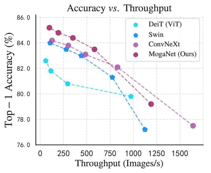
Figure A2: Accuracy-throughput diagram of models on ImageNet-1K measured on an NVIDIA Tesla V100 GPU.

C.4 Ablation of Normalization Layers

For most of ConvNets, BatchNorm [64] (BN) is considered an essential component to improve the convergence speed and prevent overfitting. However, BN might cause some instability [144] or harm the final performance of models [8, 9]. Some recently proposed ConvNets [86, 48] replace BN by LayerNorm [4] (LN), which has been widely used in Transformers [38] and Metaformer architectures [154], achieving relatively good performances in various scenarios. Here, we conduct an ablation of normalization (Norm) layers in MogaNet on ImageNet-1K, as shown in Table A6. As discussed in ConvNeXt [86], the Norm layers used in each block (within) and after each stage (after) have different effects. Thus we study them separately. Table A6 shows that using BN in both places yields better performance than using LN (after) and BN (within), except MogaNet-T with $224^{2}$ resolutions, while using LN in both places performs the worst. Consequently, we use BN as the default Norm layers in our proposed MogaNet for two reasons: (i) With pure convolution operators, the rule of combining convolution operations with BN within each stage is still useful for modern ConvNets. (ii) Although using LN after each stage might help stabilize the training process of Transformers and hybrid models and might sometimes bring good performance for ConvNets, adopting BN after each stage in pure convolution models still yields better performance. Moreover, we replace BN with precise BN [144] (pBN), which is an optimal alternative normalization strategy to BN. We find slight performance improvements (around 0.1%), especially when MogaNet-S/B adopts the EMA strategy (by default), indicating that we can further improve MogaNet with advanced BN. As discussed in ConvNeXt, EMA might severely hurt the performances of models with BN. This phenomenon might be caused by the unstable and inaccurate BN statistics estimated by EMA in the vanilla BN with large models, which will deteriorate when using another EMA of model parameters. We solve this dilemma by exponentially increasing the EMA decay from 0.9 to 0.9999 during training as momentum-based contrastive learning methods [15, 7], e.g., BYOL [46]. It can also be tackled by advanced BN variants [58, 144].

Norm (after)	Input	LN	LN	BN	pBN
Norm (within)	size	LN	BN	BN	pBN
MogaNet-T	2242	78.4	79.1	79.0	79.1
MogaNet-T	2562	78.8	79.4	79.6	79.6
MogaNet-S	2242	82.5	83.2	83.3	83.3
MogaNet-S (EMA)	2242	82.7	83.2	83.3	83.4
MogaNet-B	2242	83.4	83.9	84.1	84.2
MogaNet-B (EMA)	2242	83.7	83.8	84.3	84.4

Table A6: Ablation of normalization layers in MogaNet.

C.5 Refined Training Settings for Lightweight Models

To explore the full power of lightweight models of our MogaNet, we refined the basic training settings for MogaNet-XT/T according to RSB A2 [138] and DeiT-III [125]. Compared to the default setting as provided in Table A2, we only adjust the learning rate and the augmentation strategies for faster convergence while keeping other settings unchanged. As shown in Table A7, MogaNet-XT/T gain +0.4$\sim$0.6% when use the large learning rate of $2\times 10^{-3}$ and 3-Augment [125] without complex designs. Based on the advanced setting, MogaNet with $224^{2}$ input resolutions yields significant performance improvements against previous methods, e.g., MogaNet-T gains +3.5% over DeiT-T [122] and +1.2% over Parc-Net-S [161]. Especially, MogaNet-T with $256^{2}$ resolutions achieves top-1 accuracy of 80.0%, outperforming DeiT-S of 79.8% reported in the original paper, while MogaNet-XT with $224^{2}$ resolutions outperforms DeiT-T under the refined training scheme by 1.2% with only 3M parameters.

Architecture	Input	Learning	Warmup	Rand	3-Aug	EMA	Top-1
	size	rate	epochs	Augment	[125]		Acc (%)
DeiT-T [122]	$224^{2}$	$1\times 10^{-3}$	5	9/0.5	✗	✓	72.2
DeiT-T [122]	$224^{2}$	$2\times 10^{-3}$	20	✗	✓	✗	75.9
ParC-Net-S [161]	$256^{2}$	$1\times 10^{-3}$	5	9/0.5	✗	✓	78.6
ParC-Net-S [161]	$256^{2}$	$2\times 10^{-3}$	20	✗	✓	✗	78.8
MogaNet-XT	$224^{2}$	$1\times 10^{-3}$	5	7/0.5	✗	✗	76.5
MogaNet-XT	$224^{2}$	$2\times 10^{-3}$	20	✗	✓	✗	77.1
MogaNet-XT	$256^{2}$	$1\times 10^{-3}$	5	7/0.5	✗	✗	77.2
MogaNet-XT	$256^{2}$	$2\times 10^{-3}$	20	✗	✓	✗	77.6
MogaNet-T	$224^{2}$	$1\times 10^{-3}$	5	7/0.5	✗	✗	79.0
MogaNet-T	$224^{2}$	$2\times 10^{-3}$	20	✗	✓	✗	79.4
MogaNet-T	$256^{2}$	$1\times 10^{-3}$	5	7/0.5	✗	✗	79.6
MogaNet-T	$256^{2}$	$2\times 10^{-3}$	20	✗	✓	✗	80.0

Table A7: Advanced training recipes for Lightweight models of MogaNet on ImageNet-1K.

Architecture	Type	#P.	FLOPs	RetinaNet $1\times$
		(M)	(G)	AP	AP50	AP75	APS	APM	APL
RegNet-800M [103]	C	17	168	35.6	54.7	37.7	19.7	390	47.8
PVTV2-B0 [136]	T	13	160	37.1	57.2	39.2	23.4	40.4	49.2
MogaNet-XT	C	12	167	39.7	60.0	42.4	23.8	43.6	51.7
ResNet-18 [53]	C	21	189	31.8	49.6	33.6	16.3	34.3	43.2
RegNet-1.6G [103]	C	20	185	37.4	56.8	39.8	22.4	41.1	49.2
RegNet-3.2G [103]	C	26	218	39.0	58.4	41.9	22.6	43.5	50.8
PVT-T [135]	T	23	183	36.7	56.9	38.9	22.6	38.8	50.0
PoolFormer-S12 [154]	T	22	207	36.2	56.2	38.2	20.8	39.1	48.0
PVTV2-B1 [136]	T	24	187	41.1	61.4	43.8	26.0	44.6	54.6
MogaNet-T	C	14	173	41.4	61.5	44.4	25.1	45.7	53.6
ResNet-50 [53]	C	37	239	36.3	55.3	38.6	19.3	40.0	48.8
PVT-S [135]	T	34	226	40.4	61.3	43.0	25.0	42.9	55.7
Twins-SVT-S [23]	T	34	209	42.3	63.4	45.2	26.0	45.5	56.5
Focal-T [151]	T	39	265	43.7	-	-	-	-	-
PoolFormer-S36 [154]	T	41	272	39.5	60.5	41.8	22.5	42.9	52.4
PVTV2-B2 [136]	T	35	281	44.6	65.7	47.6	28.6	48.5	59.2
CMT-S [47]	H	45	231	44.3	65.5	47.5	27.1	48.3	59.1
MogaNet-S	C	35	253	45.8	66.6	49.0	29.1	50.1	59.8
ResNet-101 [53]	C	57	315	38.5	57.8	41.2	21.4	42.6	51.1
PVT-M [135]	T	54	258	41.9	63.1	44.3	25.0	44.9	57.6
Focal-S [151]	T	62	367	45.6	-	-	-	-	-
PVTV2-B3 [136]	T	55	263	46.0	67.0	49.5	28.2	50.0	61.3
PVTV2-B4 [136]	T	73	315	46.3	67.0	49.6	29.0	50.1	62.7
MogaNet-B	C	54	355	47.7	68.9	51.0	30.5	52.2	61.7
ResNeXt-101-64 [148]	C	95	473	41.0	60.9	44.0	23.9	45.2	54.0
PVTV2-B5	T	92	335	46.1	66.6	49.5	27.8	50.2	62.0
MogaNet-L	C	92	477	48.7	69.5	52.6	31.5	53.4	62.7

Table A8: Object detection with RetinaNet ($1\times$ training schedule) on COCO val2017. The FLOPs are measured at resolution $800\times 1280$.

Architecture	Type	#P.	FLOPs	Mask R-CNN $1\times$
		(M)	(G)	APb	AP${}_{50}^{b}$	AP${}_{75}^{b}$	APm	AP${}_{50}^{m}$	AP${}_{75}^{m}$
RegNet-800M [103]	C	27	187	37.5	57.9	41.1	34.3	56.0	36.8
MogaNet-XT	C	23	185	40.7	62.3	44.4	37.6	59.6	40.2
ResNet-18 [53]	C	31	207	34.0	54.0	36.7	31.2	51.0	32.7
RegNet-1.6G [103]	C	29	204	38.9	60.5	43.1	35.7	57.4	38.9
PVT-T [135]	T	33	208	36.7	59.2	39.3	35.1	56.7	37.3
PoolFormer-S12 [154]	T	32	207	37.3	59.0	40.1	34.6	55.8	36.9
MogaNet-T	C	25	192	42.6	64.0	46.4	39.1	61.3	42.0
ResNet-50 [53]	C	44	260	38.0	58.6	41.4	34.4	55.1	36.7
RegNet-6.4G [103]	C	45	307	41.1	62.3	45.2	37.1	59.2	39.6
PVT-S [135]	T	44	245	40.4	62.9	43.8	37.8	60.1	40.3
Swin-T [85]	T	48	264	42.2	64.6	46.2	39.1	61.6	42.0
MViT-T [40]	T	46	326	45.9	68.7	50.5	42.1	66.0	45.4
PoolFormer-S36 [154]	T	32	207	41.0	63.1	44.8	37.7	60.1	40.0
Focal-T [151]	T	49	291	44.8	67.7	49.2	41.0	64.7	44.2
PVTV2-B2 [136]	T	45	309	45.3	67.1	49.6	41.2	64.2	44.4
LITV2-S [95]	T	47	261	44.9	67.0	49.5	40.8	63.8	44.2
CMT-S [47]	H	45	249	44.6	66.8	48.9	40.7	63.9	43.4
Conformer-S/16 [99]	H	58	341	43.6	65.6	47.7	39.7	62.6	42.5
Uniformer-S [72]	H	41	269	45.6	68.1	49.7	41.6	64.8	45.0
ConvNeXt-T [86]	C	48	262	44.2	66.6	48.3	40.1	63.3	42.8
FocalNet-T (SRF)[150]	C	49	267	45.9	68.3	50.1	41.3	65.0	44.3
FocalNet-T (LRF)[150]	C	49	268	46.1	68.2	50.6	41.5	65.1	44.5
MogaNet-S	C	45	272	46.7	68.0	51.3	42.2	65.4	45.5
ResNet-101 [53]	C	63	336	40.4	61.1	44.2	36.4	57.7	38.8
RegNet-12G [103]	C	64	423	42.2	63.7	46.1	38.0	60.5	40.5
PVT-M [135]	T	64	302	42.0	64.4	45.6	39.0	61.6	42.1
Swin-S [85]	T	69	354	44.8	66.6	48.9	40.9	63.4	44.2
Focal-S [151]	T	71	401	47.4	69.8	51.9	42.8	66.6	46.1
PVTV2-B3 [136]	T	65	397	47.0	68.1	51.7	42.5	65.7	45.7
LITV2-M [95]	T	68	315	46.5	68.0	50.9	42.0	65.1	45.0
UniFormer-B [72]	H	69	399	47.4	69.7	52.1	43.1	66.0	46.5
ConvNeXt-S [86]	C	70	348	45.4	67.9	50.0	41.8	65.2	45.1
MogaNet-B	C	63	373	47.9	70.0	52.7	43.2	67.0	46.6
Swin-B [85]	T	107	496	46.9	69.6	51.2	42.3	65.9	45.6
PVTV2-B5 [136]	T	102	557	47.4	68.6	51.9	42.5	65.7	46.0
ConvNeXt-B [86]	C	108	486	47.0	69.4	51.7	42.7	66.3	46.0
FocalNet-B (SRF)[150]	C	109	496	48.8	70.7	53.5	43.3	67.5	46.5
MogaNet-L	C	102	495	49.4	70.7	54.1	44.1	68.1	47.6

Table A9: Object detection and instance segmentation with Mask R-CNN ($1\times$ training schedule) on COCO val2017. The FLOPs are measured at resolution $800\times 1280$.

Appendix D More Comparison Experiments

D.1 Fast Training on ImageNet-1K

In addition to Sec. 5.1, we further provide comparison results for 100 and 300 epochs training on ImageNet-1K. As for 100-epoch training, we adopt the original RSB A3 [138] setting for all methods, which adopts LAMB [153] optimizer and a small training resolution of $160^{2}$. We search the basic learning in {$0.006,0.008$} for all architectures and adopt the gradient clipping for Transformer-based networks. As for 300-epoch training, we report results of RSB A2 [138] for classical CNN or the original setting for Transformers or modern ConvNets. In Table A15, when compared with models of similar parameter size, our proposed MogaNet-XT/T/S/B achieves the best performance in both 100 and 300 epochs training. Results of 100-epoch training show that MogaNet has a faster convergence speed than previous architectures of various types. For example, MogaNet-T outperforms EfficientNet-B0 and DeiT-T by 2.4% and 8.7%, MogaNet-S outperforms Swin-T by 3.4%, and MogaNet-B outperforms Swin-S by 2.0%. Notice that ConvNeXt variants have a great convergence speed, e.g., ConvNeXt-S achieves 81.7% surpassing Swin-S by 1.5 and recently proposed ConvNet HorNet-S_7×7 by 0.5 with similar parameters. But our proposed MogaNet convergences faster than ConvNet, e.g., MogaNet-S outperforms ConvNeXt-T by 2.3% with similar parameters while MogaNet-B/L reaching competitive performances as ConvNeXt-B/L with only 44$\sim$50% parameters.

D.2 Detection and Segmentation Results on COCO

In addition to Sec. 5.2, we provide full results of object detection and instance segmentation tasks with RetinaNet, Mask R-CNN, and Cascade Mask R-CNN on COCO. As shown in Table A8 and Table A9, RetinaNet or Mask R-CNN with MogaNet variants outperforms existing models when training $1\times$ schedule. For example, RetinaNet with MogaNet-T/S/B/L achieve 45.8/47.7/48.7 AP^b, outperforming PVT-T/S/M and PVTV2-B1/B2/B3/B5 by 4.7/4.6/5.8 and 0.3/1.2/1.7/2.6 AP^b; Nask R-CNN with MogaNet-S/B/L achieve 46.7/47.9/49.4 AP^b, exceeding Swin-T/S/B and ConvNeXt-T/S/B by 4.5/3.1/2.5 and 2.5/2.5/2.4 with similar parameters and computational overloads. Noticeably, MogaNet-XT/T achieve better detection results with fewer parameters and lower FLOPs than lightweight architectures, while MogaNet-T even surpasses some Transformers like Swin-S and PVT-S. For example, Mask R-CNN with MogaNet-T improves Swin-T by 0.4 AP^b and outperforms PVT-S by 1.3 AP^m using only around 2/3 parameters. As shown in Table A10, Cascade Mask R-CNN with MogaNet variants still achieves the state-of-the-art detection and segmentation results when training $3\times$ schedule with multi-scaling (MS) and advanced augmentations. For example, MogaNet-L/XL yield 53.3/56.2 AP^b and 46.1/48.8 AP^m, which improves Swin-B/L and ConvNeXt-B/L by 1.4/2.3 and 0.6/1.4 AP^b with similar parameters and FLOPS.

Architecture	Type	#P.	FLOPs	Cascade Mask R-CNN +MS $3\times$
		(M)	(G)	APbb	AP${}_{50}^{b}$	AP${}_{75}^{b}$	APm	AP${}_{50}^{m}$	AP${}_{75}^{m}$
ResNet-50 [53]	C	77	739	46.3	64.3	50.5	40.1	61.7	43.4
Swin-T [85]	T	86	745	50.4	69.2	54.7	43.7	66.6	47.3
Focal-T [151]	T	87	770	51.5	70.6	55.9	-	-	-
ConvNeXt-T [86]	C	86	741	50.4	69.1	54.8	43.7	66.5	47.3
FocalNet-T (SRF) [150]	C	86	746	51.5	70.1	55.8	44.6	67.7	48.4
MogaNet-S	C	78	750	51.6	70.8	56.3	45.1	68.7	48.8
ResNet-101-32 [53]	C	96	819	48.1	66.5	52.4	41.6	63.9	45.2
Swin-S [85]	T	107	838	51.9	70.7	56.3	45.0	68.2	48.8
ConvNeXt-S [86]	C	108	827	51.9	70.8	56.5	45.0	68.4	49.1
MogaNet-B	C	101	851	52.6	72.0	57.3	46.0	69.6	49.7
Swin-B [85]	T	145	982	51.9	70.5	56.4	45.0	68.1	48.9
ConvNeXt-B [86]	C	146	964	52.7	71.3	57.2	45.6	68.9	49.5
MogaNet-L	C	140	974	53.3	71.8	57.8	46.1	69.2	49.8
Swin-L‡ [85]	T	253	1382	53.9	72.4	58.8	46.7	70.1	50.8
ConvNeXt-L‡ [86]	C	255	1354	54.8	73.8	59.8	47.6	71.3	51.7
ConvNeXt-XL‡ [86]	C	407	1898	55.2	74.2	59.9	47.7	71.6	52.2
RepLKNet-31L‡ [36]	C	229	1321	53.9	72.5	58.6	46.5	70.0	50.6
HorNet-L‡ [105]	C	259	1399	56.0	-	-	48.6	-	-
MogaNet-XL‡	C	238	1355	56.2	75.0	61.2	48.8	72.6	53.3

Table A10: Object detection and instance segmentation with Cascade Mask R-CNN ($3\times$ training schedule) with multi-scaling training (MS) on COCO val2017. ^‡ denotes the model is pre-trained on ImageNet-21K. The FLOPs are measured at resolution $800\times 1280$.

D.3 Sementic Segmentation Results on ADE20K

In addition to Sec. 5.2, we provide comprehensive comparison results of semantic segmentation based on UperNet on ADE20K. As shown in Table A11, UperNet with MogaNet produces state-of-the-art performances in a wide range of parameter scales compared to famous Transformer, hybrid, and convolution models. As for the lightweight models, MogaNet-XT/T significantly improves ResNet-18/50 with fewer parameters and FLOPs budgets. As for medium-scaling models, MogaNet-S/B achieves 49.2/50.1 mIoU^ss, which outperforms the recently proposed ConvNets, e.g., +1.1 over HorNet-T using similar parameters and +0.7 over SLaK-S using 17M fewer parameters. As for large models, MogaNet-L/XL surpass Swin-B/L and ConvNeXt-B/L by 1.2/1.9 and 1.8/0.3 mIoU^ss while using fewer parameters.

Architecture	Date	Type	Crop	Param.	FLOPs	mIoUss
			size	(M)	(G)	(%)
ResNet-18 [53]	CVPR’2016	C	5122	41	885	39.2
MogaNet-XT	Ours	C	5122	30	856	42.2
ResNet-50 [53]	CVPR’2016	C	5122	67	952	42.1
MogaNet-T	Ours	C	5122	33	862	43.7
DeiT-S [122]	ICML’2021	T	5122	52	1099	44.0
Swin-T [85]	ICCV’2021	T	5122	60	945	46.1
TwinsP-S [23]	NIPS’2021	T	5122	55	919	46.2
Twins-S [23]	NIPS’2021	T	5122	54	901	46.2
Focal-T [151]	NIPS’2021	T	5122	62	998	45.8
Uniformer-Sh32 [72]	ICLR’2022	H	5122	52	955	47.0
UniFormer-S [72]	ICLR’2022	H	5122	52	1008	47.6
ConvNeXt-T [86]	CVPR’2022	C	5122	60	939	46.7
FocalNet-T (SRF) [151]	NIPS’2022	C	5122	61	944	46.5
HorNet-T7×7 [105]	NIPS’2022	C	5122	52	926	48.1
MogaNet-S	Ours	C	5122	55	946	49.2
Swin-S [85]	ICCV’2021	T	5122	81	1038	48.1
Twins-B [23]	NIPS’2021	T	5122	89	1020	47.7
Focal-S [151]	NIPS’2021	T	5122	85	1130	48.0
Uniformer-Bh32 [72]	ICLR’2022	H	5122	80	1106	49.5
ConvNeXt-S [86]	CVPR’2022	C	5122	82	1027	48.7
FocalNet-S (SRF) [151]	NIPS’2022	C	5122	83	1035	49.3
SLaK-S [82]	ICLR’2023	C	5122	91	1028	49.4
MogaNet-B	Ours	C	5122	74	1050	50.1
Swin-B [85]	ICCV’2021	T	5122	121	1188	49.7
Focal-B [151]	NIPS’2021	T	5122	126	1354	49.0
ConvNeXt-B [86]	CVPR’2022	C	5122	122	1170	49.1
RepLKNet-31B [36]	CVPR’2022	C	5122	112	1170	49.9
FocalNet-B (SRF) [151]	NIPS’2022	C	5122	124	1180	50.2
SLaK-B [82]	ICLR’2023	C	5122	135	1185	50.2
MogaNet-L	Ours	C	5122	113	1176	50.9
Swin-L‡ [85]	ICCV’2021	T	6402	234	2468	52.1
ConvNeXt-L‡ [86]	CVPR’2022	C	6402	245	2458	53.7
RepLKNet-31L‡ [36]	CVPR’2022	C	6402	207	2404	52.4
MogaNet-XL‡	Ours	C	6402	214	2451	54.0

Table A11: Semantic segmentation with UperNet (160K) on ADE20K validation set. ^‡ indicates using IN-21K pre-trained models. The FLOPs are measured at $512\times 2048$ or $640\times 2560$ resolutions.

D.4 2D Human Pose Estimation Results on COCO

In addition to Sec. 5.2, we provide comprehensive experiment results of 2D human key points estimation based on Top-Down SimpleBaseline on COCO. As shown in Table A13, MogaNet variants achieve competitive or state-of-the-art performances compared to popular architectures with two types of resolutions. As for lightweight models, MogaNet-XT/T significantly improves the performances of existing models while using similar parameters and FLOPs. Meanwhile, MogaNet-S/B also produces 74.9/75.3 and 76.4/77.3 AP using $256\times 192$ and $384\times 288$ resolutions, outperforming Swin-B/L by 2.0/1.0 and 1.5/1.0 AP with nearly half of the parameters and computation budgets.

Architecture		Hand			Face
	Type	#P.	FLOPs	PA-MPJPE	#P.	FLOPs	3DRMSE
		(M)	(G)	(mm)$\downarrow$	(M)	(G)	$\downarrow$
MobileNetV2 [107]	C	4.8	0.3	8.33	4.9	0.4	2.64
ResNet-18 [53]	C	13.0	1.8	7.51	13.1	2.4	2.40
MogaNet-T	C	6.5	1.1	6.82	6.6	1.5	2.36
ResNet-50 [53]	C	26.9	4.1	6.85	27.0	5.4	2.48
ResNet-101 [53]	C	45.9	7.9	6.44	46.0	10.3	2.47
DeiT-S [38]	T	23.4	4.3	7.86	23.5	5.5	2.52
Swin-T [85]	T	30.2	4.6	6.97	30.3	6.1	2.45
Swin-S [85]	T	51.0	13.8	6.50	50.9	8.5	2.48
ConvNeXt-T [86]	C	29.9	4.5	6.18	30.0	5.8	2.34
ConvNeXt-S [86]	C	51.5	8.7	6.04	51.6	11.4	2.27
HorNet-T [105]	C	23.7	4.3	6.46	23.8	5.6	2.39
MogaNet-S	C	26.6	5.0	6.08	26.7	6.5	2.24

Table A12: 3D human pose estimation with ExPose on FFHQ and FreiHAND datasets. The face and hand tasks use pre-vertex and pre-joint errors as the metric. The FLOPs of the face and hand tasks are measured with input images at $256^{2}$ and $224^{2}$ resolutions.

Architecture	Type	Crop	#P.	FLOPs	AP	AP50	AP75	AR
		size	(M)	(G)	(%)	(%)	(%)	(%)
MobileNetV2 [107]	C	$256\times 192$	10	1.6	64.6	87.4	72.3	70.7
ShuffleNetV2 $2\times$ [92]	C	$256\times 192$	8	1.4	59.9	85.4	66.3	66.4
MogaNet-XT	C	$256\times 192$	6	1.8	72.1	89.7	80.1	77.7
RSN-18 [11]	C	$256\times 192$	9	2.3	70.4	88.7	77.9	77.1
MogaNet-T	C	$256\times 192$	8	2.2	73.2	90.1	81.0	78.8
ResNet-50 [53]	C	$256\times 192$	34	5.5	72.1	89.9	80.2	77.6
HRNet-W32 [116]	C	$256\times 192$	29	7.1	74.4	90.5	81.9	78.9
Swin-T [85]	T	$256\times 192$	33	6.1	72.4	90.1	80.6	78.2
PVT-S [135]	T	$256\times 192$	28	4.1	71.4	89.6	79.4	77.3
PVTV2-B2 [136]	T	$256\times 192$	29	4.3	73.7	90.5	81.2	79.1
Uniformer-S [72]	H	$256\times 192$	25	4.7	74.0	90.3	82.2	79.5
ConvNeXt-T [86]	C	$256\times 192$	33	5.5	73.2	90.0	80.9	78.8
MogaNet-S	C	$256\times 192$	29	6.0	74.9	90.7	82.8	80.1
ResNet-101 [53]	C	$256\times 192$	53	12.4	71.4	89.3	79.3	77.1
ResNet-152 [53]	C	$256\times 192$	69	15.7	72.0	89.3	79.8	77.8
HRNet-W48 [116]	C	$256\times 192$	64	14.6	75.1	90.6	82.2	80.4
Swin-B [85]	T	$256\times 192$	93	18.6	72.9	89.9	80.8	78.6
Swin-L [85]	T	$256\times 192$	203	40.3	74.3	90.6	82.1	79.8
Uniformer-B [72]	H	$256\times 192$	54	9.2	75.0	90.6	83.0	80.4
ConvNeXt-S [86]	C	$256\times 192$	55	9.7	73.7	90.3	81.9	79.3
MogaNet-B	C	$256\times 192$	47	10.9	75.3	90.9	83.3	80.7
MobileNetV2 [107]	C	$384\times 288$	10	3.6	67.3	87.9	74.3	72.9
ShuffleNetV2 $2\times$ [92]	C	$384\times 288$	8	3.1	63.6	86.5	70.5	69.7
MogaNet-XT	C	$384\times 288$	6	4.2	74.7	90.1	81.3	79.9
RSN-18 [11]	C	$384\times 288$	9	5.1	72.1	89.5	79.8	78.6
MogaNet-T	C	$384\times 288$	8	4.9	75.7	90.6	82.6	80.9
HRNet-W32 [116]	C	$384\times 288$	29	16.0	75.8	90.6	82.7	81.0
Uniformer-S [72]	H	$384\times 288$	25	11.1	75.9	90.6	83.4	81.4
ConvNeXt-T [86]	C	$384\times 288$	33	33.1	75.3	90.4	82.1	80.5
MogaNet-S	C	$384\times 288$	29	13.5	76.4	91.0	83.3	81.4
ResNet-152 [53]	C	$384\times 288$	69	35.6	74.3	89.6	81.1	79.7
HRNet-W48 [116]	C	$384\times 288$	64	32.9	76.3	90.8	82.0	81.2
Swin-B [85]	T	$384\times 288$	93	39.2	74.9	90.5	81.8	80.3
Swin-L [85]	T	$384\times 288$	203	86.9	76.3	91.2	83.0	814
HRFormer-B [157]	T	$384\times 288$	54	30.7	77.2	91.0	83.6	82.0
ConvNeXt-S [86]	C	$384\times 288$	55	21.8	75.8	90.7	83.1	81.0
Uniformer-B [72]	C	$384\times 288$	54	14.8	76.7	90.8	84.0	81.4
MogaNet-B	C	$384\times 288$	47	24.4	77.3	91.4	84.0	82.2

Table A13: 2D human pose estimation with Top-Down SimpleBaseline on COCO val2017. The FLOPs are measured at $256\times 192$ or $384\times 288$ resolutions.

D.5 3D Human Pose Estimation Results

In addition to Sec. 5.2, we evaluate popular ConvNets and MogaNet for 3D human pose estimation tasks based on ExPose [22]. As shown in Table A12, MogaNet achieves lower regression errors with efficient usage of parameters and computational overheads. Compared to lightweight architectures, MogaNet-T achieves 6.82 MPJPE and 2.36 3DRMSE on hand and face reconstruction tasks, improving ResNet-18 and MobileNetV2 $1\times$ by 1.29/0.04 and 1.51/0.28. Compared to models around 25$\sim$50M parameters, MogaNet-S surpasses ResNet-101 and ConvNeXt-T, achieving competitive results as ConvNeXt-S with relatively smaller parameters and FLOPs (e.g., 27M/6.5G vs 52M/11.4G on FFHP). Notice that some backbones with more parameters produce worse results than their lightweight variants on the face estimation tasks (e.g., ResNet-50 and Swin-S), while MogaNet-S still yields the better performance of 2.24 3DRMSE.

Architecture	#P.	FLOPs	FPS	200 epochs			2000 epochs
	(M)	(G)	(s)	MSE$\downarrow$	MAE$\downarrow$	SSIM$\uparrow$	MSE$\downarrow$	MAE$\downarrow$	SSIM$\uparrow$
ViT [38]	46.1	16.9	290	35.15	95.87	0.9139	19.74	61.65	0.9539
Swin [85]	46.1	16.4	294	29.70	84.05	0.9331	19.11	59.84	0.9584
Uniformer [72]	44.8	16.5	296	30.38	85.87	0.9308	18.01	57.52	0.9609
MLP-Mixer [121]	38.2	14.7	334	29.52	83.36	0.9338	18.85	59.86	0.9589
ConvMixer [127]	3.9	5.5	658	32.09	88.93	0.9259	22.30	67.37	0.9507
Poolformer [154]	37.1	14.1	341	31.79	88.48	0.9271	20.96	64.31	0.9539
SimVP [42]	58.0	19.4	209	32.15	89.05	0.9268	21.15	64.15	0.9536
ConvNeXt [86]	37.3	14.1	344	26.94	77.23	0.9397	17.58	55.76	0.9617
VAN [48]	44.5	16.0	288	26.10	76.11	0.9417	16.21	53.57	0.9646
HorNet [105]	45.7	16.3	287	29.64	83.26	0.9331	17.40	55.70	0.9624
MogaNet	46.8	16.5	255	25.57	75.19	0.9429	15.67	51.84	0.9661

Table A14: Video prediction with SimVP on Moving MNIST. The FLOPs and FPS are measured at the input tensor of $10\times 1\times 64\times 64$ on an NVIDIA Tesla V100 GPU.

D.6 Video Prediction Results on Moving MNIST

In addition to Sec. 5.2, We verify video prediction performances of various architectures by replacing the hidden translator in SimVP with the architecture blocks. All models use the same number of network blocks and have similar parameters and FLOPs. As shown in Table A14, Compared to Transformer-based and Metaformer-based architectures, pure ConvNets usually achieve lower prediction errors. When training 200 epochs, it is worth noticing that using MogaNet blocks in SimVP significantly improves the SimVP baseline by 6.58/13.86 MSE/MAE and outperforms ConvNeXt and HorNet by 1.37 and 4.07 MSE. MogaNet also holds the best performances in the extended 2000-epoch training setting.

Architecture	Date	Type	Param.	100-epoch			300-epoch
			(M)	Train	Test	Acc (%)	Train	Test	Acc (%)
ResNet-18 [53]	CVPR’2016	C	12	1602	2242	68.2	2242	2242	70.6
ResNet-34 [53]	CVPR’2016	C	22	1602	2242	73.0	2242	2242	75.5
ResNet-50 [53]	CVPR’2016	C	26	1602	2242	78.1	2242	2242	79.8
ResNet-101 [53]	CVPR’2016	C	45	1602	2242	79.9	2242	2242	81.3
ResNet-152 [53]	CVPR’2016	C	60	1602	2242	80.7	2242	2242	82.0
ResNet-200 [53]	CVPR’2016	C	65	1602	2242	80.9	2242	2242	82.1
ResNeXt-50 [148]	CVPR’2017	C	25	1602	2242	79.2	2242	2242	80.4
SE-ResNet-50 [60]	CVPR’2018	C	28	1602	2242	77.0	2242	2242	80.1
EfficientNet-B0 [119]	ICML’2019	C	5	1602	2242	73.0	2242	2242	77.1
EfficientNet-B1 [119]	ICML’2019	C	8	1602	2242	74.9	2402	2402	79.4
EfficientNet-B2 [119]	ICML’2019	C	9	1922	2562	77.5	2602	2602	80.1
EfficientNet-B3 [119]	ICML’2019	C	12	2242	2882	79.2	3002	3002	81.4
EfficientNet-B4 [119]	ICML’2019	C	19	3202	3802	81.2	3802	3802	82.4
RegNetY-800MF [103]	CVPR’2020	C	6	1602	2242	73.8	2242	2242	76.3
RegNetY-4GF [103]	CVPR’2020	C	21	1602	2242	79.0	2242	2242	79.4
RegNetY-8GF [103]	CVPR’2020	C	39	1602	2242	81.1	2242	2242	79.9
RegNetY-16GF [103]	CVPR’2020	C	84	1602	2242	81.7	2242	2242	80.4
EfficientNetV2-rw-S [120]	ICML’2021	C	24	2242	2882	80.9	2882	3842	82.9
EfficientNetV2-rw-M [120]	ICML’2021	C	53	2562	3842	82.3	3202	3842	81.9
ViT-T [38]	ICLR’2021	T	6	1602	2242	66.7	2242	2242	72.2
ViT-S [38]	ICLR’2021	T	22	1602	2242	73.8	2242	2242	79.8
ViT-B [38]	ICLR’2021	T	86	1602	2242	76.0	2242	2242	81.8
PVT-T [135]	ICCV’2021	T	13	1602	2242	71.5	2242	2242	75.1
PVT-S [135]	ICCV’2021	T	25	1602	2242	72.1	2242	2242	79.8
Swin-T [85]	ICCV’2021	T	28	1602	2242	77.7	2242	2242	81.3
Swin-S [85]	ICCV’2021	T	50	1602	2242	80.2	2242	2242	83.0
Swin-S [85]	ICCV’2021	T	50	1602	2242	80.5	2242	2242	83.5
LITV2-T [95]	NIPS’2022	T	28	1602	2242	79.7	2242	2242	82.0
LITV2-M [95]	NIPS’2022	T	49	1602	2242	80.5	2242	2242	83.3
LITV2-B [95]	NIPS’2022	T	87	1602	2242	81.3	2242	2242	83.6
ConvMixer-768-d32 [127]	arXiv’2022	T	21	1602	2242	77.6	2242	2242	80.2
PoolFormer-S12 [154]	CVPR’2022	T	12	1602	2242	69.3	2242	2242	77.2
PoolFormer-S24 [154]	CVPR’2022	T	21	1602	2242	74.1	2242	2242	80.3
PoolFormer-S36 [154]	CVPR’2022	T	31	1602	2242	74.6	2242	2242	81.4
PoolFormer-M36 [154]	CVPR’2022	T	56	1602	2242	80.7	2242	2242	82.1
PoolFormer-M48 [154]	CVPR’2022	T	73	1602	2242	81.2	2242	2242	82.5
ConvNeXt-T [86]	CVPR’2022	C	29	1602	2242	78.8	2242	2242	82.1
ConvNeXt-S [86]	CVPR’2022	C	50	1602	2242	81.7	2242	2242	83.1
ConvNeXt-B [86]	CVPR’2022	C	89	1602	2242	82.1	2242	2242	83.8
ConvNeXt-L [86]	CVPR’2022	C	189	1602	2242	82.8	2242	2242	84.3
VAN-B0 [48]	arXiv’2022	C	4	1602	2242	72.6	2242	2242	75.8
VAN-B2 [48]	arXiv’2022	C	27	1602	2242	81.0	2242	2242	82.8
VAN-B3 [48]	arXiv’2022	C	45	1602	2242	81.9	2242	2242	83.9
HorNet-T7×7 [105]	NIPS’2022	C	22	1602	2242	80.1	2242	2242	82.8
HorNet-S7×7 [105]	NIPS’2022	C	50	1602	2242	81.2	2242	2242	84.0
MogaNet-XT	Ours	C	3	1602	2242	72.8	2242	2242	76.5
MogaNet-T	Ours	C	5	1602	2242	75.4	2242	2242	79.0
MogaNet-S	Ours	C	25	1602	2242	81.1	2242	2242	83.4
MogaNet-B	Ours	C	44	1602	2242	82.2	2242	2242	84.3
MogaNet-L	Ours	C	83	1602	2242	82.9	2242	2242	84.7

Table A15: ImageNet-1K classification performance of tiny to medium size models (5$\sim$50M) training 100 and 300 epochs. RSB A3 [138] setting is used for 100-epoch training of all methods. As for 300-epoch results, the RSB A2 [138] setting is used for ResNet, ResNeXt, SE-ResNet, EfficientNet, and EfficientNetV2 as reproduced in timm [138], while other methods adopt settings in their original paper.

References

- [1] Marco Ancona, Cengiz Oztireli, and Markus Gross. Explaining deep neural networks with a polynomial time algorithm for shapley value approximation. In International Conference on Machine Learning (ICML), pages 272–281, 2019.
- [2] Marco Ancona, Cengiz Oztireli, and Markus Gross. Explaining deep neural networks with a polynomial time algorithm for shapley value approximation. In International Conference on Machine Learning (ICML), pages 272–281. PMLR, 2019.
- [3] Anurag Arnab, Mostafa Dehghani, Georg Heigold, Chen Sun, Mario Lučić, and Cordelia Schmid. Vivit: A video vision transformer. In International Conference on Computer Vision (ICCV), 2021.
- [4] Jimmy Ba, Jamie Ryan Kiros, and Geoffrey E. Hinton. Layer normalization. ArXiv, abs/1607.06450, 2016.
- [5] Dzmitry Bahdanau, Kyunghyun Cho, and Yoshua Bengio. Neural machine translation by jointly learning to align and translate. In International Conference on Learning Representations (ICLR), 2015.
- [6] Nicholas Baker, Hongjing Lu, Gennady Erlikhman, and Philip J. Kellman. Deep convolutional networks do not classify based on global object shape. PLoS Computational Biology, 14(12):e1006613, 2018.
- [7] Hangbo Bao, Li Dong, and Furu Wei. Beit: Bert pre-training of image transformers. In International Conference on Learning Representations (ICLR), 2022.
- [8] Andrew Brock, Soham De, and Samuel L. Smith. Characterizing signal propagation to close the performance gap in unnormalized resnets. In International Conference on Learning Representations (ICLR), 2021.
- [9] Andrew Brock, Soham De, Samuel L. Smith, and Karen Simonyan. High-performance large-scale image recognition without normalization. ArXiv, abs/2102.06171, 2021.
- [10] Tom B Brown, Benjamin Mann, Nick Ryder, Melanie Subbiah, Jared Kaplan, Prafulla Dhariwal, Arvind Neelakantan, Pranav Shyam, Girish Sastry, Amanda Askell, et al. Language models are few-shot learners. Advances in Neural Information Processing Systems (NeurIPS), 2020.
- [11] Yuanhao Cai, Zhicheng Wang, Zhengxiong Luo, Binyi Yin, Angang Du, Haoqian Wang, Xinyu Zhou, Erjin Zhou, Xiangyu Zhang, and Jian Sun. Learning delicate local representations for multi-person pose estimation. In European Conference on Computer Vision (ECCV), 2020.
- [12] Zhaowei Cai and Nuno Vasconcelos. Cascade r-cnn: High-quality object detection and instance segmentation. IEEE Transactions on Pattern Analysis and Machine Intelligence, 2019.
- [13] Yue Cao, Jiarui Xu, Stephen Lin, Fangyun Wei, and Han Hu. Gcnet: Non-local networks meet squeeze-excitation networks and beyond. In International Conference on Computer Vision Workshop (ICCVW), pages 1971–1980, 2019.
- [14] Nicolas Carion, Francisco Massa, Gabriel Synnaeve, Nicolas Usunier, Alexander Kirillov, and Sergey Zagoruyko. End-to-end object detection with transformers. In European Conference on Computer Vision (ECCV), 2020.
- [15] Mathilde Caron, Hugo Touvron, Ishan Misra, Hervé Jégou, Julien Mairal, Piotr Bojanowski, and Armand Joulin. Emerging properties in self-supervised vision transformers. In International Conference on Computer Vision (ICCV), 2021.
- [16] Hanting Chen, Yunhe Wang, Tianyu Guo, Chang Xu, Yiping Deng, Zhenhua Liu, Siwei Ma, Chunjing Xu, Chao Xu, and Wen Gao. Pre-trained image processing transformer. In Conference on Computer Vision and Pattern Recognition (CVPR), 2021.
- [17] Kai Chen, Jiaqi Wang, Jiangmiao Pang, Yuhang Cao, Yu Xiong, Xiaoxiao Li, Shuyang Sun, Wansen Feng, Ziwei Liu, Jiarui Xu, Zheng Zhang, Dazhi Cheng, Chenchen Zhu, Tianheng Cheng, Qijie Zhao, Buyu Li, Xin Lu, Rui Zhu, Yue Wu, Jifeng Dai, Jingdong Wang, Jianping Shi, Wanli Ouyang, Chen Change Loy, and Dahua Lin. MMDetection: Open mmlab detection toolbox and benchmark. https://github.com/open-mmlab/mmdetection, 2019.
- [18] Mengzhao Chen, Mingbao Lin, Ke Li, Yunhang Shen, Yongjian Wu, Fei Chao, and Rongrong Ji. Cf-vit: A general coarse-to-fine method for vision transformer. In AAAI Conference on Artificial Intelligence (AAAI), 2023.
- [19] Yinpeng Chen, Xiyang Dai, Dongdong Chen, Mengchen Liu, Xiaoyi Dong, Lu Yuan, and Zicheng Liu. Mobile-former: Bridging mobilenet and transformer. In Conference on Computer Vision and Pattern Recognition (CVPR), 2022.
- [20] Xu Cheng, Chuntung Chu, Yi Zheng, Jie Ren, and Quanshi Zhang. A game-theoretic taxonomy of visual concepts in dnns. arXiv preprint arXiv:2106.10938, 2021.
- [21] François Chollet. Xception: Deep learning with depthwise separable convolutions. In Conference on Computer Vision and Pattern Recognition (CVPR), pages 1251–1258, 2017.
- [22] Vasileios Choutas, Georgios Pavlakos, Timo Bolkart, Dimitrios Tzionas, and Michael J. Black. Monocular expressive body regression through body-driven attention. In European Conference on Computer Vision (ECCV), pages 20–40, 2020.
- [23] Xiangxiang Chu, Zhi Tian, Yuqing Wang, Bo Zhang, Haibing Ren, Xiaolin Wei, Huaxia Xia, and Chunhua Shen. Twins: Revisiting the design of spatial attention in vision transformers. In Advances in Neural Information Processing Systems (NeurIPS), 2021.
- [24] MMSegmentation Contributors. MMSegmentation: Openmmlab semantic segmentation toolbox and benchmark. https://github.com/open-mmlab/mmsegmentation, 2020.
- [25] MMPose Contributors. Openmmlab pose estimation toolbox and benchmark. https://github.com/open-mmlab/mmpose, 2020.
- [26] MMHuman3D Contributors. Openmmlab 3d human parametric model toolbox and benchmark. https://github.com/open-mmlab/mmhuman3d, 2021.
- [27] Ekin Dogus Cubuk, Barret Zoph, Dandelion Mané, Vijay Vasudevan, and Quoc V. Le. Autoaugment: Learning augmentation strategies from data. Conference on Computer Vision and Pattern Recognition (CVPR), pages 113–123, 2019.
- [28] Ekin D Cubuk, Barret Zoph, Jonathon Shlens, and Quoc V Le. Randaugment: Practical automated data augmentation with a reduced search space. In Proceedings of the IEEE/CVF Conference on Computer Vision and Pattern Recognition Workshops (CVPRW), pages 702–703, 2020.
- [29] Jifeng Dai, Haozhi Qi, Yuwen Xiong, Yi Li, Guodong Zhang, Han Hu, and Yichen Wei. Deformable convolutional networks. In International Conference on Computer Vision (ICCV), pages 764–773, 2017.
- [30] Zihang Dai, Hanxiao Liu, Quoc V Le, and Mingxing Tan. Coatnet: Marrying convolution and attention for all data sizes. Advances in Neural Information Processing Systems (NeurIPS), 34:3965–3977, 2021.
- [31] Stéphane d’Ascoli, Hugo Touvron, Matthew Leavitt, Ari Morcos, Giulio Biroli, and Levent Sagun. Convit: Improving vision transformers with soft convolutional inductive biases. arXiv preprint arXiv:2103.10697, 2021.
- [32] Yann N Dauphin, Angela Fan, Michael Auli, and David Grangier. Language modeling with gated convolutional networks. In International Conference on Machine Learning (ICML), pages 933–941. PMLR, 2017.
- [33] Huiqi Deng, Qihan Ren, Xu Chen, Hao Zhang, Jie Ren, and Quanshi Zhang. Discovering and explaining the representation bottleneck of dnns. In International Conference on Learning Representations (ICLR), 2022.
- [34] Jia Deng, Wei Dong, Richard Socher, Li-Jia Li, Kai Li, and Li Fei-Fei. ImageNet: A large-scale hierarchical image database. In Conference on Computer Vision and Pattern Recognition (CVPR), 2009.
- [35] Jacob Devlin, Ming-Wei Chang, Kenton Lee, and Kristina Toutanova. Bert: Pre-training of deep bidirectional transformers for language understanding. arXiv:1810.04805, 2018.
- [36] Xiaohan Ding, X. Zhang, Yi Zhou, Jungong Han, Guiguang Ding, and Jian Sun. Scaling up your kernels to 31x31: Revisiting large kernel design in cnns. In Conference on Computer Vision and Pattern Recognition (CVPR), 2022.
- [37] Xiaoyi Dong, Jianmin Bao, Dongdong Chen, Weiming Zhang, Nenghai Yu, Lu Yuan, Dong Chen, and Baining Guo. Cswin transformer: A general vision transformer backbone with cross-shaped windows. In Conference on Computer Vision and Pattern Recognition (CVPR), 2022.
- [38] Alexey Dosovitskiy, Lucas Beyer, Alexander Kolesnikov, Dirk Weissenborn, Xiaohua Zhai, Thomas Unterthiner, Mostafa Dehghani, Matthias Minderer, Georg Heigold, Sylvain Gelly, et al. An image is worth 16x16 words: Transformers for image recognition at scale. In International Conference on Learning Representations (ICLR), 2020.
- [39] Stefan Elfwing, Eiji Uchibe, and Kenji Doya. Sigmoid-weighted linear units for neural network function approximation in reinforcement learning. Neural Networks, 107:3–11, 2018.
- [40] Haoqi Fan, Bo Xiong, Karttikeya Mangalam, Yanghao Li, Zhicheng Yan, Jitendra Malik, and Christoph Feichtenhofer. Multiscale vision transformers. In International Conference on Computer Vision (ICCV), pages 6824–6835, 2021.
- [41] Zhen-Hua Feng, Patrik Huber, Josef Kittler, Peter Hancock, Xiao-Jun Wu, Qijun Zhao, Paul Koppen, and Matthias Rätsch. Evaluation of dense 3d reconstruction from 2d face images in the wild. In 2018 13th IEEE International Conference on Automatic Face & Gesture Recognition (FG 2018), pages 780–786. IEEE, 2018.
- [42] Zhangyang Gao, Cheng Tan, Lirong Wu, and Stan Z. Li. Simvp: Simpler yet better video prediction. In Conference on Computer Vision and Pattern Recognition (CVPR), pages 3170–3180, June 2022.
- [43] Robert Geirhos, Kantharaju Narayanappa, Benjamin Mitzkus, Tizian Thieringer, Matthias Bethge, Felix A Wichmann, and Wieland Brendel. Partial success in closing the gap between human and machine vision. In Advances in Neural Information Processing Systems (NeurIPS), 2021.
- [44] Robert Geirhos, Patricia Rubisch, Claudio Michaelis, Matthias Bethge, Felix Wichmann, and Wieland Brendel. Imagenet-trained cnns are biased towards texture; increasing shape bias improves accuracy and robustness. In International Conference on Learning Representations (ICLR), 2019.
- [45] Benjamin Graham, Alaaeldin El-Nouby, Hugo Touvron, Pierre Stock, Armand Joulin, Hervé Jégou, and Matthijs Douze. Levit: a vision transformer in convnet’s clothing for faster inference. In International Conference on Computer Vision (ICCV), pages 12259–12269, 2021.
- [46] Jean-Bastien Grill, Florian Strub, Florent Altché, Corentin Tallec, Pierre H Richemond, Elena Buchatskaya, Carl Doersch, Bernardo Avila Pires, Zhaohan Daniel Guo, Mohammad Gheshlaghi Azar, et al. Bootstrap your own latent: A new approach to self-supervised learning. In Advances in Neural Information Processing Systems (NeurIPS), 2020.
- [47] Jianyuan Guo, Kai Han, Han Wu, Chang Xu, Yehui Tang, Chunjing Xu, and Yunhe Wang. Cmt: Convolutional neural networks meet vision transformers. In Conference on Computer Vision and Pattern Recognition (CVPR), 2022.
- [48] Meng-Hao Guo, Cheng-Ze Lu, Zheng-Ning Liu, Ming-Ming Cheng, and Shi-Min Hu. Visual attention network. arXiv preprint arXiv:2202.09741, 2022.
- [49] Kai Han, An Xiao, Enhua Wu, Jianyuan Guo, Chunjing Xu, and Yunhe Wang. Transformer in transformer. Advances in Neural Information Processing Systems (NeurIPS), 34:15908–15919, 2021.
- [50] Qi Han, Zejia Fan, Qi Dai, Lei Sun, Ming-Ming Cheng, Jiaying Liu, and Jingdong Wang. Demystifying local vision transformer: Sparse connectivity, weight sharing, and dynamic weight. arXiv:2106.04263, 2021.
- [51] Kaiming He, Xinlei Chen, Saining Xie, Yanghao Li, Piotr Dollár, and Ross Girshick. Masked autoencoders are scalable vision learners. In Conference on Computer Vision and Pattern Recognition (CVPR), 2022.
- [52] Kaiming He, Georgia Gkioxari, Piotr Dollár, and Ross Girshick. Mask r-cnn. In International Conference on Computer Vision (ICCV), 2017.
- [53] Kaiming He, Xiangyu Zhang, Shaoqing Ren, and Jian Sun. Deep residual learning for image recognition. In Conference on Computer Vision and Pattern Recognition (CVPR), pages 770–778, 2016.
- [54] Dan Hendrycks and Kevin Gimpel. Bridging nonlinearities and stochastic regularizers with gaussian error linear units. arXiv preprint arXiv:1606.08415, 2016.
- [55] Byeongho Heo, Sangdoo Yun, Dongyoon Han, Sanghyuk Chun, Junsuk Choe, and Seong Joon Oh. Rethinking spatial dimensions of vision transformers. In International Conference on Computer Vision (ICCV), pages 11936–11945, 2021.
- [56] Katherine Hermann, Ting Chen, and Simon Kornblith. The origins and prevalence of texture bias in convolutional neural networks. In Advances in Neural Information Processing Systems (NeurIPS), volume 33, pages 19000–19015, 2020.
- [57] Elad Hoffer, Tal Ben-Nun, Itay Hubara, Niv Giladi, Torsten Hoefler, and Daniel Soudry. Augment your batch: Improving generalization through instance repetition. In Conference on Computer Vision and Pattern Recognition (CVPR), pages 8126–8135, 2020.
- [58] Elad Hoffer, Itay Hubara, and Daniel Soudry. Train longer, generalize better: closing the generalization gap in large batch training of neural networks. In Advances in Neural Information Processing Systems (NeurIPS), 2017.
- [59] Andrew Howard, Mark Sandler, Grace Chu, Liang-Chieh Chen, Bo Chen, Mingxing Tan, Weijun Wang, Yukun Zhu, Ruoming Pang, Vijay Vasudevan, et al. Searching for mobilenetv3. In International Conference on Computer Vision (ICCV), pages 1314–1324, 2019.
- [60] Jie Hu, Li Shen, and Gang Sun. Squeeze-and-excitation networks. In Conference on Computer Vision and Pattern Recognition (CVPR), pages 7132–7141, 2018.
- [61] Weizhe Hua, Zihang Dai, Hanxiao Liu, and Quoc V. Le. Transformer quality in linear time. In International Conference on Machine Learning (ICML), 2022.
- [62] Gao Huang, Yu Sun, Zhuang Liu, Daniel Sedra, and Kilian Q. Weinberger. Deep networks with stochastic depth. In European Conference on Computer Vision (ECCV), 2016.
- [63] Sergey Ioffe and Christian Szegedy. Batch normalization: Accelerating deep network training by reducing internal covariate shift. In International Conference on Machine Learning (ICML), pages 448–456. PMLR, 2015.
- [64] Sergey Ioffe and Christian Szegedy. Batch normalization: Accelerating deep network training by reducing internal covariate shift. In Advances in Neural Information Processing Systems (NeurIPS), 2015.
- [65] Yifan Jiang, Shiyu Chang, and Zhangyang Wang. Transgan: Two pure transformers can make one strong gan, and that can scale up. In Advances in Neural Information Processing Systems (NeurIPS), 2021.
- [66] Zihang Jiang, Qibin Hou, Li Yuan, Daquan Zhou, Yujun Shi, Xiaojie Jin, Anran Wang, and Jiashi Feng. All tokens matter: Token labeling for training better vision transformers. In Advances in Neural Information Processing Systems (NeurIPS), 2021.
- [67] Tero Karras, Samuli Laine, and Timo Aila. A style-based generator architecture for generative adversarial networks. In Conference on Computer Vision and Pattern Recognition (CVPR), pages 4401–4410, 2019.
- [68] Diederik P. Kingma and Jimmy Ba. Adam: A method for stochastic optimization. In International Conference on Learning Representations (ICLR), 2014.
- [69] Alexander Kirillov, Ross B. Girshick, Kaiming He, and Piotr Dollár. Panoptic feature pyramid networks. In Conference on Computer Vision and Pattern Recognition (CVPR), pages 6392–6401, 2019.
- [70] Alex Krizhevsky, Ilya Sutskever, and Geoffrey E. Hinton. Imagenet classification with deep convolutional neural networks. Communications of the ACM, 60:84 – 90, 2012.
- [71] Yann LeCun, Léon Bottou, Yoshua Bengio, and Patrick Haffner. Gradient-based learning applied to document recognition. Proceedings of the IEEE, 86(11):2278–2324, 1998.
- [72] Kunchang Li, Yali Wang, Junhao Zhang, Peng Gao, Guanglu Song, Yu Liu, Hongsheng Li, and Yu Qiao. Uniformer: Unifying convolution and self-attention for visual recognition. In International Conference on Learning Representations (ICLR), 2022.
- [73] Siyuan Li, Zicheng Liu, Di Wu, Zihan Liu, and Stan Z. Li. Boosting discriminative visual representation learning with scenario-agnostic mixup. ArXiv, abs/2111.15454, 2021.
- [74] Siyuan Li, Zedong Wang, Zicheng Liu, Di Wu, and Stan Z. Li. Openmixup: Open mixup toolbox and benchmark for visual representation learning. https://github.com/Westlake-AI/openmixup, 2022.
- [75] Siyuan Li, Di Wu, Fang Wu, Zelin Zang, Kai Wang, Lei Shang, Baigui Sun, Haoyang Li, and Stan.Z.Li. Architecture-agnostic masked image modeling - from vit back to cnn. ArXiv, abs/2205.13943, 2022.
- [76] Yunsheng Li, Yinpeng Chen, Xiyang Dai, Dongdong Chen, Mengchen Liu, Lu Yuan, Zicheng Liu, Lei Zhang, and Nuno Vasconcelos. Micronet: Improving image recognition with extremely low flops. In International Conference on Computer Vision (ICCV), pages 468–477, 2021.
- [77] Yanyu Li, Geng Yuan, Yang Wen, Eric Hu, Georgios Evangelidis, S. Tulyakov, Yanzhi Wang, and Jian Ren. Efficientformer: Vision transformers at mobilenet speed. In Advances in Neural Information Processing Systems (NeurIPS), 2022.
- [78] Mingbao Lin, Mengzhao Chen, Yu xin Zhang, Ke Li, Yunhang Shen, Chunhua Shen, and Rongrong Ji. Super vision transformer. ArXiv, abs/2205.11397, 2022.
- [79] Tsung-Yi Lin, Piotr Dollár, Ross B. Girshick, Kaiming He, Bharath Hariharan, and Serge J. Belongie. Feature pyramid networks for object detection. In Conference on Computer Vision and Pattern Recognition (CVPR), pages 936–944, 2017.
- [80] Tsung-Yi Lin, Priya Goyal, Ross Girshick, Kaiming He, and Piotr Dollár. Focal loss for dense object detection. In International Conference on Computer Vision (ICCV), 2017.
- [81] Tsung-Yi Lin, Michael Maire, Serge Belongie, James Hays, Pietro Perona, Deva Ramanan, Piotr Dollár, and C Lawrence Zitnick. Microsoft coco: Common objects in context. In European Conference on Computer Vision (ECCV), pages 740–755. Springer, 2014.
- [82] S. Liu, Tianlong Chen, Xiaohan Chen, Xuxi Chen, Qiao Xiao, Boqian Wu, Mykola Pechenizkiy, Decebal Constantin Mocanu, and Zhangyang Wang. More convnets in the 2020s: Scaling up kernels beyond 51x51 using sparsity. ArXiv, abs/2207.03620, 2022.
- [83] Zicheng Liu, Siyuan Li, Ge Wang, Cheng Tan, Lirong Wu, and Stan Z. Li. Decoupled mixup for data-efficient learning. ArXiv, abs/2203.10761, 2022.
- [84] Zicheng Liu, Siyuan Li, Di Wu, Zhiyuan Chen, Lirong Wu, Jianzhu Guo, and Stan Z. Li. Automix: Unveiling the power of mixup for stronger classifiers. In European Conference on Computer Vision (ECCV), 2022.
- [85] Ze Liu, Yutong Lin, Yue Cao, Han Hu, Yixuan Wei, Zheng Zhang, Stephen Lin, and Baining Guo. Swin transformer: Hierarchical vision transformer using shifted windows. In International Conference on Computer Vision (ICCV), 2021.
- [86] Zhuang Liu, Hanzi Mao, Chao-Yuan Wu, Christoph Feichtenhofer, Trevor Darrell, and Saining Xie. A convnet for the 2020s. In Conference on Computer Vision and Pattern Recognition (CVPR), pages 11976–11986, 2022.
- [87] Ze Liu, Jia Ning, Yue Cao, Yixuan Wei, Zheng Zhang, Stephen Lin, and Han Hu. Video swin transformer. In Conference on Computer Vision and Pattern Recognition (CVPR), pages 3192–3201, 2022.
- [88] Ilya Loshchilov and Frank Hutter. Sgdr: Stochastic gradient descent with warm restarts. arXiv preprint arXiv:1608.03983, 2016.
- [89] Ilya Loshchilov and Frank Hutter. Decoupled weight decay regularization. In International Conference on Learning Representations (ICLR), 2019.
- [90] Jiachen Lu, Jinghan Yao, Junge Zhang, Xiatian Zhu, Hang Xu, Weiguo Gao, Chunjing Xu, Tao Xiang, and Li Zhang. Soft: Softmax-free transformer with linear complexity. In Advances in Neural Information Processing Systems (NeurIPS), 2021.
- [91] Wenjie Luo, Yujia Li, Raquel Urtasun, and Richard S. Zemel. Understanding the effective receptive field in deep convolutional neural networks. ArXiv, abs/1701.04128, 2016.
- [92] Ningning Ma, Xiangyu Zhang, Hai-Tao Zheng, and Jian Sun. Shufflenet v2: Practical guidelines for efficient cnn architecture design. In European Conference on Computer Vision (ECCV), pages 116–131, 2018.
- [93] Sachin Mehta and Mohammad Rastegari. Mobilevit: light-weight, general-purpose, and mobile-friendly vision transformer. In International Conference on Learning Representations (ICLR), 2022.
- [94] Muhammad Muzammal Naseer, Kanchana Ranasinghe, Salman H Khan, Munawar Hayat, Fahad Shahbaz Khan, and Ming-Hsuan Yang. Intriguing properties of vision transformers. In Advances in Neural Information Processing Systems (NeurIPS), 2021.
- [95] Zizheng Pan, Jianfei Cai, and Bohan Zhuang. Fast vision transformers with hilo attention. In Advances in Neural Information Processing Systems (NeurIPS), 2022.
- [96] Zizheng Pan, Bohan Zhuang, Haoyu He, Jing Liu, and Jianfei Cai. Less is more: Pay less attention in vision transformers. In AAAI Conference on Artificial Intelligence (AAAI), 2022.
- [97] Namuk Park and Songkuk Kim. How do vision transformers work? In International Conference on Learning Representations (ICLR), 2022.
- [98] Niki Parmar, Ashish Vaswani, Jakob Uszkoreit, Lukasz Kaiser, Noam Shazeer, Alexander Ku, and Dustin Tran. Image transformer. In International Conference on Machine Learning (ICML), 2018.
- [99] Zhiliang Peng, Wei Huang, Shanzhi Gu, Lingxi Xie, Yaowei Wang, Jianbin Jiao, and Qixiang Ye. Conformer: Local features coupling global representations for visual recognition. In International Conference on Computer Vision (ICCV), pages 357–366, 2021.
- [100] Francesco Pinto, Philip HS Torr, and Puneet K Dokania. An impartial take to the cnn vs transformer robustness contest. European Conference on Computer Vision (ECCV), 2022.
- [101] Boris Polyak and Anatoli B. Juditsky. Acceleration of stochastic approximation by averaging. Siam Journal on Control and Optimization, 30:838–855, 1992.
- [102] Zhen Qin, Weixuan Sun, Huicai Deng, Dongxu Li, Yunshen Wei, Baohong Lv, Junjie Yan, Lingpeng Kong, and Yiran Zhong. cosformer: Rethinking softmax in attention. In International Conference on Learning Representations (ICLR), 2022.
- [103] Ilija Radosavovic, Raj Prateek Kosaraju, Ross B. Girshick, Kaiming He, and Piotr Dollár. Designing network design spaces. In Conference on Computer Vision and Pattern Recognition (CVPR), pages 10425–10433, 2020.
- [104] Maithra Raghu, Thomas Unterthiner, Simon Kornblith, Chiyuan Zhang, and Alexey Dosovitskiy. Do vision transformers see like convolutional neural networks? Advances in Neural Information Processing Systems (NeurIPS), 34:12116–12128, 2021.
- [105] Yongming Rao, Wenliang Zhao, Yansong Tang, Jie Zhou, Ser Nam Lim, and Jiwen Lu. Hornet: Efficient high-order spatial interactions with recursive gated convolutions. In Advances in Neural Information Processing Systems (NeurIPS), 2022.
- [106] Shaoqing Ren, Kaiming He, Ross B. Girshick, and Jian Sun. Faster r-cnn: Towards real-time object detection with region proposal networks. IEEE Transactions on Pattern Analysis and Machine Intelligence (TPAMI), 39:1137–1149, 2015.
- [107] Mark Sandler, Andrew G. Howard, Menglong Zhu, Andrey Zhmoginov, and Liang-Chieh Chen. Mobilenetv2: Inverted residuals and linear bottlenecks. In Conference on Computer Vision and Pattern Recognition (CVPR), pages 4510–4520, 2018.
- [108] Ramprasaath R Selvaraju, Michael Cogswell, Abhishek Das, Ramakrishna Vedantam, Devi Parikh, and Dhruv Batra. Grad-cam: Visual explanations from deep networks via gradient-based localization. In Conference on Computer Vision and Pattern Recognition (CVPR), pages 618–626, 2017.
- [109] Noam M. Shazeer. Glu variants improve transformer. ArXiv, abs/2002.05202, 2020.
- [110] Zhiqiang Shen, Zechun Liu, and Eric Xing. Sliced recursive transformer. In European Conference on Computer Vision (ECCV), 2022.
- [111] Chenyang Si, Weihao Yu, Pan Zhou, Yichen Zhou, Xinchao Wang, and Shuicheng Yan. Inception transformer. In Advances in Neural Information Processing Systems (NeurIPS), 2022.
- [112] Laurent Sifre and Stéphane Mallat. Rigid-motion scattering for texture classification. arXiv preprint arXiv:1403.1687, 2014.
- [113] Karen Simonyan and Andrew Zisserman. Very deep convolutional networks for large-scale image recognition. arXiv preprint arXiv:1409.1556, 2014.
- [114] A. Srinivas, Tsung-Yi Lin, Niki Parmar, Jonathon Shlens, P. Abbeel, and Ashish Vaswani. Bottleneck transformers for visual recognition. Conference on Computer Vision and Pattern Recognition (CVPR), pages 16514–16524, 2021.
- [115] Nitish Srivastava, Elman Mansimov, and Ruslan Salakhutdinov. Unsupervised learning of video representations using LSTMs. In International Conference on Machine Learning (ICML), 2015.
- [116] Ke Sun, Bin Xiao, Dong Liu, and Jingdong Wang. Deep high-resolution representation learning for human pose estimation. In Conference on Computer Vision and Pattern Recognition (CVPR), pages 5693–5703, 2019.
- [117] Christian Szegedy, Wei Liu, Yangqing Jia, Pierre Sermanet, Scott Reed, Dragomir Anguelov, Dumitru Erhan, Vincent Vanhoucke, and Andrew Rabinovich. Going deeper with convolutions. In Conference on Computer Vision and Pattern Recognition (CVPR), pages 1–9, 2015.
- [118] Christian Szegedy, Vincent Vanhoucke, Sergey Ioffe, Jonathon Shlens, and Zbigniew Wojna. Rethinking the inception architecture for computer vision. Conference on Computer Vision and Pattern Recognition (CVPR), pages 2818–2826, 2016.
- [119] Mingxing Tan and Quoc Le. Efficientnet: Rethinking model scaling for convolutional neural networks. In International conference on machine learning (ICML), pages 6105–6114. PMLR, 2019.
- [120] Mingxing Tan and Quoc V. Le. Efficientnetv2: Smaller models and faster training. In International conference on machine learning (ICML), 2021.
- [121] Ilya O. Tolstikhin, Neil Houlsby, Alexander Kolesnikov, Lucas Beyer, Xiaohua Zhai, Thomas Unterthiner, Jessica Yung, Daniel Keysers, Jakob Uszkoreit, Mario Lucic, and Alexey Dosovitskiy. Mlp-mixer: An all-mlp architecture for vision. In Advances in Neural Information Processing Systems (NeurIPS), 2021.
- [122] Hugo Touvron, Matthieu Cord, Matthijs Douze, Francisco Massa, Alexandre Sablayrolles, and Herve Jegou. Training data-efficient image transformers & distillation through attention. In International Conference on Machine Learning (ICML), pages 10347–10357, 2021.
- [123] Hugo Touvron, Matthieu Cord, Matthijs Douze, Francisco Massa, Alexandre Sablayrolles, and Hervé Jégou. Training data-efficient image transformers & distillation through attention. In International Conference on Machine Learning (ICML), 2021.
- [124] Hugo Touvron, Matthieu Cord, Alaaeldin El-Nouby, Piotr Bojanowski, Armand Joulin, Gabriel Synnaeve, Jakob Verbeek, and Herv’e J’egou. Augmenting convolutional networks with attention-based aggregation. arXiv preprint arXiv:2112.13692, 2021.
- [125] Hugo Touvron, Matthieu Cord, and Herv’e J’egou. Deit iii: Revenge of the vit. In European Conference on Computer Vision (ECCV), 2022.
- [126] Anne M Treisman and Garry Gelade. A feature-integration theory of attention. Cognitive psychology, 12(1):97–136, 1980.
- [127] Asher Trockman and J. Zico Kolter. Patches are all you need? ArXiv, abs/2201.09792, 2022.
- [128] Shikhar Tuli, Ishita Dasgupta, Erin Grant, and Thomas L. Griffiths. Are convolutional neural networks or transformers more like human vision? ArXiv, abs/2105.07197, 2021.
- [129] Ashish Vaswani, Noam Shazeer, Niki Parmar, Jakob Uszkoreit, Llion Jones, Aidan N Gomez, Łukasz Kaiser, and Illia Polosukhin. Attention is all you need. In Advances in Neural Information Processing Systems (NeurIPS), 2017.
- [130] Guangting Wang, Yucheng Zhao, Chuanxin Tang, Chong Luo, and Wenjun Zeng. When shift operation meets vision transformer: An extremely simple alternative to attention mechanism. In AAAI Conference on Artificial Intelligence (AAAI), 2022.
- [131] Jiayun Wang, Yubei Chen, Rudrasis Chakraborty, and Stella X. Yu. Orthogonal convolutional neural networks. In Conference on Computer Vision and Pattern Recognition (CVPR), pages 11502–11512, 2020.
- [132] Peihao Wang, Wenqing Zheng, Tianlong Chen, and Zhangyang Wang. Anti-oversmoothing in deep vision transformers via the fourier domain analysis: From theory to practice. International Conference on Learning Representations (ICLR), 2022.
- [133] Qiang Wang, Bei Li, Tong Xiao, Jingbo Zhu, Changliang Li, Derek F. Wong, and Lidia S. Chao. Learning deep transformer models for machine translation. In Annual Meeting of the Association for Computational Linguistics (ACL), 2019.
- [134] Sinong Wang, Belinda Z. Li, Madian Khabsa, Han Fang, and Hao Ma. Linformer: Self-attention with linear complexity. In Advances in Neural Information Processing Systems (NeurIPS), 2021.
- [135] Wenhai Wang, Enze Xie, Xiang Li, Deng-Ping Fan, Kaitao Song, Ding Liang, Tong Lu, Ping Luo, and Ling Shao. Pyramid vision transformer: A versatile backbone for dense prediction without convolutions. In International Conference on Computer Vision (ICCV), pages 548–558, 2021.
- [136] Wenhai Wang, Enze Xie, Xiang Li, Deng-Ping Fan, Kaitao Song, Ding Liang, Tong Lu, Ping Luo, and Ling Shao. Pvtv2: Improved baselines with pyramid vision transformer. Computational Visual Media (CVMJ), 2022.
- [137] Xiaolong Wang, Ross Girshick, Abhinav Gupta, and Kaiming He. Non-local neural networks. In Conference on Computer Vision and Pattern Recognition (CVPR), pages 7794–7803, 2018.
- [138] Ross Wightman, Hugo Touvron, and Hervé Jégou. Resnet strikes back: An improved training procedure in timm. https://github.com/huggingface/pytorch-image-models, 2021.
- [139] Sanghyun Woo, Jongchan Park, Joon-Young Lee, and In-So Kweon. Cbam: Convolutional block attention module. In European Conference on Computer Vision (ECCV), 2018.
- [140] Haixu Wu, Jialong Wu, Jiehui Xu, Jianmin Wang, and Mingsheng Long. Flowformer: Linearizing transformers with conservation flows. In International Conference on Machine Learning (ICML), 2022.
- [141] Haiping Wu, Bin Xiao, Noel Codella, Mengchen Liu, Xiyang Dai, Lu Yuan, and Lei Zhang. Cvt: Introducing convolutions to vision transformers. International Conference on Computer Vision (ICCV), 2021.
- [142] Kan Wu, Houwen Peng, Minghao Chen, Jianlong Fu, and Hongyang Chao. Rethinking and improving relative position encoding for vision transformer. In International Conference on Computer Vision (ICCV), pages 10033–10041, 2021.
- [143] Kan Wu, Jinnian Zhang, Houwen Peng, Mengchen Liu, Bin Xiao, Jianlong Fu, and Lu Yuan. Tinyvit: Fast pretraining distillation for small vision transformers. In European conference on computer vision (ECCV), 2022.
- [144] Yuxin Wu and Justin Johnson. Rethinking ”batch” in batchnorm. ArXiv, abs/2105.07576, 2021.
- [145] Bin Xiao, Haiping Wu, and Yichen Wei. Simple baselines for human pose estimation and tracking. In European Conference on Computer Vision (ECCV), 2018.
- [146] Tete Xiao, Yingcheng Liu, Bolei Zhou, Yuning Jiang, and Jian Sun. Unified perceptual parsing for scene understanding. In European Conference on Computer Vision (ECCV). Springer, 2018.
- [147] Tete Xiao, Mannat Singh, Eric Mintun, Trevor Darrell, Piotr Dollár, and Ross B. Girshick. Early convolutions help transformers see better. In Advances in Neural Information Processing Systems (NeurIPS), 2021.
- [148] Saining Xie, Ross Girshick, Piotr Dollár, Zhuowen Tu, and Kaiming He. Aggregated residual transformations for deep neural networks. In Conference on Computer Vision and Pattern Recognition (CVPR), pages 1492–1500, 2017.
- [149] Daniel LK Yamins, Ha Hong, Charles F Cadieu, Ethan A Solomon, Darren Seibert, and James J DiCarlo. Performance-optimized hierarchical models predict neural responses in higher visual cortex. Proceedings of the national academy of sciences, 111(23):8619–8624, 2014.
- [150] Jianwei Yang, Chunyuan Li, Xiyang Dai, and Jianfeng Gao. Focal modulation networks. In Advances in Neural Information Processing Systems (NeurIPS), 2022.
- [151] Jianwei Yang, Chunyuan Li, Pengchuan Zhang, Xiyang Dai, Bin Xiao, Lu Yuan, and Jianfeng Gao. Focal self-attention for local-global interactions in vision transformers. In Advances in Neural Information Processing Systems (NeurIPS), 2021.
- [152] Hongxu Yin, Arash Vahdat, Jose M. Alvarez, Arun Mallya, Jan Kautz, and Pavlo Molchanov. A-vit: Adaptive tokens for efficient vision transformer. In Conference on Computer Vision and Pattern Recognition (CVPR), pages 10799–10808, 2022.
- [153] Yang You, Jing Li, Sashank Reddi, Jonathan Hseu, Sanjiv Kumar, Srinadh Bhojanapalli, Xiaodan Song, James Demmel, Kurt Keutzer, and Cho-Jui Hsieh. Large batch optimization for deep learning: Training BERT in 76 minutes. In International Conference on Learning Representations (ICLR), 2020.
- [154] Weihao Yu, Mi Luo, Pan Zhou, Chenyang Si, Yichen Zhou, Xinchao Wang, Jiashi Feng, and Shuicheng Yan. Metaformer is actually what you need for vision. In Conference on Computer Vision and Pattern Recognition (CVPR), pages 10819–10829, 2022.
- [155] Li Yuan, Yunpeng Chen, Tao Wang, Weihao Yu, Yujun Shi, Zihang Jiang, Francis EH Tay, Jiashi Feng, and Shuicheng Yan. Tokens-to-token vit: Training vision transformers from scratch on imagenet. In International Conference on Computer Vision (ICCV), 2021.
- [156] Li Yuan, Yunpeng Chen, Tao Wang, Weihao Yu, Yujun Shi, Francis E. H. Tay, Jiashi Feng, and Shuicheng Yan. Tokens-to-token vit: Training vision transformers from scratch on imagenet. International Conference on Computer Vision (ICCV), pages 538–547, 2021.
- [157] Yuhui Yuan, Rao Fu, Lang Huang, Weihong Lin, Chao Zhang, Xilin Chen, and Jingdong Wang. Hrformer: High-resolution transformer for dense prediction. In Advances in Neural Information Processing Systems (NeurIPS), 2021.
- [158] Sangdoo Yun, Dongyoon Han, Seong Joon Oh, Sanghyuk Chun, Junsuk Choe, and Youngjoon Yoo. Cutmix: Regularization strategy to train strong classifiers with localizable features. In International Conference on Computer Vision (ICCV), pages 6023–6032, 2019.
- [159] Sergey Zagoruyko and Nikos Komodakis. Wide residual networks. In Proceedings of the British Machine Vision Conference (BMVC), 2016.
- [160] Hongyi Zhang, Moustapha Cisse, Yann N Dauphin, and David Lopez-Paz. mixup: Beyond empirical risk minimization. In International Conference on Learning Representations (ICLR), 2018.
- [161] Haokui Zhang, Wenze Hu, and Xiaoyu Wang. Edgeformer: Improving light-weight convnets by learning from vision transformers. In European Conference on Computer Vision (ECCV), 2022.
- [162] Hao Zhang, Sen Li, Yinchao Ma, Mingjie Li, Yichen Xie, and Quanshi Zhang. Interpreting and boosting dropout from a game-theoretic view. arXiv preprint arXiv:2009.11729, 2020.
- [163] Hang Zhang, Chongruo Wu, Zhongyue Zhang, Yi Zhu, Haibin Lin, Zhi Zhang, Yue Sun, Tong He, Jonas Mueller, R Manmatha, et al. Resnest: Split-attention networks. In Conference on Computer Vision and Pattern Recognition (CVPR), pages 2736–2746, 2022.
- [164] Zhun Zhong, Liang Zheng, Guoliang Kang, Shaozi Li, and Yi Yang. Random erasing data augmentation. In AAAI Conference on Artificial Intelligence (AAAI), pages 13001–13008, 2020.
- [165] Bolei Zhou, Hang Zhao, Xavier Puig, Sanja Fidler, Adela Barriuso, and Antonio Torralba. Semantic understanding of scenes through the ade20k dataset. International Journal of Computer Vision (IJCV), 127:302–321, 2018.
- [166] Daquan Zhou, Zhiding Yu, Enze Xie, Chaowei Xiao, Anima Anandkumar, Jiashi Feng, and José Manuel Álvarez. Understanding the robustness in vision transformers. In International Conference on Machine Learning (ICML), 2022.
- [167] Jinghao Zhou, Chen Wei, Huiyu Wang, Wei Shen, Cihang Xie, Alan Yuille, and Tao Kong. ibot: Image bert pre-training with online tokenizer. arXiv preprint arXiv:2111.07832, 2021.
- [168] Xizhou Zhu, Weijie Su, Lewei Lu, Bin Li, Xiaogang Wang, and Jifeng Dai. Deformable detr: Deformable transformers for end-to-end object detection. In International Conference on Learning Representations (ICLR), 2021.
- [169] Christian Zimmermann, Duygu Ceylan, Jimei Yang, Bryan Russell, Max Argus, and Thomas Brox. Freihand: A dataset for markerless capture of hand pose and shape from single rgb images. In International Conference on Computer Vision (ICCV), pages 813–822, 2019.