A General Framework for Cutting Feedback within Modularized Bayesian Inference

Abstract

Standard Bayesian inference can build models that combine information from various sources, but this inference may not be reliable if components of a model are misspecified. Cut inference, as a particular type of modularized Bayesian inference, is an alternative which splits a model into modules and cuts the feedback from the suspect module. Previous studies have focused on a two-module case, but a more general definition of a “module” remains unclear. We present a formal definition of a “module” and discuss its properties. We formulate methods for identifying modules; determining the order of modules; and building the cut distribution that should be used for cut inference within an arbitrary directed acyclic graph structure. We justify the cut distribution by showing that it not only cuts the feedback but also is the best approximation satisfying this condition to the joint distribution in the Kullback-Leibler divergence. We also extend cut inference for the two-module case to a general multiple-module case via a sequential splitting technique and demonstrate this via illustrative applications.

Keywords: Cutting feedback; Modularized Bayesian inference; Model misspecification; Bayesian

1 Introduction

Statistical models are developed to describe, explain, reconstruct and predict certain characteristics of observations that we obtain. This is typically achieved by assuming observations arise from probability distributions with parameters. The real process that generates these observations is normally complicated and its true form is generally unknown. When observations are formed by components generated from various sources, it is often difficult to use a single model with a single fixed form to infer everything. Instead, it is common that a statistical model can be divided into various modules, each of which covers particular pieces of information. Loosely speaking, a module is a subset of the random variables involved in a model; a formal definition is provided later.

Standard Bayesian inference is a powerful tool when one believes the whole model to be correctly specified, but requiring every piece of a model to be correctly specified is often unrealistic. Several robust Bayesian inference methods have been established when the whole model is misspecified. One class of approaches adopts a tempered likelihood where the likelihood is raised to a power between 0 and 1, leading to a power posterior or fractional posterior, and a Bayesian update is conducted thereafter (e.g., Friel and Pettitt, , 2008; Bissiri et al., , 2016; Holmes and Walker, , 2017; Bhattacharya et al., , 2019; Miller and Dunson, , 2019). Another class of approaches replace the distribution of the likelihood with heavy-tailed distributions, for example via individual-specific variance parameters, to account for conflicting information sources (e.g., O’Hagan and Pericchi, , 2012; Andrade et al., , 2013; Wang and Blei, , 2018). However, especially when dealing with a complex true generating process, it is impossible to allocate equal confidence in all aspects of the model. This can happen, for example, when the reliability of the data sources differ or when our confidence in the specification of each module of the model differs. In this scenario, an alternative approach may be desirable in which the contribution from each module to inference of shared parameters can vary so that unreliable aspects are confined and minor misspecifications do not affect the whole model. To do this we must understand how modules interact within a modularized Bayesian inference framework (Liu et al., , 2009).

One type of modularized Bayesian inference is cut inference, which “cuts the feedback” to manipulate “influence” among modules. By influence, we mean the flow of information that affects the estimation of particular parameters. Within a Bayesian framework, parameters are usually influenced by information from more than one module. The purpose of cut inference is to prevent suspect modules from influencing reliable modules. In a simple two-module case where misspecification exists in only one suspect module, we can estimate the reliable module solely within a standard Bayesian framework and then estimate the suspect module by conditioning on everything that is either known or inferred by the reliable module. Note that this leads to a cut distribution rather than a standard posterior distribution because estimation of the reliable module is not influenced by the suspect module, as it would be under standard Bayesian inference. The cut distribution is normally intractable and difficult to sample from using Monte Carlo sampling methods. The samplers implemented in WinBUGS (Lunn et al., 2009b, ) may not have the cut distribution as their stationary distribution (Plummer, , 2015). Several alternative sampling methods have been proposed (Jacob et al., , 2020; Yu et al., , 2021; Pompe and Jacob, , 2021; Liu and Goudie, , 2022). An alternative to cut inference is to reduce the influence of suspect modules, rather than completely prevent it. This leads to the proposal of semi-modular inference (SMI) model (Carmona and Nicholls, , 2020; Liu and Goudie, , 2021; Nicholls et al., , 2022).

Modularized Bayesian inference yields several benefits compared with standard Bayesian inference. One benefit is its handling of misspecification. A typical motivating example is a pharmacokinetic (PK)-pharmacodynamic (PD) model, in which the PK model for drug concentration is independent of the PD model for drug effect but PD model for drug effect is a function of the true concentration, a sequential analysis is natural (Zhang et al., , 2003). Lunn et al., 2009a adopted a modularized Bayesian inference approach by removing the influence from the PD model to the inference of the PK model because the PK model was regarded as more reliable than the PD model. This is achieved by implementing Bayesian inference of the PK model with only PK data, and subsequently implementing Bayesian inference of the PD model conditioning on the posterior samples of PK model. Hence, information from the PD model will not affect inference of the PK model. This differs from standard Bayesian inference where PK and PD models are inferred simultaneously. More examples that adopt modularized Bayesian inference for this purpose include: Li et al., (2013), which removes the influence from the suspect highest streamflow observations in hydrological modeling; Mikkelä et al., (2019), which removes the influence from the less “valid” reported human salmonellosis cases data to the estimation of the distribution of salmonella subtypes in the food sources; Arambepola et al., (2020), which removes the influence from the less reliable malaria incidence data to the malaria prevalence estimation; and Cameron et al., (2021), which applies modularized Bayesian inference to focus on the estimation of endemic transmission intensity of malaria.

Another benefit of modularized Bayesian inference relates more to the fundamental nature of the problem. Modularized Bayesian inference can be regarded as an extension of sequential models into a Bayesian framework, with propagation of uncertainty of the estimates from one stage to another stage. In this setting, standard Bayesian framework sometimes contradicts the nature of the problem. Consider the example of an observational study to approximate a randomized experiment, where a propensity score is calculated as the probability of an individual receiving a particular treatment given a set of observed covariates. Individuals are then grouped into subclasses according to their propensity scores so that individuals with similar scores receive approximately “randomized” treatments (Rosenbaum and Rubin, , 1983). Such a study can be split into two stages: a design stage where the study is conceptualized; and an analysis stage where the study is actually implemented and final outcome data are obtained. Rubin, (2008) stated that the design stage, including the creation of subclasses, should be conducted before obtaining any outcome data. This is reasonable because a truly randomized experiment should be “unconfounded” in the sense that assignment of treatment does not depend on outcome data (Rubin, , 1990). Therefore, choosing a propensity score and creating subclasses should not be affected by the outcome data. This principle is not honoured by standard Bayesian inference, which allows the outcome data to influence the propensity score. This can lead to bias in the estimated causal effects (Zigler et al., , 2013). Cut inference has been proposed to resolve this issue (Zigler, , 2016). More examples that adopt modularized Bayesian inference for this purpose include further uses of propensity scores (McCandless et al., , 2010; Kaplan and Chen, , 2012; Zigler and Dominici, , 2014; Liao and Zigler, , 2020); and using modelers’ intuition to separate estimation of calibration parameters of computer models and estimation of model discrepancy in engineering design of physical systems (Liu et al., , 2009; Arendt et al., , 2012).

In this paper we consider the fundamental nature of modularized Bayesian inference and propose a general framework for cut inference in general Bayesian statistical models whose joint distribution satisfies the Markov factorization property with respect to a directed acyclic graph (DAG). Although modularized Bayesian inference has been applied in various areas, studies of its methodology, theory and algorithm are so far based on a specific two-module case in which observations $y$ depend on parameters $\varphi$ and $\theta$ and observations $z$ are solely dependent upon $\varphi$. Going beyond this simple setting requires considering several problems. First, a fundamental question is how to define a module because the definition of a “module” remains unclear in the literature. Second, how can one formally identify influence among modules and implement cut inference under this more complicated structure? Specifically, we aim to answer the following three questions in concise mathematical language: given an arbitrary design of a model, (1) how to define modules; (2) how to identify influence among modules; and (3) how to cut the feedback.

2 Method

We consider an observable random variable $x$, which can include fixed, known parameters as well as observable quantities; and a parameter $\theta$, which can represent unobserved data as well as standard parameters. We denote the set of observable random variables $X=(x_{1},x_{2},\cdots,x_{n})$, which are not necessarily identically or independently distributed, and the parameters $\Theta=(\theta_{1},\theta_{2},\cdots,\theta_{m})$. Our ultimate aim is to predict the future value of $X$ or simulate from its predictive distribution. Ideally we would like to know its true data generating process $\check{p}(X)$, but usually this is unattainable. Instead, we specify a model that we hope is flexible enough to describe the true data generating process of $X$. However, as we mentioned above, realistically there is often either partial misspecification; or some of the observations are regarded as more reliable than others. A natural solution is to partition the observations into several groups and analyze them to some degree separately, as proposed by modularized Bayesian inference.

We will assume that one subset of observable random variables $X^{\ast}\subseteq X$ is of primary interest within one “module” (which we will formally define later as a “self-contained Bayesian module”). To predict the future value of $X^{\ast}$ (or simulate $X^{\ast}$), we build a $X^{\ast}$-associated model, which can involve both other observable random variables (known) and parameters (unknown). To infer these associated unknown parameters within a Bayesian framework, we also consider a prior model, which can depend on additional observable random variables (known). In this section we will formalize these notions to define a “module”. We will also need to consider the internal relationships and relative priorities of several modules, which together describe all observable random variables $X$. This leads to consideration of the “order” of modules. We consider the identification of the order and formulate the cut distribution within a single-module case, two-module case and three-module case. Based on these basic cases, we extend the framework to cover a multiple-module case via a sequential splitting technique.

2.1 Notation

We first give some necessary definitions. We denote the set of all variables $\Psi=(X,\Theta)$ and assume the joint distribution satisfies the Markov factorization property with respect to a DAG $G=(\Psi,E)$, where each node is associated with a component of $\Psi$ and each directed edge $(\psi_{1},\psi_{2})\in E\subseteq\Psi\times\Psi$. We will often use $\psi_{1}\rightarrow\psi_{2}$ or $\psi_{2}\leftarrow\psi_{1}$ to denote a directed edge $(\psi_{1},\psi_{2})\in E$. The DAG implies the joint distribution of $\Psi$ can be factorized as

$$p(\Psi)=p(X,\Theta)=\prod_{1\leq i\leq n,\,1\leq j\leq m}p(x_{i}|\text{pa}(x_{i}))p(\theta_{j}|\text{pa}(\theta_{j})),$$ (1)

where $\text{pa}(\psi)=\{a\in\Psi\ |\ a\rightarrow\psi\}$ is the set of parent nodes of node $\psi\in\Psi$. When $\text{pa}(\psi)=\emptyset$, then we assume that $p(\psi)$ is a fixed, known distribution that does not depend on any component of $\Psi$. We denote the set of parent nodes $\text{pa}(B)=\{a\in\Psi\ |\ a\rightarrow b_{i}\in B\}$ of the set $B=(b_{1},\cdots,b_{q})$. Note that by definition $b_{i}\notin\text{pa}(B)$ for all $i=1,\cdots,q$. Denote $\text{ch}(\psi)=\{a\in\Psi\ |\ a\leftarrow\psi\}$ as the set of child nodes of node $\psi\in\Psi$. Similarly, we denote the set of child nodes $\text{ch}(B)=\{a\in\Psi\ |\ a\leftarrow b_{i}\in B\}$ of the set $B=(b_{1},\cdots,b_{q})$. Note that $b_{i}\notin\text{ch}(B)$ for all $i=1,\cdots,q$.

We say that there is a directed path $a\rightsquigarrow b$ with a path $a=\psi_{1},\psi_{2},\cdots,\psi_{s}=b$ between two distinct nodes $a$ and $b$ in the DAG if $(\psi_{i},\psi_{i+1})\in E$ for all $1\leq i\leq s-1$. We say $a$ is the root of this path and $b$ is the leaf of this path. In addition, we say that $a$ is an ancestor of $b$, and we denote $\text{an}(b)=\{a\in\Psi\ |\ a\rightsquigarrow b\}$ as the set of ancestors of $b$. Note that $b\notin\text{an}(b)$. Similarly, we denote the set of ancestors $\text{an}(B)=\{a\in\Psi\ |\ a\rightsquigarrow b_{i}\text{ for some }b_{i}\in B\}$ of the set $B=(b_{1},\cdots,b_{q})$. Note that $b_{i}\notin\text{an}(B)$ for all $i=1,\cdots,q$.

2.2 Self-contained Bayesian modules

As we mentioned above, $X^{\ast}\subseteq X$ is the primary focus in a given module, with corresponding $X^{\ast}$-associated model and prior model. Determining which variables are involved in these models is the first task. We give the following definition:

Definition 1 ($X^{\ast}$-associated parameters and observables).

Consider variables $\Psi=(X,\Theta)$ with joint distribution satisfying the Markov factorization property with respect to a DAG $G=(\Psi,E)$, and observable random variables $X^{\ast}\subseteq X$, whose true generating process is of interest. Then denote

• The observable ancestors of $X^{\ast}$ by $\text{an}^{X}(X^{\ast}):=\text{an}(X^{\ast})\cap X$.

• The $X^{\ast}$-associated parameters as the parameter ancestors of $X^{\ast}$ that are not conditionally-independent of $X^{\ast}$ given its observable ancestors:

  $$\Theta_{X^{\ast}}:=\{\theta\in\text{an}(X^{\ast})\cap\Theta\ |\ \theta\raisebox{0.45003pt}{$\not\!\perp\!\!\!\perp$}X^{\ast}|\text{an}^{X}(X^{\ast})\}.$$

• The $X^{\ast}$-associated observables as the observable ancestors of $X^{\ast}$ that are not conditionally-independent of $X^{\ast}$ given its other observable ancestors:

  $$X_{X^{\ast}}:=\{x\ \in\text{an}^{X}(X^{\ast})\ |\ x\raisebox{0.45003pt}{$\not\!\perp\!\!\!\perp$}X^{\ast}|(\text{an}^{X}(X^{\ast})\setminus x)\}.$$

• All $X^{\ast}$-associated variables by $\Psi_{X^{\ast}}=(X_{X^{\ast}},\Theta_{X^{\ast}})$.

Consider the illustrative example shown in the dashed part of Figure 1. Here $p(X^{\ast}|\Theta_{X^{\ast}},X^{(1)})$ is the $X^{\ast}$-associated model and $p(\Theta_{X^{\ast}}|X^{(2)})$ is the prior model, and $X_{X^{\ast}}=(X^{(1)},X^{(2)})$. Observe that the posterior distribution for $\Theta_{X^{\ast}}$ given $X^{\ast}$ can be inferred within a standard Bayesian framework as

$$p(\Theta_{X^{\ast}}|X^{\ast},X_{X^{\ast}})\propto p(X^{\ast}|\Theta_{X^{\ast}},X^{(1)})p(\Theta_{X^{\ast}}|X^{(2)})$$ (2)

Note that we would not need to consider any parameter $\theta\in\text{an}(X^{(1)}\cup X^{(2)})$ (if they existed) in (2) due to conditional independence.

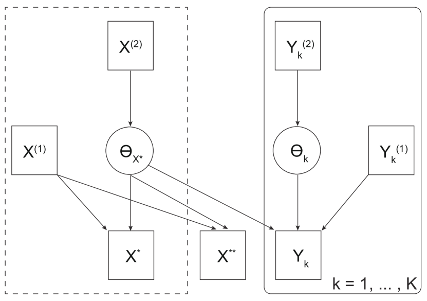
Figure 1: Self-contained Bayesian module. Squares denote observable random variables and circles denote parameters. The dashed part is a minimally self-contained Bayesian module (see Definition 2).

In practice, there is often a degree of choice about what data are used when inferring the parameter of interest $\Theta_{X^{\ast}}$ and so the posterior distribution (2) may not be the only potential distribution for $\Theta_{X^{\ast}}$. Specifically, there may be support variables $\Psi_{supp}$ that can be added to the existing variables $X^{\ast}$ and $X_{X^{\ast}}$ to form a model involving $\Theta_{X^{\ast}}$. Based on this consideration, we give the following definition:

Definition 2 (Self-contained Bayesian module for $X^{\ast}$).

Consider variables $\Psi=(X,\Theta)$ with joint distribution satisfying the Markov factorization property with respect to a DAG $G=(\Psi,E)$; observable random variables $X^{\ast}$, whose true generating process is of interest, with $X^{\ast}$-associated parameters $\Theta_{X^{\ast}}$ and $X^{\ast}$-associated observables $X_{X^{\ast}}$; and support variables $\Psi_{supp}=(X_{supp},\Theta_{supp})\subseteq\Psi\setminus(\Psi_{X^{\ast}}\cup X^{\ast})$. We say a set of variables $(X^{\ast},\Psi_{X^{\ast}},\Psi_{supp})$ form a self-contained Bayesian module for $X^{\ast}$ that can be used to estimate the true data generating process of $X^{\ast}$ if the posterior distribution given by

$$p(\Theta_{X^{\ast}}|X^{\ast},X_{X^{\ast}},X_{supp})=\int p(\Theta_{X^{\ast}},\Theta_{supp}|X^{\ast},X_{X^{\ast}},X_{supp})d\Theta_{supp}$$

is well defined given the DAG. When $\Psi_{supp}=\emptyset$, we say $(X^{\ast},\Psi_{X^{\ast}})$ forms a minimally self-contained Bayesian module for $X^{\ast}$.

To better understand Definition 2, consider the whole illustrative example in Figure 1 (not just that enclosed by a dashed line). In this case we have additional identically and independently distributed observables $X^{\ast\ast}$, as well as observables $\{Y_{k}\}_{k=1}^{K}$ associated with the $Y_{k}$-associated model $p(Y_{k}|\Theta_{k},\Theta_{X^{\ast}},Y_{k}^{(1)})$, which shares parameters in common with the model for $X^{\ast}$, and prior model $p(\Theta_{k}|Y_{k}^{(2)})$ for $k=1,\cdots,K$. The observables $\{Y_{k}\}_{k=1}^{K}$ and $X^{\ast\ast}$ provide information about the parameter of interest $\Theta_{X^{\ast}}$, so we call each

$$p(\Theta_{k},Y_{k}|\Theta_{X^{\ast}},Y_{k}^{(1)},Y_{k}^{(2)})=p(Y_{k}|\Theta_{k},\Theta_{X^{\ast}},Y_{k}^{(1)})p(\Theta_{k}|Y_{k}^{(2)}),\ \ k=1,\cdots,K;$$

and $p(X^{\ast\ast}|\Theta_{X^{\ast}},X^{(1)})$ support models. By combining all the $K+1$ support models with the $X^{\ast}$-associated model and prior model as shown in Figure 1, an alternative posterior distribution is given by

$$p(\Theta_{X^{\ast}}|X^{\ast},X_{X^{\ast}},X_{supp}) \propto p(X^{\ast}|\Theta_{X^{\ast}},X^{(1)})p(\Theta_{X^{\ast}}|X^{(2)})p(X^{\ast\ast}|\Theta_{X^{\ast}},X^{(1)})$$ (3)

$$\ \ \times\int\prod_{k=1}^{K}p(\Theta_{k},Y_{k}|\Theta_{X^{\ast}},Y_{k}^{(1)},Y_{k}^{(2)})d\Theta_{supp},$$

where $\Theta_{supp}=\cup_{k=1}^{K}\Theta_{k}$ and $X_{supp}=(X^{\ast\ast},\cup_{k=1}^{K}(Y_{k}\cup Y_{k}^{(1)}\cup Y_{k}^{(2)}))$.

Both (2) and (3) can be used to infer the parameter of interest $\Theta_{X^{\ast}}$ via a standard Bayesian framework and subsequently estimate the true data generating process of $X^{\ast}$. The difference is that (2) involves only the minimum information that is required to infer $\Theta_{X^{\ast}}$ whereas (3) involves additional information.

Self-contained Bayesian modules have two appealing properties. First, the module is defined with respect to a set of observable random variables $X^{\ast}$. Hence, the inference of the parameter $\Theta_{X^{\ast}}$ is meaningful in the sense that it can be always used to infer the data generating process of $X^{\ast}$. Second, clearly we can conduct standard Bayesian inference by only using information from the self-contained module. This makes it possible to prevent information from the outside of the module affecting inference because the module itself contains sufficient information to infer $\Theta_{X^{\ast}}$ within the Bayesian framework. This property will be helpful for modularized Bayesian inference.

2.3 Two-module case

Before we study the more general form of modularized Bayesian inference, we first consider spliting variables into two self-contained Bayesian modules. For this basic two-module case, we discuss how to identify the order between the two modules. We then propose and justify the cut distribution in this setting so that the inference of one module is not affected by the other.

2.3.1 Self-contained modules

We first group variables into two self-contained Bayesian modules (which may overlap). We defined a self-contained Bayesian module with respect to a set of observable random variables so, without loss of generality, we start by partitioning the observable random variables $X$ into two disjoint groups, which we call $X_{A}^{\ast}$ and $X_{B}^{\ast}$. Then we enlarge each set by incorporating variables until each forms a module that can be inferred without using information from the other module. In other words, each is a self-contained Bayesian module. This will form the basis of our framing of modularized Bayesian inference. We have the first rule.

Rule 1 (Identifying a self-contained module within a DAG).

Given a DAG $G=(\Psi,E)$ and a partition $X=X_{A}^{\ast}\cup X_{B}^{\ast}$, we form the set $\Psi_{A}=(X_{A},\Theta_{A})$ by augmenting the set of observable random variables $X_{A}^{\ast}$. For every directed path $b\rightsquigarrow a$ with $a=\psi_{1},\psi_{2},\cdots,\psi_{s}=b$ and the leaf $a\in X_{A}^{\ast}$, we consider the following two cases.

1. If there is a $\psi_{r}\in X_{B}^{\ast}$, $r>1$ such that $(\psi_{1},\cdots,\psi_{r-1})\notin X_{B}^{\ast}$, then we add $(\psi_{1},\psi_{2},\cdots,\psi_{r})$ into $\Psi_{A}$.

2. If directed path $b\rightsquigarrow a$ does not involve any node from $X_{B}^{\ast}$, then we add $(\psi_{1},\psi_{2},\cdots,\psi_{s})$ into $\Psi_{A}$.

We can form two modules $\Psi_{A}=(X_{A},\Theta_{A})$, which we call module A, and $\Psi_{B}=(X_{B},\Theta_{B})$, which we call module B, according to Rule 1. From now on, we interchangeably use module $I$ to refer set $\Psi_{I}$ and use $\Psi_{I}$ to refer module $I$, where $I$ is an arbitrary index. Note that there are also variables that belong to both modules or do not belong to any modules. Let $\Psi_{A\setminus B}$ denote the set of variables that belong to module $A$ but not module $B$ (with $\Psi_{B\setminus A}$ defined correspondingly); $\Psi_{A\cap B}$ denote the set of variables that belong to both modules; $\Psi_{A\cup B}$ denote the set of variables that either belong to modules $A$ or module $B$; and $\Psi_{(A\cup B)^{\mathsf{c}}}$ be the set of variables that do not belong to either module $A$ or $B$. We correspondingly define a partition of $X$ and $\Theta$. A Venn diagram illustrating the partition of $X$ is given in Figure 2.

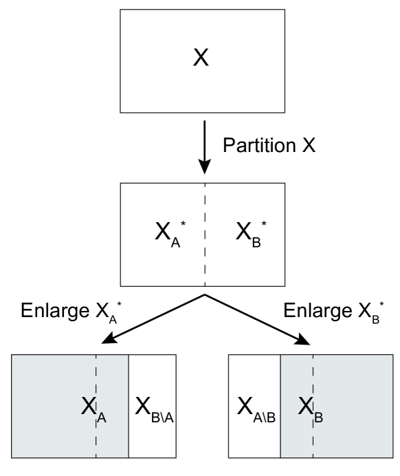
Figure 2: Partitioning the observable random variable $X$. First $X$ is partitioned into two disjoint group $X_{A}^{\ast}$ and $X_{B}^{\ast}$. Then $X_{A}^{\ast}$ is enlarged to form $\Psi_{A}=(X_{A},\Theta_{A})$ following Rule 1, and similarly for $X_{B}^{\ast}$ to form $\Psi_{B}=(X_{B},\Theta_{B})$. This leads to two overlapping sets $X_{A}$ and $X_{B}$.

Having partitioned the variables into four groups, we first study the topological structure of the DAG. To prevent information from the suspect module and facilitate deduction of the component of the cut distribution for parameters in the reliable module (we will later discuss this in Rule 3 in Section 2.3.2), we define a particular sub-graph of the DAG $G$:

Definition 3 ($\Psi_{0}$-cut-sub-graph).

Given a DAG $G=(\Psi,E)$ and a set of variables $\Psi_{0}\subseteq\Psi$, we define the cut-sub-graph $G_{\text{cut}(\Psi_{0})}=(\Psi,E_{0})$ in which edges from $\Psi\setminus\Psi_{0}$ to $\Psi_{0}$ are removed, i.e.,

$$E_{0}=\left\{a\rightarrow b\in E\ |\ (b\in\Psi\setminus\Psi_{0})\text{ or }(b\in\Psi_{0})\cap(a\in\Psi_{0})\right\}.$$

Now we have the following lemma for the topological structure of the DAG.

Lemma 1.

Given a DAG $G=(\Psi,E)$ and the partition $\Psi=\Psi_{A\setminus B}\,\cup\,\Psi_{B\setminus A}\,\cup\,\Psi_{A\cap B}\,\cup\,\Psi_{(A\cup B)^{\mathsf{c}}}$, then the following statements hold.

1. The set $\Psi_{(A\cup B)^{\mathsf{c}}}$ only contains parameters and there are no directed edges from $\Psi_{(A\cup B)^{\mathsf{c}}}$ to $\Psi_{A\cup B}$ (i.e., $\text{ch}(\Psi_{(A\cup B)^{\mathsf{c}}})=\emptyset$).

2. The set of parent nodes $\text{pa}(\Psi_{A\setminus B})$ of set $\Psi_{A\setminus B}$ are in $\Psi_{A\cap B}$. The set of child nodes $\text{ch}(\Psi_{A\setminus B})$ of set $\Psi_{A\setminus B}$ are in $\Psi_{A\cap B}\cup\Psi_{(A\cup B)^{\mathsf{c}}}$. The equivalent results hold for $\Psi_{B\setminus A}$.

3. Given variables $\psi_{A\cap B}\in\Psi_{A\cap B}$, $\psi_{A\setminus B}\in\Psi_{A\setminus B}$ and $\psi_{B\setminus A}\in\Psi_{B\setminus A}$, a V-structure $\psi_{A\setminus B}\rightarrow\psi_{A\cap B}\leftarrow\psi_{B\setminus A}$ does not exist.

4. The set of parent nodes $\text{pa}(\Theta_{A\cap B})$ of set $\Theta_{A\cap B}$ are in $X_{A\cap B}$ and the set of parent nodes $\text{pa}(X_{A\cap B})$ of set $X_{A\cap B}$ are in $\{\Theta_{A\cap B},\Theta_{A\setminus B},\Theta_{B\setminus A},X_{A\setminus B},X_{B\setminus A}\}$.

5. $\Psi_{A\cap B}=\emptyset$ if and only if there is no path between $\Psi_{A}$ and $\Psi_{B}$ in the $\Psi_{(A\cup B)^{\mathsf{c}}}$-cut-sub-graph $G_{\text{cut}(\Psi_{(A\cup B)^{\mathsf{c}}})}$ (i.e., $G_{\text{cut}(\Psi_{(A\cup B)^{\mathsf{c}}})}$ has two disconnected components which are formed separately by nodes $\Psi_{A}$ and $\Psi_{B}$).

Proof.

The proof is in the appendix.

Having Lemma 1, we have the following lemma.

Lemma 2.

$\Psi_{A\setminus B}$ and $\Psi_{B\setminus A}$ are d-separated by $\Psi_{A\cap B}$ in DAG $G$ and we have

$$\Psi_{A\setminus B}\raisebox{0.45003pt}{\rotatebox[origin={c}]{90.0}{$\models$}}\Psi_{B\setminus A}|\Psi_{A\cap B}.$$

Proof.

The proof is in the appendix.

Now we consider whether we can infer each module without using the other module. This is equivalent to requiring both modules to be self-contained Bayesian modules. We have the following theorem:

Theorem 1.

Rule 1 builds two minimally self-contained Bayesian modules $\Psi_{A}$ and $\Psi_{B}$ because their posterior distributions can be built as:

$$p(\Theta_{A}|X_{A})\propto p(\Theta_{A\setminus B}|\text{pa}(\Theta_{A\setminus B}))p(\Theta_{A\cap B}|\text{pa}(\Theta_{A\cap B}))p(X_{A\setminus B}|\text{pa}(X_{A\setminus B}))$$

$$\ \ \times p(X_{A\cap B}\cap X_{A}^{\ast}|\text{pa}(X_{A\cap B}\cap X_{A}^{\ast}));$$

$$p(\Theta_{B}|X_{B})\propto p(\Theta_{B\setminus A}|\text{pa}(\Theta_{B\setminus A}))p(\Theta_{A\cap B}|\text{pa}(\Theta_{A\cap B}))p(X_{B\setminus A}|\text{pa}(X_{B\setminus A}))$$

$$\ \ \times p(X_{A\cap B}\cap X_{B}^{\ast}|\text{pa}(X_{A\cap B}\cap X_{B}^{\ast})).$$

Proof.

The proof is in the appendix.

2.3.2 Inference: standard and cut distributions

We first consider the distribution of $\Theta$ given $X$ obtained using standard Bayesian inference. Note that the complete variable set $\Psi$ is naturally a self-contained Bayesian module.

Lemma 3.

Given two modules $A$ and $B$, the standard posterior distribution for $\Theta$ can be written as either

$$p(\Theta|X)=p(\Theta_{(A\cup B)^{\mathsf{c}}}|\text{pa}(\Theta_{(A\cup B)^{\mathsf{c}}}))p(\Theta_{B\setminus A}|\Theta_{A\cap B},X_{B\setminus A},X_{A\cap B})p(\Theta_{A}|X)$$

or

$$p(\Theta|X)=p(\Theta_{(A\cup B)^{\mathsf{c}}}|\text{pa}(\Theta_{(A\cup B)^{\mathsf{c}}}))p(\Theta_{A\setminus B}|\Theta_{A\cap B},X_{A\setminus B},X_{A\cap B})p(\Theta_{B}|X).$$

Proof.

The proof is in the appendix.

The standard posterior distribution tells us that the inference of one module might be affected by the other module under the standard Bayesian framework.

To obtain the cut distribution for $\Theta$, we need to identify the relationship between the modules. We can then decide the module whose influence to the other module needs to be “cut”. We have the following second rule:

Rule 2 (Identifying the order within a two-module case).

Given the DAG $G=(\Psi,E)$, if there is a directed edge $\psi_{1}\rightarrow\psi_{2}$, where $\psi_{1}\in\Psi_{A\cap B}$ and $\psi_{2}\in\Psi_{B\setminus A}$, then we denote this as $A\rightharpoonup B$ (or $B\leftharpoonup A$). If we have $A\rightharpoonup B$ but not $B\rightharpoonup A$, then module $A$ is the parent module and $B$ is its child module. If both $A\rightharpoonup B$ and $B\rightharpoonup A$ are true, an order must be chosen by the user of the model. If neither $A\rightharpoonup B$ nor $B\rightharpoonup A$, we say that two modules are unordered and denoted as $(A,B)$.

Rule 2 clarifies the order between module $A$ and $B$. When only one type of order is true (i.e., either $A\rightharpoonup B$ or $B\rightharpoonup A$), then this order is fixed. When both $A\rightharpoonup B$ and $B\rightharpoonup A$ are true, selecting the order is a choice for the user. We normally set the more suspect module to be the child module, which will prevent it from affecting inference for the parent module. By the fifth statement of Lemma 1, the fact that two modules are unordered indicates $\Psi_{A\cap B}=\emptyset$. Hence by Lemma 2, they are independent and inference is completely separate.

Now we consider cutting the influence from one module. Theorem 1 ensures that we can infer one module without being affected by the other module, although inference is determined by variables that are shared with the other module (i.e., $X_{A\cap B}\cap X_{B}^{\ast}$). Therefore, a viable choice of distribution for $\Theta$ given $X$ involves $p(\Theta_{A}|X_{A})$, instead of the $p(\Theta_{A}|X)$ in the standard posterior distribution as shown in Lemma 3. This is described in the following rule.

Rule 3 (Cutting the feedback).

To cut the feedback from child module $B$ to parent module $A$, we prune the original DAG $G$ to obtain the $\Psi_{(B\setminus A)\cup(A\cup B)^{\mathsf{c}}}$-cut-sub-graph $G_{\text{cut}(\Psi_{(B\setminus A)\cup(A\cup B)^{\mathsf{c}}})}$. The component of the cut distribution for parameters $\Theta_{A}$ is the posterior distribution of $\Theta_{A}$ in $G_{\text{cut}(\Psi_{(B\setminus A)\cup(A\cup B)^{\mathsf{c}}})}$. Note that under $G_{\text{cut}(\Psi_{(B\setminus A)\cup(A\cup B)^{\mathsf{c}}})}$, this posterior distribution is $p(\Theta_{A}|X_{A})$.

Rule 3 tells us how to infer the parent module A. The remaining part that we have not inferred is $\Psi_{B\setminus A}$ of module $B$. Note that, although module $B$ is self-contained, the parameters $\Theta_{A\cap B}$ that are in module B but also in module A have now been inferred according to Rule 3. Therefore, standard Bayesian inference cannot be immediately used within module $B$. We introduce the following definition.

Definition 4 (Conditional self-contained Bayesian inference).

Consider a DAG $G=(\Psi,E)$ with two minimally self-contained Bayesian modules $\Psi_{A}=(X_{A},\Theta_{A})$ and $\Psi_{B}=(X_{B},\Theta_{B})$. Suppose that we choose to estimate a set of parameters $\Theta_{fix}\subseteq\Theta_{B}$ using only module A or using only its own prior distribution $p(\Theta_{fix}|\text{pa}(\Theta_{fix}))$. Then we say conditional self-contained Bayesian inference for $\Theta_{unfix}=\Theta_{B}\setminus\Theta_{fix}$ is conducted when the posterior distribution is given by

$$p(\Theta_{unfix}|\Theta_{fix},X_{B})$$

where for any $\theta^{\ast}\in\Theta_{fix}$ we have either

$$\theta^{\ast}\sim p(\theta^{\ast}|\text{pa}(\theta^{\ast}))$$

or

$$\theta^{\ast}\sim\int p(\Theta_{A}|X_{A})\ d(\Theta_{A}\setminus\theta^{\ast}).$$

The aim of self-contained Bayesian modules is to prevent using information that is external to the module, whereas the aim of conditional self-contained Bayesian inference is to prevent using (at least some) information that is internal to a module. More specifically, it prevents inference for some parameters being affected by observable random variables within the same module.

We now return to the question of inference for module B under the two-module case when part of its parameters $\Theta_{A\cap B}$ have been inferred by its parent module $A$. To infer the remaining component $\Theta_{B\setminus A}$ we propose to conduct the conditional self-contained Bayesian inference. This let us build the final piece of the cut distribution. We have the following rule:

Rule 4 (Formulating the cut distribution).

When the modules’ order is $A\rightharpoonup B$, the cut distribution for parameters $\Theta$ is:

$$p_{A\rightharpoonup B}(\Theta|X):=p(\Theta_{(A\cup B)^{\mathsf{c}}}|\text{pa}(\Theta_{(A\cup B)^{\mathsf{c}}}))p(\Theta_{B\setminus A}|\Theta_{A\cap B},X_{B\setminus A},X_{A\cap B})p(\Theta_{A}|X_{A}).$$

Similarly, when the modules’ order is $B\rightharpoonup A$, the cut distribution is

$$p_{B\rightharpoonup A}(\Theta|X):=p(\Theta_{(A\cup B)^{\mathsf{c}}}|\text{pa}(\Theta_{(A\cup B)^{\mathsf{c}}}))p(\Theta_{A\setminus B}|\Theta_{A\cap B},X_{A\setminus B},X_{A\cap B})p(\Theta_{B}|X_{B}).$$

When two modules are unordered, the cut distribution is

$$p_{(A,B)}(\Theta|X):=p(\Theta_{(A\cup B)^{\mathsf{c}}}|\text{pa}(\Theta_{(A\cup B)^{\mathsf{c}}}))p(\Theta_{B}|X_{B})p(\Theta_{A}|X_{A}).$$

It is easy to check that both $p_{A\rightharpoonup B}$ and $p_{B\rightharpoonup A}$ are valid probability distributions but they might be different from either each other or the standard posterior distribution. When the order of module is $A\rightharpoonup B$, the inference of parameters $\Theta_{A}$ is solely determined by the observable random variables $X_{A}$ from the same module. This is in contrast to standard Bayesian inference or inference when assuming $B\rightharpoonup A$, in which inference of $\Theta_{A}$ might be influenced by variables in module $B$. Note that, the distribution of $\Theta_{(A\cup B)^{\mathsf{c}}}$ conditional on its parents $\text{pa}(\Theta_{(A\cup B)^{\mathsf{c}}})$ is unchanged no matter what kind of inference model we use and there is no feedback from $\Psi_{(A\cup B)^{\mathsf{c}}}$. In addition, $p_{(A,B)}(\Theta|X)=p(\Theta|X)$ when $\Psi_{A\cap B}=\emptyset$ (i.e., $A$ and $B$ are unordered). Hence, we conclude that cut distribution $p_{A\rightharpoonup B}$ prevents information from variables $\Psi_{B\setminus A}$.

2.3.3 Theoretical properties

We now justify the cut distribution. In the case of $A\rightharpoonup B$, we know that $p(\Theta_{(A\cup B)^{\mathsf{c}}}|\text{pa}(\Theta_{(A\cup B)^{\mathsf{c}}}))$ is unchanged in standard posterior distribution and cut distribution. The component $p(\Theta_{A}|X_{A})$ is justified by Theorem 1. The only component that we need to justify is $p(\Theta_{B\setminus A}|\Theta_{A\cap B},X_{B\setminus A},X_{A\cap B})$. Given arbitrary two distributions $f_{1}(x)$ and $f_{2}(x)$, define the Kullback-Leibler (KL) divergence between $f_{1}(x)$ and $f_{2}(x)$ as:

$$\mathbb{D}_{KL}(f_{1}(\cdot),f_{2}(\cdot)):=\int f_{1}(x)\log(f_{1}(x)/f_{2}(x))dx.$$

We have the following theorem:

Theorem 2.

Let $f(\Theta_{B\setminus A})$ be a probability density function for parameters $\Theta_{B\setminus A}$. Given the joint distribution $p(X,\Theta)$ and denote:

$$p_{f}(\Theta)=p(\Theta_{(A\cup B)^{\mathsf{c}}}|\text{pa}(\Theta_{(A\cup B)^{\mathsf{c}}}))f(\Theta_{B\setminus A})p(\Theta_{A}|X_{A}),$$

we have

$$p(\Theta_{B\setminus A}|\Theta_{A\cap B},X_{B\setminus A},X_{A\cap B})\propto\operatorname*{arg\,min}_{f(\Theta_{B\setminus A})}\mathbb{D}_{KL}\left(p_{f}(\cdot),p(X,\cdot)\right).$$

Proof.

The proof is in the appendix.

2.4 Within-module cut

We now consider the case when we regard some prior knowledge as more reliable than the information from the observations for some specific parameters, but inference for other parameters still depends on the observations. To do this requires within-module manipulation and, given Definition 4, a specific type of conditional self-contained Bayesian inference. The within-module cut aims to protect the inference of some parameters from being affected by the suspect information from observations.

As an example, consider the self-contained module depicted in Figure 1 and Figure 3(a). The parameter of interest is $\Theta_{X^{\ast}}$ and its posterior is equation (2). Clearly, posterior (2) is affected by the observable variable $X^{\ast}$. An alternative distribution for $\Theta_{X^{\ast}}$ is simply its prior distribution $p(\Theta_{X^{\ast}}|X^{(2)})$. Using this prior alone means that we do not include any information from the associated observable variable $X^{\ast}$.

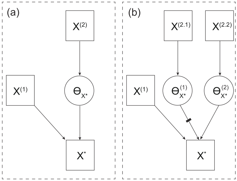
Figure 3: Within-module manipulation. Panel (b) is a model based on panel (a) where $\Theta_{X^{\ast}}=(\Theta_{X^{\ast}}^{(1)},\Theta_{X^{\ast}}^{(2)})$ and $X^{(2)}=(X^{(2.1)},X^{(2.2)})$. In panel (b), parameter $\Theta_{X^{\ast}}^{(1)}$ is inferred solely by its prior.

A more involved case occurs when we split parameters of interest $\Theta_{X^{\ast}}$ into two parts $(\Theta_{X^{\ast}}^{(1)},\Theta_{X^{\ast}}^{(2)})$, as in Figure 3(b), and seek to use only the prior for $\Theta_{X^{\ast}}^{(1)}$ but infer the other part $\Theta_{X^{\ast}}^{(2)}$ by conditioning on $\Theta_{X^{\ast}}^{(1)}$. That is:

$$p(\Theta_{X^{\ast}}^{(1)},\Theta_{X^{\ast}}^{(2)})=p(\Theta_{X^{\ast}}^{(2)}|\Theta_{X^{\ast}}^{(1)},X^{\ast},X^{(2.2)})p(\Theta_{X^{\ast}}^{(1)}|X^{(2.1)}),$$ (4)

where

$$p(\Theta_{X^{\ast}}^{(2)}|\Theta_{X^{\ast}}^{(1)},X^{\ast},X^{(2.2)})\propto p(X^{\ast}|\Theta_{X^{\ast}}^{(1)},\Theta_{X^{\ast}}^{(2)},X^{(1)})p(\Theta_{X^{\ast}}^{(2)}|X^{(2.2)}).$$

Unlike the posterior distribution and prior distribution, (4) applies a within-module cut such that the inference of $\Theta_{X^{\ast}}^{(1)}$ does not depend on its associated observable variable $X^{\ast}$. Note that clearly (4) is a proper probability distribution.

2.5 Three-module case

Consider now the case of three modules, in which the observable random variable $X$ can be partitioned into three disjoint groups. We will obtain a split into three modules by splitting either the child module or the parent module from a two module split; this will form the basis for a more generalized multiple-module case in Section 2.6. In this section, we discuss the methodology of splitting two modules into three, and cut inference within this three-module framework.

To obtain three modules, we first split the variables into two modules, denoted here as $A$ and $T$. Recall that some variables may belong to $(A\cup T)^{\mathsf{c}}$. By Rule 2 we can determine the order between $A$ and $T$. We then obtain the third module by splitting module $T$. Module $T$ originates from observable random variables $X_{T}^{\ast}$, so we split this set into two disjoint groups $X_{B}^{\ast}$ and $X_{C}^{\ast}$. We can then identify module $B$ by applying Rule 1 with the exception that we replace the “$X_{B}^{\ast}$” in Rule 1 by $X_{A}^{\ast}\cup X_{C}^{\ast}$; and correspondingly for module $C$. In this way we obtain three modules $A$, $B$ and $C$, where $\Psi_{B}\cup\Psi_{C}=\Psi_{T}$.

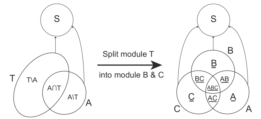
Figure 4: Splitting module $T$ into modules $B$ and $C$. An arrow represents all directed edges from modules to $S=(A\cup T)^{\mathsf{c}}$.

We now need to identify the ordering of modules $B$ and $C$. To simplify the exposition, we use the following notation to denote various sets:

$$\underline{A}=A\setminus\left(B\cup C\right);\ \underline{B}=B\setminus\left(A\cup C\right);\ \underline{C}=C\setminus\left(A\cup B\right);$$

$$\underline{\underline{A}}=A\setminus\underline{A};\ \underline{\underline{B}}=B\setminus\underline{B};\ \underline{\underline{C}}=C\setminus\underline{C};$$

$$\underline{AB}=\left(A\cap B\right)\setminus C;\ \underline{AC}=\left(A\cap C\right)\setminus B;\ \underline{BC}=\left(B\cap C\right)\setminus A;$$

$$\underline{ABC}=\left(A\cap B\cap C\right);$$

We partition the variables $\Psi_{A\cup B\cup C}$ into 7 disjoint groups: $\Psi_{\underline{A}}$, $\Psi_{\underline{AB}}$, $\Psi_{\underline{AC}}$, $\Psi_{\underline{ABC}}$, $\Psi_{\underline{B}}$, $\Psi_{\underline{BC}}$ and $\Psi_{\underline{C}}$, as shown in Figure 4. For notational simplicity we define $\Psi_{S}:=\Psi_{(A\cup B)^{\mathsf{c}}}$, which remains unchanged. Since module $A$ is the parent module of module $T=B\cup C$, the parameters $\Theta_{A}$ can be inferred separately from $\Psi_{T\setminus A}$ by Theorem 1. We have the following lemma:

Lemma 4.

If $\Psi_{\underline{BC}}\neq\emptyset$, then there must be at least one edge $a\rightarrow b$ where $a\in\Psi_{\underline{BC}}$ and $b\in(\Psi_{\underline{B}}\cup X_{B}^{\ast})\cup(\Psi_{\underline{C}}\cup X_{C}^{\ast})$. Otherwise if $\Psi_{\underline{BC}}=\emptyset$, we have

$$\Psi_{\underline{B}}\raisebox{0.45003pt}{\rotatebox[origin={c}]{90.0}{$\models$}}\Psi_{\underline{C}}|\Psi_{A}.$$

Proof.

The proof is in the appendix.

Given Lemma 4, we give the following definition:

Rule 5 (Identifying the order within a three-module case).

We consider it in three scenarios:

1. The order before splitting is $A\rightharpoonup(B\cup C)$ (i.e., we split the child module). This means that at least one of $\Psi_{A\cap B}$ and $\Psi_{A\cap C}$ must be non-empty.

   1. When both $\Psi_{A\cap B}\neq\emptyset$ and $\Psi_{A\cap C}\neq\emptyset$.

      1. If there is at least one edge $b\rightarrow c$ where $b\in\Psi_{\underline{BC}}$ and $c\in(\Psi_{\underline{C}}\cup X_{C}^{\ast})$, we say module $C$ is the child module of module $B$ and module $B$ is the child module of module $A$ and we can denote it as $A\rightharpoonup B\rightharpoonup C$. Similarly we can denote $A\rightharpoonup C\rightharpoonup B$ if there is at least one edge $c\rightarrow b$ where $c\in\Psi_{\underline{BC}}$ and $b\in(\Psi_{\underline{B}}\cup X_{B}^{\ast})$.

      2. If $\Psi_{\underline{BC}}=\emptyset$, we say module $B$ and $C$ are unordered and they are child modules of module $A$ and denote it as $A\rightharpoonup(B,C)$.

   2. When only $\Psi_{A\cap B}$ or $\Psi_{A\cap C}$ is not empty. Without loss of generality, we consider only $\Psi_{A\cap C}=\emptyset$ here.

      1. If there is at least one edge $b\rightarrow c$ where $b\in\Psi_{\underline{BC}}$ and $c\in(\Psi_{\underline{C}}\cup X_{C}^{\ast})$, we say module $C$ is the child module of module $B$ and module $B$ is the child module of module $A$ and we can denote it as $A\rightharpoonup B\rightharpoonup C$.

      2. If there is at least one edge $c\rightarrow b$ where $c\in\Psi_{\underline{BC}}$ and $b\in(\Psi_{\underline{B}}\cup X_{B}^{\ast})$, we say module $A$ and $C$ are unordered and they are parent modules of module $B$ and can denote it as $(A,C)\rightharpoonup B$.

      3. If $\Psi_{\underline{BC}}=\emptyset$, we say module $B$ is the child module of module $A$ and they are unordered with module $C$ and can denote it as $(C,(A\rightharpoonup B))$.

2. The order before splitting is $(B\cup C)\rightharpoonup A$ (i.e., we split the parent module). This means that at least one of $\Psi_{A\cap B}$ and $\Psi_{A\cap C}$ must be non-empty.

   1. When both $\Psi_{A\cap B}\neq\emptyset$ and $\Psi_{A\cap C}\neq\emptyset$.

      1. If there is at least one edge $b\rightarrow c$ where $b\in\Psi_{\underline{BC}}$ and $c\in(\Psi_{\underline{C}}\cup X_{C}^{\ast})$, we say module $C$ is the child module of module $B$ and module $A$ is the child module of module $C$ and we can denote it as $B\rightharpoonup C\rightharpoonup A$. Similarly we can denote $C\rightharpoonup B\rightharpoonup A$ if there is at least one edge $c\rightarrow b$ where $c\in\Psi_{\underline{BC}}$ and $b\in(\Psi_{\underline{B}}\cup X_{B}^{\ast})$.

      2. If $\Psi_{\underline{BC}}=\emptyset$, we say module $B$ and $C$ are unordered and they are parent modules of module $A$ and can denote it as $(B,C)\rightharpoonup A$.

   2. When only $\Psi_{A\cap B}$ or $\Psi_{A\cap C}$ is not empty. Without loss of generality, we consider only $\Psi_{A\cap C}=\emptyset$ here.

      1. If there is at least one edge $b\rightarrow c$ where $b\in\Psi_{\underline{BC}}$ and $c\in(\Psi_{\underline{C}}\cup X_{C}^{\ast})$, we say module $A$ and module $C$ are unordered and they are child modules of module $B$ and we can denote it as $B\rightharpoonup(A,C)$.

      2. If there is at least one edge $c\rightarrow b$ where $c\in\Psi_{\underline{BC}}$ and $b\in(\Psi_{\underline{B}}\cup X_{B}^{\ast})$, we say module $A$ is the child module of module $B$ and module $B$ is the child module of module $C$ and can denote it as $C\rightharpoonup B\rightharpoonup A$.

      3. If $\Psi_{\underline{BC}}=\emptyset$, we say module $A$ is the child module of module $B$ and they are unordered with module $C$ and can denote it as $(C,(B\rightharpoonup A))$.

3. The order before splitting is $(A,(B\cup C))$ (i.e., module $A$ and $B\cup C$ are unordered. This means that both $\Psi_{A\cap B}$ and $\Psi_{A\cap C}$ must be empty.

   1. If there is at least one edge $b\rightarrow c$ where $b\in\Psi_{\underline{BC}}$ and $c\in(\Psi_{\underline{C}}\cup X_{C}^{\ast})$, we say module $C$ is the child module of module $B$ and they are unordered with module $A$ and denote it as $(A,(B\rightharpoonup C))$. Similarly we can denote $(A,(C\rightharpoonup B))$ if there is at least one edge $c\rightarrow b$ where $c\in\Psi_{\underline{BC}}$ and $b\in(\Psi_{\underline{B}}\cup X_{B}^{\ast})$.

   2. If $\Psi_{\underline{BC}}=\emptyset$, we say module $A$, $B$ and $C$ are unordered and denote it as $(A,B,C)$.

Having defined the order within a three-module case, we can draw a ordering plot for a clear illustration of the relationship between modules. In an ordering plot, we use a circle to denote a module and a module $A$ is a parent module of another module $B$ if and only if there is an arrow originated from $A$ to $B$. Some typical examples of ordering plot when splitting a two-module case to a three-module case are shown in Figure 5.

Figure 5: Ordering plot of different types of orders among three modules result from a split of two modules. A circle represents a module and an arrow represents a direction of ordering between modules. (a). Depicts the possible ordering of three modules when splitting module $T$ when the original order is $A\rightharpoonup T$: $(A,B)\rightharpoonup C$; $A\rightharpoonup B\rightharpoonup C$; $A\rightharpoonup(B,C)$ and $(C,(A\rightharpoonup B))$ (from top to bottom). (b). Orders among tree modules when splitting module $T$ and the original two modules are unordered: $(A,(B\rightharpoonup C))$ and $(A,B,C)$ (from top to bottom).

Now we can derive the cut distribution for the three-module case in a similar manner to the two-module case. We have the following definition:

Definition 5 (Splitting the cut distribution).

The cut distribution for the three-module case is:

1. When $A\rightharpoonup B\rightharpoonup C$,

   $$p_{A\rightharpoonup B\rightharpoonup C}(\Theta|X)$$

   $$\ :=p(\Theta_{S}|\Theta_{A\cup B\cup C},X)p(\Theta_{\underline{C}}|\Theta_{\underline{\underline{C}}},X_{C})p(\Theta_{B\setminus A}|\Theta_{A\cap B},X_{B})p(\Theta_{A}|X_{A}).$$

2. When $A\rightharpoonup C\rightharpoonup B$,

   $$p_{A\rightharpoonup C\rightharpoonup B}(\Theta|X)$$

   $$\ :=p(\Theta_{S}|\Theta_{A\cup B\cup C},X)p(\Theta_{\underline{B}}|\Theta_{\underline{\underline{B}}},X_{B})p(\Theta_{C\setminus A}|\Theta_{A\cap C},X_{C})p(\Theta_{A}|X_{A}).$$

3. When modules $B$ and $C$ are unordered and they are child modules of modules $A$,

   $$p_{A\rightharpoonup(B,C)}(\Theta|X)$$

   $$\ :=p(\Theta_{S}|\Theta_{A\cup B\cup C},X)p(\Theta_{\underline{C}}|\Theta_{A\cap C},X_{C})p(\Theta_{\underline{B}}|\Theta_{A\cap B},X_{B})p(\Theta_{A}|X_{A}).$$

4. When modules $A$ and $B$ are unordered and they are parent modules of module $C$,

   $$p_{(A,B)\rightharpoonup C}(\Theta|X):=p(\Theta_{S}|\Theta_{A\cup B\cup C},X)p(\Theta_{\underline{C}}|\Theta_{\underline{\underline{C}}},X_{C})p(\Theta_{B}|X_{B})p(\Theta_{A}|X_{A}).$$

5. When module $C$ is the child module of module $B$ and they are unordered with module $A$,

   $$p_{(A,(B\rightharpoonup C))}(\Theta|X):=p(\Theta_{S}|\Theta_{A\cup B\cup C},X)p(\Theta_{\underline{C}}|\Theta_{B\cap C},X_{C})p(\Theta_{B}|X_{B})p(\Theta_{A}|X_{A}).$$

6. When module $A$, $B$ and $C$ are unordered,

   $$p_{(A,B,C)}(\Theta|X):=p(\Theta_{S}|\Theta_{A\cup B\cup C},X)p(\Theta_{C}|X_{C})p(\Theta_{B}|X_{B})p(\Theta_{A}|X_{A}).$$

Importantly, Definition 5 indicates that, when splitting a two-module case to a three-module case, the component of the cut distribution for the module that is not split remains unchanged. This important property enables us to only modify components of a cut distribution that involve modules being split while keeping the other components of the cut distribution unchanged.

We discuss the construction of the cut distribution by using $A\rightharpoonup B\rightharpoonup C$ as an example. As in the two-module case, $p(\Theta_{S}|\text{pa}(\Theta_{S}))=p(\Theta_{S}|\Theta_{A\cup B\cup C},X)$ is directly borrowed from the joint distribution (1) to form the component of the cut distribution for $\Theta_{S}$. Next, the procedure is the same as Rule 3, except that conditional self-contained Bayesian inferences are conducted for module $B$ (conditional on everything that has been inferred in module $A$) and $C$ (conditional on everything that has been inferred in module $A$ and $B$). If we regard module $B$ and $C$ as a single module, then by Rule 3 we can write the component of the cut distribution for parameters $\theta\in\Theta_{A}$: $p(\Theta_{A}|X_{A})$, which is exactly the same as the component of the cut distribution in the two-module case (see Theorem 1). That is:

$$p(\Theta_{A}|X_{A})\propto p(\Theta_{A}|\text{pa}(\Theta_{A}))p(X_{\underline{A}}|\text{pa}(X_{\underline{A}}))p(X_{A\cap(B\cup C)}\cap X_{A}^{\ast}|\text{pa}(X_{A\cap(B\cup C)}\cap X_{A}^{\ast})).$$

The next set of parameters of interest involves parameters in module $B$ that are not in module A. These are $\Theta_{\underline{B}}$ and $\Theta_{\underline{BC}}$, since $\Theta_{B\setminus A}=\Theta_{\underline{B}}\cup\Theta_{\underline{BC}}$. Conditional on information from module $A$, in order to prevent information from module $C$, we conduct conditional self-contained Bayesian inference for module $B$ by utilizing the following components of the joint distribution (1), which involve the distribution of $\Theta_{B\setminus A}$ and distributions conditioning on any variables from $\Theta_{B\setminus A}$ but neither conditioning on nor involving any variables from $\Psi_{\underline{C}}$, to form the component of the cut distribution of $\Theta_{B\setminus A}$:

$$p(\Theta_{B\setminus A}|\Theta_{A},X_{A\cup B})$$

$$\propto p(\Theta_{\underline{B}}|\text{pa}(\Theta_{\underline{B}}))p(\Theta_{\underline{BC}}|\text{pa}(\Theta_{\underline{BC}}))p(X_{\underline{B}}|\text{pa}(X_{\underline{B}}))p(X_{\underline{AB}}\cap X_{B}^{\ast}|\text{pa}(X_{\underline{AB}}\cap X_{B}^{\ast}))$$

$$\ \ \times p(X_{\underline{BC}}\cap X_{B}^{\ast}|\text{pa}(X_{\underline{BC}}\cap X_{B}^{\ast}))p(X_{\underline{ABC}}\cap X_{B}^{\ast}|\text{pa}(X_{\underline{ABC}}\cap X_{B}^{\ast})),$$

where the proportionality holds here because $\Theta_{A}$ has been inferred in module $A$. In addition, we have

$$\text{pa}(\Theta_{\underline{B}})\subseteq\left\{\Theta_{\underline{\underline{B}}},X_{B}\right\};\ \text{pa}(\Theta_{\underline{BC}})\subseteq\left\{\Theta_{\underline{ABC}},X_{B\cap C}\right\};\ \text{pa}(X_{\underline{B}})\subseteq\left\{\Theta_{B},X_{\underline{\underline{B}}}\right\};$$

$$\text{pa}(X_{\underline{AB}}\cap X_{B}^{\ast})\subseteq\{\Theta_{B},X_{B}\setminus X_{\underline{AB}},X_{\underline{AB}}\cap X_{A}^{\ast}\};$$

$$\text{pa}(X_{\underline{BC}}\cap X_{B}^{\ast})\subseteq\{\Theta_{B},X_{B}\setminus X_{\underline{BC}},X_{\underline{BC}}\cap X_{C}^{\ast}\};$$

$$\text{pa}(X_{\underline{ABC}}\cap X_{B}^{\ast})\subseteq\left\{\Theta_{B},X_{B}\setminus X_{\underline{ABC}},X_{\underline{ABC}}\cap(X_{A}^{\ast}\cup X_{C}^{\ast})\right\},$$

where all parameters involved in these set of parent nodes belong to $\Theta_{B}=\Theta_{B\setminus A}\cup\Theta_{A\cap B}$ and $\Theta_{A\cap B}$ has been inferred in module $A$. Hence we can write $p(\Theta_{B\setminus A}|\Theta_{A},X_{A\cup B})=p(\Theta_{B\setminus A}|\Theta_{A\cap B},X_{B})$. Now we conduct conditional self-contained Bayesian inference for module $C$ by utilizing all remaining components of the joint distribution (1) to form the final piece of component of the cut distribution for $\Theta_{\underline{C}}$:

$$p(\Theta_{\underline{C}}|\Theta_{A\cup B},X)$$

$$\propto p(\Theta_{\underline{C}}|\text{pa}(\Theta_{\underline{C}}))p(X_{\underline{C}}|\text{pa}(X_{\underline{C}}))p(X_{\underline{BC}}\cap X_{C}^{\ast}|\text{pa}(X_{\underline{BC}}\cap X_{C}^{\ast}))$$

$$\ \ \times p(X_{\underline{AC}}\cap X_{C}^{\ast}|\text{pa}(X_{\underline{AC}}\cap X_{C}^{\ast}))p(X_{\underline{ABC}}\cap X_{C}^{\ast}|\text{pa}(X_{\underline{ABC}}\cap X_{C}^{\ast})),$$

where we similarly have

$$\text{pa}(\Theta_{\underline{C}})\subseteq\left\{\Theta_{\underline{\underline{C}}},X_{C}\right\};\ \text{pa}(X_{\underline{C}})\subseteq\left\{\Theta_{C},X_{\underline{\underline{C}}}\right\};$$

$$\text{pa}(X_{\underline{BC}}\cap X_{C}^{\ast})\subseteq\{\Theta_{C},X_{C}\setminus X_{\underline{BC}},X_{\underline{BC}}\cap X_{B}^{\ast}\};$$

$$\text{pa}(X_{\underline{AC}}\cap X_{C}^{\ast})\subseteq\{\Theta_{C},X_{C}\setminus X_{\underline{AC}},X_{\underline{AC}}\cap X_{A}^{\ast}\};$$

$$\text{pa}(X_{\underline{ABC}}\cap X_{C}^{\ast})\subseteq\left\{\Theta_{C},X_{C}\setminus X_{\underline{ABC}},X_{\underline{ABC}}\cap(X_{A}^{\ast}\cup X_{B}^{\ast})\right\}.$$

Hence, we conclude that $p(\Theta_{\underline{C}}|\Theta_{A\cup B},X)=p(\Theta_{\underline{C}}|\Theta_{\underline{\underline{C}}},X_{C})$.

In summary, the essential procedure is to split the observable random variables into three disjoint groups and enlarge these groups according to Rule 1, then determine the internal order between the modules. The cut distribution of a three-module case is then formed by four components: three components for inferences of three modules and one component for the inference of $\Theta_{S}$. All possibilities of the cut distribution of a three-module case have been covered by Definition 5.

2.6 Multiple-module case: Sequential splitting technique

Now we have discussed the case when we split two modules into three modules, we can derive a further extension to continue splitting modules sequentially. This enables us to construct a general modularized framework.

We consider splitting an arbitrary module. The key is to reduce this complex structure of modules into the simple structure that we have discussed before. Here we mainly consider the case when this module has both parent modules and child modules. The case when it only has parent modules or child modules can be easily extended. We give the following definition:

Definition 6 (Ancestor and descendant module).

Given an arbitrary module $T$ and an ordering plot $J$ that contains module $T$:

1. If there is a direct path $A\rightsquigarrow T$ between two modules $A$ and $T$ with a path $A=M_{1},M_{2},\cdots,M_{s}=T$ in the ordering plot $J$, then module $A$ is an ancestor module of module $T$.

2. If there is a direct path $T\rightsquigarrow A$ between two modules $A$ and $T$ with a path $T=M_{1},M_{2},\cdots,M_{s}=A$ in the ordering plot $J$, then module $A$ is a descendant module of module $T$.

Given the corresponding ordering plot $J$ that module $T$ is included, we combine all its ancestor modules into a single module $A$. Similarly, we combine all its descendant modules into a single module $D$. For all other modules that are neither an ancestor module of module $T$ nor descendant module of module $T$, we combined them as a single module $E$. Now the ordering plot for $A$, $T$, $D$ and $E$ is depicted in Figure 6 (a).

Figure 6: Ordering plot of the split of a module $T$ with ancestor modules and descendant modules. Solid circles indicate a module. Solid arrows indicate the direction of order and dashed arrows represent a possible direction of order. (a). The original representation of modules before splitting module $T$. (b). The case when module $B$ and $C$ are unordered conditional on $A$ and module $D$ is a child module of both $B$ and $C$. (c). The case when module $B$ and $C\cup D$ are unordered conditional on $A$. (d). The case when module $A\cup B$ and $C$ are unordered. (e). The case when module $A\cup B$ and $C\cup D$ are unordered. (f). The case when module $A\cup B\cup D$ and $C$ are unordered. (g). The case when module $A$ and $B$ are unordered. (h). The case when module $C$ is the child module of $B$. (i). The case when module $C$ and $D$ are unordered conditional on $B$.

Once we have done this transformation, it is clear to see that the inference of module $T$ and $E$ are conditionally independent once module $A$ has been inferred. The inference of parameters $\Theta_{A}$ within module $A$ is completely independent from all other modules so the component of the cut distribution for module $A$ is simply $p(\Theta_{A}|X_{A})$ due to the self-contained Bayesian property. Conditional on module $A$, inference of parameters within module $T$ and $E$ that are not inferred by module $A$ is independent. Hence, conditional self-contained Bayesian inference is conducted and the components of the cut distribution for module $T$ and $E$ are $p(\Theta_{T\setminus A}|\Theta_{A\cap T},X_{T})$ and $p(\Theta_{E\setminus A}|\Theta_{A\cap E},X_{E})$. The final pieces of the cut distribution are the components for module $D$ which is $p(\Theta_{D\setminus(A\cup T\cup E)}|\Theta_{(A\cup T\cup E)\cap D},X_{D})$ and the component for $\Theta_{(A\cup T\cup D\cup E)^{\mathsf{c}}}$. Now the cut distribution before the split can be written as:

$$p(\Theta|X) =p(\Theta_{(A\cup T\cup D\cup E)^{\mathsf{c}}}|\text{pa}(\Theta_{(A\cup T\cup D\cup E)^{\mathsf{c}}}))p(\Theta_{D\setminus(A\cup T\cup E)}|\Theta_{(A\cup T\cup E)\cap D},X_{D})$$

$$\ \times p(\Theta_{E\setminus A}|\Theta_{A\cap E},X_{E})p(\Theta_{T\setminus A}|\Theta_{A\cap T},X_{T})p(\Theta_{A}|X_{A})$$

This follows as a consequence of the following observations. We know that the component of the cut distribution for $\Theta_{(A\cup T\cup D\cup E)^{\mathsf{c}}}$, conditional on its parents, is always unchanged. If we regard module $A$, $T$ and $E$ as a single module, as in the two-module case, we know that the split of $A\cup T\cup E$ does not affect the component of module $D$ in the cut distribution. Similarly, if we regard module $T$, $E$ and $D$ as a single module, as in the two-module case, the split of $T\cup E\cup D$ does not affect the component of module $A$ in the cut distribution. Because inference of module $E$ is independent from module $T$ conditional on module $A$ and the inference of module $A$ is unchanged, the split of module $T$ does not affect the inference of module $E$.

Hence, the split of the module $T$ can be reduced to splitting module $T$ into module $B$ and $C$ within a two-module case $A\rightharpoonup T$, while keeping all other modules unchanged. All possibilities are depicted in Figure 6 and their cut distributions are summarized here:

1. When module $B$ and $C$ are unordered conditional on $A$ and module $D$ is a child module of both $B$ and $C$ as described in Figure 6 (b),

   $$p(\Theta|X) =p(\Theta_{(A\cup B\cup C\cup D\cup E)^{\mathsf{c}}}|\text{pa}(\Theta_{(A\cup B\cup C\cup D\cup E)^{\mathsf{c}}}))$$

   $$\ \times p(\Theta_{D\setminus(A\cup B\cup C\cup E)}|\Theta_{(A\cup B\cup C\cup E)\cap D},X_{D})p(\Theta_{E\setminus A}|\Theta_{A\cap E},X_{E})$$

   $$\ \times p(\Theta_{C\setminus A}|\Theta_{A\cap C},X_{C})p(\Theta_{B\setminus A}|\Theta_{A\cap B},X_{B})p(\Theta_{A}|X_{A}).$$

2. When module $B$ and $C\cup D$ are unordered conditional on $A$ as described in Figure 6 (c),

   $$p(\Theta|X) =p(\Theta_{(A\cup B\cup C\cup D\cup E)^{\mathsf{c}}}|\text{pa}(\Theta_{(A\cup B\cup C\cup D\cup E)^{\mathsf{c}}}))$$

   $$\ \times p(\Theta_{D\setminus(A\cup C\cup E)}|\Theta_{(A\cup C\cup E)\cap D},X_{D})p(\Theta_{E\setminus A}|\Theta_{A\cap E},X_{E})$$

   $$\ \times p(\Theta_{C\setminus A}|\Theta_{A\cap C},X_{C})p(\Theta_{B\setminus A}|\Theta_{A\cap B},X_{B})p(\Theta_{A}|X_{A}),$$

   where the component of module $D$: $p(\Theta_{D\setminus(A\cup C\cup E)}|\Theta_{(A\cup C\cup E)\cap D},X_{D})$ is still unchanged because $\Theta_{B\cap D}=\emptyset$ (this is also the key difference between this case and previous case).

3. When module $A\cup B$ and $C$ are unordered as described in Figure 6 (d),

   $$p(\Theta|X) =p(\Theta_{(A\cup B\cup C\cup D\cup E)^{\mathsf{c}}}|\text{pa}(\Theta_{(A\cup B\cup C\cup D\cup E)^{\mathsf{c}}}))$$

   $$\ \times p(\Theta_{D\setminus(A\cup B\cup C\cup E)}|\Theta_{(A\cup B\cup C\cup E)\cap D},X_{D})p(\Theta_{E\setminus A}|\Theta_{A\cap E},X_{E})$$

   $$\ \times p(\Theta_{C}|X_{C})p(\Theta_{B\setminus A}|\Theta_{A\cap B},X_{B})p(\Theta_{A}|X_{A}).$$

4. When module $A\cup B$ and $C\cup D$ are unordered as described in Figure 6 (e),

   $$p(\Theta|X) =p(\Theta_{(A\cup B\cup C\cup D\cup E)^{\mathsf{c}}}|\text{pa}(\Theta_{(A\cup B\cup C\cup D\cup E)^{\mathsf{c}}}))$$

   $$\ \times p(\Theta_{D\setminus(A\cup C\cup E)}|\Theta_{(A\cup C\cup E)\cap D},X_{D})p(\Theta_{E\setminus A}|\Theta_{A\cap E},X_{E})$$

   $$\ \times p(\Theta_{C}|X_{C})p(\Theta_{B\setminus A}|\Theta_{A\cap B},X_{B})p(\Theta_{A}|X_{A}).$$

5. When module $A\cup B\cup D$ and $C$ are unordered as described in Figure 6 (f),

   $$p(\Theta|X) =p(\Theta_{(A\cup B\cup C\cup D\cup E)^{\mathsf{c}}}|\text{pa}(\Theta_{(A\cup B\cup C\cup D\cup E)^{\mathsf{c}}}))$$

   $$\ \times p(\Theta_{D\setminus(A\cup B\cup E)}|\Theta_{(A\cup B\cup E)\cap D},X_{D})p(\Theta_{E\setminus A}|\Theta_{A\cap E},X_{E})$$

   $$\ \times p(\Theta_{C}|X_{C})p(\Theta_{B\setminus A}|\Theta_{A\cap B},X_{B})p(\Theta_{A}|X_{A}).$$

6. When module $A$ and $B$ are unordered as described in Figure 6 (g),

   $$p(\Theta|X) =p(\Theta_{(A\cup B\cup C\cup D\cup E)^{\mathsf{c}}}|\text{pa}(\Theta_{(A\cup B\cup C\cup D\cup E)^{\mathsf{c}}}))$$

   $$\ \times p(\Theta_{D\setminus(A\cup B\cup C\cup E)}|\Theta_{(A\cup B\cup C\cup E)\cap D},X_{D})p(\Theta_{E\setminus A}|\Theta_{A\cap E},X_{E})$$

   $$\ \times p(\Theta_{C\setminus(A\cup B)}|\Theta_{(A\cup B)\cap C},X_{C})p(\Theta_{B}|X_{B})p(\Theta_{A}|X_{A}).$$

7. When module $C$ is the child module of $B$ as described in Figure 6 (h),

   $$p(\Theta|X) =p(\Theta_{(A\cup B\cup C\cup D\cup E)^{\mathsf{c}}}|\text{pa}(\Theta_{(A\cup B\cup C\cup D\cup E)^{\mathsf{c}}}))$$

   $$\ \times p(\Theta_{D\setminus(A\cup B\cup C\cup E)}|\Theta_{(A\cup B\cup C\cup E)\cap D},X_{D})p(\Theta_{E\setminus A}|\Theta_{A\cap E},X_{E})$$

   $$\ \times p(\Theta_{C\setminus(A\cup B)}|\Theta_{(A\cup B)\cap C},X_{C})p(\Theta_{B\setminus A}|\Theta_{A\cap B},X_{B})p(\Theta_{A}|X_{A}).$$

8. When module $C$ and $D$ are unordered conditional on module $B$ as described in Figure 6 (i),

   $$p(\Theta|X) =p(\Theta_{(A\cup B\cup C\cup D\cup E)^{\mathsf{c}}}|\text{pa}(\Theta_{(A\cup B\cup C\cup D\cup E)^{\mathsf{c}}}))$$

   $$\ \times p(\Theta_{D\setminus(A\cup B\cup E)}|\Theta_{(A\cup B\cup E)\cap D},X_{D})p(\Theta_{E\setminus A}|\Theta_{A\cap E},X_{E})$$

   $$\ \times p(\Theta_{C\setminus(A\cup B)}|\Theta_{(A\cup B)\cap C},X_{C})p(\Theta_{B\setminus A}|\Theta_{A\cap B},X_{B})p(\Theta_{A}|X_{A}).$$

Now we have determined the order within $T$ (i.e., the order between $B$ and $C$). All orders between modules within $A$, $D$ and $E$ are unchanged. To facilitate subsequent splits, we need to update the ordering plot and determine the order between any module from $A\cup D\cup E$ and $B$ (and $C$).

Without loss of generality, we determine the order between a module from $A$ and a module from $\{B,C\}$. Let ordering plot $J_{original}$ depict the order between modules from $A\cup T$ when $T$ is not split. To do this, we consider drawing additional ordering plots for $A$ and $T$ separately. One plot $J_{A}$ depicts the order between modules within $A$, the other plot $J_{T}$ depicts order between $B$ and $C$. We aim to combine ordering plot $J_{A}$ with $J_{T}$ into a single ordering plot $J_{new}$ that depicts all new relationships between modules from $A\cup B\cup C$ after $T$ is split. We give the following rule:

Rule 6 (Order between modules from two unions).

We first draw an ordering plot $J_{new}$ by combining $J_{A}$ and $J_{T}$. We then add arrows in $J_{new}$ under three scenarios:

1. The order between $A$ and $T$ is $A\rightharpoonup T$ and thus $\Psi_{A\cap T}\neq\emptyset$. Given an arbitrary module $A^{\prime}$ from $A$:

   1. When module $A^{\prime}$ is not a parent module of $T$ in the original ordering plot $J_{original}$, there is no direct relationship between $A^{\prime}$ and any module from $\{B,C\}$ and we do not add arrows between them in the ordering plot $J_{new}$.

   2. When module $A^{\prime}$ is a parent module of $T$ in the original ordering plot $J_{original}$ and suppose that $B$ is the parent module in ordering plot $J_{T}$:

      1. If $\Psi_{A^{\prime}\cap B}\neq\emptyset$, we say that module $A^{\prime}$ is a parent module of module $B$ and we add an arrow from $A^{\prime}$ to $B$ in the ordering plot $J_{new}$.

      2. If $\Psi_{A^{\prime}\cap B}=\emptyset$ but $\Psi_{A^{\prime}\cap C}\neq\emptyset$, we say that module $A^{\prime}$ is a parent module of module $C$ and we add an arrow from $A^{\prime}$ to $C$ in the ordering plot $J_{new}$.

   3. When module $A^{\prime}$ is a parent module of $T$ in the original ordering plot $J_{original}$ and suppose that $B$ and $C$ are unordered in the ordering plot $J_{T}$, given an arbitrary module $T^{\prime}$ from $\{B,C\}$:

      1. If $\Psi_{A^{\prime}\cap T^{\prime}}\neq\emptyset$, we say that module $A^{\prime}$ is a parent module of module $T^{\prime}$ and we add an arrow from $A^{\prime}$ to $T^{\prime}$ in the ordering plot $J_{new}$.

      2. Otherwise, there is no direct relationship between $A^{\prime}$ and module $T^{\prime}$ and we do not add an arrow between them in the ordering plot $J_{new}$.

2. The order between $A$ and $T$ is $T\rightharpoonup A$ and thus $\Psi_{A\cap T}\neq\emptyset$. Given an arbitrary module $A^{\prime}$ from $A$:

   1. When module $A^{\prime}$ is not a child module of $T$ in the original ordering plot $J_{original}$, there is no direct relationship between $A^{\prime}$ and any module from $\{B,C\}$ and we do not add arrows between them in the ordering plot $J_{new}$.

   2. When module $A^{\prime}$ is a child module of $T$ in the original ordering plot $J_{original}$ and suppose that $B$ is the child module in ordering plot $J_{T}$:

      1. If $\Psi_{A^{\prime}\cap B}\neq\emptyset$, we say that module $A^{\prime}$ is a child module of module $B$ and we add an arrow from $B$ to $A^{\prime}$ in the ordering plot $J_{new}$.

      2. If $\Psi_{A^{\prime}\cap B}=\emptyset$ but $\Psi_{A^{\prime}\cap C}\neq\emptyset$, we say that module $A^{\prime}$ is a child module of module $C$ and we add an arrow from $C$ to $A^{\prime}$ in the ordering plot $J_{new}$.

   3. When module $A^{\prime}$ is a child module of $T$ in the original ordering plot $J_{original}$ and suppose that $B$ and $C$ are unordered in the ordering plot $J_{T}$, given an arbitrary module $T^{\prime}$ from $\{B,C\}$:

      1. If $\Psi_{A^{\prime}\cap T^{\prime}}\neq\emptyset$, we say that module $A^{\prime}$ is a child module of module $T^{\prime}$ and we add an arrow from $T^{\prime}$ to $A^{\prime}$ in the ordering plot $J_{new}$.

      2. Otherwise, there is no direct relationship between $A^{\prime}$ and module $T^{\prime}$ and we do not add an arrow between them in the ordering plot $J_{new}$.

3. The order between $A$ and $T$ is $(A,T)$ (i.e., $\Psi_{A\cap T}=\emptyset$). Given an arbitrary module $A^{\prime}$ from $A$ and an arbitrary module $T^{\prime}$ from $\{B,C\}$, there is no direct relationship between $A^{\prime}$ and $T^{\prime}$ and we do not add an arrow between them in the ordering plot $J_{new}$.

In summary, the identification of the order between a module from $A$ and a module from $\{B,C\}$ follows Rule 6(1). The identification of the order between a module from $D$ and a module from $\{B,C\}$ follows Rule 6 (2). There is no direct relationship between a module from $E$ and a module from $\{B,C\}$ because $E$ and $T$ are unordered conditional on $A$. We have now identified all orders between modules and the ordering plot can be updated.

In summary, having identified the order between modules, the inference of any module can be only conducted after the inferences of all its ancestor modules are conducted.

3 Illustrative examples

In this section, we aim to illustrate cut inference via the application of Rules that we have proposed. We first derive the cut distribution in the simple two-module case that has been considered by previous studies. We then discuss a particular two-module case in which a within-module cut is applied. Finally, we derive the cut distribution for a particular longitudinal model in which there is misspecification. In this example, we will apply cut within a multiple-module framework and show that the derived cut distribution is capable of reducing the estimation bias compared to the standard posterior distribution.

3.1 Generic two-module case

We consider the most commonly-used and simplest two-module case, which has been extensively previously considered (e.g., Plummer, , 2015; Jacob et al., , 2020; Carmona and Nicholls, , 2020; Liu and Goudie, , 2022). Suppose that we have observable random variables $Y$ and $Z$ and parameters $\varphi$ and $\theta$, as shown in Figure 7 (a). The joint distribution, given the likelihood and prior distributions, is

$$p(Y,Z,\theta,\varphi)=p(Y|\theta,\varphi)p(Z|\varphi)\pi(\theta)\pi(\varphi),$$

and the standard posterior distribution is:

$$p(\theta,\varphi|Y,Z)=p(\theta|\varphi,Y)p(\varphi|Y,Z).$$ (5)

We first partition the observable random variables into two disjoint groups. Suppose we choose the following split: $X_{A}^{\ast}=Z\in\Psi_{A}$ and $X_{B}^{\ast}=Y\in\Psi_{B}$. By Rule 1, we then enlarge $\Psi_{A}$ and $\Psi_{B}$ by incorporating the ancestors of $Z$ and $Y$. This leads to two self-contained Bayesian modules: $\Psi_{A}=(\varphi,Z)$ and $\Psi_{B}=(\theta,\varphi,Y)$. It can be easily checked that these are self-contained Bayesian modules because the following two posterior distributions are well-defined:

$$p_{A}(\varphi|Z) \propto p(Z|\varphi)\pi(\varphi);$$ (6a)

$$p_{B}(\theta,\varphi|Y) \propto p(Y|\theta,\varphi)\pi(\theta)\pi(\varphi).$$ (6b)

Figure 7: DAG representation of a generic two-module model. (a). The original DAG $G$ for the joint distribution. (b). The cut-sub-graph $G_{\text{cut}(\Psi_{(B\setminus A)})}$. (c). The cut-sub-graph $G_{\text{cut}(\Psi_{(A\setminus B)})}$. The modules are $\Psi_{A}=(\varphi,Z)$ and $\Psi_{B}=(\theta,\varphi,Y)$.

Next we identify the order between modules $A$ and $B$. There are two directed edges from $\Psi_{A\cap B}=\varphi$ to $\Psi_{B\setminus A}=(\theta,Y)$ or $\Psi_{A\setminus B}=Z$: $\varphi\rightarrow Y$ and $\varphi\rightarrow Z$. Thus, by Rule 2, either module $A$ or $B$ can be the parent module. The assignment of the parent module typically depends on how much we trust the information provided each module.

Suppose we know that there is a misspecification of module $B$ and consequently we want to prevent inference of $\varphi$ being affected by information from module $B$. In this case, we should regard module $A$ as the parent module. To cut the feedback, we first obtain the cut-sub-graph $G_{\text{cut}(\Psi_{(B\setminus A)})}$ as shown in Figure 7 (b). Then by Rule 3, we can infer $\varphi$ by only using information from module $A$ by using its marginal posterior (6a). To infer the child module $B$, we use conditional self-contained Bayesian inference, conditioning on $\varphi$ for the distribution of $\theta$. The cut distribution is

$$p_{A\rightharpoonup B}(\theta,\varphi)=p(\theta|\varphi,Y)p_{A}(\varphi|Z)\propto p(Y|\theta,\varphi)p_{A}(\varphi|Z)\pi(\theta).$$

It is clear that the inference of module $A$ (i.e., $\varphi$) is not affected by $\Psi_{B\setminus A}$.

Suppose now that we wish to regard module $B$ as the parent module so that $B\rightharpoonup A$ . In this case, the cut-sub-graph $G_{\text{cut}(\Psi_{(A\setminus B)})}$, shown in Figure 7 (c), is needed to apply Rule 3. Notice that cutting the feedback here results in the observable random variable $Z$ not being used: the cut distribution is simply the posterior distribution of module $B$ as (6b):

$$p_{B\rightharpoonup A}(\theta,\varphi)=p_{B}(\theta,\varphi|Y).$$

Comparing $p_{A\rightharpoonup B}(\theta,\varphi)$ and $p_{B\rightharpoonup A}(\theta,\varphi)$ with the standard posterior distribution $p(\theta,\varphi|Y,Z)$, we conclude that no matter which module is regarded as the parent module, the parent module is always inferred without being affected by information from the child module. This is in contrast to the standard posterior distribution (5), under which $\varphi$ depends on both $Y$ and $Z$ and $\theta$ depends on $Y$ and $\varphi$, meaning that inference is a mixture of information from both module $A$ and module $B$.

3.2 Two-module salmonella source attribution model

We now consider a simplified version of the two-module salmonella source attribution model that has been studied in Mikkelä et al., (2019). The model is simplified here to avoid complications that are unnecessary for illustration purposes. The purpose of the salmonella source attribution model is to quantify the proportion of human salmonella infection cases that are attributed to specific food sources in which specific salmonella subtypes exist.

Suppose there are $i=1,\cdots,I$ predefined food sources and $s=1,\cdots,S$ subtypes of salmonella, and let $t=1,\cdots,T$ denote the time period. We assume the observed number of human salmonella infection cases $C_{s,t}$ due to subtype $s$ at time $t$ follows a Poisson distribution:

$$C_{s,t}\sim\textbf{Poisson}\left(\sum_{i=1}^{I}L_{i,t}r_{i,s,t}a_{i}q_{s}\right),$$ (7)

for $s=1,\cdots,S$ and $t=1,\cdots,T$, where $L_{i,t}$ is gross exposure of salmonella in food source $i$ at time $t$; $r_{i,s,t}$ is the relative proportion of salmonella subtype $s$ in food source $i$ at time $t$; the source-specific parameter $a_{i}$ accounts for differences between food sources in their ability to cause a human salmonella infection; and, similarly, the subtype-specific parameters $q_{s}$ account for differences in the subtypes.

The relative proportion of subtype $r_{i,s,t}$ is informed by a separate dataset, which records the observed annual counts $X_{i,s,t}$ of the subtypes $s$ in food source $i$ at time $t$. This is modelled as a multinomial distribution with respect to $r_{i,s,t}$ as:

$$(X_{i,1,t},\cdots,X_{i,S,t})\sim\textbf{Multinomial}\left((r_{i,1,t},\cdots,r_{i,S,t}),N_{i,t}\right),$$

for $i=1,\cdots,I$ and $t=1,\cdots,T$, where $N_{i,t}=\sum_{s=1}^{S}r_{i,s,t}$ is the known total number of counts.

Figure 8: DAG representation of the salmonella source attribution model. The two modules are highlighted by the dashed square. The parameter whose inference is applied by a within module cut is colored grey.

A DAG representation for the model is shown in Figure 8. We assume a Dirichlet prior for $(r_{i,1,t},\cdots,r_{i,S,t})$; a Gamma prior for $L_{i,t}$; and an exponential prior for both $a_{i}$ and $q_{s}$ for all $i$, $s$ and $t$. Given these priors, standard Bayesian inference can be applied via Bayes’ theorem. However, Mikkelä et al., (2019) notes how this approach suffers from issues of identifiability between parameters $L_{i,t}$, $r_{i,s,t}$, $a_{i}$ and $q_{s}$ because the product of these parameters in (7) (i.e., the expected number of human salmonella infection cases) can be the same for different combination of values of the four parameters.

This problem can be eased by applying cut inference so that part of the parameters are inferred separately, as described by Mikkelä et al., (2019). After partitioning the observable random variables into two disjoint groups $X_{A}^{\ast}=\bigcup_{i,s,t=1}^{I,S,T}X_{i,s,t}$ and $X_{B}^{\ast}=\bigcup_{s,t=1}^{S,T}C_{s,t}$, by Rule 1, module $A$: $\Psi_{A}=\bigcup_{i,s,t=1}^{I,S,T}(r_{i,s,t},X_{i,s,t})$ and module $B$: $\Psi_{B}=\bigcup_{i,s,t=1}^{I,S,T}(L_{i,t},a_{i},q_{s},r_{i,s,t},C_{s,t})$ are identified. Since $\Psi_{A\cap B}=\bigcup_{i,s,t=1}^{I,S,T}r_{i,s,t}$, there are two directed edges: one from $\Psi_{A\cap B}$ to $\Psi_{A\setminus B}$ (i.e., $r_{i,s,t}\rightarrow X_{i,s,t}$); the other from $\Psi_{A\cap B}$ to $\Psi_{B\setminus A}$ (i.e., $r_{i,s,t}\rightarrow C_{s,t}$). Hence, by Rule 2, we can choose either module $A$ or $B$ to be the parent module. Here, we choose to let module $A$ to be the parent module so that the parameters $r_{i,s,t}$ can be inferred solely by information from module $A$ resulting in the following distribution for the parameters $r_{i,s,t}$:

$$p(r_{i,s,t}|X_{i,s,t})\propto p(X_{i,s,t}|r_{i,s,t})\pi(r_{i,s,t}).$$

To further ease the identifiability issues, we follow Mikkelä et al., (2019) and apply a within-module cut on the parameter $L_{i,t}$. That is, we ensure that $L_{i,t}$ is inferred solely using its prior distribution $\pi(L_{i,t})$. Now the cut distribution is:

$$p_{A\rightharpoonup B}(\bigcup_{i,s,t=1}^{I,S,T}r_{i,s,t},L_{i,t},a_{i},q_{s})=\prod_{i,s,t=1}^{I,S,T}p(a_{i},q_{s}|r_{i,s,t},L_{i,t},C_{s,t})p(r_{i,s,t}|X_{i,s,t})\pi(L_{i,t}).$$

Here, module $A$ is inferred solely via $p(r_{i,s,t}|X_{i,s,t})$ and the within-module cut in module $B$ is invoked by inferring $L_{i,t}$ using only its prior distribution. All remaining parameters in module $B$ are inferred using conditional self-contained Bayesian inference:

$$p(a_{i},q_{s}|r_{i,s,t},L_{i,t},C_{s,t})\propto p(C_{s,t}|r_{i,s,t},L_{i,t},a_{i},q_{s})\pi(a_{i})\pi(q_{s}).$$

In summary, we note that the model constructed informally by Mikkelä et al., (2019) falls into the general framework that we have proposed.

3.3 Misspecified longitudinal model

We now show that multiple-module cut inference can reduce estimation bias when there is misspecification in a particular Gaussian regression example involving longitudinal observations over a period of time. Models that involve longitudinal observations naturally fit the multiple-module case, since modules can be formed according to the timepoint. We will show the estimation bias of standard Bayesian inference due to misspecification and illustrate how this bias is reduced by adopting cut inference. A numerical simulation of this example is presented in the supplementary materials.

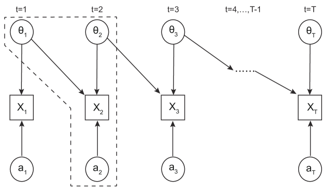
Figure 9: DAG representation of the sequential Gaussian regression model. The dashed area highlights one self-contained Bayesian module $\Psi_{2}=(\theta_{1},\theta_{2},a_{2},X_{2})$.

Suppose the true data generating process is according to the DAG as shown in Figure 9. At each time $t=1,\cdots,T$, we have an $n$-dimensional observation $X_{t}=(X_{t1},\cdots,X_{tn})$ with the following true data generating process:

$$X_{1}|\nu_{1} \sim\mathcal{N}\left(P_{1}\nu_{1},\textbf{I}\right);$$ (8)

$$X_{t}|\nu_{t},\theta_{t-1} \sim\mathcal{N}\left(P_{t}\nu_{t}+Q_{t}f^{\ast}(\theta_{t-1}),\textbf{I}\right),\qquad t=2,3,\dots$$

Here, $\theta_{t}$, $t=1,\cdots,T$, is the parameter of interest and let $\nu_{t}=(a_{t},\theta_{t})^{\mathsf{T}}$, $t=1,\cdots,T$ be the augmented parameter which includes an additional intercept term $a_{t}$; and $f^{\ast}(\cdot)$ is an unknown deterministic function in the true data generating process. The current covariate matrix $P_{t}$ is:

$$P_{t}=\begin{pmatrix}1&p_{t1}\\ 1&p_{t2}\\ \vdots&\vdots\\ 1&p_{tn}\end{pmatrix};$$

and the past covariate vector is $Q_{t}=(q_{t1},\cdots,q_{tn})$, $t=2,3,\dots$. We further assume that $p_{tk}$ and $q_{tk}$ are realizations of covariate variables, which have been drawn independently with mean 0. The 0 mean assumption is plausible because we can always centralize $P_{t}$ and $Q_{t}$ and this centralization can be compensated by the intercept parameter $a_{t}$. The covariance matrix is assumed to be the identity matrix I for simplicity.

We now suppose the true data generating process is partially unknown. Specifically we assume the function $f^{\ast}(\cdot)$ is unknown, and that the analysis model is misspecified as $f(\cdot)=f^{\ast}(\cdot)+\delta$, where $\delta$ quantifies the degree of misspecification.

In this Section we will calculate and compare the estimation bias when using cut inference and using standard Bayesian inference. To make the cut distribution tractable, we use the conjugate prior $\nu_{t}\sim\mathcal{N}(0,\textbf{I})$.

3.3.1 Cut inference

We first consider applying the cut inference and show that the estimation bias will approximately be 0 on an average basis with respect to realizations of $P_{t}$ and $Q_{t}$. The idea is that, at every time $t$, we cut the feedback from time $t+1$ so that misspecification beyond $t+1$ will not affect the inference before that time.

For now, assume that the misspecification of $f^{\ast}(\cdot)$ only exists between time $t-1$ and $t$ for a specific time $0<t<T$ (we will relax this assumption later). To form modules, we first partition the observable random variables $X=(X_{1},\cdots,X_{T})$ into two disjoint groups $X_{A}^{\ast}=(X_{1},\cdots,X_{t-1})$ and $X_{B}^{\ast}=(X_{t},\cdots,X_{T})$. Then by Rule 1, we have two self-contained Bayesian modules $\Phi_{A}=(\theta_{1},\cdots,\theta_{t-1},\allowbreak a_{1},\cdots,a_{t-1},\allowbreak X_{1},\cdots,X_{t-1})$ and $\Phi_{B}=(\theta_{t-1},\cdots,\theta_{T},a_{t},\cdots,a_{T},X_{t},\cdots,X_{T})$. Because the misspecification relates to the function $f^{\ast}(\cdot)$ which links observations at time $t-1$ and $t$, we wish to prevent information from time $t,t+1,\cdots T$ being used, which will avoid bias for inference before time $t$. Hence, we choose module $B$ to be the child module.

First, note there is no misspecification before time $t-1$ and thus a standard Bayesian inference for $(\nu_{1},\cdots,\nu_{t-1})$ with information only from module $A$ can be conduct. This is available because module $A$ is a self-contained Bayesian module. Second, to calculate the estimation bias at time $t$, we split module $B$ into two modules $\Psi_{C}=(\theta_{t-1},\theta_{t},a_{t},X_{t})$ and $\Phi_{D}=(\theta_{t},\cdots,\theta_{T},a_{t+1},\cdots,a_{T},X_{t+1},\cdots,X_{T})$ and similarly treat module $D$ as the child module of module $C$ (i.e., we have the order $A\rightharpoonup C\rightharpoonup D$). To simplify the notation, we write

$$\Lambda_{t}=P_{t}^{\mathsf{T}}P_{t}+\textbf{I}=\begin{pmatrix}n+1&\sum p_{ti}\\ \sum p_{ti}&\sum p_{ti}^{2}+1\end{pmatrix}$$

Now by Definition 5 (case: $A\rightharpoonup C\rightharpoonup D$), the conditional self-contained Bayesian posterior of $\nu_{t}$, conditional on $\theta_{t-1}$, is

$$\nu_{t}|X_{t},\theta_{t-1}\sim\mathcal{N}\left(\Lambda_{t}^{-1}P_{t}^{\mathsf{T}}(X_{t}-Q_{t}f(\theta_{t-1})),\ \Lambda_{t}^{-1}\right),$$

where $f(\cdot)$ is the misspecified function such that $f(\cdot)=f^{\ast}(\cdot)+\delta$, and thus

$$\nu_{t}|X_{t},\theta_{t-1}\sim\mathcal{N}\left(\Lambda_{t}^{-1}P_{t}^{\mathsf{T}}(X_{t}-Q_{t}f^{\ast}(\theta_{t-1}))-\Lambda_{t}^{-1}P_{t}^{\mathsf{T}}Q_{t}\delta,\ \Lambda_{t}^{-1}\right).$$ (9)

It is clear that the estimation bias is $\Delta_{t}=K_{t}\delta$, where $K_{t}:=\Lambda_{t}^{-1}P_{t}^{\mathsf{T}}Q_{t}$. Since

$$\Lambda_{t}^{-1}=\frac{1}{(n+1)(\sum p_{ti}^{2}+1)-(\sum p_{ti})^{2}}\begin{pmatrix}\sum p_{ti}^{2}+1&-\sum p_{ti}\\ -\sum p_{ti}&n+1\end{pmatrix},$$

the estimation bias for the intercept $a=(a_{1},\cdots,a_{T})$ is

$$K_{t1}=\frac{(\sum p_{ti}^{2}+1)\sum q_{ti}-\sum p_{ti}\sum p_{ti}q_{ti}}{(n+1)(\sum p_{ti}^{2}+1)-(\sum p_{ti})^{2}};$$

and the estimation bias for the parameter of interest $(\theta_{1},\cdots,\theta_{T})$ is

$$K_{t2}=\frac{(n+1)\sum p_{ti}q_{ti}-\sum p_{ti}\sum q_{ti}}{(n+1)(\sum p_{ti}^{2}+1)-(\sum p_{ti})^{2}}.$$

Both $K_{t1}$ and $K_{t2}$ have mean 0 so the estimation bias will distribute around 0.

Now we consider the case when the function $f^{\ast}(\cdot)$ is misspecified for all $t$ meaning that we would like to cut feedback between all times $t$ and $t+1$. We therefore recursively split the modules until each module involves a single observable random variable. In other words, given the partition of observable random variable as: $X_{t}^{\ast}=X_{t}$ for $t=1,\cdots,T$, by Rule 1, we have modules $\Psi_{1}=(\theta_{1},a_{1},X_{1})$ and $\Psi_{t}=(\theta_{t-1},\theta_{t},a_{t},X_{t})$ for $t>1$ as shown in Figure 9. Similarly, we can let $\Psi_{t+1}$ be the child module of $\Psi_{t}$ by Rule 2 because there is a direct edge $\theta_{t}\rightarrow X_{t+1}$ (see Figure 9) for all $t$. Note that estimation bias could still accumulate for future modules (i.e., descendant modules). Denote $\theta_{t}^{\ast}$ as the true value of $\theta_{t}$ and $\nu_{t}^{\ast}$ as the true value of $\nu_{t}$ for any $t$. Consider the estimation bias at time $t=2$, based on (9). Since module $\Psi_{1}$ does not involve any misspecification, the conditional self-contained Bayesian posterior of $\nu_{1}$ has mean $\nu_{1}^{\ast}$, we can write

$$\mathbb{E}_{\theta_{1}}\left(\mathbb{E}(\nu_{2}|X_{2},\theta_{1})\right)=\nu_{2}^{\ast}-K_{2}\delta.$$

Then based on (9), it is easy to deduce that

$$\mathbb{E}(\nu_{3}|X_{3},\theta_{2}) =\Lambda_{3}^{-1}P_{3}^{\mathsf{T}}(X_{3}-Q_{3}f^{\ast}(\theta_{2}))-K_{3}\delta;$$

$$\mathbb{E}_{\theta_{2}}\left(\mathbb{E}(\nu_{3}|X_{3},\theta_{2})\right) =\mathbb{E}_{\theta_{2}}\left(\Lambda_{3}^{-1}P_{3}^{\mathsf{T}}(X_{3}-Q_{3}f^{\ast}(\theta_{2}))\right)-K_{3}\delta$$

$$\approx\mathbb{E}_{\theta_{2}}\left(\Lambda_{3}^{-1}P_{3}^{\mathsf{T}}\{X_{3}-Q_{3}[f^{\ast}(\theta_{2}^{\ast})+{f^{\ast}}^{\prime}(\theta_{2}^{\ast})(\theta_{2}-\theta_{2}^{\ast})]\}\right)-K_{3}\delta$$

$$=\left(\Lambda_{3}^{-1}P_{3}^{\mathsf{T}}(X_{3}-Q_{3}f^{\ast}(\theta_{2}^{\ast}))\right)+\Lambda_{3}^{-1}P_{3}^{\mathsf{T}}Q_{3}{f^{\ast}}^{\prime}(\theta_{2}^{\ast})K_{22}\delta-K_{3}\delta$$

$$=\left(\Lambda_{3}^{-1}P_{3}^{\mathsf{T}}(X_{3}-Q_{3}f^{\ast}(\theta_{2}^{\ast}))\right)-K_{3}(1-{f^{\ast}}^{\prime}(\theta_{2}^{\ast})K_{22})\delta.$$

Hence, the estimation bias, up to module 3, is approximately equal to $K_{3}(1-{f^{\ast}}^{\prime}(\theta_{2}^{\ast})K_{22})\delta$. Similarly, we have

$$\mathbb{E}_{\theta_{2}}\cdots\mathbb{E}_{\theta_{t-1}}\left(\mathbb{E}(\nu_{t}|X_{t},f(\theta_{t-1}))\right) \approx\left(\Lambda_{t}^{-1}P_{t}^{\mathsf{T}}(X_{t}-Q_{t}f^{\ast}(\theta_{t-1}^{\ast}))\right)$$

$$-K_{t}\left(1-\sum_{i=1}^{t-2}\{(-1)^{i+1}\prod_{j=t-i}^{t-1}[{f^{\ast}}^{\prime}(\theta_{j}^{\ast})K_{j2}]\}\right)\delta$$

Comparing with the original estimation bias $\Delta_{t}=K_{t}\delta$ when accumulation of bias is not considered, we observe that the estimation bias is perturbed by a multiplier $(1-\Upsilon_{t-1})$, where

$$\Upsilon_{t-1}:=\sum_{i=1}^{t-2}\{(-1)^{i+1}\prod_{j=t-i}^{t-1}[{f^{\ast}}^{\prime}(\theta_{j}^{\ast})K_{j2}]\}.$$

Note that $(1-\Upsilon_{t-1})$ has mean 1 since $K_{j2}$ has mean 0 for all $1\leq j\leq T$ and they are independent with each other. Hence, the mean (in terms of $P_{t}$ and $Q_{t}$) of the estimation bias is still 0 when function $f^{\ast}(\cdot)$ is misspecified for all $t$ .

3.3.2 Standard Bayesian inference with estimation bias

Now we derive the standard posterior distribution for this model. Suppose for now that we perform inference under the correctly specified mode. We can approximate the true data generating process (8), for any $t>1$, by Taylor approximation as a function of $\theta_{t-1}^{\star}$, which is a known “guess” of $\theta_{t-1}$ that is close to the true value:

$$X_{t}|\nu_{t},\theta_{t-1}\mathchoice{\mathrel{\ooalign{$\displaystyle\sim$\cr$\displaystyle.$\cr\raise 3.87498pt\hbox{$\displaystyle.$}\cr}}}{\mathrel{\ooalign{$\textstyle\sim$\cr$\textstyle.$\cr\raise 3.87498pt\hbox{$\textstyle.$}\cr}}}{\mathrel{\ooalign{$\scriptstyle\sim$\cr$\scriptstyle.$\cr\raise 2.71246pt\hbox{$\scriptstyle.$}\cr}}}{\mathrel{\ooalign{$\scriptscriptstyle\sim$\cr$\scriptscriptstyle.$\cr\raise 1.93748pt\hbox{$\scriptscriptstyle.$}\cr}}}\mathcal{N}\left(P_{t}\nu_{t}+Q_{t}f^{\ast}(\theta_{t-1}^{\star})+Q_{t}{f^{\ast}}^{\prime}(\theta_{t-1}^{\star})(\theta_{t-1}-\theta_{t-1}^{\star}),\textbf{I}\right).$$

Writing $\tilde{X}_{t}:=X_{t}-Q_{t}f^{\ast}(\theta_{t-1}^{\star})+Q_{t}{f^{\ast}}^{\prime}(\theta_{t-1}^{\star})\theta_{t-1}^{\star}$ and $m_{t-1}^{\ast}={f^{\ast}}^{\prime}(\theta_{t-1}^{\star})$ for $t>1$, this can be simplified as

$$\tilde{X}_{t}|\nu_{t},\theta_{t-1}\mathchoice{\mathrel{\ooalign{$\displaystyle\sim$\cr$\displaystyle.$\cr\raise 3.87498pt\hbox{$\displaystyle.$}\cr}}}{\mathrel{\ooalign{$\textstyle\sim$\cr$\textstyle.$\cr\raise 3.87498pt\hbox{$\textstyle.$}\cr}}}{\mathrel{\ooalign{$\scriptstyle\sim$\cr$\scriptstyle.$\cr\raise 2.71246pt\hbox{$\scriptstyle.$}\cr}}}{\mathrel{\ooalign{$\scriptscriptstyle\sim$\cr$\scriptscriptstyle.$\cr\raise 1.93748pt\hbox{$\scriptscriptstyle.$}\cr}}}\mathcal{N}\left(P_{t}\nu_{t}+Q_{t}m_{t-1}^{\ast}\theta_{t-1},\textbf{I}\right).$$

Let $0_{n\times 2}$ denote a 0 matrix with $n$ rows and $2$ columns and let

$$\tilde{Q}_{t}=\begin{pmatrix}0&p_{t1}\\ \vdots&\vdots\\ 0&p_{tn}\end{pmatrix}$$

Then we can write the mean of $\tilde{X}$ in the matrix form as:

$$\mathbb{E}\left[\begin{pmatrix}\tilde{X}_{1}\\ \tilde{X}_{2}\\ \tilde{X}_{3}\\ \vdots\\ \tilde{X}_{T}\end{pmatrix}\right]=\mathbb{E}(\tilde{X})\approx B\nu=\begin{pmatrix}P_{1}&0_{n\times 2}&0_{n\times 2}&\cdots&0_{n\times 2}&0_{n\times 2}\\ \tilde{Q}_{2}m_{1}^{\ast}&P_{2}&0_{n\times 2}&\cdots&0_{n\times 2}&0_{n\times 2}\\ 0_{n\times 2}&\tilde{Q}_{3}m_{2}^{\ast}&P_{3}&\cdots&0_{n\times 2}&0_{n\times 2}\\ \vdots&\vdots&\vdots&\ddots&\vdots&\vdots\\ 0_{n\times 2}&0_{n\times 2}&0_{n\times 2}&\cdots&\tilde{Q}_{T}m_{T-1}^{\ast}&P_{T}\end{pmatrix}\begin{pmatrix}\nu_{1}\\ \nu_{2}\\ \nu_{3}\\ \vdots\\ \nu_{T}\end{pmatrix}$$

The standard posterior distribution of $\nu$ under the conjugate prior, when there is no misspecification (i.e., when $f^{\ast}(\cdot)$ is used), is

$$\nu|\tilde{X}\mathchoice{\mathrel{\ooalign{$\displaystyle\sim$\cr$\displaystyle.$\cr\raise 3.87498pt\hbox{$\displaystyle.$}\cr}}}{\mathrel{\ooalign{$\textstyle\sim$\cr$\textstyle.$\cr\raise 3.87498pt\hbox{$\textstyle.$}\cr}}}{\mathrel{\ooalign{$\scriptstyle\sim$\cr$\scriptstyle.$\cr\raise 2.71246pt\hbox{$\scriptstyle.$}\cr}}}{\mathrel{\ooalign{$\scriptscriptstyle\sim$\cr$\scriptscriptstyle.$\cr\raise 1.93748pt\hbox{$\scriptscriptstyle.$}\cr}}}\mathcal{N}(\Lambda^{-1}B^{\mathsf{T}}\tilde{X},\Lambda),$$

where $\Lambda=(B^{\mathsf{T}}B+I)$ and can be interpreted as a block matrix

$$\pNiceMatrix\Lambda_{1}^{(1)}&\Lambda_{2}^{(2)}0_{2\times 2}\Cdots 0_{2\times 2}\\ \Lambda_{2}^{(2)}\Ddots\Ddots\Ddots\Vdots\\ 0_{2\times 2}\Ddots\\ \Vdots\Ddots 0_{2\times 2}\\ \Lambda_{T}^{(2)}\\ 0_{2\times 2}\Cdots 0_{2\times 2}\Lambda_{T}^{(2)}\Lambda_{T}^{(1)}$$

where

$$\Lambda_{t}^{(1)}=\begin{pmatrix}n+1&\sum_{i=1}^{n}p_{ti}\\ \sum_{i=1}^{n}p_{ti}&\sum_{i=1}^{n}(p_{ti}^{2}+(m_{t}^{\ast}q_{(t+1)i})^{2})+1\end{pmatrix}\ \ \ \text{for}\ t<T;$$

$$\Lambda_{T}^{(1)}=\begin{pmatrix}n+1&\sum_{i=1}^{n}p_{Ti}\\ \sum_{i=1}^{n}p_{Ti}&\sum_{i=1}^{n}p_{Ti}^{2}+1\end{pmatrix};$$

$$\Lambda_{t}^{(2)}=\pNiceMatrix 0&0\\ 0m_{t-1}^{\ast}\sum_{i=1}^{n}(p_{ti}q_{ti})\ \ \ \text{for}\ t>1;$$

However, the model that we actually use is misspecified, with $f(\cdot)=f^{\ast}(\cdot)+\delta$. Under this misspecification, the standard posterior distribution is:

$$\nu|\tilde{X}\mathchoice{\mathrel{\ooalign{$\displaystyle\sim$\cr$\displaystyle.$\cr\raise 3.87498pt\hbox{$\displaystyle.$}\cr}}}{\mathrel{\ooalign{$\textstyle\sim$\cr$\textstyle.$\cr\raise 3.87498pt\hbox{$\textstyle.$}\cr}}}{\mathrel{\ooalign{$\scriptstyle\sim$\cr$\scriptstyle.$\cr\raise 2.71246pt\hbox{$\scriptstyle.$}\cr}}}{\mathrel{\ooalign{$\scriptscriptstyle\sim$\cr$\scriptscriptstyle.$\cr\raise 1.93748pt\hbox{$\scriptscriptstyle.$}\cr}}}\mathcal{N}\left(\Lambda^{-1}B^{\mathsf{T}}\tilde{X}-\Lambda^{-1}B^{\mathsf{T}}\begin{pmatrix}0_{n\times 1}\\ Q_{2}\\ \vdots\\ Q_{T}\end{pmatrix}\delta,\Lambda\right),$$

where

$$B^{\mathsf{T}}\begin{pmatrix}0_{n\times 1}\\ Q_{2}\\ \vdots\\ Q_{T}\end{pmatrix}=\begin{pmatrix}0\\ \sum(q_{2i}m_{1}^{\ast})^{2}\\ m_{1}^{\ast}\sum q_{2i}\\ m_{1}^{\ast}\sum p_{2i}q_{2i}+\sum(q_{3i}m_{2}^{\ast})^{2}\\ \vdots\\ m_{T-1}^{\ast}\sum q_{Ti}\\ m_{T-1}^{\ast}\sum p_{Ti}q_{Ti}.\end{pmatrix}$$

Unlike when using cut inference, there are no guarantees that the estimation bias $\Delta$ defined as

$$\Delta:=\Lambda^{-1}B^{\mathsf{T}}\begin{pmatrix}0_{n\times 1}\\ Q_{2}\\ \vdots\\ Q_{T}\end{pmatrix}\delta$$

has a mean (in terms of $P_{t}$ and $Q_{t}$) 0. Therefore, the estimation bias may not distribute around 0. An example of this is shown in the the numerical simulation in the supplementary materials.

4 Conclusion

In this paper, we have formulated rules that describe how to apply cut inference within a modularized Bayesian framework. In particular, we formally define a “module”, which we refer to as a “self-contained Bayesian module”, as the set of variables, associated with a set of observable random variables, that can be used to conduct standard Bayesian inference for the module. We provide a rule prescribing how to form a self-contained Bayesian module from the structure of the DAG, starting from a partition of observable random variables. We describe the internal relationship between modules as a “parent-child ordering” in which inference of a child module is affected by its parent module (ancestor modules in multiple-module case) according to conditional self-contained Bayesian inference. This order can be identified directly from the DAG. Finally, we formulate the associated cut distributions, spanning from the basic two-module case to a more complicated multiple-module case. The extension of cut inference from a two-module case to multiple-module case is available via our sequential splitting technique.

We define self-contained Bayesian module in terms of the observable random variables rather than the parameters. There is a short and incomplete proposal of the definition of the cut inference via a Gibbs sampling scheme which concentrates on the parameters (Yu et al., , 2021). The idea is that the factorized joint distribution (1) can be viewed as a product of factors that involve parameters. For example, a likelihood $p(\theta|pa(\theta))$ can be regarded as a factor $f(\theta,\Theta\cap pa(\theta))$ which involves parameter $\theta$ and $\Theta\cap pa(\theta)$. The standard Gibbs sampler draws samples of a particular $\theta$ from its full conditional density $p(\theta|(\Theta\setminus\theta))$ which is proportional to the product of all factors that involve this $\theta$. To conduct cut inference for this $\theta$ when a particular factor is misspecified, they derive a new modified conditional density $p_{\text{cut}}(\theta|(\Theta\setminus\theta))$ for $\theta$ by dropping the misspecified factor in the product. This proposal of cut inference is inspiring because it focuses on the parameter of interest and may work well for the generic two-module case. However, direct extension of this definition to the multiple-module case is unclear. It is not clear how to handle the varying degrees of partial misspecification across modules (or in the factors according to the definition of Yu et al., (2021)) which is common in a multiple-module case. Furthermore, it is unclear how to determine which order to drop factors when there are multiple misspecified factors. We expect more discussions of this definition and studies of the possible inherent link with our definition in the future.

Studies of the cut inference within the generic two-module case are drawing broad attention recently. These include studies of the sampling methods for cut distribution (Plummer, , 2015; Jacob et al., , 2020; Yu et al., , 2021; Liu and Goudie, , 2022), the selection between cut distribution and standard posterior distribution (Jacob et al., , 2017), the asymptotic properties of cut distribution (Pompe and Jacob, , 2021), the extension of cut inference for likelihood-free inference (Chakraborty et al., , 2022), the extension of cut inference for generalized Bayesian inference (Frazier and Nott, , 2022) and the application of cut distributions in semi-parametric hidden Markov models (Moss and Rousseau, , 2022). These studies are based on the generic two-module case, and extension of their results to a general multiple-module case remains unclear and may not be straightforward. We hope that this study can conceptualize cut inference for a broader range of statistical models, and enlighten future developments of methodology and algorithm, and stimulate applications of modularized Bayesian inference.

Supplementary Materials

The appendix contains all technical proofs and simulated results stated in the paper.

Appendix A Proofs

A.1 Proof of Lemma 1

1. Given Rule 1, it is straightforward to conclude that $\Psi_{(A\cup B)^{\mathsf{c}}}$ only contains parameters. This is because all observables will be in either $X_{A}$ or $X_{B}$ (or both) since $X=X_{A}^{\ast}\cup X_{B}^{\ast}$ is a partition of the observables.

   Now, suppose there is an edge $\psi_{(A\cup B)^{\mathsf{c}}}\rightarrow x_{A\cup B}$, where $x_{A\cup B}\in X_{A\cup B}$ and $\psi_{(A\cup B)^{\mathsf{c}}}\in\Psi_{(A\cup B)^{\mathsf{c}}}$. By Rule 1, we must incorporate $\psi_{(A\cup B)^{\mathsf{c}}}$ into either module $A$ or module $B$. This contradicts the fact that $\psi_{(A\cup B)^{\mathsf{c}}}\in\Psi_{(A\cup B)^{\mathsf{c}}}$.

   Now suppose there is an edge $\psi_{(A\cup B)^{\mathsf{c}}}\rightarrow\theta_{A\cup B}$, where $\theta_{A\cup B}\in\Theta_{A\cup B}$ and $\psi_{(A\cup B)^{\mathsf{c}}}\in\Psi_{(A\cup B)^{\mathsf{c}}}$. By Rule 1, $\theta_{A\cup B}$ must have a descendant $x^{\ast}\in X$ such that there is at least one directed path between $x^{\ast}=\psi_{1},\cdots,\psi_{s}=\theta_{A\cup B}$ with $x^{\ast}$ as the leaf and every $\psi_{l}\in\Theta$, $l>1$. Then by Rule 1 we must incorporate $\psi_{(A\cup B)^{\mathsf{c}}}$ into the module associated with this $x^{\ast}$. This contradicts the fact that $\psi_{(A\cup B)^{\mathsf{c}}}\in\Psi_{(A\cup B)^{\mathsf{c}}}$.

2. Let $\psi_{A\setminus B}\leftarrow\psi^{\ast}$ be an edge where $\psi_{A\setminus B}\in\Psi_{A\setminus B}$ and $\psi^{\ast}\notin\Psi_{A\setminus B}$. By the first statement of Lemma 1, $\psi^{\ast}\notin\Psi_{(A\cup B)^{\mathsf{c}}}$. By Rule 1, we must incorporate $\psi^{\ast}$ into module $A$, so it must belong to $\Psi_{A\cap B}$.

   Now let $\psi_{A\setminus B}\rightarrow\psi^{\ast}$ be an edge where $\psi_{A\setminus B}\in\Psi_{A\setminus B}$ and $\psi^{\ast}\notin\Psi_{A\setminus B}$. If $\psi^{\ast}\in\Psi_{B\setminus A}$, by Rule 1 we must incorporate $\psi_{A\setminus B}$ into module $B$. This has contradicted the fact that $\psi_{A\setminus B}\in\Psi_{A\setminus B}$. Hence, $\psi^{\ast}$ can only belong to either $\Psi_{A\cap B}$ or $\Psi_{(A\cup B)^{\mathsf{c}}}$.

3. Consider a V-structure $\psi_{A\setminus B}\rightarrow x_{A\cap B}\leftarrow\psi_{B\setminus A}$ where $x_{A\cap B}\in X_{A\cap B}$. Now $x_{A\cap B}$ must belong to either $X_{A}^{\ast}$ or $X_{B}^{\ast}$. Suppose $x_{A\cap B}\in X_{A}^{\ast}$, then by Rule 1, we must incorporate both $\psi_{A\setminus B}$ and $\psi_{B\setminus A}$ into module A, which leads to a contradiction. The corresponding argument applies if $x_{A\cap B}\in X_{B}^{\ast}$.

   If there is a V-structure $\psi_{A\setminus B}\rightarrow\theta_{A\cap B}\leftarrow\psi_{B\setminus A}$ where $\theta_{A\cap B}\in\Theta_{A\cap B}$, then $\theta_{A\cap B}$ must have a descendant $x_{A}\in X_{A}^{\ast}$ such that there is at least one directed path between $\theta_{A\cap B}=\psi_{1},\cdots,\psi_{s}=x_{A}$ with $x_{A}$ as the leaf and every $\psi_{l}\in\Theta$, $l<s$. By Rule 1 we must incorporate $\psi_{A\setminus B}$ and $\psi_{B\setminus A}$ into module $A$ and this leads to a contradiction.

4. We first consider $\text{pa}(\Theta_{A\cap B})$. By Rule 1, any parent node $\psi\in\text{pa}(\Theta_{A\cap B})$ must also have descendants both in $X_{A}^{\ast}$ and $X_{B}^{\ast}$. Therefore, this $\psi$ belongs to both module $A$ and $B$. Because $\psi\notin\Theta_{A\cap B}$ by the definition of $\text{pa}(\cdot)$, then $\psi\in X_{A\cap B}$.

   We then consider $\text{pa}(X_{A\cap B})$. By the first statement of Lemma 1, $\text{pa}(X_{A\cap B})\cap\Psi_{(A\cup B)^{\mathsf{c}}}=\emptyset$. Then $\text{pa}(X_{A\cap B})\subseteq\Psi\setminus\left(\Psi_{(A\cup B)^{\mathsf{c}}}\cup X_{A\cap B}\right)$. It is clear that $\Psi\setminus\left(\Psi_{(A\cup B)^{\mathsf{c}}}\cup X_{A\cap B}\right)=\{\Theta_{A\cap B},\Theta_{A\setminus B},\Theta_{B\setminus A},X_{A\setminus B},X_{B\setminus A}\}$.

5. We first consider the case when $\Psi_{(A\cup B)^{\mathsf{c}}}$-cut-sub-graph $G_{\text{cut}(\Psi_{(A\cup B)^{\mathsf{c}}})}$ has two disconnected components which are formed separately by nodes $\Psi_{A}$ and $\Psi_{B}$. If $\Psi_{A\cap B}\neq\emptyset$, then there must exist at least one $\psi\in\Psi_{A\cap B}$ which is the common ancestor of $X_{A}^{\ast}\subseteq\Psi_{A}$ and $X_{B}^{\ast}\subseteq\Psi_{B}$ by Rule 1. Hence $\Psi_{A}$ is connected with $\Psi_{B}$ which leads to a contradiction.

   We then consider the case when $\Psi_{A\cap B}=\emptyset$. If nodes $\Psi_{A}$ and $\Psi_{B}$ are connected in $\Psi_{(A\cup B)^{\mathsf{c}}}$-cut-sub-graph $G_{\text{cut}(\Psi_{(A\cup B)^{\mathsf{c}}})}$, because there is no edge between $\Psi_{A\cup B}$ and $\Psi_{(A\cup B)^{\mathsf{c}}}$ in $G_{\text{cut}(\Psi_{(A\cup B)^{\mathsf{c}}})}$, then there must be at least one edge $\psi_{1}\rightarrow\psi_{2}$ where $\psi_{1}\in\Psi_{A}$ and $\psi_{2}\in\Psi_{B}$ (or $\psi_{1}\in\Psi_{B}$ and $\psi_{2}\in\Psi_{A}$). Because $\psi_{1}\in\Psi_{A}$, then there must be a directed path $\psi_{1}\rightsquigarrow x_{a}$ where $x_{a}\in X_{A}^{\ast}$ by Rule 1. Similarly, because $\psi_{2}\in\Psi_{B}$, there must be a directed path $\psi_{2}\rightsquigarrow x_{b}$ where $x_{b}\in X_{B}^{\ast}$ by Rule 1. Now we have that there are both $\psi_{1}\rightsquigarrow x_{a}$ and $\psi_{1}\rightsquigarrow x_{b}$, then by Rule 1 we must include this $\psi_{1}$ into $\Psi_{A\cap B}$ which leads to a contradiction.

A.2 Proof of Lemma 2

We give a proof by contraction. Suppose $\Psi_{A\setminus B}$ and $\Psi_{B\setminus A}$ are d-connected by $\Psi_{A\cap B}$. This indicates that there exists an undirected path $U$: $\psi_{A\setminus B}=\psi_{1},\cdots,\psi_{s}=\psi_{B\setminus A}$ between $\Psi_{A\setminus B}$ and $\Psi_{B\setminus A}$ such that for every collider $\psi_{l}$ on this path $U$, either $\psi_{l}$ or a descendent of $\psi_{l}$ is in $\Psi_{A\cap B}$, and no non-collider on this path $U$ is in $\Psi_{A\cap B}$. By the second statement of Lemma 1, we conclude that there is no edge that links $\Psi_{A\setminus B}$ and $\Psi_{B\setminus A}$. Hence, all undirected paths that link $\Psi_{A\setminus B}$ and $\Psi_{B\setminus A}$ go through nodes in $\Psi_{A\cap B}\cup\Psi_{(A\cup B)^{\mathsf{c}}}$.

If path $U$ does not involve any node from $\Psi_{(A\cup B)^{\mathsf{c}}}$, because of the $d-connection$ by $\Psi_{A\cap B}$, there must be a V-structure $\psi_{l-1}\rightarrow\psi_{l}\leftarrow\psi_{l+1}$ on path $U$ where $\psi_{l}\in\Psi_{A\cap B}$, $\psi_{l-1}\in\Psi_{A\setminus B}$ and $\psi_{l+1}\in\Psi_{B\setminus A}$. This has contradicted the third statement of Lemma 1.

If path $U$ involves nodes from $\Psi_{(A\cup B)^{\mathsf{c}}}$, by the first statement of Lemma 1, there must be a fragment of path $U$: $a=\psi_{s_{1}},\psi_{s_{1}+1},\cdots,\psi_{s_{2}}=b$, $s_{1}\geq 1$ and $s_{2}\leq s$, that satisfies $(\psi_{s_{1}},\psi_{s_{2}})\in\Psi_{(A\cup B)}$, $(\psi_{s_{1}+1},\cdots,\psi_{s_{2}-1})\in\Psi_{(A\cup B)^{\mathsf{c}}}$, $\psi_{s_{1}}\rightarrow\psi_{s_{1}+1}$ and $\psi_{s_{2}}\rightarrow\psi_{s_{2}-1}$. Hence, there must be a V-structure $\psi_{l-1}\rightarrow\psi_{l}\leftarrow\psi_{l+1}$ on this fragment. Because of the $d-connection$ by $\Psi_{A\cap B}$, a descendent of $\psi_{l}\in\Psi_{(A\cup B)^{\mathsf{c}}}$ is in $\Psi_{A\cap B}$. This has contradicted the fact that $\text{ch}(\Psi_{(A\cup B)^{\mathsf{c}}})=\emptyset$ (i.e., a descendent of $\psi_{l}\in\Psi_{(A\cup B)^{\mathsf{c}}}$ must be in $\Psi_{(A\cup B)^{\mathsf{c}}}$).

In summary, we have proved that the $d-connection$ between $\Psi_{A\setminus B}$ and $\Psi_{B\setminus A}$ by $\Psi_{A\cap B}$ does not hold. Hence, $\Psi_{A\setminus B}$ and $\Psi_{B\setminus A}$ are d-separated by $\Psi_{A\cap B}$ and we have

$$\Psi_{A\setminus B}\raisebox{0.45003pt}{\rotatebox[origin={c}]{90.0}{$\models$}}\Psi_{B\setminus A}|\Psi_{A\cap B}.$$

A.3 Proof of Theorem 1

We prove the Theorem for $\Psi_{A}$: the proof for $\Psi_{B}$ is the same due to symmetry. Given $X_{A}^{\ast}$, Rule 1 indicates that the $X_{A}^{\ast}$-associated observables $X_{X_{A}^{\ast}}=X_{A\cap B}\cap X_{B}^{\ast}$ and the $X_{A}^{\ast}$-associated parameters $\Theta_{X_{A}^{\ast}}=\Theta_{A}$ (the parameter of interest to infer the true data generating process of $X_{A}^{\ast}$). By Definition 2, we need to build a posterior distribution $p(\Theta_{A}|X_{A}^{\ast},X_{A\cap B}\cap X_{B}^{\ast})$ in order to prove $\Phi_{A}=(\Theta_{A},X_{A})$ is a minimally self-contained Bayesian module with respect to $X_{A}^{\ast}$.

Given the DAG in which $\Psi_{A}$ and $\Psi_{B}$ are formed via Rule 1, by Lemma 1 and Lemma 2, we can write the distribution of each set of variables as follows:

$$p(\Theta_{A\setminus B}|\text{pa}(\Theta_{A\setminus B}));\ \ \text{pa}(\Theta_{A\setminus B})\subseteq\{\Theta_{A\cap B},X_{A\setminus B},X_{A\cap B}\};$$

$$p(\Theta_{A\cap B}|\text{pa}(\Theta_{A\cap B}));\ \ \text{pa}(\Theta_{A\cap B})\subseteq X_{A\cap B}$$

$$p(X_{A\setminus B}|\text{pa}(X_{A\setminus B}));\ \ \text{pa}(X_{A\setminus B})\subseteq\{\Theta_{A\setminus B},\Theta_{A\cap B},X_{A\cap B}\}$$

$$p(X_{A\cap B}|\text{pa}(X_{A\cap B}));\ \ \text{pa}(X_{A\cap B})\subseteq\{\Theta_{A\cap B},\Theta_{A\setminus B},\Theta_{B\setminus A},X_{A\setminus B},X_{B\setminus A}\}$$

$$p(X_{B\setminus A}|\text{pa}(X_{B\setminus A}));\ \ \text{pa}(X_{B\setminus A})\subseteq\{\Theta_{B\setminus A},\Theta_{A\cap B},X_{A\cap B}\}$$

$$p(\Theta_{B\setminus A}|\text{pa}(\Theta_{B\setminus A}));\ \ \text{pa}(\Theta_{B\setminus A})\subseteq\{\Theta_{A\cap B},X_{B\setminus A},X_{A\cap B}\}$$

$$p(\Theta_{(A\cup B)^{\mathsf{c}}}|\text{pa}(\Theta_{(A\cup B)^{\mathsf{c}}}));\ \ \text{pa}(\Theta_{(A\cup B)^{\mathsf{c}}})\subseteq\{\Theta_{A\cup B},X\}.$$

Note that, because $X=X_{A}^{\ast}\cup X_{B}^{\ast}$, the distribution of $X_{A\cap B}$ can be split into

$$p(X_{A\cap B}|\text{pa}(X_{A\cap B}))=p(X_{A\cap B}\cap X_{A}^{\ast}|\text{pa}(X_{A\cap B}\cap X_{A}^{\ast}))p(X_{A\cap B}\cap X_{B}^{\ast}|\text{pa}(X_{A\cap B}\cap X_{B}^{\ast})).$$

Because $\text{pa}(X_{A}^{\ast})\cap\Psi_{B\setminus A}=\emptyset$ and $\text{pa}(X_{B}^{\ast})\cap\Psi_{A\setminus B}=\emptyset$, we can write

$$\text{pa}(X_{A\cap B}\cap X_{A}^{\ast}) \subseteq\{\Theta_{A\cap B},\Theta_{A\setminus B},X_{A\setminus B},X_{A\cap B}\cap X_{B}^{\ast}\}$$

$$\text{pa}(X_{A\cap B}\cap X_{B}^{\ast}) \subseteq\{\Theta_{A\cap B},\Theta_{B\setminus A},X_{B\setminus A},X_{A\cap B}\cap X_{A}^{\ast}\}.$$

Now given these distributions, one posterior distribution for $\Theta_{A}$ is simply the standard posterior distribution using all observables. That is:

$$p(\Theta_{A}|X)=\iint p(\Theta_{A},\Theta_{B\setminus A},\Theta_{(A\cup B)^{\mathsf{c}}}|X)\ d\Theta_{B\setminus A}\ d\Theta_{(A\cup B)^{\mathsf{c}}}.$$

This posterior distribution does not justify module A being a self-contained Bayesian module because the posterior involves variables $X_{B\setminus A}$ that are not in module A. However, as we discussed in Section 2.2, there could be alternative posterior distributions that do not use all observables. Now we select the following four distributions to build the posterior distribution $p(\Theta_{A}|X_{A}^{\ast},X_{A\cap B}\cap X_{B}^{\ast})$. Note that, this selection contains all distributions that do not involve any variable from $X_{B\setminus A}$. The joint distribution is:

$$p(\Theta_{A\setminus B}|\text{pa}(\Theta_{A\setminus B}))p(\Theta_{A\cap B}|\text{pa}(\Theta_{A\cap B}))p(X_{A\setminus B}|\text{pa}(X_{A\setminus B}))$$

$$\ \ \times p(X_{A\cap B}\cap X_{A}^{\ast}|\text{pa}(X_{A\cap B}\cap X_{A}^{\ast}))$$

$$\ =p\left(\Theta_{A\setminus B},\Theta_{A\cap B},X_{A\setminus B},X_{A\cap B}\cap X_{A}^{\ast}|\text{pa}\left(\{\Theta_{A\setminus B},\Theta_{A\cap B},X_{A\setminus B},X_{A\cap B}\cap X_{A}^{\ast}\}\right)\right).$$

Now we consider $\text{pa}\left(\{\Theta_{A\setminus B},\Theta_{A\cap B},X_{A\setminus B},X_{A\cap B}\cap X_{A}^{\ast}\}\right)$. Since:

$$\text{pa}\left(\{\Theta_{A\setminus B},X_{A\setminus B}\}\right)\subseteq\{\Theta_{A\cap B},X_{A\cap B}\};$$

$$\text{pa}(\Theta_{A\cap B})\subseteq X_{A\cap B},$$

then

$$\text{pa}\left(\{\Theta_{A\setminus B},\Theta_{A\cap B},X_{A\setminus B}\}\right)\subseteq X_{A\cap B}=\{X_{A\cap B}\cap X_{A}^{\ast},X_{A\cap B}\cap X_{B}^{\ast}\}.$$

By Rule 1, a parent node of $X_{A}^{\ast}$ belongs to module $A$, so:

$$\text{pa}(X_{A\cap B}\cap X_{A}^{\ast})\subseteq\{\Theta_{A\setminus B},\Theta_{A\cap B},X_{A\setminus B},X_{A\cap B}\cap X_{B}^{\ast}\}.$$

This implies that

$$\text{pa}\left(\{\Theta_{A\setminus B},\Theta_{A\cap B},X_{A\setminus B},X_{A\cap B}\cap X_{A}^{\ast}\}\right)\subseteq X_{A\cap B}\cap X_{B}^{\ast}.$$ (10)

Now we consider $X_{A\cap B}\cap X_{B}^{\ast}$. Given any $a\in X_{A\cap B}\cap X_{B}^{\ast}$, by Rule 1, there is at least one directed path $a\rightsquigarrow b$ with a path $a=\psi_{1},\psi_{2},\cdots,\psi_{s}=b$, where $b\in X_{A}^{\ast}$ and $\psi_{i}\notin(\Theta_{(A\cup B)^{\mathsf{c}}},\Theta_{B\setminus A},X_{B\setminus A}\cup X_{B}^{\ast})$ for $i\geq 2$. Hence,

$$\psi_{2}\in\{\Theta_{A\setminus B},\Theta_{A\cap B},X_{A\setminus B},X_{A\cap B}\cap X_{A}^{\ast}\}.$$

Therefore, we have

$$X_{A\cap B}\cap X_{B}^{\ast}\subseteq\text{pa}\left(\{\Theta_{A\setminus B},\Theta_{A\cap B},X_{A\setminus B},X_{A\cap B}\cap X_{A}^{\ast}\}\right).$$ (11)

Combining (10) and (11) implies that

$$\text{pa}\left(\{\Theta_{A\setminus B},\Theta_{A\cap B},X_{A\setminus B},X_{A\cap B}\cap X_{A}^{\ast}\}\right)=X_{A\cap B}\cap X_{B}^{\ast},$$

and the joint distribution can be written as:

$$p\left(\Theta_{A\setminus B},\Theta_{A\cap B},X_{A\setminus B},X_{A\cap B}\cap X_{A}^{\ast}|X_{A\cap B}\cap X_{B}^{\ast}\right).$$

Note that, $X_{A}^{\ast}=X_{A\setminus B}\cup\left(X_{A\cap B}\cap X_{A}^{\ast}\right)$. Then we can write a posterior distribution of $\Theta_{A}$ as

$$p(\Theta_{A}|X_{A}^{\ast},X_{A\cap B}\cap X_{B}^{\ast})=\frac{p\left(\Theta_{A\setminus B},\Theta_{A\cap B},X_{A\setminus B},X_{A\cap B}\cap X_{A}^{\ast}|X_{A\cap B}\cap X_{B}^{\ast}\right)}{\int p\left(\Theta_{A\setminus B},\Theta_{A\cap B},X_{A\setminus B},X_{A\cap B}\cap X_{A}^{\ast}|X_{A\cap B}\cap X_{B}^{\ast}\right)d\Theta_{A}},$$

where $X_{A}^{\ast}=X_{A\setminus B}\cup\left(X_{A\cap B}\cap X_{A}^{\ast}\right)$ and $X_{supp}=\emptyset$, by Definition 2, we conclude that $\Psi_{A}=(\Theta_{A},X_{A})$ forms a minimally self-contained Bayesian module with respect to observable random variables $X_{A}^{\ast}$.

A.4 Proof of Lemma 3

Lemma 1 has shown that the conditional distribution of $\Theta_{(A\cup B)^{\mathsf{c}}}$ depends on its parent $\text{pa}(\Theta_{(A\cup B)^{\mathsf{c}}})\subseteq\Psi_{A\cup B}=\left(\Theta_{A\cup B},X\right)$ and $\text{ch}(\Theta_{(A\cup B)^{\mathsf{c}}})=\emptyset$ implies that $\Theta_{(A\cup B)^{\mathsf{c}}}$ is independent from $\left(\Theta_{A\cup B},X\right)\setminus\text{pa}(\Theta_{(A\cup B)^{\mathsf{c}}})$ condition on $\text{pa}(\Theta_{(A\cup B)^{\mathsf{c}}})$. Hence, the standard posterior distribution is

$$p(\Theta|X)=p(\Theta_{(A\cup B)^{\mathsf{c}}}|\text{pa}(\Theta_{(A\cup B)^{\mathsf{c}}}))p(\Theta_{A\cup B}|X).$$

We then focus on $p(\Theta_{A\cup B}|X)$, we can rewrite it as:

$$p(\Theta_{A\cup B}|X)=p(\Theta_{B\setminus A}|\Theta_{A\setminus B},\Theta_{A\cap B},X_{B\setminus A},X_{A\setminus B},X_{A\cap B})p(\Theta_{A}|X).$$

We now aim to show $\Theta_{B\setminus A}\raisebox{0.45003pt}{\rotatebox[origin={c}]{90.0}{$\models$}}(\Theta_{A\setminus B},X_{A\setminus B})|(\Theta_{A\cap B},X_{B\setminus A},X_{A\cap B})$. Similarly to the proof of Lemma 2, we prove it by contradiction. Suppose $\Theta_{B\setminus A}$ and $(\Theta_{A\setminus B},X_{A\setminus B})$ are d-connected by $(\Theta_{A\cap B},X_{B\setminus A},X_{A\cap B})$ in DAG $G$. This indicates that there exists an undirected path $U$: $\theta_{B\setminus A}=\psi_{1},\cdots,\psi_{s}=\psi_{A\setminus B}$ between $\Theta_{B\setminus A}$ and $(\Theta_{A\setminus B},X_{A\setminus B})$ such that for every collider $\psi_{l}$ on this path $U$, either $\psi_{l}$ or a descendent of $\psi_{l}$ is in $(\Theta_{A\cap B},X_{B\setminus A},X_{A\cap B})$, and no non-collider on this path $U$ is in $(\Theta_{A\cap B},X_{B\setminus A},X_{A\cap B})$. By the second statement of Lemma 1, we conclude that there is no edge that links $\Theta_{B\setminus A}$ and $(\Theta_{A\setminus B},X_{A\setminus B})$. Hence, all undirected paths that link $\Theta_{B\setminus A}$ and $(\Theta_{A\setminus B},X_{A\setminus B})$ go through nodes in $\Theta_{A\cap B}\cup X_{B\setminus A}\cup X_{A\cap B}\cup\Psi_{(A\cup B)^{\mathsf{c}}}$.

If path $U$ does not involve any node from $\Psi_{(A\cup B)^{\mathsf{c}}}$, because of the $d-connection$ by $(\Theta_{A\cap B},X_{B\setminus A},X_{A\cap B})$, there must be a V-structure $\psi_{l-1}\rightarrow\psi_{l}\leftarrow\psi_{l+1}$ on path $U$ where $\psi_{l}\in(\Theta_{A\cap B},X_{B\setminus A},X_{A\cap B})$, $\psi_{l-1}\in\Theta_{B\setminus A}$ and $\psi_{l+1}\in(\Theta_{A\setminus B},X_{A\setminus B})$. Because there is no edge between $X_{B\setminus A}$ and $(\Theta_{A\setminus B},X_{A\setminus B})$, so $\psi_{l}\in(\Theta_{A\cap B},X_{A\cap B})$. However, this V-structure has contradicted the third statement of Lemma 1.

If path $U$ involves nodes from $\Psi_{(A\cup B)^{\mathsf{c}}}$, by the first statement of Lemma 1, there must be a fragment of path $U$: $a=\psi_{s_{1}},\psi_{s_{1}+1},\cdots,\psi_{s_{2}}=b$, $s_{1}\geq 1$ and $s_{2}\leq s$, that satisfies $(\psi_{s_{1}},\psi_{s_{2}})\in\Psi_{(A\cup B)}$, $(\psi_{s_{1}+1},\cdots,\psi_{s_{2}-1})\in\Psi_{(A\cup B)^{\mathsf{c}}}$, $\psi_{s_{1}}\rightarrow\psi_{s_{1}+1}$ and $\psi_{s_{2}}\rightarrow\psi_{s_{2}-1}$. Hence, there must be a V-structure $\psi_{l-1}\rightarrow\psi_{l}\leftarrow\psi_{l+1}$ on this fragment. Because of the $d-connection$ by $(\Theta_{A\cap B},X_{B\setminus A},X_{A\cap B})$, a descendent of $\psi_{l}\in\Psi_{(A\cup B)^{\mathsf{c}}}$ is in $(\Theta_{A\cap B},X_{B\setminus A},X_{A\cap B})$. This has contradicted the fact that $\text{ch}(\Psi_{(A\cup B)^{\mathsf{c}}})=\emptyset$ (i.e., a descendent of $\psi_{l}\in\Psi_{(A\cup B)^{\mathsf{c}}}$ must be in $\Psi_{(A\cup B)^{\mathsf{c}}}$).

In summary, we have proved that the $d-connection$ between $\Theta_{B\setminus A}$ and $(\Theta_{A\setminus B},X_{A\setminus B})$ by $(\Theta_{A\cap B},X_{B\setminus A},X_{A\cap B})$ does not hold. Hence, $\Theta_{B\setminus A}$ and $(\Theta_{A\setminus B},X_{A\setminus B})$ are d-separated by $(\Theta_{A\cap B},X_{B\setminus A},X_{A\cap B})$ and we have

$$\Theta_{B\setminus A}\raisebox{0.45003pt}{\rotatebox[origin={c}]{90.0}{$\models$}}(\Theta_{A\setminus B},X_{A\setminus B})|(\Theta_{A\cap B},X_{B\setminus A},X_{A\cap B}).$$

and therefore

$$p(\Theta_{A\cup B}|X)=p(\Theta_{B\setminus A}|\Theta_{A\cap B},X_{B\setminus A},X_{A\cap B})p(\Theta_{A}|X).$$

The second result follows by symmetry of A and B.

A.5 Proof of Theorem 2

Because both the joint distribution $p(X,\Theta)$ and $p_{f}(\Theta)$ involve the term $p(\Theta_{(A\cup B)^{\mathsf{c}}}|\text{pa}(\Theta_{(A\cup B)^{\mathsf{c}}}))$, it is cancelled in the denominator and numerator of the logarithm term of KL divergence. Therefore, by denoting the marginal joint distribution

$$p(\Theta_{A},\Theta_{B\setminus A},X)=\frac{p(X,\Theta)}{p(\Theta_{(A\cup B)^{\mathsf{c}}}|\text{pa}(\Theta_{(A\cup B)^{\mathsf{c}}}))},$$

the KL divergence is

$$\mathbb{D}_{KL}\left(p_{f}(\cdot),p(X,\cdot)\right)$$

$$=\int f(\Theta_{B\setminus A})p(\Theta_{A}|X_{A})\log\frac{f(\Theta_{B\setminus A})p(\Theta_{A}|X_{A})}{p(\Theta_{A},\Theta_{B\setminus A},X)}d\Theta_{A}d\Theta_{B\setminus A}.$$

By the proof of Theorem 1, we have

$$p(\Theta_{A}|X_{A})=\frac{p(\Theta_{A\setminus B},\Theta_{A\cap B},X_{A\setminus B},X_{A\cap B}\cap X_{A}^{\ast}|X_{A\cap B}\cap X_{B}^{\ast})}{C},$$

where the numerator is a product of $p(\Theta_{A\setminus B}|\text{pa}(\Theta_{A\setminus B}))$, $p(\Theta_{A\cap B}|\text{pa}(\Theta_{A\cap B}))$, $p(X_{A\setminus B}|\text{pa}(X_{A\setminus B}))$ and $p(X_{A\cap B}\cap X_{A}^{\ast}|\text{pa}(X_{A\cap B}\cap X_{A}^{\ast}))$ which are also involved in the marginal joint distribution $p(\Theta_{A},\Theta_{B\setminus A},X)$ and $C$ is a constant that does not depend on any component of the parameter $\Theta$. Therefore, we can cancel the numerator of $p(\Theta_{A}|X_{A})$ with the corresponding terms in $p(\Theta_{A},\Theta_{B\setminus A},X)$ in the logarithm term of the KL divergence and then integral $\Theta_{A}$. The KL divergence is reduced to

To minimize this KL divergence, we require:

$$f(\Theta_{B\setminus A})\propto p(\Theta_{B\setminus A},X_{B\setminus A},X_{A\cap B}\cap X_{B}^{\ast}|\text{pa}(\{\Theta_{B\setminus A},X_{B\setminus A},X_{A\cap B}\cap X_{B}^{\ast}\})).$$

We now consider $p(\Theta_{B\setminus A},X_{B\setminus A},X_{A\cap B}\cap X_{B}^{\ast}|\text{pa}(\{\Theta_{B\setminus A},X_{B\setminus A},X_{A\cap B}\cap X_{B}^{\ast}\}))$. By the proof of Theorem 1, we have

$$\text{pa}(\{\Theta_{B\setminus A},X_{B\setminus A}\})\subseteq\{\Theta_{A\cap B},X_{A\cap B}\};$$

$$\text{pa}(X_{A\cap B}\cap X_{B}^{\ast})\subseteq\{\Theta_{A\cap B},\Theta_{B\setminus A},X_{B\setminus A},X_{A\cap B}\cap X_{A}^{\ast}\}.$$

Hence,

$$\text{pa}(\{\Theta_{B\setminus A},X_{B\setminus A},X_{A\cap B}\cap X_{B}^{\ast}\})\subseteq\{\Theta_{A\cap B},X_{A\cap B}\cap X_{A}^{\ast}\}.$$

Although the right side term $\{\Theta_{A\cap B},X_{A\cap B}\cap X_{A}^{\ast}\}$ may be larger than the parent nodes of $\{\Theta_{B\setminus A},X_{B\setminus A},X_{A\cap B}\cap X_{B}^{\ast}\}$, we can write

$$f(\Theta_{B\setminus A})\propto p(\Theta_{B\setminus A},X_{B\setminus A},X_{A\cap B}\cap X_{B}^{\ast}|\Theta_{A\cap B},X_{A\cap B}\cap X_{A}^{\ast}).$$

Finally, we have

$$f(\Theta_{B\setminus A})=p(\Theta_{B\setminus A}|\Theta_{A\cap B},X_{B\setminus A},X_{A\cap B}).$$

A.6 Proof of Lemma 4

We first consider the case when $\Psi_{\underline{BC}}\neq\emptyset$. By Rule 1, there must be at least one edge $a\rightarrow b$ where $a\in\Psi_{\underline{BC}}$ and $b$ is either from $\Psi_{\underline{B}}\cup\Psi_{\underline{C}}$ or $\underline{\underline{A}}$. We only need to consider the case when $b\in\underline{\underline{A}}$. If $b\in\Theta\cap\underline{\underline{A}}$, then $a\in\Psi_{A}$ and this has contradicted the fact that $a\in\Psi_{\underline{BC}}$. If $b\in X\cap\underline{\underline{A}}$, then $b$ must not be within $X_{A}^{\ast}$ so that $a$ is not in $\Psi_{A}$. Hence $b\in X_{B}^{\ast}\cup X_{C}^{\ast}$.

We now consider the case when $\Psi_{\underline{BC}}=\emptyset$. We first prove that if there is no edge that directly links $\underline{B}$ and $\underline{C}$ by contradiction.

• Without loss of generality, if there is an edge $\psi_{b}\rightarrow x_{c}$ where $\psi_{b}\in\Psi_{\underline{B}}$ and $x_{c}\in X_{\underline{C}}$, since $X_{\underline{C}}\subseteq X_{C}^{\ast}$, then by Rule 1, we have that $\psi_{b}\in\Psi_{C}$. Given that $\psi_{b}\in\Psi_{B}$, we have $\psi_{b}\in\Psi_{B\cap C}$. This has contradicted the fact that $\psi_{b}\in\Psi_{\underline{B}}$.

• If this edge $\psi_{b}\rightarrow\theta_{c}$ satisfies $\psi_{b}\in\Psi_{\underline{B}}$ and $\theta_{c}\in\Theta_{\underline{C}}$, by Rule 1, there must be a directed path with an observable random variable $x_{c}\in X_{C}^{\ast}$ as the leaf and $\theta_{c}$ as the root. By Rule 1 again, we conclude that we must incorporate $\psi_{b}$ into module $C$. Therefore we have $\psi_{b}\in\Psi_{B\cap C}$ which contradicts the fact that $\psi_{b}\in\Psi_{\underline{B}}$.

Similarly to the proof of Lemma 2, we now give a proof by contradiction. Suppose $\Psi_{\underline{B}}$ and $\Psi_{\underline{C}}$ are d-connected by $\Psi_{A}$ in DAG $G$. This indicates that there exists an undirected path $U$: $\psi_{\underline{B}}=\psi_{1},\cdots,\psi_{s}=\psi_{\underline{C}}$ between $\Psi_{\underline{B}}$ and $\Psi_{\underline{C}}$ such that for every collider $\psi_{l}$ on this path $U$, either $\psi_{l}$ or a descendent of $\psi_{l}$ is in $\Psi_{A}$, and no non-collider on this path $U$ is in $\Psi_{A}$. Because there is no edge that links $\Psi_{\underline{B}}$ and $\Psi_{\underline{C}}$, all undirected paths that link $\Psi_{\underline{B}}$ and $\Psi_{\underline{C}}$ go through nodes in $\Psi_{A}\cup\Psi_{S}$.

If path $U$ does not involve any node from $\Psi_{S}$, because of the $d-connection$ by $\Psi_{A}$, there must be a V-structure $\psi_{l-1}\rightarrow\psi_{l}\leftarrow\psi_{l+1}$ on path $U$ where $\psi_{l}\in\Psi_{A}$, $\psi_{l-1}\in\Psi_{\underline{B}}$ and $\psi_{l+1}\in\Psi_{\underline{C}}$. Because $\psi_{l}\in\Psi_{A}$, we must include $\psi_{l-1}$ and $\psi_{l+1}$ into $\Psi_{A}$ according to Rule 1, this has contradicted the fact that $\Psi_{\underline{B}}\cup\Psi_{\underline{C}}$ does not intersect with $\Psi_{A}$.

If path $U$ involves nodes from $\Psi_{S}$, by the first statement of Lemma 1, there must be a fragment of path $U$: $a=\psi_{s_{1}},\psi_{s_{1}+1},\cdots,\psi_{s_{2}}=b$, $s_{1}\geq 1$ and $s_{2}\leq s$, that satisfies $(\psi_{s_{1}},\psi_{s_{2}})\in\Psi_{(A\cup B\cup C)}$, $(\psi_{s_{1}+1},\cdots,\psi_{s_{2}-1})\in\Psi_{S}$, $\psi_{s_{1}}\rightarrow\psi_{s_{1}+1}$ and $\psi_{s_{2}}\rightarrow\psi_{s_{2}-1}$. Hence, there must be a V-structure $\psi_{l-1}\rightarrow\psi_{l}\leftarrow\psi_{l+1}$ on this fragment. Because of the $d-connection$ by $\Psi_{A}$, a descendent of $\psi_{l}\in\Psi_{S}$ is in $\Psi_{A}$. This has contradicted the fact that $\text{ch}(\Psi_{S})=\emptyset$ (i.e., a descendent of $\psi_{l}\in\Psi_{S}$ must be in $\Psi_{S}$).

In summary, we have proved that the $d-connection$ between $\Psi_{\underline{B}}$ and $\Psi_{\underline{C}}$ by $\Psi_{A}$ does not hold. Hence, $\Psi_{\underline{B}}$ and $\Psi_{\underline{C}}$ are d-separated by $\Psi_{A}$ and we have

$$\Psi_{\underline{B}}\raisebox{0.45003pt}{\rotatebox[origin={c}]{90.0}{$\models$}}\Psi_{\underline{C}}|\Psi_{A}.$$

Appendix B Numerical simulation of section 3.3

Suppose the true data generating process for observations is (8), where $(a_{1},\cdots,a_{T})$ is set as 0 for simplification and the elements of covariates $(p_{t1},\cdots,p_{tn})$ and $(q_{t1},\cdots,q_{tn})$, $t=1,2,\cdots,100$ are independently generated from normal distribution with mean 0. At times $t=1,2,\cdots,100$, suppose the true value for the parameter is $\theta_{t}=10\sin(t)$, and the “linking” function $f^{\ast}(\cdot)$ in the true data generating process is $f^{\ast}(\theta)=\theta$.

Here, we consider the following three scenarios for the misspecification of the function $f(\cdot)$ that we use in the model:

$$f(\theta)=f^{\ast}(\theta)-2=\theta-2;\ \ \ \textbf{Upper biased};$$

$$f(\theta)=f^{\ast}(\theta)+2=\theta+2;\ \ \ \textbf{Lower biased};$$

$$f(\theta)=f^{\ast}(\theta)=\theta;\ \ \ \textbf{Not biased};$$

We simulate $n=100$ observations independently according to the true data generating process at each $t$. Hence, we have observations $X_{t}=(X_{t1},\cdots,X_{t100})$, $t=1,\cdots,100$.

We now consider and compare the cut inference with the standard Bayesian inference under three scenarios. We use a Metropolis-Hasting algorithm for standard Bayesian inference and WinBUGS algorithm (Lunn et al., 2009b, ) for the cut inference. The WinBUGS algorithm works fine here because the model has a simple form. We draw samples from both samplers until the chains converge and use the posterior mean from the samples as our estimate of $\theta_{t}$, $t=1,\cdots,100$. The results are shown in Figure A1.

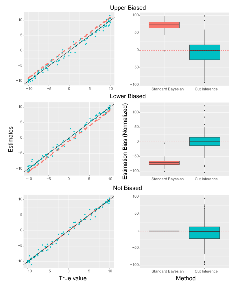
Figure A1: Numerical simulation results of cut inference and standard Bayesian inference under a multiple-module case. Left: scatter plots of the estimates verses true value of parameters. Right: boxplots of the estimation bias after normalization. The estimation bias is normalized according to the standard deviation of the estimates.

We first look at the scenarios when there is a deterministic bias. For the upper bias scenario, estimates of standard Bayesian inference all overestimate the parameter. Similarly, estimates of standard Bayesian inference all underestimate the parameter when there is a lower bias instead. In contrast, the estimates using cut inference evenly distribute around the truth. This indicates that cut inference reduces the estimation bias in this simulation, as the theory in the Section 3.3 indicated.

We now consider the scenario when there is no misspecification. Both standard Bayesian inference and cut inference have correctly estimated the parameter on an average basis with respect to sampling time. Unlike the scenario of misspecification, standard Bayesian inference outperforms cut inference in terms of the variance of the estimation bias. This is expected as the standard Bayesian inference utilizes all available information when the whole model is correctly specified. In contrast, cut inference has prevented the feedback from descendant modules so information is only partially used to infer the parameter.

References

- Andrade et al., (2013) Andrade, J. A. A., Dorea, C. C. Y., and Otiniano, C. E. G. (2013). On the robustness of Bayesian modelling of location and scale structures using heavy-tailed distributions. Communications in Statistics - Theory and Methods, 42(8):1502–1514.
- Arambepola et al., (2020) Arambepola, R., Keddie, S. H., Collins, E. L., Twohig, K. A., Amratia, P., Bertozzi-Villa, A., Chestnutt, E. G., Harris, J., Millar, J., Rozier, J., et al. (2020). Spatiotemporal mapping of malaria prevalence in Madagascar using routine surveillance and health survey data. Scientific reports, 10(1):1–14.
- Arendt et al., (2012) Arendt, P. D., Apley, D. W., and Chen, W. (2012). Quantification of model uncertainty: Calibration, model discrepancy, and identifiability. Journal of Mechanical Design, 134(10). 100908.
- Bhattacharya et al., (2019) Bhattacharya, A., Pati, D., and Yang, Y. (2019). Bayesian fractional posteriors. The Annals of Statistics, 47(1):39 – 66.
- Bissiri et al., (2016) Bissiri, P. G., Holmes, C. C., and Walker, S. G. (2016). A general framework for updating belief distributions. Journal of the Royal Statistical Society: Series B (Statistical Methodology), 78(5):1103–1130.
- Cameron et al., (2021) Cameron, E., Young, A. J., Twohig, K. A., Pothin, E., Bhavnani, D., Dismer, A., Merilien, J. B., Hamre, K., Meyer, P., Le Menach, A., Cohen, J. M., Marseille, S., Lemoine, J. F., Telfort, M.-A., Chang, M. A., Won, K., Knipes, A., Rogier, E., Amratia, P., Weiss, D. J., Gething, P. W., and Battle, K. E. (2021). Mapping the endemicity and seasonality of clinical malaria for intervention targeting in haiti using routine case data. eLife, 10:e62122.
- Carmona and Nicholls, (2020) Carmona, C. and Nicholls, G. (2020). Semi-modular inference: Enhanced learning in multi-modular models by tempering the influence of components. In Chiappa, S. and Calandra, R., editors, Proceedings of the Twenty Third International Conference on Artificial Intelligence and Statistics, volume 108 of Proceedings of Machine Learning Research, pages 4226–4235. PMLR.
- Chakraborty et al., (2022) Chakraborty, A., Nott, D. J., Drovandi, C., Frazier, D. T., and Sisson, S. A. (2022). Modularized Bayesian analyses and cutting feedback in likelihood-free inference.
- Frazier and Nott, (2022) Frazier, D. T. and Nott, D. J. (2022). Cutting feedback and modularized analyses in generalized Bayesian inference.
- Friel and Pettitt, (2008) Friel, N. and Pettitt, A. N. (2008). Marginal likelihood estimation via power posteriors. Journal of the Royal Statistical Society: Series B (Statistical Methodology), 70(3):589–607.
- Holmes and Walker, (2017) Holmes, C. C. and Walker, S. G. (2017). Assigning a value to a power likelihood in a general Bayesian model. Biometrika, 104(2):497–503.
- Jacob et al., (2017) Jacob, P. E., Murray, L. M., Holmes, C. C., and Robert, C. P. (2017). Better together? statistical learning in models made of modules. arXiv preprint arXiv:1708.08719.
- Jacob et al., (2020) Jacob, P. E., O’Leary, J., and Atchadé, Y. F. (2020). Unbiased Markov chain Monte Carlo methods with couplings. Journal of the Royal Statistical Society: Series B (Statistical Methodology), 82(3):543–600.
- Kaplan and Chen, (2012) Kaplan, D. and Chen, J. (2012). A two-step Bayesian approach for propensity score analysis: Simulations and case study. Psychometrika, 77(3):581–609.
- Li et al., (2013) Li, L., Xu, C.-Y., and Engeland, K. (2013). Development and comparison in uncertainty assessment based Bayesian modularization method in hydrological modeling. Journal of Hydrology, 486:384–394.
- Liao and Zigler, (2020) Liao, S. X. and Zigler, C. M. (2020). Uncertainty in the design stage of two-stage Bayesian propensity score analysis. Statistics in Medicine, 39(17):2265–2290.
- Liu et al., (2009) Liu, F., Bayarri, M., Berger, J., et al. (2009). Modularization in Bayesian analysis, with emphasis on analysis of computer models. Bayesian Analysis, 4(1):119–150.
- Liu and Goudie, (2022) Liu, Y. and Goudie, R. J. (2022). Stochastic approximation cut algorithm for inference in modularized Bayesian models. Statistics and Computing, 32(1):1–15.
- Liu and Goudie, (2021) Liu, Y. and Goudie, R. J. B. (2021). Generalized geographically weighted regression model within a modularized Bayesian framework.
- (20) Lunn, D., Best, N., Spiegelhalter, D., Graham, G., and Neuenschwander, B. (2009a). Combining MCMC with ‘sequential’ PKPD modelling. Journal of Pharmacokinetics and Pharmacodynamics, 36(1):19—38.
- (21) Lunn, D., Spiegelhalter, D., Thomas, A., and Best, N. (2009b). The BUGS project: Evolution, critique and future directions. Statistics in Medicine, 28(25):3049–3067.
- McCandless et al., (2010) McCandless, L. C., Douglas, I. J., Evans, S. J., and Smeeth, L. (2010). Cutting feedback in Bayesian regression adjustment for the propensity score. The International Journal of Biostatistics, 6(2).
- Mikkelä et al., (2019) Mikkelä, A., Ranta, J., and Tuominen, P. (2019). A modular Bayesian salmonella source attribution model for sparse data. Risk Analysis, 39(8):1796–1811.
- Miller and Dunson, (2019) Miller, J. W. and Dunson, D. B. (2019). Robust Bayesian inference via coarsening. Journal of the American Statistical Association, 114(527):1113–1125. PMID: 31942084.
- Moss and Rousseau, (2022) Moss, D. and Rousseau, J. (2022). Efficient Bayesian estimation and use of cut posterior in semiparametric hidden Markov models.
- Nicholls et al., (2022) Nicholls, G. K., Lee, J. E., Wu, C.-H., and Carmona, C. U. (2022). Valid belief updates for prequentially additive loss functions arising in semi-modular inference.
- O’Hagan and Pericchi, (2012) O’Hagan, A. and Pericchi, L. (2012). Bayesian heavy-tailed models and conflict resolution: A review. Brazilian Journal of Probability and Statistics, 26(4):372 – 401.
- Plummer, (2015) Plummer, M. (2015). Cuts in Bayesian graphical models. Statistics and Computing, 25(1):37–43.
- Pompe and Jacob, (2021) Pompe, E. and Jacob, P. E. (2021). Asymptotics of cut distributions and robust modular inference using posterior bootstrap.
- Rosenbaum and Rubin, (1983) Rosenbaum, P. R. and Rubin, D. B. (1983). The central role of the propensity score in observational studies for causal effects. Biometrika, 70(1):41–55.
- Rubin, (1990) Rubin, D. B. (1990). Formal mode of statistical inference for causal effects. Journal of Statistical Planning and Inference, 25(3):279–292.
- Rubin, (2008) Rubin, D. B. (2008). For objective causal inference, design trumps analysis. The Annals of Applied Statistics, 2(3):808 – 840.
- Wang and Blei, (2018) Wang, C. and Blei, D. M. (2018). A general method for robust Bayesian modeling. Bayesian Analysis, 13(4):1163 – 1191.
- Yu et al., (2021) Yu, X., Nott, D. J., and Smith, M. S. (2021). Variational inference for cutting feedback in misspecified models.
- Zhang et al., (2003) Zhang, L., Beal, S. L., and Sheiner, L. B. (2003). Simultaneous vs. sequential analysis for population PK/PD data I: best-case performance. Journal of Pharmacokinetics and Pharmacodynamics, 30(6):387–404.
- Zigler, (2016) Zigler, C. M. (2016). The central role of bayes’ theorem for joint estimation of causal effects and propensity scores. The American Statistician, 70(1):47–54. PMID: 27482121.
- Zigler and Dominici, (2014) Zigler, C. M. and Dominici, F. (2014). Uncertainty in propensity score estimation: Bayesian methods for variable selection and model-averaged causal effects. Journal of the American Statistical Association, 109(505):95–107. PMID: 24696528.
- Zigler et al., (2013) Zigler, C. M., Watts, K., Yeh, R. W., Wang, Y., Coull, B. A., and Dominici, F. (2013). Model feedback in Bayesian propensity score estimation. Biometrics, 69(1):263–273.