An Accelerated Variance Reduced Extra-Point Approach to
Finite-Sum VI and Optimization

Abstract

In this paper, we develop stochastic variance reduced algorithms for solving a class of finite-sum monotone VI, where the operator consists of the sum of finitely many monotone VI mappings and the sum of finitely many monotone gradient mappings. We study the gradient complexities of the proposed algorithms under the settings when the sum of VI mappings is either strongly monotone or merely monotone. Furthermore, we consider the case when each of the VI mapping and gradient mapping is only accessible via noisy stochastic estimators and establish the sample gradient complexity. We demonstrate the application of the proposed algorithms for solving finite-sum convex optimization with finite-sum inequality constraints and develop a zeroth-order approach when only noisy and biased samples of objective/constraint function values are available.

Keywords: finite-sum optimization, stochastic gradient method, variational inequality, stochastic zeroth-order method.

1 Introduction

In machine learning research, a common optimization problem is the so-called finite-sum optimization:

$$\min\limits_{x\in{\cal X}}\quad g(x):=\sum\limits_{i=1}^{m}g_{i}(x),$$ (1)

where the objective is the sum of finitely many (convex) loss functions. When the total number of functions is large, it can be costly for a deterministic gradient method to evaluate the gradients of all the functions in each iteration. A conventional way for solving the finite-sum model (1) is through stochastic gradient descent (SGD), where in each iteration only one or a mini-batch of functions are randomly chosen and the corresponding gradients are estimated. While SGD may improve the overall gradient complexity over the deterministic methods, the iteration complexity to obtain an $\epsilon$-solution is only $\mathcal{O}\left(\frac{1}{\epsilon}\right)$ even if each of the function $g_{i}(x)$ is strongly convex and smooth. In order to further improve the gradient and iteration complexity, variance reduced algorithms such as SAG [27], SAGA [6], SVRG [13] have been developed to achieve the gradient complexity $\mathcal{O}\left(\left(m+\frac{L}{\mu}\right)\log\frac{1}{\epsilon}\right)$, assuming each function $g_{i}(x)$ is strongly monotone with modulus $\mu>0$ and gradient Lipschitz continuous with constant $L\geq\mu$. Recently, accelerated variance reduced algorithms such as Katyusha [2] and SSNM [34] are proposed to achieve an even better gradient complexity $\mathcal{O}\left(\left(m+\sqrt{\frac{mL}{\mu}}\right)\log\frac{1}{\epsilon}\right)$, which matches the lower bound established in [15], hence optimal.

A specific branch in machine learning which has received much attention in recent years is training Generative Adversarial Network (GAN) [10]. Different from an optimization model (1), training a GAN can be formulated as a minimax saddle point problem:

$$\min\limits_{x\in{\cal X}}\max\limits_{y\in{\cal Y}}\quad f(x,y).$$ (2)

When $f(\cdot,y)$ is convex for fixed $y\in{\cal Y}$ and $f(x,\cdot)$ is concave for fixed $x\in{\cal X}$ and ${\cal X},{\cal Y}$ are closed convex sets, (2) can be reformulated into a more general variational inequalities (VI) model:

$$\mbox{find $x^{*}$ s.t.}\quad\langle F(x^{*}),x-x^{*}\rangle\geq 0,\quad\forall x\in{\cal Z},$$ (3)

where $F(\cdot)$ is a general monotone vector mapping. Since GAN is known to be very difficult to train and the conventional (stochastic) gradient methods applied for deep learning do not perform well in practice, there has been a surge of interest in developing efficient gradient methods in the context of either saddle point problem or VI [5, 22, 17, 9, 12]. It is also natural to consider the finite-sum VI where $F(x)=\sum\limits_{i=1}^{m}F_{i}(x)$ and develop variance reduced algorithms applying techniques from finite-sum optimization. The authors in [1] incorporated such variance reduced techniques into various VI algorithms and established the gradient complexity $\mathcal{O}\left(m+\frac{\sqrt{m}L}{\epsilon}\right)$ for monotone VI and $\mathcal{O}\left(\left(m+\frac{\sqrt{m}L}{\mu}\right)\log\frac{1}{\epsilon}\right)$ for strongly monotone VI, where each operator $F_{i}(x)$ is (strongly) monotone with modulus $\mu\,(>)\geq 0$ and Lipschitz continuous with $L\geq\mu$. On the other hand, a lower gradient complexity bound has also been established in [32] with $\Omega\left(m+\frac{L}{\epsilon}\right)$ for convex-concave saddle point problem and $\Omega\left(\left(m+\frac{L}{\mu}\right)\log\frac{1}{\epsilon}\right)$ for strongly-convex-strongly-concave saddle point problem. Unlike the accelerated variance reduced algorithms in optimization [2, 34] which have been proven to be optimal, there is still a gap between the upper and lower gradient complexity bounds for finite-sum VI. It remains an open problem to determine where the optimal gradient complexity bound actually lands.

In this paper, we consider an extended class of monotone VI (3) in the finite-sum form, where the operator consists of the sum of finitely many general vector mapping $H_{i}(x)$ and the sum of finitely many gradient mapping $\nabla g_{i}(x)$:

$$F(x)=H(x)+\nabla g(x):=\sum\limits_{i=1}^{m_{1}}H_{i}(x)+\sum\limits_{i=1}^{m_{2}}\nabla g_{i}(x),$$ (4)

where each $H_{i}(\cdot)$ is Lipschitz continuous with $L_{h(i)}$ and $H(\cdot)$ is (strongly) monotone with $\mu\,(>)\geq 0$, and each $\nabla g_{i}(\cdot)$ is Lipschitz continuous with $L_{g(i)}$ and $\nabla g(\cdot)$ is monotone. The pioneering work considering such extended class of monotone VI (4) without the finite-sum structure (i.e. $m_{1}=m_{2}=1$) is [4], where the authors propose a stochastic accelerated mirror-prox method with iteration (sample) complexity

$$\mathcal{O}\left(\sqrt{\frac{L_{g}}{\epsilon}}+\frac{L_{h}}{\epsilon}+\frac{\sigma^{2}}{\epsilon^{2}}\right)$$

for monotone $H(\cdot)$ and $\nabla g(\cdot)$. Note that the subscript $i$ indicating the index in the finite-sum is omitted since $m_{1}=m_{2}=1$. In addition, the authors [4] consider the stochastic setting where both $H(\cdot)$ and $\nabla g(\cdot)$ can only be estimated via an unbiased oracle with bounded variance $\sigma^{2}$. In this paper, we continue along this line of research on the extended class of monotone VI (4) with general $m_{1},m_{2}$ and apply variance reduced techniques to establish accelerated gradient complexity bound. We assume each $H_{i}(\cdot)$ and $\nabla g_{i}(\cdot)$ can only be estimated via a stochastic oracle with bounded variance and bias and give the corresponding sample gradient complexity. We show that the proposed algorithms can be applied to solving finite-sum convex optimization with finite-sum inequality constraints [18] with an improved gradient complexity. Furthermore, the general stochastic setting in this paper makes it possible to apply zeroth-order approach [16] to solve the aforementioned problem with our algorithm, when only biased samples of objective/constraint function values are accessible.

The rest of the paper is organized as follows. In Section 2, we propose a stochastic variance reduced algorithm for the extended class of VI (4) when $H_{i}(\cdot)$ is strongly monotone. In Section 3, we provide an alternative variance reduced method to solve the case when $H_{i}(\cdot)$ is only monotone. In Section 4, we demonstrate the application to solving finite-sum convex optimization with finite-sum inequality constraints. We further extend this application to a more general black-box setting and demonstrate the implementation of our proposed algorithm via a zeroth-order approach. We present numerical results in Section 5 and conclude the paper in Section 6.

2 Variance Reduced Scheme for Finite-Sum Strongly Monotone VI and Finite-Sum Monotone Gradients

In this section, we present our first variance reduced scheme for solving VI (3), where the operator $F(\cdot)$ takes the combined VI/gradient mapping form with finite-sum structure respectively (4). We assume the constraint set ${\cal Z}$ is closed and convex, and the problem is summarized below:

$$\left\{\begin{array}[]{ll}\mbox{find $x^{*}$ s.t.}\quad\langle F(x^{*}),x-x^{*}\rangle\geq 0,\quad\forall x\in{\cal Z},\\ F(x)=H(x)+\nabla g(x):=\sum\limits_{i=1}^{m_{1}}H_{i}(x)+\sum\limits_{i=1}^{m_{2}}\nabla g_{i}(x).\end{array}\right.$$ (7)

We specifically consider the combined finite-sum operator $F(\cdot)$ being strongly monotone in this section, and we shall propose an alternative approach for $F(\cdot)$ being merely monotone in the next section. In particular, we assume $H(\cdot)$ to be strongly monotone with modulus $\mu_{h}>0$, and $\nabla g(\cdot)$ to be monotone. Furthermore, we denote $H(\cdot)=\sum\limits_{i=1}^{m_{1}}H_{i}(\cdot)$, where each $H_{i}(\cdot)$ is Lipschitz continuous with constant $L_{h(i)}$, and denote $g(x)=\sum\limits_{i=1}^{m_{2}}g_{i}(x)$ (therefore $\nabla g(x)=\sum\limits_{i=1}^{m_{2}}\nabla g_{i}(x)$) where each $\nabla g_{i}(x)$ is Lipschitz continuous with constant $L_{g(i)}$. Let us also define the sum of the Lipschitz constants $L_{h}:=\sum\limits_{i=1}^{m_{1}}L_{h(i)}$ and $L_{g}:=\sum\limits_{i=1}^{m_{2}}L_{g(i)}$.

Consider the following update for iteration count $k$:

$$\left\{\begin{array}[]{lcl}\bar{x}^{k}&=&(1-p_{1})x^{k}+p_{1}w^{k}\\ {y^{k}}&=&(1-\alpha-\beta)v^{k}+\alpha x^{k}+\beta\bar{w}^{k}\\ x^{k+0.5}&=&\arg\min\limits_{x\in\mathcal{Z}}\quad\gamma\langle{H^{\prime}}(w^{k})+{\tilde{\nabla}{g^{\prime}}(y^{k})},x-\bar{x}^{k}\rangle+\frac{1}{2}\|x-\bar{x}^{k}\|^{2}\\ x^{k+1}&=&\arg\min\limits_{x\in\mathcal{Z}}\quad\gamma\langle\hat{H^{\prime}}(x^{k+0.5})+{\tilde{\nabla}{g^{\prime}}(y^{k})},x-\bar{x}^{k}\rangle+\frac{1}{2}\|x-\bar{x}^{k}\|^{2}\\ {v^{k+1}}&=&{(1-\alpha-\beta)v^{k}+\alpha x^{k+0.5}+\beta\bar{w}^{k}}\\ w^{k+1}&=&\left\{\begin{array}[]{ll}x^{k+1},&\mbox{with prob. $p_{1}$}\\ w^{k},&\mbox{with prob. $1-p_{1}$}\end{array}\right.\\ \bar{w}^{k+1}&=&\left\{\begin{array}[]{ll}v^{k+1},&\mbox{with prob. $p_{2}$}\\ \bar{w}^{k},&\mbox{with prob. $1-p_{2}$}.\par\end{array}\right.\end{array}\right.$$ (8)

Method (8) is a general stochastic variance reduced scheme for solving (7), and in the rest of the paper we refer to it as Stochastic Accelerated Variance Reduced Extra Point method (SAVREP). We shall make the following remarks. First, the variance reduction techniques are applied to both the general VI operator $H(\cdot)$ and the gradient mapping $\nabla g(\cdot)$, and the resulting update procedure will require using the variance reduced gradient estimator [2, 1], denote by $\hat{H}(\cdot)$ and $\tilde{\nabla}g(\cdot)$, respectively. Second, although the construction of the variance reduced gradient estimator $\hat{H}(\cdot)$ ($\tilde{\nabla}g(\cdot)$) involves sampling from the $m_{1}$ ($m_{2}$) individual operators $H_{i}(\cdot)$ ($\nabla g_{i}(\cdot)$) as we shall see later, we use the term “stochastic” to specifically refer to the fact that the update of SAVREP (8) only accesses the noisy estimations of the individual operators, denote by $H^{\prime}_{i}(\cdot)$ and $\nabla g^{\prime}_{i}(\cdot)$, respectively. This allows the application of zeroth-order approach [16] to problems when the gradients are unavailable and only the function values can be sampled, such as black-box optimization [24, 28, 7, 29] and saddle-point problem [31, 33, 20, 26, 21]. We shall exemplify such application in Section 4. Finally, the multiple-sequence structure of (8) is the key to achieve the overall accelerated variance reduced gradient complexity in terms of both $L_{h}$ and $L_{g}$. While the sequences $\{x^{k+0.5}\},\{x^{k}\}$ in general take the extra-gradient form of update, the sequences $\{w^{k}\},\{\bar{w}^{k}\}$ help maintain the single-loop structure for variance reduction [1]; the sequences $\{y^{k}\},\{v^{k}\}$ help improve the constants related to the gradient mapping, and the sequence $\{\bar{x}^{k}\}$ facilitates the variance reduction for the VI operator $H(\cdot)$. The derivations of gradient complexity and sample complexity involving the analysis of each of these sequences are discussed in Section 2.2, following Section 2.1 where the detailed formulations of the (stochastic) variance reduced gradient estimators and the corresponding assumptions are presented.

2.1 Preliminaries

We first state the assumptions for the stochastic estimators $H^{\prime}_{i}(\cdot)$ $(\nabla g^{\prime}_{i}(\cdot))$ of the individual operators $H_{i}(\cdot)$ $(\nabla g_{i}(\cdot))$ for $i=1,2,...,m_{1}\,(m_{2})$. Denote $\mathbb{E}^{\prime}[\cdot]$ as the expectation taken for these samples and consider the following bias and variance upper bounds:

$$\left\|H_{i}(x)-\mathbb{E}^{\prime}[H^{\prime}_{i}(x)]\right\|\leq\delta_{h},\quad\mathbb{E}^{\prime}\left[\left\|H_{i}^{\prime}(x)-\mathbb{E}^{\prime}\left[H^{\prime}_{i}(x)\right]\right\|^{2}\right]\leq\sigma_{h}^{2},$$ (9)

$${\left\|\nabla g_{i}(x)-\mathbb{E}^{\prime}\left[\nabla g_{i}^{\prime}(x)\right]\right\|\leq\delta_{g},}\quad{\mathbb{E}^{\prime}\left[\left\|\nabla g_{i}^{\prime}(x)-\mathbb{E}^{\prime}\left[\nabla g_{i}^{\prime}(x)\right]\right\|^{2}\right]\leq\sigma_{g}^{2}},$$ (10)

for some $\delta_{h},\sigma_{h}^{2},{\delta_{g},\sigma_{g}^{2}}\geq 0$. In other words, we assume the variance and the bias of these samples are upper bounded by some non-negative constants (therefore they are not necessarily unbiased estimators). Denote $H^{\prime}(x):=\sum\limits_{i=1}^{m_{1}}H^{\prime}_{i}(x)$ (respectively ${\nabla g^{\prime}(x):=\sum\limits_{i=1}^{m_{2}}\nabla g_{i}^{\prime}(x)}$) as the sum of $m_{1}$ (respectively ${m_{2}}$) such independent stochastic oracles. The below bounds follow straightforwardly:

$$\left\|H(x)-\mathbb{E}^{\prime}[H^{\prime}(x)]\right\|\leq m_{1}\delta_{h},\quad\mathbb{E}^{\prime}\left[\left\|H(x)-H^{\prime}(x)\right\|^{2}\right]\leq 2m_{1}\sigma_{h}^{2}+2m_{1}^{2}\delta_{h}^{2},$$ (11)

$${\left\|\nabla g(x)-\mathbb{E}^{\prime}[\nabla g^{\prime}(x)]\right\|\leq m_{2}\delta_{g}},\quad{\mathbb{E}^{\prime}\left[\left\|\nabla g(x)-\nabla g^{\prime}(x)\right\|^{2}\right]\leq 2m_{2}\sigma_{g}^{2}+2m_{2}^{2}\delta_{g}^{2}}.$$ (12)

We next give explicit expressions for the (noiseless) variance reduced gradient estimators at the corresponding iterates given in (8):

$$\hat{{H}}(x^{k+0.5}):={H}(w^{k})+{H}_{\xi_{k}}(x^{k+0.5})-{H}_{\xi_{k}}(w^{k})$$ (13)

$$\tilde{\nabla}{g}(y^{k}):=\nabla{g}(\bar{w}^{k})+\nabla{g_{\zeta_{k}}}(y^{k})-\nabla{g_{\zeta_{k}}}(\bar{w}^{k}).$$ (14)

The above forms follow from the well-established variance reduction literature [2, 1], and the random variables $\xi\,(\zeta)$ take samples from the $m_{1}\,(m_{2})$ individual operators $H_{i}(\cdot)\,(\nabla g_{i}(\cdot))$ with probability distribution taking respective Lipschitz constants $L_{h(i)}\,(L_{g(i)})$ into account. In particular, we have

$$\mbox{Pr}\{\xi=i\}=\frac{L_{h(i)}}{L_{h}}\,:=q_{i},\,\,i=1,2,...,m_{1},\quad\mbox{Pr}\{\zeta=i\}=\frac{L_{g(i)}}{L_{g}}\,:=\pi_{i},\,\,i=1,2,...,m_{2}.$$

The stochastic oracles are then given by $H_{\xi}(\cdot):=\frac{1}{q_{i}}H_{i}(\cdot)$ and $\nabla g_{\zeta}(\cdot)=\frac{1}{\pi_{i}}\nabla g_{i}(\cdot)$.

However, note that in the update (8), only the noisy variance reduced gradient operators $\hat{H}^{\prime}(x^{k+0.5})$ $(\tilde{\nabla}g^{\prime}(y^{k}))$ are accessed, which are defined by:

$$\hat{{H^{\prime}}}(x^{k+0.5}):={H^{\prime}}(w^{k})+{H}_{\xi_{k}}^{\prime}(x^{k+0.5})-{H}_{\xi_{k}}^{\prime}(w^{k})$$

$$\tilde{\nabla}{g^{\prime}}(y^{k}):=\nabla{g^{\prime}}(\bar{w}^{k})+\nabla{g_{\zeta_{k}}^{\prime}}(y^{k})-\nabla{g_{\zeta_{k}}^{\prime}}(\bar{w}^{k}),$$

where $H_{\xi}^{\prime}(\cdot):=\frac{1}{q_{i}}H_{i}^{\prime}(\cdot)$ and $\nabla g_{\zeta}^{\prime}(\cdot)=\frac{1}{\pi_{i}}\nabla g_{i}^{\prime}(\cdot)$. To save the computational costs, we can reuse the noisy samples estimated at the same iterate within each iteration. For example, after sampling $H^{\prime}(w^{k})$ in the update of $x^{k+0.5}$, we could reuse the oracles for $H_{\xi_{k}}^{\prime}(w^{k})$ and $H^{\prime}(w^{k})$ in constructing $\hat{H}^{\prime}(x^{k+0.5})$.

Finally, to simplify the notations in the following analysis, denote the expressions of conditional expectations taken for different random variables:

$$\mathbb{E}_{k_{1}}[\cdot]:=\mathbb{E}_{\xi_{k}}[\cdot|x^{k},w^{k}],\quad\mathbb{E}_{k_{2}}[\cdot]:=\mathbb{E}_{\zeta_{k}}[\cdot|x^{k},\bar{w}^{k},v^{k}],$$ (15)

$$\mathbb{E}_{k_{1}+}[\cdot]:=\mathbb{E}_{\xi_{k}}[\cdot|x^{k+1},w^{k}],\quad\mathbb{E}_{k_{2}+}[\cdot]:=\mathbb{E}_{\zeta_{k}}[\cdot|\bar{w}^{k},v^{k+1}].$$ (16)

2.2 Gradient complexity analysis

The overall analysis for gradient complexity of the proposed SAVREP (8) can be largely divided into three parts. In the first part, the stochastic gradient mapping $\tilde{\nabla}g^{\prime}(y^{k})$ is viewed as a constant vector mapping, and we establish the relation among the sequences $\{\bar{x}^{k}\}$, $\{x^{k+0.5}\}$, $\{x^{k}\}$, $\{w^{k}\}$, which are related to the general VI mapping $H(\cdot)$. In the second part, we turn to focus on the sequences $\{y^{k}\}$, $\{v^{k}\}$, $\{\bar{w}^{k}\}$, and establish their relation in terms of the function value $g(\cdot)$. Finally, the results in the previous two parts are combined to show the per-iteration convergence in terms of a potential function. By selecting the parameters carefully, we derive the resulting gradient complexity for obtaining an $\epsilon$-solution $\mathbb{E}\left[\|x^{k}-x^{*}\|^{2}\right]\leq\epsilon$, together with the corresponding stochastic errors. The lemma below summarizes the results from the first part of the analysis.

Lemma 2.1.

For the iterates generated by (8), define the following stochastic error terms:

$$\varepsilon_{x}:=\|H_{\xi}(x)-H_{\xi}^{\prime}(x)\|,\quad\bar{\varepsilon}_{x}:=\|H(x)-H^{\prime}(x)\|.$$

Then, the following inequality holds for any $x\in{\cal Z}$ and $k=0,1,2,...$

$$\mathbb{E}_{k_{1}}\left[\gamma\langle H(x)+\tilde{\nabla}{g^{\prime}}(y^{k}),x^{k+0.5}-x\rangle\right]$$

$$\leq \frac{1}{2}\mathbb{E}_{k_{1}}\left[(1-p_{1}-{\frac{1}{2}}\gamma\mu_{h})\|x^{k}-x\|^{2}+p_{1}\|w^{k}-x\|^{2}-\|x^{k+1}-x\|^{2}\right]$$

$$-\frac{1}{2}\left(p_{1}-{2}\gamma^{2}L_{h}^{2}\right)\mathbb{E}_{k_{1}}\left[\|x^{k+0.5}-w^{k}\|^{2}\right]-\frac{1}{2}\left(1-p_{1}-\gamma\mu_{h}\right)\mathbb{E}_{k_{1}}\left[\|x^{k+0.5}-x^{k}\|^{2}\right]$$

$${+\frac{\gamma\bar{\varepsilon}_{x^{k+0.5}}^{2}}{2\mu_{h}}+\gamma^{2}\mathbb{E}_{k_{1}}\left[(\varepsilon_{x^{k+0.5}}+\varepsilon_{w^{k}})^{2}\right]}.$$

Proof.

See Appendix A.1. ∎

In Lemma 2.1, we define two stochastic error terms, $\varepsilon_{x}$ and $\bar{\varepsilon}_{x}$, which are due to the noisy samples of $H_{i}(\cdot)$. We can first bound the squared stochastic error $\bar{\varepsilon}_{x}^{2}$ for the total operator $H(\cdot)$ with our assumption in (11):

$$\mathbb{E}^{\prime}[\bar{\varepsilon}_{x}^{2}]\leq 2m_{1}\sigma_{h}^{2}+2m_{1}^{2}\delta_{h}^{2}.$$

On the other hand, the error $\varepsilon_{x}$ involves a random variable $\xi$ sampled from $i=1,...,m_{1}$. Since

$$\mathbb{E}_{\xi}\left[\varepsilon_{x}^{2}\right]=\sum\limits_{i=1}^{m_{1}}q_{i}\cdot\frac{1}{q_{i}^{2}}\|H_{i}^{\prime}(x)-H_{i}(x)\|^{2}=\sum\limits_{i=1}^{m_{1}}\frac{1}{q_{i}}\|H_{i}^{\prime}(x)-H_{i}(x)\|^{2},$$

we have

$$\mathbb{E}^{\prime}\left[\varepsilon_{x}^{2}\right]=\mathbb{E}^{\prime}\left[\mathbb{E}_{\xi}\left[\varepsilon_{x}^{2}\right]\right] \leq \sum\limits_{i=1}^{m_{1}}\frac{2}{q_{i}}\mathbb{E}^{\prime}\left[\left\|H_{i}^{\prime}(x)-\mathbb{E}^{\prime}\left[H_{i}^{\prime}(x)\right]\right\|^{2}+\left\|\mathbb{E}^{\prime}\left[H_{i}^{\prime}(x)\right]-H_{i}(x)\right\|^{2}\right]$$ (17)

$$\leq 2(\sigma_{h}^{2}+\delta_{h}^{2})\cdot\sum\limits_{i=1}^{m_{1}}\frac{1}{q_{i}}=2L_{h}\cdot(\sigma_{h}^{2}+\delta_{h}^{2})\cdot\sum\limits_{i=1}^{m_{1}}\frac{1}{L_{h(i)}}:=\tilde{\sigma}_{h}^{2}.$$

Now we shall proceed to present the results in the second part of the analysis, summarized in the next lemma.

Lemma 2.2.

For the iterates generated by (8), define the following stochastic error terms:

$$\rho_{x}:=\|\nabla g_{\zeta}(x)-\nabla g_{\zeta}^{\prime}(x)\|,\quad\bar{\rho}_{x}:=\|\nabla g(x)-\nabla g^{\prime}(x)\|.$$

With the condition $1-\alpha-\beta\geq 0$, the following inequality holds for any $x\in{\cal Z}$ and $k=0,1,2,...$

$$\mathbb{E}_{k_{2}}\left[g(v^{k+1})-g(x)\right] \leq \mathbb{E}_{k_{2}}\left[(1-\alpha-\beta)\left(g(v^{k})-g(x)\right)+\beta\left(g(\bar{w}^{k})-g(x)\right)\right]$$

$$+\mathbb{E}_{k_{2}}\left[\alpha\langle\tilde{\nabla}g^{\prime}(y^{k}),x^{k+0.5}-x\rangle\right]+{\left(\frac{\alpha^{2}L_{g}}{2}+\frac{\alpha^{2}L_{g}}{2\beta}+\frac{\alpha\mu_{h}}{8}\right)}\mathbb{E}_{k_{2}}\left[\|x^{k+0.5}-x^{k}\|^{2}\right]$$

$$+{\frac{\alpha\mu_{h}}{8}\mathbb{E}_{k_{2}}\left[\|x^{k}-x\|^{2}\right]+\frac{8\alpha}{\mu_{h}}\mathbb{E}_{k_{2}}[\bar{\rho}_{\bar{w}^{k}}^{2}]+\frac{8\alpha}{\mu_{h}}\mathbb{E}_{k_{2}}\left[(\rho_{\bar{w}^{k}}+\rho_{y^{k}})^{2}\right]}.$$

Proof.

See Appendix A.2. ∎

Similarly, we define the two stochastic error terms in Lemma 2.2, $\rho_{x}$ and $\bar{\rho}_{x}$, which are due to the noisy samples of the gradient mapping $\nabla g_{i}(\cdot)$. The bound for $\bar{\rho}_{x}^{2}$ follows directly from (12):

$$\mathbb{E}^{\prime}[\bar{\rho}_{x}^{2}]\leq 2m_{2}\sigma_{g}^{2}+2m_{2}^{2}\delta_{g}^{2},$$

whereas the bound for $\rho_{x}^{2}$ can be derived as follows

$$\mathbb{E}^{\prime}\left[\mathbb{E}_{\zeta}[\rho_{x}^{2}]\right]$$ (18)

$$= \mathbb{E}^{\prime}\left[\mathbb{E}_{\zeta}\left[\|\nabla g_{\zeta}(x)-\nabla g_{\zeta}^{\prime}(x)\|^{2}\right]\right]$$

$$= \mathbb{E}^{\prime}\left[\sum\limits_{i=1}^{m_{2}}\pi_{i}\cdot\frac{1}{\pi_{i}^{2}}\|\nabla g_{i}(x)-\nabla g^{\prime}_{i}(x)\|^{2}\right]$$

$$\leq \sum\limits_{i=1}^{m_{2}}\frac{2}{\pi_{i}}\mathbb{E}^{\prime}\left[\left\|\nabla{g}_{i}(x)-\mathbb{E}^{\prime}\left[\nabla{g}_{i}^{\prime}(x)\right]\right\|^{2}+\left\|\mathbb{E}^{\prime}\left[\nabla{g}_{i}^{\prime}(x)\right]-\nabla{g}_{i}^{\prime}(x)\right\|^{2}\right]$$

$$\leq 2(\sigma_{g}^{2}+\delta_{g}^{2})\cdot\sum\limits_{i=1}^{m_{2}}\frac{1}{\pi_{i}}=2L_{g}\cdot(\sigma_{g}^{2}+\delta_{g}^{2})\cdot\sum\limits_{i=1}^{m_{2}}\frac{1}{L_{g(i)}}:=\tilde{\sigma}_{g}^{2}.$$

The last part of the analysis will combine the results from Lemma 2.1 and Lemma 2.2 and establish the overall per-iteration convergence in terms of a potential function. Let us first define the following function, which serves as an important component in our potential function:

$$Q(x^{\prime};x):=\langle H(x),x^{\prime}-x\rangle+g(x^{\prime})-g(x).$$

In particular, we will use the function $Q(x^{\prime};x^{*})$ with $x^{\prime}$ being the iterates generated by SAVREP (8). The following properties show that $Q(x^{\prime};x^{*})$ is nonnegative for any $x^{\prime}\in{\cal Z}$ and is upper-bounded in terms of $x^{\prime}$:

$$Q(x^{\prime};x^{*})=\langle H(x^{*}),x^{\prime}-x^{*}\rangle+g(x^{\prime})-g(x^{*})\geq\langle H(x^{*})+\nabla g(x^{*}),x^{\prime}-x^{*}\rangle\geq 0.$$ (19)

and

$$Q(x^{\prime};x^{*}) = \langle H(x^{*}),x^{\prime}-x^{*}\rangle+g(x^{\prime})-g(x^{*})$$

$$\leq \langle H(x^{\prime}),x^{\prime}-x^{*}\rangle-\mu_{h}\|x^{\prime}-x^{*}\|^{2}+g(x^{\prime})-g(x^{*})$$

$$\leq \langle H(x^{\prime})+\nabla g(x^{\prime}),x^{\prime}-x^{*}\rangle-\mu_{h}\|x^{\prime}-x^{*}\|^{2}\leq\frac{1}{4\mu_{h}}\left\|H(x^{\prime})+\nabla g(x^{\prime})\right\|^{2}.$$

Now we are ready to show the per-iteration convergence for (8):

Theorem 2.3.

For the iterates generated by (8), define the following constants:

$$\Delta_{h}:=\frac{\alpha}{\mu_{h}}(m_{1}\sigma_{h}^{2}+m_{1}^{2}\delta_{h}^{2})+2\alpha\gamma\tilde{\sigma}_{h}^{2},\quad\Delta_{g}:=\frac{16\alpha}{\mu_{h}}(m_{2}\sigma_{g}^{2}+m_{2}^{2}\delta_{g}^{2})+\frac{16\alpha}{\mu_{h}}\tilde{\sigma}_{g}^{2}.$$

Then, the following inequality holds for $k=0,1,2,...$

$$\mathbb{E}\left[(1-\phi p_{2})Q(v^{k+1};x^{*})+\phi Q(\bar{w}^{k+1};x^{*})\right]+\frac{\alpha}{2\gamma}\mathbb{E}\left[(1-p_{1})\|x^{k+1}-x^{*}\|^{2}+\|w^{k+1}-x^{*}\|^{2}\right]$$ (20)

$$\leq \mathbb{E}\left[(1-\alpha-\beta)Q(v^{k};x^{*})+(\beta+\phi(1-p_{2}))Q(\bar{w}^{k};x^{*})\right]$$

$$+\left(1-\frac{\gamma\mu_{h}}{12}\right)\frac{\alpha}{2\gamma}\mathbb{E}\left[\left(1-p_{1}\right)\|x^{k}-x^{*}\|^{2}+\|w^{k}-x^{*}\|^{2}\right]+\Delta_{h}+\Delta_{g}.$$

Proof.

See Appendix A.3. ∎

Theorem 2.3 establishes the relation for the iterates generated by (8), with additional stochastic errors $\Delta_{h}$, $\Delta_{g}$ due to the noisy samples taken for $H_{i}(\cdot)$ and $\nabla g_{i}(\cdot)$. To further derive the gradient complexity and the overall stochastic errors, we are left with specifying the parameters $\alpha,\beta,\gamma,\phi,p_{1},p_{2}$. Note that in deriving (20), we have imposed the constraints (92) on some of the parameters (see Appendix A.3), together with the condition $1-\alpha-\beta\geq 0$ in Lemma 2.2, which should be honored during the parameter selection process. We summarize the gradient complexity results in the next proposition:

Proposition 2.4.

In view of Theorem 2.3, by specifying the following parameters:

$$\gamma=\frac{1}{4}\min\left(\frac{\sqrt{p_{1}}}{L_{h}},\sqrt{\frac{p_{2}}{L_{g}\mu_{h}}},\frac{p_{1}}{\mu_{h}}\right),\quad\alpha=\frac{1}{12}\min\left(\sqrt{\frac{\mu_{h}}{L_{g}p_{2}}},1\right),\quad\beta=\frac{1}{2},$$

and

$$\phi=\frac{(1+\alpha)m_{2}}{2},\quad p_{1}=\frac{1}{m_{1}},\quad p_{2}=\frac{1}{m_{2}},$$

the gradient complexity for reducing the deterministic errors to some $\epsilon>0$ is

$$\mathcal{O}\left(\left(m_{1}+m_{2}+\sqrt{\frac{L_{g}m_{2}}{\mu_{h}}}+\frac{L_{h}\sqrt{m_{1}}}{\mu_{h}}\right)\log\frac{d_{0}}{\epsilon}\right),$$ (21)

where

$$d_{0}:=\frac{\gamma}{\alpha\mu_{h}}\left\|H(x^{0})+\nabla g(x^{0})\right\|^{2}+2\|x^{0}-x^{*}\|^{2}.$$

In addition, the overall stochastic error after reducing the deterministic error to $\epsilon$ is of the order

$$\mathcal{O}\left(\left(m_{1}+m_{2}+\sqrt{\frac{L_{g}m_{2}}{\mu_{h}}}+\frac{L_{h}\sqrt{m_{1}}}{\mu_{h}}\right)\cdot\frac{\gamma}{\alpha}\cdot(\Delta_{h}{+\Delta_{g}})\right).$$ (22)

Proof.

See Appendix A.4. ∎

A few remarks are in order to interpret the results in Proposition 2.4.

Remark 2.5.

Under the noiseless case where $H_{i}(\cdot)$ and $\nabla g_{i}(\cdot)$ can be computed exactly ($\delta_{h}=\sigma_{h}=\delta_{g}=\sigma_{g}=0$), (21) gives the iteration complexity before reaching either $\|x^{k}-x^{*}\|^{2}\leq\epsilon$ or $\|w^{k}-w^{*}\|^{2}\leq\epsilon$. Since in each iteration the full operator $H(\cdot)$ ($\nabla g(\cdot)$) is estimated at $w^{k}/\bar{w}^{k}$, which in expectation only updates every $m_{1}$ ($m_{2}$) iterations, the expected cost for estimating an individual operator $H_{i}(\cdot)$ ($\nabla g_{i}(\cdot)$) is constant. Therefore, (21) is also the gradient complexity for obtaining the $\epsilon$-solution.

For a general strongly monotone VI, [1] has established the $\mathcal{O}\left(\left(m_{1}+\frac{L_{h}\sqrt{m_{1}}}{\mu_{h}}\right)\log\frac{1}{\epsilon}\right)$ gradient complexity, while for strongly convex optimization [2, 34] the gradient complexity
$\mathcal{O}\left(\left(m_{2}+\sqrt{\frac{L_{g}m_{2}}{\mu_{g}}}\right)\log\frac{1}{\epsilon}\right)$ has been established. While the former gradient complexity has not been shown tight for VI, Proposition 2.4 implies that it is indeed possible to improve upon the previous results and reflect the accelerated complexity from optimization, when the VI is of the specific form (7).

Remark 2.6.

Under the noisy case when the operators can only be estimated inexactly, the stochastic error $\Delta_{h}+\Delta_{g}$ will be carried throughout the iterations. Provided that the total number of iterations is in the order (21), the overall error is given by $\epsilon+\Delta_{T}$, where we refer to $\epsilon$ as the “deterministic error”. The order of the overall “stochastic error” $\Delta_{T}$, is then given by (22). Through standard techniques such as increasing the sample size for $H^{\prime}_{i}(\cdot)$ ($\nabla g^{\prime}_{i}(\cdot)$), the overall stochastic error $\Delta_{T}$ can be further reduced to $\mathcal{O}(\epsilon)$.

3 Variance Reduced Scheme for Finite-Sum Monotone VI and Finite-Sum Monotone Gradients

In this section, we develop a new algorithm for the same finite-sum monotone VI in the form (7), but now we only assume $H(\cdot)$ to be monotone instead of strongly monotone, i.e. $\mu_{h}=0$ (the monotone assumption for $\nabla g(\cdot)$ remains). The loss of strong monotonicity assumption therefore requires a different design of update procedure and analysis from the previous section, as we shall present shortly later. Same as in the previous section, we define $H(\cdot)=\sum\limits_{i=1}^{m_{1}}H_{i}(\cdot)$ where each $H_{i}(\cdot)$ is Lipschitz continuous with constant $L_{h(i)}$, and $g(x)=\sum\limits_{i=1}^{m_{2}}g_{i}(x)$ is sum of Lipschitz continuous gradient mappings, each with Lipschitz constant $L_{g(i)}$. The rest of the setups in Section 2.1 also apply, and we shall only supplement with some specific changes in the analysis that follows.

Consider the following update for iteration count $k$:

$$\left\{\begin{array}[]{lcl}\bar{x}^{k}&=&(1-p_{1})x^{k}+p_{1}w^{k}\\ {y^{k}}&=&(1-\alpha_{k}-\beta_{k})v^{k}+\alpha_{k}x^{k}+\beta_{k}\bar{w}^{k}\\ x^{k+0.5}&=&\arg\min\limits_{x\in\mathcal{Z}}\quad\gamma_{k}\langle H^{\prime}(w^{k})+{\tilde{\nabla}g^{\prime}(y^{k})},x-\bar{x}^{k}\rangle+\frac{1}{2}\|x-\bar{x}^{k}\|^{2}\\ x^{k+1}&=&\arg\min\limits_{x\in\mathcal{Z}}\quad\gamma_{k}\langle\hat{H}^{\prime}(x^{k+0.5})+{\tilde{\nabla}g^{\prime}(y^{k})},x-\bar{x}^{k}\rangle+\frac{1}{2}\|x-\bar{x}^{k}\|^{2}\\ {v^{k+1}}&=&{(1-\alpha_{k}-\beta_{k})v^{k}+\alpha_{k}x^{k+0.5}+\beta_{k}\bar{w}^{k}}\\ w^{k+1}&=&\left\{\begin{array}[]{ll}x^{k+1},&\mbox{with prob. $p_{1}$}\\ w^{k},&\mbox{with prob. $1-p_{1}$}\par\end{array}\right.\\ \bar{w}^{k+1}&=&\left\{\begin{array}[]{ll}\frac{1}{m_{2}}\sum_{i=k+2-m_{2}}^{k+1}v^{i},&\mbox{$m_{2}|(k+1)$}\\ \bar{w}^{k},&\mbox{otherwise}.\end{array}\right.\end{array}\right.$$ (23)

There are two main differences between the update (23) presented above and the update (8) in the previous section. First, while (8) simply updates $\bar{w}^{k}$ with probability $p_{2}=\frac{1}{m_{2}}$ in each iteration, (23) has a double-loop structure, which updates $\bar{w}^{k}$ once every $m_{2}$ iterations. In other words, the full gradient $\nabla g(\bar{w}^{k})$ is only estimated at the beginning of each outer-loop, and such gradient is used to obtain the variance reduced gradient $\tilde{\nabla}g(y^{k})$ within each inner-loop. Although in [14] single-loop variants of Katyusha and SVRG are developed for strongly convex finite-sum optimization, there are no single-loop variants yet for the convex case as far as our knowledge goes. Therefore, this double-loop structure given in (23) also turns out to be critical in the monotone VI setting. Second, instead of using constant parameters as in (8), the update (23) uses parameters $\alpha_{k},\beta_{k},\gamma_{k}$ that depend on iteration number $k$. This change is again reasonable to make given our (non-strongly) monotone assumption in this section, and it is also consistent with the literature of finite-sum algorithms under the non-strongly convex setting. For example, Katyusha also has parameters depending on epochs. We shall refer to the update (23) as SAVREP-m (SAVREP for monotone VI) in the rest of the paper.

3.1 Gradient complexity analysis

In order to establish a theoretical guarantee for the gradient complexity, we make two additional assumptions compared to the analysis of SAVREP. In particular, we assume that the stochastic estimators $H^{\prime}_{i}(x)$ and $\nabla g^{\prime}_{i}(x)$ are unbiased, and the constraint set ${\cal Z}$ is bounded, as summarized below.

Assumption 3.1.

The stochastic estimators $H_{i}^{\prime}(x)$ and $\nabla g_{i}^{\prime}(x)$ are both unbiased, i.e. $\delta_{h}=\delta_{g}=0$ in (9)-(10).

Assumption 3.2.

The diameter of the constraint set ${\cal Z}$ is $\Omega_{\cal Z}$, i.e.

$$\sup_{x,y\in{\cal Z}}\|x-y\|=\Omega_{\cal Z}.$$ (24)

The gradient complexity analysis of SAVREP-m (23) consists of two major steps. The first step is to derive the per-iteration relation among iterates and establish a result similar to Theorem 2.3. In the first step, we only consider the iterations from $k$ to $k+1$, which is within a single inner-loop in the update (23) with $\bar{w}^{k}$ remaining unchanged. In the second step, we derive the relation among iterates after one outer-loop, where the iterations proceed from $sm_{2}$ to $(s+1)m_{2}$. This step specifically establishes an inequality relating $\bar{w}^{(s+1)m_{2}}$ and $\bar{w}^{sm_{2}}$, which eventually guarantees the convergence of the iterate $\bar{w}^{k}$ as long as the parameters are chosen to satisfy certain conditions.

The results derived from the first step is presented in the next lemma:

Lemma 3.3.

For the iterates generated by (23), assume the following condition holds for all $k\geq 0$:

$$\left\{\begin{array}[]{ll}p_{1}-2\gamma_{k}^{2}L_{h}^{2}\geq 0,\\ q-p_{1}-\alpha_{k}\gamma_{k}L_{g}-\frac{\alpha_{k}\gamma_{k}L_{g}}{\beta_{k}}\geq 0,\\ {1-\alpha_{k}-\beta_{k}\geq 0}\end{array}\right.$$ (25)

where $0<q<1$ is a constant independent of the problem and algorithm parameters. Then we have:

$$\mathbb{E}\left[Q(v^{k+1};x)\right]+\frac{\alpha_{k}}{2\gamma_{k}}\mathbb{E}\left[(1-p_{1})\|x^{k+1}-x\|^{2}+\|w^{k+1}-x\|^{2}\right]$$

$$\leq \mathbb{E}\left[(1-\alpha_{k}-\beta_{k})Q(v^{k};x)+\beta_{k}Q(\bar{w}^{k};x)\right]+\frac{\alpha_{k}}{2\gamma_{k}}\mathbb{E}\left[\left(1-p_{1}\right)\|x^{k}-x\|^{2}+\|w^{k}-x\|^{2}\right]+\alpha_{k}\gamma_{k}\Delta$$

where $\Delta$ is the stochastic error defined as:

$$\Delta=2\tilde{\sigma}_{h}^{2}+\frac{1}{(1-q)}(2m_{2}\sigma_{g}^{2}+4\tilde{\sigma}_{g}^{2})=O\left(\sigma_{h}^{2}L_{h}\sum\limits_{i=1}^{m_{1}}\frac{1}{L_{h(i)}}+\sigma_{g}^{2}L_{g}\sum\limits_{i=1}^{m_{2}}\frac{1}{L_{g(i)}}\right).$$

Proof.

See Appendix A.5. ∎

Note that while Lemma 3.3 establishes the relation of iterates between iteration $k$ and $k+1$, $\bar{w}^{k}$ remains unchanged (unless $m_{2}|k+1$). Since $\bar{w}^{k}$ plays the central role in the convergence under the monotone case, we have to extend the result in (3.3) to iterations between $sm_{2}$ and $(s+1)m_{2}$, where $s$ denotes the number of outer-loops (or epochs). In particular, we assume that the parameters $\alpha_{k},\beta_{k},\gamma_{k}$ are also unchanged within each interval of updating $\bar{w}^{k}$, i.e.  $\alpha_{sm_{2}}=\alpha_{sm_{2}+1}=\cdots=\alpha_{(s+1)m_{2}-1}$, $\beta_{sm_{2}}=\beta_{sm_{2}+1}=\cdots=\beta_{(s+1)m_{2}-1}$, and $\gamma_{sm_{2}}=\gamma_{sm_{2}+1}=\cdots=\gamma_{(s+1)m_{2}-1}$. Then, by summing up inequality (3.3) from $k=sm_{2}$ to $k=(s+1)m_{2}-1$, we get

$$\mathbb{E}\left[Q(v^{(s+1)m_{2}};x)+(\alpha_{sm_{2}}+\beta_{sm_{2}})\sum_{k=sm_{2}+1}^{(s+1)m_{2}-1}Q(v^{k};x)\right]$$ (27)

$$+\frac{\alpha_{sm_{2}}}{2\gamma_{sm_{2}}}\mathbb{E}\left[(1-p_{1})\|x^{(s+1)m_{2}}-x\|^{2}+\|w^{(s+1)m_{2}}-x\|^{2}\right]$$

$$\leq (1-\alpha_{sm_{2}}-\beta_{sm_{2}})\mathbb{E}[Q(v^{sm_{2}};x)]+\beta_{sm_{2}}m_{2}\mathbb{E}[Q(\bar{w}^{sm_{2}};x)]$$

$$+\frac{\alpha_{sm_{2}}}{2\gamma_{sm_{2}}}\mathbb{E}\left[(1-p_{1})\|x^{sm_{2}}-x\|^{2}+\|w^{sm_{2}}-x\|^{2}\right]+m_{2}\alpha_{sm_{2}}\gamma_{sm_{2}}\Delta.$$

Since $Q(x^{\prime};x):=\langle H(x),x^{\prime}-x\rangle+g(x^{\prime})-g(x)$ and $g$ is convex, $Q(\cdot;x)$ is convex. By using the definition $\bar{w}^{sm_{2}}=\frac{1}{m_{2}}\sum_{i=(s-1)m_{2}+1}^{sm_{2}}v^{i}$ and the convexity of $Q(\cdot;x)$, we have $\sum_{k=(s-1)m_{2}+1}^{sm_{2}}Q(v^{k};x)\geq m_{2}Q(\bar{w}^{sm_{2}};x)$. Then,

$$\mathbb{E}\left[Q(v^{(s+1)m_{2}};x)+(\alpha_{sm_{2}}+\beta_{sm_{2}})\sum_{k=sm_{2}+1}^{(s+1)m_{2}-1}Q(v^{k};x)\right]$$ (28)

$$+\frac{\alpha_{sm_{2}}}{2\gamma_{sm_{2}}}\mathbb{E}[(1-p_{1})\|x^{(s+1)m_{2}}-x\|^{2}+\|w^{(s+1)m_{2}}-x\|^{2}]$$

$$\leq (1-\alpha_{sm_{2}})\mathbb{E}[Q(v^{sm_{2}};x)]+\beta_{sm_{2}}\mathbb{E}\left[\sum_{k=(s-1)m_{2}+1}^{sm_{2}-1}Q(v^{k};x)\right]$$

$$+\frac{\alpha_{sm_{2}}}{2\gamma_{sm_{2}}}\mathbb{E}[(1-p_{1})\|x^{sm_{2}}-x\|^{2}+\|w^{sm_{2}}-x\|^{2}]+m_{2}\alpha_{sm_{2}}\gamma_{sm_{2}}\Delta.$$

Let us define

$$\Gamma_{s}=\left\{\begin{array}[]{lr}1,&\text{ when }s=0\\ (1-\alpha_{(s-1)m_{2}})\Gamma_{s-1},&\text{ when }s>0\end{array}\right.$$

and

$$V(x^{\prime},w;x)=(1-p_{1})\|x^{\prime}-x\|^{2}+\|w-x\|^{2}.$$

Then, by dividing $\Gamma_{s+1}$ on both sides of 28, we have

$$\mathbb{E}\left[\frac{1}{\Gamma_{s+1}}Q(v^{(s+1)m_{2}};x)+\frac{\alpha_{sm_{2}}+\beta_{sm_{2}}}{\Gamma_{s+1}}\sum_{k=sm_{2}+1}^{(s+1)m_{2}-1}Q(v^{k};x)\right]$$ (29)

$$\leq \frac{1}{\Gamma_{s}}\mathbb{E}[Q(v^{sm_{2}};x)]+\frac{\beta_{sm_{2}}}{\Gamma_{s+1}}\mathbb{E}\left[\sum_{k=(s-1)m_{2}+1}^{sm_{2}-1}Q(v^{k};x)\right]$$

$$+\frac{\alpha_{sm_{2}}}{2\gamma_{sm_{2}}\Gamma_{s+1}}\mathbb{E}\left[V(x^{sm_{2}},w^{sm_{2}};x)-V(x^{(s+1)m_{2}},w^{(s+1)m_{2}};x)\right]$$

$$+\frac{m_{2}\alpha_{sm_{2}}\gamma_{sm_{2}}}{\Gamma_{s+1}}\Delta.$$

Since for any solution $x^{*}$ we have $Q(x;x^{*})\geq 0$ for all $x\in{\cal Z}$ (c.f. (19)), by taking $x=x^{*}$ in (29) with the condition on the parameters:

$$\frac{\beta_{sm_{2}}}{\Gamma_{s+1}}\leq\frac{\alpha_{(s-1)m_{2}}+\beta_{(s-1)m_{2}}}{\Gamma_{s}},$$ (30)

we can rewrite (29) into:

$$\mathbb{E}\left[\frac{1}{\Gamma_{s+1}}Q(v^{(s+1)m_{2}};x^{*})+\frac{\alpha_{sm_{2}}+\beta_{sm_{2}}}{\Gamma_{s+1}}\sum_{k=sm_{2}+1}^{(s+1)m_{2}-1}Q(v^{k};x^{*})\right]$$ (31)

$$\leq \frac{1}{\Gamma_{s}}\mathbb{E}[Q(v^{sm_{2}};x^{*})]+\frac{\alpha_{(s-1)m_{2}}+\beta_{(s-1)m_{2}}}{\Gamma_{s}}\mathbb{E}\left[\sum_{k=(s-1)m_{2}+1}^{sm_{2}-1}Q(v^{k};x^{*})\right]$$

$$+\frac{\alpha_{sm_{2}}}{2\gamma_{sm_{2}}\Gamma_{s+1}}\mathbb{E}\left[V(x^{sm_{2}},w^{sm_{2}};x^{*})-V(x^{(s+1)m_{2}},w^{(s+1)m_{2}};x^{*})\right]$$

$$+\frac{m_{2}\alpha_{sm_{2}}\gamma_{sm_{2}}}{\Gamma_{s+1}}\Delta.$$

Now, define

$$B_{s}=\frac{\alpha_{sm_{2}}}{2\gamma_{sm_{2}}\Gamma_{s+1}}$$

and assume the next condition holds for $s=1,...,S-1$:

$$B_{s-1}\leq B_{s}.$$ (32)

Then we can obtain the next inequalities by summing up (31) for $s=1,...,S-1$:

$$\frac{m_{2}\beta_{(S-1)m_{2}}}{\Gamma_{S}}\mathbb{E}\left[Q(\bar{w}^{Sm_{2}};x^{*})\right]$$

$$\leq \mathbb{E}\left[\frac{1}{\Gamma_{S}}Q(v^{Sm_{2}};x^{*})+\frac{\alpha_{(S-1)m_{2}}+\beta_{(S-1)m_{2}}}{\Gamma_{S}}\sum_{k=(S-1)m_{2}+1}^{Sm_{2}-1}Q(v^{k};x^{*})\right]$$

$$\leq \frac{1}{\Gamma_{1}}\mathbb{E}[Q(v^{m_{2}};x^{*})]+\frac{\alpha_{0}+\beta_{0}}{\Gamma_{1}}\mathbb{E}\left[\sum_{k=1}^{m_{2}-1}Q(v^{k};x^{*})\right]$$

$$+\sum_{s=1}^{S-1}B_{s}\mathbb{E}\left[V(x^{sm_{2}},w^{sm_{2}};x^{*})-V(x^{(s+1)m_{2}},w^{(s+1)m_{2}};x^{*})\right]+\sum_{s=1}^{S-1}\frac{m_{2}\alpha_{sm_{2}}\gamma_{sm_{2}}}{\Gamma_{s+1}}\Delta$$

$$\leq \frac{(1-\alpha_{0}-\beta_{0})}{\Gamma_{1}}Q(v^{0};x^{*})+\frac{\beta_{0}m_{2}}{\Gamma_{1}}Q(\bar{w}^{0};x^{*})+\sum_{s=0}^{S-1}B_{s}\mathbb{E}\left[V(x^{sm_{2}},w^{sm_{2}};x^{*})-V(x^{(s+1)m_{2}},w^{(s+1)m_{2}};x^{*})\right]$$

$$+\sum_{s=0}^{S-1}\frac{m_{2}\alpha_{sm_{2}}\gamma_{sm_{2}}}{\Gamma_{s+1}}\Delta$$

$$\leq \frac{(1-\alpha_{0}+(m_{2}-1)\beta_{0})}{\Gamma_{1}}Q(w^{0};x^{*})+B_{0}\mathbb{E}\left[V(x^{0},w^{0};x^{*})\right]+\sum_{s=1}^{S-1}(B_{s}-B_{s-1})\mathbb{E}\left[V(x^{sm_{2}},w^{sm_{2}};x^{*})\right]$$

$$+\sum_{s=0}^{S-1}\frac{m_{2}\alpha_{sm_{2}}\gamma_{sm_{2}}}{\Gamma_{s+1}}\Delta$$

$$\overset{\eqref{const-diameter},\eqref{const-5}}{\leq} \frac{(1-\alpha_{0}+(m_{2}-1)\beta_{0})}{\Gamma_{1}}Q(w^{0};x^{*})+B_{0}\Omega_{Z}^{2}+\sum_{s=1}^{S-1}(B_{s}-B_{s-1})\Omega_{Z}^{2}+\sum_{s=0}^{S-1}\frac{m_{2}\alpha_{sm_{2}}\gamma_{sm_{2}}}{\Gamma_{s+1}}\Delta$$

$$\leq \frac{(1-\alpha_{0}+(m_{2}-1)\beta_{0})}{\Gamma_{1}}Q(w^{0};x^{*})+\frac{\alpha_{(S-1)m_{2}}}{2\gamma_{(S-1)m_{2}}\Gamma_{S}}\Omega_{Z}^{2}+\sum_{s=0}^{S-1}\frac{m_{2}\alpha_{sm_{2}}\gamma_{sm_{2}}}{\Gamma_{s+1}}\Delta,$$

where in the third inequality we apply (27) with $s=0$ and $x=x^{*}$, and in the forth inequality we simply remove the nonpositive term $-B_{S-1}\mathbb{E}\left[V(x^{Sm_{2}},w^{Sm_{2}};x^{*})\right]$, together with the definition $v^{0}:=\bar{w}^{0}:=w^{0}=x^{0}$.

We summarize the above results together with the required conditions on the parameters $\eqref{const-3},\eqref{const-4},\eqref{const-5}$ in the next theorem:

Theorem 3.4.

Suppose the following conditions hold for $k\geq 0$ and $s=1,...,S-1$:

$$\left\{\begin{array}[]{lcl}p_{1}-2\gamma_{k}^{2}L_{h}^{2}&\geq&0\\ q-p_{1}-\alpha_{k}\gamma_{k}L_{g}-\frac{\alpha_{k}\gamma_{k}L_{g}}{\beta_{k}}&\geq&0\\ 1-\alpha_{k}-\beta_{k}&\geq&0\\ \frac{\alpha_{(s-1)m_{2}}}{\gamma_{(s-1)m_{2}}\Gamma_{s}}&\leq&\frac{\alpha_{sm_{2}}}{\gamma_{sm_{2}}\Gamma_{s+1}}\\ \frac{\beta_{sm_{2}}}{1-\alpha_{sm_{2}}}&\leq&\alpha_{(s-1)m_{2}}+\beta_{(s-1)m_{2}}\end{array}\right.$$ (38)

where $0<q<1$ is a constant, and $\alpha_{k}$, $\beta_{k}$, $\gamma_{k}$ are constants within each interval of updating $\bar{w}$, i.e.  $\alpha_{sm_{2}}=\alpha_{sm_{2}+1}=\cdots=\alpha_{(s+1)m_{2}-1}$, $\beta_{sm_{2}}=\beta_{sm_{2}+1}=\cdots=\beta_{(s+1)m_{2}-1}$, and $\gamma_{sm_{2}}=\gamma_{sm_{2}+1}=\cdots=\gamma_{(s+1)m_{2}-1}$. Then,

$$\mathbb{E}\left[Q(\bar{w}^{Sm_{2}};x^{*})\right] \leq \frac{1}{m_{2}\beta_{(S-1)m_{2}}}\frac{(1-\alpha_{0}+(m_{2}-1)\beta_{0})\Gamma_{S}}{\Gamma_{1}}Q(w^{0};x^{*})+\frac{\alpha_{(S-1)m_{2}}}{2m_{2}\gamma_{(S-1)m_{2}}\beta_{(S-1)m_{2}}}\Omega_{Z}^{2}$$

$$+\frac{\Gamma_{S}}{\beta_{(S-1)m_{2}}}\sum_{s=0}^{S-1}\frac{\alpha_{sm_{2}}\gamma_{sm_{2}}}{\Gamma_{s+1}}\Delta$$

for any $x^{*}\in{\cal Z}^{*}$, where ${\cal Z}^{*}\subseteq{\cal Z}$ is the solution set and $\Delta=O\left(\sigma_{h}^{2}L_{h}\sum\limits_{i=1}^{m_{1}}\frac{1}{L_{h(i)}}+\sigma_{g}^{2}L_{g}\sum\limits_{i=1}^{m_{2}}\frac{1}{L_{g(i)}}\right)$.

We shall specify a set of parameters that satisfy the conditions in (38) and the corresponding gradient complexities in the next corollary.

Corollary 3.5.

If we choose

$$q=\frac{3}{4},\quad p_{1}=\frac{1}{m_{1}}\leq\frac{1}{2},\quad\alpha_{k}=\frac{2}{s+4}\leq\frac{1}{2},\quad\beta_{k}=\frac{1}{2},$$

$$\gamma_{k}=\frac{s+3}{24(L_{g}+(s+1)L_{h}\sqrt{m_{1}})+(s+1)\sqrt{(s+1)\Delta m_{2}}/\Omega_{\cal Z}},$$

where $s=\left\lfloor\frac{k}{m_{2}}\right\rfloor$, then when $m_{2}|k$,

$$\mathbb{E}[Q(\bar{w}^{k},x^{*})] \leq \frac{24}{S^{2}}Q(w^{0},x^{*})+\frac{48}{m_{2}S^{2}}L_{g}\Omega_{\cal Z}^{2}+\frac{48}{m_{2}S}L_{h}\sqrt{m_{1}}\Omega_{\cal Z}^{2}+\frac{26\Omega_{\cal Z}\sqrt{\Delta}}{\sqrt{Sm_{2}}}$$ (39)

$$= \frac{24m_{2}^{2}}{k^{2}}Q(w^{0},x^{*})+\frac{48m_{2}}{k^{2}}L_{g}\Omega_{\cal Z}^{2}+\frac{48}{k}L_{h}\sqrt{m_{1}}\Omega_{\cal Z}^{2}+\frac{26\Omega_{\cal Z}\sqrt{\Delta}}{\sqrt{k}}$$

where $S=k/m_{2}$. The gradient complexity for reducing $\mathbb{E}[Q(\bar{w}^{k},x^{*})]$ to some $\epsilon>0$ is given by

$$\mathcal{O}\left(\sqrt{\frac{Q(w^{0},x^{*})}{\epsilon}}m_{2}+\sqrt{\frac{L_{g}m_{2}}{\epsilon}}\Omega_{\cal Z}+\frac{L_{h}\sqrt{m_{1}}\Omega_{{\cal Z}}^{2}}{\epsilon}+\frac{\Delta\Omega_{\cal Z}^{2}}{\epsilon^{2}}\right).$$ (40)

Proof.

We first verify the conditions (38) are satisfied by the specific choices of the parameters. Note that $\Gamma_{s}=\frac{6}{(s+2)(s+3)}$, and the following inequalities holds:

$$\gamma_{k}^{2}L_{h}^{2}\leq\left(\frac{s+3}{24(s+1)\sqrt{m_{1}}}\right)^{2}\leq\frac{1}{2m_{1}}=\frac{p_{1}}{2},$$

$$p_{1}+\alpha_{k}\gamma_{k}L_{g}+\frac{\alpha_{k}\gamma_{k}L_{g}}{\beta_{k}}=p_{1}+3\alpha_{k}\gamma_{k}L_{g}\leq\frac{1}{2}+\frac{6}{s+4}\cdot\frac{s+3}{24}\leq\frac{3}{4},$$

$$\frac{\alpha_{sm_{2}}}{\gamma_{sm_{2}}\Gamma_{s+1}}=8(L_{g}+(s+1)L_{h}\sqrt{m_{1}})+\sqrt{(s+1)\Delta m_{2}}/\Omega_{\cal Z}$$

which is non-decreasing in $s=0,1,...,S-1$, and

$$\frac{s+4}{2(s+2)}=\frac{\beta_{sm_{2}}}{1-\alpha_{sm_{2}}}\leq\alpha_{(s-1)m_{2}}+\beta_{(s-1)m_{2}}=\frac{s+7}{2(s+3).}$$

Therefore, the conditions in (38) are indeed satisfied.

The convergence rate (39) can be derived by noticing the next few inequalities:

$$\frac{1}{m_{2}\beta_{(S-1)m_{2}}}\frac{(1-\alpha_{0}+(m_{2}-1)\beta_{0})\Gamma_{S}}{\Gamma_{1}}\leq 4\Gamma_{S}\leq\frac{24}{S^{2}},$$

$$\frac{\alpha_{(S-1)m_{2}}}{2m_{2}\gamma_{(S-1)m_{2}}\beta_{(S-1)m_{2}}} \leq \frac{2}{m_{2}S^{2}}\left(24(L_{g}+SL_{h}\sqrt{m_{1}})+S\sqrt{S\Delta m_{2}}/\Omega_{\cal Z}\right)$$

$$\leq \frac{48}{m_{2}S^{2}}L_{g}+\frac{48}{m_{2}S}L_{h}\sqrt{m_{1}}+\frac{2\sqrt{\Delta}}{\Omega_{\cal Z}\sqrt{Sm_{2}}},$$

and

$$\frac{\alpha_{sm_{2}}\gamma_{sm_{2}}}{\Gamma_{s+1}}\leq\frac{s+3}{3}\gamma_{sm_{2}}\leq\frac{(s+3)^{2}}{3(s+1)\sqrt{(s+1)\Delta m_{2}}/\Omega_{\cal Z}}\leq 3\sqrt{s+1}\frac{\Omega_{\cal Z}}{\sqrt{\Delta m_{2}}},$$

which results in the following bound since $\sum_{s=0}^{S-1}\sqrt{s+1}\leq\int_{s=0}^{S+1}\sqrt{s}ds=\frac{2}{3}(S+1)^{3/2}$:

$$\frac{\Gamma_{S}}{\beta_{(S-1)m_{2}}}\sum_{s=0}^{S-1}\frac{\alpha_{sm_{2}}\gamma_{sm_{2}}}{\Gamma_{s+1}}\leq 24\frac{\Omega_{\cal Z}}{\sqrt{S\Delta m_{2}}}.$$

Therefore, we have

$$\mathbb{E}[Q(\bar{w}^{k},x^{*})] \leq \frac{24}{S^{2}}Q(w^{0},x^{*})+\frac{48}{m_{2}S^{2}}L_{g}\Omega_{\cal Z}^{2}+\frac{48}{m_{2}S}L_{h}\sqrt{m_{1}}\Omega_{\cal Z}^{2}+\frac{26\Omega_{Z}\sqrt{\Delta}}{\sqrt{Sm_{2}}}$$

$$= \frac{24m_{2}^{2}}{k^{2}}Q(w^{0},x^{*})+\frac{48m_{2}}{k^{2}}L_{g}\Omega_{\cal Z}^{2}+\frac{48}{k}L_{h}\sqrt{m_{1}}\Omega_{\cal Z}^{2}+\frac{26\Omega_{\cal Z}\sqrt{\Delta}}{\sqrt{k}}.$$

∎

Remark 3.6.

In case of $H(x)=0$ and $\Delta=0$, the only difference between the above complexity and the counterpart of Katyusha [2] is we replace $\|w^{0}-x^{*}\|$ with $\Omega_{\cal Z}$. In addition, when $H(x)\neq 0$, the complexity improves the result in [1] in terms of $L_{g}$. In the case of $g(x)=0$, the complexity matches the results in [1], with the gap between the current lower bound [32] remaining to be filled.

Note that in general $Q(\bar{w}^{k},x^{*})$ converging to $0$ does not necessarily guarantee that $\bar{w}^{k}$ converges to a solution $x^{*}$. Under additional condition, such as when $g(x)$ is strictly convex, the convergence to $x^{*}$ can be shown.

Corollary 3.7.

If $g(x)$ is strictly convex, then $\lim_{k\rightarrow\infty}\mathbb{E}[\|\bar{w}^{k}-x^{*}\|]=0$ in the setting of Corollary 3.5.

Proof.

Let $M(r):=\min_{\|x^{\prime}-x^{*}\|=r}g(x^{\prime})-g(x^{*})-\langle\nabla g(x^{*}),x^{\prime}-x^{*}\rangle$. Since $g(x)$ is strictly convex, $M(r)>0$ as $r>0$. Notice that for any $z^{\prime}\in{\cal Z}$,

$$Q(x^{\prime};x^{*}) = \langle H(x^{*}),x^{\prime}-x^{*}\rangle+g(x^{\prime})-g(x^{*})$$

$$= \langle H(x^{*})+\nabla g(x^{*}),x-x^{*}\rangle+g(x^{\prime})-g(x^{*})-\langle\nabla g(x^{*}),x^{\prime}-x^{*}\rangle$$

$$\geq g(x^{\prime})-g(x^{*})-\langle\nabla g(x^{*}),x^{\prime}-x^{*}\rangle.$$

With Corollary 3.5, we get $\lim_{k\rightarrow\infty}\mathbb{E}[M(\|\bar{w}^{k}-x^{*}\|)]=0$. Note $\frac{M(r)}{r}=\min_{\|\theta\|=1}\frac{g(x^{*}+r\theta)-g(x^{*})-\langle\nabla g(x^{*}),r\theta\rangle}{r}$ is increasing with respect to $r$. So, given any $\epsilon>0$, $M(r)\geq r\frac{M(\epsilon)}{\epsilon}$ for any $r>\epsilon$, which implies

$$\mathbb{E}[M(\|\bar{w}^{k}-x^{*}\|)]\geq\mathbb{E}[M(\|\bar{w}^{k}-x^{*}\|)\textbf{1}_{\|\bar{w}^{k}-x^{*}\|\geq\epsilon}]\geq\frac{M(\epsilon)}{\epsilon}\mathbb{E}[\|\bar{w}^{k}-x^{*}\|\textbf{1}_{\|\bar{w}^{k}-x^{*}\|\geq\epsilon}].$$

Therefore, $\lim_{k\rightarrow\infty}\mathbb{E}[\|\bar{w}^{k}-x^{*}\|\textbf{1}_{\|\bar{w}^{k}-x^{*}\|\geq\epsilon}]=0$ and

$$\overline{\lim_{k\rightarrow\infty}}\mathbb{E}[\|\bar{w}^{k}-x^{*}\|]=\lim_{k\rightarrow\infty}\mathbb{E}[\|\bar{w}^{k}-x^{*}\|\textbf{1}_{\|\bar{w}^{k}-x^{*}\|\geq\epsilon}]+\overline{\lim_{k\rightarrow\infty}}\mathbb{E}[\|\bar{w}^{k}-x^{*}\|\textbf{1}_{\|\bar{w}^{k}-x^{*}\|<\epsilon}]\leq\epsilon.$$

Since $\epsilon>0$ can be chosen arbitrarily, we have $\lim_{k\rightarrow\infty}\mathbb{E}[\|\bar{w}^{k}-x^{*}\|]=0$. ∎

4 Finite-Sum Constrained Finite-Sum Optimization

In this section, we introduce an application for which the proposed SAVREP and SAVREP-m can be applied to. Consider the following problem:

$$\begin{array}[]{lll}(P)&\min&\sum_{i=1}^{m_{2}}g_{i}(x)\\ &\mbox{s.t.}&\sum_{j=1}^{m_{1}}h_{j}(x)\leq 0\\ &&x\in{\cal X}.\end{array}$$ (44)

While it is not uncommon to formulate the objective function as finite-sum in machine learning research, the specific finite-sum structure of inequality constraints given in (44) is also found in applications such as empirical risk minimization and Neyman-Pearson classification [30]. Previous research [3, 19, 18] has developed level-set methods for solving (44). In particular, [18] proposed to reformulate the level-set subproblem into saddle-point problem and solve it with variance-reduced method [25].

4.1 A noise-free VI reformulation

In this paper, we propose to solve (44) through its Lagrangian dual formulation, which is equivalently a saddle point problem with a special structure that is suitable for applying the accelerated variance reduced method SAVREP-m. In our discussion, we assume $g_{i}(x)$ is convex for all $i=1,...,m_{2}$, $h_{j}(x)=(h_{j,1}(x),\cdots,h_{j,\ell}(x))^{\top}\in\mathbb{R}^{\ell}$ and $h_{j,s}(x)$ is convex in $x$ for all $j=1,...,m_{1}$ and $s=1,...,\ell$, and ${\cal X}\subseteq\mathbb{R}^{n}$ is a closed convex set. The corresponding saddle point reformulation of (44) solves the following:

$$\min\limits_{x\in{\cal X}}\max\limits_{y\in\mathbb{R}^{\ell}_{+}}\quad L(x;y):=\sum_{i=1}^{m_{2}}g_{i}(x)+\sum_{j=1}^{m_{1}}y^{\top}h_{j}(x),$$ (45)

where $L(x;y)$ defines the Lagrangian function of $(P)$. The partial gradients of the Lagrangian function are given by:

$$\left\{\begin{array}[]{lcl}\nabla_{x}L(x;y)&=&\sum_{i=1}^{m_{2}}\nabla g_{i}(x)+\sum_{j=1}^{m_{1}}\left(Jh_{j}(x)\right)^{\top}y\\ \nabla_{y}L(x;y)&=&\sum_{j=1}^{m_{1}}h_{j}(x).\end{array}\right.$$

Denote ${\cal Y}:=\mathbb{R}^{\ell}_{+}$, then the optimality condition for (45) is the following VI problem:

Find $(x^{*},y^{*})\in{\cal X}\times{\cal Y}$ such that

$$\left(\begin{array}[]{c}\nabla_{x}L(x^{*};y^{*})\\ -\nabla_{y}L(x^{*};y^{*})\end{array}\right)^{\top}\left(\begin{array}[]{c}x-x^{*}\\ y-y^{*}\end{array}\right)\geq 0,\,\,\mbox{ for all }(x,y)\in{\cal X}\times{\cal Y}.$$ (50)

Or simply:

Find $z^{*}\in{\cal Z}$ such that

$$\langle F(z^{*}),z-z^{*}\rangle\geq 0,\,\,\mbox{for all }z\in{\cal Z},$$

where we let $z:=(x;y)$, ${\cal Z}:={\cal X}\times{\cal Y}$, and

$$F(z) := \sum\limits_{j=1}^{m_{1}}\begin{pmatrix}(Jh_{j}(x))^{\top}y\\ -h_{j}(x)\end{pmatrix}+\sum_{i=1}^{m_{2}}\left(\begin{array}[]{c}\nabla g_{i}(x)\\ 0\end{array}\right)=\left(\begin{array}[]{c}\nabla_{x}L(x;y)\\ -\nabla_{y}L(x;y)\end{array}\right)$$

$$= \sum\limits_{j=1}^{m_{1}}H_{j}(z)+\sum\limits_{i=1}^{m_{2}}\nabla g_{i}(z).$$

Note that we have transformed the original finite-sum constrained finite-sum optimization problem (44) into solving a VI problem with the operator defined in (4.1), and such $F(z)$ indeed takes the form of (4), which consists of a finite-sum general VI mappings $\sum\limits_{j=1}^{m_{1}}\begin{pmatrix}(Jh_{j}(x))^{\top}y\\ -h_{j}(x)\end{pmatrix}$ and a finite-sum gradient mappings $\sum\limits_{i=1}^{m_{2}}\left(\begin{array}[]{c}\nabla g_{i}(x)\\ 0\end{array}\right)$. We caution that the variables $x,y$ used in these expressions should not be confused with the sequences $\{x^{k}\},\{y^{k}\}$ presented in the update (8) or (23). The former corresponds to the (dual) variables in the original optimization problem, while the latter is general VI variables. We use $z$ as the variable in the VI reformulation (4.1) to distinguish between the two.

Note that the Jacobian of $\left(\begin{array}[]{c}\nabla g_{i}(x)\\ 0\end{array}\right)$ is $\left[\begin{array}[]{cc}\nabla^{2}g_{i}(x)&0\\ 0&0\end{array}\right],$ which is positive semidefinite since each $f_{i}(x)$ is assumed to be convex. On the other hand, the Jacobian of $\begin{pmatrix}(Jh_{j}(x))^{\top}y\\ -h_{j}(x)\end{pmatrix}$ is

$$\begin{pmatrix}\sum\limits_{s=1}^{\ell}y_{s}\nabla^{2}h_{j,s}(x)&(Jh_{j}(x))^{\top}\\ -Jh_{j}(x)&0_{\ell\times\ell}\end{pmatrix}.$$

Since $y_{s}\geq 0$ and $h_{j,s}(x)$ is convex, the above Jacobian matrix is also positive semidefinite. Therefore, we can conclude that the operator $F(z)$ in the VI reformulation is indeed monotone.

While the efficiency of the variance reduced algorithms for optimization is now commonly recognized when the total number $m_{2}$ of functions $g_{i}(x)$ in the summation is large, it is also reasonable to apply similar variance reduced techniques for estimating the constraint functions $h_{j}(x)$ when the total number $m_{1}$ in the summation is large, as it can be costly to evaluate all these constraint functions (or their Jacobians) in each iteration. Problem $(P)$ in (44) describes exactly such a situation, and by reformulating the original problem into a finite-sum VI with the special structure (4.1), the proposed SAVREP-m in Section 3 can be applied. It incorporates variance reduction into the update process for both finite-sum gradient mappings and finite-sum VI mappings, where the latter is attributed to the (Jacobians) of the constraints $h_{i}(x)$ and the corresponding dual variable $y$. Note that since the dual variable $y$ is constrained to be non-negative, Assumption 3.2 in general does not hold in our VI reformulation with the operator (4.1), where the constraint is given by ${\cal Z}:={\cal X}\times\mathbb{R}^{\ell}_{+}$. However, it is merely a convenient assumption for deriving the gradient complexity guarantee in our analysis, while in practice it makes sense to set a large enough diameter constant that contains the optimal dual variable $y^{*}$ and perform projections onto the bounded constrained set instead. As we will show in Section 5, the improved gradient complexities due to applying variance reduction respectively to the general VI mapping and gradient mapping are indeed observed regardless of the boundedness of the constraint sets in our most general VI reformulation (50).

Alternatively, one can also apply SAVREP proposed in Section 2, which solves a strongly monotone VI instead. While the operator (4.1) in our VI reformulation is merely monotone, it can be easily transformed to a strongly monotone VI by considering the following approximated VI problem with the perturbed operator:

$$F_{\mu}(z):=F(z)+\mu z,$$ (56)

which is strongly monotone with $\mu>0$ with $F(z)$ defined in (4.1). Note that SAVREP only requires $H(z)=\sum\limits_{j=1}^{m_{1}}H_{j}(z)$ to be strongly monotone, so the perturbation term $\mu z$ can be associated to $H_{j}(z)$ for arbitrary $j=1,2,..,m_{1}$. In particular, we can construct the variance reduced gradient estimators in (13) as:

$$\hat{H}(z^{k+0.5}):=H(w^{k})+H_{\xi_{k}}(z^{k+0.5})-H_{\xi_{k}}(w^{k})+\mu z^{k+0.5},$$

where $\xi_{k}$ randomly samples from $j=1,2,..,m_{1}$ and $H_{j}(\cdot)$ is defined in (4.1). The counterpart for $\tilde{\nabla}g(z^{k})$ remains unchanged from (14).

To ensure that the solution obtained from the VI associated with $F_{\mu}(z)$ serves as a good approximated solution to the original VI when $\mu$ is small, let us also introduce the following error bound assumption:

Assumption 4.1 (Error Bound).

Let $F(z)$ be monotone and $\mu>0$. Denote $z^{*}(\mu)$ as the solution to the VI problem with operator $F_{\mu}(z)$, namely:

$$\langle F_{\mu}(z^{*}(\mu)),z-z^{*}(\mu)\rangle\geq 0,\quad\forall z\in{\cal Z},$$

and let $z^{*}$ be a solution to the VI with operator $F(z)$. There exist constants $\theta\in(0,1],\,c_{1},\,c_{2}>0$ such that for all $0<\mu<c_{1}$, the following holds:

$$\|z^{*}(\mu)-z^{*}\|\leq c_{2}\cdot\mu^{\theta}.$$

Assumption 4.1 ensures that by solving an approximated solution to the strongly monotone VI with operator $F_{\mu}(z)$, we are able to use the exact same solution as the approximated solution to the original monotone VI with $F(z)$, which in turn solves (44). A similar error bound assumption for convex-concave saddle point problem is also discussed in Assumption 5.1 in [11], where they further showed that the assumption holds with $\theta=1$ for quadratic saddle point functions with bilinear coupling. In theory, taking a perturbation parameter $\mu=O(\epsilon^{\frac{1}{\theta}})$ while applying SAVREP to obtain a $\frac{\epsilon}{2}$-solution $z^{k}$ will guarantee the same $z^{k}$ to be an $\epsilon$-solution to the operator $F(z)$. In practice, the single-loop structure of SAVREP makes it easier to implement compared to its monotone variant SAVREP-m.

4.2 A stochastic zeroth-order approach

In this section, we consider the same problem $(P)$ in (44) but assume that only the unbiased noisy estimations of each of the function values $g_{i}(x)$ and constraint function values $h_{j,s}(x)$ are accessible, denoted by $g^{\prime}_{i}(x)$ and $h^{\prime}_{j,s}(x)$ respectively. Under this assumption, the gradients of the functions $\nabla g_{i}(x)$,$\nabla h_{j,s}(x)$ are not directly available, and the methods applied to problems of this type are often referred to as derivation-free or zeroth-order methods. There have been developments in the context of optimization [24, 28, 7, 29, 16], as well as in the context of saddle point problems [31, 33, 20, 26, 21, 12].

In the following discussion, we present a zeroth-order approach based on the saddle point reformulation (45). By applying the randomized smoothing approach [24], we can replace the gradients $\nabla g_{i}(x)$, $\nabla h_{j,s}(x)$ required in the VI operator (4.1) with the stochastic zeroth-order gradients. The resulting VI operator then serves as the stochastic estimators used in the update of SAVREP (8), and we shall derive the stochastic bounds in (9)-(10) in terms of the parameters involved in the construction of these stochastic zeroth-order gradients.

Let us first state the assumptions for the stochastic oracles $g^{\prime}_{i}(x)$, $h^{\prime}_{j,s}(x)$:

$$\left\{\begin{array}[]{ll}\mathbb{E}^{\prime}\left[g^{\prime}_{i}(x)\right]=g_{i}(x),\\ \vskip 3.0pt plus 1.0pt minus 1.0pt\mathbb{E}^{\prime}\left[\nabla g^{\prime}_{i}(x)\right]=\nabla g_{i}(x),\\ \vskip 3.0pt plus 1.0pt minus 1.0pt\mathbb{E}^{\prime}\left[\left\|\nabla g^{\prime}_{i}(x)-\nabla g_{i}(x)\right\|^{2}\right]\leq\varsigma_{g}^{2},\end{array}\right.\quad\left\{\begin{array}[]{ll}\mathbb{E}^{\prime}[h^{\prime}_{j,s}(x)]=h_{j,s}(x),\quad\mathbb{E}^{\prime}\left[|h^{\prime}_{j,s}(x)-h_{j,s}(x)|^{2}\right]\leq\varpi^{2},\\ \vskip 3.0pt plus 1.0pt minus 1.0pt\mathbb{E}^{\prime}[\nabla h^{\prime}_{j,s}(x)]=\nabla h_{j,s}(x),\\ \vskip 3.0pt plus 1.0pt minus 1.0pt\mathbb{E}^{\prime}\left[\left\|\nabla h^{\prime}_{j,s}(x)-\nabla h_{j,s}(x)\right\|^{2}\right]\leq\varsigma_{h}^{2}.\end{array}\right.$$ (63)

Note that we have used $\mathbb{E}^{\prime}[\cdot]$ as the expectation taken for the stochastic oracle, suppressing the notation of random variable for simplicity. In addition, we assume that $g_{i}(x)$, $\nabla g_{i}(x)$, $h_{j,s}(x)$, $\nabla h_{j,s}(x)$ are Lipschitz continuous with constants $M_{i,g},L_{i,g},M_{j,s,h},L_{j,s,h}$ respectively.

Given a function $g(x)$, the corresponding smoothing function with parameter $\varphi$ can be obtained by taking the expectation of random samples taken from the uniform distribution $U_{b}$ on a Euclidean ball $B$ in $\mathbb{R}^{n}$, defined as following:

$$g_{\varphi}(x):=\mathbb{E}_{u\sim U_{b}}\left[g(x+\varphi u)\right]=\frac{1}{\alpha(n)}\int_{B}g(x+\varphi u)du,$$

where $\alpha(n)$ is the volume of the unit ball $B$. The above smoothing function $g_{\varphi}(x)$ is then continuously differentiable regardless of the continuity of the original function $g(x)$. We summarize some properties of the smoothing function and its gradient in the next lemma, which can also be found in the literature of zeroth-order methods.

Lemma 4.2.

The smoothing function $g_{\varphi}(x)$ is continuously differentiable. Denote $U_{S_{p}}$ as the uniform distribution on the unit sphere $S_{p}$ in $\mathbb{R}^{n}$. The gradient $\nabla g_{\varphi}(x)$ can be expressed as the following:

$$\nabla g_{\varphi}(x):=\mathbb{E}_{u\sim U_{S_{p}}}\left[\frac{n}{\varphi}g(x+\varphi u)u\right]=\mathbb{E}_{u\sim U_{S_{p}}}\left[\frac{n}{\varphi}\left(g(x+\varphi u)-g(x)\right)u\right].$$

Furthermore, if $g(x)$ is also differentiable, then the following bounds hold:

$$\left\|\nabla g_{\varphi}(x)-\nabla g(x)\right\|\leq\frac{\varphi nL}{2},$$ (64)

$$\mathbb{E}_{u\sim U_{S_{p}}}\left[\left\|\frac{n}{\varphi}\left(g(x+\varphi u)-g(x)\right)u\right\|^{2}\right]\leq 2n\left\|\nabla g(x)\right\|^{2}+\frac{\varphi^{2}n^{2}L^{2}}{2},$$ (65)

where $L$ is the Lipschitz constant of $\nabla g(x)$.

The proof of Lemma 4.2 can be found in the literature, and we refer the interested readers to [28] (Lemma 4.4) and [8] (Propositions 2.7.5 and 2.7.6) for the details.

Based on the properties in Lemma 4.2, we now define the stochastic zeroth-order gradient as the following:

$$G^{\prime}_{i,\varphi}(x,u) := \frac{n}{\varphi}\left(g^{\prime}_{i}(x+\varphi u)-g^{\prime}_{i}(x)\right)u,$$

$$H^{\prime}_{j,s,\varphi}(x,u) := \frac{n}{\varphi}\left(h^{\prime}_{j,s}(x+\varphi u)-h^{\prime}_{j,s}(x)\right)u,$$

where $u\sim U_{S_{p}}$, and we have replaced the function values $g(x)$ with the corresponding stochastic oracles $g^{\prime}_{i}(x)$ and $h^{\prime}_{j,s}(x)$ for each of the function. Note that when evaluating the stochastic zeroth-order gradient $G^{\prime}_{i,\varphi}(x,u)$ ($H^{\prime}_{j,s,\varphi}(x,u)$), we use the same random variable $\xi_{g}$ ($\xi_{h}$) to evaluate the stochastic function estimator $g^{\prime}_{i}(\cdot)$ ($h^{\prime}_{j,s}(\cdot)$) at $x+\varphi u$ and $x$ respectively. The dependency on the random variables is suppressed for simplicity. The next corollary states that the stochastic zeroth-order gradient is an unbiased estimator of the gradient of the smoothing function $\nabla g_{\varphi}(x)$ with bounded variance.

Corollary 4.3.

The stochastic zeroth-order gradients are unbiased with respect to the gradient of the smoothing function with bounded variance:

$$\mathbb{E}^{\prime}_{u}\left[G^{\prime}_{i,\varphi}(x,u)\right]=\nabla g_{i,\varphi}(x),\quad\mathbb{E}^{\prime}_{u}\left[H^{\prime}_{j,s,\varphi}(x,u)\right]=\nabla h_{j,s,\varphi}(x),$$

and

$$\mathbb{E}^{\prime}_{u}\left[\left\|G^{\prime}_{i,\varphi}(x,u)-\nabla g_{i,\varphi}(x)\right\|^{2}\right]\leq\tilde{\varsigma}_{g}^{2}:=2n\left(M_{i,g}^{2}+\varsigma_{g}^{2}\right)+\frac{\varphi^{2}n^{2}L_{i,g}^{2}}{2},$$ (66)

$$\mathbb{E}^{\prime}_{u}\left[\left\|H^{\prime}_{j,s,\varphi}(x,u)-\nabla h_{j,s,\varphi}(x)\right\|^{2}\right]\leq\tilde{\varsigma}_{h}^{2}:=2n\left(M_{j,s,h}^{2}+\varsigma_{h}^{2}\right)+\frac{\varphi^{2}n^{2}L_{j,s,h}^{2}}{2}.$$ (67)

Proof.

See Appendix A.6. ∎

Now we can replace the gradient mappings in the operator $F(z)$ of the VI reformulation (4.1) with the stochastic zeroth-order gradients:

$$F^{\prime}(z):=\sum\limits_{j=1}^{m_{1}}\begin{pmatrix}H^{\prime}_{j,\varphi}(x,u)y\\ -h^{\prime}_{j}(x)\end{pmatrix}+\sum_{i=1}^{m_{2}}\left(\begin{array}[]{c}G^{\prime}_{i,\varphi}(x,u)\\ 0\end{array}\right):=\sum\limits_{j=1}^{m_{1}}H^{\prime}_{j}(z)+\sum\limits_{i=1}^{m_{2}}\nabla g^{\prime}_{i}(z),$$ (70)

where $H^{\prime}_{j,\varphi}(x,u):=(H^{\prime}_{j,1,\varphi}(x,u),H^{\prime}_{j,2,\varphi}(x,u),...,H^{\prime}_{j,\ell,\varphi}(x,u))$ is a matrix with column vectors being the stochastic zeroth-order gradient $H^{\prime}_{j,s,\varphi}(x,u)$ for $s=1,2,...,\ell$, and $h^{\prime}_{j}(x):=(h^{\prime}_{j,1}(x),...,h^{\prime}_{j,\ell}(x))^{\top}$. By constructing the stochastic zeroth-order operator $F^{\prime}(z)$ as in (70), the proposed SAVREP (8) is readily applicable to the VI reformulation of problem $(P)$ when the function value estimations are noisy. We conclude this section by summarizing the corresponding stochastic bounds in the forms of (9)-(10).

Corollary 4.4.

Let $H_{j}(z),\nabla g_{i}(z)$ be defined in (4.1) and $H^{\prime}_{j}(z),\nabla g^{\prime}_{i}(z)$ be defined in (70). Furthermore, denote $K$ as the total number of iterations performed by SAVREP and define $D_{y}:=\max\limits_{0\leq k\leq K}\|y\|$, then we have the following stochastic bounds hold for all $z\in\{z^{k}\}_{0\leq k\leq K}$:

$$\left\|H_{j}(z)-\mathbb{E}^{\prime}[H^{\prime}_{j}(z)]\right\|\leq\delta_{h}:=\frac{\varphi nD_{y}}{2}\sqrt{\sum\limits_{s=1}^{\ell}L^{2}_{j,s,h}},\quad \mathbb{E}^{\prime}\left[\left\|H_{j}^{\prime}(z)-\mathbb{E}^{\prime}\left[H^{\prime}_{j}(z)\right]\right\|^{2}\right]\leq\sigma_{h}^{2}:=\ell\left(\tilde{\varsigma}_{h}^{2}D_{y}^{2}+\varpi^{2}\right),$$

$$\left\|\nabla g_{i}(z)-\mathbb{E}^{\prime}\left[\nabla g_{i}^{\prime}(z)\right]\right\|\leq\delta_{g}:=\frac{\varphi nL_{i,g}}{2},\quad \mathbb{E}^{\prime}\left[\left\|\nabla g_{i}^{\prime}(z)-\mathbb{E}^{\prime}\left[\nabla g_{i}^{\prime}(z)\right]\right\|^{2}\right]\leq\sigma_{g}^{2}:=\tilde{\varsigma}_{g}^{2}.$$

Proof.

See Appendix A.7. ∎

5 Numerical Experiments

In this section, we evaluate the numerical performance of SAVREP and SAVREP-m by using the same example as in [18], which is a Neyman-Pearson classification problem [30] formulated as

$$\min_{\|\mathbf{x}\|_{2}\leq\lambda}\frac{1}{n_{0}}\sum_{j=1}^{n_{0}}\phi\left(\mathbf{x}^{\top}\xi_{0j}\right),\text{ s.t. }\frac{1}{n_{1}}\sum_{j=1}^{n_{1}}\phi\left(-\mathbf{x}^{\top}\xi_{1j}\right)\leq r_{1},$$ (71)

where $\phi$ is the loss function, defined as smoothed hinge loss function in the experiment for SAVREP and logistic loss function in the experiment for SAVREP-m. The dataset is the rcv1 training data set from LIBSVM library with $20,242$ data points with $n_{0}=10,491$ and $n_{1}=9,751$ and a dimension of $47,236$.

5.1 SAVREP

In this experiment, the loss function is defined as

$$\phi(t)=\left\{\begin{array}[]{ll}\frac{1}{2}-t,&t\leq 0,\\ \frac{1}{2}(1-t)^{2},&0<t\leq 1,\\ 0,&t>1,\end{array}\right.$$ (75)

and we focus on the perturbed problem 56. The parameters are set as $\lambda=5$ and $r_{1}=0.1$, and the perturbation is set as $\mu=10^{-5},10^{-10}$ respectively. We compare the performance of SAVREP with extragradient with variance reduction (EVR) [1]. Both of the methods use the mini-batch with a batch size of $100$ to get the stochastic gradient estimators. We tune $\tau$ for EVR methods and $\alpha$ and $\gamma$ for SAVREP. To give a fair comparison, for all the parameters we tune, we select learning rates from the set $\left\{10^{-k},2\times 10^{-k},4\times 10^{-k},8\times 10^{-k}:k\in\mathbb{Z}\right\}$ times the parameter settings for theoretical analysis in their corresponding paper. We use both the distance from the iterates to the optimal solution (solved by CVX mosek) and the norm of $H(x)+\nabla g(x)$ as the performance measure. The results are shown in Figure 1 ($\mu=10^{-5}$) and Figure 2 ($\mu=10^{-10}$), with left plots showing distance to the optimal solution and right plots showing the norm of $H(x)+\nabla g(x)$. In these experiments, SAVREP shows faster convergence than EVR. Furthermore, the distance to the optimal solution is shorter for smaller perturbation $\mu=10^{-10}$, which is in line with expectation.

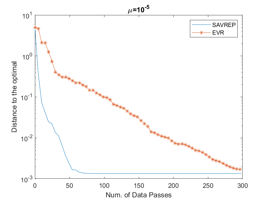
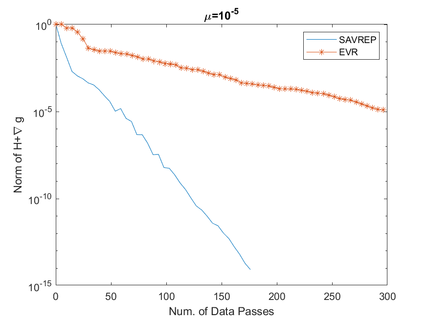
Figure 1: Convergence of SAVREP under perturbation $\mu=10^{-5}$

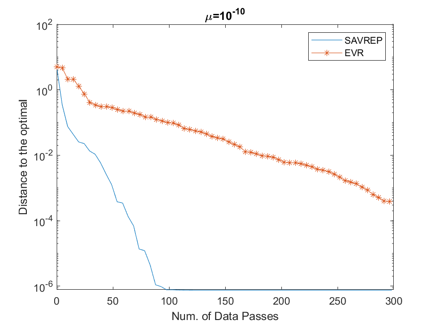
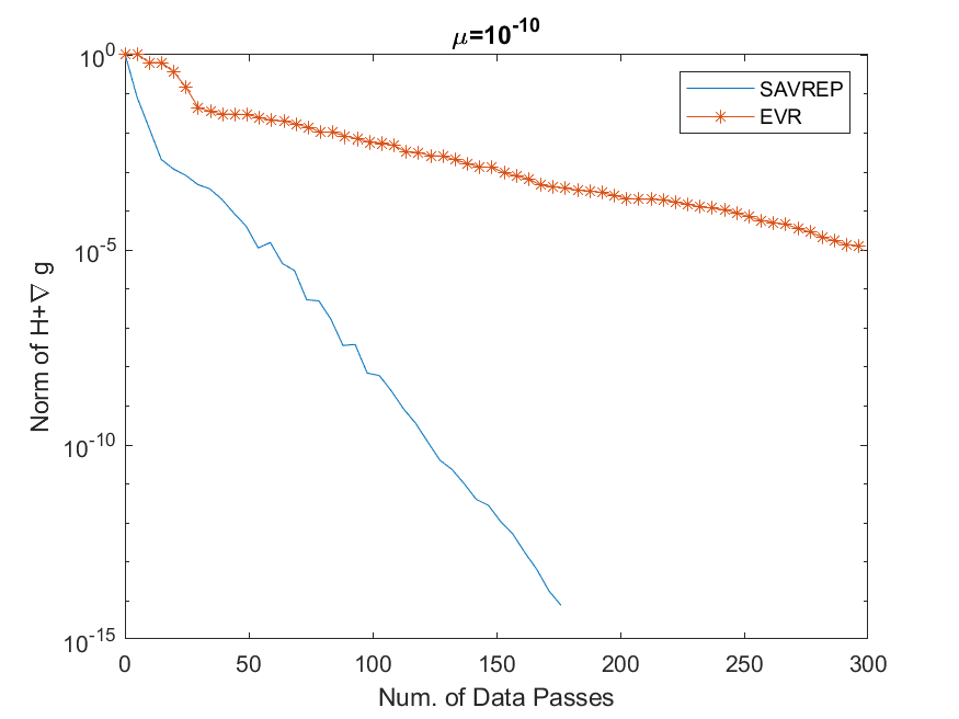
Figure 2: Convergence of SAVREP under perturbation $\mu=10^{-10}$

5.2 SAVREP-m

In this experiment, we test SAVREP-m on the same problem (71), using the VI formulation without perturbation (4.1). The parameter tuning is similar to the previous experiment, while the loss function is defined as the logistic loss function, i.e. $\phi(t)=\log(1+\exp(-t))$, with $\lambda=5$ and $r_{1}=0.4$. The convergence in terms of distance to optimal solution and norm of $H(x)+\nabla g(x)$ are shown in Figure 3. In addition, the constraint violation and objective function gap are shown in Figure 4. These results demonstrate the sublinear convergence rate of SAVREP-m, which is consistent with the theoretical guarantee derived in Section 3.1. On the other hand, EVR in this experiment shows a linear convergence rate similar to that in the previous experiment with perturbation. Note that in the second experiment the problem may still be (locally) strongly monotone after reformulation even without perturbation. While EVR does not require the strongly monotone modulus in its algorithm and reflects linear convergence automatically, we note that SAVREP-m explicitly assumes the problem to be merely monotone by using diminishing step sizes, as shown in Corollary 3.5. The specific design is necessary for SAVREP-m to guarantee a faster sublinear rate given the composite VI structure (7), at the cost of not being able to converge linearly when the problem is actually strongly monotone. We remark that the purpose of this experiment is to demonstrate the convergence behavior of SAVREP-m, and in practice it makes sense to apply SAVREP instead with estimated strong monotonicity modulus.

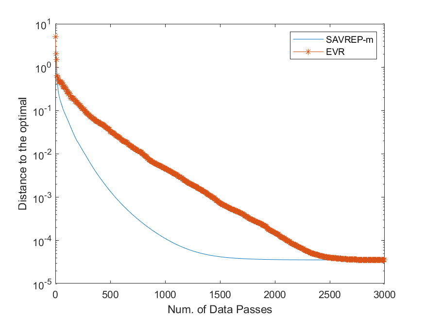
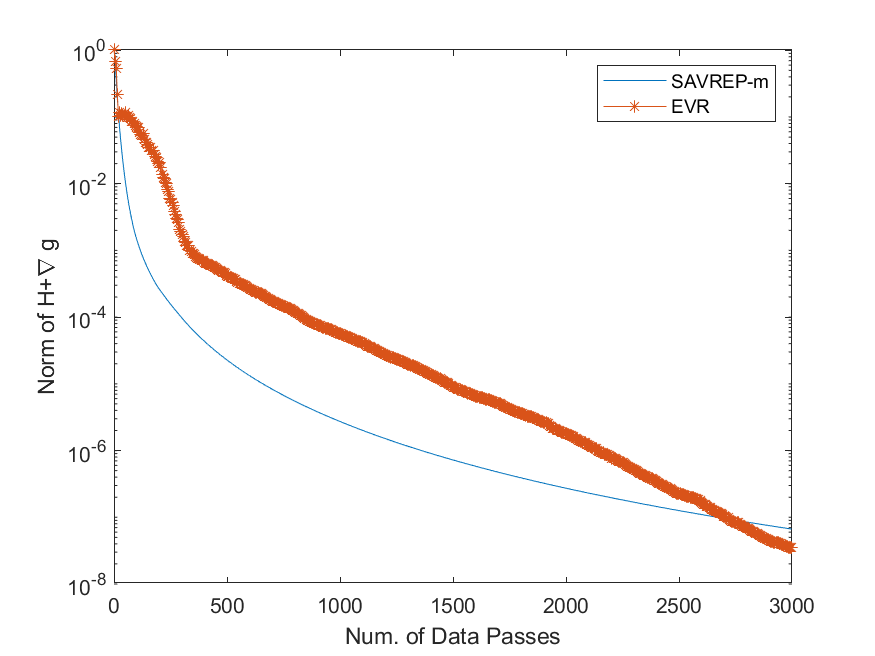
Figure 3: Convergence of SAVREP-m: distance to optimal solution (left) and norm of $H+\nabla g$ (right)

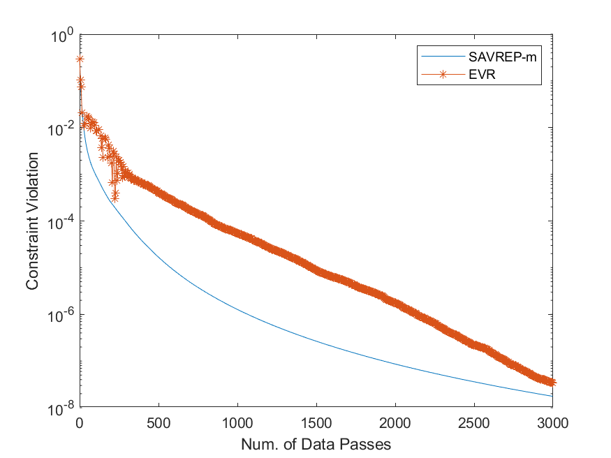
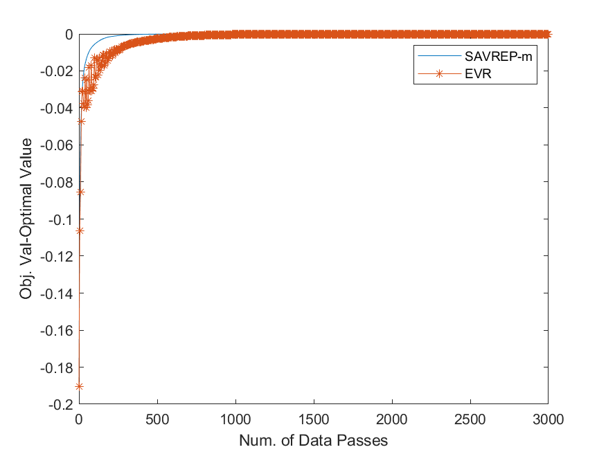
Figure 4: Convergence of SAVREP-m: constraint violation (left) and objective function gap (right)

6 Conclusions

In this paper, we propose two stochastic variance reduced schemes, SAVREP and SAVREP-m, for solving an extended class of finite-sum VI with strongly monotone operator and monotone operator respectively. The operator consists of the sum of a general VI mapping and a gradient mapping, both with finite-sum structure. By exploiting this special structure and applying variance reduction techniques developed in the literature, we show that both schemes admit improved gradient complexities, compared to existing variance reduction algorithms proposed for general finite-sum VI. In addition, we consider a more general stochastic setup in both proposed schemes, where the stochastic oracles of noisy mappings are adopted in the updates, and derive the corresponding stochastic bounds in the results of our complexity analysis. We show that an application of finite-sum optimization with finite-sum inequality constraints can be reformulated into the finite-sum VI of the special structure discussed in this paper, where the proposed schemes can be readily applied to. Finally, we note that while the established gradient complexity results match the optimal complexities in terms of problem constants in optimization (i.e. the constants related to the gradient mapping), the gap between the current lower bound established for finite-sum VI remains unfilled. It is still an open question whether the upper bound or the lower bound can be improved to match the other, and we leave it to future works.

Appendix A Proofs for Technical Results

A.1 Proof of Lemma 2.1

The optimality condition at $x^{k+0.5}$ yields

$$\langle\gamma\left({H^{\prime}}(w^{k})+\tilde{\nabla}{g^{\prime}}(y^{k})\right)+x^{k+0.5}-\bar{x}^{k},x-x^{k+0.5}\rangle\geq 0,\quad\forall x\in\mathcal{Z},$$ (76)

and the optimality condition at $x^{k+1}$ yields

$$\langle\gamma\left(\hat{H^{\prime}}(x^{k+0.5})+\tilde{\nabla}{g^{\prime}}(y^{k})\right)+x^{k+1}-\bar{x}^{k},x-x^{k+1}\rangle\geq 0,\quad\forall x\in\mathcal{Z}.$$ (77)

From (77), use the expression of $\bar{x}^{k}$:

$$\frac{1}{2}\left(\|x^{k+1}-x\|^{2}+(1-p_{1})\|x^{k+1}-x^{k}\|^{2}-(1-p_{1})\|x^{k}-x\|^{2}+p_{1}\|x^{k+1}-w^{k}\|^{2}-p_{1}\|w^{k}-x\|^{2}\right)$$

$$= (1-p_{1})\langle x^{k+1}-x^{k},x^{k+1}-x\rangle+p_{1}\langle x^{k+1}-w^{k},x^{k+1}-x\rangle\leq\gamma\langle\hat{{H^{\prime}}}(x^{k+0.5})+\tilde{\nabla}{g^{\prime}}(y^{k}),x-x^{k+1}\rangle,$$

where

$$\gamma\langle\hat{{H^{\prime}}}(x^{k+0.5})+\tilde{\nabla}{g^{\prime}}(y^{k}),x-x^{k+1}\rangle$$ (79)

$$= \gamma\langle\hat{{H^{\prime}}}(x^{k+0.5})+\tilde{\nabla}{g^{\prime}}(y^{k}),x-x^{k+0.5}\rangle+\gamma\langle\hat{{H^{\prime}}}(x^{k+0.5})+\tilde{\nabla}{g^{\prime}}(y^{k}),x^{k+0.5}-x^{k+1}\rangle$$

$$= \gamma\langle H(x^{k+0.5})+\tilde{\nabla}{g^{\prime}}(y^{k}),x-x^{k+0.5}\rangle+\gamma\langle\hat{{H^{\prime}}}(x^{k+0.5})-H(x^{k+0.5}),x-x^{k+0.5}\rangle$$

$$+\gamma\langle{H^{\prime}}(w^{k})+\tilde{\nabla}{g^{\prime}}(y^{k}),x^{k+0.5}-x^{k+1}\rangle+\gamma\langle\hat{{H^{\prime}}}(x^{k+0.5})-{H^{\prime}}(w^{k}),x^{k+0.5}-x^{k+1}\rangle.$$

The third term in the above inequality can be bounded by using (76) with $x=x^{k+1}$:

$$\gamma\langle{H^{\prime}}(w^{k})+\tilde{\nabla}{g^{\prime}}(y^{k}),x^{k+0.5}-x^{k+1}\rangle\leq\langle x^{k+0.5}-\bar{x}^{k},x^{k+1}-x^{k+0.5}\rangle$$

$$= (1-p_{1})\langle x^{k+0.5}-x^{k},x^{k+1}-x^{k+0.5}\rangle+p_{1}\langle x^{k+0.5}-w^{k},x^{k+1}-x^{k+0.5}\rangle$$

$$= \frac{1}{2}\left(-\|x^{k+1}-x^{k+0.5}\|^{2}+(1-p_{1})\|x^{k+1}-x^{k}\|^{2}-(1-p_{1})\|x^{k+0.5}-x^{k}\|^{2}\right.$$

$$\left.+p_{1}\|x^{k+1}-w^{k}\|^{2}-p_{1}\|x^{k+0.5}-w^{k}\|^{2}\right),$$

while the fourth term can be bounded by:

$$\gamma\langle\hat{{H^{\prime}}}(x^{k+0.5})-{H^{\prime}}(w^{k}),x^{k+0.5}-x^{k+1}\rangle=\gamma\langle{H}_{\xi_{k}}^{\prime}(x^{k+0.5})-{H}_{\xi_{k}}^{\prime}(w^{k}),x^{k+0.5}-x^{k+1}\rangle$$

$$\leq \frac{\gamma^{2}}{2}\|{H}_{\xi_{k}}^{\prime}(x^{k+0.5})-{H}_{\xi_{k}}^{\prime}(w^{k})\|^{2}+\frac{1}{2}\|x^{k+0.5}-x^{k+1}\|^{2}.$$

Combine the above two inequalities with (79) and use $\mathbb{E}_{k_{1}}[\cdot]:=\mathbb{E}_{\xi_{k}}[\cdot|x^{k},w^{k}]$:

$$\mathbb{E}_{k_{1}}\left[\gamma\langle\hat{{H^{\prime}}}(x^{k+0.5})+\tilde{\nabla}{g^{\prime}}(y^{k}),x-x^{k+1}\rangle\right]$$ (80)

$$\leq \mathbb{E}_{k_{1}}\left[\gamma\langle H(x^{k+0.5})+\tilde{\nabla}{g^{\prime}}(y^{k}),x-x^{k+0.5}\rangle\right]+\mathbb{E}_{k_{1}}\left[\gamma\langle\hat{H^{\prime}}(x^{k+0.5})-H(x^{k+0.5}),x-x^{k+0.5}\rangle\right]$$

$$+\frac{1}{2}\mathbb{E}_{k_{1}}\left[\gamma^{2}\|{H}_{\xi_{k}}^{\prime}(x^{k+0.5})-{H}_{\xi_{k}}^{\prime}(w^{k})\|^{2}+(1-p_{1})\|x^{k+1}-x^{k}\|^{2}\right.$$

$$\left.-(1-p_{1})\|x^{k+0.5}-x^{k}\|^{2}+p_{1}\|x^{k+1}-w^{k}\|^{2}-p_{1}\|x^{k+0.5}-w^{k}\|^{2}\right].$$

Let us bound the term $\mathbb{E}_{k_{1}}\left[\gamma\langle\hat{H}^{\prime}(x^{k+0.5})-H(x^{k+0.5}),x-x^{k+0.5}\rangle\right]$. Note that with $\mathbb{E}_{k_{1}}[\cdot]$, $x^{k+0.5}$ is deterministic and $\mathbb{E}_{k_{1}}\left[\hat{H}^{\prime}(x^{k+0.5})\right]=H^{\prime}(x^{k+0.5})$. Therefore,

$$\mathbb{E}_{k_{1}}\left[\gamma\langle\hat{H}^{\prime}(x^{k+0.5})-H(x^{k+0.5}),x-x^{k+0.5}\rangle\right]=\gamma\langle H^{\prime}(x^{k+0.5})-H(x^{k+0.5}),x-x^{k+0.5}\rangle$$ (81)

$$\leq \frac{\gamma}{2\mu_{h}}\left\|H^{\prime}(x^{k+0.5})-H(x^{k+0.5})\right\|^{2}+\frac{\gamma\mu_{h}}{2}\|x-x^{k+0.5}\|^{2}.$$

Continue with (80):

$$\mathbb{E}_{k_{1}}\left[\gamma\langle\hat{{H^{\prime}}}(x^{k+0.5})+\tilde{\nabla}{g^{\prime}}(y^{k}),x-x^{k+1}\rangle\right]$$

$$\leq \mathbb{E}_{k_{1}}\left[\gamma\langle H(x^{k+0.5})+\tilde{\nabla}{g^{\prime}}(y^{k}),x-x^{k+0.5}\rangle\right]+\frac{1}{2}\mathbb{E}_{k_{1}}\left[\gamma^{2}\|{H}_{\xi_{k}}^{\prime}(x^{k+0.5})-{H}_{\xi_{k}}^{\prime}(w^{k})\|^{2}\right]$$

$$+\frac{1}{2}\mathbb{E}_{k_{1}}\left[(1-p_{1})\|x^{k+1}-x^{k}\|^{2}-\left({1}-p_{1}\right)\|x^{k+0.5}-x^{k}\|^{2}+p_{1}\|x^{k+1}-w^{k}\|^{2}-p_{1}\|x^{k+0.5}-w^{k}\|^{2}\right]$$

$${+\frac{\gamma\bar{\varepsilon}_{x^{k+0.5}}^{2}}{2\mu_{h}}+\frac{1}{2}\mathbb{E}_{k_{1}}\left[\gamma\mu_{h}\|x^{k+0.5}-x\|^{2}\right]}.$$

Combine with (LABEL:VI-bd-0):

$$\frac{1}{2}\mathbb{E}_{k_{1}}\left[\|x^{k+1}-x\|^{2}-(1-p_{1})\|x^{k}-x\|^{2}-p_{1}\|w^{k}-x\|^{2}+\left(1-p_{1}\right)\|x^{k+0.5}-x^{k}\|^{2}\right]$$

$$+\mathbb{E}_{k_{1}}\left[\gamma\langle H(x^{k+0.5})+\tilde{\nabla}{g^{\prime}}(y^{k}),x^{k+0.5}-x\rangle\right]$$

$$\leq \frac{1}{2}\mathbb{E}_{k_{1}}\left[\gamma^{2}\|{H}_{\xi_{k}}^{\prime}(x^{k+0.5})-{H}_{\xi_{k}}^{\prime}(w^{k})\|^{2}-p_{1}\|x^{k+0.5}-w^{k}\|^{2}\right]{+\frac{\gamma\bar{\varepsilon}_{x^{k+0.5}}^{2}}{2\mu_{h}}+\frac{1}{2}\mathbb{E}_{k_{1}}\left[\gamma\mu_{h}\|x^{k+0.5}-x\|^{2}\right]}$$

$$\leq \frac{1}{2}({2}\gamma^{2}L_{h}^{2}-p_{1})\|x^{k+0.5}-w^{k}\|^{2}{+\frac{\gamma\bar{\varepsilon}_{x^{k+0.5}}^{2}}{2\mu_{h}}+\frac{1}{2}\mathbb{E}_{k_{1}}\left[\gamma\mu_{h}\|x^{k+0.5}-x\|^{2}\right]+\gamma^{2}\mathbb{E}_{k_{1}}\left[(\varepsilon_{x^{k+0.5}}+\varepsilon_{w^{k}})^{2}\right]}.$$

The last inequality is due to the following relation:

$$\mathbb{E}_{k_{1}}\left[\|H_{\xi_{k}}^{\prime}(x^{k+0.5})-H_{\xi_{k}}^{\prime}(w^{k})\|^{2}\right]$$ (82)

$$\leq \mathbb{E}_{k_{1}}\left[2\|H_{\xi_{k}}(x^{k+0.5})-H_{\xi_{k}}(w^{k})\|^{2}\right]+\mathbb{E}_{k_{1}}\left[2\left(\|H_{\xi_{k}}^{\prime}(x^{k+0.5})-H_{\xi_{k}}(x^{k+0.5})\|+\|H_{\xi_{k}}^{\prime}(w^{k})-H_{\xi_{k}}(w^{k})\|\right)^{2}\right]$$

$$\leq 2L_{h}^{2}\|x^{k+0.5}-w^{k}\|^{2}+2\mathbb{E}_{k_{1}}\left[\left(\varepsilon_{x^{k+0.5}}+\varepsilon_{w^{k}}\right)^{2}\right].$$

Rearrange the terms with the strong monotonicity of $H(\cdot)$:

$$\mathbb{E}_{k_{1}}\left[\gamma\langle H(x)+\tilde{\nabla}{g^{\prime}}(y^{k}),x^{k+0.5}-x\rangle+\gamma\mu_{h}\|x^{k+0.5}-x\|^{2}+\frac{1}{2}(p_{1}-{2}\gamma^{2}L^{2}_{h})\|x^{k+0.5}-w^{k}\|^{2}\right]$$

$$\leq \mathbb{E}_{k_{1}}\left[\gamma\langle H(x^{k+0.5})+\tilde{\nabla}{g^{\prime}}(y^{k}),x^{k+0.5}-x\rangle+\frac{1}{2}(p_{1}-{2}\gamma^{2}L^{2}_{h})\|x^{k+0.5}-w^{k}\|^{2}\right]$$

$$\leq \frac{1}{2}\mathbb{E}_{k_{1}}\left[-\|x^{k+1}-x\|^{2}+(1-p_{1})\|x^{k}-x\|^{2}+p_{1}\|w^{k}-x\|^{2}-\left(1-p_{1}\right)\|x^{k+0.5}-x^{k}\|^{2}\right]$$

$${+\frac{\gamma\bar{\varepsilon}_{x^{k+0.5}}^{2}}{2\mu_{h}}+\frac{1}{2}\mathbb{E}_{k_{1}}\left[\gamma\mu_{h}\|x^{k+0.5}-x\|^{2}\right]+\gamma^{2}\mathbb{E}_{k_{1}}\left[(\varepsilon_{x^{k+0.5}}+\varepsilon_{w^{k}})^{2}\right]},$$

which gives us

$$\mathbb{E}_{k_{1}}\left[\gamma\langle H(x)+\tilde{\nabla}{g^{\prime}}(y^{k}),x^{k+0.5}-x\rangle\right]$$ (83)

$$\leq \frac{1}{2}\mathbb{E}_{k_{1}}\left[(1-p_{1})\|x^{k}-x\|^{2}+p_{1}\|w^{k}-x\|^{2}-\|x^{k+1}-x\|^{2}\right]$$

$$-\frac{1}{2}\mathbb{E}_{k_{1}}\left[(p_{1}-{2}\gamma^{2}L_{h}^{2})\|x^{k+0.5}-w^{k}\|^{2}\right]-{\frac{1}{2}}\mathbb{E}_{k_{1}}\left[\gamma{\mu_{h}}\|x^{k+0.5}-x\|^{2}\right]-\frac{1}{2}\left(1-p_{1}\right)\|x^{k+0.5}-x^{k}\|^{2}$$

$${+\frac{\gamma\bar{\varepsilon}_{x^{k+0.5}}^{2}}{2\mu_{h}}+\gamma^{2}\mathbb{E}_{k_{1}}\left[(\varepsilon_{x^{k+0.5}}+\varepsilon_{w^{k}})^{2}\right]}$$

$$\leq \frac{1}{2}\mathbb{E}_{k_{1}}\left[(1-p_{1})\|x^{k}-x\|^{2}+p_{1}\|w^{k}-x\|^{2}-\|x^{k+1}-x\|^{2}\right]$$

$$-\frac{1}{2}\mathbb{E}_{k_{1}}\left[(p_{1}-{2}\gamma^{2}L_{h}^{2})\|x^{k+0.5}-w^{k}\|^{2}\right]-\mathbb{E}_{k_{1}}\left[\frac{1}{{4}}\gamma{\mu_{h}}\|x^{k}-x\|^{2}-{\frac{1}{2}}\gamma\mu_{h}\|x^{k+0.5}-x^{k}\|^{2}\right]$$

$$-\frac{1}{2}\left(1-p_{1}\right)\mathbb{E}_{k_{1}}\left[\|x^{k+0.5}-x^{k}\|^{2}\right]{+\frac{\gamma\bar{\varepsilon}_{x^{k+0.5}}^{2}}{2\mu_{h}}+\gamma^{2}\mathbb{E}_{k_{1}}\left[(\varepsilon_{x^{k+0.5}}+\varepsilon_{w^{k}})^{2}\right]}$$

$$\leq \frac{1}{2}\mathbb{E}_{k_{1}}\left[(1-p_{1}-{\frac{1}{2}}\gamma\mu_{h})\|x^{k}-x\|^{2}+p_{1}\|w^{k}-x\|^{2}-\|x^{k+1}-x\|^{2}\right]$$

$$-\frac{1}{2}\left(p_{1}-{2}\gamma^{2}L_{h}^{2}\right)\mathbb{E}_{k_{1}}\left[\|x^{k+0.5}-w^{k}\|^{2}\right]-\frac{1}{2}\left(1-p_{1}-\gamma\mu_{h}\right)\mathbb{E}_{k_{1}}\left[\|x^{k+0.5}-x^{k}\|^{2}\right]$$

$${+\frac{\gamma\bar{\varepsilon}_{x^{k+0.5}}^{2}}{2\mu_{h}}+\gamma^{2}\mathbb{E}_{k_{1}}\left[(\varepsilon_{x^{k+0.5}}+\varepsilon_{w^{k}})^{2}\right]},$$

completing the proof.

A.2 Proof of Lemma 2.2

Using the Lipchistz continuity of $g(\cdot)$:

$$g(v^{k+1}) \leq g(y^{k})+\langle\nabla g(y^{k}),v^{k+1}-y^{k}\rangle+\frac{L_{g}}{2}\|v^{k+1}-y^{k}\|^{2}$$ (84)

$$= g(y^{k})+\langle\nabla g(y^{k}),(1-\alpha-\beta)v^{k}+\alpha x^{k+0.5}+\beta\bar{w}^{k}-y^{k}\rangle+\frac{L_{g}\alpha^{2}}{2}\|x^{k+0.5}-x^{k}\|^{2}$$

$$= (1-\alpha-\beta)\left(g(y^{k})+\langle\nabla g(y^{k}),v^{k}-y^{k}\rangle\right)+\alpha\left(g(y^{k})+\langle\nabla g(y^{k}),x^{k+0.5}-y^{k}\rangle\right)$$

$$+\beta\left(g(y^{k})+\langle\nabla g(y^{k}),\bar{w}^{k}-y^{k}\rangle\right)+\frac{L_{g}\alpha^{2}}{2}\|x^{k+0.5}-x^{k}\|^{2}$$

$$\leq (1-\alpha-\beta)g(v^{k})+\alpha\left(g(x)+\langle\nabla g(y^{k}),x^{k+0.5}-x\rangle\right)$$

$$+\beta\left(g(y^{k})+\langle\nabla g(y^{k}),\bar{w}^{k}-y^{k}\rangle\right)+\frac{L_{g}\alpha^{2}}{2}\|x^{k+0.5}-x^{k}\|^{2}$$

$$= (1-\alpha-\beta)g(v^{k})+\beta\left(g(y^{k})+\langle\nabla g(y^{k}),\bar{w}^{k}-y^{k}\rangle\right)+\frac{L_{g}\alpha^{2}}{2}\|x^{k+0.5}-x^{k}\|^{2}$$

$$+\alpha\left(g(x)+\langle\tilde{\nabla}{g^{\prime}}(y^{k}),x^{k+0.5}-x\rangle+\langle\nabla g(y^{k})-\tilde{\nabla}g(y^{k}),x^{k+0.5}-x\rangle\right)$$

$$+\alpha\langle\tilde{\nabla}g(y^{k})-\tilde{\nabla}{g^{\prime}}(y^{k}),x^{k+0.5}-x\rangle.$$

Let us first bound the last term $\alpha\langle\tilde{\nabla}g(y^{k})-\tilde{\nabla}{g^{\prime}}(y^{k}),x^{k+0.5}-x\rangle$ in the above inequality (84). By taking the expectation $\mathbb{E}_{k_{2}}[\cdot]$:

$$\alpha\mathbb{E}_{k_{2}}\left[\langle\tilde{\nabla}g(y^{k})-\tilde{\nabla}{g^{\prime}}(y^{k}),x^{k+0.5}-x\rangle\right]$$

$$\leq \mathbb{E}_{k_{2}}\left[\frac{4\alpha}{\mu_{h}}\left\|\tilde{\nabla}g(y^{k})-\tilde{\nabla}{g^{\prime}}(y^{k})\right\|^{2}\right]+\mathbb{E}_{k_{2}}\left[\frac{\alpha\mu_{h}}{16}\|x^{k+0.5}-x\|^{2}\right]$$

$$\leq \mathbb{E}_{k_{2}}\left[\frac{4\alpha}{\mu_{h}}\left\|\tilde{\nabla}g(y^{k})-\tilde{\nabla}{g^{\prime}}(y^{k})\right\|^{2}\right]+\mathbb{E}_{k_{2}}\left[\frac{\alpha\mu_{h}}{8}\|x^{k+0.5}-x^{k}\|^{2}\right]+\mathbb{E}_{k_{2}}\left[\frac{\alpha\mu_{h}}{8}\|x^{k}-x\|^{2}\right].$$

Note that

$$\mathbb{E}_{k_{2}}\left[\left\|\tilde{\nabla}g(y^{k})-\tilde{\nabla}{g^{\prime}}(y^{k})\right\|^{2}\right]$$

$$\leq \mathbb{E}_{k_{2}}\left[\left(\|\nabla g(\bar{w}^{k})-\nabla g^{\prime}(\bar{w}^{k})\|+\|\nabla g_{\zeta_{k}}(\bar{w}^{k})-\nabla g_{\zeta_{k}}^{\prime}(\bar{w}^{k})\|+\|\nabla g_{\zeta_{k}}(y^{k})-\nabla g_{\zeta_{k}}^{\prime}(y^{k})\|\right)^{2}\right]$$

$$\leq 2\bar{\rho}_{\bar{w}^{k}}^{2}+2\mathbb{E}_{k_{2}}\left[(\rho_{\bar{w}^{k}}+\rho_{y^{k}})^{2}\right].$$

Also note that:

$$\mathbb{E}_{k_{2}}\left[\langle\nabla g(y^{k})-\tilde{\nabla}g(y^{k}),x^{k+0.5}-x\rangle\right]=\mathbb{E}_{k_{2}}\left[\langle\nabla g(y^{k})-\tilde{\nabla}g(y^{k}),x^{k+0.5}-x^{k}\rangle\right]$$ (86)

$$\leq \mathbb{E}_{k_{2}}\left[\frac{\beta}{2\alpha L_{g}}\|\nabla g(y^{k})-\tilde{\nabla}g(y^{k})\|^{2}\right]+\mathbb{E}_{k_{2}}\left[\frac{\alpha L_{g}}{2\beta}\|x^{k+0.5}-x^{k}\|^{2}\right]$$

$$\leq \frac{\beta}{\alpha}\left(g(\bar{w}^{k})-g(y^{k})-\langle\nabla g(y^{k}),\bar{w}^{k}-y^{k}\rangle\right)+\mathbb{E}_{k_{2}}\left[\frac{\alpha L_{g}}{2\beta}\|x^{k+0.5}-x^{k}\|^{2}\right].$$

In the second inequality, we use the following relation:

$$\mathbb{E}_{k_{2}}\left[\|\nabla g(y^{k})-\tilde{\nabla}g(y^{k})\|^{2}\right]=\mathbb{E}_{k_{2}}\left[\|\nabla g_{\zeta_{k}}(\bar{w}^{k})-\nabla g_{\zeta_{k}}(y^{k})-\left(\nabla g(\bar{w}^{k})-\nabla g(y^{k})\right)\|^{2}\right]$$ (87)

$$\leq \mathbb{E}_{k_{2}}\left[\|\nabla g_{\zeta_{k}}(\bar{w}^{k})-\nabla g_{\zeta_{k}}(y^{k})\|^{2}\right]=\sum\limits_{i=1}^{m_{2}}\frac{1}{\pi_{i}}\|\nabla g_{i}(\bar{w}^{k})-\nabla g_{i}(y^{k})\|^{2}$$

$$\leq \sum\limits_{i=1}^{m_{2}}\frac{2L_{g(i)}}{\pi_{i}}\left(g_{i}(\bar{w}^{k})-g_{i}(y^{k})-\langle\nabla g_{i}(y^{k}),\bar{w}^{k}-y^{k}\rangle\right)=2L_{g}\sum\limits_{i=1}^{m_{2}}\left(g_{i}(\bar{w}^{k})-g_{i}(y^{k})-\langle\nabla g_{i}(y^{k}),\bar{w}^{k}-y^{k}\rangle\right)$$

$$= 2L_{g}\left(g(\bar{w}^{k})-g(y^{k})-\langle\nabla g(y^{k}),\bar{w}^{k}-y^{k}\rangle\right),$$

where the first inequality is from $\mathbb{E}\|\zeta-\mathbb{E}\zeta\|^{2}=\mathbb{E}\|\zeta\|^{2}-\|\mathbb{E}\zeta\|^{2}\leq\mathbb{E}\|\zeta\|^{2}$ and the second inequality is from Theorem 2.1.5 in [23]

Combine (84), (LABEL:sto-bias-bd-opt) and (86):

$$\mathbb{E}_{k_{2}}\left[g(v^{k+1})\right] \leq \mathbb{E}_{k_{2}}\left[(1-\alpha-\beta)g(v^{k})+\alpha g(x)+\beta g(\bar{w}^{k})\right]$$

$$+\mathbb{E}_{k_{2}}\left[\alpha\langle\tilde{\nabla}g^{\prime}(y^{k}),x^{k+0.5}-x\rangle\right]+{\left(\frac{\alpha^{2}L_{g}}{2}+\frac{\alpha^{2}L_{g}}{2\beta}+\frac{\alpha\mu_{h}}{8}\right)}\mathbb{E}_{k_{2}}\left[\|x^{k+0.5}-x^{k}\|^{2}\right]$$

$$+{\frac{\alpha\mu_{h}}{8}\mathbb{E}_{k_{2}}\left[\|x^{k}-x\|^{2}\right]+\frac{8\alpha}{\mu_{h}}\mathbb{E}_{k_{2}}[\bar{\rho}_{\bar{w}^{k}}^{2}]+\frac{8\alpha}{\mu_{h}}\mathbb{E}_{k_{2}}\left[(\rho_{\bar{w}^{k}}+\rho_{y^{k}})^{2}\right]},$$

implying

$$\mathbb{E}_{k_{2}}\left[g(v^{k+1})-g(x)\right] \leq \mathbb{E}_{k_{2}}\left[(1-\alpha-\beta)\left(g(v^{k})-g(x)\right)+\beta\left(g(\bar{w}^{k})-g(x)\right)\right]$$

$$+\mathbb{E}_{k_{2}}\left[\alpha\langle\tilde{\nabla}g^{\prime}(y^{k}),x^{k+0.5}-x\rangle\right]+{\left(\frac{\alpha^{2}L_{g}}{2}+\frac{\alpha^{2}L_{g}}{2\beta}+\frac{\alpha\mu_{h}}{8}\right)}\mathbb{E}_{k_{2}}\left[\|x^{k+0.5}-x^{k}\|^{2}\right]$$

$$+{\frac{\alpha\mu_{h}}{8}\mathbb{E}_{k_{2}}\left[\|x^{k}-x\|^{2}\right]+\frac{8\alpha}{\mu_{h}}\mathbb{E}_{k_{2}}[\bar{\rho}_{\bar{w}^{k}}^{2}]+\frac{8\alpha}{\mu_{h}}\mathbb{E}_{k_{2}}\left[(\rho_{\bar{w}^{k}}+\rho_{y^{k}})^{2}\right]},$$

completing the proof.

A.3 Proof of Theorem 2.3

In view of Lemma 2.1 and Lemma 2.2, we can establish the following inequality

$$\mathbb{E}_{k_{2}}\left[Q(v^{k+1};x)\right]$$

$$= \mathbb{E}_{k_{2}}\left[\langle H(x),v^{k+1}-x\rangle+g(v^{k+1})-g(x)\right]$$

$$= \mathbb{E}_{k_{2}}\left[(1-\alpha-\beta)\langle H(x),v^{k}-x\rangle+\alpha\langle H(x),x^{k+0.5}-x\rangle+\beta\langle H(x),\bar{w}^{k}-x\rangle\right]+\mathbb{E}_{k_{2}}\left[g(v^{k+1})-g(x)\right]$$

$$\leq \mathbb{E}_{k_{2}}\left[(1-\alpha-\beta)\langle H(x),v^{k}-x\rangle+\alpha\langle H(x),x^{k+0.5}-x\rangle+\beta\langle H(x),\bar{w}^{k}-x\rangle\right]$$

$$+\mathbb{E}_{k_{2}}\left[(1-\alpha-\beta)\left(g(v^{k})-g(x)\right)+\beta\left(g(\bar{w}^{k})-g(x)\right)\right]$$

$$+\mathbb{E}_{k_{2}}\left[\alpha\langle\tilde{\nabla}g^{\prime}(y^{k}),x^{k+0.5}-x\rangle\right]+{\left(\frac{\alpha^{2}L_{g}}{2}+\frac{\alpha^{2}L_{g}}{2\beta}+\frac{\alpha\mu_{h}}{8}\right)}\mathbb{E}_{k_{2}}\left[\|x^{k+0.5}-x^{k}\|^{2}\right]$$

$${+\frac{\alpha\mu_{h}}{8}\mathbb{E}_{k_{2}}\left[\|x^{k}-x\|^{2}\right]+\frac{8\alpha}{\mu_{h}}\mathbb{E}_{k_{2}}[\bar{\rho}_{\bar{w}^{k}}^{2}]+\frac{8\alpha}{\mu_{h}}\mathbb{E}_{k_{2}}\left[(\rho_{\bar{w}^{k}}+\rho_{y^{k}})^{2}\right]}$$

$$= (1-\alpha-\beta)\mathbb{E}_{k_{2}}\left[\langle H(x),v^{k}-x\rangle+g(v^{k})-g(x)\right]+\beta\mathbb{E}_{k_{2}}\left[\langle H(x),\bar{w}^{k}-x\rangle+g(\bar{w}^{k})-g(x)\right]$$

$$+\alpha\mathbb{E}_{k_{2}}\left[\langle H(x)+\tilde{\nabla}g^{\prime}(y^{k}),x^{k+0.5}-x\rangle+{\left(\frac{\alpha L_{g}}{2}+\frac{\alpha L_{g}}{2\beta}+\frac{\mu_{h}}{8}\right)}\|x^{k+0.5}-\bar{x}^{k}\|^{2}\right]$$

$$+{\frac{\alpha\mu_{h}}{8}\mathbb{E}_{k_{2}}\left[\|x^{k}-x\|^{2}\right]+\frac{8\alpha}{\mu_{h}}\mathbb{E}_{k_{2}}[\bar{\rho}_{\bar{w}^{k}}^{2}]+\frac{8\alpha}{\mu_{h}}\mathbb{E}_{k_{2}}\left[(\rho_{\bar{w}^{k}}+\rho_{y^{k}})^{2}\right]}$$

$$\leq (1-\alpha-\beta)\mathbb{E}_{k_{2}}\left[Q(v^{k};x)\right]+\beta\mathbb{E}_{k_{2}}\left[Q(\bar{w}^{k};x)\right]$$

$$+\frac{\alpha}{2\gamma}\mathbb{E}_{k_{2}}\left[\left(1-p_{1}-{\frac{1}{2}}\gamma\mu_{h}+{\frac{\gamma\mu_{h}}{4}}\right)\|x^{k}-x\|^{2}+p_{1}\|w^{k}-x\|^{2}-\|x^{k+1}-x\|^{2}\right]$$

$$-\frac{\alpha}{2\gamma}\left(p_{1}-{2}\gamma^{2}L_{h}^{2}\right)\mathbb{E}_{k_{2}}\left[\|x^{k+0.5}-w^{k}\|^{2}\right]-\frac{\alpha}{2\gamma}\left(1-p_{1}-\gamma\mu_{h}-\alpha\gamma L_{g}-\frac{\alpha\gamma L_{g}}{\beta}-{\frac{\gamma\mu_{h}}{4}}\right)\mathbb{E}_{k_{2}}\left[\|x^{k+0.5}-x^{k}\|^{2}\right]$$

$${+\frac{\alpha\mathbb{E}_{k_{2}}\left[\bar{\varepsilon}_{x^{k+0.5}}^{2}\right]}{2\mu_{h}}+\alpha\gamma\mathbb{E}_{k_{2}}\left[(\varepsilon_{x^{k+0.5}}+\varepsilon_{w^{k}})^{2}\right]}+{\frac{8\alpha}{\mu_{h}}\mathbb{E}_{k_{2}}[\bar{\rho}_{\bar{w}^{k}}^{2}]+\frac{8\alpha}{\mu_{h}}\mathbb{E}_{k_{2}}\left[(\rho_{\bar{w}^{k}}+\rho_{y^{k}})^{2}\right]},$$

where the last inequality is due to Lemma 2.1.

Our goal now is to construct a proper potential function while keeping the coefficients of $\|x^{k+0.5}-w^{k}\|^{2}$ and $\|x^{k+0.5}-x^{k}\|^{2}$ non-positive. To this end, let us introduce the following bound while noting the expectation $\mathbb{E}_{k_{1}+}[\cdot]:=\mathbb{E}[\cdot|w^{k},x^{k+1}]$:

$$\mathbb{E}_{k_{2}}\left[\|w^{k+1}-x\|^{2}\right] = \mathbb{E}_{k_{2}}\left[\mathbb{E}_{k_{1}+}\left[\|w^{k+1}-x\|^{2}\right]\right]=p_{1}\mathbb{E}_{k_{2}}\left[\|x^{k+1}-x\|^{2}\right]+(1-p_{1})\mathbb{E}_{k_{2}}\left[\|w^{k}-x\|^{2}\right]$$

$$= \mathbb{E}_{k_{2}}\left[p_{1}\|x^{k+1}-x\|^{2}+(1-p_{1}-c)\|w^{k}-x\|^{2}+c\|w^{k}-x\|^{2}\right]$$

$$\leq \mathbb{E}_{k_{2}}\left[p_{1}\|x^{k+1}-x\|^{2}+(1-p_{1}-c)\|w^{k}-x\|^{2}\right]$$

$$+\mathbb{E}_{k_{2}}\left[2c\|x^{k}-x\|^{2}+4c\|x^{k}-x^{k+0.5}\|^{2}+4c\|x^{k+0.5}-w^{k}\|^{2}\right],$$

where $c>0$ is a parameter that needs to satisfy certain constraints to be determined later. Combine the above inequality with the previous inequality on $Q(v^{k+1};x)$, we have:

$$\mathbb{E}_{k_{2}}\left[Q(v^{k+1};x)\right]+\frac{\alpha}{2\gamma}\mathbb{E}_{k_{2}}\left[(1-p_{1})\|x^{k+1}-x\|^{2}+\|w^{k+1}-x\|^{2}\right]$$ (88)

$$\leq (1-\alpha-\beta)\mathbb{E}_{k_{2}}\left[Q(v^{k};x)\right]+\beta\mathbb{E}_{k_{2}}\left[Q(\bar{w}^{k};x)\right]$$

$$+\frac{\alpha}{2\gamma}\mathbb{E}_{k_{2}}\left[(1-p_{1}-{\frac{1}{4}}\gamma\mu_{h}+2c)\|x^{k}-x\|^{2}+(1-c)\|w^{k}-x\|^{2}\right]$$

$$-\frac{\alpha}{2\gamma}\left(p_{1}-{2}\gamma^{2}L_{h}^{2}-4c\right)\mathbb{E}_{k_{2}}\left[\|x^{k+0.5}-w^{k}\|^{2}\right]$$

$$-\frac{\alpha}{2\gamma}\left(1-p_{1}-{\frac{5}{4}}\gamma\mu_{h}-\alpha\gamma L_{g}-\frac{\alpha\gamma L_{g}}{\beta}-4c\right)\mathbb{E}_{k_{2}}\left[\|x^{k+0.5}-x^{k}\|^{2}\right]$$

$${+\frac{\alpha\mathbb{E}_{k_{2}}\left[\bar{\varepsilon}_{x^{k+0.5}}^{2}\right]}{2\mu_{h}}+\alpha\gamma\mathbb{E}_{k_{2}}\left[(\varepsilon_{x^{k+0.5}}+\varepsilon_{w^{k}})^{2}\right]}+{\frac{8\alpha}{\mu_{h}}\mathbb{E}_{k_{2}}[\bar{\rho}_{\bar{w}^{k}}^{2}]+\frac{8\alpha}{\mu_{h}}\mathbb{E}_{k_{2}}\left[(\rho_{\bar{w}^{k}}+\rho_{y^{k}})^{2}\right]}.$$

By imposing the following constraints on $c$:

$$\left\{\begin{array}[]{ll}1-{\frac{1}{4}}\gamma\mu_{h}+2c\leq 1,\\ 1-{\frac{1}{4}}\gamma\mu_{h}+2c\geq 1-c\end{array}\right.\Longleftrightarrow\frac{\gamma\mu_{h}}{12}\leq c\leq\frac{\gamma\mu_{h}}{{8}},$$ (91)

let us first take $c=\frac{\gamma\mu_{h}}{12}$ and impose another set of constraints on $\gamma$ and $\alpha$:

$$\left\{\begin{array}[]{ll}p_{1}-{2}\gamma^{2}L_{h}^{2}-\frac{\gamma\mu_{h}}{3}\geq 0,\\ 1-p_{1}-{\frac{19\gamma\mu_{h}}{12}}-\alpha\gamma L_{g}-\frac{\alpha\gamma L_{g}}{\beta}\geq 0,\end{array}\right.$$ (92)

then (88) can be reduced to:

$$\mathbb{E}_{k_{2}}\left[Q(v^{k+1};x)\right]+\frac{\alpha}{2\gamma}\mathbb{E}_{k_{2}}\left[(1-p_{1})\|x^{k+1}-x\|^{2}+\|w^{k+1}-x\|^{2}\right]$$

$$\leq (1-\alpha-\beta)\mathbb{E}_{k_{2}}\left[Q(v^{k};x)\right]+\beta\mathbb{E}_{k_{2}}\left[Q(\bar{w}^{k};x)\right]{+\frac{\alpha E_{k_{2}}\left[\bar{\varepsilon}_{x^{k+0.5}}^{2}\right]}{2\mu_{h}}+\alpha\gamma\mathbb{E}_{k_{2}}\left[(\varepsilon_{x^{k+0.5}}+\varepsilon_{w^{k}})^{2}\right]}$$

$$+\frac{\alpha}{2\gamma}\mathbb{E}_{k_{2}}\left[\left(1-p_{1}-\frac{\gamma\mu_{h}}{12}\right)\|x^{k}-x\|^{2}+\left(1-\frac{\gamma\mu_{h}}{12}\right)\|w^{k}-x\|^{2}\right]+{\frac{8\alpha}{\mu_{h}}\mathbb{E}_{k_{2}}[\bar{\rho}_{\bar{w}^{k}}^{2}]+\frac{8\alpha}{\mu_{h}}\mathbb{E}_{k_{2}}\left[(\rho_{\bar{w}^{k}}+\rho_{y^{k}})^{2}\right]}$$

$$\leq (1-\alpha-\beta)\mathbb{E}_{k_{2}}\left[Q(v^{k};x)\right]+\beta\mathbb{E}_{k_{2}}\left[Q(\bar{w}^{k};x)\right]{+\frac{\alpha\mathbb{E}_{k_{2}}\left[\bar{\varepsilon}_{x^{k+0.5}}^{2}\right]}{2\mu_{h}}+\alpha\gamma\mathbb{E}_{k_{2}}\left[(\varepsilon_{x^{k+0.5}}+\varepsilon_{w^{k}})^{2}\right]}$$

$$+\left(1-\frac{\gamma\mu_{h}}{12}\right)\frac{\alpha}{2\gamma}\mathbb{E}_{k_{2}}\left[\left(1-p_{1}\right)\|x^{k}-x\|^{2}+\|w^{k}-x\|^{2}\right]+{\frac{8\alpha}{\mu_{h}}\mathbb{E}_{k_{2}}[\bar{\rho}_{\bar{w}^{k}}^{2}]+\frac{8\alpha}{\mu_{h}}\mathbb{E}_{k_{2}}\left[(\rho_{\bar{w}^{k}}+\rho_{y^{k}})^{2}\right]}.$$

Now we only need to add the term $Q(\bar{w}^{k+1};x)$ to the LHS, by noting:

$$\phi\mathbb{E}_{k_{2}}\left[Q(\bar{w}^{k+1};x)\right] = \phi\mathbb{E}_{k_{2}}\left[\mathbb{E}_{k_{2}+}\left[Q(\bar{w}^{k+1};x)\right]\right]$$

$$= \phi p_{2}\mathbb{E}_{k_{2}}\left[Q(v^{k+1};x)\right]+\phi(1-p_{2})\mathbb{E}_{k_{2}}\left[Q(\bar{w}^{k};x)\right],$$

for any $\phi>0$.

Add the above identity to the previous inequality and take the total expectation, we have:

$$\mathbb{E}\left[(1-\phi p_{2})Q(v^{k+1};x)+\phi Q(\bar{w}^{k+1};x)\right]+\frac{\alpha}{2\gamma}\mathbb{E}\left[(1-p_{1})\|x^{k+1}-x\|^{2}+\|w^{k+1}-x\|^{2}\right]$$ (93)

$$\leq \mathbb{E}\left[(1-\alpha-\beta)Q(v^{k};x)+(\beta+\phi(1-p_{2}))Q(\bar{w}^{k};x)\right]+\left(1-\frac{\gamma\mu_{h}}{12}\right)\frac{\alpha}{2\gamma}\mathbb{E}\left[\left(1-p_{1}\right)\|x^{k}-x\|^{2}+\|w^{k}-x\|^{2}\right]$$

$$+\mathbb{E}\left[{\frac{\alpha\mathbb{E}_{k_{2}}\left[\bar{\varepsilon}_{x^{k+0.5}}^{2}\right]}{2\mu_{h}}+\alpha\gamma\mathbb{E}_{k_{2}}\left[(\varepsilon_{x^{k+0.5}}+\varepsilon_{w^{k}})^{2}\right]}+{\frac{8\alpha}{\mu_{h}}\mathbb{E}_{k_{2}}[\bar{\rho}_{\bar{w}^{k}}^{2}]+\frac{8\alpha}{\mu_{h}}\mathbb{E}_{k_{2}}\left[(\rho_{\bar{w}^{k}}+\rho_{y^{k}})^{2}\right]}\right],$$

where

$$\left\{\begin{array}[]{ll}\mathbb{E}\left[\mathbb{E}_{k_{2}}\left[\bar{\varepsilon}_{x^{k+0.5}}^{2}\right]\right]=\mathbb{E}\left[\mathbb{E}^{\prime}\left[\bar{\varepsilon}_{x^{k+0.5}}^{2}\right]\right]\leq 2m_{1}\sigma_{h}^{2}+2m_{1}^{2}\delta_{h}^{2}\\ \mathbb{E}\left[\mathbb{E}_{k_{2}}\left[(\varepsilon_{x^{k+0.5}}+\varepsilon_{w^{k}})^{2}\right]\right]=\mathbb{E}\left[\mathbb{E}^{\prime}\left[(\varepsilon_{x^{k+0.5}}+\varepsilon_{w^{k}})^{2}\right]\right]\leq 2\cdot\left(2L_{h}\cdot(\sigma_{h}^{2}+\delta_{h}^{2})\cdot\sum\limits_{i=1}^{m_{1}}\frac{1}{L_{h(i)}}\right)=2\tilde{\sigma}_{h}^{2}.\end{array}\right.$$ (96)

$$\left\{\begin{array}[]{ll}\mathbb{E}\left[\mathbb{E}_{k_{2}}[\bar{\rho}_{\bar{w}^{k}}^{2}]\right]=\mathbb{E}\left[\mathbb{E}^{\prime}[\bar{\rho}_{\bar{w}^{k}}^{2}]\right]\leq 2m_{2}\sigma_{g}^{2}+2m_{2}^{2}\delta_{g}^{2}\\ \mathbb{E}\left[\mathbb{E}_{k_{2}}\left[(\rho_{\bar{w}^{k}}+\rho_{y^{k}})^{2}\right]\right]=\mathbb{E}\left[\mathbb{E}^{\prime}\left[(\rho_{\bar{w}^{k}}+\rho_{y^{k}})^{2}\right]\right]\leq 2\cdot\left(2L_{g}\cdot(\sigma_{g}^{2}+\delta_{g}^{2})\cdot\sum\limits_{i=1}^{m_{2}}\frac{1}{L_{g(i)}}\right)=2\tilde{\sigma}_{g}^{2}.\end{array}\right.$$ (99)

By taking $x=x^{*}$ in (93) together with the expression of $\Delta_{h}$ and $\Delta_{g}$, we obtain (20), thus complete the proof.

A.4 Proof of Proposition 2.4

We first show that the parameters specified in Proposition 2.4 satisfy the constraint (92). Indeed, the constraints will be reduced to the following:

$$p_{1}-\frac{p_{1}}{8}-\frac{p_{1}}{12}\geq 0,\quad\frac{15}{16}-\frac{67p_{1}}{48}\geq 0,$$

where the second inequality holds because $p_{1}=\frac{1}{m_{1}}$ and we assume trivially that $m_{1}\geq 2$.

Next, inequality (20) in Theorem 2.3 implies that the reduction rate is given by:

$$C_{\scriptsize\mbox{red}1}:=\max\left\{\frac{1-\alpha-\beta}{1-\phi p_{2}},\frac{\beta+\phi(1-p_{2})}{\phi},1-\frac{\gamma\mu_{h}}{12}\right\}.$$

With the choice of $\phi$ and $p_{2}$, the following bounds hold:

$$\frac{1-\alpha-\beta}{1-\phi p_{2}}=\frac{1-2\alpha}{1-\alpha}\leq 1-\alpha,$$

and

$$\frac{\beta+\phi(1-p_{2})}{\phi}=1-\frac{1}{m_{2}}+\frac{1}{(1+\alpha)m_{2}}=1-\frac{\alpha}{(1+\alpha)m_{2}}\leq 1-\frac{\alpha}{2m_{2}}.$$

Therefore, the reduction rate is can be further expressed as

$$\max\left\{\frac{1-\alpha-\beta}{1-\phi p_{2}},\frac{\beta+\phi(1-p_{2})}{\phi},1-\frac{\gamma\mu_{h}}{12}\right\}\leq\max\left\{1-\alpha,1-\frac{\alpha}{2m_{2}},1-\frac{\gamma\mu_{h}}{12}\right\}$$

$$= \max\left\{1-\frac{\alpha}{2m_{2}},1-\frac{\gamma\mu_{h}}{12}\right\}$$

$$= {\max\left\{\max\left(1-\frac{\sqrt{\mu_{h}}}{24\sqrt{L_{g}m_{2}}},1-\frac{1}{24m_{2}}\right),\max\left(1-\frac{\mu_{h}}{48L_{h}\sqrt{m_{1}}},1-\frac{\sqrt{\mu_{h}}}{48\sqrt{L_{g}m_{2}}},1-\frac{1}{48m_{1}}\right)\right\}}$$

$${=} \max\left\{1-\frac{\sqrt{\mu_{h}}}{24\sqrt{L_{g}m_{2}}},1-\frac{1}{24m_{2}},1-\frac{\mu_{h}}{48L_{h}\sqrt{m_{1}}},1-\frac{\sqrt{\mu_{h}}}{48\sqrt{L_{g}m_{2}}},1-\frac{1}{48m_{1}}\right\}{:=C_{\scriptsize\mbox{red}2}},$$

and (20) becomes

$$\mathbb{E}\left[(1-\phi p_{2})Q(v^{k+1};x^{*})+\phi Q(\bar{w}^{k+1};x^{*})\right]+\frac{\alpha}{2\gamma}\mathbb{E}\left[(1-p_{1})\|x^{k+1}-x^{*}\|^{2}+\|w^{k+1}-x^{*}\|^{2}\right]$$

$$\leq \mathbb{E}\left[(1-\alpha-\beta)Q(v^{k};x^{*})+(\beta+\phi(1-p_{2}))Q(\bar{w}^{k};x^{*})\right]$$

$$+\left(1-\frac{\gamma\mu_{h}}{12}\right)\frac{\alpha}{2\gamma}\mathbb{E}\left[\left(1-p_{1}\right)\|x^{k}-x^{*}\|^{2}+\|w^{k}-x^{*}\|^{2}\right]+\Delta_{h}+\Delta_{g}$$

$$\leq C_{\scriptsize\mbox{red}1}\cdot\left(\mathbb{E}\left[(1-\phi p_{2})Q(v^{k};x^{*})+\phi Q(\bar{w}^{k};x^{*})\right]+\frac{\alpha}{2\gamma}\mathbb{E}\left[\left(1-p_{1}\right)\|x^{k}-x^{*}\|^{2}+\|w^{k}-x^{*}\|^{2}\right]\right)+\Delta_{h}+\Delta_{g}$$

$$\leq C_{\scriptsize\mbox{red}2}\cdot\left(\mathbb{E}\left[(1-\phi p_{2})Q(v^{k};x^{*})+\phi Q(\bar{w}^{k};x^{*})\right]+\frac{\alpha}{2\gamma}\mathbb{E}\left[\left(1-p_{1}\right)\|x^{k}-x^{*}\|^{2}+\|w^{k}-x^{*}\|^{2}\right]\right)+\Delta_{h}+\Delta_{g}$$

$$\leq C_{\scriptsize\mbox{red}2}^{k+1}\cdot\left(\mathbb{E}\left[(1-\phi p_{2})Q(v^{0};x^{*})+\phi Q(\bar{w}^{0};x^{*})\right]+\frac{\alpha}{2\gamma}\mathbb{E}\left[\left(1-p_{1}\right)\|x^{0}-x^{*}\|^{2}+\|w^{0}-x^{*}\|^{2}\right]\right)$$

$$+\sum\limits_{i=0}^{k}C_{\scriptsize\mbox{red}2}^{i}\left(\Delta_{h}+\Delta_{g}\right).$$

Note $v^{0}:=\bar{w}^{0}:=w^{0}=x^{0}$. Therefore,

$$\mathbb{E}\left[(1-p_{1})\|x^{k+1}-x^{*}\|^{2}+\|w^{k+1}-x^{*}\|^{2}\right]$$

$$\leq \frac{2\gamma}{\alpha}\cdot C_{\scriptsize\mbox{red}2}^{k+1}\cdot\left(\mathbb{E}\left[(1-\phi p_{2})Q(v^{0};x^{*})+\phi Q(\bar{w}^{0};x^{*})\right]+\frac{\alpha}{2\gamma}\mathbb{E}\left[\left(1-p_{1}\right)\|x^{0}-x^{*}\|^{2}+\|w^{0}-x^{*}\|^{2}\right]\right)$$

$$+\frac{2\gamma}{\alpha}\sum\limits_{i=0}^{k}C_{\scriptsize\mbox{red}2}^{i}\left(\Delta_{h}+\Delta_{g}\right)$$

$$\leq C_{\scriptsize\mbox{red}2}^{k+1}\cdot\left(\frac{4\gamma}{\alpha}Q(x^{0};x^{*})+2\|x^{0}-x^{*}\|^{2}\right)+\frac{2\gamma}{\alpha}\sum\limits_{i=0}^{k}C_{\scriptsize\mbox{red}2}^{i}\left(\Delta_{h}+\Delta_{g}\right)$$

$$\leq C_{\scriptsize\mbox{red}2}^{k+1}\cdot\left(\frac{\gamma}{\alpha\mu_{h}}\left\|H(x^{0})+\nabla g(x^{0})\right\|^{2}+2\|x^{0}-x^{*}\|^{2}\right)+\frac{2\gamma}{\alpha}\sum\limits_{i=0}^{k}C_{\scriptsize\mbox{red}2}^{i}\left(\Delta_{h}+\Delta_{g}\right)$$

By using the expression of $C_{\scriptsize\mbox{red}2}$, the above rate guarantees the iteration complexity for reducing the deterministic error to $\epsilon$ is

$$\mathcal{O}\left(\frac{1}{1-C_{\scriptsize\mbox{red}2}}\log\frac{d_{0}}{\epsilon}\right)=\mathcal{O}\left(\left(m_{1}+m_{2}+\sqrt{\frac{L_{g}m_{2}}{\mu_{h}}}+\frac{L_{h}\sqrt{m_{1}}}{\mu_{h}}\right)\ln\frac{d_{0}}{\epsilon}\right)$$ (100)

where the expected per iteration gradient cost is $\mathcal{O}(p_{1}m_{1}+p_{2}m_{2}+4)=\mathcal{O}(1).$

The additional stochastic error (per iteration) has the order:

$$\Delta_{h}=\mathcal{O}\left(\frac{\sqrt{m_{2}}(m_{1}\sigma_{h}^{2}+m_{1}^{2}\delta_{h}^{2})}{\sqrt{L_{g}\mu_{h}}}+\frac{L_{h}}{L_{g}}\cdot(\sigma_{h}^{2}+\delta_{h}^{2})\cdot\sum\limits_{i=1}^{m_{1}}\frac{1}{L_{h(i)}}\right),$$

$${\Delta_{g}=\mathcal{O}\left(\left(\frac{\sqrt{m_{2}}}{\sqrt{L_{g}\mu_{h}}}\right)\left(m_{2}\sigma_{g}^{2}+m_{2}^{2}\delta_{g}^{2}+L_{g}\cdot(\sigma_{g}^{2}+\delta_{g}^{2})\cdot\sum\limits_{i=1}^{m_{2}}\frac{1}{L_{g(i)}}\right)\right)}.$$

The total stochastic error after reducing the deterministic error to $\epsilon$ is then multiplied by the factor

$$\sum\limits_{i=0}^{k}C_{\scriptsize\mbox{red}2}^{i}=\mathcal{O}\left(\frac{1}{1-C_{\scriptsize\mbox{red}2}}\right),$$

and is summarized as

$$\mathcal{O}\left(\left(m_{1}+m_{2}+\sqrt{\frac{L_{g}m_{2}}{\mu_{h}}}+\frac{L_{h}\sqrt{m_{1}}}{\mu_{h}}\right)\cdot\frac{\gamma}{\alpha}\cdot(\Delta_{h}{+\Delta_{g}})\right).$$

A.5 Proof of Lemma 3.3

The proof of this lemma follows the similar logic to the proof of SAVREP in Section 2. We first consider the sequences related to the VI mapping: $\{\bar{x}^{k}\}$, $\{x^{k+0.5}\}$, $\{x^{k}\}$, $\{w^{k}\}$. It is immediate that we reach the following inequality:

$$\mathbb{E}_{k_{1}}\left[\gamma_{k}\langle\hat{{H^{\prime}}}(x^{k+0.5})+\tilde{\nabla}{g^{\prime}}(y^{k}),x-x^{k+1}\rangle\right]$$ (101)

$$\leq \mathbb{E}_{k_{1}}\left[\gamma_{k}\langle H(x^{k+0.5})+\tilde{\nabla}{g^{\prime}}(y^{k}),x-x^{k+0.5}\rangle\right]+\mathbb{E}_{k_{1}}\left[\gamma_{k}\langle\hat{H^{\prime}}(x^{k+0.5})-H(x^{k+0.5}),x-x^{k+0.5}\rangle\right]$$

$$+\frac{1}{2}\mathbb{E}_{k_{1}}\left[\gamma_{k}^{2}\|{H}_{\xi_{k}}^{\prime}(x^{k+0.5})-{H}_{\xi_{k}}^{\prime}(w^{k})\|^{2}+(1-p_{1})\|x^{k+1}-x^{k}\|^{2}\right.$$

$$\left.-(1-p_{1})\|x^{k+0.5}-x^{k}\|^{2}+p_{1}\|x^{k+1}-w^{k}\|^{2}-p_{1}\|x^{k+0.5}-w^{k}\|^{2}\right],$$

which is the same as (80) in the proof of Lemma 2.1, except that the parameter $\gamma_{k}$ now depends on the iteration $k$.

Combining with the bound in (LABEL:VI-bd-0), we have:

$$\frac{1}{2}\mathbb{E}_{k_{1}}\left[\|x^{k+1}-x\|^{2}-(1-p_{1})\|x^{k}-x\|^{2}-p_{1}\|w^{k}-x\|^{2}+\left(1-p_{1}\right)\|x^{k+0.5}-x^{k}\|^{2}\right]$$

$$+\mathbb{E}_{k_{1}}\left[\gamma_{k}\langle H(x^{k+0.5})+\tilde{\nabla}{g^{\prime}}(y^{k}),x^{k+0.5}-x\rangle\right]$$

$$\leq \frac{1}{2}\mathbb{E}_{k_{1}}\left[\gamma_{k}^{2}\|{H}_{\xi_{k}}^{\prime}(x^{k+0.5})-{H}_{\xi_{k}}^{\prime}(w^{k})\|^{2}-p_{1}\|x^{k+0.5}-w^{k}\|^{2}\right]+\mathbb{E}_{k_{1}}\left[\gamma_{k}\langle\hat{H^{\prime}}(x^{k+0.5})-H(x^{k+0.5}),x-x^{k+0.5}\rangle\right]$$

$$\leq \frac{1}{2}({2}\gamma_{k}^{2}L_{h}^{2}-p_{1})\|x^{k+0.5}-w^{k}\|^{2}+\gamma_{k}^{2}\mathbb{E}_{k_{1}}\left[(\varepsilon_{x^{k+0.5}}+\varepsilon_{w^{k}})^{2}\right]+\mathbb{E}_{k_{1}}\left[\gamma_{k}\langle\hat{H^{\prime}}(x^{k+0.5})-H(x^{k+0.5}),x-x^{k+0.5}\rangle\right],$$

where the last inequality is due to the bound (82). The monotonicity of $H(\cdot)$ implies:

$$\mathbb{E}_{k_{1}}\left[\gamma_{k}\langle H(x)+\tilde{\nabla}{g^{\prime}}(y^{k}),x^{k+0.5}-x\rangle+\frac{1}{2}(p_{1}-{2}\gamma_{k}^{2}L^{2}_{h})\|x^{k+0.5}-w^{k}\|^{2}\right]$$

$$\leq \mathbb{E}_{k_{1}}\left[\gamma_{k}\langle H(x^{k+0.5})+\tilde{\nabla}{g^{\prime}}(y^{k}),x^{k+0.5}-x\rangle+\frac{1}{2}(p_{1}-{2}\gamma_{k}^{2}L^{2}_{h})\|x^{k+0.5}-w^{k}\|^{2}\right]$$

$$\leq \frac{1}{2}\mathbb{E}_{k_{1}}\left[-\|x^{k+1}-x\|^{2}+(1-p_{1})\|x^{k}-x\|^{2}+p_{1}\|w^{k}-x\|^{2}-\left(1-p_{1}\right)\|x^{k+0.5}-x^{k}\|^{2}\right]$$

$$+\gamma_{k}^{2}\mathbb{E}_{k_{1}}\left[(\varepsilon_{x^{k+0.5}}+\varepsilon_{w^{k}})^{2}\right]+\mathbb{E}_{k_{1}}\left[\gamma_{k}\langle\hat{H^{\prime}}(x^{k+0.5})-H(x^{k+0.5}),x-x^{k+0.5}\rangle\right].$$

Rearranging the terms, we get:

$$\mathbb{E}_{k_{1}}\left[\gamma_{k}\langle H(x)+\tilde{\nabla}{g^{\prime}}(y^{k}),x^{k+0.5}-x\rangle\right]$$ (102)

$$\leq \frac{1}{2}\mathbb{E}_{k_{1}}\left[(1-p_{1})\|x^{k}-x\|^{2}+p_{1}\|w^{k}-x\|^{2}-\|x^{k+1}-x\|^{2}\right]$$

$$-\mathbb{E}_{k_{1}}\left[\frac{1}{2}(p_{1}-{2}\gamma_{k}^{2}L^{2}_{h})\|x^{k+0.5}-w^{k}\|^{2}\right]-\frac{1}{2}\left(1-p_{1}\right)\mathbb{E}_{k_{1}}\left[\|x^{k+0.5}-x^{k}\|^{2}\right]$$

$$+\gamma_{k}^{2}\mathbb{E}_{k_{1}}\left[(\varepsilon_{x^{k+0.5}}+\varepsilon_{w^{k}})^{2}\right]+\mathbb{E}_{k_{1}}\left[\gamma_{k}\langle\hat{H^{\prime}}(x^{k+0.5})-H(x^{k+0.5}),x-x^{k+0.5}\rangle\right].$$

The next part of the analysis follows the similar logic to the proof of Lemma 2.2, which establishes the relation among the sequences $\{y^{k}\}$, $\{v^{k}\}$, $\{\bar{w}^{k}\}$. It is immediate that we get an inequality similar to (84):

$$g(v^{k+1}) \leq (1-\alpha_{k}-\beta_{k})g(v^{k})+\beta_{k}\left(g(y^{k})+\langle\nabla g(y^{k}),\bar{w}^{k}-y^{k}\rangle\right)+\frac{L_{g}\alpha_{k}^{2}}{2}\|x^{k+0.5}-x^{k}\|^{2}$$

$$+\alpha_{k}\left(g(x)+\langle\tilde{\nabla}{g^{\prime}}(y^{k}),x^{k+0.5}-x\rangle+\langle\nabla g(y^{k})-\tilde{\nabla}g(y^{k}),x^{k+0.5}-x\rangle\right)$$

$$+\alpha_{k}\langle\tilde{\nabla}g(y^{k})-\tilde{\nabla}{g^{\prime}}(y^{k}),x^{k+0.5}-x\rangle$$

with parameters $\alpha_{k},\beta_{k}$ depending on the iterations $k$. Combined with (86), we get:

$$\mathbb{E}_{k_{2}}\left[g(v^{k+1})-g(x)\right] \leq \mathbb{E}_{k_{2}}\left[(1-\alpha_{k}-\beta_{k})\left(g(v^{k})-g(x)\right)+\beta_{k}\left(g(\bar{w}^{k})-g(x)\right)\right]$$

$$+\alpha_{k}\mathbb{E}_{k_{2}}\left[\langle\tilde{\nabla}g^{\prime}(y^{k}),x^{k+0.5}-x\rangle\right]+{\left(\frac{\alpha_{k}^{2}L_{g}}{2}+\frac{\alpha_{k}^{2}L_{g}}{2\beta_{k}}\right)}\mathbb{E}_{k_{2}}\left[\|x^{k+0.5}-x^{k}\|^{2}\right]$$

$$+\alpha_{k}\mathbb{E}_{k_{2}}\left[\langle\tilde{\nabla}g(y^{k})-\tilde{\nabla}g^{\prime}(y^{k}),x^{k+0.5}-x\rangle\right].$$

The next steps follow similarly the proof of Theorem 2.3, by noticing:

$$\mathbb{E}_{k_{2}}\left[Q(v^{k+1};x)\right]$$

$$= \mathbb{E}_{k_{2}}\left[\langle H(x),v^{k+1}-x\rangle+g(v^{k+1})-g(x)\right]$$

$$= \mathbb{E}_{k_{2}}\left[(1-\alpha_{k}-\beta_{k})\langle H(x),v^{k}-x\rangle+\alpha_{k}\langle H(x),x^{k+0.5}-x\rangle+\beta_{k}\langle H(x),\bar{w}^{k}-x\rangle\right]+\mathbb{E}_{k_{2}}\left[g(v^{k+1})-g(x)\right]$$

$$\leq \mathbb{E}_{k_{2}}\left[(1-\alpha_{k}-\beta_{k})\langle H(x),v^{k}-x\rangle+\alpha_{k}\langle H(x),x^{k+0.5}-x\rangle+\beta_{k}\langle H(x),\bar{w}^{k}-x\rangle\right]$$

$$+\mathbb{E}_{k_{2}}\left[(1-\alpha_{k}-\beta_{k})\left(g(v^{k})-g(x)\right)+\beta_{k}\left(g(\bar{w}^{k})-g(x)\right)\right]$$

$$+\alpha_{k}\mathbb{E}_{k_{2}}\left[\langle\tilde{\nabla}g^{\prime}(y^{k}),x^{k+0.5}-x\rangle\right]+{\left(\frac{\alpha_{k}^{2}L_{g}}{2}+\frac{\alpha_{k}^{2}L_{g}}{2\beta_{k}}\right)}\mathbb{E}_{k_{2}}\left[\|x^{k+0.5}-x^{k}\|^{2}\right]$$

$$+\alpha_{k}\mathbb{E}_{k_{2}}\left[\langle\tilde{\nabla}g(y^{k})-\tilde{\nabla}g^{\prime}(y^{k}),x^{k+0.5}-x\rangle\right]$$

$$= (1-\alpha_{k}-\beta_{k})\mathbb{E}_{k_{2}}\left[\langle H(x),v^{k}-x\rangle+g(v^{k})-g(x)\right]+\beta_{k}\mathbb{E}_{k_{2}}\left[\langle H(x),\bar{w}^{k}-x\rangle+g(\bar{w}^{k})-g(x)\right]$$

$$+\alpha_{k}\mathbb{E}_{k_{2}}\left[\langle H(x)+\tilde{\nabla}g^{\prime}(y^{k}),x^{k+0.5}-x\rangle+{\left(\frac{\alpha_{k}L_{g}}{2}+\frac{\alpha_{k}L_{g}}{2\beta_{k}}\right)}\|x^{k+0.5}-\bar{x}^{k}\|^{2}\right]$$

$$+\alpha_{k}\mathbb{E}_{k_{2}}\left[\langle\tilde{\nabla}g(y^{k})-\tilde{\nabla}g^{\prime}(y^{k}),x^{k+0.5}-x\rangle\right]$$

$$\overset{\eqref{SAVREP-m-VI-relation}}{\leq} (1-\alpha_{k}-\beta_{k})\mathbb{E}_{k_{2}}\left[Q(v^{k};x)\right]+\beta_{k}\mathbb{E}_{k_{2}}\left[Q(\bar{w}^{k};x)\right]$$

$$+\frac{\alpha_{k}}{2\gamma_{k}}\mathbb{E}_{k_{2}}\left[\left(1-p_{1}\right)\|x^{k}-x\|^{2}+p_{1}\|w^{k}-x\|^{2}-\|x^{k+1}-x\|^{2}\right]$$

$$-\frac{\alpha_{k}}{2\gamma_{k}}\left(p_{1}-{2}\gamma_{k}^{2}L_{h}^{2}\right)\mathbb{E}_{k_{2}}\left[\|x^{k+0.5}-w^{k}\|^{2}\right]-\frac{\alpha_{k}}{2\gamma_{k}}\left(1-p_{1}-\alpha_{k}\gamma_{k}L_{g}-\frac{\alpha_{k}\gamma_{k}L_{g}}{\beta_{k}}\right)\mathbb{E}_{k_{2}}\left[\|x^{k+0.5}-x^{k}\|^{2}\right]$$

$$+\alpha_{k}\mathbb{E}_{k_{2}}\left[\langle\hat{H^{\prime}}(x^{k+0.5})-H(x^{k+0.5}),x-x^{k+0.5}\rangle\right]+\alpha_{k}\gamma_{k}\mathbb{E}_{k_{2}}\left[(\varepsilon_{x^{k+0.5}}+\varepsilon_{w^{k}})^{2}\right]$$

$$+\alpha_{k}\mathbb{E}_{k_{2}}\left[\langle\tilde{\nabla}g(y^{k})-\tilde{\nabla}g^{\prime}(y^{k}),x^{k+0.5}-x\rangle\right].$$

Using the relation

$$\mathbb{E}_{k_{2}}\left[\|w^{k+1}-x\|^{2}\right] = \mathbb{E}_{k_{2}}\left[\mathbb{E}_{k_{1}+}\left[\|w^{k+1}-x\|^{2}\right]\right]=p_{1}\mathbb{E}_{k_{2}}\left[\|x^{k+1}-x\|^{2}\right]+(1-p_{1})\mathbb{E}_{k_{2}}\left[\|w^{k}-x\|^{2}\right]$$

in the above inequality and rearranging terms, we get the next inequality,

$$\mathbb{E}_{k_{2}}\left[Q(v^{k+1};x)\right]+\frac{\alpha_{k}}{2\gamma_{k}}\mathbb{E}_{k_{2}}\left[(1-p_{1})\|x^{k+1}-x\|^{2}+\|w^{k+1}-x\|^{2}\right]$$ (103)

$$\leq (1-\alpha_{k}-\beta_{k})\mathbb{E}_{k_{2}}\left[Q(v^{k};x)\right]+\beta_{k}\mathbb{E}_{k_{2}}\left[Q(\bar{w}^{k};x)\right]+\frac{\alpha_{k}}{2\gamma_{k}}\mathbb{E}_{k_{2}}\left[(1-p_{1})\|x^{k}-x\|^{2}+\|w^{k}-x\|^{2}\right]$$

$$-\frac{\alpha_{k}}{2\gamma_{k}}\left(p_{1}-{2}\gamma_{k}^{2}L_{h}^{2}\right)\mathbb{E}_{k_{2}}\left[\|x^{k+0.5}-w^{k}\|^{2}\right]-\frac{\alpha_{k}}{2\gamma_{k}}\left(1-p_{1}-\alpha_{k}\gamma_{k}L_{g}-\frac{\alpha_{k}\gamma_{k}L_{g}}{\beta_{k}}\right)\mathbb{E}_{k_{2}}\left[\|x^{k+0.5}-x^{k}\|^{2}\right]$$

$$+\alpha_{k}\mathbb{E}_{k_{2}}\left[\langle\hat{H}^{\prime}(x^{k+0.5})-H(x^{k+0.5}),x-x^{k+0.5}\rangle\right]+\alpha_{k}\gamma_{k}\mathbb{E}_{k_{2}}\left[(\varepsilon_{x^{k+0.5}}+\varepsilon_{w^{k}})^{2}\right]$$

$$+\alpha_{k}\mathbb{E}_{k_{2}}\left[\langle\tilde{\nabla}g(y^{k})-\tilde{\nabla}g^{\prime}(y^{k}),x^{k+0.5}-x\rangle\right].$$

Note that with $\mathbb{E}_{k_{1}}[\cdot]$, $x^{k+0.5}$ is deterministic and $\mathbb{E}^{\prime}\left[\mathbb{E}_{k_{1}}\left[\hat{H}^{\prime}(x^{k+0.5})\right]\right]=\mathbb{E}^{\prime}\left[H^{\prime}(x^{k+0.5})\right]=H(x^{k+0.5})$. Therefore,

$$\mathbb{E}\left[\langle\hat{H}^{\prime}(x^{k+0.5})-H(x^{k+0.5}),x-x^{k+0.5}\rangle\right]$$ (104)

$$= \mathbb{E}\left[\mathbb{E}^{\prime}\left[\mathbb{E}_{k_{1}}\left[\langle\hat{H}^{\prime}(x^{k+0.5})-H(x^{k+0.5}),x-x^{k+0.5}\rangle\right]\right]\right]=0.$$

Similarly, we apply the above argument to $\mathbb{E}_{k_{2}}[\cdot]$ and have

$$\mathbb{E}_{k_{2}}\left[\langle\tilde{\nabla}g(y^{k})-\tilde{\nabla}g^{\prime}(y^{k}),x^{k}-x\rangle\right]=\langle\nabla g(y^{k})-\nabla g^{\prime}(y^{k}),x^{k}-x\rangle$$

which results in

$$\mathbb{E}\left[\langle\nabla g(y^{k})-\nabla g^{\prime}(y^{k}),x^{k}-x\rangle\right]=\mathbb{E}\left[\mathbb{E}^{\prime}\left[\langle\nabla g(y^{k})-\nabla g^{\prime}(y^{k}),x^{k}-x\rangle\right]\right]=0.$$ (105)

Combine inequalities 103 104 105 together with the condition (25), we have

$$\mathbb{E}\left[Q(v^{k+1};x)\right]+\frac{\alpha^{k}}{2\gamma^{k}}\mathbb{E}\left[(1-p_{1})\|x^{k+1}-x\|^{2}+\|w^{k+1}-x\|^{2}\right]$$

$$\leq \mathbb{E}\left[(1-\alpha^{k}-\beta^{k})Q(v^{k};x)+\beta^{k}Q(\bar{w}^{k};x)\right]+\frac{\alpha^{k}}{2\gamma^{k}}\mathbb{E}\left[\left(1-p_{1}\right)\|x^{k}-x\|^{2}+\|w^{k}-x\|^{2}\right]$$

$$+\alpha^{k}\gamma^{k}\mathbb{E}_{k}\left[(\varepsilon_{x^{k+0.5}}+\varepsilon_{w^{k}})^{2}\right]+\alpha^{k}\mathbb{E}_{k}\left[\langle\tilde{\nabla}g(y^{k})-\tilde{\nabla}g^{\prime}(y^{k}),x^{k+0.5}-x^{k}\rangle\right]$$

$$-\frac{\alpha^{k}}{2\gamma^{k}}\left(1-q\right)\mathbb{E}_{k_{2}}\left[\|x^{k+0.5}-x^{k}\|^{2}\right]$$

$$\leq \mathbb{E}\left[(1-\alpha^{k}-\beta^{k})Q(v^{k};x)+\beta^{k}Q(\bar{w}^{k};x)\right]+\frac{\alpha^{k}}{2\gamma^{k}}\mathbb{E}\left[\left(1-p_{1}\right)\|x^{k}-x\|^{2}+\|w^{k}-x\|^{2}\right]$$

$$+\alpha^{k}\gamma^{k}\mathbb{E}\left[(\varepsilon_{x^{k+0.5}}+\varepsilon_{w^{k}})^{2}\right]+\frac{\alpha^{k}\gamma^{k}}{2(1-q)}\mathbb{E}\left[\|\tilde{\nabla}g(y^{k})-\tilde{\nabla}g^{\prime}(y^{k})\|^{2}\right]$$

$$\leq \mathbb{E}\left[(1-\alpha^{k}-\beta^{k})Q(v^{k};x)+\beta^{k}Q(\bar{w}^{k};x)\right]+\frac{\alpha^{k}}{2\gamma^{k}}\mathbb{E}\left[\left(1-p_{1}\right)\|x^{k}-x\|^{2}+\|w^{k}-x\|^{2}\right]$$

$$+\alpha^{k}\gamma^{k}\Delta,$$

for a constant $0<q<1$ to be determined later. Note that since $\mathbb{E}\left[(\varepsilon_{x^{k+0.5}}+\varepsilon_{w^{k}})^{2}\right]\leq 2\tilde{\sigma}_{h}^{2}$ by the bound (17), and

$$\mathbb{E}\left[\|\tilde{\nabla}g(y^{k})-\tilde{\nabla}g^{\prime}(y^{k})\|^{2}\right] \leq 2\mathbb{E}\left[\left\|\nabla g(\bar{w}^{k})-\nabla g^{\prime}(\bar{w}^{k})\right\|^{2}\right]$$

$$+4\mathbb{E}\left[\left\|\nabla g_{\zeta_{k}}(y^{k})-\nabla g^{\prime}_{\zeta_{k}}(y^{k})\right\|^{2}\right]+4\mathbb{E}\left[\left\|\nabla g_{\zeta_{k}}(\bar{w}^{k})-\nabla g^{\prime}_{\zeta_{k}}(\bar{w}^{k})\right\|^{2}\right]$$

$$\overset{\eqref{sto-bd-g-2},\eqref{sto-rho-x-bd}}{\leq} 4m_{2}\sigma_{g}^{2}+8\tilde{\sigma}_{g}^{2},$$

we have $\Delta=2\tilde{\sigma}_{h}^{2}+\frac{1}{(1-q)}(2m_{2}\sigma_{g}^{2}+4\tilde{\sigma}_{g}^{2})=O\left(\sigma_{h}^{2}L_{h}\sum\limits_{i=1}^{m_{1}}\frac{1}{L_{h(i)}}+\sigma_{g}^{2}L_{g}\sum\limits_{i=1}^{m_{2}}\frac{1}{L_{g(i)}}\right)$.

A.6 Proof of Corollary 4.3

The unbiasedness of $G^{\prime}_{i,\varphi}(x,u)$ and $H^{\prime}_{j,s,\varphi}(x,u)$ follow immediately from Lemma 4.2. We shall show the variance bound for $G^{\prime}_{i,\varphi}(x,u)$, and the proof for $H^{\prime}_{j,s,\varphi}(x,u)$ follows similarly. Note that:

$$\mathbb{E}^{\prime}_{u}\left[\left\|G^{\prime}_{i,\varphi}(x,u)\right\|^{2}\right]=\mathbb{E}^{\prime}\left[\mathbb{E}_{u}\left[\left\|G^{\prime}_{i,\varphi}(x,u)\right\|^{2}\right]\right]=\mathbb{E}^{\prime}\left[\mathbb{E}_{u}\left[\left\|\frac{n}{\varphi}(g^{\prime}_{i}(x+\varphi u)-g^{\prime}_{i}(x))u\right\|^{2}\right]\right]$$

$$\overset{\eqref{smooth-grad-bd}}{\leq} \mathbb{E}^{\prime}\left[2n\left\|\nabla g^{\prime}_{i}(x)\right\|^{2}\right]+\frac{\varphi^{2}n^{2}L_{i,g}^{2}}{2}$$

$$= 2n\mathbb{E}^{\prime}\left[\left\|\nabla g_{i}(x)\right\|^{2}+2\nabla g_{i}(x)^{\top}\left(\nabla g^{\prime}_{i}(x)-\nabla g_{i}(x)\right)+\left\|\nabla g^{\prime}_{i}(x)-\nabla g_{i}(x)\right\|^{2}\right]+\frac{\varphi^{2}n^{2}L_{i,g}^{2}}{2}$$

$$\overset{\eqref{noisy-func-bd}}{\leq} 2n\left(M_{i,g}^{2}+\varsigma_{g}^{2}\right)+\frac{\varphi^{2}n^{2}L_{i,g}^{2}}{2}.$$

In the first inequality, we apply the bound in (65) on the function $g^{\prime}_{i}(\cdot)$, which is the stochastic function estimator of $g_{i}(\cdot)$. Note that we use the same random variable to estimate the function at the two points $x+\varphi u$ and $x$ when calculating the stochastic zeroth-order gradient $G^{\prime}_{i,\varphi}(x,u)$. Now, since $\mathbb{E}^{\prime}_{u}\left[G^{\prime}_{i,\varphi}(x,u)\right]=\nabla g_{i,\varphi}(x)$, we have:

$$\mathbb{E}^{\prime}_{u}\left[\left\|G^{\prime}_{i,\varphi}(x,u)-\nabla g_{i,\varphi}(x)\right\|^{2}\right]=\mathbb{E}^{\prime}_{u}\left[\left\|G^{\prime}_{i,\varphi}(x,u)\right\|^{2}-\left\|\nabla g_{i,\varphi}(x)\right\|^{2}\right]$$

$$\leq \mathbb{E}^{\prime}_{u}\left[\left\|G^{\prime}_{i,\varphi}(x,u)\right\|^{2}\right]\leq 2n\left(M_{i,g}^{2}+\varsigma_{g}^{2}\right)+\frac{\varphi^{2}n^{2}L_{i,g}^{2}}{2}.$$

A.7 Proof of Corollary 4.4

We derive the bounds corresponding to $H^{\prime}_{j}(z)$. The bounds corresponding to $\nabla g^{\prime}_{i}(z)$ can be derived similarly with simpler analysis.

With expressions in (4.1) and (70), we have:

$$\left\|H_{j}(z)-\mathbb{E}^{\prime}\left[H^{\prime}_{j}(z)\right]\right\|^{2}=\left\|Jh_{j}(x)^{\top}y-\mathbb{E}^{\prime}\left[H^{\prime}_{j,\varphi}(x,u)y\right]\right\|^{2}+\left\|h_{j}(x)-\mathbb{E}^{\prime}\left[h^{\prime}_{j}(x)\right]\right\|^{2}$$

$$= \left\|\sum\limits_{s=1}^{\ell}y_{s}\left(\nabla h_{j,s}(x)-\mathbb{E}^{\prime}_{u}\left[H^{\prime}_{j,s,\varphi}(x,u)\right]\right)\right\|^{2}=\left\|\sum\limits_{s=1}^{\ell}y_{s}\left(\nabla h_{j,s}(x)-\nabla h_{j,s,\varphi}(x)\right)\right\|^{2}$$

$$\leq \left(\sum\limits_{s=1}^{\ell}y_{s}\left\|\nabla h_{j,s}(x)-\nabla h_{j,s,\varphi}(x)\right\|\right)^{2}\overset{\ref{smooth-grad-and-grad-bd}}{\leq}\left(\frac{\varphi n}{2}\sum\limits_{s=1}^{\ell}y_{s}L_{j,s,h}\right)^{2},$$

where the second equality is due to $\mathbb{E}^{\prime}\left[h^{\prime}_{j,s}(x)\right]=h_{j,s}(x)$ in our assumption (63). Therefore, by denoting $L_{j,h}:=(L_{j,1,h},L_{j,2,h},...,L_{j,s,h})^{\top}$,

$$\left\|H_{j}(z)-\mathbb{E}^{\prime}\left[H^{\prime}_{j}(z)\right]\right\|\leq\frac{\varphi n}{2}\sum\limits_{s=1}^{\ell}y_{s}L_{j,s,h}\leq\frac{\varphi n}{2}\|y\|\cdot\|L_{j,h}\|\leq\frac{\varphi nD_{y}}{2}\sqrt{\sum\limits_{s=1}^{\ell}L^{2}_{j,s,h}}.$$

The second bound can be derived by the following:

$$\mathbb{E}^{\prime}\left[\left\|H_{j}^{\prime}(z)-\mathbb{E}^{\prime}\left[H^{\prime}_{j}(z)\right]\right\|^{2}\right]=\mathbb{E}^{\prime}\left[\left\|H^{\prime}_{j,\varphi}(x,u)y-\mathbb{E}^{\prime}_{u}\left[H^{\prime}_{j,\varphi}(x,u)y\right]\right\|^{2}+\left\|h^{\prime}_{j}(x)-\mathbb{E}^{\prime}\left[h^{\prime}_{j}(x)\right]\right\|^{2}\right]$$

$$\overset{\eqref{noisy-func-bd}}{\leq} \mathbb{E}^{\prime}\left[\left\|H^{\prime}_{j,\varphi}(x,u)y-\mathbb{E}^{\prime}_{u}\left[H^{\prime}_{j,\varphi}(x,u)y\right]\right\|^{2}\right]+\ell\varpi^{2}=\mathbb{E}^{\prime}\left[\left\|\sum\limits_{s=1}^{\ell}y_{s}\left(H^{\prime}_{j,s,\varphi}(x,u)-\nabla h_{j,s,\varphi}(x,u)\right)\right\|^{2}\right]+\ell\varpi^{2}$$

$$\leq \mathbb{E}^{\prime}\left[\ell\cdot\sum\limits_{s=1}^{\ell}y_{s}^{2}\left\|H^{\prime}_{j,s,\varphi}(x,u)-\nabla h_{j,s,\varphi}(x,u)\right\|^{2}\right]+\ell\varpi^{2}\overset{\eqref{sto-zero-grad-var-h}}{\leq}\ell\cdot\tilde{\varsigma}_{h}^{2}\cdot\sum\limits_{s=1}^{\ell}y_{s}^{2}+\varpi^{2}\leq\ell\tilde{\varsigma}_{h}^{2}D_{y}^{2}+\ell\varpi^{2}.$$

References

- [1] A. Alacaoglu and Y. Malitsky “Stochastic variance reduction for variational inequality methods” In Conference on Learning Theory, 2022, pp. 778–816 PMLR
- [2] Z. Allen-Zhu “Katyusha: The first direct acceleration of stochastic gradient methods” In The Journal of Machine Learning Research 18.1 JMLR. org, 2017, pp. 8194–8244
- [3] A.. Aravkin, J.. Burke, D. Drusvyatskiy, M.. Friedlander and S. Roy “Level-set methods for convex optimization” In Mathematical Programming 174.1 Springer, 2019, pp. 359–390
- [4] Y. Chen, G. Lan and Y. Ouyang “Accelerated schemes for a class of variational inequalities” In Mathematical Programming 165.1 Springer, 2017, pp. 113–149
- [5] C. Daskalakis, A. Ilyas, V. Syrgkanis and H. Zeng “Training gans with optimism” In arXiv preprint arXiv:1711.00141, 2017
- [6] A. Defazio, F. Bach and S. Lacoste-Julien “SAGA: A fast incremental gradient method with support for non-strongly convex composite objectives” In Advances in neural information processing systems 27, 2014
- [7] J.. Duchi, M.. Jordan, M.. Wainwright and A. Wibisono “Optimal rates for zero-order convex optimization: The power of two function evaluations” In IEEE Transactions on Information Theory 61.5 IEEE, 2015, pp. 2788–2806
- [8] X. Gao “Low-order optimization algorithms: iteration complexity and applications” Ph.D. Thesis, University of Minnesota, 2018
- [9] G. Gidel, H. Berard, G. Vignoud, P. Vincent and S. Lacoste-Julien “A variational inequality perspective on generative adversarial networks” In arXiv preprint arXiv:1802.10551, 2018
- [10] I. Goodfellow, J. Pouget-Abadie, M. Mirza, B. Xu, D. Warde-Farley, S. Ozair, A. Courville and Y. Bengio “Generative adversarial nets” In Advances in Neural Information Processing Systems, 2014, pp. 2672–2680
- [11] K. Huang, J. Zhang and S. Zhang “Cubic Regularized Newton Method for the Saddle Point Models: A Global and Local Convergence Analysis” In Journal of Scientific Computing 91.2 Springer, 2022, pp. 1–31
- [12] K. Huang and S. Zhang “New First-Order Algorithms for Stochastic Variational Inequalities” In arXiv preprint arXiv:2107.08341, 2021
- [13] R. Johnson and T. Zhang “Accelerating stochastic gradient descent using predictive variance reduction” In Advances in neural information processing systems 26, 2013
- [14] D. Kovalev, S. Horváth and P. Richtárik “Don’t jump through hoops and remove those loops: SVRG and Katyusha are better without the outer loop” In Algorithmic Learning Theory, 2020, pp. 451–467 PMLR
- [15] G. Lan and Y. Zhou “An optimal randomized incremental gradient method” In Mathematical programming 171.1 Springer, 2018, pp. 167–215
- [16] J. Larson, M. Menickelly and S.. Wild “Derivative-free optimization methods” In arXiv preprint arXiv:1904.11585, 2019
- [17] T. Liang and J. Stokes “Interaction matters: A note on non-asymptotic local convergence of generative adversarial networks” In The 22nd International Conference on Artificial Intelligence and Statistics, 2019, pp. 907–915 PMLR
- [18] Q. Lin, R. Ma and T. Yang “Level-set methods for finite-sum constrained convex optimization” In International conference on machine learning, 2018, pp. 3112–3121 PMLR
- [19] Q. Lin, S. Nadarajah and N. Soheili “A level-set method for convex optimization with a feasible solution path” In SIAM Journal on Optimization 28.4 SIAM, 2018, pp. 3290–3311
- [20] S. Liu, S. Lu, X. Chen, Y. Feng, K. Xu, A. Al-Dujaili, M. Hong and U.-M. O’Reilly “Min-max optimization without gradients: convergence and applications to adversarial ML” In arXiv preprint arXiv:1909.13806, 2019
- [21] M. Menickelly and S.. Wild “Derivative-free robust optimization by outer approximations” In Mathematical Programming 179.1 Springer, 2020, pp. 157–193
- [22] P. Mertikopoulos, B. Lecouat, C.-S. Zenati, V. Chandrasekhar and G. Piliouras “Optimistic mirror descent in saddle-point problems: Going the extra (gradient) mile” In arXiv preprint arXiv:1807.02629, 2018
- [23] Y. Nesterov “Introductory lectures on convex optimization: A basic course” Springer Science & Business Media, 2003
- [24] Y. Nesterov and V. Spokoiny “Random gradient-free minimization of convex functions” In Foundations of Computational Mathematics 17.2 Springer, 2017, pp. 527–566
- [25] B. Palaniappan and F. Bach “Stochastic variance reduction methods for saddle-point problems” In Advances in Neural Information Processing Systems, 2016, pp. 1416–1424
- [26] A. Roy, Y. Chen, K. Balasubramanian and P. Mohapatra “Online and bandit algorithms for nonstationary stochastic saddle-point optimization” In arXiv preprint arXiv:1912.01698, 2019
- [27] M. Schmidt, N. Le Roux and F. Bach “Minimizing finite sums with the stochastic average gradient” In Mathematical Programming 162.1 Springer, 2017, pp. 83–112
- [28] S. Shalev-Shwartz “Online learning and online convex optimization” In Foundations and trends in Machine Learning 4.2, 2011, pp. 107–194
- [29] O. Shamir “An optimal algorithm for bandit and zero-order convex optimization with two-point feedback” In The Journal of Machine Learning Research 18.1 JMLR. org, 2017, pp. 1703–1713
- [30] X. Tong, Y. Feng and A. Zhao “A survey on Neyman-Pearson classification and suggestions for future research” In Wiley Interdisciplinary Reviews: Computational Statistics 8.2 Wiley Online Library, 2016, pp. 64–81
- [31] Z. Wang, K. Balasubramanian, S. Ma and M. Razaviyayn “Zeroth-order algorithms for nonconvex minimax problems with improved complexities” In arXiv preprint arXiv:2001.07819, 2020
- [32] G. Xie, L. Luo, Y. Lian and Z. Zhang “Lower complexity bounds for finite-sum convex-concave minimax optimization problems” In International Conference on Machine Learning, 2020, pp. 10504–10513 PMLR
- [33] T. Xu, Z. Wang, Y. Liang and H.. Poor “Gradient Free Minimax Optimization: Variance Reduction and Faster Convergence” In arXiv preprint arXiv:2006.09361, 2020
- [34] K. Zhou, Q. Ding, F. Shang, J. Cheng, D. Li and Z.-Q. Luo “Direct acceleration of SAGA using sampled negative momentum” In The 22nd International Conference on Artificial Intelligence and Statistics, 2019, pp. 1602–1610 PMLR