Deliberation Networks and How to Train Them

Abstract

Deliberation networks are a family of sequence-to-sequence models, which have achieved state-of-the-art performance in a wide range of tasks such as machine translation and speech synthesis. A deliberation network consists of multiple standard sequence-to-sequence models, each one conditioned on the initial input and the output of the previous model. During training, there are several key questions: whether to apply Monte Carlo approximation to the gradients or the loss, whether to train the standard models jointly or separately, whether to run an intermediate model in teacher forcing or free running mode, whether to apply task-specific techniques. Previous work on deliberation networks typically explores one or two training options for a specific task. This work introduces a unifying framework, covering various training options, and addresses the above questions. In general, it is simpler to approximate the gradients. When parallel training is essential, separate training should be adopted. Regardless of the task, the intermediate model should be in free running mode. For tasks where the output is continuous, a guided attention loss can be used to prevent degradation into a standard model.

1 Introduction

Auto-regressive sequence-to-sequence (seq2seq) models with attention mechanisms are used in a variety of areas including Neural Machine Translation (NMT) Neubig (2017); Huang et al. (2016), Automatic Speech Recognition (ASR) Chan et al. (2016) and speech synthesis Shen et al. (2018); Wang et al. (2018), also known as Text-To-Speech (TTS). These models excel at connecting sequences of different length, but can be difficult to train. A standard approach is teacher forcing, which guides a model with reference output history during training. This makes the model unlikely to recover from its mistakes during inference, where the reference output is replaced by generated output. This issue is often referred to as exposure bias. Several approaches have been introduced to tackle this issue, namely scheduled sampling Bengio et al. (2015), professor forcing Lamb et al. (2016) and attention forcing Dou et al. (2020, 2021a). These approaches require sequential generation during training, and cannot be directly applied when parallel training is a priority.

Deliberation networks Xia et al. (2017) are a family of multi-pass seq2seq models, and can be viewed as a parallelizable alternative approach to addressing exposure bias. Here the output sequence is generated in multiple passes, each one conditioned on the initial input and the output of the previous pass. For multi-pass seq2seq models, there are many choices to make during training, e.g. whether to update the parameters of each pass separately or jointly. Previous work Xia et al. (2017); Hu et al. (2020); Dou et al. (2021b) on deliberation networks typically focuses on a specific task, and explores one or two training options. This work introduces a unifying framework, covering various training options in a task-agnostic fashion, and then investigates task-specific techniques.

The novelties of this paper are as follows. First, section 3 describes the framework from a probabilistic perspective, and section 4 investigates a range of training approaches. In contrast, previous work Xia et al. (2017); Hu et al. (2020, 2021) takes a deterministic perspective, and describes the one or two training approaches adopted in the experiments. Second, section 4 draws the connection between the training of deliberation networks and Minimum Bayes Risk (MBR) training. Leveraging the connection, the end of section 4.1 introduces a novel training approach, which approximates the loss, unlike previous work Xia et al. (2017) approximating the gradients. The separate training approach described in section 4.2 is not novel, but its synergy with parallel training is pointed out for the first time. Finally, section 5 reviews several techniques facilitating the application of deliberation networks to specific tasks.

2 Attention-based sequence-to-sequence generation

Sequence-to-sequence (seq2seq) generation can be defined as the task of mapping an input sequence $\bm{x}_{1:L}$ to an output sequence $\bm{y}_{1:T}$ Bengio et al. (2015). The two sequences do not need to be aligned or have the same length. From a probabilistic perspective, a model $\bm{\theta}$ estimates the distribution of $\bm{y}_{1:T}$ given $\bm{x}_{1:L}$. For autoregressive models, this can be formulated as

$$\textstyle p(\bm{y}_{1:T}|\bm{x}_{1:L};\bm{\theta})=\prod_{t=1}^{T}p(\bm{y}_{t}|\bm{y}_{1:t-1},\bm{x}_{1:L};\bm{\theta})$$ (1)

2.1 Encoder-attention-decoder architecture

Attention-based sequence-to-sequence models usually have the encoder-attention-decoder architecture Vaswani et al. (2017); Lewis et al. (2020); Tay et al. (2020). The distribution of a token is conditioned on the back-history, the input sequence and and attention map:

$$p(\bm{y}_{t}|\bm{y}_{1:t-1},\bm{x}_{1:L};\bm{\theta}) \approx p(\bm{y}_{t}|\bm{y}_{1:t-1},\bm{\alpha}_{t},\bm{x}_{1:L};\bm{\theta})$$

$$\approx p(\bm{y}_{t}|\bm{s}_{t},\bm{c}_{t};\bm{\theta}_{y})$$ (2)

where $\bm{\theta}=\{\bm{\theta}_{y},\bm{\theta}_{s},\bm{\theta}_{\alpha},\bm{\theta}_{h}\}$; $\bm{\alpha}_{t}$ is an alignment vector, i.e. a set of attention weights; $\bm{s}_{t}$ is a state vector representing the output history $\bm{y}_{1:t-1}$, and $\bm{c}_{t}$ is a context vector summarizing $\bm{x}_{1:L}$ for time step $t$. Figure 1 shows a general encoder-attention-decoder model. The following equations give more details about how $\bm{\alpha}_{t}$, $\bm{s}_{t}$ and $\bm{c}_{t}$ can be computed:

$$\bm{h}_{1:L}=f(\bm{x}_{1:L};\bm{\theta}_{h})$$

$$\bm{s}_{t}=f(\bm{y}_{1:t-1};\bm{\theta}_{s})$$

$$\textstyle\bm{\alpha}_{t}=f(\bm{s}_{t},\bm{h}_{1:L};\bm{\theta}_{\alpha})\quad\bm{c}_{t}=\sum_{l=1}^{L}\alpha_{t,l}\bm{h}_{l}$$

$$\hat{\bm{y}}_{t}\sim p(\cdot|\bm{s}_{t},\bm{c}_{t};\bm{\theta}_{y})$$

The encoder maps $\bm{x}_{1:L}$ to $\bm{h}_{1:L}$, considering information from the entire input sequence; $\bm{s}_{t}$ summarizes $\bm{y}_{1:t-1}$, considering only the past. With $\bm{h}_{1:L}$ and $\bm{s}_{t}$, the attention mechanism computes $\bm{\alpha}_{t}$, and then $\bm{c}_{t}$. Finally, the decoder estimates a distribution based on $\bm{s}_{t}$ and $\bm{c}_{t}$, and optionally generates an output token $\hat{\bm{y}}_{t}$.

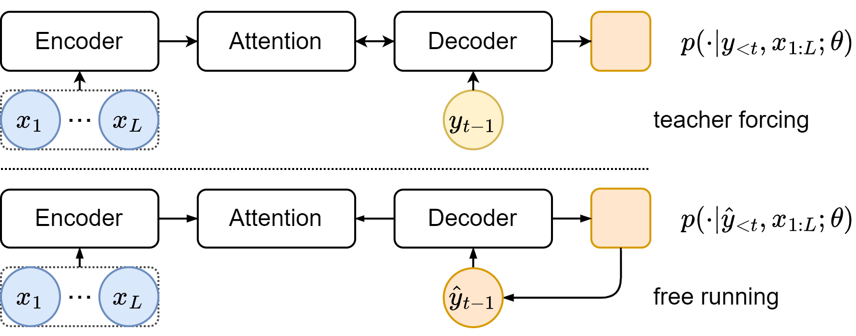
Figure 1: A general attention-based encoder-decoder model, operating in teacher forcing mode; a circle depicts a token, and a rounded square depicts a distribution.

2.2 Inference and training

During inference, given an input $\bm{x}_{1:L}$, the output $\hat{\bm{y}}_{1:T}$ can be obtained from the distribution estimated by the model $\bm{\theta}$:

$$\hat{\bm{y}}_{1:T}=\underset{\bm{y}_{1:T}}{\mathrm{argmax}}\,p(\bm{y}_{1:T}|\bm{x}_{1:L};\bm{\theta})$$ (3)

The exact search is often too expensive and is often approximated by greedy search for continuous output, or beam search for discrete output Bengio et al. (2015).

Conceptually, the model is trained to learn the natural distribution, e.g. through minimizing the KL-divergence between the natural distribution $p(\bm{y}_{1:T}|\bm{x}_{1:L})$ and the estimated distribution $p(\bm{y}_{1:T}|\bm{x}_{1:L};\bm{\theta})$. In practice, this can be approximated by minimizing the Negative Log-Likelihood (NLL) over some training data $\{\bm{y}^{(n)}_{1:T},\bm{x}^{(n)}_{1:L}\}_{1}^{N}$, sampled from the true distribution:

$$\mathcal{L}(\bm{\theta}) =\operatorname*{\mathbb{E}}_{\scalebox{0.8}{$\bm{x}_{1:L}$}}\mathrm{KL}\big{(}p(\bm{y}_{1:T}|\bm{x}_{1:L})||p(\bm{y}_{1:T}|\bm{x}_{1:L};\bm{\theta})\big{)}$$

$$\propto-\textstyle\sum_{n=1}^{N}\log p(\bm{y}^{(n)}_{1:T}|\bm{x}^{(n)}_{1:L};\bm{\theta})$$ (4)

$\mathcal{L}(\bm{\theta})$ denotes the loss. $N$ denotes the size of the training dataset; $n$ denotes the data index. To simplify the notation, the data index is omitted for the length of the sequences, although they also vary with the index. In the following sections, the sum over the training set $\sum_{n=1}^{N}$ will also be omitted.

For autoregressive models, and the sequence distribution $p(\bm{y}_{1:T}|\bm{x}_{1:L};\bm{\theta})$ is factorized across time, as shown in equation 1. A key question then, is how to compute the token distribution $p(\bm{y}_{t}|\bm{y}_{1:t-1},\bm{x}_{1:L};\bm{\theta})$. For teacher forcing, at each time step $t$, the token distribution is computed with the correct output history $\bm{y}_{1:t-1}$. In this case, the loss can be written as:

$$\begin{split}\mathcal{L}_{y}^{\tt T}(\bm{\theta})&=-\log p(\bm{y}_{1:T}|\bm{x}_{1:L};\bm{\theta})\\ &=-\textstyle\sum_{t=1}^{T}\log p(\bm{y}_{t}|\bm{y}_{1:t-1},\bm{x}_{1:L};\bm{\theta})\end{split}$$ (5)

From a theoretical point of view, this approach yields the correct model (zero KL-divergence) if the following assumptions hold: 1) the model is powerful enough ; 2) the model is optimized correctly; 3) there is enough training data to approximate the expectation shown in equation 4. In practice, these assumptions are often not true, hence the model is prone to mistakes. From a different perspective, teacher forcing suffers from exposure bias Ranzato et al. (2016), which refers to the following problem. During training, the model is guided by the reference output history. At the inference stage, however, the generated output history must be used. Hence there is a train-inference mismatch, and the errors accumulate along the inference process Ranzato et al. (2016).

Many approaches have been introduced to tackle exposure bias, and there are mainly two lines of research. Scheduled sampling Bengio et al. (2015); Duckworth et al. (2019) and professor forcing Lamb et al. (2016) are prominent examples along the first line. These approaches guide a model with both the reference and the generated output history, and the goal is to learn the data distribution via maximizing the likelihood of the training data. To facilitate convergence, they often depend on a heuristic schedule or an auxiliary classifier, which can be difficult to design and tune Bengio et al. (2015); Guo et al. (2019). The second line is a series of sequence-level training approaches, leveraging reinforcement learning Ranzato et al. (2016), minimum risk training Shen et al. (2016) or generative adversarial training Yu et al. (2017). Theses approaches guide a model with the generated output history. During training, the model operates in free running mode, and the goal is not to generate the reference output, but to optimize a sequence-level loss. However, many tasks do not have well established sequence-level objective metrics. Examples include speech synthesis, voice conversion, machine translation and text summarization Tay et al. (2020). Both lines of research require generating output sequences, and this process is sequential for autoregressive models. In recent years, models based on the Transformer Vaswani et al. (2017) have been widely used, and a key advantage is that when teacher forcing is used, training can be run in parallel across time. To efficiently generate output sequences from Transformer-based models, an approximation scheme Duckworth et al. (2019) has been proposed to parallelize scheduled sampling.

For the above training approaches, the model is trained at the token-level, i.e. the loss is computed for each token and summed across time. An alternative way of addressing exposure bias is to train the model at the sequence-level. Here the loss is computed for sequences instead of tokens, and the model sees not only the reference output during training. This type of approaches can be described in the framework of Minimum Bayes Risk (MBR) training. Assume that there is a distance metric $\mathcal{D}(\bm{y}_{1:T},\underline{\bm{y}}_{1:\underline{T}})$ between the reference output $\bm{y}_{1:T}$ and a random output $\underline{\bm{y}}_{1:\underline{T}}$, whose probability is estimated with the model $\bm{\theta}$. $\mathcal{D}$ is minimal when the two sequences are equal. MBR training minimizes its expected value:

$$\begin{split}\mathcal{L}_{y}^{\tt B}(\bm{\theta})&=\sum_{\underline{\bm{y}}_{1:\underline{T}}\in\mathcal{Y}}p(\underline{\bm{y}}_{1:\underline{T}}|\bm{x}_{1:L};\bm{\theta})\mathcal{D}(\bm{y}_{1:T},\underline{\bm{y}}_{1:\underline{T}})\end{split}$$ (6)

where $\mathcal{Y}$ is the entire output space.

3 Network Architecture

Deliberation networks are inspired by a common human behavior: when producing a sequence, be it text or speech, we often revise the initial output to improve its quality. For example, to write a good article, we usually first create a draft and then polish it. To record a section of an audio book, the readers often record several times until the quality is good enough.

A deliberation network consists of multiple models. Its output is generated in multiple passes, each one conditioned on the initial input and the previous free running output. With the iterative refinement, the final output is expected to be better than the previous ones. For deliberation networks, an essential element is to condition all but the first model on its previous free running output. This allows the later models to learn to correct the free running output, alleviating exposure bias. Without loss of generality, this section describes a two-pass deliberation network, shown in figure 2.

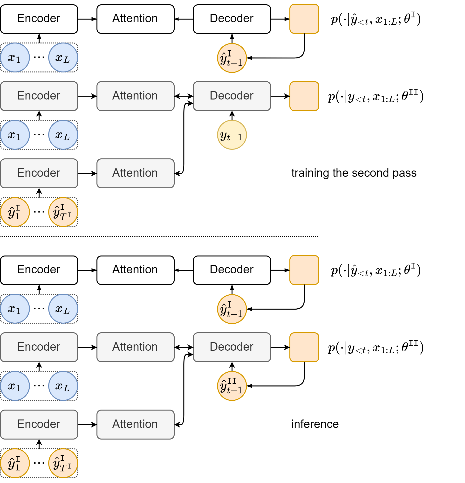
Figure 2: A two-pass deliberation network; the clear blocks depict the first pass; the shaded blocks depict the second pass.

In terms of notation, $\bm{x}_{1:L}$ and $\bm{y}_{1:T}$ denote the input and reference output; $\bm{\theta}^{\tt I}$ and $\bm{\theta}^{\tt II}$ denote the first-pass and second-pass models; $\bm{y}^{\tt I}_{1:T^{\tt I}}$ denotes an intermediate output sequence. The deliberation network models $p(\bm{y}_{1:T}|\bm{x}_{1:L})$ as

$$p(\bm{y}_{1:T}|\bm{x}_{1:L};\bm{\theta}^{\tt I},\bm{\theta}^{\tt II})=\textstyle\sum_{\bm{y}^{\tt I}_{1:T^{\tt I}}\in\mathcal{Y}}$$ (7)

$$p(\bm{y}^{\tt I}_{1:T^{\tt I}}|\bm{x}_{1:L};\bm{\theta}^{\tt I})p(\bm{y}_{1:T}|\bm{y}^{\tt I}_{1:T^{\tt I}},\bm{x}_{1:L};\bm{\theta}^{\tt II})$$

if $\bm{y}^{\tt I}_{1:T^{\tt I}}$ is discrete, and

$$p(\bm{y}_{1:T}|\bm{x}_{1:L};\bm{\theta}^{\tt I},\bm{\theta}^{\tt II})=\textstyle\int_{\bm{y}^{\tt I}_{1:T^{\tt I}}\in\mathcal{Y}}$$ (8)

$$p(\bm{y}^{\tt I}_{1:T^{\tt I}}|\bm{x}_{1:L};\bm{\theta}^{\tt I})p(\bm{y}_{1:T}|\bm{y}^{\tt I}_{1:T^{\tt I}},\bm{x}_{1:L};\bm{\theta}^{\tt II})d\bm{y}^{\tt I}_{1:T^{\tt I}}$$

if $\bm{y}^{\tt I}_{1:T^{\tt I}}$ is continuous. The summation/integration is over $\mathcal{Y}$, the entire space of $\bm{y}^{\tt I}_{1:T^{\tt I}}$. $p(\bm{y}^{\tt I}_{1:T^{\tt I}}|\bm{x}_{1:L};\bm{\theta}^{\tt I})$ is computed by $\bm{\theta}^{\tt I}$, a standard single-pass model. $p(\bm{y}_{1:T}|\bm{y}^{\tt I}_{1:T^{\tt I}},\bm{x}_{1:L};\bm{\theta}^{\tt II})$ is computed by $\bm{\theta}^{\tt II}$, a model with an additional attention mechanism over $\bm{y}^{\tt I}_{1:T^{\tt I}}$. $\bm{\theta}^{\tt I}$ and $\bm{\theta}^{\tt II}$ have different time steps. At time $t$, assuming $\bm{y}^{\tt I}_{1:T^{\tt I}}$ is available, $\bm{\theta}^{\tt II}$ operates as follows.

$$\bm{s}_{t}=f(\bm{y}_{1:t-1};\bm{\theta}_{s}^{\tt II})$$ (9)

$$\begin{split}\bm{h}_{x,1:L}=f(\bm{x}_{1:L};\bm{\theta}_{h,x}^{\tt II})\\ \bm{h}_{y,1:T^{\tt I}}=f(\bm{y}^{\tt I}_{1:T^{\tt I}};\bm{\theta}_{h,y}^{\tt II})\end{split}$$

$$\begin{split}\bm{\alpha}_{x,t}=f(\bm{s}_{t},\bm{h}_{x,1:L};\bm{\theta}_{\alpha,x}^{\tt II})\quad\bm{c}_{x,t}=\textstyle\sum_{l=1}^{L}\alpha_{x,t,l}\bm{h}_{x,l}\\ \bm{\alpha}_{y,t}=f(\bm{s}_{t},\bm{h}_{y,1:T^{\tt I}};\bm{\theta}_{\alpha,y}^{\tt II})\quad\bm{c}_{y,t}=\textstyle\sum_{l=1}^{T^{\tt I}}\alpha_{y,t,l}\bm{h}_{y,l}\end{split}$$

$$\hat{\bm{y}}_{t}^{\tt II}\sim p(\cdot|\bm{s}_{t},\bm{c}_{x,t},\bm{c}_{y,t};\bm{\theta}_{y}^{\tt II})$$

$\bm{\theta}^{\tt II}$ is built upon $\bm{\theta}^{\tt I}$, and has an additional encoder-attention pair. One pair $\{\bm{\theta}_{h,x}^{\tt II},\bm{\theta}_{\alpha,x}^{\tt II}\}$ is for the initial input $\bm{x}_{1:L}$; the additional pair $\{\bm{\theta}_{h,y}^{\tt II},\bm{\theta}_{\alpha,y}^{\tt II}\}$ is for the intermediate output $\bm{y}^{\tt I}_{1:T^{\tt I}}$. The encoder for $\bm{x}_{1:L}$ shares the same parameters as that of $\bm{\theta}^{\tt I}$, i.e. $\bm{\theta}_{h,x}^{\tt II}=\bm{\theta}_{h}^{\tt I}$. The probability of $\bm{y}_{t}$ depends on $\bm{s}_{t}$, $\bm{c}_{x,t}$ and $\bm{c}_{y,t}$. $\bm{s}_{t}$ is the state vector tracking the output history, and is used by both attention mechanisms. $\bm{c}_{x,t}$ and $\bm{c}_{y,t}$ summarize $\bm{x}_{1:L}$ and $\bm{y}^{\tt I}_{1:T^{\tt I}}$ respectively. The intermediate output of $\bm{\theta}^{\tt I}$, such as $\bm{s}^{\tt I}_{1:T^{\tt I}}$ and $\bm{c}^{\tt I}_{1:T^{\tt I}}$, can be combined with the $\bm{y}^{\tt I}_{1:T^{\tt I}}$ as the input to $\bm{\theta}_{h,y}^{\tt II}$.

During inference, the generated output history replaces the reference, and equation 9 becomes $\bm{s}_{t}=f(\hat{\bm{y}}_{1:t-1}^{\tt II};\bm{\theta}_{s}^{\tt II})$. The decoding of $\bm{\theta}^{\tt II}$ begins when that of $\bm{\theta}^{\tt I}$ is complete.

By default, the rest of this paper assumes that $\bm{y}^{\tt I}_{1:T^{\tt I}}$ is discrete, and most discussions are agnostic to the continuity of $\bm{y}^{\tt I}_{1:T^{\tt I}}$. When the continuity does make a difference, the discrete and continuous cases will be discussed separately.

4 Training

4.1 Joint Training

Table 1: Abbreviated expressions; these terms appear repeatedly in the equations, and are introduced to improve readability.

$F^{\tt I}$	$p(\bm{y}^{\tt I}_{1:T^{\tt I}}|\bm{x}_{1:L};\bm{\theta}^{\tt I})$
$F^{\tt II}$	$p(\bm{y}_{1:T}|\bm{y}^{\tt I}_{1:T^{\tt I}},\bm{x}_{1:L};\bm{\theta}^{\tt II})$
$\hat{F}^{{\tt I}(m)}$	$p(\hat{\bm{y}}^{{\tt I}(m)}_{1:T^{{\tt I}(m)}}|\bm{x}_{1:L};\bm{\theta}^{\tt I})$
$\hat{F}^{{\tt II}(m)}$	$p(\bm{y}_{1:T}|\hat{\bm{y}}^{{\tt I}(m)}_{1:T^{{\tt I}(m)}},\bm{x}_{1:L};\bm{\theta}^{\tt II})$

In theory, ${\bm{\theta}}^{\tt I}$ and ${\bm{\theta}}^{\tt II}$ can be trained by directly maximizing the log of the likelihood in equation 7, and the loss function $\check{\mathcal{L}}_{y}$ is

$$\check{\mathcal{L}}_{y}(\bm{\theta}^{\tt I},\bm{\theta}^{\tt II}) =-\log p(\bm{y}_{1:T}|\bm{x}_{1:L};\bm{\theta}^{\tt I},\bm{\theta}^{\tt II})$$ (10)

$$=-\log\textstyle\sum_{\bm{y}^{\tt I}_{1:T^{\tt I}}\in\mathcal{Y}}F^{\tt I}F^{\tt II}$$

$F^{\tt I}$ and $F^{\tt II}$ are abbreviated expressions defined in table 1. As discussed in section 2.2, if $\check{\mathcal{L}}_{y}$ were fully optimized, the KL-divergence between the model distribution $p(\bm{y}_{1:T}|\bm{x}_{1:L};\bm{\theta}^{\tt I},\bm{\theta}^{\tt II})$ and the true distribution $p(\bm{y}_{1:T}|\bm{x}_{1:L})$ would be zero. In general, the actual divergence is limited by the model, data and training. In particular, for deliberation networks, the sum over $\bm{y}^{\tt I}_{1:T^{\tt I}}$ is intractable due to the prohibitively large space of $\bm{y}^{\tt I}_{1:T^{\tt I}}$. A Monte Carlo estimator is often used to approximate either the loss or the gradients. The gradients of $\check{\mathcal{L}}_{y}$ w.r.t the model parameters $\bm{\theta}^{\tt I}$ and $\bm{\theta}^{\tt II}$ are

$$\triangledown_{\bm{\theta}^{\tt I}}\check{\mathcal{L}}_{y}(\bm{\theta}^{\tt I},\bm{\theta}^{\tt II})=-\displaystyle\frac{{\sum_{\bm{y}^{\tt I}_{1:T^{\tt I}}\in\mathcal{Y}}}F^{\tt II}(\triangledown_{\bm{\theta}^{\tt I}}F^{\tt I})}{\sum_{\bm{y}^{\tt I}_{1:T^{\tt I}}\in\mathcal{Y}}F^{\tt I}F^{\tt II}}$$ (11)

$$\triangledown_{\bm{\theta}^{\tt II}}\check{\mathcal{L}}_{y}(\bm{\theta}^{\tt I},\bm{\theta}^{\tt II})=-\displaystyle\frac{{\sum_{\bm{y}^{\tt I}_{1:T^{\tt I}}\in\mathcal{Y}}}F^{\tt I}(\triangledown_{\bm{\theta}^{\tt II}}F^{\tt II})}{\sum_{\bm{y}^{\tt I}_{1:T^{\tt I}}\in\mathcal{Y}}F^{\tt I}F^{\tt II}}$$ (12)

The sum over the output space appears twice in equations 11 and 12, which makes the gradient computation more difficult than necessary. A commonly used technique is to instead minimize an upper bound $\mathcal{L}_{y}$ Xia et al. (2017):

$$\mathcal{L}_{y}(\bm{\theta}^{\tt I},\bm{\theta}^{\tt II}) =-\textstyle\sum_{\bm{y}^{\tt I}_{1:T^{\tt I}}\in\mathcal{Y}}F^{\tt I}\log F^{\tt II}$$ (13)

$$\geq\check{\mathcal{L}}_{y}(\bm{\theta}^{\tt I},\bm{\theta}^{\tt II})$$

The upper bound is derived with the concavity of the log function and the fact that $\sum_{\bm{y}^{\tt I}_{1:T^{\tt I}}\in\mathcal{Y}}p(\bm{y}^{\tt I}_{1:T^{\tt I}}|\bm{x}_{1:L};\bm{\theta}^{\tt I})=1$. The gradients of $\mathcal{L}_{y}$ w.r.t. $\bm{\theta}^{\tt I}$ and $\bm{\theta}^{\tt II}$ are

$$\triangledown_{\bm{\theta}^{\tt I}}\mathcal{L}_{y}(\bm{\theta}^{\tt I},\bm{\theta}^{\tt II})=$$ (14)

$$-\textstyle\sum_{\bm{y}^{\tt I}_{1:T^{\tt I}}\in\mathcal{Y}}F^{\tt I}(\log F^{\tt II})(\triangledown_{\bm{\theta}^{\tt I}}\log F^{\tt I})$$

$$\triangledown_{\bm{\theta}^{\tt II}}\mathcal{L}_{y}(\bm{\theta}^{\tt I},\bm{\theta}^{\tt II})=$$ (15)

$$-\textstyle\sum_{\bm{y}^{\tt I}_{1:T^{\tt I}}\in\mathcal{Y}}F^{\tt I}(\triangledown_{\bm{\theta}^{\tt II}}\log F^{\tt II})$$

Equation 14 is derived using the identity $\triangledown_{\bm{\theta}}f(\bm{\theta})=f(\bm{\theta})\triangledown_{\bm{\theta}}\log f(\bm{\theta})$. Compared with the previous gradients shown in equations 11 and 12, the new gradients, $\triangledown_{\bm{\theta}^{\tt I}}\mathcal{L}_{y}$ and $\triangledown_{\bm{\theta}^{\tt II}}\mathcal{L}_{y}$, are simpler in the sense that the summation over the output space appears only once.

Comparing equations 13 and 6, it can be seen that for $\bm{\theta}^{\tt I}$, the loss fits into the framework of Minimum Bayes Risk (MBR) training, described in section 2.2. Here the risk is defined as $-\log p(\bm{y}_{1:T}|\bm{y}^{{\tt I}}_{1:T^{{\tt I}}},\bm{x}_{1:L};\bm{\theta}^{\tt II})$. The following subsections will describe two ways of using Monte Carlo approximation, in order to approximate the summation over the output space. They differ in whether to approximate the loss or the gradient, but they can adopt the same sampling process.

4.1.1 Approximating Gradients

Applying Monte Carlo approximation, the gradients $\triangledown_{\bm{\theta}^{\tt I}}\mathcal{L}_{y}$ and $\triangledown_{\bm{\theta}^{\tt II}}\mathcal{L}_{y}$ are estimated as

$$\triangledown_{\bm{\theta}^{\tt I}}\mathcal{L}_{y}(\bm{\theta}^{\tt I},\bm{\theta}^{\tt II})\approx$$ (16)

$$-\textstyle\frac{1}{M}\sum_{m=1}^{M}(\log\hat{F}^{{\tt II}(m)})(\triangledown_{\bm{\theta}^{\tt I}}\log\hat{F}^{{\tt I}(m)})$$

$$\triangledown_{\bm{\theta}^{\tt II}}\mathcal{L}_{y}(\bm{\theta}^{\tt I},\bm{\theta}^{\tt II})\approx$$ (17)

$$-\textstyle\frac{1}{M}\sum_{m=1}^{M}\triangledown_{\bm{\theta}^{\tt II}}\log\hat{F}^{{\tt II}(m)}$$

$\hat{F}^{{\tt I}(m)}$ and $\hat{F}^{{\tt II}(m)}$ are abbreviated expressions defined in table 1. $\{\hat{\bm{y}}^{{\tt I}(1)}_{1:T^{{\tt I}(1)}},...,\hat{\bm{y}}^{{\tt I}(M)}_{1:T^{{\tt I}(M)}}\}$ are $M$ i.i.d. samples drawn from the distribution $p(\bm{y}^{\tt I}_{1:T^{\tt I}}|\bm{x}_{1:L};\bm{\theta}^{\tt I})$. The Monte Carlo estimator is unbiased, and its variance is proportional to $\frac{1}{M}$. There is a trade-off between the variance and the computational cost: fewer samples results in higher variance, but lower cost. For SGD-based optimization, noisy estimates of the gradients are used, and this variance adds another level of noise.

The sampling process is often realized by beam search or (a noisy version of) greedy search Prabhavalkar et al. (2018), as described in section 2.2. Once the sampling process is complete, $\triangledown_{\bm{\theta}^{\tt I}}\mathcal{L}_{y}$ and $\triangledown_{\bm{\theta}^{\tt II}}\mathcal{L}_{y}$ can be computed. For $\bm{\theta}^{\tt I}$, the training is equivalent to MBR training. For $\bm{\theta}^{\tt II}$, the training can be viewed as teacher forcing, because to compute the conditional probability of the reference output, the reference back-history is used.

4.1.2 Approximating Loss

Alternatively, Monte Carlo approximation can be applied to the loss $\mathcal{L}_{y}$ shown in equation 13, before deriving the gradients. Let $\bar{\mathcal{L}}_{y}$ denote the approximation:

$$\mathcal{L}_{y}(\bm{\theta}^{\tt I},\bm{\theta}^{\tt II})\approx\bar{\mathcal{L}}_{y}(\bm{\theta}^{\tt I},\bm{\theta}^{\tt II})$$ (18)

$$=\textstyle-\frac{1}{M}\sum_{m=1}^{M}\log p(\bm{y}_{1:T}|\hat{\bm{y}}^{{\tt I}(m)}_{1:T^{{\tt I}(m)}},\bm{x}_{1:L};\bm{\theta}^{\tt II})$$

It is simple to compute $\triangledown_{\bm{\theta}^{\tt II}}\bar{\mathcal{L}}_{y}$. However, computing $\triangledown_{\bm{\theta}^{\tt I}}\bar{\mathcal{L}}_{y}$ is not trivial, because it requires differentiating through $\hat{\bm{y}}^{{\tt I}(m)}_{1:T^{{\tt I}(m)}}$, a random sample drawn from a distribution. The sampling process can be formulated as a deterministic function of $\bm{\theta}^{\tt I}$, using reparameterization tricks, such as Gumbel softmax Jang et al. (2017). In general, suppose $\bm{y}^{\tt I}_{1:T^{\tt I}}$ can be viewed as a function of a random variable $\bm{z}$, and drawing samples from its distribution $p(\bm{z})$ is practical. Then instead of drawing $\{\hat{\bm{y}}^{{\tt I}(1)}_{1:T^{{\tt I}(1)}},...,\hat{\bm{y}}^{{\tt I}(M)}_{1:T^{{\tt I}(M)}}\}$ from $p(\bm{y}^{\tt I}_{1:T^{\tt I}}|\bm{x}_{1:L};\bm{\theta}^{\tt I})$, we can draw $\{\hat{\bm{z}}^{(1)},...,\hat{\bm{z}}^{(M)}\}$ from $p(\bm{z})$:

$$\hat{\bm{z}}^{(m)}\sim p(\bm{z});\;\hat{\bm{y}}^{{\tt I}(m)}_{1:T^{{\tt I}(m)}}=f(\hat{\bm{z}}^{(m)},\bm{x}_{1:L};\bm{\theta}^{\tt I})$$ (19)

The gradients for $\bm{\theta}^{\tt I}$ and $\bm{\theta}^{\tt II}$ are

$$\triangledown_{\bm{\theta}^{\tt I}}\bar{\mathcal{L}}_{y}(\bm{\theta}^{\tt I},\bm{\theta}^{\tt II})\approx$$ (20)

$$\textstyle-\frac{1}{M}\sum_{m=1}^{M}(\triangledown_{\hat{\bm{y}}^{{\tt I}(m)}_{1:T^{{\tt I}(m)}}}\log\hat{F}^{{\tt II}(m)})(\triangledown_{\bm{\theta}^{\tt I}}\hat{\bm{y}}^{{\tt I}(m)}_{1:T^{{\tt I}(m)}})$$

$$\triangledown_{\bm{\theta}^{\tt II}}\bar{\mathcal{L}}_{y}(\bm{\theta}^{\tt I},\bm{\theta}^{\tt II})\approx$$ (21)

$$\textstyle-\frac{1}{M}\sum_{m=1}^{M}\triangledown_{\bm{\theta}^{\tt II}}\log\hat{F}^{{\tt II}(m)}$$

Note that $\bm{y}^{\tt I}_{1:T^{\tt I}}$ is independent of $\bm{\theta}^{\tt I}$, and the summation in equation 10 is over the entire space of $\bm{y}^{\tt I}_{1:T^{\tt I}}$. Hence $\triangledown_{\bm{\theta}^{\tt I}}p(\bm{y}_{1:T}|\bm{y}^{\tt I}_{1:T^{\tt I}},\bm{x}_{1:L};\bm{\theta}^{\tt II})=0$, and equations 14 and 16 hold. In contrast, $\hat{\bm{y}}^{{\tt I}(m)}_{1:T^{{\tt I}(m)}}$ depends on $\bm{\theta}^{\tt I}$, and the summation in equation 18 is over a set depending on $\bm{\theta}^{\tt I}$. $\hat{\bm{y}}^{{\tt I}(m)}_{1:T^{{\tt I}(m)}}$ can be viewed as a deterministic function of $\bm{\theta}^{\tt I}$. Hence $\triangledown_{\bm{\theta}^{\tt I}}p(\bm{y}_{1:T}|\hat{\bm{y}}^{{\tt I}(m)}_{1:T^{{\tt I}(m)}},\bm{x}_{1:L};\bm{\theta}^{\tt II})\neq 0$, and equation 20 holds.

For the second-pass model $\bm{\theta}^{\tt II}$, given the same group of samples, the gradients remain the same, i.e. $\triangledown_{\bm{\theta}^{\tt II}}\mathcal{L}_{y}=\triangledown_{\bm{\theta}^{\tt II}}\bar{\mathcal{L}}_{y}$, whether Monte Carlo approximation is applied to the loss or the gradients. For the first-pass model $\bm{\theta}^{\tt I}$, unless $M\to+\infty$, the gradients $\triangledown_{\bm{\theta}^{\tt I}}\mathcal{L}_{y}$ and $\triangledown_{\bm{\theta}^{\tt I}}\bar{\mathcal{L}}_{y}$ are usually different. It is not trivial to mathematically characterize the difference. However, from a practical point of view, it is simpler to apply Monte Carlo approximation to the gradients, which does not require any reparameterization trick. This explains why applying Monte Carlo approximation to the gradients is more common in existing research Xia et al. (2017); Hu et al. (2020).

The joint training scheme has several drawbacks. As there is no loss over the intermediate output $\hat{\bm{y}}^{{\tt I}(m)}_{1:T^{{\tt I}(m)}}$, it is likely to deviate from valid target sequences. This makes it difficult to analyze the system. More importantly, if $\bm{\theta}^{\tt I}$ is randomly initialized, the intermediate output will be close to random noise, making it difficult for $\bm{\theta}^{\tt II}$ to learn to refine the intermediate output. In practice, it is common to pretrain $\bm{\theta}^{\tt I}$ with teacher forcing, in order to address these problems Hu et al. (2020).

In terms of efficiency, one important problem is that the sampling process is very often auto-regressive, in which case joint training cannot be run in parallel. Recently, Transformer-style models are widely used in various seq2seq tasks. One of their main advantages is parallel training. If teacher forcing is used, there is no recurrent connection in the model, and training can be done in parallel across the length $T$ of the output $\bm{y}_{1:T}$, because the reference output history $\bm{y}_{1:t-1}$ is available for any $t$. However, if sampling is required, these models must operate sequentially, because the generated output history $\hat{\bm{y}}_{1:t-1}$ must be used, which is not available beforehand.

4.2 Separate Training

For separate training, $\bm{\theta}^{\tt I}$ is trained as a standard sequence-to-sequence model with teacher forcing:

$$\mathcal{L}_{y}(\bm{\theta}^{\tt I}) =-\log p(\bm{y}_{1:T}|\bm{x}_{1:L};\bm{\theta}^{\tt I})$$ (22)

Then it is fixed to generate samples $\{\hat{\bm{y}}^{{\tt I}(1)}_{1:T^{{\tt I}(1)}},...,\hat{\bm{y}}^{{\tt I}(M)}_{1:T^{{\tt I}(M)}}\}$ for each input $\bm{x}_{1:L}$, using beam search or (a noisy version of) greedy search. Next, $\bm{\theta}^{\tt II}$ is again trained with teacher forcing:

$$\mathcal{L}_{y}(\bm{\theta}^{\tt II}) =-\log\textstyle\frac{1}{M}\sum_{m=1}^{M}\hat{F}^{{\tt II}(m)}$$ (23)

The gradients for $\bm{\theta}^{\tt I}$ and $\bm{\theta}^{\tt I}$ are

$$\triangledown_{\bm{\theta}^{\tt I}}\mathcal{L}_{y}(\bm{\theta}^{\tt I})=\textstyle-\triangledown_{\bm{\theta}^{\tt I}}\log p(\bm{y}_{1:T}|\bm{x}_{1:L};\bm{\theta}^{\tt I})$$ (24)

$$\triangledown_{\bm{\theta}^{\tt II}}\mathcal{L}_{y}(\bm{\theta}^{\tt II})=\textstyle-\frac{1}{M}\sum_{m=1}^{M}\triangledown_{\bm{\theta}^{\tt II}}\log\hat{F}^{{\tt II}(m)}$$ (25)

For $\bm{\theta}^{\tt II}$, the gradient is the same for separate training and joint training, given the same group of samples. This can be seen by comparing equations 17 and 25. For $\bm{\theta}^{\tt I}$, however, there is a major difference. As described in the previous subsection, joint training uses a noisy Monte Carlo estimator for either the loss or the gradient, and is empirically found to be unstable Xia et al. (2017). In contrast, for separate training, $\bm{\theta}^{\tt I}$ is trained with teacher forcing, and is free from the above problem. This can be seen by comparing equation 24 to equations 16 and 20.

The separate training approach has the advantage that it allows parallel training. As $\bm{\theta}^{\tt I}$ is fixed, the sample $\hat{\bm{y}}^{\tt I}_{1:T^{\tt I}}$ can be generated and stored beforehand. So that when predicting $\bm{y}_{t}$, all the required information is available, including $\bm{x}_{1:L}$, $\bm{y}_{1:t-1}$ and $\hat{\bm{y}}^{\tt I}_{1:T^{\tt I}}$.

4.3 Discussion

For all the approaches described above, there is a common choice: when updating the parameters of the second-pass model $\bm{\theta}^{\tt II}$, the first-pass model $\bm{\theta}^{\tt I}$ runs in free running mode. In other words, during training, the output $\hat{\bm{y}}^{{\tt I}}_{1:T^{{\tt I}}}$ from $\bm{\theta}^{\tt I}$ is generated in free running mode, instead of teacher forcing mode. This trains $\bm{\theta}^{\tt II}$ to fix the errors made by $\bm{\theta}^{\tt I}$ in free running mode, i.e. to address exposure bias. Empirically, it is shown that if the $\bm{\theta}^{\tt I}$ runs in teacher forcing mode while $\bm{\theta}^{\tt II}$ is trained, the network will not have any performance gain at the inference stage Dou et al. (2021b).

Intuitively, when computing the distribution of $\bm{y}_{1:T}$, knowing $\hat{\bm{y}}^{{\tt I}}_{1:T^{{\tt I}}}$ leads to some information gain. This can be quantified by mutual information between $\bm{y}_{1:T}$ and $\hat{\bm{y}}^{{\tt I}}_{1:T^{{\tt I}}}$. Assuming that the expectation over the intermediate output is approximated by a single sample, the information gain can be formulated as:

$$\mathcal{G}(\bm{y}_{1:T},\hat{\bm{y}}^{{\tt I}}_{1:T^{{\tt I}}}) =\textstyle\frac{1}{T}\sum_{t=1}^{T}\mathcal{H}(p(\bm{y}_{t}|\bm{y}_{<t};\bm{\theta}^{\tt I}))-$$

$$\mathcal{H}(p(\bm{y}_{t}|\bm{y}_{<t},\hat{\bm{y}}^{{\tt I}}_{1:T^{{\tt I}}};\bm{\theta}^{\tt I},\bm{\theta}^{\tt II}))$$ (26)

Here the input sequence is omitted for simplicity. $\mathcal{G}(\bm{y}_{1:T},\hat{\bm{y}}^{{\tt I}}_{1:T^{{\tt I}}})$ denotes the information gain from condition the distribution of $\bm{y}_{1:T}$ on $\hat{\bm{y}}^{{\tt I}}_{1:T^{{\tt I}}}$. The intermediate output sequence is generated in free running mode, and is denoted $\hat{\bm{y}}^{{\tt I}}_{1:T^{{\tt I}}}$. Alternatively, the output sequence can be generated in teacher forcing mode. Let $\check{\bm{y}}^{{\tt I}}_{1:T^{{\tt I}}}$ the alternative sequence, the information gain becomes:

$$\mathcal{G}(\bm{y}_{1:T},\check{\bm{y}}^{{\tt I}}_{1:T^{{\tt I}}}) =\textstyle\frac{1}{T}\sum_{t=1}^{T}\mathcal{H}(p(\bm{y}_{t}|\bm{y}_{<t};\bm{\theta}^{\tt I}))-$$

$$\mathcal{H}(p(\bm{y}_{t}|\bm{y}_{<t},\check{\bm{y}}^{{\tt I}}_{1:T^{{\tt I}}};\bm{\theta}^{\tt I},\bm{\theta}^{\tt II}))$$ (27)

We hypothesize that $\mathcal{G}(\bm{y}_{1:T},\check{\bm{y}}^{{\tt I}}_{1:T^{{\tt I}}})\leq\mathcal{G}(\bm{y}_{1:T},\hat{\bm{y}}^{{\tt I}}_{1:T^{{\tt I}}})$, because the teacher forcing sequence is very similar to the reference sequence $\bm{y}_{1:T}$, and adds less information than the free running sequence. Experiments will be conducted in our future work to test this hypothesis.

So far in this section, it has been assumed that the goal of training is to learn a natural distribution. There are alternative options. For example, the entire network can be trained with MBR training, as described in section 2.2. This is often adopted in tasks with a gold-standard objective metric, e.g. word error rate for ASR Hu et al. (2020, 2021). While this work focuses on supervised training, deliberation networks can also be used in unsupervised training. For example, a cycle consistency loss can be used in tasks where there is not a lot of paired data, such as image-to-image translation and voice conversion He et al. (2019a).

5 Application Considerations

When applying deliberation networks, it is essential to consider the nature of the input and the output. There are two key factors to consider. The first is whether the input and output have the same continuity. If so, they can be embedded in the same way. Examples include NMT and voice conversion. More precisely speaking, the initial input $\bm{x}_{1:L}$ and the first-pass output $\bm{y}^{\tt I}_{1:T^{\tt I}}$ are either both continuous or both discrete. Hence the additional encoder and attention mechanism for the first-pass output, $\bm{\theta}_{h,y}^{\tt II}$ and $\bm{\theta}_{\alpha,y}^{\tt II}$, can have exactly the same structure as those for the initial input, $\bm{\theta}_{h,x}^{\tt II}$ and $\bm{\theta}_{\alpha,x}^{\tt II}$. When the input and output are different in terms of continuity, the additional encoder needs to be modified. For example, for TTS, $\bm{x}_{1:L}$ is a discrete text sequence, and $\bm{y}^{\tt I}_{1:T^{\tt I}}$ is a continuous speech sequence. Here the text embedding layer in $\bm{\theta}_{h,x}^{\tt II}$ can be replaced by a linear layer in $\bm{\theta}_{h,y}^{\tt II}$. The second key factor to consider is whether the output is naturally discrete or continuous. The rest of this section will discuss both cases.

5.1 Discrete output

On a historical note, deliberation networks were first introduced for sequence-to-sequences tasks where both the input and output are text, such as NMT Xia et al. (2017). Their application was later extended to ASR, where the input is audio and the output is text. For these tasks, the additional attention connects two text sequences, which are naturally discrete. Compared with audio sequences, which are naturally continuous, text sequences are usually shorter and the tokens are less correlated in time. Therefore, it is easier for the additional attention to learn to align the sequences, and the standard training approaches in section 4 work out-of-the-box Hu et al. (2020); Dou (2022).

When it comes to ASR, streaming is an increasingly important demand Hu et al. (2020, 2021); Mavandadi et al. (2021). Typically, the first-pass model is a streaming model such as RNN-Transducer (RNN-T) He et al. (2019b), and the RNN-T loss for the first-pass model is combined with the likelihood loss for the second-pass model, described in section 4. In some cases, MBR training is also applied to the second-pass model, directly optimizing the word error rate Hu et al. (2020, 2021). To improve the streaming outputs, the second-pass model often adopts more powerful building blocks, such as Transformer blocks. The most common training scheme is separate training followed by joint training. During joint training, the first-pass model generates samples sequentially, but this is less problematic than the other application cases, thanks to the efficiency of the first-pass model.

5.2 Continuous output

Continuous sequences, such as audio, are usually longer than discrete sequences, such as text. In general, longer sequences are harder for the attention mechanism, and reducing the time resolution alleviates the problem. For example, a pyramid encoder is often used in attention-based ASR models Chan et al. (2016). Alternatively, when applying deliberation networks to TTS, adjacent frames in the first-pass output $\bm{y}^{\tt I}_{1:T^{\tt I}}$ can be stacked in groups, forming a shorter sequence, before being fed into the encoder Dou et al. (2021b).

Another challenge for continuous sequences is the strong correlation across time, i.e. among the tokens, which makes it hard to find the right tokens to focus on. For deliberation networks, the second-pass model has two sources of information: the initial input sequence $\bm{x}_{1:L}$ and the first-pass output $\bm{y}^{\tt I}_{1:T^{\tt I}}$. When $\bm{y}^{\tt I}_{1:T^{\tt I}}$ is continuous, the second-pass model is likely to ignore $\bm{y}^{\tt I}_{1:T^{\tt I}}$, as learning to attend to $\bm{x}_{1:L}$ can be enough for reaching a local optimum during training. In this case, the attention over $\bm{x}_{1:L}$ does not produce any meaningful alignment, and the deliberation network degrades into a standard single-pass model. To tackle this issue, the attention can be regularized. This is relatively simple when the attention is expected to be monotonic. For example, when applying deliberation networks to TTS, a guided attention loss Tachibana et al. (2018) can be added:

$$\begin{split}&\mathcal{L}_{\alpha}(\bm{\theta}^{\tt II})=\textstyle\sum_{t=1}^{T}\sum_{l=1}^{T^{\tt I}}[\alpha_{y,t,l}w_{t,l}]\\ &w_{t,l}=1-\exp{(-(t/T-l/T^{\tt I})/2g^{2})}\end{split}$$ (28)

where $g$ is a hyperparameter controlling the sharpness, and $\alpha_{y,t,l}$ is an element of the attention map $\bm{\alpha}_{y,1:T}$. This encourages $\bm{\alpha}_{y,1:T}$ to be diagonal, enabling $\bm{\theta}^{\tt II}$ to make more extensive use of $\bm{y}^{\tt I}_{1:T^{\tt I}}$. For $\bm{\theta}^{\tt II}$, the complete loss is

$$\mathcal{L}_{y,\alpha}(\bm{\theta}^{\tt II})=\mathcal{L}_{y}(\bm{\theta}^{\tt II})+\gamma\mathcal{L}_{\alpha}(\bm{\theta}^{\tt II})$$ (29)

where $\gamma$ is a scaling factor. When $\mathcal{L}_{\alpha}$ is used, it is important to monitor $\bm{\alpha}_{y,1:T}$ and the inference performance on a validation set via objective metrics such as Global Variance Dou et al. (2021b). When $\bm{\alpha}_{y,1:T}$ is sharply diagonal, $\mathcal{L}_{\alpha}$ is low, but the inference performance may degrade.

6 Conclusion

This paper introduces a unifying framework for deliberation networks, investigating various training options and application considerations. The key insights are as follows. First, to deal with the intractable marginalization of the intermediate output, it is simpler to apply Monte Carlo approximation to the gradients instead of the loss. Second, parallel training is possible for deliberation networks, as long as each pass is trained separately. Third, regardless of the application, it is essential that when training the parameters of a certain pass, its previous pass runs in free running mode. Finally, for applications where the output is continuous, a guided attention loss can be used to prevent the multi-pass model from degrading into a single-pass model.

References

- Bengio et al. (2015) Samy Bengio, Oriol Vinyals, Navdeep Jaitly, and Noam Shazeer. 2015. Scheduled sampling for sequence prediction with recurrent neural networks. In Advances in Neural Information Processing Systems, pages 1171–1179.
- Chan et al. (2016) William Chan, Navdeep Jaitly, Quoc V Le, and Oriol Vinyals. 2016. Listen, attend and spell: A neural network for large vocabulary conversational speech recognition. 2016 IEEE International Conference on Acoustics, Speech and Signal Processing (ICASSP).
- Dou (2022) Qingyun Dou. 2022. Improving Attention-based Sequence-to-sequence Models. Ph.D. thesis, University of Cambridge.
- Dou et al. (2020) Qingyun Dou, Joshua Efiong, and Mark JF Gales. 2020. Attention forcing for speech synthesis. Proc. Interspeech 2020, pages 4014–4018.
- Dou et al. (2021a) Qingyun Dou, Yiting Lu, Potsawee Manakul, Xixin Wu, and Mark J. F. Gales. 2021a. Attention forcing for machine translation. arXiv preprint arXiv:2104.01264.
- Dou et al. (2021b) Qingyun Dou, Xixin Wu, Moquan Wan, Yiting Lu, and Mark JF Gales. 2021b. Deliberation-based multi-pass speech synthesis. In Interspeech, pages 136–140.
- Duckworth et al. (2019) Daniel Duckworth, Arvind Neelakantan, Ben Goodrich, Lukasz Kaiser, and Samy Bengio. 2019. Parallel scheduled sampling. arXiv preprint arXiv:1906.04331.
- Guo et al. (2019) Haohan Guo, Frank K Soong, Lei He, and Lei Xie. 2019. A new GAN-based end-to-end TTS training algorithm. Interspeech.
- He et al. (2019a) Tianyu He, Yingce Xia, Jianxin Lin, Xu Tan, Di He, Tao Qin, and Zhibo Chen. 2019a. Deliberation learning for image-to-image translation. In IJCAI, pages 2484–2490.
- He et al. (2019b) Yanzhang He, Tara N Sainath, Rohit Prabhavalkar, Ian McGraw, Raziel Alvarez, Ding Zhao, David Rybach, Anjuli Kannan, Yonghui Wu, Ruoming Pang, et al. 2019b. Streaming end-to-end speech recognition for mobile devices. In ICASSP 2019-2019 IEEE International Conference on Acoustics, Speech and Signal Processing (ICASSP), pages 6381–6385. IEEE.
- Hu et al. (2021) Ke Hu, Ruoming Pang, Tara N Sainath, and Trevor Strohman. 2021. Transformer based deliberation for two-pass speech recognition. In 2021 IEEE Spoken Language Technology Workshop (SLT), pages 68–74. IEEE.
- Hu et al. (2020) Ke Hu, Tara N Sainath, Ruoming Pang, and Rohit Prabhavalkar. 2020. Deliberation model based two-pass end-to-end speech recognition. In ICASSP 2020-2020 IEEE International Conference on Acoustics, Speech and Signal Processing (ICASSP), pages 7799–7803. IEEE.
- Huang et al. (2016) Po-Yao Huang, Frederick Liu, Sz-Rung Shiang, Jean Oh, and Chris Dyer. 2016. Attention-based multimodal neural machine translation. In Proceedings of the First Conference on Machine Translation: Volume 2, Shared Task Papers, pages 639–645.
- Jang et al. (2017) Eric Jang, Shixiang Gu, and Ben Poole. 2017. Categorical reparameterization with Gumbel-softmax. stat, 1050:5.
- Lamb et al. (2016) Alex M Lamb, Anirudh Goyal Alias Parth Goyal, Ying Zhang, Saizheng Zhang, Aaron C Courville, and Yoshua Bengio. 2016. Professor forcing: A new algorithm for training recurrent networks. In Advances In Neural Information Processing Systems, pages 4601–4609.
- Lewis et al. (2020) Mike Lewis, Yinhan Liu, Naman Goyal, Marjan Ghazvininejad, Abdelrahman Mohamed, Omer Levy, Veselin Stoyanov, and Luke Zettlemoyer. 2020. BART: Denoising sequence-to-sequence pre-training for natural language generation, translation, and comprehension. In Proceedings of the 58th Annual Meeting of the Association for Computational Linguistics, pages 7871–7880.
- Mavandadi et al. (2021) Sepand Mavandadi, Tara N Sainath, Kevin Hu, and Zelin Wu. 2021. A deliberation-based joint acoustic and text decoder. In Proc. Interspeech 2021.
- Neubig (2017) Graham Neubig. 2017. Neural machine translation and sequence-to-sequence models: A tutorial. arXiv preprint arXiv:1703.01619.
- Prabhavalkar et al. (2018) Rohit Prabhavalkar, Tara N Sainath, Yonghui Wu, Patrick Nguyen, Zhifeng Chen, Chung-Cheng Chiu, and Anjuli Kannan. 2018. Minimum word error rate training for attention-based sequence-to-sequence models. In 2018 IEEE International Conference on Acoustics, Speech and Signal Processing (ICASSP), pages 4839–4843. IEEE.
- Ranzato et al. (2016) Marc’Aurelio Ranzato, Sumit Chopra, Michael Auli, and Wojciech Zaremba. 2016. Sequence level training with recurrent neural networks. In 4th International Conference on Learning Representations, ICLR.
- Shen et al. (2018) Jonathan Shen, Ruoming Pang, Ron J Weiss, Mike Schuster, Navdeep Jaitly, Zongheng Yang, Zhifeng Chen, Yu Zhang, Yuxuan Wang, Rj Skerrv-Ryan, et al. 2018. Natural TTS synthesis by conditioning WaveNet on mel spectrogram predictions. In 2018 IEEE International Conference on Acoustics, Speech and Signal Processing (ICASSP), pages 4779–4783. IEEE.
- Shen et al. (2016) Shiqi Shen, Yong Cheng, Zhongjun He, Wei He, Hua Wu, Maosong Sun, and Yang Liu. 2016. Minimum risk training for neural machine translation. In Proceedings of the 54th Annual Meeting of the Association for Computational Linguistics (Volume 1: Long Papers), pages 1683–1692.
- Tachibana et al. (2018) Hideyuki Tachibana, Katsuya Uenoyama, and Shunsuke Aihara. 2018. Efficiently trainable text-to-speech system based on deep convolutional networks with guided attention. In 2018 IEEE International Conference on Acoustics, Speech and Signal Processing (ICASSP), pages 4784–4788. IEEE.
- Tay et al. (2020) Yi Tay, Mostafa Dehghani, Dara Bahri, and Donald Metzler. 2020. Efficient Transformers: A survey. arXiv preprint arXiv:2009.06732.
- Vaswani et al. (2017) Ashish Vaswani, Noam Shazeer, Niki Parmar, Jakob Uszkoreit, Llion Jones, Aidan N Gomez, Lukasz Kaiser, and Illia Polosukhin. 2017. Attention is all you need. Advances in Neural Information Processing Systems.
- Wang et al. (2018) Yuxuan Wang, Daisy Stanton, Yu Zhang, RJ-Skerry Ryan, Eric Battenberg, Joel Shor, Ying Xiao, Ye Jia, Fei Ren, and Rif A Saurous. 2018. Style tokens: Unsupervised style modeling, control and transfer in end-to-end speech synthesis. In International Conference on Machine Learning, pages 5180–5189. PMLR.
- Xia et al. (2017) Yingce Xia, Fei Tian, Lijun Wu, Jianxin Lin, Tao Qin, Nenghai Yu, and Tie-Yan Liu. 2017. Deliberation networks: Sequence generation beyond one-pass decoding. In Proceedings of the 31st International Conference on Neural Information Processing Systems, pages 1782–1792.
- Yu et al. (2017) Lantao Yu, Weinan Zhang, Jun Wang, and Yong Yu. 2017. SeqGAN: sequence generative adversarial nets with policy gradient. In Proceedings of the Thirty-First AAAI Conference on Artificial Intelligence, pages 2852–2858.